Correction of Errors in Preference Ratings from Automated Metrics for Text Generation

Abstract

A major challenge in the field of Text Generation is evaluation: Human evaluations are cost-intensive, and automated metrics often display considerable disagreement with human judgments. In this paper, we propose a statistical model of Text Generation evaluation that accounts for the error-proneness of automated metrics when used to generate preference rankings between system outputs. We show that existing automated metrics are generally over-confident in assigning significant differences between systems in this setting. However, our model enables an efficient combination of human and automated ratings to remedy the error-proneness of the automated metrics. We show that using this combination, we only require about 50% of the human annotations typically used in evaluations to arrive at robust and statistically significant results while yielding the same evaluation outcome as the pure human evaluation in 95% of cases. We showcase the benefits of approach for three text generation tasks: dialogue systems, machine translation, and text summarization.

1 Introduction

The field of Text Generation (TG) has witnessed substantial improvements over the past years. The gain in performance is mainly due to the application of large-scale pre-trained language models (Devlin et al., 2019; Raffel et al., 2020) based on the Transformer architecture Vaswani et al. (2017), which allows fast processing of large amounts of data. This has spawned myriads of new systems for TG. The most prominent example is GPT-3 Brown et al. (2020), which showcases impressive performance on a variety of tasks in a zero-shot learning regime.

One major hurdle for further progress is the evaluation of TG systems. Currently, the most reliable approach to evaluating TG systems is a human-based evaluation Celikyilmaz et al. (2020), which is time-consuming and cost-intensive. Furthermore, human evaluation suffers from a set of problems such as low annotator agreements Amidei et al. (2018), and they need to be designed with care to be reproducible Belz et al. (2021). These problems motivated the development of automated evaluation metrics, which take the input of a TG system and the generated text (and potentially one or multiple reference texts) as their input, and return a rating.

Generally, there are two types of automated metrics: trained and untrained metrics Celikyilmaz et al. (2020). The most prominent untrained metrics are the BLEU score Papineni et al. (2002) and the ROUGE score Lin (2004), developed for the evaluation of machine translation and automated summarization systems, respectively. The more recent metrics that were proposed are trained metrics. One of the first such approaches is the PARADISE framework by Walker et al. (1997) for task oriented dialogue systems, which learns to match interaction statistics to user satisfaction scores. Current approaches are based on large pre-trained language models. For conversational dialogue systems, there are ADEM Lowe et al. (2017), USR Mehri and Eskenazi (2020b), FED Mehri and Eskenazi (2020a) or MAUDE Sinha et al. (2020), among others (for a more complete overview, we refer the reader to Yeh et al. (2021); Deriu et al. (2021)). For machine translation, the most prominent trained metrics are COMET Rei et al. (2020) and BleuRT Sellam et al. (2020). For a more in-depth treatment of different automated metrics for TG systems, we refer the reader to Celikyilmaz et al. (2020).

Some metrics already achieve correlations with human judgements of 50% and above  Yeh et al. (2021); Fabbri et al. (2021); Freitag et al. (2021). For this reason, it is a tempting to use automated metrics to rate and rank TG systems. A typical approach to compare two systems is to use preference ratings, where the generated output of two systems for the same input is given, and the metric is used to decide which output is preferred or if they are of similar quality Mathur et al. (2020); Kocmi et al. (2021). Such preferences are then aggregated for several sample inputs to decide which system is "better". One important open question, which we will tackle in this paper, is how erroneous ratings from an automated metric on the sample level influences the system level evaluation.

Motivating Example. Assume that we are given a set of TG systems, and the goal is to rank them according to some criterion (e.g. relevance of generated summaries for some text summarization systems). Assume that we are given an automatic preference metric. The naive application of this metric to determine which of two TG systems is better is to apply the metric to the outputs of the two systems for a test set of a fixed size. Then one would apply a statistical significance test (Coakley and Heise, 1996) to determine if one system is preferred significantly more often than the other by the metric. This process is repeated for each pair of systems, and then a partial ordering can be derived from the pairwise decisions. To compare the outcome of the automated evaluation, the same procedure is repeated with a human evaluation. A good metric is one that recreates the same system level preference ranking or the same pairwise results as a human evaluation would generate.

In this setting, there are four types of outcomes with respect to a human evaluation at the system level:

• No Error. There are two sub-cases of no errors. 1) If the human evaluation states that two systems are significantly different, and the automated evaluation states the same (Green). 2) If the human evaluation states that two systems are not significantly different, and the automated evaluation states the same (Olive).

• Inversion Error. If the human evaluation significantly prefers system A over system B, but the automated evaluation results in the opposite preference (Red).

• Omission Error. If the human evaluation states that two systems are significantly different, but the automated evaluation states that they are of the same quality (Blue).

• Insertion Error. If the human evaluation states that two systems are not significantly different, but the automated evaluation states that they are (Yellow).

We have evaluated the performance of several automated metrics in comparison to human preferences. More precisely, we examined four TG tasks - chatbots, summarization (coherence), summarization (consistency), and machine translation - and analyzed the performance of a popular automated metric for each of these tasks when used to derive system rankings based on pairwise comparison of the metrics’ sample level scores.

Figure 1 highlights the error-proneness of the analysed automated metrics. The main findings are:

• Only around 50% of the pairwise system comparisons agree with the human evaluation.

• The Insertion Error is the most prominent with an average of 30%.

• Inversion errors appear in around 10% to 20% of the comparisons on average.

• The are almost no Omission errors.

We hypothesize that the large discrepancy between the outcome of the automated and the human evaluation stems from three different sources of uncertainty that are not accounted for when applying the automated metric: 1) the sample size used to run the evaluation, 2) the errors of the metric, and 3) the sample size used to estimate the extent of the metric errors. Thus, naively applying automated metrics leads to overconfident predictions, which yield wrong outcomes of the evaluation.

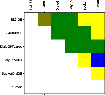
(a) Chatbot-DEB

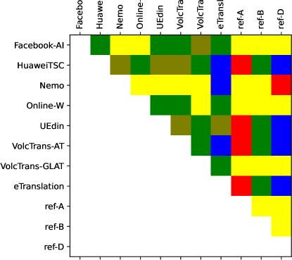
(b) WMT21-COMET

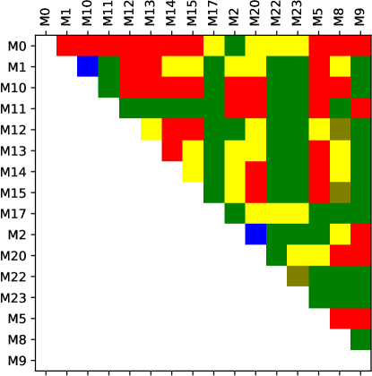
(c) SummEval Coh. Rouge

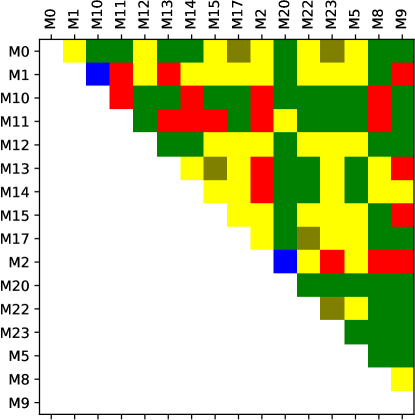
(d) SummEval Cons. BertScore

Figure 1: Comparison between the naive application of automated metrics and human evaluation. For each metric, the difference to the human evaluation is shown on the system-pair level. Green and Olive show agreement, Blue is an Omission Error, Yellow an Insertion Error, and Red denotes an Inversion Error.

Contributions. This paper has two main contributions: First, we propose a novel Bayesian statistical model of TG evaluation which integrates the various sources of uncertainty mentioned above. The model yields a more robust evaluation and has the flexibility to combine human and automated evaluations. The model can be used to determine whether two systems are significantly different or if they are of equal quality. The second contribution is an evaluation protocol that leverages the statistical model and reduces the amount of human ratings required.

We investigate the performance of the evaluation protocol in a case-study in three different TG tasks: chatbots, text summarization, and machine translation. Our case-study shows that using our contributions, we can almost completely correct for the errors emerging in the naive application of the metrics and that the amount of human ratings needed to produce robust evaluation outcomes is reduced by more than 50%.

2 Definition of Preference Metrics

In this section, we formally define preference metrics, their errors, and how to mitigate them. We then use this formalism to derive an effective evaluation protocol that can handle error-prone metrics. For the remainder of the paper, we define $\mathcal{I}$ as the set of all possible inputs (e.g., for machine translation all sentences in the source language), and $\mathcal{O}$ as the set of all possible outputs (e.g., all sentences in the target language). We start by defining a TG system as a function that takes an input and generates an output $\pi:\mathcal{I}\rightarrow\mathcal{O}$.

On an abstract level, we can define a preference metric as a function that takes as an input a triple consisting of: the input to a TG system (e.g., a sentence in the source language to be translated), the output of a system A, and the output of a system B (e.g., the translated sentences in the target language), and returns the preference rating. This is formalized as follows:

Definition 1 (Preference Metrics).

We call functions of the form $\mathcal{M}:\mathcal{I}\times\mathcal{O}\times\mathcal{O}\rightarrow\{>,=,<\}$ preference metrics. We call an outcome of $">"$ a win, $"="$ a draw, and $"<"$ a loss.

Note that the semantics of $\mathcal{M}(i,o_{1},o_{2})$ is to find out whether output $o_{1}$ is preferred over $o_{2}$. At this point, the notion of an output being preferred is to be taken abstractly, in a real-world application this would be realized by a concrete feature (better fluency, higher relevance, etc.).

Next, we introduce an oracle, which constitutes the ground-truth. When constructing an oracle in a real-world application, we would usually resort to human annotations.

Definition 2 (Preference Oracle).

The preference oracle is a function $\Omega:\mathcal{I}\times\mathcal{O}\times\mathcal{O}\rightarrow\{>,=,<\}$ such that

$$\Omega(i,o_{1},o_{2})=\begin{cases}>&\text{if $o_{1}$ is preferred to $o_{2}$}\\ =&\text{if there is no preference}\\ <&\text{if $o_{2}$ is preferred to $o_{1}$}\\ \end{cases}$$

Now we define the notion of an error-prone metric.

Definition 3 (Error-prone Metric).

A preference metric with independent confusion errors $\mathcal{M}$ is an error-prone metric where the probability of a given outcome is only dependent on the comparison oracle rating . Its confusion probabilities are defined as:

$$\mu_{c,c^{\prime}}=Pr(\mathcal{M}(i,o_{1},o_{2})=c|\Omega(i,o_{1},o_{2})=c^{\prime})$$ (1)

$$\forall c,c^{\prime}\in\{>,=,<\},\forall i\in\mathcal{I},\forall o_{1},o_{2}\in\mathcal{O}$$

The errors made by an error-prone preference metric can be represented by a confusion matrix with normalized columns, such that each entry in the matrix is a probability. The matrix $\bm{\mu}$ is called the mixture matrix of $\mathcal{M}$:

$$\bm{\mu}=\begin{pmatrix}\mu_{>>}&\mu_{>=}&\mu_{><}\\ \mu_{=>}&\mu_{==}&\mu_{=<}\\ \mu_{<>}&\mu_{<=}&\mu_{<<}\\ \end{pmatrix}$$ (2)

Note that the mixture matrix of an error-free metric is the identity matrix.

3 Statistical Model for Preference Metrics

1

2

3

Input : $\pi_{a},\pi_{b}$

Input : Set of metric judgments $M$

Input : Set of human judgments $A$

Output : Return preference rating

4

5begin

6      

7      $n_{cc^{\prime}}$ $\leftarrow$ CountConfusions ($A$, $M$, c, c’)

8      $n_{>},n_{=},n_{<}\leftarrow$ CountsFromAnn ($A$)

9      $m_{>},m_{=},m_{<}\leftarrow$ CountsFromAnn ($M$)

10      $\bm{\cdot\mu}_{>}\sim Dir(n_{>>}+1,n_{=>}+1,n_{<>}+1)$

11      $\bm{\cdot\mu}_{=}\sim Dir(n_{>=}+1,n_{==}+1,n_{<=}+1)$

12      $\bm{\cdot\mu}_{<}\sim Dir(n_{><}+1,n_{=<}+1,n_{<<}+1)$

13      $\bm{\mu}=(\bm{\mu_{\cdot>}},\bm{\mu_{\cdot=}},\bm{\mu_{\cdot<}})$

14      $\bm{p}\sim Dir(n_{>}+1,n_{=}+1,n_{<}+1)$

15      $m_{>},m_{=},m_{<}|\bm{p},\bm{\mu}\sim Tri(|M_{ij}|,\bm{\mu}\bm{p})$

16      $\left\{\tilde{\bm{p}}\right\}_{i=1}^{N}\leftarrow\textnormal{{{MCMCSamplePosterior}}}(\bm{p},N)$

17      $\theta=\frac{1}{N}\sum_{i=1}^{N}\mathbb{I}[\tilde{p_{i}}_{>}>\tilde{p_{i}}_{<}]$

18      if $\theta>1-\frac{\gamma}{2}$ then

19             return >

20       else if $\theta<\frac{\gamma}{2}$ then

21             return <

22       else

23             return =

24       end if

25      

26 end

27

Algorithm 1 Pairwise Decision Function.

In this section, we introduce the statistical model that is used to compare two TG systems $\pi_{a}$ and $\pi_{b}$. The model encompasses three main sources of uncertainty.

1. Uncertainty due to sample size of both error-free and error-prone ratings

2. Uncertainty introduced by errors from the error-prone metric

3. Uncertainty over the true error-rates of the error-prone metric

We build up the statistical model step-by-step by discussing each source of uncertainty. We apply the Bayesian approach which allows us to describe the process in terms of probability distributions that can be sampled by using Markov Chain Monte Carlo (MCMC) sampling (refer to Appendix A and B for additional details).

For the rest of the chapter, assume that we have access to a set of inputs $\{i_{1},\ldots,i_{n}\}\subseteq\mathcal{I}$, and the corresponding system outputs of $\pi_{a}$ and $\pi_{b}$, i.e., $o_{j}^{a}=\pi_{a}(i_{j})$, and $o_{j}^{b}=\pi_{b}(i_{j})$.

3.1 Step One: Direct Estimation of the Win-Rate Significance

For this, assume that we have access to the preference oracle $\Omega$ itself. Let $r_{j}^{\Omega}=\Omega(i_{j},o_{j}^{a},o_{j}^{b})$ be the output of the preference oracle. Let $\mathbb{I}^{x}[y]$ denote an index function that is equal to $\mathbb{I}^{x}[y]=1\iff x=y$, and $0$ otherwise. Then let $n_{>}=\sum_{j=1}^{n}\mathbb{I}^{>}[r_{j}^{\Omega}]$ denote the number of times $o_{j}^{a}$ was rated as being better than $o_{j}^{b}$. We analogously define $n_{<}=\sum_{j=1}^{n}\mathbb{I}^{<}[r_{j}^{\Omega}]$ the number of times $o_{j}^{a}$ was rated as being worse than $o_{j}^{b}$, and $n_{=}=\sum_{j=1}^{n}\mathbb{I}^{=}[r_{j}^{\Omega}]$ the number of draws. We use a Dirichlet distribution to model the posterior distribution for the given observations:

$$Pr(\bm{p}|N_{>}=n_{>},N_{=}=n_{=},N_{<}=n_{<})$$ (3)

$$\sim Dir(n_{>}+1,n_{=}+1,n_{<}+1)$$

where $\bm{p}=(p_{>},p_{=},p_{<})$ denotes the probability vector for the win-rate $p_{>}$, the draw-rate $p_{=}$, and the loss-rate $p_{<}$.

3.2 Step Two: Integrate the Metric-Errors

In this section, we assume a metric that makes mistakes, i.e., an error-prone metric $\mathcal{M}$. Let $r_{j}^{m}=\mathcal{M}(i_{j},o_{j}^{a},o_{j}^{b})$ denote the rating given by an error-prone metric for sample j. Analogous to before, we define $m_{>}=\sum_{j=1}^{n}\mathbb{I}^{>}[r_{j}^{m}]$ the number of times the error-prone metric prefers the output of system $\pi_{a}$ to that of $\pi_{b}$. The counts for equality and being worse are denoted by $m_{=}$ and $m_{<}$, respectively. Since $\mathcal{M}$ is an error-prone metric, the counts $m_{>,=,<}$ are not equal to the true counts $n_{>,=,<}$, which are yielded by an oracle. The errors made by the metric are characterized by its mixture matrix $\bm{\mu}$. In this section, we assume that the precise values of $\bm{\mu}$ are known. We note that the true probabilities $\bm{p}=(p_{>},p_{=},p_{<})$ are transformed by the mixture matrix to the error-prone ones by $\hat{\bm{p}}=(\hat{p}_{>},\hat{p}_{=},\hat{p}_{<})=\bm{\mu}\bm{p}$. We want to model the posterior distribution $p(\bm{p}|M_{>}=m_{>},M_{=}=m_{=},M_{<}=m_{<})$ of the true probabilities $\bm{p}$ given the observed error-prone ratings. This is done by combining the prior belief of $\bm{p}$ with the likelihood of the observed $m_{>,=,<}$ values, which can be modeled using a Multinomial distribution. We use a Dirichlet prior for $\bm{p}\sim Dirichlet(\alpha_{>},\alpha_{=},\alpha_{<})$. The parameters $\alpha_{c}$ are either chosen according to Equation 3, if we have access to oracle ratings, or set to $1$, which corresponds to a uniform prior.

$$\bm{p}\sim Dirichlet(\alpha_{>},\alpha_{=},\alpha_{<})$$

$$m_{>},m_{=},m_{<}|\bm{p}\sim Mult(n,\bm{\mu}\bm{p})$$

$$Pr(\bm{p}|m_{>},m_{=},m_{<})$$

$$\propto Pr(M_{>}=m_{>},M_{=}=m_{=},M_{<}=m_{<}|\bm{p})Pr(\bm{p})$$

3.3 Step Three: Integrate Uncertainty over Error Measurements

In a real-world scenario, the values of $\bm{\mu}$ must be estimated from data. This is achieved by comparing the error-prone metric outputs to a set of oracle outputs. For this, we use the following counts: $n_{c,c^{\prime}}=\sum_{i=1}^{n}\mathbb{I}^{c}[r_{j}^{m}]*\mathbb{I}^{c^{\prime}}[r_{j}^{\Omega}],\forall c,c^{\prime}\in\{>,=,<\}$. Thus, $n_{<,=}$ denotes the number of times the error-prone metric returns $<$ and the oracle returns $=$. In Bayesian terms, each column in the mixture matrix is modeled as a Dirichlet distribution.

$$\bm{\mu_{\cdot>}}=(\mu_{>>},\mu_{=>},\mu_{<>})^{\top}\sim Dirichlet(n_{.,>}+1)$$ (4)

$$\bm{\mu_{\cdot=}}=(\mu_{>=},\mu_{==},\mu_{<=})^{\top}\sim Dirichlet(n_{.,=}+1)$$

$$\bm{\mu_{\cdot<}}=(\mu_{><},\mu_{=<},\mu_{<<})^{\top}\sim Dirichlet(n_{.,<}+1)$$

$$\bm{\mu}=(\bm{\mu_{\cdot>}},\bm{\mu_{\cdot=}},\bm{\mu_{\cdot<}})$$

Thus, the mixture matrix is treated as a random variable. Putting all together, we define a joint posterior for $\bm{p}$ and $\bm{\mu}$ given the error-prone metric observation and the prior for $\bm{p}$ and $\bm{\mu}$.

$$\bm{p}\sim Dirichlet(\alpha_{>},\alpha_{=},\alpha_{<})$$

$$\bm{\mu}\sim\text{see Equation~{}\ref{eq:mu:diriclet}}$$

$$m_{>},m_{=},m_{<}|\bm{p},\bm{\mu}\sim Mult(n,\bm{\mu}\bm{p})$$

$$Pr(\bm{p},\bm{\mu}|m_{>},m_{=},m_{<})$$

$$\propto Pr(m_{>},m_{=},m_{<}|\bm{p},\bm{\mu})Pr(\bm{p})Pr(\bm{\mu})$$

3.4 Decision Function

Algorithm 1 shows how to apply the framework for one pair of systems $\pi_{a},\pi_{b}$ for a set of inputs $I$ and a set of human annotations $A$. First the metric $\mathcal{M}$ is used to generate the set of automated ratings $M$. Then the confusion counts $n_{c,c^{\prime}}$ are computed based on the human annotations and the metric ratings, which are used to create the distributions of the mixture matrix $\bm{\mu}$. Then the human annotations are used to estimate the prior distribution $Pr(\bm{p})$ of the comparison results. The metric samples are then used to estimate the posterior distribution $Pr(\bm{p},\bm{\mu}|m_{>},m_{=},m_{<})$. Each of the three steps presented above yields a posterior distribution for $\bm{p}=(p_{>},p_{=},p_{<})$. In order to decide whether system $\pi_{a}$ is better than system $\pi_{b}$, we need to check whether $p_{>}$ and $p_{<}$ are significantly different. For this, we draw a number of samples $\tilde{\bm{p}_{i}}$ from the posterior. This can in general be done using Markov Chain Monte Carlo sampling . We define a significance level $\gamma$ (e.g. $\gamma=0.05$) and consider the fraction of samples where $\tilde{p_{i}}_{>}>\tilde{p_{i}}_{<}$. If this fraction is greater than $1-\frac{\gamma}{2}$, then we regard the difference as being significant. Conversely, if the fraction is smaller than $\frac{\gamma}{2}$, then $\pi_{a}$ is significantly worse than $\pi_{b}$.

4 Evaluation Protocol

1

2

3

Input : $\Pi=\pi_{1},...\pi_{S}$

Input : An error-prone automated metric $\mathcal{M}$

Input : Budget for human annotations $B$

Input : Annotation batch size $N$

Input : Set of inputs $I$

Output : Partial Order of $\pi_{1},...\pi_{S}$

4

5begin

6      

7      UndecidedPairs $\leftarrow$ $\forall i,j:(\pi_{i},\pi_{j})\in\Pi\times\Pi$;

8      $A_{ij}$ $\leftarrow$ EmptySet ;

9       $M_{ij}=\{\mathcal{M}(i_{k},\pi_{i}(i_{k}),\pi_{j}(i_{k}))|\forall k\in|I|\}$

10      while $B>0$ and $|\textnormal{{{UndecidedPairs}}}|>0$ do

11             foreach $\pi_{i},\pi_{j}\in$ UndecidedPairs do

12                   $A_{ij}\leftarrow A_{ij}\cup$ CollAnn ($N$, $\pi_{i}$, $\pi_{j}$) $B\leftarrow B-N$

13             end foreach

14            foreach $\pi_{i},\pi_{j}\in$ UndecidedPairs do

15                   op = DecisionFunction ($A_{ij}$, $M_{ij}$, $\pi_{i}$, $\pi_{j}$)

16                  if op $\in\{<,>\}$ then

17                         UndecidedPairs $\leftarrow$ UndecidedPairs $\setminus(\pi_{i},\pi_{j})$

18                   end if

19                  

20             end foreach

21            

22       end while

23      return ComputePartialOrder ($\Pi\times\Pi\setminus$ UndecidedPairs);

24 end

25

Algorithm 2 Evaluation Protocol

In this section, we present an evaluation protocol combining human and automated metric ratings assuming a limited budget for human annotations. More formally, given a set of TG systems $\pi_{1},...,\pi_{S}$, we want to create a partial order, where $\pi_{i}>\pi_{j}$ if the win-rate of $\pi_{i}$ is significantly greater than the one from $\pi_{j}$. The evaluation protocol is depicted in Algorithm 2. The protocol leverages the statistical framework to reduce the amount of human annotations needed by leveraging the metric judgments. This works as follows: We are given a set of inputs $I$ (which corresponds to a test set), a set of TG systems $\{\pi_{1},...,\pi_{S}\}$ to be ranked, an automated metric $\mathcal{M}$, and an annotation budget $B$, which is the maximum allowed amount of annotations. The result of the protocol is a (potentially) partial order of the TG systems.

The protocol starts with a set of undecided system pairs, which initially consists of all pairs of systems, and an empty set of human annotations for each pair of systems $A_{ij}$. In a first step, the metric $\mathcal{M}$ computes the scores $M_{ij}$ for each pair of systems. That is, for all inputs in $I$ all TG systems generate their outputs, which are then evaluated using $\mathcal{M}$.

Then we repeat the following process until our budget is empty. First we extend $A_{ij}$ with a batch of $N$ human annotations for each pair of undecided systems. We then iterate over the undecided system pairs and use the decision function from Algorithm 1 (see Section 3) to decide whether two given systems are significantly different given the current set of annotations and metric ratings. If so, the pair is removed from the set of undecided pairs. When the budget is empty or all system pairs are decided, a (potentially) partial order is computed. The decision function leverages human and automated ratings to state whether one system is significantly better than the other.

The advantage the protocol is two-fold. First, it exploits the fact that some system pairs are easier to distinguish than others. In cases where $|p_{>}-p_{<}|$ is large we need fewer human annotations to achieve the significance threshold. Compared to the setting where we allocate the same number of human annotations for each pair of systems, this allows us to spend more of the annotation budget on difficult system pairs. This approach can be used even in the absence of automated ratings. Second, our framework allows for a seamless combination of ratings from both humans and an automated metric.

5 Case Studies - Setup

In this section, we present three case studies where we apply the evaluation protocol outlined in Algorithm 2. As showcases, we use three domains: the WMT 21 metrics task data Freitag et al. (2021) for machine translation, the SummEval data Fabbri et al. (2021) for summarization, and data collected for conversational dialogue systems (see Appendix C). Table 1 gives an overview of the setting. For each domain, we investigate a set of metrics applied to outputs of a set of TG systems. We provide the details of the TG systems and the metrics in Appendix C.

	Chatbot	SummEval	WMT21
Data	BST	CNN/DM	News EN->DE
Metrics	5	7	4
TG Systems	6	11	16
Human Ratings	50	100	500
Metric Ratings	1k	11k	1k

Table 1: Overview of the data used. The ratings refer to the number of ratings available for each pair of TG systems.

Chatbot: For the chatbot domain, we used the ParlAI framework Miller et al. (2017) to generate 1000 outputs for 5 different TG systems on the BlendedSkillTask (BST) dataset Smith et al. (2020). We then used the DialEval framework by Yeh et al. (2021) to run the outputs on 5 different metrics: DEB Sai et al. (2020), GRADE Huang et al. (2020), HolisticEval Pang et al. (2020), MAUDE Sinha et al. (2020), and USL-H Phy et al. (2020). In addition, we used Amazon Mechanical Turk to annotate 50 pairwise outputs.
SummEval: For the summarization domain, we used the SummEval framework Fabbri et al. (2021), which provides the outputs of 16 different summarization tools on the CNN/DailyMail corpus Nallapati et al. (2016), as well as 100 expert annotations for each of these systems for each of the features: relevance, coherence, consistency, and fluency. We used the SummEval framework to generate 11k pairwise ratings by 7 different automated metrics: BertScore Zhang et al. (2019), BLANC Vasilyev et al. (2020), CIDEr Vedantam et al. (2015), Rouge-L Lin (2004), S3 Peyrard et al. (2017), SummaQA Scialom et al. (2019), and SUPERT Gao et al. (2020).
WMT21: For machine translation, we used the WMT21 metrics task data Freitag et al. (2021). In this work, we only focus on the English to German language pair and the news domain, where eight machine translation systems were evaluated, plus three human references for each input which were also regarded as TG systems (resulting in eleven TG systems). Although the WMT21 metrics task inspected 15 different automated metrics, we only focused on four of them (we selected the most prominent ones): BleuRT Sellam et al. (2020), COMET Rei et al. (2020), C-SPEC Takahashi et al. (2021), and sentence-level BLEU Papineni et al. (2002). For each TG system there are 500 expert MQM annotations, and for each metric there are 1000 metric ratings.

6 Case Studies - Results

In this section, we discuss the results of the case study. We use the error-measures that we presented in List 1 in the introduction. Furthermore, for each system pair we compute the Kullback-Leibler Divergence (KLD) between the mode of the posterior in Equation 3 based on all human annotations $\bm{p}_{hum}$ and the mean estimated by running Algorithm 2 $\bm{p}_{prot}$. We then report the average over all pairs of systems: $\frac{2}{S(S-1)}\sum_{j>i}KLD(\bm{p_{prot}}^{(i,j)}||\bm{p_{hum}}^{(i,j)})$. Note that in Tables 2 and 3, we only report the Relevance part of the SummEval data due to space limitations. The results for the other features are in Appendix D.

Domain	Corr.	Inv.	Omi..	Ins.	KLD
Chatbot	0.47	0.1	0.10	0.33	0.46
Summeval Rel.	0.55	0.19	0.03	0.23	0.28
WMT21	0.52	0.07	0.10	0.31	0.52

Table 2: Average frequency of Error Types for all metrics if metrics are applied naively. Correct (Cor.), Inverted (Inv.), Omission (Omi.), and Insertion (Ins.).

The naive application of metrics yields many errors. When applying the metrics naively, i.e. by simply checking whether $m_{>}$ is significantly bigger than $m_{<}$, then this introduces many cases where systems that are not significantly different are rated as such. In Table 2 the average error rates for each error type are shown (the full result table is found in Appendix D). Overall the Insertion error type dominates (averaging at 23% to 33%). That is, in all domains, the metrics have a strong tendency to suggest differences between systems that are not statistically significant according to the human evaluation. The rate of inversion errors depends on the domain and metrics used. For the chatbot domain, the average Inversion error rate lies at 10%. For SummEval-Relevance the Inversion error rates lie at an average of 23%. The average KLD scores are high, which indicates that the naive application of metrics yields distributions that are in high disagreement with the human evaluation.

Metric	Corr.	Inv.	Omi.	Ins.	KLD	Ann.
Chatbot Domain
Human	0.93	0.00	0.00	0.07	0.05	0.59
DEB	0.93	0.00	0.00	0.07	0.06	0.49
GRADE	0.87	0.00	0.00	0.13	0.05	0.53
HOLISTIC	0.87	0.00	0.00	0.13	0.05	0.52
MAUDE	0.87	0.00	0.00	0.13	0.05	0.53
USL-H	0.87	0.00	0.00	0.13	0.05	0.52
Summeval Relevance Domain
Human	0.96	0.00	0.00	0.04	0.07	0.43
BertScore	0.90	0.00	0.01	0.09	0.06	0.40
BLANC	0.93	0.00	0.02	0.06	0.05	0.41
CIDEr	0.93	0.00	0.01	0.06	0.06	0.42
ROUGE-L	0.92	0.00	0.01	0.08	0.05	0.41
S3	0.93	0.00	0.01	0.07	0.06	0.41
SummaQA	0.92	0.00	0.01	0.08	0.05	0.41
SUPERT	0.91	0.00	0.01	0.08	0.06	0.39
WMT21 Domain
Human	0.65	0.00	0.00	0.35	0.06	0.34
BleuRT	0.65	0.00	0.00	0.35	0.06	0.34
C-SPEC	0.65	0.00	0.00	0.35	0.06	0.33
COMET	0.65	0.00	0.00	0.35	0.06	0.34
BLEU	0.65	0.00	0.00	0.35	0.05	0.34

Table 3: Frequency of Error Types for all metrics if the protocol is applied. Correct (Cor.), Inverted (Inv.), Omission (Omi.), Insertion (Ins.), and the fraction of annotations needed with the protocol (Ann.).

The evaluation protocol is able to recreate the original results. Table 3 shows the results of applying the protocol described in Algorithm 2. We also report the results achieved when applying the protocol using only human ratings (i.e., leaving $M_{ij}$ empty), as well as the result of an ideal metric in the SummEval - Relevance case. First, we note that there are no Inversion Errors, almost no Omission Errors, and there is a high Correctness score. For the Chatbot and SummEval domain the outcomes agree in around 90% to those of the human evaluation. For the WTM21 domain, the agreement is lower at 65%. The most common error type is the Insertion Error. In our setting this can be explained by the fact that we are using the outcomes of significance tests to compare the human to the protocol evaluation. Thus, using corrected metric samples increases the amount of samples, which leads to pairs being rated as significantly different. Since the ratings are based on our decision function, which takes into account different sources of uncertainty, the Insertions are not necessarily wrong. In fact one reason to use automated evaluation is to find differences between system that would be too expensive to discover with human annotations.

A different view for comparing the outcomes of the evaluations is given by the KLD score, which reports how close the distribution $\bm{p}_{prot}$ is to the original human evaluation. This view removes the significance test from the equation, and better showcases the disagreement between the protocol and the original human evaluation. In all cases the KLD scores are very low, which shows that the protocol yields results comparable to the original human evaluation.

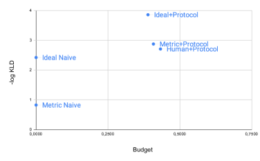
Figure 2: Budget vs. Kullback-Leibler Divergence

In terms of the number of annotations needed, there are two measures. First, we compare the number of annotations needed by the protocol to the one needed by the full human evaluation. Here, the application of our protocol reduces the amount of humans annotation by more than half in most cases. For the WMT21 we can even reduce it by two thirds. The second view is comparing the number of annotations needed by the protocol to the annotations needed when the protocol is applied to human ratings only. For the Chatbot and SummEval domain, leveraging automated metrics results in less data needed (up to 10% for the Chatbot domain, and 5% for the SummEval domain). For the WMT21 domain, only 1% difference is measured. We assume that this are due to the fact that the metrics are not yet of high enough quality to yield the boost needed to have a large impact.
Summary. Figure 2 summarizes the main outcomes of this work. The Figure shows the number of annotations (x-axis) in relation to the negative log-KLD score achieved (y-axis). The full human evaluation is set as reference, that is, using 100% of annotations, and a KLD score of 0 (thus, not shown). The Figure shows that on average using the full protocol on real-world metrics yields using 40% of annotations, and achieving a KLD score of 0.08. On the other hand, not using metric ratings in the protocol needs 43% of annotations and achieving a worse KLD score of 0.6. The naive application of the metrics does not need any annotations but yields high KLD scores (1.6 on average). To showcase an upper limit, we also added the KLD divergence for an ideal metric, which we simulated using the Bayesian model, where we use a fixed $\bm{\mu}$ (see Appendix E for details). The ideal metric only needs 38% of annotation, and achieves a KLD score of 0.02. An ideal metric would also achieve a low KLD when applied naively.

7 Related Work

We here focus on approaches that discuss theory-driven analysis of metrics-based evaluation of TG systems that involve human annotations.

Chaganty et al. (2018) propose an approach to combine human and metrics-based evaluation using control variates to reduce biases in automated metrics and save annotation costs. They explore automated scalar metrics in the Summarization and QA domain and find that their approach can lead to marginal reductions of the required human annotations. They conclude that further improvement of automated metrics and exploration of ranking-based evaluation are potential future directions. One interesting take-away from this work is the influence of the quality of the human annotations. Currently, we approximate the oracle preference ratings through human annotations without explicitly modeling uncertainty stemming from annotator disagreement. Wei and Jia (2021) pick up this point and apply a statistical approach to identify a setting in which automated metrics for Machine Translation and Summarization are more precise than human annotations: When the qualitative difference is small and there are only few human annotations. They argue that the reason is that while human annotations are unbiased, they have a high variance. Conversely, automatic metrics tend to have a high bias but low variance. Furthermore, they apply the bias-variance-noise decomposition from Domingos (2000) to analyse sources of errors in evaluation and asses bias levels in automated metrics. Our analysis, in comparison, is more fine-grained in terms of categorizing metric errors, and we propose how to combine human and metric evaluation under a budget constraint. Similar to this work, von Däniken et al. (2022) propose a model that captures uncertainties stemming from imperfect metrics and insufficiently sized test sets. With their framework, the required size of a test set that is needed to distinguish a given difference in performance between two systems with a given automated metric can be calculated. Their investigation is limited to the case when scalar metrics are converted to binary metrics, however. Card et al. (2020) also analyse the required data set sizes that enable the detection of significant differences between systems, but they do not account for metric errors explicitly. Hashimoto et al. (2019) propose an evaluation approach that combines human and automated evaluation in a statistical framework to estimate diversity and quality of NLG systems jointly. Their focus is the creation of a novel metric, while our goal is to evaluate existing ones and to combine them with human annotations to obtain robust evaluations.

8 Conclusion

In this work, we introduced a novel Bayesian model that explicitly handles errors from automated metrics at the sample level. We then proposed an evaluation protocol that leverages this statistical model to reduce the amount of human annotations needed while yielding similar evaluation outcomes. We applied the protocol to three tasks in a case study. Namely, Dialogue Systems, Summarization, and Machine Translation. The results show that the Bayesian model is able to successfully include various types of uncertainty, which leads to more trustworthy applications of automated metrics. When applying the protocol, we achieve similar results as a purely human evaluation with only half the annotations needed.

Limitations

Human Ratings as Oracle.

In this work, we make the strong assumption that human ratings are equivalent to the oracle. As noted in the introduction, human evaluation is hard to setup and does not always lead to satisfactory agreement scores. However, for SummEval and WMT21 the human ratings are provided by experts, and thus, can be seen as close to oracle ratings. For the Dialogue domain, the ratings are made by crowdsourcing where we applied MACE Hovy et al. (2013) to get the highest quality ratings. In future work, we will integrate the uncertainty of the human evaluation in the Bayesian model as well, which is not trivial.

Pairwise $\bm{\mu}$.

We noted that the for each pair of systems, the mixture matrix is different. As a consequence, the errors made by the metric must be computed for each pair of systems separately, which is more cost-intensive. In future work, we aim to develop methods to transfer the knowledge from one system pair to another. This also highlights one issue of automated metrics, namely, that they are biased towards certain output types, which are exhibited by certain TG systems.

Draws are ignored.

One issue with preference-based ratings is the question of how to handle draws on the sample basis. Currently, we use $p_{>}$ and $p_{<}$ to decide if two systems are significantly different. However, if we consider the case of $p_{>}=0.02$, $p_{<}=0.01$, and $p_{=}=0.97$, then with enough samples, we will measure a statistical significant difference between the two systems. However, in 97% of cases the outputs are of equal quality. Thus, can we really state that one system is better than the other?

Statistical Significance Decision.

To compare the outcomes of the automated evaluation to the human evaluation, we rely on statistical significance testing. For this, we use the standard approaches, which are widely adopted. However, we noted that the significance decisions are rather arbitrary and make it hard to compare two evaluations, especially the interpretation of Insertion Errors is not trivial. The large amounts of additional automated metric ratings result in some pairs being rated as significantly different. However, it is not clear whether this is a mistake or if we were able to distinguish two systems that were not distinguishable due to too little data. The KLD score gives better insights for this as it compares distributions.

Differences in Samples.

Currently, we disregard the fact that there are samples which are harder to rate than others. In fact, we treat each sample as being equal in Defintion 3. However, the sample difficulty could be leveraged to distinguish different systems from each other. For instance, if two machine translation systems are evaluated only on easy samples, then they might be rated as being of equal quality. However, a test on a harder sample might show the difference in capabilities between the two systems.

Conversion to Preference Ratings.

Current automated metrics are built such that they return a scalar value $\in\mathbf{R}$ to rate a given pair of input and output. We have to transform these values into preference ratings by looking at the sign of the difference between the ratings of two outputs (see Appendix C). This leads to a few problems. First, there are only few draws, since metrics rarely return the exact same floating point value for two different outputs. Second, we disregard the magnitude of the scalar value. The magnitude can be used to assess the certainty of the preference of one output against another. In preliminary experiments we tried including a minimal threshold that the difference needs to surpass in order to be regarded as a preference decision. This will have to be explored in more detail in future work.

Current Metric performance.

Since the current metrics are not yet of high enough quality, the impact they have on the protocol is small. This might give the impression that the protocol does not offer any remedy. However, the results show that our Bayesian model is able to rectify the overconfidence of low-performance metrics, and in cases where a metric is of low quality, its impact is reduced.

Appendix A Derivations

Dirichlet.

We will first explain the usage of Dirichlet distributions in Equations 3 and 4. The Dirichlet distribution of order $K$ is defined for all $K$ dimensional probability vectors $\bm{p}=(p_{1},\dots,p_{K})$ such that $\sum_{i=1}^{K}p_{i}=1$ and $p_{i}\geq 0$. It has $K$ parameters $\bm{\alpha}=(\alpha_{1},\dots,\alpha_{K})$ and its density is:

$$p(\bm{p}|\bm{\alpha})=\frac{1}{B(\bm{\alpha})}\prod_{i=1}^{K}p_{i}^{\alpha_{i}-1}$$

, where $B(\bm{\alpha})$ is the multivariate Beta function used to normalize the distribution. Note that if all $\alpha_{i}=1$ then the distribution is constant at all points $\bm{p}$, meaning it is equivalent to the uniform distribution in that case. Our main interest in using the Dirichlet distribution is because it is the conjugate prior of the Multinomial distribution. In Section 3 the counts from the oracle ratings $n_{>}$, $n_{=}$, and $n_{<}$ follow a Multinomial distribution with unknown probabilities $\bm{p}=(p_{>},p_{=},p_{<})$, meaning that:

$$P(N_{+}=n_{+},N_{=}=n_{=},N_{<}=n_{<}|\bm{p})$$

$$=\frac{(n_{>}+n_{=}+n_{<})}{n_{>}!n_{=}!n_{<}!}p_{>}^{n_{>}}p_{=}^{n_{=}}p_{<}^{n_{<}}$$

If we assume a Dirichlet prior for $\bm{p}\sim Dirichlet(\alpha_{>},\alpha_{=},\alpha_{<})$ then we can compute its posterior:

$$p(\bm{p}|N)\propto P(N|\bm{p})p(\bm{p})$$

$$\propto p_{>}^{n_{>}}p_{=}^{n_{=}}p_{<}^{n_{<}}p_{>}^{\alpha_{>}-1}p_{=}^{\alpha_{=}-1}p_{<}^{\alpha_{<}-1}$$

$$\propto p_{>}^{\alpha_{<}+n_{<}-1}p_{=}^{\alpha_{=}+n_{=}-1}p_{<}^{\alpha_{<}+n_{<}-1}$$

We left out the normalization constants in this derivation. We can see that on the final line we arrive at the density of an updated Dirichlet distribution $Dirichlet(\alpha_{>}+n_{>},\alpha_{=}+n_{=},\alpha_{<}+n_{<})$. Setting $\alpha_{i}=1$ we get our result in Equation 3.

We can apply the same principle to the columns of $\bm{\mu}$. The first column $\bm{\mu}_{\cdot>}=(\mu_{>>},\mu_{=>},\mu_{<>})^{T}$ denotes the conditional probabilities of getting a specific outcome from the metric conditioned on the oracle rating being $>$. The associated confusion counts $n_{>>}$, $n_{=>}$, and $n_{<>}$ again follow a Trinomial distribution with outcome probabilities of $\bm{\mu}_{\cdot>}$. If we again assume a uniform prior for $\bm{\mu}_{\cdot>}$ then we can derive the posteriors in Equation 4.

Mixture.

In Sections 3.2 and 3.3 we use the fact that the probabilities associated with the counts of metric ratings is $\hat{\bm{p}}=\bm{\mu}\bm{p}$. We know that $\hat{p}_{>}=P(\mathcal{M}(i_{j},o_{j}^{a},o_{j}^{b})=\text{>})$. Using the law of total probability:

$$\hat{p}_{>}=\sum_{c\in\{>,=,<\}} P(\mathcal{M}(i_{j},o_{j}^{a},o_{j}^{b})=\text{>}|\Omega(i_{j},o_{j}^{a},o_{j}^{b})=c)$$

$$P(\Omega(i_{j},o_{j}^{a},o_{j}^{b})=c)$$

We note that $P(\Omega(i_{j},o_{j}^{a},o_{j}^{b})=c)=p_{c}$, and therefore $\hat{p}_{>}=\sum_{c\in\{>,=,<\}}\mu_{>c}p_{c}$ and analogously for $\hat{p}_{=}$ and $\hat{p}_{<}$. This leads us to our original statement $\hat{\bm{p}}=\bm{\mu}\bm{p}$.

Using Annotations multiple times.

In Algorithm 1 it can be unclear which subsets of annotations should be used for the various counts. In general, the test set of inputs $\mathcal{I}$ can be split into three subsets: $\mathcal{I}_{M,A}$, the samples for which we have paired ratings from both the metric and humans, $\mathcal{I}_{M}$, the samples for which we have only ratings from the automated metric, and $\mathcal{I}_{A}$, the samples for which we only have human ratings. It is relatively obvious that we can use $\mathcal{I}_{M}$ to count $m_{>},m_{=},m_{<}$, $\mathcal{I}_{A}$ for $n_{>},n_{=},n_{<}$, and $\mathcal{I}_{M,A}$ for the confusion counts $n_{cc^{\prime}}$. The question is whether it is sound to use the ratings from $\mathcal{I}_{M,A}$ to augment $n_{c}$ and $m_{c}$. In general, it should not be an issue to use the human ratings in $\mathcal{I}_{M,A}$ as additional counts for $n_{>},n_{=},n_{<}$. But we must not use the metric ratings to get additional counts $m_{>},m_{=},m_{<}$. This means that, in principal, $\mathcal{I}_{A}$ could be empty.

Appendix B Markov Chain Monte Carlo (MCMC) Sampling

Markov Chain Monte Carlo (MCMC) methods are often used in Bayesian modelling when there is no analytic closed form solution for the resulting posterior. The main idea is that expected values of functions of the posterior can be reasonably approximated by averaging over samples drawn from it (Metropolis and Ulam, 1949). Samples are generated sequentially, and the next sample is usually generated by first modifying the current sample randomly and then either accepting or rejecting it based on its likelihood. We refer the interested reader to Andrieu et al. (2003) for an introduction.

We use the Numpyro (Bingham et al., 2019; Phan et al., 2019) library to implement the framework laid out in Section 3. We use the built-in No-U-Turn (NUTS) Sampler (Hoffman and Gelman, 2014). When running the decision function laid out in Algorithm 1, we run 5 chains in parallel. We use a warm-up period of 2000 samples per chain, which are discarded, and draw 10000 samples per chain to keep and compute the difference in win rates.

Appendix C Case Study Details

For the case studies, we require two types of ratings: preference ratings made by humans to simulate the oracle $\Omega$, and metric ratings for the error-prone ratings $\mathcal{M}$. We collect this data for three types of domains: Conversational Dialogue Systems, Automated Text Summarization, and Machine Translation.

Since most metrics return a scalar value, we need to transform them into a preference rating, which is done as follows:

Definition 4 (Scalar Metric).

We call real valued functions of inputs and outputs scalar metrics: $\mathcal{M}_{s}:\mathcal{I}\times\mathcal{O}\rightarrow\mathbb{R}$.

A preference metric can be constructed from a scalar metric as follows:

Definition 5.

The derived comparison metric $\mathcal{M}$ of a given scalar metric $\mathcal{M}_{s}$ is defined as

$$\mathcal{M}(i,o_{1},o_{2})=\begin{cases}>&\mathcal{M}_{s}(i,o_{1})>\mathcal{M}_{s}(i,o_{2})\\ =&\textit{otherwise}\\ <&\mathcal{M}_{s}(i,o_{1})<\mathcal{M}_{s}(i,o_{2})\\ \end{cases}$$

C.1 Dialog System Data Collection

For the Dialog domain, we used the ParlAI framework Miller et al. (2017) to generate the outputs of systems. For this, we selected 5 state-of-the-art dialog systems, and used ParlAI to generate response for a static context. The Dialogue Systems are:

• Blenderbot 1.0 - 400distill (BL400distill). BlenderBot 1.0 Shuster et al. (2022b) is a transformer-based encoder-decoder bot trained on the Blended Skill Task (BST) data Smith et al. (2020).

• Blenderbot 2.0 - 3B Params (BL2-3B). The BlenderBot 2.0 extends Blenderbot 1.0 with internet access Komeili et al. (2022) and a long-term memory Xu et al. (2022).

• DialoGPT. DialoGPT Zhang et al. (2020) is a decoder-only dialogue system that fine-tunes GPT-2 Radford et al. on the Reddit dataset proposed by the DialoGPT authors.

• PolyEncoder. The PolyEnocder Humeau et al. (2020) is a retrieval based dialogue system, which selects the most suitable response from a set of candidates.

• SeekerDial3B. SeekerDial Shuster et al. (2022a) improves on the internet search proposed in BlenderBot 2.0

We used ParlAI to generate the response of each of the dialogue systems for 1000 static contexts from the Blended Skill Task (BST) test set. From this set, we selected 50 contexts, and generated all pairwise outputs between all 5 dialogue systems and the human reference. That is, for each context, there are 15 pairs of outputs to be rated.

We let workers on Amazon Mechanical Turk  perform a preference rating. That is, for each pair of output, the workers decided, which output is more appropriate. Figure 3 shows the annotation tool. Each sample was annotated by three workers. Each worker is payed 15 cents per annotation, and at a rate of 1.5 annotations per minute on average, they achieve a wage of 12$ per hour. We used workers with the Master status and restricted their geographic location to English-speaking countries (USA, UK, Canada, Ireland, and Australia). In Figure 4 shows the instructions given to the annotators. The annotations are ratings on the overall adequacy of the utterances. Since each sample is annotated by three different workers, we aggregate the ratings using the MACE Hovy et al. (2013) software, which computes a trustworthiness score for each annotator and generates a weighted average to get the final label. Note that this annotation scheme directly yields preference ratings according to our framework.

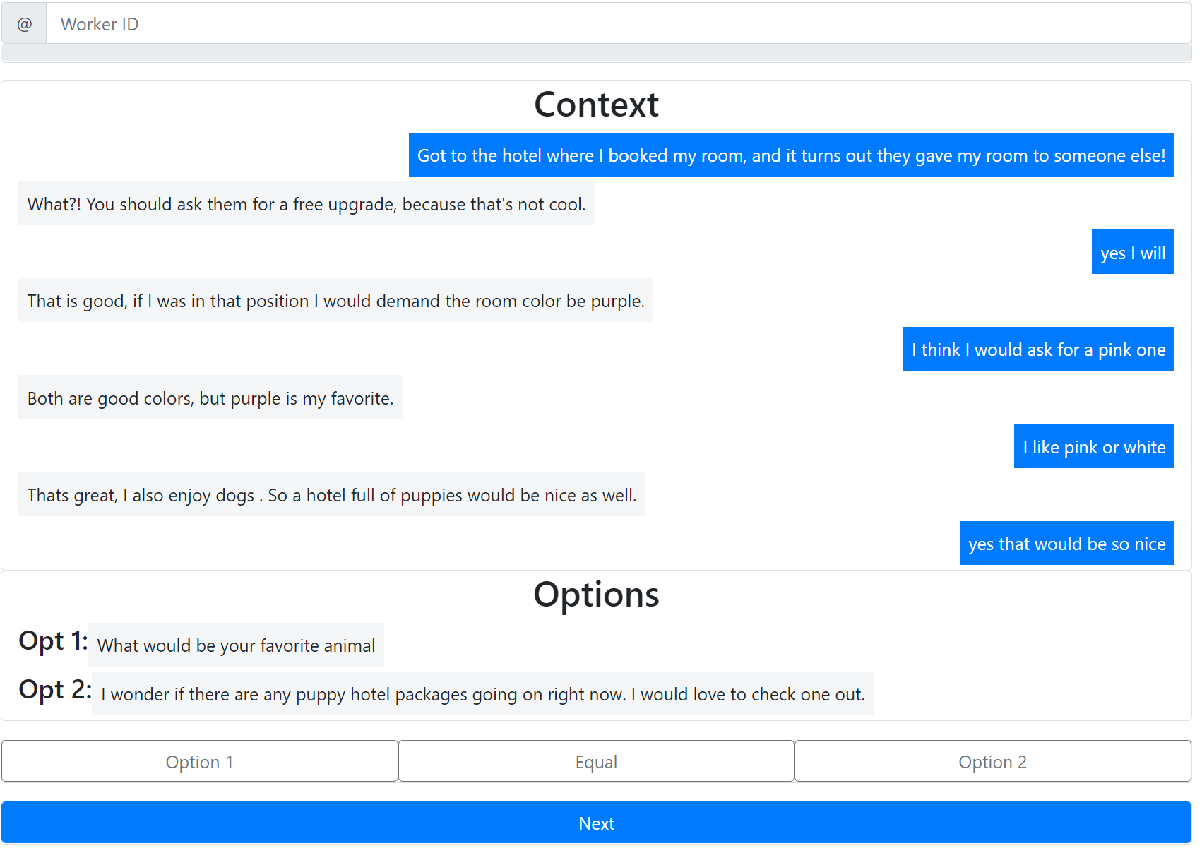
Figure 3: Screenshot of the Dialogue Annotation Tool.

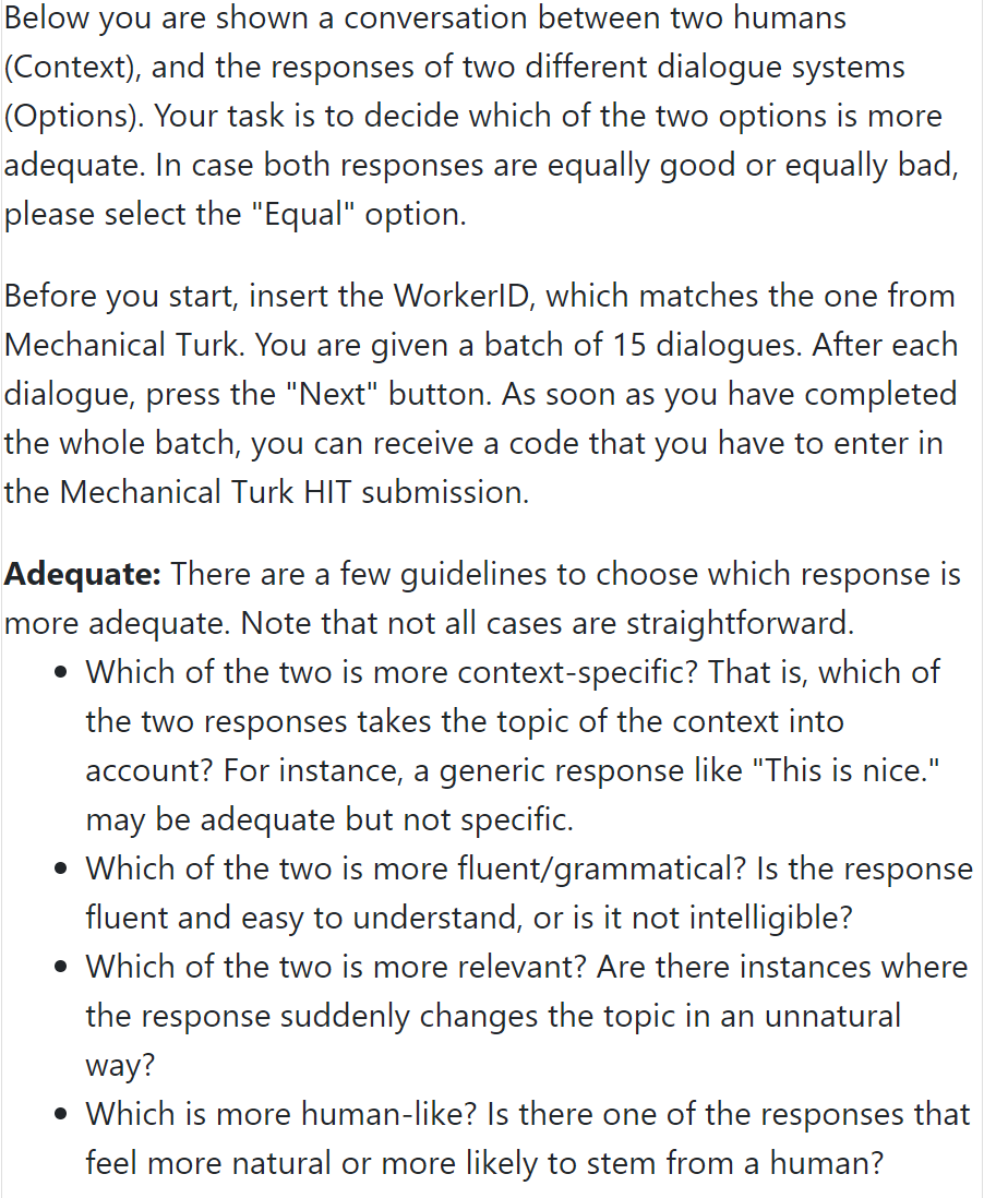
Figure 4: Screenshot of the Instruction of the Dialogue Annotation Tool.

In order to generate the metric ratings, we used the DialEval framework by Yeh et al. (2021), which integrates a large pool of metrics. We selected five metrics that were easy to setup and achieved decent correlations to human judgments in the evaluation by Yeh et al. (2021). Since the metrics return scalar values for each sample, we create preference ratings as suggested in Definition 5. Since the scalar metrics yield real numbered values, there are almost no cases where the derived preference rating yields a draw.

C.2 Summarization Data Collection

For the Summarization domain, we use the data provided by the SummEval framework Fabbri et al. (2021). It contains data from the Dailymail/CNN dataset Nallapati et al. (2016), which contains a test set of 11k samples. The SummEval framework contains the outputs of 23 summarization systems (for a detailed description of these systems, we refer the reader to Section 3.2 of Fabbri et al. (2021)). For 16 of the 23 summarization systems, the authors let 100 generated outputs be rated by three experts on the four characteristics: fluency, consistency, coherence, and relevance. Since these ratings are on a Likert-scale, we transformed those ratings into preference ratings by averaging the three ratings per sample, and applying the transformation proposed in definition 5.

We chose 7 automated metrics based on their popularity and ease of setup. We applied the SummEval framework to generate the automated ratings for each of the 16 summarization systems on the full test set. Analogous to above, we converted the scalar ratings to pairwise ratings by applying definition 5.

C.3 Machine Translation Data Collection

For the Machine Translation domain, we used the WMT-21 Freitag et al. (2021) metrics task data. For space limitations, we used the EN$\rightarrow$DE section of the data only. The WMT-21 dataset consists of 15 different metrics for 8 machine translation systems and 3 human references. The human annotations consist of 500 MQM ratings Lommel et al. (2014) done by expert translators. To create preference ratings, we computed the average score of a sample, and compared the score of two outputs of two different systems for the same input by applying definition 5.

The WMT-21 dataset already contains the ratings of the automated metrics for 1000 samples, out of which 500 overlap with the samples annotated by humans. Thus, we generated pairwise ratings by applying definition 5.

Appendix D Full Results

Tables 4 and 5 show the results for all the metrics over all tasks and features. Figure 5 shows the pairwise errors when applying our protocol.

Metric	Corr.	Inv.	Omi.	Ins.	KLD
Chatbot Domain
deb	0.60	0.00	0.07	0.33	0.39
grade	0.53	0.07	0.20	0.20	0.53
holistic	0.27	0.20	0.13	0.40	0.57
maude	0.40	0.13	0.13	0.34	0.42
usl	0.53	0.07	0.00	0.40	0.40
Summeval Coherence Domain
BertScore	0.58	0.22	0.00	0.20	0.35
BLANC	0.45	0.29	0.02	0.24	0.33
CIDEr	0.38	0.36	0.02	0.24	0.43
ROUGE-L	0.45	0.33	0.00	0.22	0.34
S3	0.53	0.24	0.01	0.22	0.35
SummaQA	0.53	0.19	0.07	0.21	0.31
SUPERT	0.45	0.25	0.06	0.24	0.38
Summeval Consistency Domain
BertScore	0.49	0.16	0.00	0.35	1.92
BLANC	0.44	0.15	0.02	0.39	1.74
CIDEr	0.30	0.30	0.02	0.38	2.17
ROUGE-L	0.35	0.25	0.02	0.38	1.98
S3	0.46	0.17	0.01	0.37	1.90
SummaQA	0.55	0.09	0.03	0.33	1.81
SUPERT	0.46	0.13	0.04	0.38	1.76
Summeval Fluency Domain
BertScore	0.46	0.14	0.00	0.40	1.03
BLANC	0.40	0.16	0.01	0.43	0.98
CIDEr	0.34	0.21	0.02	0.43	1.08
ROUGE-L	0.41	0.18	0.00	0.42	0.99
S3	0.42	0.16	0.01	0.42	1.03
SummaQA	0.48	0.08	0.05	0.39	0.97
SUPERT	0.43	0.12	0.03	0.42	1.06
Summeval Relevance Domain
BertScore	0.64	0.13	0.01	0.22	0.26
BLANC	0.51	0.23	0.02	0.25	0.25
CIDEr	0.43	0.29	0.03	0.25	0.35
ROUGE-L	0.52	0.24	0.01	0.23	0.25
S3	0.62	0.15	0.01	0.23	0.26
SummaQA	0.61	0.11	0.07	0.22	0.23
SUPERT	0.51	0.20	0.05	0.24	0.35
Ideal-$\mathcal{M}$	0.75	0.00	0.00	0.25	0.02
WMT21 Domain
BleuRT	0.47	0.02	0.13	0.38	0.46
C-SPEC	0.78	0.00	0.07	0.15	0.53
COMET	0.40	0.09	0.13	0.38	0.65
BLEU	0.44	0.16	0.07	0.33	0.43

Table 4: Frequency of Error Types for all metrics if metrics are applied naively. Correct (Cor.), Inverted (Inv.), Omission (Omi.), Insertion (Ins.), and the fraction of annotations needed with the protocol (Ann.).

Metric	Corr.	Inv.	Omi.	Ins.	KLD	Ann.
Chatbot Domain
Human	0.93	0.00	0.00	0.07	0.05	0.59
DEB	0.93	0.00	0.00	0.07	0.06	0.49
GRADE	0.87	0.00	0.00	0.13	0.05	0.53
HOLISTIC	0.87	0.00	0.00	0.13	0.05	0.52
MAUDE	0.87	0.00	0.00	0.13	0.05	0.53
USL-H	0.87	0.00	0.00	0.13	0.05	0.52
Summeval Coherence Domain
Human	0.97	0.00	0.00	0.03	0.04	0.42
BertScore	0.96	0.00	0.00	0.04	0.04	0.38
BLANC	0.96	0.00	0.00	0.04	0.03	0.40
CIDEr	0.95	0.00	0.00	0.05	0.04	0.39
ROUGE-L	0.96	0.00	0.00	0.04	0.03	0.40
S3	0.97	0.00	0.00	0.03	0.03	0.41
SummaQA	0.94	0.00	0.01	0.05	0.04	0.39
SUPERT	0.94	0.00	0.00	0.06	0.04	0.38
Summeval Consistency Domain
Human	0.93	0.00	0.00	0.07	0.02	0.53
BertScore	0.88	0.00	0.00	0.12	0.02	0.45
BLANC	0.88	0.00	0.00	0.12	0.02	0.48
CIDEr	0.87	0.00	0.01	0.13	0.02	0.46
ROUGE-L	0.88	0.00	0.00	0.12	0.02	0.46
S3	0.88	0.00	0.00	0.12	0.02	0.46
SummaQA	0.90	0.00	0.00	0.10	0.02	0.47
SUPERT	0.88	0.00	0.00	0.12	0.02	0.46
Summeval Fluency Domain
Human	0.95	0.00	0.00	0.05	0.03	0.60
BertScore	0.91	0.00	0.01	0.08	0.04	0.56
BLANC	0.91	0.00	0.01	0.08	0.02	0.58
CIDEr	0.93	0.00	0.00	0.07	0.04	0.55
ROUGE-L	0.93	0.00	0.00	0.07	0.04	0.57
S3	0.92	0.00	0.01	0.08	0.04	0.57
SummaQA	0.92	0.00	0.01	0.08	0.03	0.58
SUPERT	0.88	0.00	0.01	0.11	0.04	0.54
Summeval Relevance Domain
Human	0.95	0.00	0.00	0.05	0.07	0.43
BertScore	0.95	0.00	0.01	0.04	0.06	0.40
BLANC	0.90	0.00	0.03	0.07	0.05	0.42
CIDEr	0.94	0.00	0.02	0.04	0.06	0.42
ROUGE-L	0.94	0.00	0.01	0.05	0.05	0.41
S3	0.95	0.00	0.01	0.04	0.06	0.41
SummaQA	0.93	0.00	0.01	0.06	0.05	0.41
SUPERT	0.93	0.00	0.02	0.05	0.06	0.39
Ideal-$\mathcal{M}$	0.85	0.00	0.00	0.15	0.02	0.38
WMT21 Domain
Human	0.65	0.00	0.00	0.35	0.06	0.34
BleuRT	0.65	0.00	0.00	0.35	0.06	0.34
C-SPEC	0.65	0.00	0.00	0.35	0.06	0.33
COMET	0.65	0.00	0.00	0.35	0.06	0.34
BLEU	0.65	0.00	0.00	0.35	0.05	0.34

Table 5: Frequency of Error Types for all metrics if the protocol is applied. Correct (Cor.), Inverted (Inv.), Omission (Omi.), Insertion (Ins.), and the fraction of annotations needed with the protocol (Ann.).

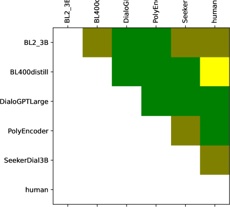
(a) Chatbot DEB

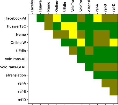
(b) WMT21 COMET

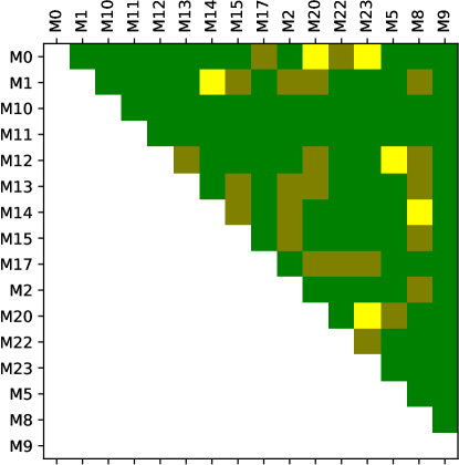
(c) SummEval Coherence Rouge

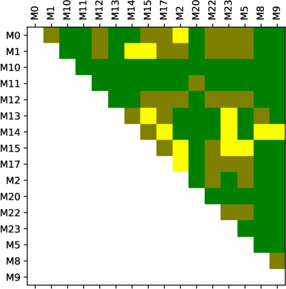
(d) SummEval Consistency BertScore

Figure 5: Pairwise Errors for the application of automated metrics with the protocol.

Appendix E Ideal Metric

Since the real-world metrics that we use in this work are not yet of very high quality, we also generated synthetic data for the SummEval-Relevance domain. That is, we simulated a metric using a fixed $\bm{\mu}_{sim}=\big{(}\begin{smallmatrix}0.8&0.25&0.1\\ 0.1&0.5&0.1\\ 0.1&0.25&0.8\\ \end{smallmatrix}\big{)}$. For this, we used the human win-rates $\bm{p}$ to randomly assign labels for each pair of system for the 11k samples. That is, for each sample, we randomly chose rating $r~{}\bm{p}$. These sampled labels are treated as the ground-truth, which has the same distribution as the human labels. Then we used $\bm{\hat{p}}=\bm{\mu}_{sim}\bm{p}$ to generate corrupted labels, which correspond to metric ratings. Since $\bm{\mu}_{sim}$ makes less mistakes than the existing metrics, and it makes no Omission or Inversion Errors. We added the ideal metric to the full results in Table 4 and 5. It also achieves a very good KLD score when applied naively. However, such a metric is currently out of scope and this only serves to illustrate an upper bound for automated metrics.

References

- Amidei et al. (2018) Jacopo Amidei, Paul Piwek, and Alistair Willis. 2018. Rethinking the agreement in human evaluation tasks. In Proceedings of the 27th International Conference on Computational Linguistics, pages 3318–3329, Santa Fe, New Mexico, USA. Association for Computational Linguistics.
- Andrieu et al. (2003) Christophe Andrieu, Nando de Freitas, Arnaud Doucet, and Michael I. Jordan. 2003. An introduction to mcmc for machine learning. 50:5–53.
- Belz et al. (2021) Anya Belz, Anastasia Shimorina, Shubham Agarwal, and Ehud Reiter. 2021. The ReproGen shared task on reproducibility of human evaluations in NLG: Overview and results. In Proceedings of the 14th International Conference on Natural Language Generation, pages 249–258, Aberdeen, Scotland, UK. Association for Computational Linguistics.
- Bingham et al. (2019) Eli Bingham, Jonathan P. Chen, Martin Jankowiak, Fritz Obermeyer, Neeraj Pradhan, Theofanis Karaletsos, Rohit Singh, Paul A. Szerlip, Paul Horsfall, and Noah D. Goodman. 2019. Pyro: Deep universal probabilistic programming. J. Mach. Learn. Res., 20:28:1–28:6.
- Brown et al. (2020) Tom Brown, Benjamin Mann, Nick Ryder, Melanie Subbiah, Jared D Kaplan, Prafulla Dhariwal, Arvind Neelakantan, Pranav Shyam, Girish Sastry, Amanda Askell, Sandhini Agarwal, Ariel Herbert-Voss, Gretchen Krueger, Tom Henighan, Rewon Child, Aditya Ramesh, Daniel Ziegler, Jeffrey Wu, Clemens Winter, Chris Hesse, Mark Chen, Eric Sigler, Mateusz Litwin, Scott Gray, Benjamin Chess, Jack Clark, Christopher Berner, Sam McCandlish, Alec Radford, Ilya Sutskever, and Dario Amodei. 2020. Language models are few-shot learners. In Advances in Neural Information Processing Systems, volume 33, pages 1877–1901. Curran Associates, Inc.
- Card et al. (2020) Dallas Card, Peter Henderson, Urvashi Khandelwal, Robin Jia, Kyle Mahowald, and Dan Jurafsky. 2020. With little power comes great responsibility. In Proceedings of the 2020 Conference on Empirical Methods in Natural Language Processing (EMNLP), pages 9263–9274, Online. Association for Computational Linguistics.
- Celikyilmaz et al. (2020) Asli Celikyilmaz, Elizabeth Clark, and Jianfeng Gao. 2020. Evaluation of text generation: A survey. arXiv preprint arXiv:2006.14799.
- Chaganty et al. (2018) Arun Chaganty, Stephen Mussmann, and Percy Liang. 2018. The price of debiasing automatic metrics in natural language evalaution. In Proceedings of the 56th Annual Meeting of the Association for Computational Linguistics (Volume 1: Long Papers), pages 643–653, Melbourne, Australia. Association for Computational Linguistics.
- Coakley and Heise (1996) Clint W. Coakley and Mark A. Heise. 1996. Versions of the sign test in the presence of ties. Biometrics, 52(4):1242–1251.
- Deriu et al. (2021) Jan Deriu, Alvaro Rodrigo, Arantxa Otegi, Guillermo Echegoyen, Sophie Rosset, Eneko Agirre, and Mark Cieliebak. 2021. Survey on evaluation methods for dialogue systems. Artificial Intelligence Review, 54(1):755–810.
- Devlin et al. (2019) Jacob Devlin, Ming-Wei Chang, Kenton Lee, and Kristina Toutanova. 2019. BERT: Pre-training of deep bidirectional transformers for language understanding. In Proceedings of the 2019 Conference of the North American Chapter of the Association for Computational Linguistics: Human Language Technologies, Volume 1 (Long and Short Papers), pages 4171–4186, Minneapolis, Minnesota. Association for Computational Linguistics.
- Domingos (2000) Pedro M. Domingos. 2000. A unified bias-variance decomposition and its applications.
- Fabbri et al. (2021) Alexander R. Fabbri, Wojciech Kryściński, Bryan McCann, Caiming Xiong, Richard Socher, and Dragomir Radev. 2021. SummEval: Re-evaluating summarization evaluation. Transactions of the Association for Computational Linguistics, 9:391–409.
- Freitag et al. (2021) Markus Freitag, Ricardo Rei, Nitika Mathur, Chi-kiu Lo, Craig Stewart, George Foster, Alon Lavie, and Ondřej Bojar. 2021. Results of the WMT21 metrics shared task: Evaluating metrics with expert-based human evaluations on TED and news domain. In Proceedings of the Sixth Conference on Machine Translation, pages 733–774, Online. Association for Computational Linguistics.
- Gao et al. (2020) Yang Gao, Wei Zhao, and Steffen Eger. 2020. SUPERT: Towards new frontiers in unsupervised evaluation metrics for multi-document summarization. In Proceedings of the 58th Annual Meeting of the Association for Computational Linguistics, pages 1347–1354, Online. Association for Computational Linguistics.
- Hashimoto et al. (2019) Tatsunori B. Hashimoto, Hugh Zhang, and Percy Liang. 2019. Unifying human and statistical evaluation for natural language generation. In North American Chapter of the Association for Computational Linguistics.
- Hoffman and Gelman (2014) Matthew D. Hoffman and Andrew Gelman. 2014. The no-u-turn sampler: Adaptively setting path lengths in hamiltonian monte carlo. Journal of Machine Learning Research, 15(47):1593–1623.
- Hovy et al. (2013) Dirk Hovy, Taylor Berg-Kirkpatrick, Ashish Vaswani, and Eduard Hovy. 2013. Learning whom to trust with MACE. In Proceedings of the 2013 Conference of the North American Chapter of the Association for Computational Linguistics: Human Language Technologies, pages 1120–1130, Atlanta, Georgia. Association for Computational Linguistics.
- Huang et al. (2020) Lishan Huang, Zheng Ye, Jinghui Qin, Liang Lin, and Xiaodan Liang. 2020. GRADE: Automatic graph-enhanced coherence metric for evaluating open-domain dialogue systems. In Proceedings of the 2020 Conference on Empirical Methods in Natural Language Processing (EMNLP), pages 9230–9240, Online. Association for Computational Linguistics.
- Humeau et al. (2020) Samuel Humeau, Kurt Shuster, Marie-Anne Lachaux, and Jason Weston. 2020. Poly-encoders: Architectures and pre-training strategies for fast and accurate multi-sentence scoring. In International Conference on Learning Representations.
- Kocmi et al. (2021) Tom Kocmi, Christian Federmann, Roman Grundkiewicz, Marcin Junczys-Dowmunt, Hitokazu Matsushita, and Arul Menezes. 2021. To ship or not to ship: An extensive evaluation of automatic metrics for machine translation. In Proceedings of the Sixth Conference on Machine Translation, pages 478–494, Online. Association for Computational Linguistics.
- Komeili et al. (2022) Mojtaba Komeili, Kurt Shuster, and Jason Weston. 2022. Internet-augmented dialogue generation. In Proceedings of the 60th Annual Meeting of the Association for Computational Linguistics (Volume 1: Long Papers), pages 8460–8478, Dublin, Ireland. Association for Computational Linguistics.
- Lin (2004) Chin-Yew Lin. 2004. ROUGE: A Package for Automatic Evaluation of Summaries. In Text Summarization Branches Out: Proceedings of the ACL-04 Workshop, pages 74–81, Barcelona, Spain. Association for Computational Linguistics.
- Lommel et al. (2014) Arle Lommel, Hans Uszkoreit, and Aljoscha Burchardt. 2014. Multidimensional quality metrics (mqm): A framework for declaring and describing translation quality metrics. Revista Tradumàtica: tecnologies de la traducció, (12):455–463.
- Lowe et al. (2017) Ryan Lowe, Michael Noseworthy, Iulian Vlad Serban, Nicolas Angelard-Gontier, Yoshua Bengio, and Joelle Pineau. 2017. Towards an automatic Turing test: Learning to evaluate dialogue responses. In Proceedings of the 55th Annual Meeting of the Association for Computational Linguistics (Volume 1: Long Papers), pages 1116–1126, Vancouver, Canada. Association for Computational Linguistics.
- Mathur et al. (2020) Nitika Mathur, Timothy Baldwin, and Trevor Cohn. 2020. Tangled up in BLEU: Reevaluating the evaluation of automatic machine translation evaluation metrics. In Proceedings of the 58th Annual Meeting of the Association for Computational Linguistics, pages 4984–4997, Online. Association for Computational Linguistics.
- Mehri and Eskenazi (2020a) Shikib Mehri and Maxine Eskenazi. 2020a. Unsupervised evaluation of interactive dialog with DialoGPT. In Proceedings of the 21th Annual Meeting of the Special Interest Group on Discourse and Dialogue, pages 225–235, 1st virtual meeting. Association for Computational Linguistics.
- Mehri and Eskenazi (2020b) Shikib Mehri and Maxine Eskenazi. 2020b. USR: An Unsupervised and Reference Free Evaluation Metric for Dialog Generation. In Proceedings of the 58th Annual Meeting of the Association for Computational Linguistics, pages 681–707, Online. Association for Computational Linguistics.
- Metropolis and Ulam (1949) Nicholas Metropolis and S. Ulam. 1949. The monte carlo method. Journal of the American Statistical Association, 44(247):335–341.
- Miller et al. (2017) A. H. Miller, W. Feng, A. Fisch, J. Lu, D. Batra, A. Bordes, D. Parikh, and J. Weston. 2017. Parlai: A dialog research software platform. arXiv preprint arXiv:1705.06476.
- Nallapati et al. (2016) Ramesh Nallapati, Bowen Zhou, Cicero dos Santos, Çağlar Gulçehre, and Bing Xiang. 2016. Abstractive text summarization using sequence-to-sequence RNNs and beyond. In Proceedings of the 20th SIGNLL Conference on Computational Natural Language Learning, pages 280–290, Berlin, Germany. Association for Computational Linguistics.
- Pang et al. (2020) Bo Pang, Erik Nijkamp, Wenjuan Han, Linqi Zhou, Yixian Liu, and Kewei Tu. 2020. Towards holistic and automatic evaluation of open-domain dialogue generation. In Proceedings of the 58th Annual Meeting of the Association for Computational Linguistics, pages 3619–3629, Online. Association for Computational Linguistics.
- Papineni et al. (2002) Kishore Papineni, Salim Roukos, Todd Ward, and Wei-Jing Zhu. 2002. Bleu: a Method for Automatic Evaluation of Machine Translation. In Proceedings of the 40th Annual Meeting of the Association for Computational Linguistics, pages 311–318, Philadelphia, Pennsylvania, USA. Association for Computational Linguistics.
- Peyrard et al. (2017) Maxime Peyrard, Teresa Botschen, and Iryna Gurevych. 2017. Learning to score system summaries for better content selection evaluation. In Proceedings of the Workshop on New Frontiers in Summarization, pages 74–84, Copenhagen, Denmark. Association for Computational Linguistics.
- Phan et al. (2019) Du Phan, Neeraj Pradhan, and Martin Jankowiak. 2019. Composable effects for flexible and accelerated probabilistic programming in numpyro. arXiv preprint arXiv:1912.11554.
- Phy et al. (2020) Vitou Phy, Yang Zhao, and Akiko Aizawa. 2020. Deconstruct to reconstruct a configurable evaluation metric for open-domain dialogue systems. In Proceedings of the 28th International Conference on Computational Linguistics, pages 4164–4178, Barcelona, Spain (Online). International Committee on Computational Linguistics.
- (37) Alec Radford, Jeffrey Wu, Rewon Child, David Luan, Dario Amodei, Ilya Sutskever, et al. Language models are unsupervised multitask learners.
- Raffel et al. (2020) Colin Raffel, Noam Shazeer, Adam Roberts, Katherine Lee, Sharan Narang, Michael Matena, Yanqi Zhou, Wei Li, and Peter J. Liu. 2020. Exploring the limits of transfer learning with a unified text-to-text transformer. Journal of Machine Learning Research, 21(140):1–67.
- Rei et al. (2020) Ricardo Rei, Craig Stewart, Ana C Farinha, and Alon Lavie. 2020. COMET: A neural framework for MT evaluation. In Proceedings of the 2020 Conference on Empirical Methods in Natural Language Processing (EMNLP), pages 2685–2702, Online. Association for Computational Linguistics.
- Sai et al. (2020) Ananya B. Sai, Akash Kumar Mohankumar, Siddhartha Arora, and Mitesh M. Khapra. 2020. Improving Dialog Evaluation with a Multi-reference Adversarial Dataset and Large Scale Pretraining. Transactions of the Association for Computational Linguistics, 8:810–827.
- Scialom et al. (2019) Thomas Scialom, Sylvain Lamprier, Benjamin Piwowarski, and Jacopo Staiano. 2019. Answers unite! unsupervised metrics for reinforced summarization models. In Proceedings of the 2019 Conference on Empirical Methods in Natural Language Processing and the 9th International Joint Conference on Natural Language Processing (EMNLP-IJCNLP), pages 3246–3256, Hong Kong, China. Association for Computational Linguistics.
- Sellam et al. (2020) Thibault Sellam, Dipanjan Das, and Ankur Parikh. 2020. BLEURT: Learning robust metrics for text generation. In Proceedings of the 58th Annual Meeting of the Association for Computational Linguistics, pages 7881–7892, Online. Association for Computational Linguistics.
- Shuster et al. (2022a) Kurt Shuster, Mojtaba Komeili, Leonard Adolphs, Stephen Roller, Arthur Szlam, and Jason Weston. 2022a. Language models that seek for knowledge: Modular search & generation for dialogue and prompt completion. arXiv preprint arXiv:2203.13224.
- Shuster et al. (2022b) Kurt Shuster, Jing Xu, Mojtaba Komeili, Da Ju, Eric Michael Smith, Stephen Roller, Megan Ung, Moya Chen, Kushal Arora, Joshua Lane, et al. 2022b. Blenderbot 3: a deployed conversational agent that continually learns to responsibly engage. arXiv preprint arXiv:2208.03188.
- Sinha et al. (2020) Koustuv Sinha, Prasanna Parthasarathi, Jasmine Wang, Ryan Lowe, William L. Hamilton, and Joelle Pineau. 2020. Learning an unreferenced metric for online dialogue evaluation. In Proceedings of the 58th Annual Meeting of the Association for Computational Linguistics, pages 2430–2441, Online. Association for Computational Linguistics.
- Smith et al. (2020) Eric Michael Smith, Mary Williamson, Kurt Shuster, Jason Weston, and Y-Lan Boureau. 2020. Can you put it all together: Evaluating conversational agents’ ability to blend skills. In Proceedings of the 58th Annual Meeting of the Association for Computational Linguistics, pages 2021–2030, Online. Association for Computational Linguistics.
- Takahashi et al. (2021) Kosuke Takahashi, Yoichi Ishibashi, Katsuhito Sudoh, and Satoshi Nakamura. 2021. Multilingual machine translation evaluation metrics fine-tuned on pseudo-negative examples for WMT 2021 metrics task. In Proceedings of the Sixth Conference on Machine Translation, pages 1049–1052, Online. Association for Computational Linguistics.
- Vasilyev et al. (2020) Oleg Vasilyev, Vedant Dharnidharka, and John Bohannon. 2020. Fill in the BLANC: Human-free quality estimation of document summaries. In Proceedings of the First Workshop on Evaluation and Comparison of NLP Systems, pages 11–20, Online. Association for Computational Linguistics.
- Vaswani et al. (2017) Ashish Vaswani, Noam Shazeer, Niki Parmar, Jakob Uszkoreit, Llion Jones, Aidan N Gomez, Lukasz Kaiser, and Illia Polosukhin. 2017. Attention is all you need. In Advances in Neural Information Processing Systems, volume 30. Curran Associates, Inc.
- Vedantam et al. (2015) Ramakrishna Vedantam, C. Lawrence Zitnick, and Devi Parikh. 2015. Cider: Consensus-based image description evaluation. In Proceedings of the IEEE Conference on Computer Vision and Pattern Recognition (CVPR).
- von Däniken et al. (2022) Pius von Däniken, Jan Deriu, Don Tuggener, and Mark Cieliebak. 2022. On the effectiveness of automated metrics for text generation systems. arXiv preprint arXiv:2210.13025.
- Walker et al. (1997) Marilyn A. Walker, Diane J. Litman, Candace A. Kamm, and Alicia Abella. 1997. PARADISE: A framework for evaluating spoken dialogue agents. In 35th Annual Meeting of the Association for Computational Linguistics and 8th Conference of the European Chapter of the Association for Computational Linguistics, pages 271–280, Madrid, Spain. Association for Computational Linguistics.
- Wei and Jia (2021) Johnny Tian-Zheng Wei and Robin Jia. 2021. The statistical advantage of automatic nlg metrics at the system level. In Annual Meeting of the Association for Computational Linguistics.
- Xu et al. (2022) Jing Xu, Arthur Szlam, and Jason Weston. 2022. Beyond goldfish memory: Long-term open-domain conversation. In Proceedings of the 60th Annual Meeting of the Association for Computational Linguistics (Volume 1: Long Papers), pages 5180–5197, Dublin, Ireland. Association for Computational Linguistics.
- Yeh et al. (2021) Yi-Ting Yeh, Maxine Eskenazi, and Shikib Mehri. 2021. A comprehensive assessment of dialog evaluation metrics. In The First Workshop on Evaluations and Assessments of Neural Conversation Systems, pages 15–33, Online. Association for Computational Linguistics.
- Zhang et al. (2019) Tianyi Zhang, Varsha Kishore, Felix Wu, Kilian Q Weinberger, and Yoav Artzi. 2019. Bertscore: Evaluating text generation with bert. arXiv preprint arXiv:1904.09675.
- Zhang et al. (2020) Yizhe Zhang, Siqi Sun, Michel Galley, Yen-Chun Chen, Chris Brockett, Xiang Gao, Jianfeng Gao, Jingjing Liu, and Bill Dolan. 2020. DIALOGPT : Large-scale generative pre-training for conversational response generation. In Proceedings of the 58th Annual Meeting of the Association for Computational Linguistics: System Demonstrations, pages 270–278, Online. Association for Computational Linguistics.