Simultaneous Position-and-Stiffness Control of Underactuated Antagonistic Tendon-Driven Continuum Robots

Abstract

Continuum robots have gained widespread popularity due to their inherent compliance and flexibility, particularly their adjustable levels of stiffness for various application scenarios. Despite efforts to dynamic modeling and control synthesis over the past decade, few studies have incorporated stiffness regulation into their feedback control design; however, this is one of the initial motivations to develop continuum robots. This paper addresses the crucial challenge of controlling both the position and stiffness of underactuated continuum robots actuated by antagonistic tendons. We begin by presenting a rigid-link dynamical model that can analyze the open-loop stiffening of tendon-driven continuum robots. Based on this model, we propose a novel passivity-based position-and-stiffness controller that adheres to the non-negative tension constraint. Comprehensive experiments on our continuum robot validate the theoretical results and demonstrate the efficacy and precision of this approach.

I Introduction

Continuum robots are a novel class of robotic systems that have made significant progress in the past few years. Their unique properties, such as scaled dexterity and mobility, make them well facilitated important and suitable for human-robot interaction and manipulation tasks in uncertain and complex environments. For example, they can be used for manipulating objects with unknown shapes, performing search and rescue operations, and whole-arm grasping [23]. By utilizing soft materials, continuum robots represent a concrete step towards developing robots with performance levels similar to those of biological organisms.

Despite the above advantages, rigid-body robots currently outperform continuum robots in tasks requiring adaptable movement and compliant interactions with the environment [14]. Consequently, many efforts have been devoted to addressing the challenges for real-time control of continuum robots that facilitate fast, efficient, and reliable operation. We refer the reader to the recent survey papers [13, 46, 40] for a comprehensive understanding of this point. The existing control approaches for soft robots can be broadly classified into two categories: data-driven (or machine learning) and model-based design. Initially, data-driven approaches dominated the research in this specific field, because obtaining reliable models of a continuum robot was believed to be overwhelmingly complex [13]. In recent years, various state-of-the-art learning methodologies have been applied to control soft robotics. These include the Koopman operator [8], Gaussian process temporal difference learning [16], supervised learning via recurrent neural networks [41], and feedforward neural networks [6]. However, it is well known that these data-driven approaches have some key limitations, including stringent requirements of data sets and no guarantee of stability or safety. Nonetheless, recent efforts from the control community have been made to impose stability constraints on models and learning policy [18, 49, 43]. On the other hand, in the last few years, the resurgence of interest in model-based control approaches has made them particularly appealing for soft robotics. This is because they are robust even when using approximate models, and possess properties that are both interpretable and manageable [13].

Unlike rigid manipulators, elastic deformation of continuum robots theoretically leads to infinite degrees-of-freedom (DoF) motion, e.g., torsion, buckling, extension, and bending. This renders them particularly suitable to be modelled by partial differential equations (PDEs) rather than conventional ordinary differential equations (ODEs) [9]. In particular, there are two prevalent categories of modelling used in this field, namely mechanics-based and geometry-based approaches. The former focuses on studying the elastic behaviour of the constitutive materials and solving the boundary conditions problem. For instance, Cosserat rod theory and Euler-Bernoulli beam theory are two methodologies for modelling commonly used in this category [44]. To enable numerical implementation of these models, they need to be solved numerically to obtain a closed formulation for each material subdomain. The finite elements method (FEM) has proven successful in the design and analysis of continuum robots with high accuracy [1]. The FEM approaches have an extremely heavy computational burden, thus not adapted to real-time control with a notable exception of [5] for quasi-static control. In contrast, geometrical models assume that the soft body can be represented by a specific geometric shape, e.g., piecewise constant curvature (PCC). As these modelling approaches often lead to kinematic models rather than dynamical models, they enable the design of kinematic or quasi-static controllers. For example, [22] provides the first exact kinematics in closed forms of trunk sections that can extend in length and bend in two dimensions, and shows how to connect workspace coordinates to actuator inputs. However, some results have shown that such types of kinematic controllers are likely to yield poor closed-loop performance [23].

To address the above-mentioned challenges, research has been conducted in the last few years on the dynamic modelling and model-based control of continuum robots. Several dynamical models have been adopted for controller synthesis of continuum robots, including the geometrically exact dynamic Cosserat model [36], port-Hamiltonian Cosserat model [9, 10], rigid-link models [21, 14], and reduced-order Euler-Lagrangian model [17, 15]; see also [7, 42] for stability analysis of equilibria in continuum robots. These works have applied various model-based constructive control approaches, such as passivity-based control (PBC) [11], partial feedback linearisation, proportional derivative (PD) control, and immersion and invariance (I&I) adaptive control. Among these, the paper [14] reports probably the earliest solution in the literature to the design and experimental validation of dynamic feedback control for soft robots.

As illustrated above, one of the primary motivations for developing continuum robots is to enable robots to showcase increased agility, adaptability, and compliant interactions. Consequently, there is an urgent and rapidly growing need to develop high-performance control algorithms to regulate position and stiffness simultaneously, particularly in certain applications involving human interaction or in complicated environments, such as search and rescue, industrial inspection, medical service, and home living care. For instance, in minimally invasive surgery, precise control of a robot’s position is crucial, and additionally, its stiffness needs to be dynamically adjusted to minimize side effects or transmit force. The problem of stiffness control, together with impedance control, is well established for rigid and softly-actuated (or articulated soft) robotics [4, 26, 30]. In contrast, the simultaneous position-and-stiffness control of continuum robots is still an open area of research. The first stiffness controller for continuum robots in the literature may refer to [28], which can be viewed as an extension of a simple Cartesian impedance controller for continuum robots using a kinematic model. In [2], the authors tailor the classic hybrid motion/force controller for a static model of multi-backbone continuum robots, and the proposed method needs the estimation of external wrenches. In [14], a Cartesian stiffness controller was proposed to achieve dynamic control of a fully-actuated soft robot, enabling interaction between the robot and its environment. Note that these works are not applicable to underactuated dynamical models of continuum robots.

This paper aims to address the above gap by proposing a novel dynamical model and a real-time control approach that regulates both position and stiffness concurrently for underactuated antagonistic tendon-driven continuum robots. The main contributions of the paper are:

• We propose a port-Hamiltonian dynamical model for a class of antagonistic tendon-driven continuum robots, which features a configuration-dependent input matrix that enables us to interpret the underlying mechanism for open-loop stiffening.

• Stiffness flexibility is one of the motivations for developing continuum robots. Using the derived underactuated dynamical model, we propose a novel potential energy shaping controller. Though simultaneous position-and-stiffness control has been widely studied for rigid and softly-actuated robots, to the best of the authors’ knowledge, this work is the first such attempt to design a controller capable of simultaneously controlling an underactuated continuum robot.

• We analyse the set of assignable equilibria for the proposed model class, which is actuated by tendons providing only non-negative tensions. Furthermore, we demonstrate how to integrate input constraints into the controller design via an input transformation.

We conducted experiments in a variety of scenarios to validate the theoretical results presented in the paper. However, due to 2) and the lack of applicable control approaches in the existing literature, we were unable to include a fair experimental comparison with previous work in this study.

The remainder of the paper is organised as follows. Section II provides a brief introduction to the proposed dynamical model of continuum robots and the problem studied in the paper. In Section III, we explain the underlying reason why the proposed model can interpret the open-loop stiffening. In Section IV we present a simultaneous position-and-stiffness controller which is further discussed in Section V. It is followed by the experimental results that were tested on a robotic platform OctRobot-I in Section VI. Finally, the paper presents some concluding remarks and discusses future work in Section VII.

Notation. All functions and mappings are assumed to be $C^{2}$-continuous. $I_{n}$ is the $n\times n$ identity matrix, $0_{n\times s}$ is an $n\times s$ matrix of zeros, the vector $\mathbf{0}_{n}$ represents $\mbox{col}(0,\ldots,0)\in\mathbb{R}^{n}$, and $\mathbf{1}_{n}:=\mbox{col}(1,\ldots,1)\in\mathbb{R}^{n}$. Throughout the paper, we adopt the convention of using bold font for variables denoting vectors, while scalars and matrices are represented in normal font. For ${\bf x}\in\mathbb{R}^{n}$, $S\in\mathbb{R}^{n\times n}$, $S=S^{\top}>0$, we denote the Euclidean norm $\|{\bf x}\|^{2}:={\bf x}^{\top}{\bf x}$, and the weighted–norm $\|{\bf x}\|^{2}_{S}:={\bf x}^{\top}S{\bf x}$. Given a function $f:\mathbb{R}^{n}\to\mathbb{R}$ we define the differential operators $\nabla f:=(\frac{\partial f}{\partial x})^{\top},\;\nabla_{x_{i}}f:=(\frac{\partial f}{\partial x_{i}})^{\top},$ where $x_{i}\in\mathbb{R}^{p}$ is an element of the vector ${\bf x}$. The set ${\cal N}$ is defined as ${\cal N}:=\{1,\ldots,n\}$. For a full rank matrix $g\in\mathbb{R}^{n\times m}$ ($m<n$), we denote the generalised inverse as $g^{\dagger}=[g^{\top}g]^{-1}g^{\top}$ and $g^{\bot}$ a full rank left annihilator. When clear from the context, the arguments of functions and mappings may be omitted.

II Model and Problem Set

II-A Modelling of A Class of Continuum Robots

In this section, we present a control-oriented rigid-link dynamical model specifically designed for a class of underactuated continuum robots driven by tendons. This model class encompasses a wide range of recently reported continuum robots in the literature, including the elephant trunk-inspired robot [51], the deployable soft robotic arm [20], the push puppet-inspired robot [3], the dexterous tip-extending robot [47], and our own developed OctRobot-I [19], alongside other notable examples [21, 12]. By employing this versatile model, we aim to provide a general framework that can effectively describe and analyse a variety of underactuated continuum robots, enabling a deeper understanding of their stiffening mechanisms and facilitating control design.

In order to visualise the modelling process, we take OctRobot-I as an example to introduce the proposed dynamical model but keep its generality in mind that the model is not limited to this specific robotic platform. This robot imitates an octopus tentacle’s structure and motion mechanism, as shown in Fig. 1. The whole continuum manipulator consists of several sections in order to be able to deform in three-dimensional space. Each of them is made of connected spine segments that are driven by a pair of cables. More details of the continuum robot OctRobot-I are given in Section VI-A, as well as in [19].

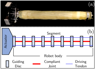
Figure 1: (a) A photo of the continuum robot OctRobot-I (b) Mechanical structure of a class of continuum robots

In this paper, we use a rigid-link model to approximate the dynamical behaviours of continuum robots for three reasons: 1) the considered class of continuum robots naturally partitions into spine segments; 2) rigid-link models simplify control-oriented tasks; and 3) it is convenient to account for external loading.

To obtain the dynamical model, we make the following assumptions.

Assumption 1

The continuum robot satisfies the properties:

• The actuator dynamics is negligible, i.e., the motor is operating in the torque control mode with sufficiently short transient stages;

• The sections have a piecewise constant curvature, conforming to the segments. $\triangleleft$

Assumption 2

The axial stiffness $K_{\tt A}$ at the end-effector is infinite, i.e. $K_{\tt A}\to\infty$. In other words, the continuum robot is axially inextensible. $\triangleleft$

In this paper, we specifically concentrate on the two-dimensional case, limiting our analysis to a single section, in order to effectively illustrate the underlying mechanism.

In the rigid-link dynamical model, we use a serial chain of rigid links with $n$ rotational joints to approximate one section of the continuum robot. Then, the configuration variable can be defined as

$${\bf q}=\begin{bmatrix}q_{1}&\ldots&q_{n}\end{bmatrix}^{\top}\in{\cal X}\subset\mathbb{R}^{n},$$

with $q_{i}$ representing the approximate link angles, where ${\cal X}$ is the feasible configuration space; see Fig. 2 for an illustration. Practically, all angles $q_{i}$ are within some subsets of $[-{\pi\over 2},{\pi\over 2}]$ due to physical constraints.

We model the continuum robot as a port-Hamiltonian system in the form of [31, 45]

$$\begin{bmatrix}~{}\dot{\bf q}~{}\\ ~{}\dot{\bf p}~{}\end{bmatrix}=\begin{bmatrix}0_{n\times n}&I_{n}\\ -I_{n}&-D({\bf q})\end{bmatrix}\begin{bmatrix}\nabla_{{\bf q}}H\\ \nabla_{{\bf p}}H\end{bmatrix}+\begin{bmatrix}~{}\mathbf{0}_{n}~{}\\ ~{}G({\bf q}){\bf u}+\tau_{\tt ext}~{}\end{bmatrix}$$ (1)

with the generalised momenta ${\bf p}\in\mathbb{R}^{n}$, the damping matrix $D({\bf q})\in\mathbb{R}^{n\times n}_{\succ 0}$, $\tau_{\tt ext}\in\mathbb{R}^{n}$ the external torque, and the input matrix $G({\bf q})\in\mathbb{R}^{n\times m}$ with $m<n$. The total energy of the robotic system is given by

$$H({\bf q},{\bf p})={1\over 2}{\bf p}^{\top}M^{-1}({\bf q}){\bf p}+U({\bf q}),$$ (2)

with the inertia matrix $M({\bf q})\succ 0$, and the potential energy $U({\bf q})$, which consists of the gravitational part $U_{\tt G}$ and the elastic one $U_{\tt E}({\bf q})$, i.e.

$$U({\bf q})~{}=~{}U_{\tt G}({\bf q})+U_{\tt E}({\bf q}).$$

The potential energy function has an isolated local minimum at its open-loop equilibrium ${\bf q}=\mathbf{0}_{n}$.

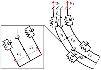
Figure 2: An illustration of configuration variables (The symbol “$\bullet$” indicates the lumped mass $m_{i}$; the angle $q_{i}$ assumes positive values for small counter-clockwise rotations.)

Fig. 2 shows the above rigid-link model of continuum robots. Similar to [14], we adopt the assumption that a lumped mass with the value $m_{i}~{}(i\in{\cal N})$ is virtually placed in the middle of each link, and the link lengths are $\ell_{i}$. We additionally make the following assumption on the mass and length.

Assumption 3

The continuum robot satisfies the uniformity assumptions:

• The masses verify $m_{i}=m_{j},~{}\forall i,j\in{\cal N}.$

• The lengths satisfy the relation: $l_{0}=\ell$ and $l_{i}=2\ell$ ($i\in{\cal N}$) for some $\ell>0$. The radius of the beam is $r$. $\triangleleft$

The gravitational and elastic potential energy functions $U_{\tt G},U_{\tt E}$ can be derived according to the geometric deformation under the uniformity assumptions of the materials. To make the paper self-contained, the details on the modelling of the potential energy functions are given in Appendix.

The variable ${\bf u}\in\mathbb{R}^{m}$ represents the control input, denoting the tensions along the cables generated by actuators. In particular, in the planar case, we have $m=2$ with two cables. Due to the specific structure, these two tensions are one-directional, i.e.,

$$u_{i}\geq 0\quad(i=1,2).$$ (3)

For the studied case, the input matrix $G({\bf q}):\mathbb{R}^{n}\to\mathbb{R}^{n\times 2}$ can be conformally partitioned as

$$G({\bf q})~{}=~{}\begin{bmatrix}~{}G_{1}({\bf q})&G_{2}({\bf q})~{}\end{bmatrix}.$$ (4)

In the following assumption, some key properties of the matrix $G({\bf q})$ are underlined when modelling the continuum robot.

Assumption 4

The input matrix $G({\bf q})$ of the continuum robot model (1) – or equivalently in (4) – satisfies

• $G({\bf q})$ is state-dependent and $C^{1}$-continuous.

• $G_{1}(\textbf{0}_{n})=-G_{2}(\textbf{0}_{n})$.

• $\|G_{1}({\bf q})+G_{2}({\bf q})\|\neq 0$ for ${\bf q}\in{{\cal X}}\backslash\{\textbf{0}_{n}\}$. $\triangleleft$

Among the above three items, the state-dependency of the input matrix is a key feature of the proposed model, which is instrumental in showing the tunability of open-loop stiffness of tendon-driven continuum robots. We will give more details about the input matrix in the subsequent sections of the paper. The second point (b) means that at the open-loop equilibrium (i.e. ${\bf q}=\textbf{0}_{n}$), the tensions in the two cables are equal in magnitude but opposite in direction.

Remark 1

Let us now consider a single link in the zoomed-in subfigure in Fig. 2. If the forces along the cables are assumed lossless, their directions are nonparallel to the centroid of the continuum robot. The torques imposed on the first approximate link are given by $u_{1}\mathcal{L}_{1}(q_{1})$ and $u_{2}{\cal L}_{2}(q_{1})$ with $\mathcal{L}_{1},\mathcal{L}_{2}$ the lever’s fulcrums, which are nonlinear functions of the configuration $q_{1}$. From some basic geometric relations, it satisfies ${\cal L}_{1}(0)={\cal L}_{2}(0)$. This illustrates the rationality of Assumption 4. $\triangleleft$

II-B Problem Set

In this paper, we study how to design a feedback controller that is capable of regulating the continuum robot deformation and achieving the variable stiffness capability. To be precise, the closed loop complies with the input constraint (3) and achieves the following aims:

• In the absence of the external torque (i.e. $\tau_{\tt ext}=\mathbf{0}_{n}$), it achieves the asymptotically accurate regulation of the position, that is

  $$\lim_{t\to\infty}{\bf q}(t)={\bf q}_{\star},$$ (5)

  with a desired assignable configuration ${\bf q}_{\star}\in{\cal X}$.

• We are able to control the stiffness at the closed-loop equilibrium concurrently.

III Open-loop Stiffening

It is widely recognised that the antagonism mechanism is a popular method for stiffening of tendon-driven continuum robots [20]. By arranging a pair of cables on two sides of the robot and adjusting their tensions simultaneously, the robot body compresses or expands, and generates a reaction that counteracts the tension. As a consequence, the stiffness of the robot changes.

In this section, it is shown, via an intuitive example, that there is a redundant degree of freedom of input in the proposed model, which provides the possibility to regulate the stiffness in the open-loop system. This property is instrumental for the controller design to regulate position and stiffness simultaneously.

Now consider the case of the open-loop system with a pair of identical constant inputs

$$u_{1}=u_{2}=\mu.$$ (6)

This balance will keep the configuration variable ${\bf q}$ at the open-loop equilibrium ${\bf q}_{\star}=\mathbf{0}_{n}$ for any feasible $\mu\geq 0$. Especially, when $\mu=0$, the robot is in a slack state where its stiffness corresponds to its inherent properties determined by the materials and mechanical structures. Intuitively, as $\mu$ increases, the manipulator progressively transitions towards a state of higher rigidity or inflexibility. The proposed dynamical model should be capable of interpreting the above phenomenon – physical common senses tell us that a larger value of $\mu>0$ implies a larger transverse stiffness.

In order to study the stiffness at the end-effector, we need the Jacobian $J({\bf q})\in\mathbb{R}^{2\times n}$ from the contact force ${\bf f}_{\tt ext}\in\mathbb{R}^{2}$, i.e., satisfying

$$\tau_{\tt ext}=J^{\top}({\bf q}){\bf f}_{\tt ext},$$ (7)

in which $\tau_{\tt ext}\in\mathbb{R}^{n}$ is the external torque vector acting on each link.

In the following proposition, we aim to demonstrate the property of stiffness tunability by changing the value $\mu$ in the proposed dynamical model.

Proposition 1

Consider the antagonistic tendon-driven model (1) for continuum robots, with the constant inputs (6) under Assumption 4. If the following assumptions are satisfied:

• For $j=1,2$

  $${\partial G_{n,j}\over\partial q_{n}}({\bf q})<0,$$ (8)

  $${\partial G_{n,j}\over\partial q_{k}}({\bf q})=0,~{}k\in{\cal N}\backslash\{n\}$$

  in a neighbourhood of the origin.

• The forward kinematics (the mapping from the configuration ${\bf q}\in{\cal X}$ to the end-effector Cartesian coordinate ${\bf x}\in\mathbb{R}^{2}$) is a locally injective immersion.

Then, the input (6) guarantees the origin $\mathbf{0}_{n}$ an equilibrium in the absence of the external perturbation, i.e. $\tau_{\tt ext}=\mathbf{0}$. Furthermore, a large input value $\mu>0$ implies a larger transverse stiffness $K_{\tt T}$ of the end-effector at this open-loop equilibrium.

Proof:

From Assumption 4(b), the input term

$$G({\bf q}){\bf u}\big{|}_{{\bf q}=\mathbf{0}_{n}}=\mathbf{0}_{n}$$

with (6) guarantees that the origin ${\bf q}_{\star}=\mathbf{0}_{n}$ is an equilibrium in the case of $\tau_{\tt ext}=\mathbf{0}$.

The Cartesian coordinate ${\bf x}\in\mathbb{R}^{2}$ of the end-effector can be uniquely determined by the configuration ${\bf q}$ as

$${\bf x}=T({\bf q})$$ (9)

for some smooth function $T:\mathbb{R}^{n}\to\mathbb{R}^{2}$, with the open-loop equilibrium ${\bf x}_{\star}:=T({\bf q}_{\star})$. Note that the function $T$ depends on the coordinate selection. Without loss of generality, we assume ${\bf x}_{\star}=\mathbf{0}_{2}$ and the local coordinate of ${\bf x}:=\mbox{col}(x_{1},x_{2})$ are selected as the tangential and the axial directions of the $n$-th link.

For a non-zero constant $\tau_{\tt ext}$, let us denote the shifted equilibrium as $(\bar{\bf q},\mathbf{0}_{n})$ in the presence of the external perturbation, with the corresponding end-effector coordinate $\bar{\bf x}=T(\bar{\bf q}).$

In order to study the transverse stiffness at the end of the robot, we assume that the external force ${\bf f}_{\tt ext}$ is only applied to the $n$-th link [38]. Substituting it into the port-Hamiltonian model (1), it satisfies the following equations at the shifted equilibrium

$$\nabla U(\bar{\bf q}) ~{}=~{}[G_{1}(\bar{\bf q})+G_{2}(\bar{\bf q})]\mu+J^{\top}(\bar{\bf q}){\bf f}_{\tt ext}$$ (10)

$${\bf f}_{\tt ext} ~{}=~{}K_{\tt C}(\bar{\bf x}-{\bf x}_{\star}),$$

in which $K_{\tt C}\in\mathbb{R}^{2\times 2}$ is the stiffness matrix with the partition

$$K_{\tt C} :=\mbox{diag}(K_{\tt T},K_{\tt A})$$

with

$$J({\bf q})=\begin{bmatrix}J_{1}({\bf q})\\ J_{2}({\bf q})\end{bmatrix},$$

the axial stiffness $K_{\tt A}$ and the transverse stiffness $K_{\tt T}$. For the particular coordinate selection as mentioned above, the Jacobian matrix $J_{1}({\bf q})$ is in the form

$$J_{1}=\begin{bmatrix}0&\ldots&0&l_{n}\end{bmatrix},$$ (11)

in which $l_{n}>0$ represents the distance from the contact point to the centre of the $n$-th link.

From Assumption 2, the continuum robot is inextensible along the axial direction, which implies $\bar{x}_{2}-{x_{\star}}_{2}=0.$ Hence, we have

$$\nabla U(\bar{\bf q})=[G_{1}(\bar{\bf q})+G_{2}(\bar{\bf q})]\mu+K_{\tt T}J_{1}^{\top}\left[\bar{x}_{1}-x_{\star 1}\right].$$ (12)

For convenience of presentation and analysis, we define a function $f_{\mu}:\mathbb{R}^{n}\to\mathbb{R}^{n}$ as

$$f_{\mu}({\bf q}):=\nabla U({\bf q})-[G_{1}({\bf q})+G_{2}({\bf q})]\mu,$$ (13)

which is parameterised by the constant force $\mu\geq 0$. Invoking the fact that ${\bf q}_{\star}=\mathbf{0}_{n}$ is an open-loop equilibrium, we have

$$f_{\mu}({\bf q}_{\star})=0,$$ (14)

and thus

$$f_{\mu}(\bar{\bf q})-f_{\mu}({\bf q}_{\star})=K_{\tt T}J_{1}^{\top}(\bar{\bf q})[\bar{x}_{1}-x_{\star 1}].$$ (15)

Noting the local injectivity assumption H2, there exists a left inverse function $T^{\tt L}$ – which is defined locally – of the function $T$ such that

$${\bf q}=T^{\tt L}(T({\bf q}))$$ (16)

in a small neighborhood of ${\bf q}_{\star}$.

From the equation (15), the transverse stiffness $K_{\tt T}$ at the open-loop equilibrium ${\bf q}_{\star}$ can be defined by taking the limit $\bar{\bf q}\to{\bf q}_{\star}$, i.e.

$$K_{\tt T} ~{}=~{}{J_{1}({\bf q}_{\star})\over\|J_{1}({\bf q}_{\star})\|^{2}}\lim_{\bar{x}_{1}\to x_{\star 1}}{f_{\mu}(\bar{\bf q})-f_{\mu}({\bf q}_{\star})\over\bar{x}_{1}-x_{\star 1}}$$ (17)

$$~{}=~{}{J_{1}({\bf q}_{\star})\over\|J_{1}({\bf q}_{\star})\|}^{2}[\nabla f_{\mu}({\bf q}_{\star})]^{\top}\nabla_{x_{1}}T^{\tt L}({\bf x}_{\star})$$

$$~{}=~{}{J_{1}\over\|J_{1}\|}^{2}\big{[}\nabla^{2}U-\mu\big{(}\nabla G_{1}+\nabla G_{2}\big{)}^{\top}\big{]}\nabla_{x_{1}}T^{\tt L}\bigg{|}_{{\bf q}_{\star}}.$$

The assumption H1 guarantees that the $(n,n)$-element of $\nabla G_{j}({\bf q}_{\star})$ for $j=1,2$ is negative. On the other hand, from the local coordinate selection, the variation of $x_{1}$ implies that $q_{n}$ will also change accordingly. As a consequence, the last element of $\nabla_{x_{1}}T^{\tt L}$ is non-zero, and indeed, it is positive. It is straightforward to see that $K_{\tt T}$ is increasing by selecting a larger $\mu>0$. $\triangleleft$

With the proposed dynamical model, the above calculation shows the underlying mechanism of the tunability of open-loop stiffness. Later on, we will illustrate that the tension difference $(u_{1}-u_{2})$ provides another degree of freedom to regulate the robot configuration.

Remark 2

Assumption H1 means that $G_{n,j}$ only depends on the state $q_{n}$ rather than other configuration variables. It is used to simplify the presentation and analysis. Indeed, from the above proof, it may be replaced by a weaker condition $J_{1}(\nabla G_{1}+\nabla G_{2})\nabla_{x_{1}}T^{\tt L}\neq 0$, for which we are still able to show the ability to tune the open-loop stiffness via changing the tendon force $\mu$. The assumption H2 means that we can determine a unique inverse kinematic solution in a small neighborhood of a given configuration ${\bf q}_{\star}$. While it is generally not true to ensure the existence of a global inverse, achieving it within a local context is feasible.

Remark 3

In practice, when the value $\mu$ is increased beyond a certain threshold, the continuum robot may be observed with the phenomenon of buckling [18, Sec. III]. However, the critical values are usually very large, and cannot be generated by actuators in many robotic platforms. In this paper, we do not take the buckling behaviour into account.

IV Control Design

In this section, we will study how to design a state feedback law, based on the proposed model in Section II, to regulate position and stiffness simultaneously.

To facilitate the controller design, we additionally assume the following for the input matrix $G({\bf q})$ in terms of the geometric constraints.

Assumption 5

The matrix $G({\bf q})$ given by (4) is reparameterised as

$$G_{1}({\bf q}) ~{}=~{}\mathbf{g}_{1}({\bf q})+\mathbf{g}_{0}$$ (18)

$$G_{2}({\bf q}) ~{}=~{}\mathbf{g}_{1}({\bf q})-\mathbf{g}_{0}$$

with a constant vector $\mathbf{g}_{0}\in\mathbb{R}^{n}$ and a $C^{1}$-continuous function $\mathbf{g}_{1}:\mathbb{R}^{n}\to\mathbb{R}^{n}$ satisfying the following:

• $\mathbf{g}_{1}({\bf q})$ is a smooth odd function;

• $\mathbf{g}_{1}({\bf q})$ is full column rank for ${\bf q}\in{\cal X}/\{\mathbf{0}_{n}\}$;

• The constant vector $\mathbf{g}_{0}$ and the vector field $\mathbf{g}_{1}({\bf q})$ can be re-parameterised as

  $$\mathbf{g}_{0}=g_{0}\mathbf{1}_{n},\quad\mathbf{g}_{1}({\bf q})=g_{1}({\bf q})\mathbf{1}_{n},$$ (19)

  and $g_{0}+g_{1}({\bf q})\neq 0$ for all ${\bf q}$. $\triangleleft$

Clearly, the above is compatible with Assumption 4. The vector-valued function $\mathbf{g}_{1}({\bf q})$ is related to the open-loop stiffness tunability outlined in Proposition 1. At the end of Appendix, we provide some details on how to model the terms $g_{0}$ and $g_{1}$.

IV-A Assignable Equilibria

For underactuated mechanical systems, it is essential to identify the set of assignable equilibria, also referred to as achievable or feasible equilibria. Although this has been extensively explored, tendon-driven robots face a significant obstacle in the form of the one-directional input constraint (3).

In order to facilitate the control design, we make the following input transformation:

$$\tau=T_{\tt u}{\bf u},\quad T_{\tt u}:=\begin{bmatrix}1&-1\\ 0&1\end{bmatrix}$$ (20)

with new input control

$$\tau=\mbox{col}(\tau_{1},\;\tau_{2})\in\mathbb{R}^{2}.$$

For $\tau_{1}$, there is no sign constraint; the other input channel verifies $\tau_{2}\geq 0$, and thus we define the admissible input set as

$${\cal E}_{\tau}:=\{\tau\in\mathbb{R}^{2}:\tau_{1}\in\mathbb{R},~{}\tau_{2}\geq 0\}.$$ (21)

Invoking the intuitive idea in Section III, we may use these two inputs $\tau_{1},\tau_{2}$ to regulate the position and stiffness concurrently.

For convenience, we define the new input matrix as

$$G_{\tau}({\bf q})=\begin{bmatrix}\rho_{1}({\bf q})&\rho_{2}({\bf q})\end{bmatrix}=:G({\bf q})T_{\tt u}^{-1}$$ (22)

with

$$\rho_{1}({\bf q}) ~{}=~{}\mathbf{g}_{0}+\mathbf{g}_{1}({\bf q})$$

$$\rho_{2}({\bf q}) ~{}=~{}2\mathbf{g}_{1}({\bf q}).$$

With the above input transformation, the controlled model (1) now becomes

$$\begin{bmatrix}~{}\dot{\bf q}~{}\\ ~{}\dot{\bf p}~{}\end{bmatrix}=\begin{bmatrix}0_{n\times n}&I_{n}\\ -I_{n}&-D({\bf q})\end{bmatrix}\begin{bmatrix}\nabla_{{\bf q}}H\\ \nabla_{{\bf p}}H\end{bmatrix}+\begin{bmatrix}~{}\mathbf{0}_{n}~{}\\ ~{}G_{\tau}({\bf q})\tau~{}\end{bmatrix}$$ (23)

in the absence of the external perturbation $\tau_{\tt ext}$.

Remark 4

Indeed, the real constraint for $\tau_{1}$ should be $\tau_{1}\geq-\tau_{2}$ rather than $\tau_{1}\in\mathbb{R}$ in order to guarantee the constraint $u_{1},u_{2}\geq 0$. Since we are able to set the value of $\tau_{2}$ arbitrarily, we consider the admissible input set ${\cal E}_{\tau}$ defined above for convenience in the subsequent analysis. $\triangleleft$

According to [31] and invoking the full rankness of $T_{u}$, if there were not input constraints, the assignable equilibrium set would be given by $\{{\bf q}\in\mathbb{R}^{n}:G({\bf q})^{\bot}\nabla U({\bf q})=\mathbf{0}\}.$ Clearly, this does not hold true for our case, because the feasible solution cannot be guaranteed to live within the set ${\cal E}_{\tau}$ rather than $\tau\in\mathbb{R}^{2}$.

To address this point, in the following proposition we present the assignable equilibria set for the studied case with constrained inputs.

Proposition 2

(Assignable Equilibria) Consider the unperturbed model (1) and the input transformation (20) with $\tau_{\tt ext}=\mathbf{0}$ under the input constraint ${\cal E}_{\tau}$ in (21). All the assignable equilibria are given by the set ${\cal E}_{q}\cap{\cal X}$, with the definition

$${\cal E}_{q}:=$$

$$~{}~{}~{}~{}\left\{{\bf q}\in\mathbb{R}^{n}\Bigg{|}\begin{aligned} (\mathbf{g}_{1}^{\bot}\mathbf{g}_{0})^{\bot}\mathbf{g}_{1}^{\bot}\nabla U=0\\ \mathbf{g}_{1}^{\top}\nabla U-\mathbf{g}_{1}^{\top}(\mathbf{g}_{0}+\mathbf{g}_{1})(\mathbf{g}_{1}^{\bot}\mathbf{g}_{0})^{\dagger}\mathbf{g}_{1}^{\bot}\nabla U\geq 0\end{aligned}\right\}.$$

Proof:

In terms of Assumption 5(b), we can always find a left annihilator $\mathbf{g}_{1}^{\bot}({\bf q})\in\mathbb{R}^{(n-1)\times n}$, which is full rank for all ${\bf q}\in{\cal X}/\{\mathbf{0}_{n}\}$. For an equilibrium $({\bf q},{\bf 0})$, there should exist $\tau_{1}$ and $\tau_{2}$ satisfying

$$\nabla U({\bf q}) ~{}=~{}G_{\tau}({\bf q})\tau$$ (24)

$$~{}=~{}[\mathbf{g}_{0}+\mathbf{g}_{1}({\bf q})]\tau_{1}+2\mathbf{g}_{1}({\bf q})\tau_{2}.$$

Considering the full-rankness of the square matrix

$$\begin{bmatrix}~{}\mathbf{g}_{1}^{\bot}({\bf q})~{}\\ ~{}\mathbf{g}_{1}^{\top}({\bf q})~{}\end{bmatrix}\in\mathbb{R}^{n\times n}$$

for ${\bf q}\in{\cal X}/\{\mathbf{0}_{n}\}$, we have

$$\eqref{id:eq1}~{}\iff~{}\begin{bmatrix}\mathbf{g}_{1}^{\bot}\\ \mathbf{g}_{1}^{\top}\end{bmatrix}\nabla U=\begin{bmatrix}\mathbf{g}_{1}^{\bot}\mathbf{g}_{0}\tau_{1}\\ \mathbf{g}_{1}^{\top}(\mathbf{g}_{0}+\mathbf{g}_{1})\tau+2\|\mathbf{g}_{1}\|^{2}\tau_{2}\end{bmatrix}.$$ (25)

Its solvability relies on finding all the points ${\bf q}\in{\cal X}\subset\mathbb{R}^{n}$ satisfying

$$\mathbf{g}_{1}^{\bot}\nabla U =\mathbf{g}_{1}^{\bot}\mathbf{g}_{0}\tau_{1}$$ (26)

$$\mathbf{g}_{1}^{\top}\nabla U =\mathbf{g}_{1}^{\top}(\mathbf{g}_{0}+\mathbf{g}_{1})\tau_{1}+2\|\mathbf{g}_{1}\|^{2}\tau_{2}$$ (27)

at the same time under the constraint $\tau\in{\cal E}_{\tau}$. Clearly, all the feasible equilibria satisfying (26) live in the set

$$\{{\bf q}\in\mathbb{R}^{n}:(\mathbf{g}_{1}^{\bot}({\bf q})\mathbf{g}_{0})^{\bot}\mathbf{g}_{1}^{\bot}({\bf q})\nabla U({\bf q})=0\},$$

and the corresponding input $\tau_{1}$ is given by

$$\tau_{1}=(\mathbf{g}_{1}^{\bot}\mathbf{g}_{0})^{\dagger}\mathbf{g}_{1}^{\bot}\nabla U.$$ (28)

On the other hand, Assumption 5(b) imposes the constraint $\|\mathbf{g}_{1}\|^{2}>0$, thus (27) admits a positive solution to $\tau_{2}\geq 0$ if and only if

$$\mathbf{g}_{1}^{\top}\nabla U-\mathbf{g}_{1}^{\top}(\mathbf{g}_{0}+\mathbf{g}_{1})\tau_{1}\geq 0.$$ (29)

Inserting (28) into the above equation completes the proof. $\triangleleft$

After imposing Assumption 5(c) to the input matrix $G({\bf q})$, we are interested in a class of particular equilibria. In this paper, we call them the homogeneous equilibria that are characterised by the set

$${\cal E}_{\theta}:=\{{\bf q}\in\mathbb{R}^{n}:q_{i}=\theta,~{}\forall i\in{\cal N}\}$$ (30)

for some constant $\theta$. This definition is tailored for the proposed continuum robot model under the assumptions in the paper.

In the following, we show all homogeneous equilibria belong to the assignable equilibrium set ${\cal E}_{q}$ in Proposition 2.

Proposition 3

Consider the model (1) of the continuum robot under Assumptions 5-7. Then, all homogeneous equilibria are assignable, i.e. ${\cal E}_{\theta}\subset{\cal E}_{q}$.

Proof:

For the case with $\theta=0$, since $g_{1}(\mathbf{0}_{n})=0$, the equilibrium ${\bf q}_{\star}=\theta\mathbf{1}_{n}$ makes the equation (24) solvable with $\tau_{1}=0$ and any $\tau_{2}\geq 0$.

For the case with $\theta\neq 0$ and any fixed $\tau_{1}\geq 0$, the determination of the set ${\cal E}_{q}$ is equivalent to solving (24), which can be written as

$$\nabla U({\bf q})=[\mathbf{g}_{0}+\mathbf{g}_{1}({\bf q})]\tau_{1}+2\mathbf{g}_{1}({\bf q})\tau_{2}.$$

We compactly formulate the above as

$$\nabla U({\bf q})=G_{\tt N}\tau_{\tt N}$$ (31)

with the new definitions

$$G_{\tt N} ~{}:=~{}\mathbf{1}_{n}$$ (32)

$$\tau_{\tt N}(\tau) ~{}:=~{}[g_{0}+g_{1}({\bf q})]\tau_{1}+2g_{1}({\bf q})\tau_{2}.$$

For any fixed $\tau_{2}\geq 0$, invoking (19) from Assumption 5, the mapping $\tau_{1}\to\tau_{\tt N}$ is a diffeomorphism from $\mathbb{R}\to\mathbb{R}$. It implies that there is no constraint for $\tau_{\tt N}$. As a consequence, the PDE (31) becomes

$$G_{\tt N}^{\bot}\nabla U({\bf q}_{\star})=0$$ (33)

at the desired equilibrium ${\bf q}_{\star}$.

A feasible full-rank annihilator of $G_{\tt N}$ is given by

$$G_{\tt N}^{\bot}=\begin{bmatrix}1&-1&0&\ldots&0\\ 0&1&-1&\ldots&0\\ &&\ddots&\ddots\\ 0&\ldots&0&1&-1\end{bmatrix}\in\mathbb{R}^{(n-1)\times n},$$ (34)

and the Jacobian $\nabla U$ at the desired equilibrium ${\bf q}_{\star}$ is in the form

$$\nabla U({\bf q}_{\star})=\alpha_{1}\underbrace{\begin{bmatrix}~{}\sin(q_{\Sigma})~{}\\ \vdots\\ ~{}\sin(q_{\Sigma})~{}\end{bmatrix}}_{\sin(n\theta)\mathbf{1}_{n}}+\alpha_{2}\underbrace{\begin{bmatrix}~{}{\bf q}_{\star,1}~{}\\ ~{}\vdots~{}\\ ~{}{\bf q}_{\star,n}~{}\end{bmatrix}}_{\theta\mathbf{1}_{n}}$$ (35)

with

$$q_{\Sigma}:=\sum_{i\in{\cal N}}{\bf q}_{i}.$$

It is straightforward to verify that (33) holds true for any $\tau_{2}\geq 0$ with a homogeneous equilibrium ${\bf q}_{\star}=\theta\mathbf{1}_{n}$. Since there is no constraint for the input variable $\tau_{1}$, the equilibrium for this case is also assignable under the constraint (21). We complete the proof. $\triangleleft$

In the sequel of the paper, our focus will be on control algorithm design aimed at regulating certain homogeneous equilibria that have been demonstrated to be assignable within the proposed class of models for continuum robots.

IV-B Simultaneous Position-and-Stiffness Control

We now aim at stabilising an arbitrary homogeneous equilibrium ${\bf q}_{\star}$ in the subset of ${\cal E}_{\theta}$ with a tunable stiffness of the closed loop.

Towards the end, we will employ the passivity-based control (PBC) method since it has a clear energy interpretation and simplifies both modelling and controller design. This makes it suitable for continuum robots to preserve the system compliance [21].

Our basic idea is to fix $\tau_{2}$ at some constant value $\tau_{2}^{\star}\geq 0$. We then utilise the input $\tau_{1}$ to achieve potential energy shaping for the regulation task. Compared to the more general approach of interconnection and damping assignment (IDA) PBC [32], on one hand, potential energy shaping may provide a simpler controller form, and on the other hand, as pointed out in [24] changing the inertia is prone to fail in practice – albeit being theoretically sound with additional degrees of freedom.

For a given input $\tau_{2}=\tau_{2}^{\star}\geq 0$, the actuation into the dynamics is given by

$$G_{\tau}({\bf q})\tau ~{}=~{}\rho_{1}({\bf q})\tau_{1}+\rho_{2}({\bf q})\tau_{2}^{\star}$$ (36)

$$:=~{}G_{\tt N}\tau_{\tt N}(\mbox{col}(\tau_{1},\tau_{2}^{\star})),$$

with the function $\tau_{\tt N}:\mathbb{R}^{2}\to\mathbb{R}$ defined in (32). From Assumption 5, the vector field $\rho_{1}({\bf q})\neq 0$ for all ${\bf q}\in{\cal X}$. Now the design target becomes using the control input $\tau_{1}$ (with a fixed $\tau_{2}^{\star}$) to shape the potential energy function $U({\bf q})$ into a new one – the desired potential energy function $U_{\tt d}({\bf q})$. To this end, we need to solve the PDE [31]

$$G_{\tt N}^{\bot}\big{[}\nabla U({\bf q})-\nabla U_{\tt d}({\bf q})\big{]}=0.$$ (37)

Note that the solution to the function $U_{\tt d}$ must adhere to the constraints

$$\nabla U_{\tt d}({\bf q}_{\star}) ~{}=~{}0$$ (38)

$$\nabla^{2}U_{\tt d}({\bf q}_{\star}) ~{}\succ~{}0,$$ (39)

in order to make the desired configuration ${\bf q}_{\star}$ an asymptotically stable equilibrium.

We are now in the position to propose the controller for simultaneous control of position and stiffness.

Proposition 4

Consider the continuum robotic model (1), (20) with the constraint (21) satisfying Assumptions 4-7, and the full-rank damping matrix $D({\bf q})$ is uniformly positive definite. The feedback controller

$$u=T_{u}^{-1}\tau$$ (40)

with the transformed input

$$\tau=\tau_{\tt es}+\tau_{\tt da}+\tau_{\tt st}$$ (41)

and the terms

$$\tau_{\tt st} =\begin{bmatrix}-{2g_{1}({\bf q})\over g_{0}+g_{1}({\bf q})}\\ 1\end{bmatrix}\tau_{2}^{\star}$$ (42)

$$\tau_{\tt es} =\begin{bmatrix}{1\over g_{0}+g_{1}({\bf q})}G_{\tt N}^{\dagger}(\nabla U_{\tt d}-\nabla U)\\ 0\end{bmatrix}$$

$$\tau_{\tt da} =\begin{bmatrix}-{1\over g_{0}+g_{1}({\bf q})}G_{\tt N}^{\top}K_{\tt d}M^{-1}({\bf q}){\bf p}\\ 0\end{bmatrix},$$

where $G_{\tt N}=\mathbf{1}_{n}$, $\tau_{2}^{\star}>0$, $K_{\tt d}\succ 0$ is a gain matrix, and the desired potential energy function is given by

$$U_{\tt d}({\bf q}) ~{}=~{}-\gamma\cos(q_{\Sigma}-q_{\Sigma}^{\star})+{\alpha_{2}\over 2}\|{\bf q}-{\bf q}_{\star}\|^{2}$$ (43)

$$q_{\Sigma}^{\star} ~{}=~{}\sum_{i\in{\cal N}}{\bf q}_{\star,i},$$

the gain $\gamma>0$, and some desired regulation configuration ${\bf q}_{\star}\in{\cal E}_{\theta}$, achieves the following closed-loop properties:

• (Position regulation in free motion) If the external force $\tau_{\tt ext}=0$ and $\gamma<\alpha_{2}$, then the desired equilibrium point ${\bf q}_{\star}$ is globally asymptotically stable (GAS) with

  $$\lim_{t\to+\infty}{\bf q}(t)={\bf q}_{\star}.$$ (44)

• (Compliant behavior) The overall closed-loop stiffness (i.e., from the external torque $\tau_{\tt ext}\in\mathbb{R}^{n}$ to the configuration ${\bf q}\in\mathbb{R}^{n}$) is

  $$K_{\tt O}=\gamma\mathbf{1}_{n\times n}+\alpha_{2}I_{n},$$ (45)

  where $\mathbf{1}_{n\times n}$ is an $n\times n$ matrix of ones. $\triangleleft$

Proof:

First, it is straightforward to verify that the vector $\tau_{\tt st}$ in (42) is in the null space of $\tau_{\tt N}(\tau)$ for any $\tau_{2}^{\star}$, i.e.,

$$\tau_{\tt N}(\tau_{\tt st})=0,\quad\forall\tau_{2}^{\star}\in\mathbb{R}_{\geq 0}.$$ (46)

It means that the first term $\tau_{\tt st}$ does not change the closed-loop dynamics.

Now, let us study the effect of the potential energy shaping term $\tau_{\tt es}$. The Jacobian of the desired potential energy function $U_{\tt d}$ is given by

$$\nabla U_{\tt d}({\bf q})=\gamma\sin(q_{\Sigma}-q_{\Sigma}^{\star})\mathbf{1}_{n}+\alpha_{2}({\bf q}-{\bf q}_{\star}).$$ (47)

It satisfies the following:

$$\nabla U_{\tt d}({\bf q}_{\star}) ~{}=~{}0$$ (48)

$$\nabla^{2}U_{\tt d}({\bf q}) ~{}=~{}\gamma\cos(q_{\Sigma}-q_{\Sigma}^{\star})\mathbf{1}_{n\times n}+\alpha_{2}I_{n}\succ 0,$$ (49)

in which the second line holds true for all ${\bf q}\in\mathbb{R}^{n}$ by noting that the eigenvalues of the symmetric matrix $\nabla^{2}U_{\tt d}$ are given by

$$\{\underbrace{\alpha_{2},\ldots,\alpha_{2}}_{n-1},\alpha_{2}+\gamma|\cos(q_{\Sigma}-q_{\Sigma}^{\star})|\}$$

with all elements positive from the condition $\gamma<\alpha_{2}$ in P1. This implies that the desired potential energy function $U_{\tt d}$ is convex and achieves its global minimum at ${\bf q}_{\star}$.

For the function $U_{\tt d}$, we have

$$G_{\tt N}^{\bot}[\nabla U-\nabla U_{\tt d}]$$

$$~{}={} G_{\tt N}^{\bot}[\alpha_{1}\sin(q_{\Sigma})\mathbf{1}_{n}+\alpha_{2}{\bf q}-\gamma\sin(q_{\Sigma}-q_{\Sigma}^{\star})\mathbf{1}_{n}$$

$$\quad~{}-\alpha_{2}({\bf q}-{\bf q}_{\star})]$$

$$~{}={} G_{\tt N}^{\bot}[\alpha_{1}\sin(q_{\Sigma})\mathbf{1}_{n}-\gamma\sin(q_{\Sigma}-q_{\Sigma}^{\star})\mathbf{1}_{n}+\alpha_{2}{\bf q}_{\star}]$$

$$~{}={} 0,$$

where in the last equation we have used the fact ${\bf q}_{\star}\in{\cal E}_{\theta}$, so that the PDE (37) is verified. Together with (46), the controller (41) makes the closed-loop dynamics take the form

$$\begin{bmatrix}~{}\dot{\bf q}~{}\\ ~{}\dot{\bf p}~{}\end{bmatrix}=\begin{bmatrix}0_{n\times n}&I_{n}\\ -I_{n}&-\mathsf{D}\end{bmatrix}\begin{bmatrix}\nabla_{\bf q}H_{\tt d}\\ \nabla_{\bf p}H_{\tt d}\end{bmatrix}+\begin{bmatrix}~{}\mathbf{0}_{n}~{}\\ ~{}\tau_{\tt ext}~{}\end{bmatrix},$$ (50)

with

$$H_{\tt d}({\bf q},{\bf p}) ~{}:=~{}{1\over 2}{\bf p}^{\top}M^{-1}({\bf q}){\bf p}+U_{\tt d}({\bf q})$$ (51)

$$\mathsf{D}({\bf q}) ~{}:=~{}D({\bf q})+G_{\tt N}K_{\tt d}G_{\tt N}^{\top}\succ 0.$$

We use the function $\mathsf{D}({\bf q})$ to represent the closed-loop damping. For free motion (i.e. $\tau_{\tt ext}=0$), following the standard Lyapunov analysis we have

$$\dot{H}_{\tt d}\leq-(\nabla H_{\tt d})^{\top}\mathsf{D}({\bf q})\nabla H_{\tt d}\leq 0.$$ (52)

For the closed-loop system (50), the set $\{({\bf q},{\bf p}):(\nabla H_{\tt d})^{\top}\mathsf{D}({\bf q})\nabla H_{\tt d}=0\}$ contains only a single point $({\bf q}_{\star},\mathbf{0}_{n})$. According to LaSalle’s invariance principle [25, Sec 4.2], we are able to show the global asymptotic stability of the desired equilibrium $({\bf q}_{\star},\mathbf{0}_{n})$. Hence, we have proven the stability property P1.

The next step is to verify the stiffness property P2 in a small neighborhood $B_{\varepsilon}({\bf q}_{\star})$ of ${\bf q}_{\star}$ with a sufficiently small $\varepsilon>0$. For a constant external force $\tau_{\tt ext}$, the shifted equilibrium $(\bar{\bf q},\mathbf{0}_{n})$ should satisfy

$$-\nabla_{\bf q}U_{\tt d}+\tau_{\tt ext}=0,$$ (53)

or equivalently

$$\phi(\bar{\bf q}):=\gamma\sin(\bar{q}_{\Sigma}-q_{\Sigma}^{\star})\mathbf{1}_{n}+\alpha_{2}(\bar{\bf q}-{\bf q}_{\star})=\tau_{\tt ext},$$ (54)

with the definition

$$\bar{q}_{\Sigma}:=\sum_{i\in{\cal N}}\bar{\bf q}_{i}.$$

Note that $\nabla\phi=\nabla^{2}U_{\tt d}\succ 0$, which means that

$$\phi:{\bf q}\mapsto\tau_{\tt ext}$$

is a (locally) injective immersion. Hence, in the small neighborhood $B_{\varepsilon}({\bf q}_{\star})$ of ${\bf q}_{\star}$, there is a unique solution $\bar{\bf q}$ to (54) for a given $\tau_{\tt ext}$.

We show that the shifted equilibrium $(\bar{\bf q},\mathbf{0}_{n})$ is asymptotically stable by considering the Lyapunov function

$$V({\bf q},{\bf p})=H_{\tt d}({\bf q},{\bf p})-{\bf q}^{\top}\tau_{\tt ext}.$$ (55)

From the above analysis, it is clear that

$$\nabla V(\bar{\bf q},\mathbf{0})=\begin{bmatrix}\phi(\bar{\bf q})-\tau_{\tt ext}\\ \mathbf{0}\end{bmatrix} =\mathbf{0}$$ (56)

$$\nabla^{2}V(\bar{\bf q},\mathbf{0}) \succ 0.$$

Hence, $V$ qualifies as a Lyapunov function. Its time derivative along the system trajectory is given by

$$\dot{V} ~{}=~{}-\|\nabla_{\bf p}H_{\tt d}\|_{\mathsf{D}}^{2}-(\nabla_{\bf p}H_{\tt d})^{\top}\tau_{\tt ext}-\dot{\bf q}^{\top}\tau_{\tt ext}$$ (57)

$$~{}=~{}-\|\nabla_{\bf p}H_{\tt d}\|_{\mathsf{D}}^{2}$$

$$~{}\leq~{}0.$$

It yields the Lyapunov stability of the closed-loop dynamics (50) in the presence of a constant external torque $\tau_{\tt ext}$, and all the system states are bounded. On the other hand, the set

$${\cal E}_{u}:=\{({\bf q},{\bf p}):\|\nabla_{\bf p}H_{\tt d}({\bf q})\|=\mathbf{0}\}$$

only contains a single isolated equilibrium $(\bar{\bf q},\mathbf{0})$. According to LaSalle’s invariance principle, $(\bar{\bf q},\mathbf{0})$ is an asymptotically stable equilibrium, in which $\bar{\bf q}$ depends on the (arbitrary) constant torque $\tau_{\tt ext}$ – in terms of the unique solution to the algebraic equation (54).

The overall stiffness $K_{\tt O}$ is defined by $\tau_{\tt ext}=K_{\tt O}(\bar{\bf q}-{\bf q}_{\star})$. Substituting it into (54), we have

$$\gamma\sin(\mathbf{1}_{n}^{\top}\bar{\bf q}-q_{\Sigma}^{\star})\mathbf{1}_{n}+\alpha_{2}(\bar{\bf q}-{\bf q}_{\star})=K_{\tt O}(\bar{\bf q}-{\bf q}_{\star}).$$ (58)

The stiffenss at the desired equilibrium ${\bf q}_{\star}$ is calculated from any direction of the limit $\bar{\bf q}\to{\bf q}_{\star}$, thus obtaining

$$K_{\tt O}\Big{|}_{{\bf q}_{\star}} ~{}=~{}{\partial\phi\over\partial{\bf q}}({\bf q}_{\star})$$ (59)

$$~{}=~{}\lim_{\bar{\bf q}\to{\bf q}_{\star}}\gamma\cos(\mathbf{1}_{n}^{\top}\bar{\bf q}-q_{\Sigma}^{\star})\mathbf{1}_{n\times n}+\alpha_{2}I_{n}$$

$$~{}=~{}\gamma\mathbf{1}_{n\times n}+\alpha_{2}I_{n}.$$

This verifies the stiffness property P2, and we complete the proof. $\triangleleft$

The above shows that the proposed controller (40)-(42) can achieve the position regulation with the closed-loop stiffness $K_{\tt O}$ given by (45). It implies our ability to set a prescribed stiffness by selecting the control gain $\gamma>0$ properly. More discussions about the control law will be provided in the next section.

V Discussions

The following remarks about the proposed controller are given in order.

• In P2, we study the overall stiffness – from the external torque vector $\tau_{\tt ext}$ to the configuration ${\bf q}\in{\cal X}$, rather than the transverse stiffness at the end-effector. Consider the external force $f_{\tt ext}\in\mathbb{R}$ at the end-effector along the transverse direction of the $n$-th link with the Jacobian $J=[0,\ldots,0,\ell]$. With a small force $f_{\tt ext}$, the coordinate of the end-effector would shift from $\left(\ell\left(\sum_{k\in{\cal N}}\sin(k\theta_{\star})\right),\ell\left(\sum_{k\in{\cal N}}\cos(k\theta_{\star})\right)\right)$ to $(F_{x}(f_{\tt ext}),F_{y}(f_{\tt ext}))$ with

  $$\begin{bmatrix}~{}F_{x}~{}\\ ~{}F_{y}~{}\end{bmatrix}=\begin{bmatrix}\ell\sin(\beta)+\ell\sum_{k\in{\cal N}\backslash\{n\}}\sin(k\theta_{\star}+\gamma\ell f_{\tt ext})\\ \ell\cos(\beta)+\ell\sum_{k\in{\cal N}\backslash\{n\}}\cos(k\theta_{\star}+\gamma\ell f_{\tt ext})\end{bmatrix}$$

  and $\beta:=n\theta_{\star}+(\gamma+\alpha_{2})\ell f_{\tt ext}$. Hence, the transverse stiffness is given by

  $$K_{\tt T}=\lim_{f_{\tt ext}\to 0}{\sqrt{[F_{x}(f_{\tt ext})-F_{x}(0)]^{2}+[F_{y}(f_{\tt ext})-F_{y}(0)]^{2}}\over f_{\tt ext}}.$$

  As a result, we have

  $$\boxed{~{}K_{\tt T}~{}\propto~{}\kappa_{1}\gamma+\kappa_{2}~{}}$$ (60)

  with some non-zero constants $\kappa_{1},\kappa_{2}$ for $\theta_{\star}\neq 0$. It means that for a given desired equilibrium ${\bf q}_{\star}\in{\cal X}\backslash\{\mathbf{0}\}$, the transverse stiffness is affine in the gain $\gamma$, thus providing a way to tune the closed-loop stiffness linearly.

• The proposed controller can be roughly viewed as a nonlinear PD controller. The first term $\tau_{\tt st}$ is used to compensate the “anisotropy” in the input matrix $G({\bf q})$ due to its state-dependency property; the potential energy shaping term $\tau_{\tt es}$ and the damping injection term $\tau_{\tt da}$, indeed, play the role of nonlinear PD control. To be precise, the term $\tau_{\tt es}$ is the error between the nonlinear functions of the position ${\bf q}$ and its desired value ${\bf q}_{\star}$; and the term $\tau_{\tt da}$ can be viewed as the negative feedback of velocity errors. This is not surprising, since the original idea of energy shaping has its roots in the pioneering work of Takegaki and Arimoto in robot manipulator control [39], in which they proposed a very well-known “PD + gravity compensation” feedback [33].

• To ensure that $\nabla^{2}U_{\tt d}({\bf q}_{\star})\succ 0$, it is necessary to impose the condition $\gamma<\alpha_{2}$ on the control gains. However, this condition may restrict the range of closed-loop stiffness values within an interval. If this condition is not imposed, it is only possible to guarantee the positive definiteness of $\nabla U_{\tt d}$ in the vicinity of ${\bf q}_{\star}$, which would result in local asymptotic stability. We provide some experimental evidence regarding this point in the next section.

• Let us now look at the proposed controller (40)-(41). Note that the term $M^{-1}({\bf q}){\bf p}$ corresponds to the generalised velocity of ${\bf p}$. Thus, the controller depends on only three plant parameters ($\alpha_{1},\alpha_{2}$ and $g_{0}$) and a nonlinear function $g_{1}$ – which need to be identified in advance – along with two adaptation gains (i.e. $K_{\tt d}$ and $\gamma$). This means that it is unnecessary to identify all parameters and functions in the plant model. This makes the resulting controller robust vis-à-vis different types of uncertainties.

VI Experimental Results

VI-A Experimental setup

Figure 3: Photo of the entire experimental platform

In this section, the proposed control approach was tested using the OctRobot-I, a continuum robot developed in our lab at the University of Technology Sydney [19]. We considered the planar case with six segments (i.e. $n=6$) with an overall length of 252 mm, and a diameter of approximately 50 mm, which meets the critical assumptions outlined in the paper. Notably, the OctRobot-I has a jamming sheath that can provide an extra degree of freedom for stiffening, though the present paper does not delve into this feature’s stiffening capabilities. Additional details of the OctRobot-I can be found in our previous work [19].

As shown in Fig. 3, the test platform used in the experiments consists of the one-section robot (OctRobot-I), two servo motors (XM430-W350, DYNAMIXEL) with customized aluminum spools, three force sensors (JLBS-M2-10kg), a linear actuator, and an electromagnetic tracking system (Aurora V3, NDI). The control experiments and data collections were conducted using the software MATLAB^™. We installed the Aurora sensor at the distal point of the robot to provide its real-time coordinate $z_{e}$. In the position regulation tasks, no external load was applied to the robot, and we observed that it nearly satisfied the constant curvature condition with the approximation $q_{i}=q_{j}~{}(i,j\in{\cal N})$ available. Together with the coordinate $z_{e}$ and some basic geometric relations, we are able to estimate the configuration vector ${\bf q}$ in real-time. In our experimental setup, where we assumed $q_{i}=q_{j}$, we use $\theta(t)$ to represent the estimated value $q_{i}$ in the sequel of this section.

The servo motors in the platform can provide accurate position information with high accuracy, making it easier to control cable lengths between the servo motors and the actuator unit. Using Hooke’s law, it is possible to consider the cable length proportional to the force for each cable, with a few coefficients to be identified off-line using collected data sets. To verify the linear relationship between the cable length and the tension force, as well as to obtain the coefficients, we conducted a group of experiments with different configurations and recorded the cable lengths and the corresponding forces. Each configuration was repeatedly conducted three times under identical conditions, and all the data were utilized for identification. In Fig. 4, we plot the relation between the right cable length $L_{2}$ and the corresponding force, and the one between the length difference $\Delta L:=L_{1}-L_{2}$ and the force difference $\tau_{1}:=u_{1}-u_{2}$ of these two cables. The correlation coefficients are 0.9977 and 0.9987, which imply the strong linearity between cable lengths and forces. Thus, it is reasonable to use the cable lengths – driven by motors – as the “real” input signals. Note that the above-mentioned linearity only holds in static or low-speed conditions. To satisfy this, we used a high gain for the cable length control loop to yield a very short transient stage.

The force sensors were used in the open-loop stiffening experiments to provide the real-time force signals, and then we were able to study the relation between the value $\mu$ and the open-loop stiffness. Additionally, these sensors have proven important for examining the relation between cable lengths and applied forces as mentioned above. However, in closed-loop control, we removed force sensors on the platform and directly regulated the cable lengths. Note that these sensors may cause significant inertial disturbances to the loop.

Figure 4: The linearity between forces and lengths: The length $L_{1}$ vs the force $u_{1}$ of the right cable; and the length difference $\Delta L:=L_{1}-L_{2}$ vs the force difference $\tau_{1}:=u_{1}-u_{2}$ (“$\times$” represents test data, and the dash lines are the fitted functions.)

VI-B Open-loop stiffening experiments

In this subsection, we aim to validate the results regarding open-loop stiffening presented in Section III. For this purpose, we utilised a linear actuator placed at the end-effector to generate a small displacement $\delta x>0$, as illustrated in Fig. 5(a). The actuator was connected to the force sensors for measuring the external force, denoted as $f_{\tt ext}$, in relation to the displacement. By calculating the ratio of the measured force to the applied displacement, i.e., ${f_{\tt ext}\over\delta x}$, we were able to estimate the transverse stiffness, given that $\delta x$ was sufficiently small. This procedure allowed us to verify the findings related to open-loop stiffening as outlined in Section III.

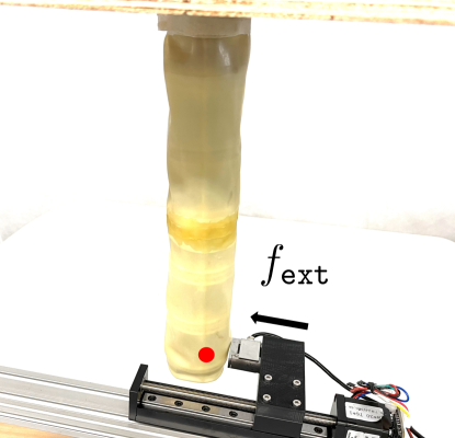
(a) Experimental setup

(b) Experimental results of transverse stiffness

Figure 5: Experiments for open-loop stiffening

We measured the stiffness values under different open-loop tendon forces $\mu>0$ in the interval $[0,45]$ N. Each experiment was repeatedly conducted three times under the same conditions in order to improve reliability. The experimental results are shown in Fig. 5(b), where “$\times$” represents the mean values of the calculated stiffness for all $\mu$, and the error bars are $\pm 1$ standard deviation. This clearly verifies the theoretical results in Proposition 1. The correlation coefficient between $\mu$ and the stiffness is 0.989, which illustrates the strong linearity – exactly coinciding with the equation (17).

VI-C Closed-loop experiments

In order to apply the proposed real-time control algorithm to the experimental platform, we first conducted the identification procedure to estimate the parameters outlined in the fourth discussing point in Section V. It relies on the fact that at any static configuration ${\bf q}$ (i.e. with ${\bf p}=0$) the identity $\nabla_{\bf q}U({\bf q})=G({\bf q}){\bf u}$ holds true, and thus $J(\theta)=0$ with the cost function

$$J(\theta,u_{1},u_{2})$$ (61)

$$\hskip 8.5359pt:=\Big{|}\alpha_{1}\sin(n\theta)+\alpha_{2}\theta-[g_{0}+g_{1}(\theta)]u_{1}+[g_{0}-g_{1}(\theta)]u_{2}\Big{|}^{2},$$

that contains all the quantities to be identified. According to the modelling procedure in Appendix, we simply parameterised $g_{0}+g_{1}(\theta)=c_{1}+c_{2}\sin(\theta)$ with two constants $\alpha_{1}>0$ and $\alpha_{2}<0$, complying with the assumptions on the input matrix. We regulated the continuum robot to different equilibria $\theta^{j}$ ($j=1,\ldots,w$ with some $w\in\mathbb{N}_{+}$) by driving the cables, and recorded the corresponding forces $(u_{1}^{j},u_{2}^{j})$.

The identification procedure boils down to solving the optimisation

$$\underset{c_{1},\alpha_{1},\alpha_{2}>0,c_{2}<0}{\arg{\mbox{min}}}~{}\sum_{j\in\{1,\ldots,w\}}J(\theta^{j},u_{1}^{j},u_{2}^{j}).$$ (62)

We ran the identification experiments to collect data at 15 equilibria points (i.e. $w=15$) and repeated for six times. Using this data set, the identified parameters were $c_{1}=1.2143,c_{2}=-2.9015,\alpha_{1}=8.6114$ and $\alpha_{2}=0.001$.

To evaluate the performance of position control, we first considered a desired configuration $\mathbf{q}_{\star}=[\theta_{\star},\ldots,\theta_{\star}]^{\top}$ with $\theta_{\star}=5$ deg for the proposed control scheme. We conducted experiments for the cases without external forces under various values of the gains $\gamma$ and $K_{\tt d}$, as shown in Figs. 7-8, respectively. The second row of these figures depicts the configuration variable at the steady-state stage during $[2,8]$ s. It is worth noting that the control inputs $u_{i}$ ($i=1,2$) are mapped to the cable length $L_{i}$, as explained in Section VI-A. In all these scenarios, the transient stages lasted for less than 1.5 seconds, and the configuration variable quickly converged to small neighborhoods of the desired angle, demonstrating the high accuracy of the proposed control approach. There were no apparent overshootings in configuration variables. Our results indicate that selecting either a sufficiently small or large $K_{\tt d}$ can negatively affect the control performance during the transient stage. On the other hand, setting a large $\gamma>0$ may lead to chattering due to measurement noise at the steady-state stage, which is well understood as the deleterious effect of high-gain design in the control literature [33].

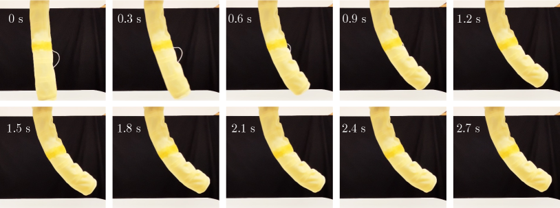
Figure 6: Photo sequence of the position control with $\theta_{\star}=10$ deg (overall bending as 60 deg) and $\gamma=1,K_{\tt d}=0.1$

(a)

(b)

(c)

(d)

(e)

(f)

(g)

(h)

(i) $K_{\tt d}=10,~{}\gamma=1$

(j) $K_{\tt d}=5,~{}\gamma=1$

(k) $K_{\tt d}=0.1,~{}\gamma=1$

(l) $K_{\tt d}=0.01,~{}\gamma=1$

Figure 7: Position control performance for the desired configuration $\theta_{\star}=5~{}{\rm deg}$ with different $K_{\tt d}$

(a)

(b)

(c)

(d)

(e)

(f)

(g)

(h)

(i) $K_{\tt d}=1,~{}\gamma=0.01$

(j) $K_{\tt d}=1,~{}\gamma=0.1$

(k) $K_{\tt d}=1,~{}\gamma=1$

(l) $K_{\tt d}=1,~{}\gamma=5$

Figure 8: Position control performance for the desired configuration $\theta_{\star}=5~{}{\rm deg}$ with different $\gamma$.

We conducted additional experiments to test the proposed control approach in different scenarios, including the desired configurations of $\theta_{\star}=10$ deg and $15$ deg, which are shown in Fig. 9. These results demonstrate that the algorithm is capable of achieving high accuracy and performance for position control. To quantify the steady performance, we study the configuration trajectories during ${\cal I}_{\tt s}:=[4,8]$ s, since for all these scenarios the system states arrive at the steady-state stage. For these two desired equilibria, the proposed design achieved high accuracy, verifying the property P1 in Proposition 4.

We summarise the accuracy achieved in these experiments with different equilibria ($5$ deg, $10$ deg and $15$ deg) and gains of $\gamma$ and $K_{\tt d}$ in Table I, where $[\theta_{\tt min},\theta_{\tt max}]$ represents the minimal and the maximal values during the interval ${\cal I}_{\tt s}$. We also give the root mean square (RMS) and the mean absolute error (MAE) for each scenario in the same table. For $\theta_{\star}=5$ deg, it achieved the highest accuracy among the three equilibria, for which the selections of $\gamma$ as $1$ and $5$ degraded the steady-state accuracy a little bit. In Fig. 6, we present a photo sequence of one of the scenarios with the desired configuration $\theta_{\star}=10$ deg, and the gains $K_{\tt d}=0.1$ and $\gamma=1$. This sequence serves as an intuitive illustration of the dynamic behaviour of the closed loop.

In addition, we report the result with a large $\gamma=10$. However, as explained in the discussion point 3) in Section V, a large $\gamma>0$ may make the desired potential energy function $U_{\tt d}$ non-convex, resulting in instability. This is consistent with the experimental results, as we observe the neutral stability with oscillating behaviours at the steady-state stage for $\gamma=10$; see Fig. 10. Evaluating the closed-loop performance in Fig. 7, we observe that a smaller gain $K_{\tt d}$ was likely to cause poor transient performance with longer time. Whereas, the experimental results in Table I show that the value of $K_{\tt d}$ within the interval $[0.1,10]$ has limited effects on the steady-state performance for position control.

(a)

(b)

(c)

(d)

(e) $\theta_{\star}=10$ deg

(f) $\theta_{\star}=15$ deg

Figure 9: Position control performance for the desired configurations $\theta_{\star}=10~{}{\rm deg}$ and $15$ deg with $K_{\tt d}=1$ and $\gamma=0.1$

TABLE I: The steady-state errors in the time interval $[4,8]$ s of different scenarios (Unit: deg)

		$K_{\tt d}=10$			$K_{\tt d}=1$			$K_{\tt d}=0.1$
$\gamma$		[$\theta_{\tt min},\theta_{\tt max}$]	RMS	MAE	[$\theta_{\tt min},\theta_{\tt max}$]	RMS	MAE	[$\theta_{\tt min},\theta_{\tt max}$]	RMS	MAE
$5$ deg	$0.01$	[4.8876, 4.9403]	4.9336	0.0664	[4.9492, 4.9532]	4.9506	0.0494	[4.9236, 4.9515]	4.9413	0.0587
	$0.1$	[4.9538, 4.9687]	4.9605	0.0395	[4.9387, 4.9556]	4.9505	0.0495	[4.9480, 4.9528]	4.9503	0.0497
	$1$	[4.9148, 4.9265]	4.9570	0.0430	[4.9148, 4.9265]	4.9219	0.0781	[4.9156, 4.9195]	4.9179	0.0821
	$5$	[4.9325, 4.9367]	4.9351	0.0649	[4.9333, 4.9425]	4.9383	0.0617	[4.9316, 4.9473]	4.9408	0.0592
$10$ deg	$0.01$	[9.5437, 10.2709]	9.8684	0.1460	[9.8328, 9.9597]	9.8824	0.1176	[9.8458, 9.9596]	9.8902	0.1098
	$0.1$	[9.8320, 9.9048]	9.8803	0.1197	[9.8328, 9.9597]	9.8810	0.1190	[9.8440, 9.9758]	9.8991	0.1009
	$1$	[9.9074, 9.9295]	9.9216	0.0784	[9.7814, 9.9044]	9.8455	0.1546	[9.8204, 9.8457]	9.8324	0.1676
	$5$	[9.8706, 9.8857]	9.8756	0.1244	[9.8955, 9.8701]	9.8884	0.1116	[9.8942, 9.8442]	9.8812	0.1188
$15$ deg	$0.01$	[12.0252, 14.9968]	14.5881	0.4266	[14.7067, 14.7753]	14.7651	0.2350	[14.7333, 14.7798]	14.7711	0.2289
	$0.1$	[14.3324, 14.9968]	14.7970	0.2044	[14.5142, 14.7350]	14.6812	0.3190	[14.7174, 17.7939]	14.7710	0.2290
	$1$	[14.6276, 14.9968]	14.8059	0.1942	[14.7499, 14.7794]	14.7632	0.2368	[14.7228, 14.7597]	14.7482	0.2519
	$5$	[14.6863, 14.7590]	14.7209	0.2792	[14.7061, 14.7307]	14.7236	0.2764	[14.7051, 14.7301]	14.7186	0.2814

Figure 10: A large $\gamma=10$ leads to unstable performance

We present experimental results demonstrating closed-loop stiffness regulation around the desired equilibria, which is related to P2 in Proposition 4. While measuring the overall stiffness is generally not manageable, we can test the transverse stiffness as outlined in Item 1) of Section V. To this end, we equipped a linear actuator perpendicularly to the tangential direction of the continuum robot at the end-effector, as shown in Fig. 3. We repeated the experiments for two different desired equilibria, namely 8 deg and 10 deg. We collected stiffness data using different gains $\gamma$ and plotted the results in Figs. 11 and 12. The results match the equation (60) in Section V that the closed-loop stiffness is affine in the control gain $\gamma$. This implied that we were able to identify the parameters $\kappa_{1}$ and $\kappa_{2}$, and use them to tune the controller for a prescribed stiffness around the desired configuration.

Finally, in order to investigate the robustness of the proposed approach, we conducted the experiments for two supplementary scenarios: one for examining the robot response in the presence of external disturbances, and the other for studying passive environmental interaction via encountering a semi-rigid foam obstruction. These setups are shown in Fig. 13, and the corresponding experimental results are presented in Fig. 14. Specifically, Fig. 14(a) provides evidence of the remarkable robustness of the proposed controller vis-à-vis external disturbances, as it effectively made the system back to its desired configuration after the vanishing of disturbances. We also note that a larger gain $\gamma>0$ yielded a shorter recovery response. In the encounter experiments, as shown in Figs. 13(b) and 14(b), a larger value of $\gamma=5$ ensured that the robot passed the foam obstruction, resulting in a recorded trajectory that was approximately monotonic over time – indicating the robot’s stiff behaviour. In contrast, using the smaller value of $\gamma=0.1$ did not yield this effect, causing the robot to exhibit some deformation when encountering the foam and displaying real-time position fluctuations in the transient stage due to its softness.

It is important to note that although various control approaches have been proposed for continuum robotics, their suitability for achieving simultaneous control of position and stiffness in underactuated robots is limited, particularly considering the variations in actuation mechanisms across different continuum robotic platforms. Given the absence of applicable control strategies in the existing literature, this study did not provide experimental comparisons to previous works. However, our objective is to lay the groundwork for future exploration and development of experimental studies in this area.

Figure 11: Stiffness regulation with the desired configuration $\theta_{\star}=$ 8 deg ($\kappa_{1}=0.0288$ and $\kappa_{2}=0.2332$)

Figure 12: Stiffness regulation with the desired configuration $\theta_{\star}=$ 10 deg ($\kappa_{1}=0.0805$ and $\kappa_{2}=0.4305$)

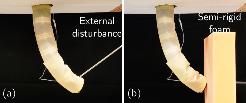
Figure 13: Experiments to evaluate the robustness of the closed-loop robotic system: (a) An external disturbance was added to the distal point of the robot; (b) The robot was controlled to encounter a semi-rigid foam obstruction.

Figure 14: Results of the robustness evaluation experiments: (Left) Applying external disturbances; (Right) Encountering a semi-rigid foam obstruction.

VII Conclusion

In this paper, we studied the modelling and control of underactuated antagonistic tendon-driven continuum robots. The proposed model possesses a configuration-dependent input matrix, which effectively captures the mechanism for open-loop stiffening through cable tension regulation. We have thoroughly analysed the assignable equilibria set and devised a potential shaping feedback controller that enables simultaneous position-and-stiffness regulation while adhering to the non-negative input constraint. To the best of the authors’ knowledge, this is the first design for such a problem. The experimental results on the robotic platform OctRobot-I demonstrate the effectiveness and reliability of the proposed approach. Our approach relies on only a few intrinsic parameters of the model, rather than depending on the complete dynamical model. This grants it remarkable robustness against modelling errors.

Along the research line, the following problems are considered as potential future works:

• As per Proposition 4, we impose the condition $\gamma<\alpha_{2}$ to guarantee the convexity of the desired potential energy function $U_{\tt d}$. It should be noted that the parameter $\alpha_{2}$ is an intrinsic characteristic of the continuum robot, and consequently the range of choices for the adaptation gain $\gamma$ is limited, which restricts our ability to control the stiffness in a relatively narrow interval. Our experimental results support this assertion. To enlarge the closed-loop stiffness range, a potential way is to make full use of jamming in the continuum robot via changing the compression level of jamming flaps [48].

• Exploring alternative desired potential energy functions may offer a promising way to enhance closed-loop performance. In addition, applying state-of-the-art energy shaping methodologies, such as those demonstrated in e.g. [50, 37], could prove valuable for solving more complex tasks for continuum robots, e.g., path following and robust simultaneous position-and-stiffness control.

• Similar to the recent works [21, 14], the approach in the paper is developed for the planar case. It is underway to extend the main results to multiple sections in a three-dimensional space. A promising way is to change the mechanical structure and actuate the overall robot in a sagittal plane for each section in order to prevent sections from twisting about their neutral axis [29]. Then, we may use the proposed approach to control sections separately in different planes, and the manipulator is capable of three-dimensional Cartesian positioning.

• Our proposed approach does not consider the actuation dynamics, opting instead to utilise a high-gain design to enforce time-scale separation and disregard these dynamics. It would be advantageous to take the actuation dynamics in to the controller synthesis by incorporating advanced robustification techniques [34].

A. Supplementary Details on Modelling

In this section, we provide additional details on the model, in particular the potential energy functions of the continuum robotic platform.

-1 Gravitational energy

In order to approximate the gravitational potential energy $U_{\tt G}$, we make the assumption that the mass is lumped at the centre of each link with the link lengths $l_{i}>0$ and the masses $m_{i}>0$ for $i\in{\cal N}$. From some basic geometric relations, we have

$$U_{\tt G}({\bf q})=\sum_{i\in{\cal N}}{l_{i}m_{i}\over 2}\left[\cos(q_{0}+\ldots+q_{i-1})-\cos(q_{0}+\ldots+q_{i})\right]$$ (63)

with the parameter $q_{0}=0$, which satisfies $U_{\tt G}(\mathbf{0}_{n})=0$.

In addition, we impose Assumption 3 about the mass and length, under which the potential energy becomes

$$U_{\tt G}({\bf q}) ~{}=~{}\alpha_{1}(1-\cos(q_{\Sigma}))$$ (64)

with

$$q_{\Sigma}~{}:=~{}\sum_{i\in{\cal N}}{\bf q}_{i},$$

and some coefficient $\alpha_{1}>0$.

-2 Elastic energy

In the designed continuum robot, each spine segment contains two pair of helical compression springs. Since we limit ourselves to the 2-dimensional case, we only consider a pair of springs as illustrated in Fig. 15, and make the assumption below.

Assumption 6

The deformable part of the continuum manipulator consists of a fixed number of segments with constant curvature and differentiable curves everywhere [14]. $\triangleleft$

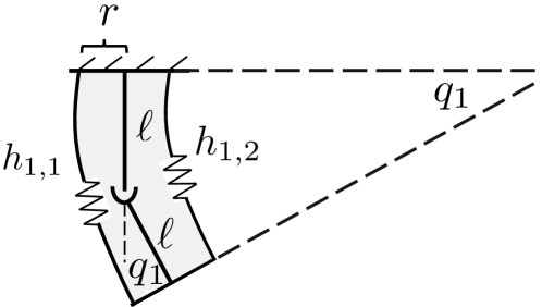
Figure 15: Illustration of the elastic potential energy in springs

In terms of the above assumptions, the boundary lengths in the $i$-th segment are given by

$$h_{i,1}=q_{i}\Big{[}\ell\cot\Big{(}{q_{i}\over 2}\Big{)}+r\Big{]},$$

$$h_{i,2}=q_{i}\Big{[}\ell\cot\Big{(}{q_{i}\over 2}\Big{)}-r\Big{]}.$$

Note that the above functions are well-posed when $q_{i}\to 0$, i.e.,

$$\lim_{q_{i}\to 0}h_{i,1}=2\ell,\quad\lim_{q_{i}\to 0}h_{i,2}=2\ell.$$

Hence, the elastic energy can be modelled as

$$U_{\tt E}=\sum_{i\in{\cal N}}{k_{i}}\left[q_{i}^{2}\Big{(}\ell^{2}\cos\Big{(}{q_{i}\over 2}\Big{)}^{2}+r^{2}\Big{)}-\ell^{2}\right]+k_{i}^{\prime}q_{i}^{2},$$ (65)

in which $k_{i}>0$ and $k_{i}^{\prime}>0$ are some elastic coefficients to characterise the elastic energies caused by the elongation and bending of springs.

In the proposed rigid-link model, each configuration variable $q_{i}$ would generally be small, i.e., $q_{i}\in[-{\pi\over 12},{\pi\over 12}]$, for which the term $\cos({q_{i}\over 2})^{2}$ takes values within $[0.983,1]$. Then, it is reasonable to make the following quadratic assumption to approximate the highly nonlinear function in (65).

Assumption 7

The elastic energy function $U_{\tt E}$ has the quadratic form

$$U_{\tt E}({\bf q})={1\over 2}{\bf q}^{\top}\Lambda{\bf q}+U_{0}$$ (66)

with a constant coefficient $U_{0}$ and a diagonalisable matrix $\Lambda:=\mbox{diag}(\alpha_{2},\ldots\alpha_{2})\succ 0$. $\triangleleft$

-3 Inertia and kinematic energy

The analytic form of the inertia matrix $M({\bf q})$ can be obtained following the standard way for rigid-link robotic models. The interested reader may find detailed procedures in [27, Chapter 8.4]. Then, the kinematic energy is given by ${1\over 2}{\bf p}M({\bf q})^{-1}{\bf p}$.

Note that the specific formulation of the inertia $M({\bf q})$ is not involved in the controller design. This makes the closed loop relatively robust, and it is unnecessary to obtain the analytic formulation of $M({\bf q})$ for experimental implementation.

-4 Input matrix

Let us use a single link to discuss the modelling of the input matrix $G({\bf q})$. We assume that the tension is uniformly distributed along the cables, and lumped forces are along the tangential directions at the middle points of the constant-curvature outline. Then, the lever’s fulcrums ${\cal L}_{1}$ and ${\cal L}_{2}$ in Fig. 2 are given by

$${\cal L}_{1}=r-{\ell\over 2}\sin(q_{i}),\quad{\cal L}_{2}=r+{\ell\over 2}\sin(q_{i}).$$

According to some basic geometric relations, we can obtain the $i$-th row of the input matrix as

$$\begin{bmatrix}G_{i,1}&G_{i,2}\end{bmatrix}=k_{u}\begin{bmatrix}r-{\ell\over 2}\sin(q_{i})&-r-{\ell\over 2}\sin(q_{i})\end{bmatrix},$$

in which $k_{u}>0$ is a coefficient to denote the loss of inputs at the virtual joint, subject to friction and viscoelastic effects [35]. Correspondingly, $g_{0}=k_{u}r$ and $g_{1}=-{1\over 2}\ell k_{u}\sin(q_{i})$. This model verifies the key assumption (8) with $\partial G_{i,j}/\partial q_{i}({\bf q})<0$.

Bowen Yi obtained his Ph.D. degree in Control Engineering from Shanghai Jiao Tong University, China in 2019. From 2017 to 2019 he was a Visiting Student at Laboratoire des Signaux et Systèmes, CNRS-CentraleSupélec, Gif-sur-Yvette, France. He has held postdoctoral positions in Australian Centre for Robotics (ACFR), The University of Sydney, NSW, Australia (2019 - 2022), and the Robotics Institute, University of Technology Sydney, NSW, Australia (Sept. 2022 - 2023). His research interests involve nonlinear systems and robotics. Dr. Yi was the recipient of the 2019 CCTA Best Student Paper Award from the IEEE Control Systems Society for his contribution on sensorless observer design.

Yeman Fan (Student Member, IEEE) received the B.E. degree in Machine Designing, Manufacturing and Automation, and the M.E. degree in Agricultural Electrification and Automation from Northwest A&F University, Yangling, China, in 2016 and 2019, respectively. He is currently pursuing the Ph.D. degree with the Robotics Institute, University of Technology Sydney, Sydney, NSW, Australia. His research interests include continuum robots and manipulators, robot control systems, and jamming technology for robotics.

Dikai Liu (Senior Member, IEEE) received the Ph.D. degree in Dynamics and Control from the Wuhan University of Technology, Wuhan, China, in 1997. He is currently a Professor in Mechanical and Mechatronic Engineering with the Robotics Institute, University of Technology Sydney, Sydney, NSW, Australia. His main research interest is robotics, including robot perception, planning and control of mobile manipulators operating in complex environments, human-robot collaboration, multi-robot coordination, and bioinspired robotics.

José Guadalupe Romero (Member, IEEE) obtained the Ph.D. degree in Control Theory from the University of Paris-Sud XI, France in 2013. Currently, he is a full time Professor at ITAM in Mexico and since July 2023 he is the Chair of the Department of Electrical and Electronic Engineering. He has over 45 papers in peer-reviewed international journals where he has also served as a reviewer. His research interests are focused on nonlinear and adaptive control, stability analysis and the state estimation problem, with application to mechanical systems, aerial vehicles, mobile robots and multi-agent systems. He currently serves as an Editor of the International Journal of Adaptive Control and Signal Processing.

References

- [1] C. Armanini, F. Boyer, A. T. Mathew, C. Duriez, and F. Renda, “Soft robots modeling: A structured overview,” IEEE Trans. Robot., vol. 39, no. 3, pp. 1728–1748, 2023.
- [2] A. Bajo and N. Simaan, “Hybrid motion/force control of multi-backbone continuum robots,” Int. J. Robot. Res., vol. 35, no. 4, pp. 422–434, 2016.
- [3] J. M. Bern, L. Z. Yañez, E. Sologuren, and D. Rus, “Contact-rich soft-rigid robots inspired by push puppets,” in Proc. IEEE Int. Conf. Soft Robot. IEEE, 2022, pp. 607–613.
- [4] C. M. Best, L. Rupert, and M. D. Killpack, “Comparing model-based control methods for simultaneous stiffness and position control of inflatable soft robots,” Int. J. Robot. Res., vol. 40, no. 1, pp. 470–493, 2021.
- [5] T. M. Bieze, F. Largilliere, A. Kruszewski, Z. Zhang, R. Merzouki, and C. Duriez, “Finite element method-based kinematics and closed-loop control of soft, continuum manipulators,” Soft Robot., vol. 5, no. 3, pp. 348–364, 2018.
- [6] D. Braganza, D. M. Dawson, I. D. Walker, and N. Nath, “A neural network controller for continuum robots,” IEEE Trans. Robot., vol. 23, no. 6, pp. 1270–1277, 2007.
- [7] T. Bretl and Z. McCarthy, “Quasi-static manipulation of a Kirchhoff elastic rod based on a geometric analysis of equilibrium configurations,” Int. J. Robot. Res., vol. 33, no. 1, pp. 48–68, 2014.
- [8] D. Bruder, X. Fu, R. B. Gillespie, C. D. Remy, and R. Vasudevan, “Data-driven control of soft robots using Koopman operator theory,” IEEE Trans. Robot., vol. 37, no. 3, pp. 948–961, 2020.
- [9] B. Caasenbrood, A. Pogromsky, and H. Nijmeijer, “Energy-shaping controllers for soft robot manipulators through port-Hamiltonian Cosserat models,” SN Comput. Sci., vol. 3, no. 6, p. 494, 2022.
- [10] H.-S. Chang, U. Halder, C.-H. Shih, N. Naughton, M. Gazzola, and P. G. Mehta, “Energy-shaping control of a muscular octopus arm moving in three dimensions,” Proc. R. Soc. A, vol. 479, no. 2270, 2023, Art. no. 20220593.
- [11] H.-S. Chang, U. Halder, C.-H. Shih, A. Tekinalp, T. Parthasarathy, E. Gribkova, G. Chowdhary, R. Gillette, M. Gazzola, and P. G. Mehta, “Energy shaping control of a CyberOctopus soft arm,” in IEEE Conf. Decis. Control. IEEE, 2020, pp. 3913–3920.
- [12] W.-H. Chen, S. Misra, Y. Gao, Y.-J. Lee, D. E. Koditschek, S. Yang, and C. R. Sung, “A programmably compliant origami mechanism for dynamically dexterous robots,” IEEE Robot. Autom. Lett., vol. 5, no. 2, pp. 2131–2137, 2020.
- [13] C. Della Santina, C. Duriez, and D. Rus, “Model-based control of soft robots: A survey of the state of the art and open challenges,” IEEE Control Syst. Mag., vol. 43, no. 3, pp. 30–65, 2023.
- [14] C. Della Santina, R. K. Katzschmann, A. Bicchi, and D. Rus, “Model-based dynamic feedback control of a planar soft robot: Trajectory tracking and interaction with the environment,” Int. J. Robot. Res., vol. 39, no. 4, pp. 490–513, 2020.
- [15] B. Deutschmann, A. Dietrich, and C. Ott, “Position control of an underactuated continuum mechanism using a reduced nonlinear model,” in Proc. IEEE Conf. Decis. Control. IEEE, 2017, pp. 5223–5230.
- [16] Y. Engel, P. Szabo, and D. Volkinshtein, “Learning to control an octopus arm with Gaussian process temporal difference methods,” in Adv. Neural. Inf. Process. Syst., vol. 18, 2005.
- [17] V. Falkenhahn, A. Hildebrandt, R. Neumann, and O. Sawodny, “Dynamic control of the bionic handling assistant,” IEEE/ASME Trans. Mechatron., vol. 22, no. 1, pp. 6–17, 2016.
- [18] F. Fan, B. Yi, D. Rye, G. Shi, and I. R. Manchester, “Learning stable Koopman embeddings,” in Proc. Amer. Control Conf., 2022, pp. 2742–2747.
- [19] Y. Fan, D. Liu, and L. Ye, “A novel continuum robot with stiffness variation capability using layer jamming: Design, modeling, and validation,” IEEE Access, vol. 10, pp. 130 253–130 263, 2022.
- [20] J. Fathi, T. J. O. Vrielink, M. S. Runciman, and G. P. Mylonas, “A deployable soft robotic arm with stiffness modulation for assistive living applications,” in Proc. IEEE Int. Conf. Robot. Autom. IEEE, 2019, pp. 1479–1485.
- [21] E. Franco and A. Garriga-Casanovas, “Energy-shaping control of soft continuum manipulators with in-plane disturbances,” Int. J. Robot. Res., vol. 40, no. 1, pp. 236–255, 2021.
- [22] B. A. Jones and I. D. Walker, “Kinematics for multisection continuum robots,” IEEE Trans. Robot., vol. 22, no. 1, pp. 43–55, 2006.
- [23] A. D. Kapadia, K. E. Fry, and I. D. Walker, “Empirical investigation of closed-loop control of extensible continuum manipulators,” in Proc. IEEE/RSJ Int. Conf. Intell. Robots Syst. IEEE, 2014, pp. 329–335.
- [24] M. Keppler, D. Lakatos, C. Ott, and A. Albu-Schäffer, “Elastic structure preserving (ESP) control for compliantly actuated robots,” IEEE Trans. Robot., vol. 34, no. 2, pp. 317–335, 2018.
- [25] H. K. Khalil, Nonlinear Systems, 3rd ed. Patience Hall, 2002.
- [26] M. J. Kim, A. Werner, F. Loeffl, and C. Ott, “Passive impedance control of robots with viscoelastic joints via inner-loop torque control,” IEEE Trans. Robot., vol. 38, no. 1, pp. 584–598, 2021.
- [27] K. M. Lynch and F. C. Park, Modern Robotics, 2nd ed. Cambridge University Press, 2019.
- [28] M. Mahvash and P. E. Dupont, “Stiffness control of surgical continuum manipulators,” IEEE Trans. Robot., vol. 27, no. 2, pp. 334–345, 2011.
- [29] A. D. Marchese and D. Rus, “Design, kinematics, and control of a soft spatial fluidic elastomer manipulator,” Int. J. Robot. Res., vol. 35, no. 7, pp. 840–869, 2016.
- [30] R. Mengacci, F. Angelini, M. G. Catalano, G. Grioli, A. Bicchi, and M. Garabini, “On the motion/stiffness decoupling property of articulated soft robots with application to model-free torque iterative learning control,” Int. J. Robot. Res., vol. 40, no. 1, pp. 348–374, 2021.
- [31] R. Ortega, M. W. Spong, F. Gómez-Estern, and G. Blankenstein, “Stabilization of a class of underactuated mechanical systems via interconnection and damping assignment,” IEEE Trans. Autom. Control, vol. 47, no. 8, pp. 1218–1233, 2002.
- [32] R. Ortega, A. van der Schaft, B. Maschke, and G. Escobar, “Interconnection and damping assignment passivity-based control of port-controlled hamiltonian systems,” Automatica, vol. 38, no. 4, pp. 585–596, 2002.
- [33] R. Ortega, A. J. Van Der Schaft, I. Mareels, and B. Maschke, “Putting energy back in control,” IEEE Control Syst. Mag., vol. 21, no. 2, pp. 18–33, 2001.
- [34] R. Ortega, B. Yi, and J. G. Romero, “Robustification of nonlinear control systems vis-à-vis actuator dynamics: An immersion and invariance approach,” Syst. Control Lett., vol. 146, 2020, Art. no. 104811.
- [35] G. Palli, G. Borghesan, and C. Melchiorri, “Modeling, identification, and control of tendon-based actuation systems,” IEEE Trans. Robot., vol. 28, no. 2, pp. 277–290, 2011.
- [36] F. Renda, M. Giorelli, M. Calisti, M. Cianchetti, and C. Laschi, “Dynamic model of a multibending soft robot arm driven by cables,” IEEE Trans. Robot., vol. 30, no. 5, pp. 1109–1122, 2014.
- [37] J. G. Romero, A. Donaire, and R. Ortega, “Robust energy shaping control of mechanical systems,” Syst. Control Lett., vol. 62, no. 9, pp. 770–780, 2013.
- [38] J. K. Salisbury, “Active stiffness control of a manipulator in Cartesian coordinates,” in Proc. IEEE Conf. Decis. Control. IEEE, 1980, pp. 95–100.
- [39] M. Takegaki and S. Arimoto, “A new feedback method for dynamic control of manipulators,” ASME J. Dyn. Syst. Meas. Control, vol. 102, pp. 119–125, 1981.
- [40] T. G. Thuruthel, Y. Ansari, E. Falotico, and C. Laschi, “Control strategies for soft robotic manipulators: A survey,” Soft Robot., vol. 5, no. 2, pp. 149–163, 2018.
- [41] T. G. Thuruthel, E. Falotico, F. Renda, and C. Laschi, “Model-based reinforcement learning for closed-loop dynamic control of soft robotic manipulators,” IEEE Trans. Robot., vol. 35, no. 1, pp. 124–134, 2018.
- [42] J. Till and D. C. Rucker, “Elastic stability of Cosserat rods and parallel continuum robots,” IEEE Trans. Robot., vol. 33, no. 3, pp. 718–733, 2017.
- [43] H. Tsukamoto, S.-J. Chung, and J.-J. E. Slotine, “Contraction theory for nonlinear stability analysis and learning-based control: A tutorial overview,” Annu. Rev. Control, vol. 52, pp. 135–169, 2021.
- [44] M. Tummers, V. Lebastard, F. Boyer, J. Troccaz, B. Rosa, and M. T. Chikhaoui, “Cosserat rod modeling of continuum robots from Newtonian and Lagrangian perspectives,” IEEE Trans. Robot., vol. 39, no. 3, pp. 2360–2378, 2023.
- [45] A. van der Schaft, -Gain and Passivity Techniques in Nonlinear Control. Springer, 2000.
- [46] J. Wang and A. Chortos, “Control strategies for soft robot systems,” Adv. Intell. Syst, vol. 4, no. 5, 2022, Art. no. 2100165.
- [47] S. Wang, R. Zhang, D. A. Haggerty, N. D. Naclerio, and E. W. Hawkes, “A dexterous tip-extending robot with variable-length shape-locking,” in Proc. IEEE Int. Conf. Robot. Autom. IEEE, 2020, pp. 9035–9041.
- [48] B. Yi, Y. Fan, and D. Liu, “A novel model for layer jamming-based continuum robots,” ArXiv Preprint, 2023, (arXiv:2309.04154).
- [49] B. Yi and I. R. Manchester, “On the equivalence of contraction and Koopman approaches for nonlinear stability and control,” IEEE Trans. Autom. Control, pp. 1–16, 2023, early access.
- [50] B. Yi, R. Ortega, D. Wu, and W. Zhang, “Orbital stabilization of nonlinear systems via mexican sombrero energy shaping and pumping-and-damping injection,” Automatica, vol. 112, 2020, Art. no. 108661.
- [51] J. Zhang, Y. Li, Z. Kan, Q. Yuan, H. Rajabi, Z. Wu, H. Peng, and W. Jianing, “A preprogrammable continuum robot inspired by elephant trunk for dexterous manipulation,” Soft Robot., vol. 10, no. 3, pp. 636–646, 2023.