Complexity of Anchored Crossing Number and Crossing Number of Almost Planar Graphs

Abstract

In this paper we deal with the problem of computing the exact crossing number of almost planar graphs and the closely related problem of computing the exact anchored crossing number of a pair of planar graphs. It was shown by [Cabello and Mohar, 2013] that both problems are NP-hard; although they required an unbounded number of high-degree vertices (in the first problem) or an unbounded number of anchors (in the second problem) to prove their result. Somehow surprisingly, only three vertices of degree greater than $3$, or only three anchors, are sufficient to maintain hardness of these problems, as we prove here. The new result also improves the previous result on hardness of joint crossing number on surfaces by [Hliněný and Salazar, 2015]. Our result is best possible in the anchored case since the anchored crossing number of a pair of planar graphs with two anchors each is trivial, and close to being best possible in the almost planar case since the crossing number is efficiently computable for almost planar graphs of maximum degree $3$ [Riskin 1996, Cabello and Mohar 2011].

1 Introduction

Determining the crossing number, i.e. the smallest possible number of pairwise transverse intersections (called crossings) of edges in a drawing in the plane, of a graph is among the most important optimization problems in topological graph theory. As such its general computational complexity is well-researched. Probably most famously, it is known that graphs with crossing number $0$, i.e. planar graphs, can be recognized in linear time [HopcroftT74, WeiKuanW99]. On the other hand, computing the crossing number of a graph in general is -hard, even in very restricted settings [GareyJ83, Hlineny06, DBLP:journals/algorithmica/PelsmajerSS11], and also -hard [Cabello13]. It is rather surprising that that problem stays hard even for almost planar graphs, which are the graphs composed of a planar graph and one more edge [DBLP:journals/siamcomp/CabelloM13].

In this paper we are particularly attracted by the last mentioned problem of computing the exact crossing number of almost planar graphs (alternatively called near-planar graphs, e.g. in [DBLP:journals/siamcomp/CabelloM13]). Closely related problems were in the focus of numerous papers including [zbMATH00881174, DBLP:journals/algorithmica/GutwengerMW05, DBLP:conf/gd/HlinenyS06, DBLP:journals/informaticaSI/Mohar06, DBLP:journals/algorithmica/CabelloM11, DBLP:journals/siamcomp/CabelloM13, DBLP:conf/compgeom/HlinenyD16]. We shall denote an almost planar graph by $G+e$ where $G$ is a planar graph and $e$ a (new) edge with both ends in $V(G)$. The problem to compute the crossing number of $G+e$ is polynomial-time solvable if $G$ is planar of maximum degree $3$, by Riskin [zbMATH00881174] and Cabello–Mohar [DBLP:journals/algorithmica/CabelloM11] – as they proved, actually, the linear-time algorithm for edge insertion by Gutwenger et al. [DBLP:journals/algorithmica/GutwengerMW05] can be used to solve it. On the other hand, the same problem to compute the crossing number of $G+e$ with planar $G$ and without restricting the degrees is -hard, as proved in Cabello and Mohar [DBLP:journals/siamcomp/CabelloM13].

1.0.1 Hardness of the anchored crossing number.

The hardness proof in [DBLP:journals/siamcomp/CabelloM13] importantly builds on the concept of anchored crossing number, which is of independent interest. The anchored crossing number $\operatorname{cr}\mbox{${}_{\!\rm a}$}(H)$ of an anchored graph $H$ is defined the same way as the ordinary crossing number, with an additional restriction that allowed drawings of $H$ (called anchored drawings) must be contained in a disk such that prescribed vertices of $H$ (the anchors) are placed (“anchored”) in prescribed distinct points on the disk boundary. See Figure 1 a). $H$ is anchored planar if the anchored crossing number is $0$ (note that a planar graph may not be anchored planar for some/all selections of the anchor vertices).

a)  b)

Figure 1: a) An example of an anchored graph. Although the graph itself is planar, its anchored crossing number equals $2$. b) Another example made of a disjoint union of two anchored planar graphs. Its anchored crossing number equals $4$.

Theorem 1.1 (Cabello and Mohar [DBLP:journals/siamcomp/CabelloM13]).

Computing the anchored crossing number of an anchored graph $H$ is -hard, even if $H$ is the union of two vertex-disjoint anchored planar graphs.

The hard instances $H$ in Theorem 1.1 have an additional property (cf. [DBLP:journals/siamcomp/CabelloM13, Corollary 2.7]), which will be important later: Each of the two disjoint anchored planar subgraphs forming $H$ has a unique anchored planar drawing (essentially), and every optimal solution to the anchored crossing number of $H$ is a union of these unique anchored planar drawings.

The hardness construction in [DBLP:journals/siamcomp/CabelloM13] had used an unbounded number of anchor vertices, but Hliněný and Salazar [DBLP:conf/isaac/HlinenyS15] noted that the conclusion of Theorem 1.1 remains true if the graph $H$ moreover has a bounded number (namely at most $16$) anchor vertices. We now discuss further details in this direction.

Let the anchored graph $H$ from Theorem 1.1 be written as a disjoint union $H=H_{1}\cup H_{2}$, where each $H_{i}$, $i=1,2$, is anchored planar with $a_{i}>0$ anchors. Observe that if $\min\{a_{1},a_{2}\}=1$, then, trivially, $H$ is anchored planar as well. If $\min\{a_{1},a_{2}\}=2=a_{1}$ (up to symmetry), then we can efficiently compute the smallest edge cut between the two anchors of $H_{1}$, and multiply it by the smallest edge cut in $H_{2}$ between the corresponding two groups (as separated by the anchors of $H_{1}$) of the anchors of $H_{2}$. This product equals, again quite trivially, the anchored crossing number of $H$. See Figure 1 b). This leaves $a_{1}=a_{2}=3$ as the simplest possibly nontrivial case of the anchored crossing number problem.

We show that the latter case is already hard in our main new result:

Theorem 1.2.

Let $H$ be an anchored graph such that $H=H_{1}\cup H_{2}$, where $H_{1}$ and $H_{2}$ are vertex-disjoint connected anchored planar graphs, each with $3$ anchors, and given alongside with anchored planar drawings $\mathcal{D}_{1}$ and $\mathcal{D}_{2}$, respectively. Moreover, assume that $H$ is such that in every optimal solution to the anchored crossing number of $H$, the subdrawing of $H_{i}$, $i\in\{1,2\}$, is equivalent (homeomorphic) up to permutations of parallel edges to the given drawing $\mathcal{D}_{i}$. Then it is -hard to compute the anchored crossing number of $H$.

Note that parallel edges do not play any essential role in the crossing-number context, since they can be subdivided to make the graph simple, or modelled by integer-weighted simple edges as we do here later from Section 2.

1.0.2 Back to the crossing number of almost planar graphs.

The special conditions on hard instances formulated in Theorem 1.2 have an interesting consequence which we informally outline next. We first recall a trick introduced in [DBLP:journals/siamcomp/CabelloM13]: Having an instance $H=H_{1}\cup H_{2}$ of the anchored crossing number problem as in Theorem 1.2, we can construct a planar graph $G_{0}:=H\cup C^{+}$ where $C^{+}$ is a (multi)cycle on the $6$ anchor vertices of $H$ in the natural cyclic order, with “sufficiently many” parallel edges between consecutive pairs of the vertices of $C^{+}$. See Figure 2. If we choose vertices $v_{i}\in V(H_{i})\setminus V(C^{+})$, $i=1,2$, then any optimal solution to the (ordinary!) crossing number of $G_{0}+v_{1}v_{2}$ leaves $C^{+}$ uncrossed, and so it is actually an anchored drawing of $G_{0}+v_{1}v_{2}$ with the anchors $V(C^{+})$.

Assuming we choose in the previous $v_{1}$ and $v_{2}$ such that the anchored crossing number of $G_{0}+v_{1}v_{2}$ equals that of $H$, we continue as follows. We modify the graph $G_{0}$ into $\bar{G}_{0}$ by blowing up every vertex of $V(H_{1})$ and every vertex of $V(H_{2})\setminus V(C^{+})$ into a “sufficiently large” cubic grid. Then every vertex of $\bar{G}_{0}$, except the three anchor vertices of $H_{2}$, is of degree at most $3$, and $\bar{G}_{0}$ is still planar (since flexibility of the anchors of $H_{2}$ allows to flip modified $H_{2}$ “inside out” within $\bar{G}_{0}$). Furthermore, the crossing number of $\bar{G}_{0}+v_{1}v_{2}$ equals the anchored crossing number of $H$. Formal details to be provided in the Appendix.

a)  b)  c)

Figure 2: An illustration to Corollary 2; how to translate the problem of the anchored crossing number (of a suitable instance as in Theorem 1.2) to that of the ordinary crossing number of an almost planar graph.  a) The depicted instance consists of a disjoint union of two (blue $P$ and red $R$) anchored planar graphs. b) Turning the previous into an almost planar instance of the ordinary crossing number problem, with a “very heavy” cycle on the former anchor vertices, a “flipped out” subdrawing of the component $R$, and an extra edge $f$ which effectively forces $P$ and $R$ to stay together inside the cycle in an optimal drawing. c) Blowing up every vertex except the 3 former red anchors into a large cubic grid (a wall), which preserves the drawing properties and stays almost planar.

Hence, in contrast to the efficiently computable case of $\operatorname{cr}(G+e)$ where $G$ is planar of maximum degree $3$ [DBLP:journals/algorithmica/CabelloM11], we prove the following (see also Figure 2): [of Theorem 1.2]* Let $G$ be a planar graph such that at most three vertices of $G$ are of degree greater than $3$, and $u,v\in V(G)$. Then it is -hard to compute the crossing number of the almost planar graph $G+uv$.

Proof.

As sketched in the main body of the paper and illustrated in Figure 2; we can take an instance $H=H_{1}\cup H_{2}$ of anchored crossing number as in Theorem 1.2, and construct a planar graph $G_{0}:=H\cup C^{+}$ where $C^{+}$ is a (multi)cycle on the $6$ anchor vertices of $H$ in the natural cyclic order, with $m$ parallel edges between consecutive pairs of the vertices of $C^{+}$. The parameter $m$ is chosen “sufficiently large”, e.g., $m\geq 2|E(H_{1})|\cdot|E(H_{2})|\geq 2\operatorname{cr}\mbox{${}_{\!\rm a}$}(H)+1$ in the worst-case scenario of $H$.

Let $e_{1}\in E(H_{1})$ and $e_{2}\in E(H_{2})$ be edges incident to anchor vertices and sharing a face in some optimal solution to the anchor crossing number $\operatorname{cr}\mbox{${}_{\!\rm a}$}(H)$, and subdivide $e_{i}$ with a new vertex $v_{i}$ for $i=1,2$. For simplicity, we use the same names $H=H_{1}\cup H_{2}$ also for the subdivided graphs. Then $\operatorname{cr}\mbox{${}_{\!\rm a}$}(H)=\operatorname{cr}\mbox{${}_{\!\rm a}$}(H+f)$ where $f=v_{1}v_{2}$. We first claim that $\operatorname{cr}(G_{0}+f)=\operatorname{cr}\mbox{${}_{\!\rm a}$}(H+f)=\operatorname{cr}\mbox{${}_{\!\rm a}$}(H)$. Indeed, $\operatorname{cr}(G_{0}+f)\leq\operatorname{cr}\mbox{${}_{\!\rm a}$}(H)$ is trivial. Assume that there is a drawing $D$ of $G_{0}+f$ with at most $\operatorname{cr}\mbox{${}_{\!\rm a}$}(H)<m/2$ crossings. Then there is an uncrossed cycle $C_{0}\subseteq C^{+}$ in $D$, and so the drawing of $C_{0}$ bounds a disk such that $D$ is an anchored drawing of $H+f$ with $\operatorname{cr}(D)\geq\operatorname{cr}\mbox{${}_{\!\rm a}$}(H)$ crossings, proving the claim.

Second, we note that there exists a fixed rotation scheme of the edges of $G_{0}$ which is defined by the given drawings $\mathcal{D}_{1}$ and $\mathcal{D}_{2}$ of Theorem 1.2, and all optimal solutions to $\operatorname{cr}\mbox{${}_{\!\rm a}$}(H+f)$ by Theorem 1.2, and hence also all optimal solutions to $\operatorname{cr}(G_{0}+f)$ by the previous paragraph, respect this rotation scheme. Furthermore, $G_{0}$ has a planar drawing which respects the same rotation scheme up to mirroring and except at the three anchor vertices $A_{1}\subseteq V(H_{1})$ (informally, the subdrawing of $H_{1}$ is “flipped out” of the multicycle $C^{+}$ in the drawing of $G_{0}$, as shown in Figure 2).

The last step of the proof is to construct a planar graph $G$ from $G_{0}$ such that all vertices of $G$ except $A_{1}\subseteq V(G)$ are of degree at most $3$, and $\operatorname{cr}(G+f)=\operatorname{cr}(G_{0}+f)$. For this we apply the technique of “cubic grids”, used for instance in [Hlineny06, DBLP:journals/algorithmica/PelsmajerSS11, Cabello13] previously. Let a cylindrical cubic grid (also called a cylindrical “wall”) of height $h$ and length $\ell$ be the following graph $H$: Start with the union of $h$ cycles of length $\ell$ each, $C_{1},\ldots,C_{h}$, such that $V(C_{i})=(v^{i}_{1},\ldots,v^{i}_{\ell})$ in this cyclic order, and add all edges $\{v^{i}_{j},v^{i+1}_{j}\}$ where $1\leq i<m$, $1\leq j\leq\ell$ and $i+j$ is odd. Then $H$ is planar and all vertices of $H$ are of degree $3$, except every second vertex of $C_{1}$ and of $C_{h}$. Let $C_{1}$ be called the outer cycle of the grid $H$.

Let $h=|E(G_{0})|^{2}$. We do the following, as illustrated in Figure 2. For every vertex $v\in V(G_{0})\setminus A_{1}$ of degree $d>3$, we take a copy $H_{v}$ of the cylindrical cubic grid of height $h$ and length $2d$, and attach every edge formerly starting in $v$ to a distinct degree-$2$ vertex of the outer cycle of $H_{v}$, in the apropriate cyclic order of the aforemtnioned rotation scheme of $G_{0}$. For the resulting graph $G$ we argue as follows. First, by the assumption on the rotation scheme of $G_{0}$, we immediately get $\operatorname{cr}(G+f)\leq\operatorname{cr}(G_{0}+f)$. Second, in any assumed optimal solution to $\operatorname{cr}(G+f)$ which has less than $\operatorname{cr}(G_{0}+f)<h/2$ crossings, and for any $v\in V(G_{0})$ replaced by $H_{v}$, one of the $h$ cycles $C_{i}\subseteq H_{v}$ is uncrossed since the crossings affect at most $2\operatorname{cr}(G+f)<h$ of these cycles. So, we may prolog every edge of $G_{0}$ attached to $H_{v}$ along a disjoint path in $H_{v}$ towards $C_{i}$, then contract uncrossed $C_{i}$ into a vertex (former $v\in V(G_{0})$) and obtain a drawing certifying $\operatorname{cr}(G_{0}+f)\leq\operatorname{cr}(G+f)$. ∎

Corollary 2 brings a natural question of whether we can efficiently compute the exact crossing number $\operatorname{cr}(G+e)$ of almost planar graphs $G+e$ where $G$ has one or two vertices of degree greater than $3$, and we discuss on this in Section 4.

Consequences of the main result are not restricted only to the crossing number almost planar graphs, but include also the following problem [DBLP:conf/isaac/HlinenyS15] of the joint crossing number in a surface: Given are two disjoint graphs $G_{1}$ and $G_{2}$, each one embedded on a fixed surface $\mathcal{S}$, and the task is to find a drawing (called simultaneous or joint) of $G_{1}\cup G_{2}$ in $\mathcal{S}$ which preserves each of the given embeddings of $G_{1}$ and $G_{2}$, and the number of crossings between $E(G_{1})$ and $E(G_{2})$ is minimized. While Hliněný and Salazar [DBLP:conf/isaac/HlinenyS15] proved that this problem is hard for the orientable surface with $6$ handles, we improve the result to: [of Theorem 1.2]* It is -hard to compute the joint crossing number of two (disjoint) graphs embedded in the triple-torus.

Proof.

We utilize the technique of face-anchors from [DBLP:conf/isaac/HlinenyS15]; for any $h\geq 1$ and the surface with $h$ handles, this technique allows us to confine prescribed $h$ vertices of the graph $H_{1}$, in the context of Theorem 1.2, to lie in prescribed $h$ faces of the graph $H_{2}$ in any optimal joint drawing of $H_{1}\cup H_{2}$. Correctness of this reduction is proved for any $h$ in [DBLP:conf/isaac/HlinenyS15, Theorem 3.1], and we simply apply it with $h=3$ onto Theorem 1.2. ∎

Lastly, we note that for all mentioned problems which are -hard, if the input includes an integer $k$, then, by standard means, it becomes -complete to decide whether a solution with at most $k$ crossings is possible.

2 Basic Definitions and Tools

In this paper we consider multigraphs by default, i.e., our graphs are allowed to have multiple edges (while loops are irrelevant here), with understanding that we can always subdivide parallel edges without changing the crossing number.

2.0.1 Drawings.

A drawing $\mathcal{G}$ of a graph $G$ in the Euclidean plane $\mathbb{R}^{2}$ is a function that maps each vertex $v\in V(G)$ to a distinct point $\mathcal{G}(v)\in\mathbb{R}^{2}$ and each edge $e=uv\in E(G)$ to a simple open curve $\mathcal{G}(e)\subset\mathbb{R}^{2}$ with the ends $\mathcal{G}(u)$ and $\mathcal{G}(v)$. We require that $\mathcal{G}(e)$ is disjoint from $\mathcal{G}(w)$ for all $w\in V(G)\setminus\{u,v\}$. In a slight abuse of notation we often identify a vertex $v$ with its image $\mathcal{G}(v)$ and an edge $e$ with $\mathcal{G}(e)$. Throughout the paper we will moreover assume that: there are finitely many points which are in an intersection of two edges, no more than two edges intersect in any single point other than a vertex, and whenever two edges intersect in a point, they do so transversally (i.e., not tangentially).

The intersection (a point) of two edges is called a crossing of these edges. A drawing $\mathcal{G}$ is planar (or a plane graph) if $\mathcal{G}$ has no crossings, and a graph is planar if it has a planar drawing. The number of crossings in a drawing $\mathcal{G}$ is denoted by $\operatorname{cr}(\mathcal{G})$. The crossing number $\operatorname{cr}(G)$ of $G$ is defined as the minimum of $\operatorname{cr}(\mathcal{G})$ over all drawings $\mathcal{G}$ of $G$.

The following is a useful artifice in crossing numbers research. In a weighted graph, each edge is assigned a positive number (the weight or thickness of the edge, usually an integer). Now the weighted crossing number is defined as the ordinary crossing number, but a crossing between edges $e_{1}$ and $e_{2}$, say of weights $t_{1}$ and $t_{2}$, contributes the product $t_{1}\cdot t_{2}$ to the weighted crossing number. For the purpose of computing the crossing number, an edge of integer weight $t$ can be equivalently replaced by a bunch of $t$ parallel edges of weights $1$; this is since we can easily redraw every edge of the bunch tightly along the “cheapest” edge of the bunch. Hence, from now on, we will use weighted edges instead of parallel edges, and shortly say crossing number to the weighted crossing number. (Note, though, that when we say a graph $G+e$ is almost planar, then we strictly mean that the added edge $e$ is of weight $1$.)

2.0.2 Anchored drawings.

Assume now a closed disk $D\subseteq\mathbb{R}^{2}$. An anchored graph [DBLP:journals/siamcomp/CabelloM13] is a pair $(H,A)$ where $A\subseteq V(H)$ is a cyclic permutation of some of its vertices; the vertices in $A$ are called the anchors of $H$. An anchored drawing of $(H,A)$ is a drawing $\mathcal{H}$ of $H$ such that $\mathcal{H}\subseteq D$ and $\mathcal{H}$ intersects the boundary of $D$ exactly in the vertices of $A$ in the prescribed cyclic order. The anchored crossing number of $(H,A)$, denoted by $\operatorname{cr}\mbox{${}_{\!\rm a}$}(H,A)$, equals the minimum of $\operatorname{cr}(\mathcal{H})$ over all anchored drawings $\mathcal{H}$ of $(H,A)$. $(H,A)$ is anchored planar if $\operatorname{cr}\mbox{${}_{\!\rm a}$}(H,A)=0$.

We shall study the following special case of an anchored graph $(H,A)$, which we call an anchored pair of planar graphs, or shortly a PP anchored graph: It is the case of $H=H_{1}\cup H_{2}$ such that $(H_{1},A_{1})$ and $(H_{2},A_{2})$ are vertex-disjoint anchored planar graphs, where $A_{i}$, $i=1,2$, is the restriction of the permutation $A$ to the anchor set of $H_{i}$.

From [DBLP:journals/siamcomp/CabelloM13] one can derive the following refined statement. In regard of weighted graphs representing parallel edges (as mentioned above), we say that a graph $G$ contains a path $P\subseteq G$ of weight $t$ if every edge of $P$ in $G$ is of weight at least $t$.

Figure 3: A high-level illustration of the assumptions on the PP anchored graph $(H,A)$ in Theorem 3; the drawing $\mathcal{D}_{1}$ of $(H_{1},A_{1})$ is sketched in red, and the drawing $\mathcal{D}_{2}$ of $(H_{2},A_{2})$ is in blue. The blue sketch emphasizes only the “heavy” path $R\subseteq H_{2}$, while the red sketch shows all paths of the family $\mathcal{Q}$. The solid red paths are all of weight $w$ and the dashed red paths are of minimum weight $w-1$ (but some edges of these paths are also of weight $w$). Note that every vertex of the graph $H_{1}$ is either a red anchor, or in the intersection of some two paths from $\mathcal{Q}$.

[extension of Theorem 1.1 [DBLP:journals/siamcomp/CabelloM13]] * Assume a PP anchored graph $(H,A)$, i.e., $H=H_{1}\cup H_{2}$ is a union of vertex-disjoint connected graphs, and denoting by $A_{i}$, $i=1,2$, the restriction of $A$ to the anchors of $H_{i}$, the graphs $(H_{1},A_{1})$ and $(H_{2},A_{2})$ are anchored planar. Let $\mathcal{D}_{i}$, $i=1,2$, be an anchored planar drawing of $(H_{i},A_{i})$. Let $w$ be any sufficiently large integer parameter, which grows polynomially in the size of $H$. Furthermore, assume the following (as informally illustrated in Figure 3):

• We have $A_{1}=(a_{1},\ldots,a_{4k})$ where $k\in\mathbb{N}$, such that there are

  • for $i=1,\ldots,k-1$, a path $Q^{1}_{i}$ in $H_{1}$ from $a_{i}$ to $a_{3k+1-i}$ of weight $w-1$, such that the edges of $Q^{1}_{i}$ incident to vertices in $A_{1}$ are of weight $w$,

  • a path $Q^{1}_{k}$ from $a_{k}$ to $a_{2k+1}$ of weight $w$, and

  • for $i=1,\ldots,k$, paths $Q^{2}_{i}$ and $Q^{3}_{i}$ in $H_{1}$ from $a_{i+k}$ to $a_{4k+1-i}$ of weight $w$.

  All paths $\mathcal{Q}=\{Q^{1}_{i},Q^{2}_{i},Q^{3}_{i}:i=1,\ldots,k\}$ are pairwise edge-disjoint, and each of the unions $\bigcup_{i\in[k]}Q^{1}_{i}$ and $\bigcup_{i\in[k]}Q^{2}_{i}\cup Q^{3}_{i}$ spans $V(H_{1})\setminus A_{1}$.

• We have $b,b^{\prime}\in A_{2}$ such that $b$ is positioned between $a_{1}$ and $a_{4k}$ within the cyclic permutation $A$, and $b^{\prime}$ is positioned between $a_{2k}$ and $a_{2k+1}$ within $A$. The graph $H_{2}$ contains a path $R\subseteq H_{2}$ of weight $w^{12}$ from $b$ to $b^{\prime}$.

• All edges of $H_{1}$, and all edges of $H_{2}$ except those of $R$, have weight at most $w^{4}$, and the edges of $R$ in $H_{2}$ have weight at most $w^{12}+w^{4}$.

• In every optimal solution to the anchored crossing number of $(H,A)$;

  • the subdrawing of $H_{i}$, $i\in\{1,2\}$, is homeomorphic to the drawing $\mathcal{D}_{i}$,

  • the path $R$ crosses the path $Q^{1}_{i}$, $1\leq i<k$, in an edge of weight $w-1$, and $R$ crosses the path $Q^{1}_{k}$ and the paths $Q^{2}_{i}$ and $Q^{3}_{i}$, $1\leq i\leq k$, in edges of weight $w$.

Then it is -hard to compute the anchored crossing number of $(H,A)$.

Proof.

       $$\begin{matrix}a_{2k+1}\\ \\ \\ \vdots\\ \\ \\ \vdots\\ \\ a_{3k}\end{matrix} \qquad a_{2k}\qquad\cdots\quad\cdots\qquad a_{k+1} \qquad a_{3k+1}\quad\cdots\quad\cdots\qquad a_{4k} \begin{matrix}a_{k}\\ \\ \vdots\\ \\ \\ \\ \vdots\\ \\ a_{1}\\ \end{matrix}$$

Figure 4: An illustration of the starting step of the proof of Theorem 3 – an example of the construction of a hard anchored crossing number instance $H_{1}\cup H_{2}$ from a SAT formula, taken from [DBLP:journals/siamcomp/CabelloM13]. Columns in the construction represent the variables of the formula, and rows represent the clauses. Here $H_{2}$ is blue, and $H_{1}$ is red (detailed alone with the anchors $A_{1}=(a_{1},\ldots,a_{4k})$ on the right). The solid thin red edges all have weight $w$ (where $w$ is a large integer) and the middle dashed red edges have weight $w-1$. For the blue solid and dashed thin edges, the weights are $w^{2}$ and $w^{2}-1$, respectively (with a slight exception of the topmost blue horizontal path), and the red and blue thick edges have weight $w^{4}$.

The reduction presented in [DBLP:journals/siamcomp/CabelloM13], as briefly sketched in Figure 4, reduces from a SAT formula $\varphi$ to a PP anchored instance $(H^{\prime},A)$ where $H^{\prime}=H^{\prime}_{1}\cup H^{\prime}_{2}$. By possibly adding dummy positive-only variables, or by duplicating clauses, we may assume that the number $k$ of variables in $\varphi$ is one more than the number of clauses in $\varphi$. Then the constructed instance satisfies all assumptions presented in Theorem 3 except those concerning the “very heavy” path $R$ in $H_{2}$, as can be straightforwardly checked in [DBLP:journals/siamcomp/CabelloM13, Section 2.1]. We thus let $H_{1}=H^{\prime}_{1}$, and suitably add a path $R$ to $H^{\prime}_{2}$ in order to produce $H_{2}$.

For the latter task, we select a suitable “diagonal” path $R_{2}$ from to lower right corner of $H^{\prime}_{2}$ (wrt. Figure 4 left) to the upper left corner, where some vertices of $R_{2}$ are subdividing some edges of $H^{\prime}_{2}$, and increase weights of all edges of $R_{2}$ by $w^{12}$. Formally, we turn $H^{\prime}_{2}$ into $H^{\prime\prime}_{2}$ by subdividing some edges as specified below, select a sequence $R_{2}$ of vertices of $H^{\prime\prime}_{2}$, and define $H_{2}:=H_{2}^{\prime\prime}\cup R$ where $R$ is a path following the vertex sequence $R_{2}$, but edge-disjoint from $H^{\prime\prime}_{2}$, and all edges of $R$ are of weight $w^{12}$. By the Jordan curve theorem, in an anchored drawing, $R$ has to intersect each of the paths $Q^{1}_{k}$ and $Q^{2}_{i},Q^{3}_{i}$ for $i=1,\ldots,k$ in an edge of weight $w$, and each of the paths $Q^{1}_{i}$ for $i=1,\ldots,k-1$ in an edge of weight at least $w-1$. This construction will hence preserve the optimality of solutions, only numerically shifted up by $+(2k+1)w^{13}+(k-1)(w-1)w^{12}$, if we can ensure by a choice of $R_{2}$ that the paths $Q^{1}_{1},\ldots,Q^{1}_{k-1}$ indeed can cross $R$ in one of their weight-$(w-1)$ edges, which we discuss in the rest of the proof.

We explain, on a high level, the basic ideas of the reduction in [DBLP:journals/siamcomp/CabelloM13]. For every choice of a variable $x_{i}$, $1\leq i\leq k$, and a clause $c_{j}$, $1\leq j\leq k-1$, of the formula $\varphi$, the blue graph $H_{2}$ contains one $3\times 3$ square subgrid $H_{2}[x_{i},c_{j}]$ (i.e., four adjacent square blue faces in the picture). Note that Figure 4 indexes the variables right to left and the clauses bottom up. Routing the red paths $Q^{2}_{i},Q^{3}_{i}$ of $x_{i}$ through the left pair of square faces of $H_{2}[x_{i},c_{j}]$ means selecting the value $x_{i}=T$. Routing the red path $Q^{1}_{j}$ of the clause $c_{j}$ through the lower pair of square faces of $H_{2}[x_{i},c_{j}]$ means that $c_{j}$ is not satisfied by any of the variables $x_{1},\ldots,x_{i}$, routing $Q^{1}_{j}$ through the upper pair of square faces of $H_{2}[x_{i},c_{j}]$ means that $c_{j}$ is satisfied by some of $x_{1},\ldots,x_{i-1}$, and “jumping up” $Q^{1}_{j}$ from lower square(s) of $H_{2}[x_{i},c_{j}]$ to upper square(s) means that $c_{j}$ is satisfied by the literal of the variable $x_{i}$. The special path $Q^{1}_{k}$ has no such options, and causes no problems.

a)
b)

Figure 5: An addition to the proof of Theorem 3; how a section of the (very heavy) blue path $R$ is inserted into the subgrid $H_{2}[x_{i},c_{i}]$.  a) For odd indices $i$, the paths $Q^{2}_{i}$ and $Q^{3}_{i}$ are routed on the left side, and there are three possibilities for the path $Q^{1}_{i}$, as depicted – in each one $R$ crosses $Q^{1}_{i}$ in a dashed edge of weight $w-1$.  b) For even indices $i$, the path $Q^{1}_{i}$ is routed at the top, and there are two possibilites for the paths $Q^{2}_{i}$ and $Q^{3}_{i}$, again as depicted – in each one $R$ again crosses $Q^{1}_{i}$ in a dashed edge of weight $w-1$.

So, there are altogether $2\cdot 3=6$ possible ways of routing the red edges across $H_{2}[x_{i},c_{j}]$ in an optimal solution, sketech above and proved in [DBLP:journals/siamcomp/CabelloM13]. Unfortunately, it is not possible to select an insertion of (a section of) $R$ in $H_{2}[x_{i},c_{j}]$ to satisfy the desired properties in each of the $6$ ways of routing simultaneously. To simply overcome this difficulty, we add a bunch of dummy all-positive variables in a bunch of dummy clauses satisfied by the first dummy variable $x_{1}$, such that, overall, $x_{1},x_{3},\ldots,x_{k^{\prime}}$ (every second) for $k^{\prime}=2k+1$ are the dummy variables set to true $T$ in an optimal solution, and that $c_{2},c_{4},\ldots,c_{k^{\prime}-1}$ are the dummy clauses which take the upper routing of their paths $Q^{1}_{j}$ across $H_{2}[x_{i},c_{j}]$ for $i>1$.

Consider the sequence $H_{2}[x_{i},c_{i}]$ of our subgrids for $i=1,2,\ldots,k^{\prime}-1$. For every $i$ odd, we know by the previous that the left routing of $Q^{2}_{i}$ and $Q^{3}_{i}$ can be taken, and for $i$ even the top routing of $Q^{1}_{i}$ can be taken, across $H_{2}[x_{i},c_{i}]$. We can thus insert the section of $R$ in $H_{2}[x_{i},c_{i}]$ as defined in Figure 5 for all $i=1,2,\ldots,k^{\prime}-1$, and then simply finish $R$ across the topmost corridor of $Q^{1}_{k^{\prime}}$ along edges of $H_{2}$, which satisfies our demand. ∎

3 Main Proof: the Hardness Reduction

Our proof of Theorem 1.2 is a bit complex, and we first informally explain what we want to achieve. In a nutshell, we are going to “embed” the gadget $(H,A)$ of Theorem 3 as an ordinary subgraph within a special “frame” PP anchored graph $F_{k}$, parameterized by the gadget size, such that $F_{k}$ forces the vertices of $A$ to be placed as expected in $(H,A)$. By the informal word “forces” we mean that any (other) drawing of $F_{k}$ violating the placement of the former anchors $A$ would require increase in the number of crossings of $F_{k}$ higher than what is the difference between the best-case and the worst-case scenarios in Theorem 3.

We adopt the following “colour coding”; the subgraph $H_{1}$ in Theorem 3 will be called red and the subgraph $H_{2}$ blue, and these colours will be correspondingly used also within the frame $F_{k}$ which will include some of the vertices and edges of $H$ (precisely, the special paths of $H$ claimed by Theorem 3(a, b)).

Figure 6: A schematic picture of the frame PP anchored graph $(F_{k},B)$ used for the reduction in Section 3 with $k=4$. The solid lines depict edges, while the dashed lines represent paths in general. The thin dashed red paths pairwise intesect in red vertices which are not (and do not need to be) explicitly specified. The red and the blue graphs are vertex-disjoint and each one has three anchors ($r_{0},r_{2},r_{4}$ of the red graph, and $b_{0},d_{1},b_{4}$ of the blue graph) and is anchored planar. The bracketed numbers represent edge weights, where $[t]$ means weight $\omega^{t}$.
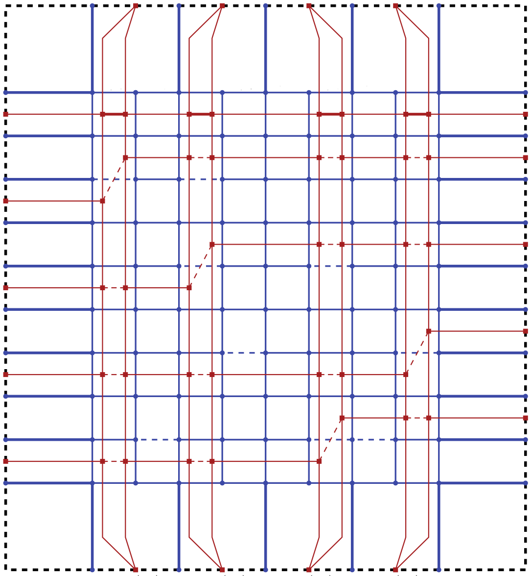
Weights of the edges emphasized with gray shade are treated specially (and a detailed picture is shown in Figure 7). The horizontal red path $P_{0}$ from $r_{0}$ to $r_{4}$ has edges of weight $\omega^{41}+\mathcal{O}(k\omega^{30})$, the horizontal blue path $P_{1}$ connecting $b_{0}$ to $b_{4}$ has, in the subpath from $b_{1}$ to $b_{3}$, edges of weight $\omega^{49}+\mathcal{O}(k\omega^{30})$, and elsewhere edges of weight $\omega^{49}+\frac{2}{5}\omega^{35}+\mathcal{O}(k\omega^{30})$; these weights are precisely specified later in the proof. The horizontal blue path $P_{2}$ connecting $c_{0}$ to $c_{4}$ has edges of weight exactly $\omega^{38}$ in the subpath from $c_{1}$ to $c_{3}$, and of weight $\omega^{38}+\frac{4}{5}\omega^{35}$ elsewhere. The vertical blue edge $b_{2}c_{2}$ is of weight exactly $\omega^{48}+2\omega^{38}-\omega^{34}$, and the vertical red edges $r_{1}r_{1}^{\prime}$ and $r_{3}r_{3}^{\prime}$ are of weight $\omega^{41}-\omega^{40}$.

Due to given space restrictions, we leave the full definition of the frame PP anchored graph $(F_{k},B)$ for the Appendix, and here we refer to a detailed sketch in Figure 6. The key feature of $(F_{k},B)$ is the use of “heavy-weight” edges, whose weight is of the form $\omega^{t}$ where $t$ is specified at each edge and $\omega$ is now seen as a variable base. Later, $\omega$ is chosen as a “sufficiently large” integer such that for every $t$, $\>\omega^{t+1}$ is always larger than the sum of a collection of crossings of weight at most $\omega^{t}$ in the reduction (with a slight abuse of traditional notation, $\omega^{t+1}>\Theta(\omega^{t})$), and that all weights are integers.

Briefly, the blue graph of $F_{k}$ has $3$ anchors $B_{2}=\{b_{0},b_{4},d_{1}\}\subseteq B$, and consists of the vertices lying on two horizontal paths $P_{1}$ from $b_{0}$ to $b_{4}$ of length $4k+4$ and $P_{2}$ from $c_{0}$ to $c_{4}$ of length $4k+2$, of four special vertices $d_{0},d_{1},d_{2},d_{4}$, and of the vertices of a vertical path $R$ from $c_{2}$ to $d_{2}$ of weight exactly $\omega^{48}$ (cf. Theorem 3(b) with $w=\omega^{4}$). Additional edges exist in $F_{k}$ between the specified blue vertices as sketched in Figure 6 and detailed in the Appendix. The red graph of $F_{k}$ has again $3$ anchors $B_{1}=\{r_{0},r_{2},r_{4}\}\subseteq B$, and consists of the vertices lying on a cycle $C_{0}$ of length $4k+3$ passing through $r_{2}$, of the vertices on a horizontal path $P_{0}$ from $r_{0}$ to $r_{4}$ of length $4k+3$, and of (the vertices of) a collection $\mathcal{Q}$ of $k+2k=3k$ edge-disjoint paths of weight $\omega^{4}-1$ or $\omega^{4}$ (as in Theorem 3(a) with $w=\omega^{4}$) which connect pairs of vertices of $P_{0}$. Again, further edges exist in $F_{k}$ between vertices of the red path $P_{0}$ and the red cycle $C_{0}$, as sketched in Figure 6 and detailed in the Appendix. Moreover, all end-edges of the paths in $\mathcal{Q}$ (i.e., those incident to $P_{0}$) are of weight $\omega^{4}$. and the second condition of Theorem 3(d) is met by the paths in $\mathcal{Q}$.

As previously sketched in Figure 6, the frame anchored graph $(F_{k},B)$ is constructed as a disjoint union $F_{k}=F_{k}^{1}\cup F_{k}^{2}$ and $B=B_{1}\cup B_{2}$, where the component $F_{k}^{1}$ is coded as red and $F_{k}^{2}$ as blue. In red $F_{k}^{1}$, we have the anchors $B_{1}=\{r_{0},r_{2},r_{4}\}$, a cycle $C_{0}$ passing through $r_{2}$, a path $P_{0}$ from $r_{0}$ to $r_{4}$, and:

• The vertices of $P_{0}$ are in order $V(P_{0})=(r_{0},r_{0}^{1},\ldots,r_{0}^{2k},r_{1},r_{3},r_{0}^{2k+1},\ldots,r_{0}^{4k},r_{4})$. The weights of its edges are $\omega^{41}+\mathcal{O}(k\omega^{30})$ and are exactly specified below in the proof. Regarding the collection of paths $\mathcal{Q}$ from Theorem 3, their ends are identified with vertices of $P_{0}$ as $a_{i}=r_{0}^{i}$ for $i=1,\ldots,4k$, and their weights are set according to Theorem 3 and $w=\omega^{4}$.

• The vertices of $C_{0}$ are in cyclic order $V(C_{0})=(r_{2},s_{0}^{1},\ldots,s_{0}^{2k},r_{1}^{\prime},r_{3}^{\prime},s_{0}^{2k+1},\ldots,$ $s_{0}^{4k},r_{2})$. The edges of $C_{0}$ are all of weight $\omega^{49}$, and there are additional two edges $r_{1}^{\prime}r_{1}$ and $r_{3}^{\prime}r_{3}$ of weight $\omega^{41}-\omega^{40}$ and $4k$ edges $r_{0}^{i}s_{0}^{i}$ of weight $\omega^{30}$ for $i=1,\ldots,4k$.

In blue $F_{k}^{2}$, we have the anchors $B_{2}=\{b_{0},d_{1},b_{4}\}$, a path $P_{1}$ from $b_{0}$ to $b_{4}$, a path $P_{2}$ from $c_{0}$ to $c_{4}$, a path $R$ from $c_{2}$ to $d_{2}$, three vertices $d_{0},d_{1},d_{4}$, and:

• The vertices of $P_{1}$ are in order $V(P_{1})=(b_{0},b_{0}^{1},\ldots,b_{0}^{k},b_{1},b_{0}^{k+1},\ldots,b_{0}^{2k},b_{2},b_{0}^{2k+1},\ldots,b_{0}^{3k},b_{3},$ $b_{0}^{3k+1},\ldots,b_{0}^{4k},b_{4})$. The vertices of $P_{2}$ are in order $V(P_{2})=(c_{0}=c_{0}^{1},\ldots,c_{0}^{k},c_{1},c_{0}^{k+1},\ldots,c_{0}^{2k},c_{2},$ $c_{0}^{2k+1},\ldots,c_{0}^{3k},c_{3},c_{0}^{3k+1},\ldots,c_{0}^{4k}=c_{4})$. The edges of $P_{1}$ are of weight $\omega^{49}+\mathcal{O}(k\omega^{30})$ between $b_{1}$ and $b_{3}$ and of weight $\omega^{49}+\mathcal{O}(k\omega^{34})+\mathcal{O}(k\omega^{30})$ elsewhere, and are exactly specified below in the proof. The edges of $P_{2}$ are of weight $\omega^{38}$ between $c_{1}$ and $c_{3}$ and $\omega^{38}+\frac{4}{5}\omega^{35}$ elsewhere.

• There is an edge $b_{2}c_{2}$ of weight $\omega^{48}+2\omega^{38}-\omega^{34}$, two edges $b_{1}c_{1}$ and $b_{3}c_{3}$ of weight $\omega^{35}$, and $4k$ edges $b_{0}^{i}c_{0}^{i}$ of weight $\omega^{30}$ for $i=1,\ldots,4k$.

• There is a path $R$, as specified in Theorem 3(b), from $c_{2}$ to $d_{2}$ of weight $\omega^{48}$. There are $7$ additional edges $c_{0}d_{0}$, $d_{0}d_{1}$, $d_{0}d_{2}$, $d_{1}d_{4}$, $d_{2}d_{4}$, $d_{4}c_{4}$, each of weight $\omega^{49}$.

One can easily check from Figure 6 that each of $(F_{k}^{1},B_{1})$ and $(F_{k}^{2},B_{2})$ is anchored planar.

Note that we do not require to exactly specify the paths of $\mathcal{Q}$, in particular they share their internal vertices in an unspecified way, but we do require the properties stated in Theorem 3 to hold for them. With respect to the drawing in Figure 6, we call the gadget region of $(F_{k},B)$ the region bounded by the blue horizontal path from $c_{0}$ to $c_{4}$ and the path $(c_{0},d_{0},d_{2},d_{4},c_{4})$. We have the following claim.

* The anchored crossing number of the PP anchored graph $(F_{k},B)$ defined above, for $k\geq 2$ and any sufficiently large $\omega$ (divisible by $5(5k+7)$), equals

$$\operatorname{cr}\mbox{${}_{\!\rm a}$}(F_{k},B)=\gamma(k):= 2\omega^{90}-\omega^{89}+(4k+2)\omega^{79}+2\omega^{76}-\omega^{75}+4k\omega^{71}$$

$$+ c_{1}(k)\omega^{65}+c_{2}(k)\omega^{60}+3k\omega^{52}-k\omega^{48}+6k\omega^{42}+\frac{12}{5}k\omega^{39},$$

where $c_{1}(k)=\frac{2}{5(5k+7)}(30k^{2}+58k+20)$ and $c_{2}(k)=\frac{2}{3(5k+7)}(16k^{3}+39k^{2}+20k)$.

Any anchored drawing of $(F_{k},B)$ with at most $\gamma^{+}(k):=\gamma(k)+\omega^{34}-\omega^{30}-1$ crossings is homeomorphic, with a possible exception of the paths of $\mathcal{Q}$, to that in Figure 6, and the internal vertices of all paths of $\mathcal{Q}$ are drawn in the gadget region and their edges cross the path $P_{2}$ from $c_{0}$ to $c_{4}$ and $R$ as depicted.

Figure 7: A detail of the “ordering” of vertices on the paths $P_{0}$ and $P_{1}$ of the frame $F_{k}$ from Figure 6, where $k=4$. Only the half to the right of $b_{2}c_{2}$ is shown, and the other half is symmetric. The edges of $P_{0}$, going from $r_{1}$ on the left to $r_{4}$ on the right, have weights $\omega^{41}+\frac{i(i+1)}{5k+7}\omega^{30}$ for $i=0,1,\ldots,2k+1$. The edges of $P_{1}$, going from $b_{2}$ on the left to $b_{4}$ on the right, have weights $\omega^{49}+\frac{i(i+2)}{5k+7}\omega^{30}$ for $i=0,1,\ldots,k$ and $\omega^{49}+\frac{2}{5}\omega^{35}+\frac{i(i+2)}{5k+7}\omega^{30}$ for $i=k+1,\ldots,2k+1$. Using straightforward calculus, one can compute that “sliding” vertices of $P_{0}$ across the vertical edge $b_{3}c_{3}$ (in any direction) would increase the weight of crossings by $\geq\frac{1}{5(5k+7)}\omega^{65}$, and “sliding” with respect to other depicted vertical blue edges would increase the weight by $\geq\frac{1}{5k+7}\omega^{60}$.

We organize arguments leading to each term of the formula for $\gamma(k)$ stepwise from higher to lower order terms of edge weights.

1. The blue path $P_{1}$ of weight $\geq\!\omega^{49}$ must not cross the red path $P_{0}$ of weight $\geq\!\omega^{41}$ since that would result in crossings of weight at least $2\omega^{90}>\gamma^{+}(k)$, and likewise with $P_{1}$ and $C_{0}$. So, by the Jordan curve theorem, the two red edges $r_{1}r_{1}^{\prime}$ and $r_{3}r_{3}^{\prime}$ of weight $\omega^{41}-\omega^{40}$ must cross $P_{1}$, contributing crossing weight at least $2\omega^{90}-2\omega^{89}$. The $4k$ red edges of weight $\omega^{30}$ from $P_{0}$ to $C_{0}$ similarly make $4k\omega^{79}$ crossings with $P_{1}$. Further, there are edge-disjoint paths from $b_{2}$ to $d_{1}$ of combined weight $\omega^{48}+2\omega^{38}$; these are formed by the path $b_{2}c_{2}+R$ of weight $\omega^{48}$, by a path from $b_{2}$ through $c_{2}$, $c_{0}$ and $d_{0}$ of weight $\omega^{38}$, by a path from $b_{2}$ through $c_{2}$, $c_{4}$ and $d_{4}$ of weight $\omega^{38}-\omega^{34}$, and by a path from $b_{2}$ through $b_{3}$, $c_{3}$ and $c_{4}$ of weight $\omega^{34}$. These contribute weight $\omega^{89}+2\omega^{79}$ of crossings with $P_{0}$. Summing up, we have so far accounted for at least $2\omega^{90}-\omega^{89}+(4k+2)\omega^{79}>\gamma(k)-2\omega^{76}+\omega^{75}$ enforced crossings.

2. The next step is to prove that $P_{2}$ is drawn disjoint from $P_{0}$ and drawn above it, and all $c_{1}b_{1}$, $c_{2}b_{2}$, $c_{3}b_{3}$ cross $P_{0}$. If, for instance, $P_{0}$ was crossed by both $b_{1}c_{1}$ and $b_{3}c_{3}$, but not by $b_{2}c_{2}$, the lower bound from (1) would rise (thanks to full weight of $b_{1}c_{1}$ and $b_{3}c_{3}$) to $2\omega^{90}-\omega^{89}+(4k+2)\omega^{79}+2\omega^{76}\geq\gamma(k)+\omega^{75}-\omega^{72}>\gamma^{+}(k)$, which is impossible. If neither of $b_{1}c_{1}$, $b_{3}c_{3}$ crosses $P_{0}$, then we (briefly) get subpaths of $P_{1}$ and $P_{2}$ of combined weight $2\frac{2}{5}\omega^{35}+2\frac{4}{5}\omega^{35}=(2+\frac{2}{5})\omega^{35}$ which cross the path $P_{0}$ or edges $r_{1}r_{1}^{\prime}$, $r_{3}r_{3}^{\prime}$, and this contributes an additional weight $(2+\frac{2}{5})(\omega^{76}-\omega^{75})$ of crossings, again exceeding $\gamma^{+}(k)$. We leave remaining details and subcases for the Appendix.

3. Using (2), we may count crossings of $P_{0}$ with the edges $c_{1}b_{1}$, $c_{2}b_{2}$, $c_{3}b_{3}$ and the $4k$ blue edges of weight $\omega^{30}$ between $P_{1}$ and $P_{2}$. At this point, our lower bound gets to $2\omega^{90}-\omega^{89}+(4k+2)\omega^{79}+2\omega^{76}-\omega^{75}+4k\omega^{71}>\gamma^{+}(k)-\omega^{66}$.

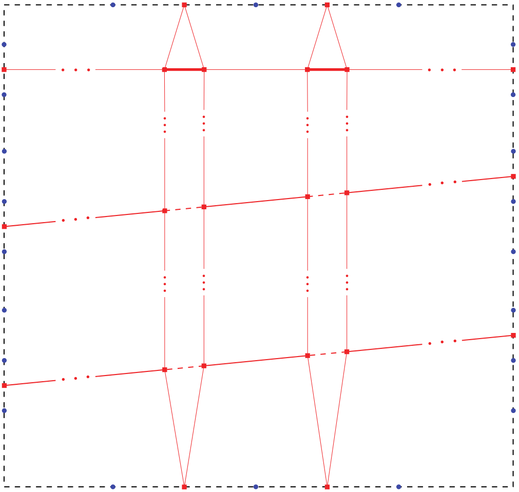
4. Next comes the crucial step of the reduction – at cost of additional $c_{1}(k)\omega^{65}+c_{2}(k)\omega^{60}$ weight of crossings, we “order” the vertical blue edges which stretch between the paths $P_{1}$ and $P_{2}$ as alternating with the internal vertices of the red path $P_{0}$. This rather long technical step is detailed in the Appendix, and here we only outline its core idea which is based on simple calculus as follows. Consider an arbitrary quadratic polynomial $p(x)$ which is increasing on $\mathbb{R}^{+}$. Then, for any $a>0$, the minimum of the function $p(x)+p(y)$ conditioned by $x+y=a$ is attained at $x=y$, that is when $x=a/2$. A slight adjustment (suitable for integer values of $x$) of this idea is used to determine fine weights of the edges of the paths $P_{0}$ and $P_{1}$ where, essentially, $x$ means the index of an edge of $P_{0}$ and $y$ that of an edge of $P_{1}$. Such fine weights then enforce precise mutual positions of the edges of $P_{0}$ and $P_{1}$, and in turn the desired alternating ordering of the vertical red and blue edges incident to $P_{0}$ and $P_{1}$. A closer idea of this principle can be obtained by looking at an example of concrete edge weights in Figure 7.

5. Points (1)–(4) together imply that the weight of crossings in $(F_{k},B)$ is at least $\gamma(k)-3k\omega^{52}$. So, none of the paths of $\mathcal{Q}$ may cross $P_{1}$ since that would add $\omega^{49+4}=\omega^{53}$. Then each of the paths of $\mathcal{Q}$ crosses the blue edge $c_{2}b_{2}$ of weight $\omega^{48}+2\omega^{38}-\omega^{34}$, or the path $R$ plus two sections of the path $P_{2}$ of combined weight $\omega^{48}+2\omega^{38}$. Since $2k$ of the paths of $\mathcal{Q}$ are of weight $\omega^{4}$ and $k$ of them of weight $\omega^{4}-1$, by Theorem 3(a), we have at least $(\omega^{48}+2\omega^{38}-\omega^{34})(3k\omega^{4}-k)\geq 3k\omega^{52}-k\omega^{48}+6k\omega^{42}-5k\omega^{38}$ more crossings from that. Moreover, each of the paths of $\mathcal{Q}$ crosses sections of $P_{2}$ between $c_{0}$–$c_{1}$ and $c_{3}$–$c_{4}$ of weight $\frac{4}{5}\omega^{35}$ (plus the edges $b_{1}c_{1}$ and $b_{3}c_{3}$), contributing another $\frac{4}{5}\omega^{35}(3k\omega^{4}-k)=\frac{12}{5}k\omega^{39}-\frac{4}{5}k\omega^{35}$. All these together raise the lower bound to at least $\gamma(k)-5k\omega^{38}-\frac{4}{5}k\omega^{35}\geq\gamma^{+}(k)-(5k+1)\omega^{38}$.

6. Assume that some of the internal vertices of a path in $\mathcal{Q}$ lie outside of the gadget region (informally, below $P_{2}$). That would force an additional crossing between such a path and $c_{1}b_{1}$ or $c_{3}b_{3}$ of weight $\geq\!(1-\frac{4}{5})\omega^{35+4}$ (or with e.g. $P_{2}$ of even higher weight), exceeding $\gamma^{+}(k)$. Therefore, despite the paths of $\mathcal{Q}$ may cross $R$ of weight $\omega^{48}$ with their minimum weight $\omega^{4}-1$ or $\omega^{4}$, since all internal vertices of all paths of $\mathcal{Q}$ lie in the gadget region, their crossings with $P_{2}$ of weight $\omega^{38}$ are always on the end-edges which are of weight $\omega^{4}$ by Theorem 3(a). This improves the estimate on the crossings carried by the paths of $\mathcal{Q}$ from (5) to $\geq\omega^{48}(3k\omega^{4}-k)+(2\omega^{38}+\frac{4}{5}\omega^{35})\cdot 3k\omega^{4}=3k\omega^{52}-k\omega^{48}+6k\omega^{42}+\frac{12}{5}k\omega^{39}$, which raises our lower bound to the desired $\gamma(k)$.

A drawing with $\gamma(k)$ crossings is as in Figure 6 with details as in Figure 7. Hence, we have finished a proof of $\operatorname{cr}\mbox{${}_{\!\rm a}$}(F_{k},B)=\gamma(k)$. Furthermore, if any of the assumptions of the previous analysis was violated, the crossing number would exceed $\gamma^{+}(k)$, and any one additional crossing not sketched in Figure 6 and not being only between paths of $\mathcal{Q}$ would add weight of at least $\omega^{30+4}-\omega^{30}$, and again $\gamma(k)+\omega^{34}-\omega^{30}>\gamma^{+}(k)$, which confirms the rest of Lemma 3.

Proof.

The arguments sketched in the main paper body actually present a full proof of Lemma 3 except for the technical steps (2) and (4). We hence do not repeat the other arguments, but only give details of these two steps

Regarding (2), once we prove that all three $c_{1}b_{1}$, $c_{2}b_{2}$, $c_{3}b_{3}$ cross $P_{0}$, we raise the lower bound from (1) to at least $2\omega^{90}-\omega^{89}+(4k+2)\omega^{79}+2\omega^{76}-\omega^{75}>\gamma^{+}(k)-\omega^{72}$, and hence $P_{2}$ could not cross $P_{0}$ and had to be above it. It thus suffices to analyze all possibilities that some of $c_{1}b_{1}$, $c_{2}b_{2}$, $c_{3}b_{3}$ do not cross $P_{0}$.

1. Neither of $c_{1}b_{1}$, $c_{3}b_{3}$ cross $P_{0}$. Then (regardless of $c_{2}b_{2}$) the weight of crossings of order $\omega^{76}$ sums to at least $2\cdot\frac{4}{5}\omega^{76}$ between $P_{0}$ and $P_{2}$, precisely, with the sections of $P_{2}$ between $c_{0}$–$c_{1}$ and $c_{3}$–$c_{4}$. In addition to that, we have a subpath from $b_{0}$ to $b_{4}$, using the edges $b_{1}c_{1}$, $b_{3}c_{3}$ and the section of $P_{2}$ between $c_{1}$–$c_{3}$, of weight $\frac{2}{5}\omega^{35}$. This subpath must cross twice $P_{0}\cup\{b_{1}c_{1},b_{3}c_{3}\}$ and, importantly, the possible crossing(s) with $P_{0}$ is in addition to the crossings between $P_{0}$ and $P_{2}$ counted in (1) if $b_{2}c_{2}$ does not cross $P_{0}$. So, this adds (neglecting the lower-order terms) $2\cdot\frac{2}{5}\omega^{76}$ more crossings between $P_{0}$ and $P_{2}$. Altogether, with the lower bound of (1), we get at least $2\omega^{90}-\omega^{89}+(4k+2)\omega^{79}+\frac{12}{5}\omega^{76}-\omega^{75}>\gamma^{+}(k)$ crossings, which is impossible.

2. Exactly one of $c_{1}b_{1}$, $c_{3}b_{3}$ crosses $P_{0}$. Here we reuse “one half” of the argument in (i.) plus the weight of the crossing of one of $c_{1}b_{1}$, $c_{3}b_{3}$ with $P_{0}$ to derive an analogous contradiction.

3. Both of $c_{1}b_{1}$, $c_{3}b_{3}$ cross $P_{0}$, but $b_{2}c_{2}$ does not. Then the lower bound from the arguments of (1) can be slightly improved, since the path $R$ and twice the path $P_{2}$ cross $P_{0}$, and in addition to that, we count the crossings of $c_{1}b_{1}$ and $c_{3}b_{3}$ with $P_{0}$. So, we improve it to at least $2\omega^{90}-\omega^{89}+(4k+2)\omega^{79}+2\omega^{76}>\gamma(k)+\omega^{75}-\omega^{72}>\gamma^{+}(k)$, which is again impossible.

Regarding (4), we first note that the graph $(F_{k},B)$ is symmetric along the vertical axis, except the paths of $\mathcal{Q}$. Since the paths of $\mathcal{Q}$ are handled only after our point, we can now assume full symmetry and prove the claim only for the right-hand side of $(F_{k},B)$, as depicted in Figure 7, and then multiply the crossings by $2$.

We recapitulate where we stand with our drawing of $(F_{k},B)$ after (1)–(3). We have got pairwise noncrossing cycle $C_{0}$ and paths $P_{1}$, $P_{0}$ and $P_{2}$ drawn in this order bottom up (Figure 6). All crossings of weight of order $\omega^{66}$ and higher have already been counted to equality with $\gamma(k)$. There are two edges of weight $\omega^{41}-\omega^{40}$ between $C_{0}$ and $P_{0}$ crossing $P_{1}$, and $4k$ such edges of weight $\omega^{30}$. There is an edge of weight $\omega^{48}+2\omega^{38}-\omega^{34}$ and two edges of weight $\omega^{35}$ between $P_{1}$ and $P_{2}$ crossing $P_{0}$, and again $4k$ such edges of weight $\omega^{30}$. Besides the already counted weights, these listed edges contribute crossings of weights of order only $\omega^{65}$ and $\omega^{60}$ (including their possible mutual crossings).

Our proof strategy is the following; we will show a concrete drawing, called the normal drawing, in which the above described crossings contribute exactly as expected in the formula for $\gamma(k)$ in the part $c_{1}(k)\omega^{65}+c_{2}(k)\omega^{60}$ (the drawing in Figure 7), and then we will argue that in any drawing in which the above listed edges (the vertical blue and red ones of weights $\omega^{35}$and $\omega^{30}$) are not as in our normal drawing, we can decrease the total crossing number by $\Omega(\omega^{60})$. This possible drop in the crossing number in turn certifies that the arbitrary considered drawing would exceed $\gamma^{+}(k)$ crossings, and hence is impossible in our claim. In this setup of a proof, it also comes for free that all crossings potentially occuring in $(F_{k},B)$, which are not counted prior to this point and are not among the crossings listed above, are of weight of order strictly less than $\omega^{60}$.

The weights of the edges of $P_{0}$ and $P_{1}$ are precisely as follows (Figure 7):

1. For $P_{0}$, $V(P_{0})=(r_{0},r_{0}^{1},\ldots,r_{0}^{2k},r_{1},r_{3},r_{0}^{2k+1},\ldots,r_{0}^{4k},r_{4})$, the weight of $r_{1}r_{3}$ is exactly $\omega^{41}$, the weight of $r_{0}^{2k}r_{1}$ and of $r_{3}r_{0}^{2k+1}$ is $\omega^{41}\!+\frac{2}{5k+7}\omega^{30}$, the weight of $r_{0}^{2k+i-1}r_{0}^{2k+i}$ and of $r_{0}^{2k-i+1}r_{0}^{2k-i}$ is $\omega^{41}\!+\frac{i(i+1)}{5k+7}\omega^{30}$ for $i=2,\ldots,2k$, and the weight of $r_{0}r_{0}^{1}$ and of $r_{0}^{4k}r_{4}$ is $\omega^{41}\!+\frac{(2k+1)(2k+2)}{5k+7}\omega^{30}$.

2. For $P_{1}$, $V(P_{1})=(b_{0},b_{0}^{1},\ldots,b_{0}^{k},b_{1},b_{0}^{k+1},\ldots,b_{0}^{2k},b_{2},b_{0}^{2k+1},\ldots,b_{0}^{3k},b_{3},b_{0}^{3k+1},$ $\ldots,b_{0}^{4k},b_{4})$, we resort to describing the weights only from $b_{2}$ till $b_{4}$. The weight of $b_{2}b_{0}^{2k+1}$ is exactly $\omega^{49}$, the weight of $b_{0}^{2k+i}b_{0}^{2k+i+1}$ is $\omega^{49}\!+\frac{i(i+2)}{5k+7}\omega^{30}$ for $i=1,\ldots,k-1$, the weight of $b_{0}^{3k}b_{3}$ is $\omega^{49}\!+\frac{k(k+2)}{5k+7}\omega^{30}$, the weight of $b_{3}b_{0}^{3k+1}$ is $\omega^{49}\!+\frac{2}{5}\omega^{35}\!+\frac{(k+1)(k+3)}{5k+7}\omega^{30}$, the weight of $b_{0}^{3k+i}b_{0}^{3k+i+1}$ is $\omega^{49}\!+\frac{2}{5}\omega^{35}\!+\frac{(i+k+1)(i+k+3)}{5k+7}\omega^{30}$ for $i=1,\ldots,k-1$, and the weight of $b_{0}^{4k}b_{4}$ is $\omega^{49}\!+\frac{2}{5}\omega^{35}\!+\frac{(2k+1)(2k+3)}{5k+7}\omega^{30}$.

We count the crossings in a normal drawing as in Figure 7:

• Concerning total crossings of weight of order $\omega^{65}$, we have $2k$ red edges of weight $\omega^{30}$ crossing the sections of $P_{1}$ between $b_{0}$–$b_{1}$ and $b_{3}$–$b_{4}$, and two blue edges of weight $\omega^{35}$ crossing $P_{0}$ in edges of weight $\frac{(k+1)(k+2)}{5k+7}$. In total

  $$2k\omega^{30}\cdot \frac{2}{5}\omega^{35}+2\omega^{35}\cdot\frac{(k+1)(k+2)}{5k+7}\omega^{30}=\frac{2}{5(5k+7)}(30k^{2}+58k+20)\omega^{65}$$

  $$=c_{1}(k)\omega^{65}.$$

• Concerning total crossings of weight of order $\omega^{60}$, and considering only the right-hand side as in Figure 7, we get crossings of $2k$ red edges of weight $\omega^{30}$ with the edges of $P_{1}$ from $b_{0}^{2k+1}$ to $b_{0}^{4k}$, and crossings of $2k$ blue edges of weight $\omega^{30}$ with the edges of $P_{0}$ from $r_{3}$ to $r_{4}$ except with the edge of weight $\frac{(k+1)(k+2)}{5k+7}$ (counted in the previous point). These sum to

  $$\omega^{30}\cdot \sum_{i=1}^{2k}\frac{i(i+2)}{5k+7}\omega^{30}+\omega^{30}\cdot\left[\,\sum_{i=1}^{2k+1}\frac{i(i+1)}{5k+7}-\frac{(k+1)(k+2)}{5k+7}\right]\omega^{30}$$

  $$=\frac{1}{3(5k+7)}(16k^{3}+39k^{2}+20k),$$

  which multiplied by $2$ gives $c_{2}(k)$.

Now, we handle an arbitrary drawing of $(F_{k},B)$ which conforms to the bounds shown in (1)–(3), but is not our normal drawing described by Figure 7. As argued above, it is enough for this purpose to consider only edges depicted in Figure 7, and know that the depicted vertical edges indeed cross the horizontal paths $P_{1}$ and $P_{2}$ somewhere. Crossings of weight of order strictly higher than $\omega^{65}$ are not relevant in this analysis (as they are enforced and have been counted, and so new such ones cannot even arise), and crossings of weight of order strictly less than $\omega^{60}$ can be ignored at this stage (by the choice of sufficiently large $\omega$).

We denote by $t^{0}_{i}=\frac{i(i+1)}{5k+7}$ and $t^{1}_{i}=\frac{i(i+2)}{5k+7}$, and refer to Figure 7. The $i$-th edge of the red path $P_{0}$, counted from $r_{3}$ towards $r_{4}$, is of weight $\omega^{41}\!+t^{0}_{i}\omega^{30}$, and the $(i+1)$-th edge of the blue path $P_{1}$, counted from $b_{2}$ towards $b_{4}$, is of weight $\omega^{49}\!+t^{1}_{i}\omega^{30}$, resp. of weight $\omega^{49}\!+\frac{2}{5}\omega^{35}\!+t^{1}_{i}\omega^{30}$ if $i>k$. We also denote the vertical red edges (of weight $\omega^{30}$) incident to the path $P_{0}$ by $f^{0}_{1},\ldots,f^{0}_{2k}$ such that $f^{0}_{i}$ is incident to the vertex $r_{0}^{2k+i}$, and the vertical blue edges (of weight again $\omega^{30}$) incident to the path $P_{1}$ by $f^{1}_{1},\ldots,f^{1}_{2k+1}$ such that $f^{1}_{i}$ is incident to the vertex $b_{0}^{2k+i}$ for $i\leq k$,  $f^{1}_{k+1}$ is incident to $b_{3}$, and $f^{1}_{i}$ is incident to $b_{0}^{2k+i-1}$ for $i\geq k+2$.

One can easily check that in our normal drawing, we have, naturally, $f^{0}_{i}$ crossing $P_{1}$ in the edge of weight coefficient $t^{1}_{i}$,  $f^{1}_{j}$ crossing $P_{0}$ in the edge of weight coefficient $t^{0}_{j}$, and no $f^{0}_{i}$ is crossing any $f^{1}_{j}$. Assume that the drawing of $f^{0}_{i}$ violates some of the previous conditions.

1. Assume that $f^{0}_{i}$ crosses $f^{1}_{j}$ for some $j\leq i$, and that $i-j$ is minimized with respect to that. The minimality assumption implies that $f^{1}_{j}$ crosses $P_{0}$ in the edge of $t^{0}_{i-1}$. We may “slide” the vertex $r_{0}^{2k+i}$ along the drawing of $P_{0}$ towards $r_{0}^{2k+i-1}$, such that the crossing of $f^{1}_{j}$ with $P_{0}$ changes to the edge of weight coefficient $t^{0}_{i}$. This increases the crossing weight on $P_{0}$ by $(t^{0}_{i}-t^{0}_{i-1})\omega^{30+30}\leq\frac{4k}{5k+7}\omega^{60}<(1-\frac{1}{5})\omega^{60}$ (resp., the same expression with $\omega^{65}$ if $f^{1}_{j}=b_{3}c_{3}$). On the other hand, this move saves $\omega^{60}$ (resp., $\omega^{65}$) weight of crossing between $f^{0}_{i}$ and $f^{1}_{j}$, hence decreasing the total number of crossings by at least $\frac{1}{5}\omega^{60}$.

2. A case that $f^{0}_{i}$ crosses $f^{1}_{j}$ for some $j>i$ is solved analogously, with “sliding” the vertex $r_{0}^{2k+i}$ along $P_{0}$ towards $r_{0}^{2k+i+1}$.

3. For the rest, we consider that no $f^{0}_{i^{\prime}}$ is crossing any $f^{1}_{j}$. Assume that $f^{0}_{i}$ crosses $P_{1}$ in the edge of weight coefficient $t^{1}_{j}$ for $j<i$, and that $i-j$ is maximized with respect to that. Further assume that $f^{1}_{j}\not=b_{3}c_{3}$. The maximality assumption, together with $f^{1}_{j}$ not crossing any $f^{0}_{i^{\prime}}$, imply that $f^{1}_{j}$ crosses $P_{0}$ in the edge of $t^{0}_{i+1}$. We now simultaneously “slide” the end of $f^{0}_{i}$ along the drawing of $P_{0}$ to the right and the end of $f^{1}_{j}$ along the drawing of $P_{1}$ to the left, such that $f^{0}_{i}$ and $f^{1}_{j}$ (informally) exchange positions.

   On the path $P_{1}$, we gain crossings of weight $(t^{1}_{j+1}-t^{1}_{j})\omega^{30+30}=\frac{2j+3}{5k+7}\omega^{60}$. On the path $P_{0}$, we save crossings of weight $(t^{0}_{i+1}-t^{0}_{i})\omega^{30+30}=\frac{2i+2}{5k+7}\omega^{60}$. And since $i\geq j+1$, we decrease the total crossings by at least $\frac{1}{5k+7}\omega^{60}$.

4. Under the same initial assumption as in (iii.), we consider the subcase that $f^{1}_{j}=b_{3}c_{3}$. Then the same modification of the drawing causes the following. On the path $P_{1}$, we gain crossings of weight $\frac{2}{5}\omega^{35+30}$, neglecting the lower order term. On the path $P_{0}$, we save crossings of weight $(t^{0}_{i+1}-t^{0}_{i})\omega^{30+35}=\frac{2i+2}{5k+7}\omega^{65}$. Since $i\geq k+1$ in this case, we decrease the total crossings by at least $(\frac{2(k+1)+2}{5k+7}-\frac{2}{5})\omega^{65}\geq\frac{1}{5(5k+7)}\omega^{65}$.

5. We analogously handle the cases as (iii.) and (iv.) with $j>i$. If $f^{1}_{j}\not=b_{3}c_{3}$, we descrease the total crossings by at least $(t^{1}_{j}-t^{1}_{j-1})\omega^{30+30}-(t^{0}_{i+1}-t^{0}_{i})\omega^{30+30}=(\frac{2j+1}{5k+7}-\frac{2i+2}{5k+7})\omega^{60}\geq\frac{1}{5k+7}\omega^{60}$. If $f^{1}_{j}=b_{3}c_{3}$, we have $i\leq k$ and the saving is at least $(\frac{2}{5}-\frac{2k+2}{5k+7})\omega^{65}\geq\frac{4}{5(5k+7)}\omega^{65}$.

The proof of Lemma 3 is finished. ∎

We are now ready to finish the proof of our main result.

of Theorem 1.2.

We choose a “sufficiently large” integer $\omega$, and subsequently integers $k$ and $w=\omega^{4}$ in relation to the hard instance $(H,A)$ in Theorem 3. Then we make the union $(\bar{H},B):=H\cup(F_{k},B)$ such that the path $R$ and the paths in $\mathcal{Q}$ get identified between $H$ and $F_{k}$ (in particular, the red anchors in $A_{1}\subseteq A$ are identified with the internal vertices of the path $P_{0}\subseteq F_{k}$), and the blue anchors in $A_{2}\subseteq A$ become vertices of the path $P_{2}\subseteq F_{k}$ in the right order w.r.t. $A_{1}$. The core parameter $\omega$ of the reduction is handled precisely as follows; denoting by $m$ the number of edges of the simplification of $\bar{H}$ (i.e., counting parallel edges as one), we choose $\omega>m^{2}$ and such that the defined weights are all integers, for instance, that $\omega$ is a multiple of $5(5k+7)$. This choice means that $\omega$ is larger than the largest possible number of edge crossings (but not the summed weight of them) in an optimal drawing of $(\bar{H},B)$, and so for every $t$, a crossing of weight $\omega^{t+1}$ is more than any sum of crossings of weights at most $\omega^{t}$ in the expected solution, as needed in our reduction.

If $\operatorname{cr}\mbox{${}_{\!\rm a}$}(H,A)\leq r$, then the witness drawing of $(H,A)$ can be trivially combined with that of $(F_{k},B)$ in Figure 6, giving $\operatorname{cr}\mbox{${}_{\!\rm a}$}(\bar{H},B)\leq\gamma(k)+r-(3k\omega^{52}-k\omega^{48})$ by Lemma 3 (we subtract the crossings between $R$ and paths of $\mathcal{Q}$ which are counted twice). On the other hand, if $\operatorname{cr}\mbox{${}_{\!\rm a}$}(\bar{H},B)\leq\gamma(k)+s$, then $s=\mathcal{O}(\omega^{16+16})<\omega^{33}$ since all edges of $H-E(R)$ are of weight $\leq w^{4}=\omega^{16}$, and so we have a drawing of $(\bar{H},B)$ whose restriction to $F_{k}$ conforms to Lemma 3. Since crossings of $\mathcal{Q}$ with $R$ contribute $\geq 3k\omega^{52}-k\omega^{48}$ by the condition on $\mathcal{Q}$ in Lemma 3, we get that $\operatorname{cr}\mbox{${}_{\!\rm a}$}(H,A)\leq\operatorname{cr}\mbox{${}_{\!\rm a}$}(\bar{H},B)-\gamma(k)+(3k\omega^{52}-k\omega^{48})\leq s+(3k\omega^{52}-k\omega^{48})$, as desired (in the formula, we add back the crossings between $R$ and paths of $\mathcal{Q}$ which still exist in the instance $(H,A)$). ∎

4 Conclusions

We have completely answered a question of the computational complexity of the anchored crossing number problem in its perhaps simplest studied form, in which the input consists of a disjoint union of anchored planar graphs (the PP anchored crossing number problem). We have proved that the complexity jumps straight from near triviality with two anchors to -hardness with three anchors.

We may also slightly relax the conditions in the PP anchored crossing number instances $(H,A)$; instead of requiring $H$ to be a disjoint union of two anchored planar graphs, we only require $H$ to be a union of two anchored planar graphs which are disjoint except possibly at the anchors. Then it makes sense to consider less than $3+3=6$ anchors in total, and indeed, this problem stays hard with $5$ anchors in total, as can be seen from our reduction in Figure 6 in which we identify $r_{0}=b_{0}$. We believe one can go down to $4$ or even $3$ anchors in total, but a different reduction would probably be necessary.

Our result closely relates to the analogous question of the crossing number of almost planar graphs. There we see a slight complexity gap, while for almost planar graphs $G+e$ with $\Delta(G)\leq 3$ we know a linear-time algorithm, our new result implies (Corollary 2) that the latter problem becomes -hard when $G$ has three vertices of degree greater than $3$. A big question remains about graphs $G$ with one or two vertices of degree greater than $3$. This particular question turns out to be surprisingly difficult (we have tried hard to provide at least a partial answer along with our hardness reduction), and we can so far only make a conjecture:

Conjecture 1.

Let $G$ be a planar graph such that at most two vertices of $G$ are of degree greater than $3$, and $u,v\in V(G)$. Then one can compute the crossing number of the almost planar graph $G+uv$ in polynomial time.

Figure 8: An example construction of an almost planar graph $G+uv$ (where the edge $uv$ is in red), such that only two vertices are of degree higher than $3$, and that the gray regions stand for very dense rigid patches. While $\operatorname{cr}(G+uv)=1$ (just cross the two green edges), the best way of inserting the (red) edge $uv$ into a planar drawing of $G$ can be arbitrarily costly.

To slightly demonstrate nontriviality of the problem in Conjecture 1, we remark that if only one vertex of $G$ is of degree more than $3$, the gap between the crossing number and the best insertion of $uv$ into a planar drawing of $G$ (recall that this gap is null when $\Delta(G)\leq 3$ [DBLP:journals/algorithmica/CabelloM11]) can be arbitrarily large for sufficiently high values of $\operatorname{cr}(G+uv)$. With two vertices of degree more than $3$, the gap is not even proportional:

Claim.

For any $m$ there is a planar graph $G$ with all vertices except two of degree at most $3$, and $u,v\in V(G)$ (Figure 8), such that $\operatorname{cr}(G+uv)=1$ and there is no planar drawing of $G$ into which the edge $uv$ could be inserted with less than $m$ crossings.

At last, we can slightly modify the studied problem:

Problem 1.

Let $G$ be a planar graph such that the maximum degree of $G$ is $d$, and $u,v\in V(G)$. What is the parameterized complexity of computing $\operatorname{cr}(G+uv)$ with respect to the parameter $d$?

We believe this problem belongs to the class ; one possible approach could be to “guess” the rotation system of edges of $G$ in -time, and then, say, reduce the problem to cubic graphs – unfortunately, this does not preserve planarity of the modified graph $G$. We are not aware of any results in the direction of Problem 1, besides approximations in [DBLP:conf/gd/HlinenyS06, DBLP:journals/algorithmica/CabelloM11].

References

- [1] Cabello, S.: Hardness of approximation for crossing number. Discrete Comput. Geom. 49(2), 348–358 (Mar 2013)
- [2] Cabello, S., Mohar, B.: Crossing number and weighted crossing number of near-planar graphs. Algorithmica 60(3), 484–504 (2011)
- [3] Cabello, S., Mohar, B.: Adding one edge to planar graphs makes crossing number and 1-planarity hard. SIAM J. Comput. 42(5), 1803–1829 (2013)
- [4] Garey, M.R., Johnson, D.S.: Crossing number is NP-complete. SIAM J. Algebr. Discrete Methods 4(3), 312–316 (Sep 1983)
- [5] Gutwenger, C., Mutzel, P., Weiskircher, R.: Inserting an edge into a planar graph. Algorithmica 41(4), 289–308 (2005)
- [6] Hliněný, P.: Crossing number is hard for cubic graphs. Journal of Comb. Theory, Ser. B 96(4), 455–471 (2006). https://doi.org/10.1016/j.jctb.2005.09.009
- [7] Hliněný, P., Dernár, M.: Crossing number is hard for kernelization. In: SoCG. LIPIcs, vol. 51, pp. 42:1–42:10. Schloss Dagstuhl - Leibniz-Zentrum für Informatik (2016)
- [8] Hliněný, P., Salazar, G.: On the crossing number of almost planar graphs. In: GD. Lecture Notes in Computer Science, vol. 4372, pp. 162–173. Springer (2006)
- [9] Hliněný, P., Salazar, G.: On hardness of the joint crossing number. In: ISAAC. Lecture Notes in Computer Science, vol. 9472, pp. 603–613. Springer (2015)
- [10] Hopcroft, J., Tarjan, R.: Efficient planarity testing. J. ACM 21(4), 549–568 (oct 1974). https://doi.org/10.1145/321850.321852
- [11] Mohar, B.: On the crossing number of almost planar graphs. Informatica (Slovenia) 30(3), 301–303 (2006)
- [12] Pelsmajer, M.J., Schaefer, M., Stefankovic, D.: Crossing numbers of graphs with rotation systems. Algorithmica 60(3), 679–702 (2011)
- [13] Riskin, A.: The crossing number of a cubic plane polyhedral map plus an edge. Stud. Sci. Math. Hung. 31(4), 405–413 (1996)
- [14] Wei-Kuan, S., Wen-Lian, H.: A new planarity test. Theoretical Computer Science 223(1), 179–191 (1999). https://doi.org/10.1016/S0304-3975(98)00120-0