Extended Series of Correlation Inequalities in Quantum Systems

Abstract

A systematic derivation provides extended series of correlation inequalities in quantum systems. Each order in truncated Taylor expansion of the spectral representation for the Duhamel correlation function gives its lower and upper bounds. The obtained bound on the Duhamel function and the square root interpolation method enable us to derive a variational solution of specific free energy in the transverse field Sherrington-Kirkpatrick model.

1 Introduction

Spectral representations of physical observables are known to be useful to study quantum statistical systems. Famous correlation inequalities are obtained in these representations, such as the Bogoliubov inequality, the Harris inequality and the Falk-Bruch inequality [1, 4, 2, 5, 3, 6]. These inequalities provide bounds on physical observables, which enable us to prove rigorous theorems on these observables in quantum systems. The Mermin-Wagner theorem [7] is proven using the Bogoliubov correlation inequality. This theorem claims that the spontaneous symmetry breaking of continuous symmetry cannot occur at any finite temperature in two or one dimensions. Recently, Leschke, Manai, Ruder and Warzel have proven the non-zero variance of the overlap operator in the transverse Sherrington-Kirkpatrick (SK) model [8], using the Falk-Bruch inequality [2, 3]. Many researchers who study spin glass systems appreciate their result. Alternatively, their result can be proven more easily by the Harris inequality [4, 5] or other extended inequalities instead of the Falk-Bruch inequality.

In the present paper, several correlation inequalities are obtained systematically in terms of spectral representations of operators. The present paper is organized as follows. In section 2, definitions of several complex valued functions and main results of new correlation inequalities are provided. In section 3, the main results are proven in terms of contour integrations of the spectral representation for operators. In section 4, obtained correlation inequalities are applied to the transverse field SK model. We extend the square root interpolation for a variational solution of the replica symmetric specific free energy given by Guerra and Talagrand [9, 10] to the quantum mechanically perturbed model.

2 Definitions and Main Results

Consider a quantum system with a Hamiltonian $H$. The Duhamel function for bounded linear operators $A,B$ is defined by

$$(A,B)=\int_{0}^{1}dt\langle e^{\beta tH}Ae^{-\beta tH}B\rangle,$$ (1)

which is important to represent a susceptibility of quantum spin systems.

To express the main theorem, consider functions $f:\mathbb{C}\to\mathbb{C}$, $g:\mathbb{C}\to\mathbb{C}$ and $h:\mathbb{C}\to\mathbb{C}$ defined by

$$f(z):=z\coth z,\ \ g(z):=\frac{1}{f(z)}=\frac{\tanh z}{z},\ \ h(z):=\frac{z}{\log\frac{1+z}{1-z}}.$$ (2)

Note that $f(-z)=f(z)$, $g(-z)=g(z)$ and $h(-z)=h(z)$.

Define $k$-th differential coefficient of the following operator is defined by

$$C_{A}^{k}:=\Big{(}\frac{d^{k}}{dt^{k}}e^{tH}Ae^{-tH}\Big{)}_{t=0}=[H,\cdots,[H,[H,A]]\cdots],$$ (3)

for an arbitrary positive integer $k$, and define $C_{A}^{0}:=A$.

Theorem 1

Let $A$ be a bounded linear operator and $n$ be a positive even integer, such that $n/2$ is odd. The difference between the expectation of the anti-commutator and the Duhamel function is bounded by the following sequence with expectations of double commutators:

$$\sum_{k=1}^{n/2+1}\Big{(}\frac{\beta}{2}\Big{)}^{2k-1}\frac{f^{(2k)}(0)}{2(2k)!}\langle[{C_{A}^{k-1}}^{\dagger},C_{A}^{k}]\rangle\leq\frac{1}{2}\langle\{A^{\dagger},A\}\rangle-(A^{\dagger},A)\leq\sum_{k=1}^{n/2}\Big{(}\frac{\beta}{2}\Big{)}^{2k-1}\frac{f^{(2k)}(0)}{2(2k)!}\langle[{C_{A}^{k-1}}^{\dagger},C_{A}^{k}]\rangle.$$ (4)

Theorem 2

Let $A$ be a bounded linear operator and $n$ be a nonnegative even integer, such that $n/2$ is even. The Duhamel function is bounded by the following sequence with the expectation of the anti-commutators:

$$\sum_{k=0}^{n/2+1}\Big{(}\frac{\beta}{2}\Big{)}^{2k}\frac{g^{(2k)}(0)}{2(2k)!}\langle\{{C_{A}^{k}}^{\dagger},C_{A}^{k}\}\rangle\leq(A^{\dagger},A)\leq\sum_{k=0}^{n/2}\Big{(}\frac{\beta}{2}\Big{)}^{2k}\frac{g^{(2k)}(0)}{2(2k)!}\langle\{{C_{A}^{k}}^{\dagger},C_{A}^{k}\}\rangle.$$ (5)

Theorem 3

Let $A$ be a bounded linear operator and $n$ be a nonnegative even integer, such that $n/2$ is even. The following expectation of commutator is bounded by sequences with the expectation of the anti-commutators:

$$\sum_{k=0}^{n/2+1}\frac{g^{(2k)}(0)}{(2k)!}\Big{(}\frac{\beta}{2}\Big{)}^{2k+1}\langle\{{C_{A}^{k+1}}^{\dagger},C_{A}^{k+1}\}\rangle\leq\langle[A^{\dagger},[H,A]]\rangle\leq\sum_{k=0}^{n/2}\frac{g^{(2k)}(0)}{(2k)!}\Big{(}\frac{\beta}{2}\Big{)}^{2k+1}\langle\{{C_{A}^{k+1}}^{\dagger},C_{A}^{k+1}\}\rangle.$$ (6)

Theorem 4

Let $A$ be a bounded linear operator and $n$ be a nonnegative even integer, such that $n/2$ is even. The Duhamel function is bounded by the following sequence with the expectation of the commutator and anti-commutator:

$$(A^{\dagger},A)\leq\langle\{A^{\dagger},A\}\rangle\sum_{k=0}^{n/2}\frac{h^{(2k)}(0)}{(2k)!}\Big{(}\frac{\langle[A^{\dagger},A]\rangle}{\langle\{A^{\dagger},A\}\rangle}\Big{)}^{2k}.$$ (7)

For $n=2$, Theorem 1 implies

$$\frac{\beta}{12}\langle[A^{\dagger},[H,A]]\rangle-\frac{\beta^{3}}{720}\langle[[H,A]^{\dagger},[H,[H,A]]]\rangle\leq\frac{1}{2}\langle\{A^{\dagger},A\}\rangle-(A^{\dagger},A)\leq\frac{\beta}{12}\langle[A^{\dagger},[H,A]]\rangle.$$ (8)

The upper bound is known as the Bogoliubov-Harris inequality [4, 5], and the lower bound gives a new inequality.

For $n=0$, Theorem 2 implies

$$\frac{1}{2}\langle\{A^{\dagger},A\}\rangle-\frac{\beta^{2}}{24}\langle\{[H,A]^{\dagger},[H,A]\}\rangle\leq(A^{\dagger},A)\leq\frac{1}{2}\langle\{A^{\dagger},A\}\rangle.$$ (9)

Note that the upper bound is well-known, and the lower bound is a new one given by the left hand side. Several inequalities given by Theorem 1 and 2 have been obtained by Brankov and Tonchev [4].

For $n=0$, Theorem 3 implies

$$\frac{\beta}{2}\langle\{[H,A]^{\dagger},[H,A]\}\rangle-\frac{\beta^{3}}{24}\langle\{[H,[H,A]]^{\dagger},[H,[H,A]]\}\rangle\leq\langle[A^{\dagger},[H,A]]\rangle\leq\frac{\beta}{2}\langle\{[H,A]^{\dagger},[H,A]\}\rangle.$$ (10)

These are new inequalities.

For $n=4$, Theorem 4 gives a new inequality

$$\frac{2(A^{\dagger},A)}{\langle\{A^{\dagger},A\}\rangle}\leq 1-\frac{1}{3}\Big{(}\frac{\langle[A^{\dagger},A]\rangle}{\langle\{A^{\dagger},A\}\rangle}\Big{)}^{2}-\frac{4}{45}\Big{(}\frac{\langle[A^{\dagger},A]\rangle}{\langle\{A^{\dagger},A\}\rangle}\Big{)}^{4}.$$ (11)

3 Proofs

Spectral representation is well-known as a useful method to represent correlation functions in quantum systems [6]. To define a spectral representation of correlation functions, define energy eigenstates $|\mu\rangle$ belonging to the energy eigenvalue $E_{\mu}$

$$H|\mu\rangle=E_{\mu}|\mu\rangle.$$ (12)

The partition function for inverse temperature $\beta$ is

$$Z(\beta):={\rm Tr}e^{-\beta H}=\sum_{\mu}e^{-\beta E_{\mu}}.$$ (13)

Define spectral function $Q_{A,B}(\omega)$ of bounded linear operators $A,B$ for $\omega\in\mathbb{R}$ by

$$Q_{A,B}(\omega):=\frac{1}{Z(\beta)}\sum_{\mu,\nu}e^{-\beta E_{\nu}}\langle\nu|A|\mu\rangle\langle\mu|B|\nu\rangle(1+e^{-\beta\omega})\delta(E_{\mu}-E_{\nu}-\omega).$$ (14)

The function $Q_{A,B}(\omega)$ has the following properties. $Q_{A,B}(\omega)$ is bilinear in $A$ and $B$. The complex conjugate is given by $Q_{A,B}(\omega)^{*}=Q_{B^{\dagger},A^{\dagger}}(\omega)$. $Q_{A,B}(-\omega)=Q_{B,A}(\omega)$. $Q_{A^{\dagger},A}(\omega)\geq 0$, and $Q_{A^{\dagger},A}(\omega)=0$ implies $\langle A\rangle=0.$. Spectral representations for several correlation functions are given in the following.

Lemma 1

The spectral representation of the expectation of the anti-commutator between $A,B$ is given by

$$\langle\{A,B\}\rangle=\langle(AB+BA)\rangle=\int_{-\infty}^{\infty}d\omega Q_{A,B}(\omega).$$ (15)

Proof. The right hand side is

$$RHS = \int_{-\infty}^{\infty}d\omega\frac{1}{Z(\beta)}\sum_{\nu,\mu}e^{-\beta E_{\nu}}\langle\nu|A|\mu\rangle\langle\mu|B|\nu\rangle(1+e^{-\beta\omega})\delta(E_{\mu}-E_{\nu}-\omega)$$ (16)

$$= \frac{1}{Z(\beta)}\sum_{\nu,\mu}e^{-\beta E_{\nu}}\langle\nu|A|\mu\rangle\langle\mu|B|\nu\rangle(1+e^{-\beta(E_{\mu}-E_{\nu})})$$

$$= \frac{1}{Z(\beta)}\sum_{\nu,\mu}\langle\nu|A|\mu\rangle\langle\mu|B|\nu\rangle(e^{-\beta E_{\nu}}+e^{-\beta E_{\mu}})$$

$$= \frac{1}{Z(\beta)}\sum_{\nu,\mu}(\langle\nu|A|\mu\rangle\langle\mu|B|\nu\rangle e^{-\beta E_{\nu}}+\langle\mu|A|\nu\rangle\langle\nu|B|\mu\rangle e^{-\beta E_{\nu}})$$

$$= \frac{1}{Z(\beta)}\sum_{\nu,\mu}(\langle\nu|A|\mu\rangle\langle\mu|B|\nu\rangle+\langle\nu|B|\mu\rangle\langle\mu|A|\nu\rangle)e^{-\beta E_{\nu}}.$$

Since $1=\sum_{\mu}|\mu\rangle\langle\mu|$, the left hand side is

$$LHS = \frac{1}{Z(\beta)}{\rm Tr}(AB+BA)e^{-\beta H}=\frac{1}{Z(\beta)}\sum_{\nu}\langle\nu|(AB+BA)e^{-\beta H}|\nu\rangle$$ (17)

$$= \frac{1}{Z(\beta)}\sum_{\nu,\mu}(\langle\nu|A|\mu\rangle\langle\mu|B|\nu\rangle+\langle\nu|B|\mu\rangle\langle\mu|A|\nu\rangle)e^{-\beta E_{\nu}}.$$ (18)

This is identical to the right hand side. $\Box$

Lemma 2

The spectral representation of the expectation of the commutator between $A,B$ is given by

$$\langle[A,B]\rangle=\int_{-\infty}^{\infty}d\omega\tanh\frac{\beta\omega}{2}Q_{A,B}(\omega)$$ (19)

Proof. The right hand side is

$$RHS = \int_{-\infty}^{\infty}d\omega\tanh\frac{\beta\omega}{2}\frac{1}{Z(\beta)}\sum_{\nu,\mu}e^{-\beta E_{\nu}}\langle\nu|A|\mu\rangle\langle\mu|B|\nu\rangle(1+e^{-\beta\omega})\delta(E_{\mu}-E_{\nu}-\omega)$$ (20)

$$= \frac{1}{Z(\beta)}\sum_{\nu,\mu}\tanh\frac{\beta(E_{\mu}-E_{\nu})}{2}e^{-\beta E_{\nu}}\langle\nu|A|\mu\rangle\langle\mu|B|\nu\rangle(1+e^{-\beta(E_{\mu}-E_{\nu})})$$

$$= \frac{1}{Z(\beta)}\sum_{\nu,\mu}\langle\nu|A|\mu\rangle\langle\mu|B|\nu\rangle\frac{e^{\beta(E_{\mu}-E_{\nu})/2}-e^{-\beta(E_{\mu}-E_{\nu})/2}}{e^{\beta(E_{\mu}-E_{\nu})/2}+e^{-\beta(E_{\mu}-E_{\nu})/2}}(e^{-\beta E_{\nu}}+e^{-\beta E_{\mu}})$$

$$= \frac{1}{Z(\beta)}\sum_{\nu,\mu}\langle\nu|A|\mu\rangle\langle\mu|B|\nu\rangle\frac{e^{-\beta E_{\nu}}-e^{-\beta E_{\mu}}}{e^{-\beta E_{\mu}}+e^{-\beta E_{\nu}}}(e^{-\beta E_{\nu}}+e^{-\beta E_{\mu}})$$

$$= \frac{1}{Z(\beta)}\sum_{\nu,\mu}\langle\nu|A|\mu\rangle\langle\mu|B|\nu\rangle(e^{-\beta E_{\nu}}-e^{-\beta E_{\mu}})$$

$$= \frac{1}{Z(\beta)}\sum_{\nu,\mu}(\langle\nu|A|\mu\rangle\langle\mu|B|\nu\rangle-\langle\nu|B|\mu\rangle\langle\mu|A|\nu\rangle)e^{-\beta E_{\nu}}.$$

Assume resolution of unity $1=\sum_{\mu}|\mu\rangle\langle\mu|$, then the left hand side is

$$LHS = \frac{1}{Z(\beta)}{\rm Tr}[A,B]e^{-\beta H}=\frac{1}{Z(\beta)}\sum_{\nu}\langle\nu|(AB-BA)e^{-\beta H}|\nu\rangle$$ (21)

$$= \frac{1}{Z(\beta)}\sum_{\nu,\mu}(\langle\nu|A|\mu\rangle\langle\mu|B|\nu\rangle-\langle\nu|B|\mu\rangle\langle\mu|A|\nu\rangle)e^{-\beta E_{\nu}}.$$

This is identical to the right hand side. $\Box$

Lemma 3

The spectral representation of the expectation of the double commutator is given by

$$\langle[A,[H,B]]\rangle=\int_{-\infty}^{\infty}d\omega\omega\tanh\frac{\beta\omega}{2}Q_{A,B}(\omega).$$ (22)

Proof. The right hand side is

$$RHS = \int_{-\infty}^{\infty}d\omega\omega\tanh\frac{\beta\omega}{2}\frac{1}{Z(\beta)}\sum_{\nu,\mu}e^{-\beta E_{\nu}}\langle\nu|A|\mu\rangle\langle\mu|B|\nu\rangle(1+e^{-\beta\omega})\delta(E_{\mu}-E_{\nu}-\omega)$$ (23)

$$= \frac{1}{Z(\beta)}\sum_{\nu,\mu}(E_{\mu}-E_{\nu})\tanh\frac{\beta(E_{\mu}-E_{\nu})}{2}e^{-\beta E_{\nu}}\langle\nu|A|\mu\rangle\langle\mu|B|\nu\rangle(1+e^{-\beta(E_{\mu}-E_{\nu})})$$

$$= \frac{1}{Z(\beta)}\sum_{\nu,\mu}\langle\nu|A|\mu\rangle\langle\mu|B|\nu\rangle(E_{\mu}-E_{\nu})\frac{e^{\beta(E_{\mu}-E_{\nu})/2}-e^{-\beta(E_{\mu}-E_{\nu})/2}}{e^{\beta(E_{\mu}-E_{\nu})/2}+e^{-\beta(E_{\mu}-E_{\nu})/2}}(e^{-\beta E_{\nu}}+e^{-\beta E_{\mu}})$$

$$= \frac{1}{Z(\beta)}\sum_{\nu,\mu}\langle\nu|A|\mu\rangle\langle\mu|B|\nu\rangle(E_{\mu}-E_{\nu})\frac{e^{-\beta E_{\nu}}-e^{-\beta E_{\mu}}}{e^{-\beta E_{\mu}}+e^{-\beta E_{\nu}}}(e^{-\beta E_{\nu}}+e^{-\beta E_{\mu}})$$

$$= \frac{1}{Z(\beta)}\sum_{\nu,\mu}\langle\nu|A|\mu\rangle\langle\mu|B|\nu\rangle(E_{\mu}-E_{\nu})(e^{-\beta E_{\nu}}-e^{-\beta E_{\mu}}).$$

Since $1=\sum_{\mu}|\mu\rangle\langle\mu|$, the left hand side is

$$LHS = \frac{1}{Z(\beta)}{\rm Tr}[A,[H,B]]e^{-\beta H}=\frac{1}{Z(\beta)}\sum_{\nu}\langle\nu|[A(HB-BH)-(HB-BH)A]e^{-\beta H}|\nu\rangle$$ (24)

$$= \frac{1}{Z(\beta)}\sum_{\nu}\langle\nu|(AHB-E_{\nu}AB-BAE_{\nu}+BHA)e^{-\beta E_{\nu}}|\nu\rangle$$

$$= \frac{1}{Z(\beta)}\sum_{\nu,\mu}(\langle\nu|A|\mu\rangle\langle\mu|B|\nu\rangle(E_{\mu}-E_{\nu})-(E_{\nu}-E_{\mu})\langle\nu|B|\mu\rangle\langle\mu|A|\nu\rangle)e^{-\beta E_{\nu}}$$

$$= \frac{1}{Z(\beta)}\sum_{\nu,\mu}\langle\nu|A|\mu\rangle\langle\mu|B|\nu\rangle(E_{\mu}-E_{\nu})(e^{-\beta E_{\nu}}-e^{-\beta E_{\mu}}).$$

This is identical to the right hand side. $\Box$

Lemma 4

The Duhamel function for bounded linear operators $A,B$

$$(A,B)=\int_{-\infty}^{\infty}\frac{d\omega}{\beta\omega}\tanh\frac{\beta\omega}{2}Q_{A,B}(\omega)$$ (25)

Proof. The right hand side is

$$RHS = \int_{-\infty}^{\infty}\frac{d\omega}{\beta\omega}\tanh\frac{\beta\omega}{2}\frac{1}{Z(\beta)}\sum_{\nu,\mu}e^{-\beta E_{\nu}}\langle\nu|A|\mu\rangle\langle\mu|B|\nu\rangle(1+e^{-\beta\omega})\delta(E_{\mu}-E_{\nu}-\omega)$$ (26)

$$= \frac{1}{Z(\beta)}\sum_{\nu,\mu}\frac{1}{\beta(E_{\mu}-E_{\nu})}\tanh\frac{\beta(E_{\mu}-E_{\nu})}{2}e^{-\beta E_{\nu}}\langle\nu|A|\mu\rangle\langle\mu|B|\nu\rangle(1+e^{-\beta(E_{\mu}-E_{\nu})})$$

$$= \frac{1}{Z(\beta)}\sum_{\nu,\mu}\langle\nu|A|\mu\rangle\langle\mu|B|\nu\rangle\frac{1}{\beta(E_{\mu}-E_{\nu})}\frac{e^{\beta(E_{\mu}-E_{\nu})/2}-e^{-\beta(E_{\mu}-E_{\nu})/2}}{e^{\beta(E_{\mu}-E_{\nu})/2}+e^{-\beta(E_{\mu}-E_{\nu})/2}}(e^{-\beta E_{\nu}}+e^{-\beta E_{\mu}})$$

$$= \frac{1}{Z(\beta)}\sum_{\nu,\mu}\langle\nu|A|\mu\rangle\langle\mu|B|\nu\rangle\frac{1}{\beta(E_{\mu}-E_{\nu})}\frac{e^{-\beta E_{\nu}}-e^{-\beta E_{\mu}}}{e^{-\beta E_{\mu}}+e^{-\beta E_{\nu}}}(e^{-\beta E_{\nu}}+e^{-\beta E_{\mu}})$$

$$= \frac{1}{Z(\beta)}\sum_{\nu,\mu}\langle\nu|A|\mu\rangle\langle\mu|B|\nu\rangle\frac{e^{-\beta E_{\nu}}-e^{-\beta E_{\mu}}}{\beta(E_{\mu}-E_{\nu})}.$$

Since $1=\sum_{\mu}|\mu\rangle\langle\mu|$, the left hand side is

$$LHS = \int_{0}^{1}dt\langle e^{\beta tH}Ae^{-\beta tH}B\rangle$$ (27)

$$= \int_{0}^{1}dt\frac{1}{Z(\beta)}\sum_{\nu}\langle\nu|e^{\beta tH}Ae^{-\beta tH}Be^{-\beta E_{\nu}}|\nu\rangle$$

$$= \int_{0}^{1}dt\frac{1}{Z(\beta)}\sum_{\nu,\mu}\langle\nu|e^{\beta tE_{\nu}}Ae^{-\beta tE_{\mu}}|\mu\rangle\langle\mu|Be^{-\beta E_{\nu}}|\nu\rangle$$

$$= \frac{1}{Z(\beta)}\sum_{\nu,\mu}\langle\nu|A|\mu\rangle\langle\mu|B|\nu\rangle e^{-\beta E_{\nu}}\int_{0}^{1}dte^{t\beta(E_{\nu}-E_{\mu})}$$

$$= \frac{1}{Z(\beta)}\sum_{\nu,\mu}\langle\nu|A|\mu\rangle\langle\mu|B|\nu\rangle e^{-\beta E_{\nu}}\frac{e^{\beta(E_{\nu}-E_{\mu})}-1}{\beta(E_{\nu}-E_{\mu})}.$$

This is identical to the right hand side. $\Box$

Lemma 5

For an arbitrary bounded operators $A,B$ and for arbitrary positive integer $k$, the following identities are valid

$$\omega^{k}Q_{A,B}(\omega)=Q_{A,C_{B}^{k}}(\omega),\ \ \omega^{2k}Q_{A^{\dagger},A}(\omega)=Q_{{C_{A}^{k}}^{\dagger},C_{A}^{k}}(\omega).$$ (28)

Proof. For arbitrary bounded linear operators $A,B$, the following is valid

$$Q_{A,[H,B]}(\omega) = \frac{1}{Z}\sum_{\mu,\nu}e^{-\beta E_{\nu}}\langle\nu|A|\mu\rangle\langle\mu|[H,B]|\nu\rangle(1+e^{-\beta\omega})\delta(E_{\mu}-E_{\nu}-\omega)$$ (29)

$$= \frac{1}{Z}\sum_{\mu,\nu}e^{-\beta E_{\nu}}\langle\nu|A|\mu\rangle\langle\mu|(E_{\mu}-E_{\nu})B|\nu\rangle(1+e^{-\beta\omega})\delta(E_{\mu}-E_{\nu}-\omega)$$

$$= \frac{1}{Z}\sum_{\mu,\nu}e^{-\beta E_{\nu}}\langle\nu|A|\mu\rangle\omega\langle\mu|B|\nu\rangle(1+e^{-\beta\omega})\delta(E_{\mu}-E_{\nu}-\omega)$$

$$= \omega Q_{A,B}(\omega)$$

Therefore, the first identity is valid for $k=1$. Also, the identity for $k>1$ is obtained by successive use of the above identity. Since $H^{\dagger}=H,$ and $[H,A]^{\dagger}=[A^{\dagger},H]$,

$$Q_{[H,A]^{\dagger},[H,A]}(\omega) = \frac{1}{Z}\sum_{\mu,\nu}e^{-\beta E_{\nu}}\langle\nu|[A^{\dagger},H]|\mu\rangle\langle\mu|[H,A]|\nu\rangle(1+e^{-\beta\omega})\delta(E_{\mu}-E_{\nu}-\omega)$$ (30)

$$= \frac{1}{Z}\sum_{\mu,\nu}e^{-\beta E_{\nu}}\langle\nu|(E_{\mu}-E_{\nu})A^{\dagger}|\mu\rangle\langle\mu|(E_{\mu}-E_{\nu})A|\nu\rangle(1+e^{-\beta\omega})\delta(E_{\mu}-E_{\nu}-\omega)$$

$$= \frac{\omega^{2}}{Z}\sum_{\mu,\nu}e^{-\beta E_{\nu}}\langle\nu|A^{\dagger}|\mu\rangle\langle\mu|A|\nu\rangle(1+e^{-\beta\omega})\delta(E_{\mu}-E_{\nu}-\omega)$$

$$= \omega^{2}Q_{A^{\dagger},A}(\omega).$$

The successive use of this identity $\omega^{2}Q_{A^{\dagger},A}(\omega)=Q_{[H,A]^{\dagger},[H,A]}(\omega)$ and the definition $C_{A}^{k}:=[H,[H,\cdots[H,A]\cdots]]$ given in Theorem 1 give

$$\omega^{2k}Q_{A^{\dagger},A}(\omega)=\omega^{2k-2}Q_{[H,A]^{\dagger},[H,A]}(\omega)=\omega^{2k-4}Q_{[H,[H,A]]^{\dagger},[H,[H,A]]}(\omega)=\cdots=Q_{{C_{A}^{k}}^{\dagger},C_{A}^{k}}(\omega).$$

This completes the proof. $\Box$

Let $n$ be a nonnegative even integer, and define a function $f_{n}:\mathbb{R}\to\mathbb{R}$, $g_{n}:\mathbb{R}\to\mathbb{R}$ and $h_{n}:(-1,1)\to\mathbb{R}$ by

$$f_{n}(x):=f(x)-\sum_{m=0}^{n}\frac{f^{(m)}(0)}{m!}x^{m},\ \ g_{n}(x):=g(x)-\sum_{m=0}^{n}\frac{g^{(m)}(0)}{m!}x^{m},\ \ h_{n}(x):=h(x)-\sum_{m=0}^{n}\frac{h^{(m)}(0)}{m!}x^{m}.$$ (31)

Lemma 6

For any $x\in\mathbb{R}$ and for any nonnegative even integer $n$, $f_{n}(x)\leq 0$ and $g_{n}(x)\geq 0$ for an odd $n/2$, and $f_{n}(x)\geq 0$ and $g_{n}(x)\leq 0$ for an even $n/2$. For any $x\in(-1,1)$ and for any nonnegative even integer $n$, $h_{n}(x)\leq 0.$

Proof. First, we prove the sign definiteness of the function $f_{n}(x)$. Since $f_{n}(x)$ is an even function, it is sufficient to show the definiteness of $f_{n}(x)$ for $x\geq 0.$ For $x\geq 0$ and for $n=0$,

$$f_{0}(x)=f(x)-f(0)=\frac{x-\tanh x}{\tanh x}\geq 0,$$

since $(x-\tanh x)^{\prime}=1-1/\cosh^{2}x\geq 0.$ For a positive even integer $n$, $n$-th derivative of the function $f$ is represented in the following contour integral around $x$ depicted in Figure 1 (a)

$$f^{(n)}(x)=n!\ointctrclockwise_{C_{x}}\frac{dz}{2\pi i}\frac{f(z)}{(z-x)^{n+1}}=n!\sum_{k=-\infty}^{\infty}\ointclockwise_{C_{i\pi k}}\frac{dz}{2\pi i}\frac{z\cosh z}{(z-x)^{n+1}\sinh z}.$$ (32)

Note that the contour depicted in Figure 1 (a) can be deformed into that depicted in Figure 1 (b). Thus, the contour integral (32) is rewritten into that along other contours depicted in Figure 2 (a) .

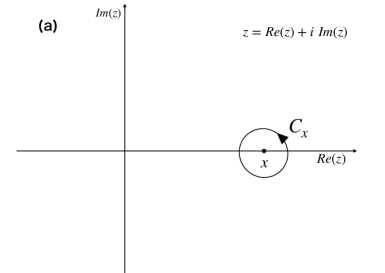
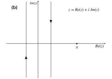
Figure 1: (a) :The contour for $f^{(n)}(x)$ and $g^{(n)}(x)$, (b): A deformed contour.

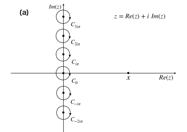
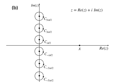
Figure 2: (a): Contours for $f^{(n)}(x)$, (b): Contours for $g^{(n)}(x)$.

The Cauchy formula gives

$$f^{(n)}(x) = n!\sum_{k=-\infty}^{\infty}\ointclockwise_{C_{i\pi k}}\frac{dz}{2\pi i}\frac{z\cosh z}{(z-x)^{n+1}(z-ik\pi)(\sinh z)^{\prime}}$$ (33)

$$= n!\sum_{k=-\infty}^{\infty}\ointclockwise_{C_{i\pi k}}\frac{dz}{2\pi i}\frac{i\pi k}{(i\pi k-x)^{n+1}(z-i\pi k)}$$

$$= -\frac{n!}{(i\pi)^{n}}\sum_{k=1}^{\infty}\Big{[}\frac{k}{(k+ix/\pi)^{n+1}}+{\rm c.c.}\Big{]}$$

$$= -\frac{n!}{(i\pi)^{n}}[-ix/\pi\zeta(n+1,ix/\pi)+\zeta(n,ix/\pi)+{\rm c.c.}],$$

where $\zeta(s,z)$ is the Hurwitz zeta function defined by

$$\zeta(s,z):=\sum_{k=1}^{\infty}\frac{1}{(k+z)^{s}},$$

for $Res>1$ and $z\notin\mathbb{Z}^{-}$, where $\mathbb{Z}^{-}$ is the set of negative integers. Note that

$$f_{n}^{(n)}(x) = f^{(n)}(x)-f^{(n)}(0)$$ (34)

$$= -\frac{n!}{(i\pi)^{n}}\sum_{k=1}^{\infty}\Big{[}\frac{k}{(k+ix/\pi)^{n+1}}+{\rm c.c.}-\frac{2k}{k^{n+1}}\Big{]}$$

$$= (-1)^{n/2}\ \frac{2n!}{\pi^{n}}\sum_{k=1}^{\infty}k^{-n}[1-r_{k}(x)^{-n-1}\cos(n+1)\theta_{k}(x)],$$

where $r_{k}(x)\exp i\theta_{k}(x):=1+ix/(\pi k)$. Note that

$$r_{k}(x)=\sqrt{1+x^{2}/(\pi k)^{2}}\geq 1,$$

which implies

$$1-r_{k}(x)^{-n-1}\cos(n+1)\theta_{k}(x)\geq 0.$$

Therefore, the expression (34) implies that for any $x>0$, $f_{n}^{(n)}(x)\geq 0$ for even $n/2$, and $f_{n}^{(n)}(x)\leq 0$ for odd $n/2$. Since differential coefficients of $f_{n}$ at the origin vanish

$$f_{n}(0)=0=f_{n}^{\prime}(0)=f_{n}^{\prime\prime}(0)=\cdots=f_{n}^{(n-1)}(0).$$

Therefore, $f_{n}(x)\leq 0$ for an odd $n/2$, and $f_{n}(x)\geq 0$ for an even $n/2$.

Next, we prove the sign definiteness of the function $g_{n}(x)$. Since $g_{n}(x)$ is an even function, it is sufficient to show the definiteness of $g_{n}(x)$ for $x\geq 0.$ Let $x$ be a nonnegative number and $n$ be a nonnegative even integer. The $n$-th order derivative of the function $g$ is represented in the following contour integral around $x$ depicted in Figure 1 (a)

$$g^{(n)}(x)=n!\ointctrclockwise_{C_{x}}\frac{dz}{2\pi i}\frac{g(z)}{(z-x)^{n+1}}=n!\sum_{k=-\infty}^{\infty}\ointclockwise_{C_{i\pi(k+1/2)}}\frac{dz}{2\pi i}\frac{\sinh z}{(z-x)^{n+1}z\cosh z}.$$ (35)

Note that the contour depicted in Figure 1 (a) can be deformed into that depicted in Figure 1 (b). Thus, the contour integral (35) is rewritten into that along other contours depicted in Figure 2 (b) . As in the calculation for $f_{n}^{(n)}(x)$, $g_{n}^{(n)}(x)$ can be obtained as

$$g_{n}^{(n)}(x) = g^{(n)}(x)-g^{(n)}(0)$$ (36)

$$= -\frac{n!}{(i\pi)^{n+2}}\sum_{k=1}^{\infty}\Big{[}\frac{1}{(k-1/2+ix/\pi)^{n+1}(k-1/2)}+{\rm c.c.}-\frac{2}{(k-1/2)^{n+2}}\Big{]}$$

$$= (-1)^{n/2+1}\ \frac{2n!}{\pi^{n+2}}\sum_{k=1}^{\infty}(k-1/2)^{-n-2}[1-s_{k}(x)^{-n-1}\cos(n+1)\phi_{k}(x)],$$

where $s_{k}(x)\exp i\phi_{k}(x):=1+ix/[\pi(k-1/2)]$. This implies that $g_{n}^{(n)}(x)\geq 0$ for an odd $n/2$, and $g_{n}^{(n)}(x)\leq 0$ for an even $n/2$. Since differential coefficients of $g_{n}$ at the origin vanish

$$g_{n}(0)=0=g_{n}^{\prime}(0)=g_{n}^{\prime\prime}(0)=\cdots=g_{n}^{(n-1)}(0).$$

Therefore, $g_{n}(x)\geq 0$ for an odd $n/2$, and $f_{n}(x)\leq 0$ for an even $n/2$.

Finally, we prove the sign definiteness of the function $h_{n}(x)$. Since $h_{n}(x)$ is an even function, it is sufficient to show the definiteness of $h_{n}(x)$ for $x\in[0,1).$ The $n$-th order derivative of the function $h(x)$ can be represented in terms of the following contour integral around $x$ depicted in Figure 3 (a)

$$h^{(n)}(x)=n!\ointctrclockwise_{C_{x}}\frac{dz}{2\pi i}\frac{h(z)}{(z-x)^{n+1}}=n!\ointctrclockwise_{C_{x}}\frac{dz}{2\pi i}\frac{z}{(z-x)^{n+1}\log(1+z)/(1-z)}.$$ (37)

Note that the logarithmic function in the integrand has a branch cut $Rez\leq-1,\ Rez\geq 1,$ on the real axis $Imz=0$, as depicted in Figure 3 (b). Rewrite this integration in terms of $w=1/z$

$$h^{(n)}(x) = -n!\ointclockwise_{C_{1/x}}\frac{dw}{2\pi iw^{2}}\frac{w^{-1}}{(w^{-1}-x)^{n+1}\log(1+w^{-1})/(1-w^{-1})}$$ (38)

$$= -n!\ointclockwise_{C_{1/x}}\frac{dw}{2\pi i}\frac{w^{n-2}}{(1-xw)^{n+1}\log(w+1)/(w-1)}.$$

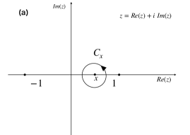
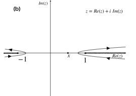
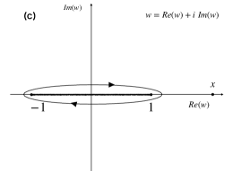
Figure 3: (a): Contour for $h^{(n)}(x)$, (b): Deformed contour, (c): integration over $w=1/z$.

Note that the logarithmic function in the integrand has a branch cut $-1\leq Rew\leq 1,$ on the real axis $Imw=0$,as depicted in Figure 3 (c). This implies

$$h^{(n)}(x) = -n!\int_{-1}^{1}\frac{dw}{2\pi i}\frac{w^{n-2}}{(1-xw)^{n+1}}\Big{[}\frac{1}{\log(1+w)/(1-w)-\pi i}-\frac{1}{\log(1+w)/(1-w)+\pi i}\Big{]}$$ (39)

$$= -n!\int_{-1}^{1}dw\frac{w^{n-2}}{(1-xw)^{n+1}[|\log(1+w)/(1-w)|^{2}+\pi^{2}]}\leq 0,$$

for any $x\in(-1,1).$ This fact and $h_{n}^{(m)}(0)=0$ for any integer $m\in[0,n]$ imply $h_{n}(x)\leq 0$ for any $x\in[0,1)$. This completes the proof. $\Box$

Proof of Theorem 1.

For a bounded linear operator $A$,

$$\frac{1}{2}\langle\{A^{\dagger},A\}\rangle-(A^{\dagger},A)=\int_{-\infty}^{\infty}d\omega\Big{(}\frac{1}{2}-\frac{1}{\beta\omega}\tanh\frac{\beta\omega}{2}\Big{)}Q_{A^{\dagger},A}(\omega)$$

$$=\int_{-\infty}^{\infty}\frac{d\omega}{\beta\omega}\tanh\frac{\beta\omega}{2}\Big{(}\frac{\beta\omega}{2}\coth\frac{\beta\omega}{2}-1\Big{)}Q_{A^{\dagger},A}(\omega).$$ (40)

For a positive odd $n/2$, Lemma 6, Lemma 3, Lemma 5 and $Q_{A^{\dagger},A}(\omega)\geq 0$ imply

$$\frac{1}{2}\langle\{A^{\dagger},A\}\rangle-(A^{\dagger},A)\leq\int_{-\infty}^{\infty}\frac{d\omega}{\beta\omega}\tanh\frac{\beta\omega}{2}\sum_{k=2}^{n}\frac{f^{(k)}(0)}{k!}\Big{(}\frac{\beta\omega}{2}\Big{)}^{k}Q_{A^{\dagger},A}(\omega)$$

$$=\int_{-\infty}^{\infty}\frac{d\omega}{2}\omega\tanh\frac{\beta\omega}{2}\sum_{k=1}^{n/2}\frac{f^{(2k)}(0)}{(2k)!}\Big{(}\frac{\beta}{2}\Big{)}^{2k-1}\omega^{2k-2}Q_{A^{\dagger},A}(\omega)$$

$$=\int_{-\infty}^{\infty}\frac{d\omega}{2}\omega\tanh\frac{\beta\omega}{2}\sum_{k=1}^{n/2}\frac{f^{(2k)}(0)}{(2k)!}\Big{(}\frac{\beta}{2}\Big{)}^{2k-1}Q_{{C_{A}^{k-1}}^{\dagger},C_{A}^{k-1}}(\omega)$$

$$=\sum_{k=1}^{n/2}\frac{f^{(2k)}(0)}{2(2k)!}\Big{(}\frac{\beta}{2}\Big{)}^{2k-1}\langle[{C_{A}^{k-1}}^{\dagger},[H,C_{A}^{k-1}]]\rangle.$$ (41)

Since $(n+2)/2$ is even, Lemma 6 and $Q_{A^{\dagger},A}(\omega)\geq 0$ imply

$$\frac{1}{2}\langle\{A^{\dagger},A\}\rangle-(A^{\dagger},A)\geq\int_{-\infty}^{\infty}\frac{d\omega}{\beta\omega}\tanh\frac{\beta\omega}{2}\sum_{k=2}^{n+2}\frac{f^{(k)}(0)}{k!}\Big{(}\frac{\beta\omega}{2}\Big{)}^{k}Q_{A^{\dagger},A}(\omega)$$

$$=\int_{-\infty}^{\infty}\frac{d\omega}{2}\omega\tanh\frac{\beta\omega}{2}\sum_{k=1}^{n/2+1}\frac{f^{(2k)}(0)}{(2k)!}\Big{(}\frac{\beta}{2}\Big{)}^{2k-1}\omega^{2k-2}Q_{A^{\dagger},A}(\omega)$$

$$=\int_{-\infty}^{\infty}\frac{d\omega}{2}\omega\tanh\frac{\beta\omega}{2}\sum_{k=1}^{n/2+1}\frac{f^{(2k)}(0)}{(2k)!}\Big{(}\frac{\beta}{2}\Big{)}^{2k-1}Q_{{C_{A}^{k-1}}^{\dagger},C_{A}^{k-1}}(\omega)$$

$$=\sum_{k=1}^{n/2+1}\frac{f^{(2k)}(0)}{2(2k)!}\Big{(}\frac{\beta}{2}\Big{)}^{2k-1}\langle[{C_{A}^{k-1}}^{\dagger},[H,C_{A}^{k-1}]]\rangle$$ (42)

These and $[H,C_{A}^{k-1}]=C_{A}^{k}$ complete the proof of Theorem 1. $\Box$

Proof of Theorem 2.

For a bounded linear operator $A$,

$$(A^{\dagger},A)=\int_{-\infty}^{\infty}d\omega\frac{1}{\beta\omega}\tanh\frac{\beta\omega}{2}Q_{A^{\dagger},A}(\omega)=\int_{-\infty}^{\infty}\frac{d\omega}{2}g\Big{(}\frac{\beta\omega}{2}\Big{)}Q_{A^{\dagger},A}(\omega).$$ (43)

For a nonnegative even $n/2$, $(n+2)/2$ is an odd integer, Lemma 6, Lemma 3, Lemma 5 and $Q_{A^{\dagger},A}(\omega)\geq 0$ imply

$$(A^{\dagger},A)\geq\int_{-\infty}^{\infty}\frac{d\omega}{2}\sum_{k=0}^{n+2}\frac{g^{(k)}(0)}{k!}\Big{(}\frac{\beta\omega}{2}\Big{)}^{k}Q_{A^{\dagger},A}(\omega)=\int_{-\infty}^{\infty}\frac{d\omega}{2}\sum_{k=0}^{n/2+1}\frac{g^{(2k)}(0)}{(2k)!}\Big{(}\frac{\beta\omega}{2}\Big{)}^{2k}Q_{A^{\dagger},A}(\omega)$$

$$=\int_{-\infty}^{\infty}\frac{d\omega}{2}\sum_{k=0}^{n/2+1}\frac{g^{(2k)}(0)}{(2k)!}\Big{(}\frac{\beta}{2}\Big{)}^{2k}Q_{{C_{A}^{k}}^{\dagger},C_{A}^{k}}(\omega)=\sum_{k=0}^{n/2+1}\frac{g^{(2k)}(0)}{2(2k)!}\Big{(}\frac{\beta}{2}\Big{)}^{2k}\langle\{{C_{A}^{k}}^{\dagger},C_{A}^{k}\}\rangle.$$ (44)

Since $n/2$ is even, Lemma 6 and $Q_{A^{\dagger},A}(\omega)\geq 0$ imply

$$(A^{\dagger},A)\leq\int_{-\infty}^{\infty}\frac{d\omega}{2}\sum_{k=0}^{n}\frac{g^{(k)}(0)}{k!}\Big{(}\frac{\beta\omega}{2}\Big{)}^{k}Q_{A^{\dagger},A}(\omega)=\int_{-\infty}^{\infty}\frac{d\omega}{2}\sum_{k=1}^{n/2}\frac{g^{(2k)}(0)}{(2k)!}\Big{(}\frac{\beta\omega}{2}\Big{)}^{2k}Q_{A^{\dagger},A}(\omega)$$

$$=\int_{-\infty}^{\infty}\frac{d\omega}{2}\sum_{k=0}^{n/2}\frac{g^{(2k)}(0)}{(2k)!}\Big{(}\frac{\beta}{2}\Big{)}^{2k}Q_{{C_{A}^{k}}^{\dagger},C_{A}^{k}}(\omega)=\sum_{k=0}^{n/2}\frac{g^{(2k)}(0)}{2(2k)!}\Big{(}\frac{\beta}{2}\Big{)}^{2k}\langle\{{C_{A}^{k}}^{\dagger},C_{A}^{k}\}\rangle.$$ (45)

This completes the proof of Theorem 2. $\Box$

Proof of Theorem 3.

For a bounded linear operator $A$,

$$\langle[A^{\dagger},[H,A]]\rangle=\int_{-\infty}^{\infty}d\omega\omega\tanh\frac{\beta\omega}{2}Q_{A^{\dagger},A}(\omega)=\int_{-\infty}^{\infty}d\omega\frac{\beta}{2}g\Big{(}\frac{\beta\omega}{2}\Big{)}\omega^{2}Q_{A^{\dagger},A}(\omega).$$ (46)

For a nonnegative even $n/2$, $(n+2)/2$ is an odd integer, Lemma 6, Lemma 3, Lemma 5 and $Q_{A^{\dagger},A}(\omega)\geq 0$ imply

$$\langle[A^{\dagger},[H,A]]\rangle\geq\int_{-\infty}^{\infty}d\omega\frac{\beta}{2}\sum_{k=0}^{n+2}\frac{g^{(k)}(0)}{k!}\Big{(}\frac{\beta\omega}{2}\Big{)}^{k}\omega^{2}Q_{A^{\dagger},A}(\omega)=\int_{-\infty}^{\infty}d\omega\sum_{k=0}^{n/2+1}\frac{g^{(2k)}(0)}{(2k)!}\Big{(}\frac{\beta}{2}\Big{)}^{2k+1}\omega^{2k+2}Q_{A^{\dagger},A}(\omega)$$

$$=\int_{-\infty}^{\infty}d\omega\sum_{k=0}^{n/2+1}\frac{g^{(2k)}(0)}{(2k)!}\Big{(}\frac{\beta}{2}\Big{)}^{2k+1}Q_{{C_{A}^{k+1}}^{\dagger},C_{A}^{k+1}}(\omega)=\sum_{k=0}^{n/2+1}\frac{g^{(2k)}(0)}{(2k)!}\Big{(}\frac{\beta}{2}\Big{)}^{2k+1}\langle\{{C_{A}^{k+1}}^{\dagger},C_{A}^{k+1}\}\rangle.$$ (47)

Since $n/2$ is even, Lemma 6 and $Q_{A^{\dagger},A}(\omega)\geq 0$ imply

$$\langle[A^{\dagger},[H,A]]\rangle\leq\int_{-\infty}^{\infty}d\omega\sum_{k=0}^{n}\frac{g^{(k)}(0)}{k!}\Big{(}\frac{\beta}{2}\Big{)}^{k+1}\omega^{k+2}Q_{A^{\dagger},A}(\omega)=\int_{-\infty}^{\infty}d\omega\sum_{k=1}^{n/2}\frac{g^{(2k)}(0)}{(2k)!}\Big{(}\frac{\beta}{2}\Big{)}^{2k+1}\omega^{2k+2}Q_{A^{\dagger},A}(\omega)$$

$$=\int_{-\infty}^{\infty}d\omega\sum_{k=0}^{n/2}\frac{g^{(2k)}(0)}{(2k)!}\Big{(}\frac{\beta}{2}\Big{)}^{2k+1}Q_{{C_{A}^{k+1}}^{\dagger},C_{A}^{k+1}}(\omega)=\sum_{k=0}^{n/2}\frac{g^{(2k)}(0)}{(2k)!}\Big{(}\frac{\beta}{2}\Big{)}^{2k+1}\langle\{{C_{A}^{k+1}}^{\dagger},C_{A}^{k+1}\}\rangle.$$ (48)

This completes the proof of Theorem 3. $\Box$

Proof of Theorem 4.

The spectral representation of the Duhamel function for bounded linear operators $A^{\dagger},A$ is

$$(A^{\dagger},A)=\int_{-\infty}^{\infty}\frac{d\omega}{\beta\omega}\tanh\frac{\beta\omega}{2}Q_{A^{\dagger},A}(\omega)=\int_{-\infty}^{\infty}\frac{d\omega}{2}g\Big{(}\frac{\beta\omega}{2}\Big{)}Q_{A^{\dagger},A}(\omega),$$ (49)

where $g:\mathbb{R}\to\mathbb{R}$ defined by (2). Define an integration measure

$$d\mu(\omega):=\frac{d\omega}{2}g\Big{(}\frac{\beta\omega}{2}\Big{)}\frac{Q_{A^{\dagger},A}(\omega)}{(A^{\dagger},A)}.$$ (50)

Note that

$$\int_{-\infty}^{\infty}d\mu(\omega)=1.$$

The Jensen inequality for the convex function $f:\mathbb{R}\to\mathbb{R}$ defined by (2) implies

$$f\Big{(}\frac{\langle[A^{\dagger},A]\rangle}{2(A^{\dagger},A)}\Big{)}=f\Big{(}\int_{-\infty}^{\infty}d\mu(\omega)\frac{\beta\omega}{2}\Big{)}\leq\int_{-\infty}^{\infty}d\mu(\omega)f\Big{(}\frac{\beta\omega}{2}\Big{)}=\frac{\langle\{A^{\dagger},A\}\rangle}{2(A^{\dagger},A)}.$$ (51)

This inequality gives

$$\frac{2(A^{\dagger},A)}{\langle[A^{\dagger},A]\rangle}\tanh\frac{\langle[A^{\dagger},A]\rangle}{2(A^{\dagger},A)}=g\Big{(}\frac{\langle[A^{\dagger},A]\rangle}{2(A^{\dagger},A)}\Big{)}\geq\frac{2(A^{\dagger},A)}{\langle\{A^{\dagger},A\}\rangle},$$ (52)

then

$$\tanh\frac{\langle[A^{\dagger},A]\rangle}{2(A^{\dagger},A)}\geq\frac{\langle[A^{\dagger},A]\rangle}{\langle\{A^{\dagger},A\}\rangle}.$$ (53)

This inequality can be represented in terms of the function $h:(-1,1)\to\mathbb{R}$ defined by (2)

$$\frac{(A^{\dagger},A)}{\langle\{A^{\dagger},A\}\rangle}\leq\frac{\frac{\langle[A^{\dagger},A]\rangle}{\langle\{A^{\dagger},A\}\rangle}}{2\tanh^{-1}\frac{\langle[A^{\dagger},A]\rangle}{\langle\{A^{\dagger},A\}\rangle}}=h\Big{(}\frac{\langle[A^{\dagger},A]\rangle}{\langle\{A^{\dagger},A\}\rangle}\Big{)},$$ (54)

which is obtained by Roepstorff [3]. Lemma 6 gives an upper bound on the right hand side

$$h\Big{(}\frac{\langle[A^{\dagger},A]\rangle}{\langle\{A^{\dagger},A\}\rangle}\Big{)}\leq\sum_{k=0}^{n}\frac{h^{(k)}(0)}{k!}\Big{(}\frac{\langle[A^{\dagger},A]\rangle}{\langle\{A^{\dagger},A\}\rangle}\Big{)}^{k}.$$

Therefore,

$$\frac{(A^{\dagger},A)}{\langle\{A^{\dagger},A\}\rangle}\leq\sum_{k=0}^{n}\frac{h^{(k)}(0)}{k!}\Big{(}\frac{\langle[A^{\dagger},A]\rangle}{\langle\{A^{\dagger},A\}\rangle}\Big{)}^{k},$$

is obtained. This completes the proof of Theorem 4. $\Box$

4 Applications to the Transverse Field Sherrington-Kirkpatrick Model

Here, we study quantum spin systems with random interactions. Let $N$ be a positive integer and a site index $i\ (\leq N)$ is also a positive integer. A sequence of spin operators $(\sigma^{w}_{i})_{w=x,y,z,1\leq i\leq N}$ on a Hilbert space ${\cal H}:=\bigotimes_{i=1}^{N}{\cal H}_{i}$ is defined by a tensor product of the Pauli matrix $\sigma^{w}$ acting on ${\cal H}_{i}\simeq{\mathbb{C}}^{2}$ and unities. These operators are self-adjoint and satisfy the commutation relation

$$[\sigma_{k}^{y},\sigma_{j}^{z}]=2i\delta_{k,j}\sigma_{j}^{x},\ \ \ \ \ [\sigma_{k}^{z},\sigma_{j}^{x}]=2i\delta_{k,j}\sigma_{j}^{y},\ \ \ \ \ [\sigma_{k}^{x},\sigma_{j}^{y}]=2i\delta_{k,j}\sigma_{j}^{z},$$

and each spin operator satisfies

$$(\sigma_{j}^{w})^{2}={\bf 1}.$$

The Sherrington-Kirkpatrick (SK) model is well-known as a disordered classical spin system [11]. The transverse field SK model is a simple quantum extension. Here, we study a magnetization process for a local field in these models. Consider the following Hamiltonian with coupling constants $b_{1},h\in{\mathbb{R}}$

$$H_{N}(\sigma,b_{1},g,h):=-\frac{1}{\sqrt{N}}\sum_{1\leq i<j\leq N}g_{i,j}\sigma_{i}^{z}\sigma_{j}^{z}-\sum_{j=1}^{N}h\sigma_{j}^{z}-\sum_{j=1}^{N}b_{1}\sigma_{j}^{x},$$ (55)

where $g=(g_{i,j})_{1\leq i<j\leq N}$ is a sequence of independent standard Gaussian random variables obeying a probability density function

$$p(g):=\prod_{1\leq i<j\leq N}\frac{1}{\sqrt{2\pi}}e^{-\frac{g_{i,j}^{2}}{2}}$$ (56)

The Hamiltonian is invariant under $\mathbb{Z}_{2}$-symmetry $U\sigma_{i}^{z}U^{\dagger}=-\sigma_{i}^{z}$ for the discrete unitary transformation $U:=\prod_{1\leq i\leq N}\sigma_{i}^{x}$ for $h=0$. For a positive $\beta$, the partition function is defined by

$$Z_{N}(\beta,b_{1},g,h):={\rm Tr}e^{-\beta H_{N}(\sigma,b_{1},g,h)},$$ (57)

where the trace is taken over the Hilbert space ${\cal H}$. Here, we define a square root interpolation for the transverse field SK model, as for the SK model given by Guerra and Talagrand [9, 10]. Let $z=(z_{j})_{1\leq j\leq N}$ be a sequence of independent standard Gaussian random variables. This method gives a variational solution of specific free energy. Consider the following interpolated Hamiltonian with parameters $s\in[0,1]$, $b(s):=b_{1}s+b_{0}(1-s)$ for $b_{0}\in\mathbb{R}$ and $q\in[0,1]$

$$H(s,\sigma):=-\sqrt{\frac{s}{N}}\sum_{1\leq i<j\leq N}g_{i,j}\sigma_{i}^{z}\sigma_{j}^{z}-\sum_{j=1}^{N}(\sqrt{q(1-s)}z_{j}+h)\sigma_{j}^{z}-\sum_{j=1}^{N}b(s)\sigma_{j}^{x}.$$ (58)

Define an interpolated function $\varphi_{N}(s)$

$$\varphi_{N}(s):=\frac{1}{N}\mathbb{E}\log{\rm Tr}e^{-\beta H(s,\sigma)}$$ (59)

where $\mathbb{E}$ denotes the expectation over all Gaussian random variables $(g_{i,j})_{1\leq i<j\leq N}$ and $(z_{i})_{1\leq i\leq N}$. Note that $\varphi_{N}(1)$ is given by

$$\varphi_{N}(1)=\frac{1}{N}\mathbb{E}\log Z_{N}(\beta,b_{1},g,h),$$

which is proportional to the specific free energy of the transverse field SK model. Let $f$ be an arbitrary function of a sequence of spin operators $\sigma=(\sigma_{i}^{w})_{w=x,y,z,1\leq i\leq N}$. The expectation of $f$ in the Gibbs state is given by

$$\langle f(\sigma)\rangle_{s}=\frac{{\rm Tr}f(\sigma)e^{-\beta H(s,\sigma)}}{{\rm Tr}e^{-\beta H(s,\sigma)}}.$$ (60)

The derivative of $\varphi_{N}(s)$ with respect to $s$ is given by

$$\varphi^{\prime}_{N}(s)=\frac{\beta}{2N^{\frac{3}{2}}\sqrt{s}}\sum_{1\leq<j\leq N}\mathbb{E}g_{i,j}\langle\sigma_{i}^{z}\sigma_{j}^{z}\rangle_{s}-\frac{\beta\sqrt{q}}{2N\sqrt{1-s}}\sum_{i=1}^{N}\mathbb{E}z_{i}\langle\sigma_{i}^{z}\rangle_{s}+\frac{\beta b^{\prime}(s)}{N}\sum_{i=1}^{N}\mathbb{E}\langle\sigma_{i}^{x}\rangle_{s}.$$ (61)

The identities for the Gaussian random variables $g_{i,j}$ and $z_{i}$

$$g_{i,j}p(g,z)=-\frac{\partial p}{\partial g_{i,j}},\ \ \ z_{i}p(g,z)=-\frac{\partial p}{\partial z_{i}}$$

and the integration by parts imply

$$\varphi^{\prime}_{N}(s) = \frac{\beta^{2}}{2N^{2}}\sum_{1\leq<j\leq N}\mathbb{E}[(\sigma_{i}^{z}\sigma_{j}^{z},\sigma_{i}^{z}\sigma_{j}^{z})_{s}-\langle\sigma_{i}^{z}\sigma_{j}^{z}\rangle_{s}^{2}]-\frac{\beta^{2}q}{2N}\sum_{i=1}^{N}\mathbb{E}[(\sigma_{i}^{z},\sigma_{i}^{z})_{s}-\langle\sigma_{i}^{z}\rangle_{s}^{2}]+\frac{\beta b^{\prime}(s)}{N}\sum_{i=1}^{N}\mathbb{E}\langle\sigma_{i}^{x}\rangle_{s}$$ (62)

$$= \frac{\beta^{2}(N-1)}{4N}[\mathbb{E}(\sigma_{1}^{z}\sigma_{2}^{z},\sigma_{1}^{z}\sigma_{2}^{z})_{s}-1]-\frac{\beta^{2}q}{2}[\mathbb{E}(\sigma_{1}^{z},\sigma_{1}^{z})_{s}-1]+\beta b^{\prime}(s)\mathbb{E}\langle\sigma_{1}^{x}\rangle_{s}$$

$$+ \frac{\beta^{2}}{4}(1-q)^{2}-\frac{\beta^{2}}{4}\mathbb{E}\langle(R_{1,2}-q)^{2}\rangle_{s},$$

where the overlap operator $R_{a,b}$ is defined by

$$R_{a,b}:=\frac{1}{N}\sum_{i=1}^{N}\sigma_{i}^{z,a}\sigma_{i}^{z,b},$$

for independent replicated Pauli operators $\sigma_{i}^{z,a}\ (a=1,2,\cdots,n)$ obeying the same Gibbs state with the replica Hamiltonian

$$H(s,\sigma^{1},\cdots,\sigma^{n}):=\sum_{a=1}^{n}H(s,\sigma^{a}).$$

This Hamiltonian is invariant under permutation of replica spins. This permutation symmetry is known to be the replica symmetry. The order operator $R_{a,b}$ measures the replica symmetry breaking as an order operator. In the identity (62), we use an upper bound $\mathbb{E}(\sigma_{1}^{z}\sigma_{2}^{z},\sigma_{1}^{z}\sigma_{2}^{z})_{s}\leq 1$ given by the right-hand side of the inequality (9), and the lower bound on the Duhamel function $(\sigma_{1}^{z},\sigma_{1}^{z})$

$$-\frac{\beta^{2}q}{2}\mathbb{E}[(\sigma_{1}^{z},\sigma_{1}^{z})_{s}-1]\leq\frac{\beta^{4}q}{48}\mathbb{E}\langle\{[H,\sigma_{1}^{z}]^{\dagger},[H,\sigma_{1}^{z}]\}\rangle_{s}=\frac{\beta^{4}q}{6}b(s)^{2},$$

given by the left-hand side of the inequality (9). Then, we have

$$\varphi^{\prime}_{N}(s) \leq \frac{\beta^{4}q}{48}\mathbb{E}\langle\{[H,\sigma_{1}^{z}]^{\dagger},[H,\sigma_{1}^{z}]\}\rangle_{s}+\beta b^{\prime}(s)\mathbb{E}\langle\sigma_{1}^{x}\rangle_{s}+\frac{\beta^{2}}{4}(1-q)^{2}-\frac{\beta^{2}}{4}\mathbb{E}\langle(R_{1,2}-q)^{2}\rangle_{s}$$ (63)

$$= \frac{\beta^{4}q}{6}b(s)^{2}+\beta b^{\prime}(s)\mathbb{E}\langle\sigma_{1}^{x}\rangle_{s}+\frac{\beta^{2}}{4}(1-q)^{2}-\frac{\beta^{2}}{4}\mathbb{E}\langle(R_{1,2}-q)^{2}\rangle_{s}$$

$$\leq \frac{\beta^{4}q}{6}b(s)^{2}+\beta b^{\prime}(s)\tanh\beta b(s)+\frac{\beta^{2}}{4}(1-q)^{2},$$

where an upper bound $\tanh\beta b(s)\geq\langle\sigma_{1}^{x}\rangle_{s}$ has been used as shown by Leschke, Manai, Ruder and Warzel [8]. The bound on the Duhamel function $(\sigma_{1}^{z},\sigma_{1}^{z})_{s}$ can be obtained also from the Falk-Bruch inequality [2] and our result for $g(z)$ defined by (2), instead of the simple use of the inequality (9). For $\Phi(r\tanh r):=\tanh r/r=g(r)$,

$$(\sigma_{1}^{z},\sigma_{1}^{z})_{s}\geq\Phi\biggl{(}\frac{\langle[\sigma_{1}^{z},[\beta H,\sigma_{1}^{z}]]\rangle_{s}}{4}\biggr{)},$$

is obtained by Leschke, Manai, Ruder and Warzel as a corollary of the Falk-Bruch inequality [8]. The equality and the inequality $\langle[\sigma_{1}^{z},[\beta H,\sigma_{1}^{z}]]\rangle_{s}=4\beta b(s)\langle\sigma_{1}^{x}\rangle_{s}\leq 4\beta b(s)\tanh\beta b(s)$, the monotonicity and the convexity of the function $\Phi$, the definition of $\Phi$ and Lemma 6 give the lower bound on $(\sigma_{1}^{z},\sigma_{1}^{z})_{s}$

$$(\sigma_{1}^{z},\sigma_{1}^{z})_{s}\geq\Phi(\beta b(s)\langle\sigma_{1}^{x}\rangle_{s})\geq\Phi(\beta b(s)\tanh\beta b(s))=g(\beta b(s))\geq 1-\frac{\beta^{2}}{3}b(s)^{2},$$

which gives the same upper bound (63). The advantage of using the new inequality (9) in the present case is that the lower bound on the Duhamel function is easily expressed in terms of the known simple function of $\beta$ and $b(s)$ with far fewer calculations. Although a relation between the Falk-Bruch inequality and the new inequality (9) can be understood in the present specific case, it is difficult to clarify that in general case.

Integration of the inequality (63) over $s\in[0,1]$ gives

$$\varphi_{N}(1) \leq \varphi_{N}(0)+\int_{0}^{1}ds[\frac{\beta^{4}q}{6}b(s)^{2}+\beta b^{\prime}(s)\tanh\beta b(s)+\frac{\beta^{2}}{4}(1-q)^{2}]$$ (64)

$$= \varphi_{N}(0)+\frac{\beta^{4}q}{18}(b_{0}^{2}+b_{0}b_{1}+b_{1}^{2})+\log\frac{\cosh\beta b_{1}}{\cosh\beta b_{0}}+\frac{\beta^{2}}{4}(1-q)^{2}=:\Phi(q,b_{0}).$$

The model at $s=0$ becomes independent spin model, and therefore

$$\varphi_{N}(0)=\mathbb{E}\log{\rm Tr}\exp\beta[(\sqrt{q}z+h)\sigma^{z}+b_{0}\sigma^{x}]=\mathbb{E}\log 2\cosh\beta\sqrt{(\sqrt{q}z+h)^{2}+b_{0}^{2}}.$$ (65)

A variational solution with the best bound is obtained by minimizing the right hand side in (64). The minimizer $(q,b_{0})$ should satisfy

$$0 = \frac{\partial}{\partial q}\Phi(q,b_{0})=\mathbb{E}\frac{\beta z(\sqrt{q}z+h)\tanh\beta\sqrt{(\sqrt{q}z+h)^{2}+b_{0}^{2}}}{2\sqrt{q}\sqrt{(\sqrt{q}z+h)^{2}+b_{0}^{2}}}+\frac{\beta^{4}}{18}(b_{0}^{2}+b_{0}b_{1}+b_{1}^{2})-\frac{\beta^{2}}{2}(1-q)$$ (66)

$$= \mathbb{E}\frac{\beta^{2}(\sqrt{q}z+h)^{2}}{2[(\sqrt{q}z+h)^{2}+b_{0}^{2}]\cosh^{2}\beta\sqrt{(\sqrt{q}z+h)^{2}+b_{0}^{2}}}+\mathbb{E}\frac{\beta b_{0}^{2}\tanh\beta\sqrt{(\sqrt{q}z+h)^{2}+b_{0}^{2}}}{2[(\sqrt{q}z+h)^{2}+b_{0}^{2}]^{\frac{3}{2}}}$$

$$+ \frac{\beta^{4}}{18}(b_{0}^{2}+b_{0}b_{1}+b_{1}^{2})-\frac{\beta^{2}}{2}(1-q),$$

$$0 = \frac{\partial}{\partial b_{0}}\Phi(q,b_{0})=\mathbb{E}\frac{\beta b_{0}\tanh\beta\sqrt{(\sqrt{q}z+h)^{2}+b_{0}^{2}}}{\sqrt{(\sqrt{q}z+h)^{2}+b_{0}^{2}}}-\beta\tanh\beta b_{0}+\frac{\beta^{4}q}{18}(2b_{0}+b_{1}),$$ (67)

where the following integration by parts has been used to obtain the equation (66)

$$\mathbb{E}\frac{\beta z(\sqrt{q}z+h)\tanh\beta\sqrt{(\sqrt{q}z+h)^{2}+b_{0}^{2}}}{2\sqrt{q}\sqrt{(\sqrt{q}z+h)^{2}+b_{0}^{2}}}=\mathbb{E}\frac{\beta}{\sqrt{q}}\frac{\partial}{\partial z}\frac{(\sqrt{q}z+h)\tanh\beta\sqrt{(\sqrt{q}z+h)^{2}+b_{0}^{2}}}{2\sqrt{(\sqrt{q}z+h)^{2}+b_{0}^{2}}}.$$

This minimizer $(q,b_{0})$ gives the best bound on $\varphi_{N}(1)$ as a variational solution

$$\varphi_{N}(1)\leq\mathbb{E}\log 2\cosh\beta\sqrt{(\sqrt{q}z+h)^{2}+b_{0}^{2}}+\frac{\beta^{4}q}{18}(b_{0}^{2}+b_{0}b_{1}+b_{1}^{2})+\log\frac{\cosh\beta b_{1}}{\cosh\beta b_{0}}+\frac{\beta^{2}}{4}(1-q)^{2}.$$ (68)

Note that the equation (67) has a solution $b_{0}=0$ in the classical limit $b_{1}\to 0$. In this case the equation (66) becomes

$$q=\mathbb{E}\tanh^{2}\beta(\sqrt{q}z+h).$$ (69)

Then, the solution (68) is identical to the SK solution [11] in the classical limit $b_{1}\to 0$. In the classical case $b_{1}=0$, it is conjectured that the replica symmetry is preserved with

$$\lim_{N\to\infty}\mathbb{E}\langle(R_{1,2}-q)^{2}\rangle_{1}=0,$$

and the SK solution of the specific free energy is exact for

$$\mathbb{E}\frac{\beta^{2}}{\cosh^{4}\beta(\sqrt{q}z+h)}\leq 1,$$

whose boundary is called the Almeida-Thouless line [12]. Recently, Chen has proven rigorously that the SK solution is exact for independent centered Gaussian random external fields, instead of the uniform field $h$ [13]. For the uniform field $h\neq 0$, it still remains a conjecture.

Consider a simple case $h=0$, where the model has the $\mathbb{Z}_{2}$ symmetry. If the replica symmetric solution $q=0$ is assumed in this case, the equation (66) becomes

$$0=\tanh\beta b_{0}-\beta b_{0}+\frac{\beta^{3}}{9}b_{0}(b_{0}^{2}+b_{0}b_{1}+b_{1}^{2}),$$ (70)

which fixes $b_{0}$, and the equation (67) is valid for any $b_{0}$. Therefore, the $\mathbb{Z}_{2}$ and replica symmetric variational solution of the specific free energy is given by

$$-\varphi_{N}(1)/\beta\geq-\frac{1}{\beta}\log 2\cosh\beta b_{1}-\frac{\beta}{4},$$ (71)

under the assumption $q=0$ for $h=0$. This lower bound can be compared to results obtained in other literatures. Leschke, Rothlauf, Ruder and Spitzer evaluate the specific free energy in a different rigorous method based on the annealed free energy [14]. They first give a simple estimate of its lower bound in the high temperature region $\beta<1$ [14]. This lower bound is exactly the same as the right hand side of the inequality (71) in the infinite volume limit. In addition, they obtain a corrected estimate in a high temperature expansion [14]. Although this estimate might be better, the correction is quite small. The specific free energy $f_{\rm st}(\beta,b_{1},h)$ obtained by the replica trick with the static approximation [15] is

$$-\varphi_{N}(1)/\beta\simeq f_{\rm st}(\beta,b_{1},h=0)=-\frac{1}{\beta}\log 2\cosh\beta b_{1},$$ (72)

which violates a rigorous upper bound

$$-\varphi_{N}(1)/\beta\leq-\frac{1}{\beta}\log 2\cosh\beta b_{1}-\frac{\beta}{8}\Big{(}\frac{1}{\cosh^{2}\beta b_{1}}+\frac{\tanh\beta b_{1}}{\beta b_{1}}\Big{)},$$ (73)

given by Leschke, Rothlauf, Ruder and Spitzer[14]. For a strong field $h\gg 1$, however, the approximate specific free energy

$$f_{\rm st}(\beta,b_{1},h)\simeq-\frac{1}{\beta}\mathbb{E}\log 2\cosh\beta\sqrt{(\sqrt{q}z+h)^{2}+b_{1}^{2}},$$

must be a good approximation, since the following deviation of the strong field limit vanishes

$$\lim_{h\to\infty}[\beta f_{\rm st}(\beta,b_{1},h)+\varphi_{N}(1)]=0.$$

On the other hand, the upper bound (68) and $q\to 1$ in this limit give an upper bound on the following deviation

$$\lim_{h\to\infty}[\varphi_{N}(1)-\mathbb{E}\log 2\cosh\beta\sqrt{(\sqrt{q}z+h)^{2}+b_{1}^{2}}]\leq\frac{\beta^{4}}{18}(b_{0}^{2}+b_{0}b_{1}+b_{1}^{2})+\log\frac{\cosh\beta b_{1}}{\cosh\beta b_{0}}=:D,$$

where $b_{0}$ is the solution of the equation

$$\tanh\beta b_{0}-\frac{\beta^{3}}{18}(2b_{0}+b_{1})=0,$$

obtained from (67). Since the relative deviation vanishes

$$\lim_{h\to\infty}D/\varphi_{N}(1)=0,$$

in the strong field limit, the upper bound on $\varphi_{N}(1)$ given by the right hand side of (68) must be a good approximation for $h\gg 1$ as well as the approximate specific free energy $f_{\rm st}(\beta,b_{1},h)$.

Acknowledgments  

C.I. is supported by JSPS (21K03393).

References

- [1] N. N. Bogolubov, Physica 26, Sl (1960).
- [2] H. Falk and L. W. Bruch, Phys. Rev. 180, 442 (1969).
- [3] G. Roepstorff, Commun. Math. Phys. 53, 143 (1977).
- [4] J. G. Brankov and N. S. Tonchev, Cond. Matt. Phys. 14, 13003 (2011).
- [5] A. B. Harris, J. Math. Phys. 8, 1044 (1967).
- [6] B. S. Shastry, J. Phys. A: Math. Gen. 25, L249 (1992).
- [7] N. D. Mermin and H. Wagner, Phys. Rev. Lett. 17, 1133 (1966).
- [8] H. Leschke, C. Manai, R. Ruder, and S. Warzel, Phys. Rev. Lett. 127, 207204 (2021).
- [9] F. Guerra, Fields Inst. Commun. 30, 161 (2001).
- [10] M. Talagrand, Mean field models for spin glasses I, II (Springer, Berlin, 2011).
- [11] D. Sherrington and S. Kirkpatrick, Phys. Rev. Lett. 35, 1792 (1975).
- [12] J. R. L. de Almeida and D. J. Thouless, J. Phys. A: Math. Gen. 11, 983 (1978).
- [13] W. -K. Chen, Electron. Commun. Probab. 26, 1 (2021).
- [14] H. Leschke, S. Rothlauf, R. Ruder and W. Spitzer, J. Stat. Phys. 182, 55 (2021).
- [15] D-H. Kim and J-J. Kim, Phys. Rev. B 66, 054432 (2002).