Quantifying the Variability Collapse of Neural Networks

Abstract

Recent studies empirically demonstrate the positive relationship between the transferability of neural networks and the within-class variation of the last layer features. The recently discovered Neural Collapse (NC) phenomenon provides a new perspective of understanding such last layer geometry of neural networks. In this paper, we propose a novel metric, named Variability Collapse Index (VCI), to quantify the variability collapse phenomenon in the NC paradigm. The VCI metric is well-motivated and intrinsically related to the linear probing loss on the last layer features. Moreover, it enjoys desired theoretical and empirical properties, including invariance under invertible linear transformations and numerical stability, that distinguishes it from previous metrics. Our experiments verify that VCI is indicative of the variability collapse and the transferability of pretrained neural networks.

1 Introduction

The pursuit of powerful models capable of extracting features from raw data and performing well on downstream tasks has been a constant endeavor in the machine learning community (Bommasani et al., 2021). In the past few years, researchers have developed various pretraining methods (Chen et al., 2020; Khosla et al., 2020; Grill et al., 2020; He et al., 2022; Baevski et al., 2022) that enable models to learn from massive real world datasets. However, there is still a lack of systematic understanding regarding the transferability of deep neural networks, i.e., whether they can leverage the information in the pretraining datasets to achieve high performance in downstream tasks (Abnar et al., 2021; Fang et al., 2023).

The performance of a pretrained model is closely related to the quality of the features it produces. The recently proposed concept of neural collapse (NC) (Papyan et al., 2020) provides a paradigmatic way to study the representation of neural networks. According to neural collapse, the last layer features of neural networks adhere to the following rule of variability collapse (NC1): As the training proceeds, the representation of a data point converges to its corresponding class mean. Consequently, the within-class variation of the features converges to zero.

The deep connection between transferability and neural collapse is rooted in the variability collapse criterion. Previous works (Feng et al., 2021; Kornblith et al., 2021; Sariyildiz et al., 2022) empirically find that although models with collapsed last-layer feature representations exhibit better pretraining accuracy, they tend to yield worse performance for downstream tasks. These works give an intuitive explanation that pushing the feature to their class means results in the loss of the diverse structures useful for downstream tasks. Building upon this understanding, researchers design various algorithms (Jing et al., 2021; Kini et al., 2021; Chen et al., 2022; Dubois et al., 2022; Sariyildiz et al., 2023) that either explicitly or implicitly levarage the variability collapse criterion to retain the feature diversity in the pretraining phase, and thereby improve the transferability of the models.

Straightforward as it is stated, the variability criterion is still not thoroughly understood. One fundamental question is how to mathematically quantify variability collapse. Previous works propose variability collapse metrics that are meaningful in specific settings (Papyan et al., 2020; Zhu et al., 2021; Kornblith et al., 2021; Hui et al., 2022). However, a more principled characterization is required when we want to use variability collapse to analyze transferability. For example, in the linear probing setting, the loss function is invariant to invertible linear transformations on the last layer features. Consequently, it is reasonable to expect that the collapse metric of the features would also be invariant under such transformations, in order to properly reflect the models performance on downstream tasks. However, as we will point out in Section 4.2, no previous metric can achieve this high level of invariance, to the best of the authors’ knowledge.

To obtain a well-motivated and well-defined variability collapse metric, we tackle the problem from a loss minimization perspective. Our analysis reveals that the minimum mean squared error (MSE) loss in linear probing on a set of pretrained features can be expressed concisely, with a major component being $\operatorname{Tr}[\Sigma_{T}^{\dagger}\Sigma_{B}]$. Here, $\Sigma_{B}$ is the between-class feature covariance matrix and $\Sigma_{T}$ is the overall feature covariance matrix, as defined in Section 3.1. This term serves as an indicator of variability collapse, since it achieves its maximum $\mathrm{rank}(\Sigma_{B})$ for fully collapse configurations where the feature of each data point coincides with the feature class mean. Furthermore, an important implication of its connection with MSE loss is that the invertible linear transformation invariance of the loss function directly transfers to the quantity $\operatorname{Tr}[\Sigma_{T}^{\dagger}\Sigma_{B}]$.

Motivated by the above investigations, we propose the following collapse metric, which we name Variability Collapse Index (VCI):

$$\text{VCI}=1-\frac{\operatorname{Tr}[\Sigma_{T}^{\dagger}\Sigma_{B}]}{\mathrm{rank}(\Sigma_{B})}.$$

The VCI metric possesses the desirable property of invariance under invertible linear transformation, making it a proper indicator of last layer representation collapse. Furthermore, VCI enjoys a higher level of numerical stability compared previous collapse metrics. We conduct extensive experiments to validate the effectiveness of the proposed VCI metric. The results show that VCI is a valid index for variability collapse across different architectures. We also show that VCI has a strong correlation with accuracy of various downstream tasks, and serves as a better index for transferability compared with existing metrics.

2 Related Works

Neural Collapse.

The seminal paper Papyan et al. (2020) proposes the concept of neural collapse, which consists of four paradigmatic criteria that govern the terminal phase of training of neural networks.

One research direction regarding neural collapse focuses on rigorously proving neural collapse for specific learning models. A large portion of them adopt the layer peeled model (Mixon et al., 2020; Fang et al., 2021), which treats the last layer feature vector as unconstrained optimization variables. In this setting, both cross entropy loss (Lu & Steinerberger, 2020; Zhu et al., 2021; Ji et al., 2021) and mean square loss (Tirer & Bruna, 2022; Zhou et al., 2022a) exhibit neural collapse configurations as the only global minimizers and have benign optimization landscapes. Additionally, other theoretical investigations explore neural collapse from the perspective of optimization dynamics (Han et al., 2021), max margin (Zhou et al., 2022c) and more generalized setting (Nguyen et al., 2022; Tirer et al., 2022; Zhou et al., 2022b; Yaras et al., 2022)

Another research direction draws inspiration from the neural collapse phenomenon to devise training algorithms. For instance, some studies empirically demonstrate that fixing the last-layer weights of neural networks to an Equiangular Tight Frame (ETF) reduces memory usage (Zhu et al., 2021), and improves the performance on imbalanced dataset (Yang et al., 2022; Thrampoulidis et al., 2022; Zhu et al., 2022) and few shot learning tasks (Yang et al., 2023).

Representation Collapse and Transferability.

Understanding and improving the transferability of neural networks to unknown tasks have attracted significant attention in recent years (Tan et al., 2018; Ruder et al., 2019; Zhuang et al., 2020). Previous works (Feng et al., 2021; Sariyildiz et al., 2022; Cui et al., 2022) empirically demonstrate that the diversity of last layer features is positively correlated with the transferability of neural networks, highlighting a tradeoff between pretraining accuracy and transfer accuracy. To address this challenge, various methods (Schilling et al., 2021; Touvron et al., 2021b; Xie et al., 2022) have been proposed to quantify and mitigate representation collapse. For example, Kornblith et al. (2021) show that using a low temperature for softmax activation in training reduces class separation and improves transferability. Neural collapse provides a novel perspective for understanding this fundamental tradeoff (Galanti et al., 2021; Li et al., ). Notably, Hui et al. (2022) reveal that neural collapse can be at odds with transferability by causing a loss of crucial information necessary for downstream tasks.

3 Preliminaries

3.1 Notations and Problem Setup

Throughout this paper, we adopt the following notation conventions. We use $\|v\|$ to denote Euclidean norm of vector $v\in{\mathbb{R}}^{d}$. We use $\|A\|_{F}$ to denote Frobenious norm and $A^{\dagger}$ to denote the pseudo-inverse of matrix $A\in{\mathbb{R}}^{d\times d}$, $d\in{\mathbb{N}}_{+}$. We use $[n]$ as a short hand for $\{1,\cdots n\}$. We use $e_{k}\in{\mathbb{R}}^{K}$ to denote the vector whose $k$-th entry is $1$ and the other entries are $0$. We use $\mathbf{1}_{d}$ and $\mathbf{0}_{d}$ to denote the all-one and the zero vector in ${\mathbb{R}}^{d}$, and use $\mathbf{I}_{d\times d}$ and $\mathbf{0}_{d\times d}$ to denote the identity matrix and the zero matrix in ${\mathbb{R}}^{d\times d}$. We omit the subscripts of dimension when the context is clear.

Consider a $K$-class classification problem on a balanced dataset $\mathcal{D}=\{(x_{k,i},e_{k})\}_{k\in[K],i\in[N]}$, where $N$ is the number of samples from each class. It is worth noting that the results presented in this paper can be readily extended to imbalanced datasets. Each sample consists of a data point $x_{k,i}\in{\mathbb{R}}^{d}$ and an one-hot label $e_{k}\in{\mathbb{R}}^{K}$. The classifier $W\phi(\cdot)+b$ is composed of a feature extractor $\phi:\mathbb{R}^{d}\to{\mathbb{R}}^{p}$ and a linear layer with $W\in\mathbb{R}^{K\times p}$ and $b\in{\mathbb{R}}^{K}$. Let $h_{k,i}=\phi(x_{k,i})$ denote the feature vector of $x_{k,i}$, and $H=(h_{k,i})_{k\in[K],i\in[N]}\in\mathbb{R}^{p\times KN}$ denote the feature matrix. The feature extractor can be any pretrained neural network, till its penultimate layer.

For a given feature matrix, we denote $\mu_{k}(H)=(1/N)\sum_{i\in[N]}h_{k,i}$ as the $k$-th class mean, and $\mu_{G}(H)=(1/KN)\sum_{k\in[K],i\in[N]}h_{k,i}$ as the global mean. Throughout this paper, we will frequently refer to the following notions of feature covariance. Specifically, we denote the within-class covariance matrix by

$$\Sigma_{W}(H)=\frac{1}{KN}\sum_{k\in[K]}\sum_{i\in[N]}(h_{k,i}-\mu_{k})(h_{k,i}-\mu_{k})^{\top},$$ (1)

and the between-class covariance matrix by

$$\Sigma_{B}(H)=\frac{1}{K}\sum_{k\in[K]}(\mu_{k}-\mu_{G})(\mu_{k}-\mu_{G})^{\top}.$$ (2)

The overall covariance matrix is defined as

$$\Sigma_{T}(H)=\frac{1}{KN}\sum_{k\in[K]}\sum_{i\in[N]}(h_{k,i}-\mu_{G})(h_{k,i}-\mu_{G})^{\top}.$$ (3)

A bias-variance decomposition argument gives $\Sigma_{T}(H)=\Sigma_{B}(H)+\Sigma_{W}(H)$, whose proof is provided in Equation 7 for completeness. We omit the feature matrix $H$ in the above notations, when the context is clear.

We define $V_{B}=\text{span}\{\mu_{1}-\mu_{G},\cdots\mu_{k}-\mu_{G}\}$ as the column space of $\Sigma_{B}$. In the same way, we can define $V_{W},V_{T}$ as the column space of $\Sigma_{W}$ and $\Sigma_{T}$, respectively.

3.2 Previous Collapse Metrics

The first item in the Neural collapse paradigm is referred to as the variability collapse criterion (NC1), which states that as the training proceeds, the within-class variation of the last layer features will diminish and the features will concentrate to the corresponding class means. Use the quantities defined above, NC1 happens if $\Sigma_{W}\to\mathbf{0}$. In the related literature, researchers propose various ways to non-asymptotically characterize NC1.

Fuzziness.

One of the commonly adopted metrics for NC1 is the normalized within-class covariance $\operatorname{Tr}[\Sigma_{B}^{\dagger}\Sigma_{W}]$ (Papyan et al., 2020; Zhu et al., 2021; Tirer & Bruna, 2022). The term is commonly referred to as Separation Fuzziness or simply Fuzziness in the related literature (He & Su, 2022), and is inherently related to the fisher discriminant ratio (Zarka et al., 2020).

Squared Distance.

Hui et al. (2022) uses the quantity

$$\frac{\sum_{k\in[K]}\sum_{i\in[N]}\|h_{k,i}-\mu_{k}\|^{2}}{N\sum_{k\in[K]}\|\mu_{k}-\mu_{G}\|^{2}}$$ (4)

to characterize NC1. In this paper, we refer to it as Squared Distance for convenience. Unlike fuzziness, square distance disregards the structure of the covariance matrix and uses the ratio of the square norm between the within-class variation and the between-class variation as a measure of collapse metric.

Cosine Similarity.

Kornblith et al. (2021) uses the ratio of the average within-class cosine similarity to the overall cosine similarity to measure the dispersion of feature vectors. Define $\operatorname{sim}(x,y)=x^{\top}y/\left(\|x\|\|y\|\right)$ as the cosine similarity between vectors. Denote the within-class cosine distance and overall cosine distance as

$$\bar{d}_{\text{within }}=\sum_{k=1}^{K}\sum_{i=1}^{N}\sum_{j=1}^{N}\frac{1-\operatorname{sim}\left({h}_{k,i},{h}_{k,j}\right)}{KN^{2}},$$

$$\bar{d}_{\text{total }}=\sum_{k=1}^{K}\sum_{l=1}^{K}\sum_{i=1}^{N}\sum_{j=1}^{N}\frac{1-\operatorname{sim}\left({h}_{k,i},{h}_{l,j}\right)}{K^{2}N^{2}}.$$

They refer to the term $1-\bar{d}_{\text{within }}/\bar{d}_{\text{total }}$ as class separation. They also propose a simplified quantity $1-\bar{d}_{\text{within }}$, and empirically show that both of them have a negative correlation with linear probing transfer performance across different settings. In this paper, we adopt $\bar{d}_{\text{within }}$ as the baseline metric in Kornblith et al. (2021), and call it Cosine Similarity for brevity.

4 What is an Appropriate Variability Collapse Metric?

In this section, we explore the essential properties that a valid variability collapse metric should and should not have.

4.1 Do Last Layer Features Fully Collapse?

The original NC1 argument states that the within class covariance converges to zero, i.e., $\Sigma_{W}\to 0$, as the training proceeds. This implies that a collapse metric should achieve minimum or maximum at these fully collapsed configurations with $\Sigma_{W}=0$.

However, the following proposition shows that the opposite is not true, i.e., full collapse is not necessary for loss minimization.

Proposition 4.1.

Consider a loss function $\ell:{\mathbb{R}}^{k}\times{\mathbb{R}}^{k}\to{\mathbb{R}}$. Define the training loss as

$$L(W,b,H) =\frac{1}{KN}\sum_{k\in[K]}\sum_{i\in[N]}\ell(Wh_{k,i}+b,e_{k})$$

$$\quad+\frac{\lambda_{W}}{2}\|W\|_{F}^{2}+\frac{\lambda_{b}}{2}\|b\|^{2},$$ (5)

where $\lambda_{W},\lambda_{b}\geq 0$ are regularization parameters. Suppose that $p>K$, $N\geq 2$. Then for any constant $C>0$, there exists an $H^{\prime}$, such that $L(W,b,H^{\prime})=L(W,b,H)$, $\Sigma_{B}(H^{\prime})=\Sigma_{B}(H)$, but $\|\Sigma_{W}(H^{\prime})\|_{F}>C$.

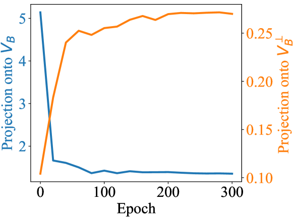
Figure 1: Projections of Squared Distance onto $V_{B}$ and $V_{B}^{\perp}$ show opposite trends as the training proceeds. The model is a ResNet50 trained on ImageNet-1K, using the setting specified in Section 6.1.

The proof of the proposition is provided in Appendix A.1. It is worth noting that the above proposition does not contradict previous conclusions that ETF configurations are the only minimizers (Zhu et al., 2021; Tirer & Bruna, 2022), since they require feature regularization $(\lambda_{H}/2)\|H\|_{F}^{2}$ in the loss function.

Our experiments show that Proposition 4.1 truly reflects the trend of neural network training. We train a ResNet50 model on ImageNet-1K dataset, and decompose $\Sigma_{W}$ into the $V_{B}$ part and the $V_{B}^{\perp}$ part by computing $(1/KN)\sum_{k\in[K],i\in[N]}\|\text{Proj}_{V_{B}}(h_{k,i}-\mu_{k})\|^{2}$ and $(1/KN)\sum_{k\in[K],i\in[N]}\|\text{Proj}_{V_{B}^{\perp}}(h_{k,i}-\mu_{k})\|^{2}$. The results are shown in Figure 1. We observe that although the $V_{B}$ part steadily decreases, the $V_{B}^{\perp}$ part keeps increasing in the training process. Therefore, $\Sigma_{W}\to\mathbf{0}$ may not occur for real world neural network training.

Proposition 4.1 and Figure 1 show that the last layer of neural networks exhibits high flexibility due to overparameterization. Consequently, it is unrealistic to expect standard empirical risk minimization training to achieve fully collapsed last layer representation, unless additional inductive bias are introduced. Therefore, requiring that the collapse metric reaches its minima only at fully collapsed configurations, such as Squared Distance, will be too stringent for practical use.

4.2 Invariance to Invertible Linear Transformations Matters

Symmetry and invariance is a core concept in deep learning (Gens & Domingos, 2014; Tan et al., 2018; Chen et al., 2019). The collapse metric discussed in Section 3.2 enjoy certain level of invariance properties.

Observation 4.2.

The Fuzziness metric $\operatorname{Tr}[\Sigma_{B}^{\dagger}\Sigma_{W}]$ is invariant to invertible linear transformation $U\in{\mathbb{R}}^{p\times p}$ that can be decomposed into two separate transformations in $V_{B}$ and $V_{B}^{\perp}$. The claim comes from the fact that

$$\quad\operatorname{Tr}\left[\left(U\Sigma_{B}U^{\top}\right)^{\dagger}U\Sigma_{W}U^{\top}\right]$$

$$=\operatorname{Tr}\left[U^{-1,\top}\Sigma_{B}^{\dagger}U^{-1}U\Sigma_{W}U^{\top}\right]$$

$$=\operatorname{Tr}\left[\Sigma_{B}^{\dagger}\Sigma_{W}\right].$$

However, Fuzziness is not invariant to all invertible linear transformations in ${\mathbb{R}}^{p}$. A simple counter example is $\Sigma_{B}=\left[\begin{array}[]{ll}1&0\\ 0&0\end{array}\right]$, $\Sigma_{W}=\left[\begin{array}[]{ll}1&0\\ 0&1\end{array}\right]$, and the linear transformation $U=\left[\begin{array}[]{ll}1&1\\ 0&1\end{array}\right]$. It can be calculated that $\operatorname{Tr}\left[\left(U\Sigma_{B}U^{\top}\right)^{\dagger}U\Sigma_{W}U^{\top}\right]=2\neq 1=\operatorname{Tr}\left[\Sigma_{B}^{\dagger}\Sigma_{W}\right]$.

Observation 4.3.

The Squared Distance metric in Equation 4 is invariant to isotropic scaling and orthogonal transformation on the feature vectors, i.e., since such transformations preserve the pairwise distance between the feature vectors. However, it is not invariant to invertible linear transformations in ${\mathbb{R}}^{p}$.

Observation 4.4.

The Cosine Similarity metric is invariant to independent scaling of each $h_{k,i}$. It is also invariant to orthogonal transformation in ${\mathbb{R}}^{p}$, as such transformations preserves the cosine similarity between feature vectors. But it is easy to see that Cosine Similarity is not invariant to invertible linear transformation in ${\mathbb{R}}^{p}$.

However, the next proposition shows that the linear probing loss of the last layer feature is invariant under a much more general class of transformations.

Observation 4.5.

The minimum value of loss function in Equation 4.1 is invariant to invertible linear transformations on the feature vector, i.e.

$$\min_{W,b}L(W,b,H)=\min_{W,b}L(W,b,VH),$$

for any invertible $V\in{\mathbb{R}}^{p\times p}$.

In other words, if we have two pretrained models $\phi_{1}(\cdot)$ and $\phi_{2}(\cdot)$, and there exists an invertible linear transformation $V\in{\mathbb{R}}^{p\times p}$ such that $\phi_{1}(x)=V\phi_{2}(x)$ for any $x\in{\mathbb{R}}^{d}$, then $\phi_{1}(\cdot)$ and $\phi_{2}(\cdot)$ will have exactly the same linear probing loss on any downstream data distribution. Therefore, when considering a collapse metric that may serve as an indicator of transfer accuracy, it is desirable for the metric to exhibit invariance to invertible linear transformations. However, as discussed previously, the metrics listed in Section 3.2 do not possess this level of invariance.

4.3 Numerical Stability Issues

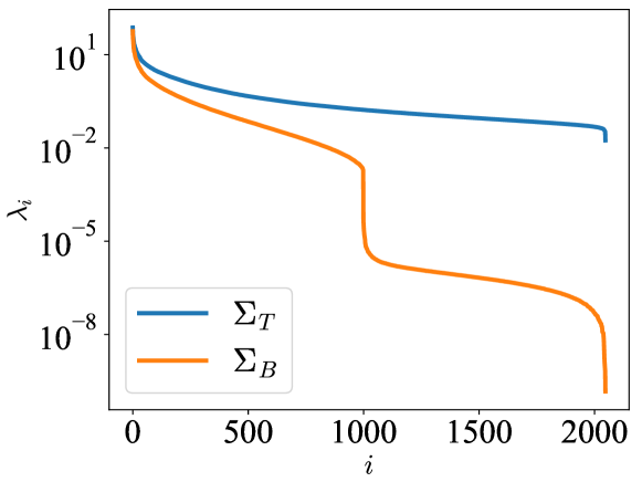
Figure 2: The Eigenvalue spectra of $\Sigma_{B}$ and $\Sigma_{T}$. The spectrum of $\Sigma_{T}$ has a substantially larger scale. The model is a ResNet50 trained on ImageNet-1K, using the setting specified in Section 6.1.

Numerical stability is an essential property for the collapse metric to ensure its practical usability. Unfortunately, the Fuzziness metric is prone to numerical instability, primarily due to the pseudoinverse operation applied to $\Sigma_{B}$.

Firstly, the between-class covariance matrix $\Sigma_{B}$ is singular when $K\leq p$, and its rank is unknown. Due to computational imprecision, its zero eigenvalues are always occupied with small nonzero values. In the default PyTorch (Paszke et al., 2019) implementation, the pseudoinverse operation includes a thresholding step to eliminate the spurious nonzero eigenvalues. However, selecting the appropriate threshold is a manual task, as it may vary depending on the architecture, dataset, or training algorithms.

To tackle this issue, one possible solution is to retain only the top $\min\{p,K-1\}$ eigenvalues, which is the maximum rank of $\Sigma_{B}$. Nevertheless, $\Sigma_{B}$ can still possess small trailing nonzero eigenvalues. For example, in the experiments illustrated in Figure 2, the $999$-th eigenvalue is about $2\times 10^{-3}$, significantly smaller than the typical scale of nonzero eigenvalues. Including such small eigenvalues in the computation would yield a substantially large fuzziness value.

To address the numerical stability issue, an alternative approach is to discard the $\Sigma_{B}$ and instead employ the more well-behaved overall covariance matrix $\Sigma_{T}$. As shown in Figure 2, the eigenvalues of $\Sigma_{T}$ exhibit a larger scale and a more uniform distribution compared with eigenvalues of $\Sigma_{B}$, making it a numerically stable choice for pseudoinverse operation. Interestingly, the quantity $\Sigma_{T}^{\dagger}$ naturally emerges in the solution of a loss minimization problem, which we will explore in the next section.

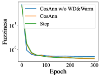
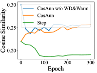
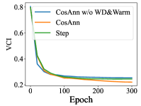
Figure 3: Variability Collapse metrics of training ResNet18 on CIFAR-10 dataset. From left to right: Fuzziness, Squared Distance, Cosine Similarity and our proposed VCI. The three curves are obtained with different training settings specified below, all achieving $\geq$ 92.1$\%$ test accuracy. Green: step-wise lerning rate decay schedule. Orange: cosine annealing schedule. Blue: cosine annealing schedule without weight decay and warmup.

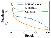
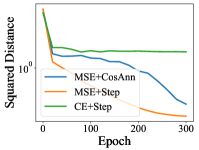
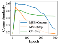
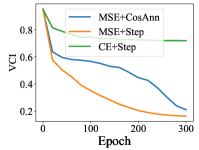
Figure 4: Variability Collapse metrics of training ResNet50 on ImageNet-1k dataset. From left to right: Fuzziness, Squared Distance, Cosine Similarity and our proposed VCI. The three curves are obtained with different training settings, all achieving $\geq$ 77.8$\%$ test accuracy. green: CE loss. orange: MSE loss. blue: MSE loss + cosine annealing schedule.

5 The Proposed Metric

As we have discussed, the existing collapse metrics discussed in Section 3.2 do not have the desired properties to fully measure the quality of the representation in downstream tasks. In this section, we introduce a novel and well-motivated collapse metric, which we call Variability Collapse Index (VCI), that satisfy all the aforementioned properties.

Previous studies (Zhu et al., 2021; Tirer & Bruna, 2022) indicate that fully collapsed last layer features minimizes the linear probing loss. Therefore, it is natural to explore the inverse direction, namely, using the linear probing loss to quantify the collapse level of last layer features.

Suppose we have a labeled dataset with corresponding last layer feature $H=(h_{k,i})_{k\in[K],i\in[N]}$. We perform linear regression on the last layer to find the optimal parameter $W$ that minimizes the following MSE loss:

$$L(W,b,H)=\frac{1}{2KN}\sum_{k\in[K],i\in[N]}\|Wh_{k,i}+b-e_{k}\|^{2}.$$

The following theorem gives the optimal linear probing loss.

Theorem 5.1.

The optimal linear probing loss has the following form.

$$\min_{W,b}L(W,b,H)=-\frac{1}{2K}\operatorname{Tr}\left[\Sigma_{T}^{\dagger}\Sigma_{B}\right]+\frac{1}{2}-\frac{1}{2K},$$

where $\Sigma_{B}$ and $\Sigma_{T}$ are the between-class and overall covariance matrix defined in Equation 2 and 3.

Theorem 5.1 shows that the information of the minimum MSE loss can be fully captured by the simple quantity $\operatorname{Tr}\left[\Sigma_{T}^{\dagger}\Sigma_{B}\right]$. It is easy to see that the minimum of $\operatorname{Tr}[\Sigma_{T}^{\dagger}\Sigma_{B}]$ is $0$. The following theorem gives an upper bound of $\operatorname{Tr}[\Sigma_{T}^{\dagger}\Sigma_{B}]$.

Theorem 5.2.

$\operatorname{Tr}[\Sigma_{T}^{\dagger}\Sigma_{B}]\leq\mathrm{rank}(\Sigma_{B})$. The equality holds for fully collapsed configuration $\Sigma_{W}=\mathbf{0}$.

The term $\operatorname{Tr}[\Sigma_{T}^{\dagger}\Sigma_{B}]$ has a positive correlation with the level of collapse in the representation. Theorem 5.1 implies that for MSE loss, a more collapsed representation leads to a smaller loss. Therefore, this term is a natural candidate for collapse metric.

Definition 5.3.

Define the Variability Collapse Index (VCI) of a set of features $H=(h_{k,i})_{k\in[K],i\in[N]}$ as

$$\text{VCI}=1-\frac{\operatorname{Tr}[\Sigma_{T}^{\dagger}\Sigma_{B}]}{\mathrm{rank}(\Sigma_{B})},$$

where $\Sigma_{B}$ and $\Sigma_{T}$ are the between-class and overall covariance matrix defined in Equation 2 and 3.

One of the advantages of VCI is its invariance to invertible linear transformations, which is inherited from the invariance of the MSE loss.

Corollary 5.4.

VCI is invariant to invertible linear transformation of the feature vector, i.e., multiplying each $h_{k,i}$ with an invertible matrix $U\in{\mathbb{R}}^{p\times p}$.

Proof.

From Observation 4.5, we know that the minimum of the loss function $L(W,b,H)$ is invariant to invertible linear transformations on $H$. This implies the same invariance property of the term $\operatorname{Tr}[\Sigma_{T}^{\dagger}\Sigma_{B}]$. The proof is complete by noting that invertible linear transformation will also preserve the rank of $\Sigma_{B}$. ∎

Another advantage of VCI lies in its numerical stability. This advantage primarily stems from the well-behaved nature of the spectrum of $\Sigma_{T}$ compared to that of $\Sigma_{B}$, as discussed in Section 4.3. Therefore, the pseudo-inverse operation does not lead to an explosive increase in VCI. Furthermore, one can safely takes $\mathrm{rank}(\Sigma_{B})=\min\{p,K-1\}$, since the unknown rank is not the cause of numerically instability as in Fuziness.

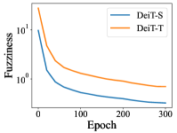
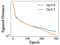
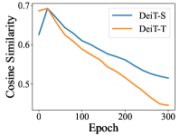
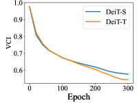
Figure 5: Variability Collapse metrics of training ViT on ImageNet-1k dataset. From left to right: Fuzziness, Squared Distance, Cosine Similarity and our proposed VCI. Blue: DeiT-S. Orange: DeiT-T. All of the four metrics indicate variability collapse happens for this setting.

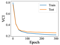
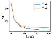
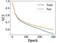
Figure 6: Train Collapse and Test Collapse both happen for VCI. Train collapse is evaluated on a 50000 subset of ImageNet-1K training dataset. Test collapse is evaluated on the full ImageNet-1K test dataset. Left: ResNet18 on CIFAR-10. Middle: ResNet50 on ImageNet-1K. Right: DeiT-S on ImageNet-1K.

6 Experiment Results

In this section, we present experiments that reflect the differences between the previous variability collapse metrics and our proposed VCI metric.

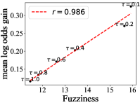
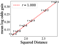
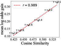
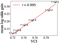
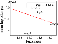
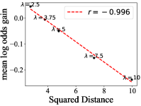
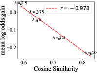
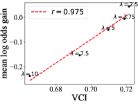
Figure 7: Only VCI consistently indicates transferability in both groups of our experiments: In each graph, x-axis represents the metric value evaluated on a 50000 subset of ImageNet train set, y-axis shows the mean log odds gain defined as in Equation 6, and the Pearson correlation coefficient is shown in the legend. Top Row: A negative relation between all variability metrics and transferability can be observed when changing the temperature $\tau$ of softmax in pretraining. Bottom Row: Nearly opposite trends emerge on previous variability metrics when we adjust the coefficient $\lambda$ of the Cosine Similarity regularization term. In contrast, VCI maintains a positive correlation with the mean log odds gain.

6.1 Setups

We conduct experiments to analyze the behavior of four variability collapse metrics, namely Fuzziness, Squared Distance, Cosine Similarity. We evaluate the metrics on the feature layer of ResNet18 (He et al., 2016) trained on CIFAR10 (Krizhevsky et al., 2009) and ResNet50 / variants of ViT (Dosovitskiy et al., 2020) trained on ImageNet-1K with AutoAugment (Cubuk et al., 2018) for 300 epochs. ResNet18s are trained on one NVIDIA GeForce RTX 3090 GPU, ResNet50s and ViT variants are trained on four GPUs. The batchsize for each GPU is set to 256. The metric values are recorded every 20 epochs, where $\operatorname{rank}(\Sigma_{B})$ in the expression of VCI is taken to be $\min\{p,K-1\}$ as stated in the previous section.

For all experiments on ResNet models, We use the implementation of ResNet from the torchvision library, called ‘ResNet v1.5’. We use SGD with Nesterov Momentum as the optimizer. The maximum learning rate is set to $0.1\times\text{batch size}/256$. We try both the cosine annealing and step-wise learning rate decay scheduler. When using a step-wise learning rate decay schedule, the learning rate is decayed by a factor of 0.975 every epoch. We also use a linear warmpup procedure of 10 epochs, starting from an initial $10^{-5}$ learning rate. The weight-decay factor is set to $8\times 10^{-5}$. For training on CIFAR10, we replace the random resized crop with random crop after padding 4 pixels on each side as in He et al. (2016). Cross-Entropy loss is used if not specified otherwise.

For DeiT-T and DeitT-S (Touvron et al., 2021a), the two ViT variants used in our experiments, we use AdamW (Loshchilov & Hutter, 2017) with a cosine annealing scheduler as the optimizer. We incorporate a linear warm-up phase of 5 epochs, starting from a learning rate of $10^{-6}$ and gradually increasing to the maximum learning rate of $10^{-3}$. For other modules of training, such as weight initialization, mixup/cutmix, stochastic depth and random erasing, we keep the same with those of Touvron et al. (2021a).

At test time for ImageNet-1K, we resize the short side of image to a length of 256 pixels and perform a center crop. When evaluating the variability collapse metrics, we use the same data transformation as at test time. All transformed images are finally normalized with ImageNet mean and standard deviation during training, testing, and metric evaluation.

6.2 How do Variability Collapse Metrics Evolve as the Training Proceeds

Figure 3 demonstrates the trend of four different variability collapse metrics when training ResNet18 on CIFAR-10. It is observed that Squared Distance and Cosine Similarity fail to exhibit a consistent trend of collapse, as explained in Section 4.1. On the other hand, Fuzziness and VCI show a decreasing trend across these settings.

The results for ResNet50s trained on ImageNet are provided in Figure 4. In contrast to the case of ResNet18 on CIFAR10, all evaluated metrics consistently demonstrate a decreasing curve since the ratio of the $V_{B}^{\perp}$ part becomes smaller with a smaller $p/K$ value, as shown in Figure 1. Additionally, it is observed that neural networks trained with MSE loss exhibit a higher level of collapse compared to those trained with CE loss, which aligns with the findings of Kornblith et al. (2021).

The results for ViT variants trained on ImageNet are given in Figure 5. For DeiT-T and DeitT-S with embedding dimensions of 192 and 384, $V_{B}$ becomes the whole feature space due to $p<K$, leading to a clearer trend of variability collapse since $V_{B}^{\perp}$ becomes $0$.

Finally, we show that test collapse also happens for VCI in Figure 6. This indicates that variability collapse is a phenomenon that reflects the properties of underlying data distributions, rather than being solely caused by overfitting the training datasets. We refer to Appendix B for comparisons between train collapse and test collapse for other variability metrics.

6.3 Only VCI consistently Indicates Transferability

In this section, we investigate the correlation between variability metrics and transferability through two sets of experiments. We pretrain ResNet50 on ImageNet-1K with a single varying hyperparameter specified within each group. We evaluate the pretrained neural representations using linear probing (Kornblith et al., 2019; Chen et al., 2020) on 10 downstream datasets, including Oxford-IIIT Pets (Parkhi et al., 2012), Oxford 102 Flowers (Nilsback & Zisserman, 2008), FGVC Aircraft (Maji et al., 2013), Stanford Cars (Krause et al., 2013), the Describable Textures Dataset (DTD) (Cimpoi et al., 2014), Food-101 dataset (Bossard et al., 2014), CIFAR-10 and CIFAR-100 (Krizhevsky et al., 2009), Caltech-101 (L. Fei-Fei et al., 2004), the SUN397 scene dataset (Xiao et al., 2010). We use L-BFGS to train the linear classifier, with the optimal $L_{2}$-penalty strength determined by searching through 97 logarithmically spaced values between $10^{-6}$ and $10^{6}$ on a validation set. We provide the raw experiment results in Appendix C.

We use the following mean log odds gain

$$\operatorname{MLOG}=\frac{1}{10}\sum_{i=1}^{10}\log\frac{p_{i}}{1-p_{i}}-\log\frac{p_{\text{pretrain}}}{1-p_{\text{pretrain}}}$$ (6)

to measure the transferability of a neural representation, where $p_{\text{pretrain}}$ is the final test accuracy in pretraining. Compared with Kornblith et al. (2019), we subtract the log odds of the pretrain accuracy from the mean log odds of linear classification accuracy over the downstream tasks, to isolate the impact of variability collapse on transfer performance.

In the first group, we change the temperature $\tau$ in the softmax function

$$\operatorname{Softmax}_{\tau}(z)=\left(\frac{\exp(\frac{1}{\tau}z_{1})}{\sum_{k=1}^{K}\exp(\frac{1}{\tau}z_{k})},\cdots,\frac{\exp(\frac{1}{\tau}z_{K})}{\sum_{k=1}^{K}\exp(\frac{1}{\tau}z_{k})}\right).$$

The results of the first group of experiments are shown in the top row of Figure 7. The results are consistent with the findings in (Kornblith et al., 2021), as all considered metrics show a negative relation between variability collapse and transfer performance.

In the second group of experiments, we introduce regularization to control the collapse behavior of neural networks (Kornblith et al., 2021). The regularization term we used is the average within-class cosine similarity divided by the number of data points of each class in the batch. By varying the value of $\lambda$ multiplied to the regularization term, we investigate whether the observed correlation in the first group still holds true. The bottom row of Figure 7 shows that for the three previous metrics, the correlation changes from positive to negative, or vice versa. However, a strong positive correlation consistently holds between VCI and transferability. Therefore, VCI serves as an effective indicator of transfer performance, compared to other variability collapse metrics.

7 Conclusions and Future Directions

In this paper, we study the variability collapse phenomenon of neural networks, and propose the VCI metric as a quantitative characterization. We demonstrate that VCI enjoys many desired properties, including invariance and numerical stability, and verify its usefulness via extensive experiments.

Moving forward, there are several promising directions for future research. Firstly, it would be beneficial to explore the applicability of VCI to a broader range of training recipes and architectures, by analyzing its performance using alternative network architectures, training methodologies, and datasets. Secondly , it would be valuable to conduct theoretical investigations into the relationship between variability collapse and transfer accuracy. Understanding the mechanisms and principles behind this could provide insights to designing better transfer learning algorithms.

Appendix A Proofs

A.1 Proof of Proposition 4.1

Proof.

Since $p>K$, we can find a nonzero vector $v\in{\mathbb{R}}^{p}$, such that $Wv=\mathbf{0}$. For some $\lambda>0$, define the elements of $H^{\prime}$ as

$$h_{k,i}^{\prime}=\begin{cases}h_{k,i}+\lambda v&i=1,\\ h_{k,i}&2\leq i\leq N.\end{cases}$$

For such an $H^{\prime}$, we have $Wh_{k,i}=Wh_{k,i}^{\prime}$, and therefore $L(W,b,H)=L(W,b,H^{\prime})$. Furthermore, we can calculate $\mu_{k}(H^{\prime})=\mu_{k}(H)+\frac{\lambda}{N}v$, and $\mu_{G}(H^{\prime})=\mu_{G}(H)+\frac{\lambda}{N}v$, which implies that $\Sigma_{B}(H^{\prime})=\Sigma_{B}(H)$.

Next, we calculate $\Sigma_{W}(H^{\prime})$:

$$\Sigma_{W}(H^{\prime}) =\frac{1}{KN}\sum_{k\in[K],i\in[N]}\left(h_{k,i}^{\prime}-\mu_{k}(H^{\prime})\right)\left(h_{k,i}^{\prime}-\mu_{k}(H^{\prime})\right)^{\top}$$

$$=\frac{1}{KN}\sum_{k=1}^{K}\left[\left(h_{k,1}+\lambda v-\mu_{k}(H)-\frac{\lambda}{N}v\right)\left(h_{k,1}+\lambda v-\mu_{k}(H)-\frac{\lambda}{N}v\right)^{\top}\right.$$

$$\left.\quad+\sum_{i=2}^{N}\left(h_{k,i}-\mu_{k}(H)-\frac{\lambda}{N}v\right)\left(h_{k,i}-\mu_{k}(H)-\frac{\lambda}{N}v\right)^{\top}\right]$$

$$=\frac{1}{KN}\sum_{k=1}^{K}\left[\left(h_{k,1}-\mu_{k}(H)\right)\left(h_{k,1}-\mu_{k}(H)\right)^{\top}+\frac{\lambda(N-1)}{N}v(h_{k,1}-\mu_{k}(H))^{\top}\right.$$

$$\left.\quad+\frac{\lambda(N-1)}{N}(h_{k,1}-\mu_{k}(H))v^{\top}+\frac{\lambda^{2}(N-1)^{2}}{N^{2}}vv^{\top}+\sum_{i=2}^{N}\left(h_{k,i}-\mu_{k}(H)\right)\left(h_{k,i}-\mu_{k}(H)\right)^{\top}\right.$$

$$\left.\quad-\frac{\lambda}{N}v\sum_{i=2}^{N}\left(h_{k,i}-\mu_{k}(H)\right)^{\top}-\frac{\lambda}{N}\sum_{i=2}^{N}\left(h_{k,i}-\mu_{k}(H)\right)v^{\top}+\frac{\lambda^{2}(N-1)}{N^{2}}vv^{\top}\right]$$

$$=\frac{1}{KN}\sum_{k=1}^{K}\left[\sum_{i=1}^{N}\left(h_{k,i}-\mu_{k}(H)\right)\left(h_{k,i}-\mu_{k}(H)\right)^{\top}+\frac{\lambda}{N}v\left((N-1)h_{k,1}-\sum_{i=2}^{N}h_{k,i}\right)^{\top}\right.$$

$$\left.\quad+\frac{\lambda}{N}\left((N-1)h_{k,1}-\sum_{i=2}^{N}h_{k,i}\right)v^{\top}+\frac{\lambda^{2}(N-1)}{N}vv^{\top}\right]$$

$$=\Sigma_{W}(H)+\frac{\lambda}{KN^{2}}\left[v\sum_{k=1}^{K}\left((N-1)h_{k,1}-\sum_{i=2}^{N}h_{k,i}\right)^{\top}\right.$$

$$\left.\quad+\sum_{k=1}^{K}\left((N-1)h_{k,1}-\sum_{i=2}^{N}h_{k,i}\right)v^{\top}\right]+\frac{\lambda^{2}(N-1)}{N^{2}}vv^{\top}.$$

Since $VV^{\top}$ is a nonzero positive semidefinite matrix, we can let $\lambda\to\infty$ and get $\|\Sigma_{W}(H^{\prime})\|_{F}\to\infty$. ∎

A.2 Proof of Theorem 5.1

Proof.

Without loss of generality, we can assume that $\mu_{G}=0$, since we can replace $b$ with $b-W\mu_{G}$. The loss contributed by the $i$-th datapoint in the $k$-th class can be calculated as

$$L_{k,i}(W,b) \triangleq\frac{1}{2}\|Wh_{k,i}+b-e_{k}\|^{2}$$

$$=\frac{1}{2}\left[h_{k,i}^{\top}W^{\top}Wh_{k,i}+2(b-e_{k})^{\top}Wh_{k,i}+(b-e_{k})^{\top}(b-e_{k})\right]$$

$$=\frac{1}{2}\operatorname{Tr}\left[h_{k,i}h_{k,i}^{\top}W^{\top}W\right]+b^{\top}Wh_{k,i}-e_{k}^{\top}Wh_{k,i}+\frac{1}{2}b^{\top}b-e_{k}^{\top}b+\frac{1}{2}.$$

The total loss function can be calculated as

$$L(W,b) =\frac{1}{KN}\sum_{k\in[K],i\in[N]}L_{k,i}(W,b)$$

$$=\frac{1}{2}\operatorname{Tr}\left[\Sigma_{T}W^{\top}W\right]-\frac{1}{K}\sum_{k=1}^{K}e_{k}^{\top}W\mu_{k}+\frac{1}{2}b^{\top}b-\frac{1}{K}\mathbf{1}^{\top}b+\frac{1}{2}.$$

The loss function is convex and quadratic, whose optima can be obtained by first order stationary condition. The first order condition with regard to $W$ can be expressed as

$$\nabla_{W}L(W,b)=W\Sigma_{T}-\frac{1}{K}\sum_{k=1}^{K}e_{k}\mu_{k}^{\top}=0.$$

To solve this equality, we make a little digress and prove the following bias-variance decomposition:

$$\begin{aligned} \Sigma_{T}&=\frac{1}{KN}\sum_{k\in[K],i\in[N]}h_{k,i}h_{k,i}^{\top}\\ &=\frac{1}{KN}\sum_{k\in[K],i\in[N]}(h_{k,i}-\mu_{k}+\mu_{k})(h_{k,i}-\mu_{k}+\mu_{k})^{\top}\\ &=\frac{1}{KN}\sum_{k\in[K],i\in[N]}(h_{k,i}-\mu_{k})(h_{k,i}-\mu_{k})^{\top}+\frac{2}{KN}\sum_{k\in[K],i\in[N]}(h_{k,i}-\mu_{k})\mu_{k}^{\top}+\frac{1}{K}\sum_{k\in[K]}\mu_{k}\mu_{k}^{\top}\\ &=\Sigma_{B}+\Sigma_{W},\end{aligned}$$ (7)

From this we know that $\Sigma_{T}-\Sigma_{B}=\Sigma_{W}$ is positive semidefinite. This implies that $\mu_{1},\cdots,\mu_{k}$ lies in the column space $V_{T}$ of $\Sigma_{T}$.

Let $r=\text{rank}(\Sigma_{T})$. There exists a eigenvalue decomposition $\Sigma_{T}=U\Sigma U^{\top}$, such that $\Sigma=\text{diag}(s_{1},\cdots s_{r},0,\cdots,0)$, and $U=(u_{1},\cdots u_{d})$ satisfying

$$1.\;\ u_{i}\perp u_{j},\ i\neq j;\quad 2.\;\|u_{i}\|_{2}=1;\quad 3.\;u_{i}\perp\mu_{k},\ k\leq K,i>K.$$

Therefore

$$\frac{1}{K}\left(\sum_{k=1}^{K}e_{k}\mu_{k}^{\top}\right)\Sigma_{T}^{\dagger}\Sigma_{T} =\frac{1}{K}\left(\sum_{k=1}^{K}e_{k}\mu_{k}^{\top}\right)U\Sigma^{\dagger}U^{\top}U\Sigma U^{\top}$$

$$=\frac{1}{K}\left(\sum_{k=1}^{K}e_{k}\mu_{k}^{\top}\right)\cdot\left(\sum_{i=1}^{r}u_{i}u_{i}^{\top}\right)$$

$$=\frac{1}{K}\left(\sum_{k=1}^{K}e_{k}\mu_{k}^{\top}\right)-\frac{1}{K}\left(\sum_{k=1}^{K}e_{k}\mu_{k}^{\top}\right)\cdot\left(\sum_{i=r+1}^{d}u_{i}u_{i}^{\top}\right)$$

$$=\frac{1}{K}\left(\sum_{k=1}^{K}e_{k}\mu_{k}^{\top}\right).$$

This implies that $W=\frac{1}{K}\left(\sum_{k=1}^{K}e_{k}\mu_{k}^{\top}\right)\Sigma_{T}^{\dagger}$ satisfies the first order optimality condition for $W$. It is also easy to see that $b=\frac{1}{K}\mathbf{1}$ satisfies the first order optimality condition of $b$. Therefore, $L(W,b)$ attains its minimum at

$$W=\frac{1}{K}\left(\sum_{k=1}^{K}e_{k}\mu_{k}^{\top}\right)\Sigma_{T}^{\dagger},\quad b=\frac{1}{K}\mathbf{1},$$

with optimal value

$$\min_{W,b}L(W,b) =\frac{1}{2}\operatorname{Tr}\left[\Sigma_{T}\cdot\Sigma_{T}^{\dagger}\cdot\frac{1}{K}\left(\sum_{k=1}^{K}\mu_{k}e_{k}^{\top}\right)\cdot\frac{1}{K}\left(\sum_{k=1}^{K}e_{k}\mu_{k}^{\top}\right)\Sigma_{T}^{\dagger}\right]$$

$$\quad-\operatorname{Tr}\left[\frac{1}{K}\left(\sum_{k=1}^{K}\mu_{k}e_{k}^{\top}\right)\cdot\frac{1}{K}\left(\sum_{k=1}^{K}e_{k}\mu_{k}^{\top}\right)\Sigma_{T}^{\dagger}\right]+\frac{1}{2}-\frac{1}{2K}$$

$$=-\frac{1}{2K}\operatorname{Tr}\left[\frac{1}{K}\left(\sum_{k=1}^{K}\mu_{k}\mu_{k}^{\top}\right)\cdot\Sigma_{T}^{\dagger}\right]+\frac{1}{2}-\frac{1}{2K}$$

$$=-\frac{1}{2K}\operatorname{Tr}\left[\Sigma_{T}^{\dagger}\Sigma_{B}\right]+\frac{1}{2}-\frac{1}{2K}$$

where we use $\Sigma_{T}^{\dagger}\Sigma_{T}\Sigma_{T}^{\dagger}=\Sigma_{T}^{\dagger}$ in the second equality. ∎

A.3 Proof for Theorem 5.2

We need the following lemmas on block matrices.

Lemma A.1.

Let $A\in{\mathbb{R}}^{d_{1}\times d_{1}},B\in{\mathbb{R}}^{d_{1}\times d_{2}},C\in{\mathbb{R}}^{d_{2}\times d_{1}},D\in{\mathbb{R}}^{d_{2}\times d_{2}}$. If $\left[\begin{array}[]{ll}{A}&{B}\\ {C}&{D}\end{array}\right]$ and $D$ are invertible, then ${A}-{BD}^{-1}{C}$ is invertible and

$$\left[\begin{array}[]{ll}{A}&{B}\\ {C}&{D}\end{array}\right]^{-1}=\left[\begin{array}[]{cc}\left({A}-{BD}^{-1}{C}\right)^{-1}&-\left({A}-{BD}^{-1}{C}\right)^{-1}{BD}^{-1}\\ -{D}^{-1}{C}\left({A}-{BD}^{-1}{C}\right)^{-1}&{D}^{-1}+{D}^{-1}{C}\left({A}-{BD}^{-1}{C}\right)^{-1}{BD}^{-1}\end{array}\right].$$ (12)

Proof.

The invertibility of $A$ and $D$ are obvious. The following identity gives the invertibility of ${A}-{BD}^{-1}{C}$:

$$\left[\begin{array}[]{cc}A&B\\ C&D\end{array}\right]\left[\begin{array}[]{cc}\mathbf{I}&\mathbf{0}\\ -D^{-1}C&\mathbf{I}\end{array}\right]=\left[\begin{array}[]{cc}A-BD^{-1}C&B\\ \mathbf{0}&D\end{array}\right]$$

The equation 12 can be check by direct calculation.

∎

Lemma A.2.

Let $A\in{\mathbb{R}}^{d_{1}\times d_{1}},B\in{\mathbb{R}}^{d_{1}\times d_{2}},C\in{\mathbb{R}}^{d_{2}\times d_{2}}$. If $\left[\begin{array}[]{ll}{A}&{B}\\ {B}^{\top}&{C}\end{array}\right]\succ\mathbf{0}$, then ${A}-{BC}^{-1}{B}^{\top}\succ\mathbf{0}$.

Proof.

It is the direct consequence of the following identity.

$$\begin{aligned} &\left(\begin{array}[]{cc}\mathbf{I}&\mathbf{0}\\ -B^{\top}A^{-1}&\mathbf{I}\end{array}\right)\left(\begin{array}[]{cc}A&B\\ B^{\top}&C\end{array}\right)\left(\begin{array}[]{cc}\mathbf{I}&\mathbf{0}\\ -B^{\top}A^{-1}&\mathbf{I}\end{array}\right)^{\top}=\left(\begin{array}[]{cc}A&\mathbf{0}\\ \mathbf{0}&C-B^{\top}A^{-1}B\end{array}\right)\end{aligned}$$

∎

Proof of Theorem 5.2.

Let $r=\mathrm{rank}(\Sigma_{T})$. There exists an eigenvalue decomposition $\Sigma_{T}=U\left[\begin{array}[]{ll}\Sigma&\\ &\mathbf{0}\end{array}\right]U^{\top}$ with $\Sigma=\text{diag}(s_{1},\cdots s_{r})$. From Equation 7, we know that $V_{B}$, the column space of $\Sigma_{B}$ is a subspace of $V_{T}$, the column space of $\Sigma_{T}$. Therefore, there exists $W\in{\mathbb{R}}^{r\times r}$, such that $\Sigma_{B}=U\left[\begin{array}[]{ll}W&\\ &\mathbf{0}\end{array}\right]U^{\top}$. This implies that

$$\operatorname{Tr}\left[\Sigma_{T}^{\dagger}\Sigma_{B}\right] =\operatorname{Tr}\left[(U\left[\begin{array}[]{ll}\Sigma&\\ &\mathbf{0}\end{array}\right]U^{\top})^{\dagger}U\left[\begin{array}[]{ll}W&\\ &\mathbf{0}\end{array}\right]U^{\top}\right]$$

$$=\operatorname{Tr}\left[U\left[\begin{array}[]{ll}\Sigma&\\ &\mathbf{0}\end{array}\right]^{\dagger}U^{\top}U\left[\begin{array}[]{ll}W&\\ &\mathbf{0}\end{array}\right]U^{\top}\right]$$

$$=\operatorname{Tr}[\Sigma^{-1}W]$$

Let $r_{1}=\mathrm{rank}(W)$. Denote $W=U_{1}\left[\begin{array}[]{ll}\Sigma_{1}&\\ &\mathbf{0}\end{array}\right]U_{1}^{\top}$ as the eigenvalue decomposition of $W$. Denote $V=\left[\begin{array}[]{ll}V_{1}&V_{2}\\ V_{2}^{\top}&V_{3}\end{array}\right]=U_{1}^{\top}\Sigma U_{1}$, where $V_{1}\in{\mathbb{R}}^{r_{1}\times r_{1}}$. Since $V\succ\mathbf{0}$, we can evoke Lemma A.1 have

$$\operatorname{Tr}\left[\Sigma^{-1}W\right] =\operatorname{Tr}\left[U_{1}V^{-1}U_{1}^{\top}U_{1}\left[\begin{array}[]{ll}\Sigma_{1}&\\ &\mathbf{0}\end{array}\right]U_{1}^{\top}\right]$$

$$=\operatorname{Tr}\left[\left(V_{1}-V_{2}^{\top}V_{3}^{-1}V_{2}\right)^{-1}\Sigma_{1}\right]$$

From Equation 7, we know that $W\preceq\Sigma$. Use Lemma A.2, we get $\mathbf{0}\prec\Sigma_{1}\preceq V_{1}-V_{2}^{\top}V_{3}^{-1}V_{2}$. This implies that

$$\operatorname{Tr}\left[\left(V_{1}-V_{2}^{\top}V_{3}^{-1}V_{2}\right)^{-1}\Sigma_{1}\right] =r_{1}-\operatorname{Tr}\left[\left(V_{1}-V_{2}^{\top}V_{3}^{-1}V_{2}\right)^{-1}\left(V_{1}-V_{2}^{\top}V_{3}^{-1}V_{2}-\Sigma_{1}\right)\right]\leq r_{1},$$

where in the last inequality, we use the fact that the trace of the product of two symmetric positive semidefinite matrices is nonnegative. Therefore, we obtain the inequality that

$$\operatorname{Tr}[\Sigma_{T}^{\dagger}\Sigma_{B}]\leq\mathrm{rank}(\Sigma_{B}).$$

For fully collapsed configuration, we have $\Sigma_{B}=\Sigma_{T}$, and the equality is attained.

∎

Appendix B Additional Experimental Results in Section 6.2

We show in Figure 8 the test collapse for Fuzziness, Squared Distance and Cosine Similarity.

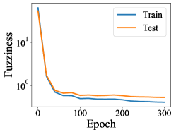
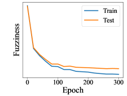
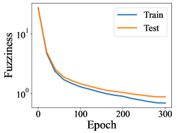
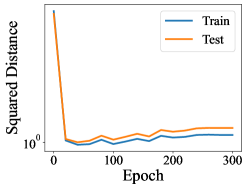
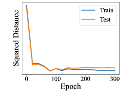
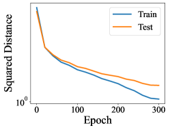
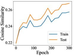
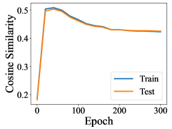
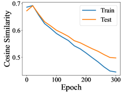
Figure 8: Additional Experiments on the Comparisons of Train Collapse and Test Collapse for Previous Variability Collapse Metrics. Train collapse is evaluated on a 50000 subset of ImageNet-1K training dataset. Top Row: Fuzziness. Middle Row: Squared Distance. Bottom Row: Cosine Similarity. Left: ResNet18 on CIFAR-10. Middle: ResNet50 on ImageNet-1K. Orange: DeiT-S on ImageNet-1K.

Appendix C Raw Experiment Data in Section 6.3

See Table 1 and Table 2 for raw data in downstread classification experiments and pretraining experiments, respectively. For Aircraft, Pets, Caltech101 and Flowers, we use mean per-class accuracy. (Chen et al., 2020) For other datasets, we use top-1 accuracy.

Table 1: Raw data of downstream classification experiments in Section 6.3. The meanings of $\tau$ and $\lambda$ are introduced in the main text. MLO = mean log odds.

Param	Pets	Flowers	Aircraft	Cars	DTD	Cifar10	Food101	Cifar100	Caltech	SUN397	MLO
$\tau=0.1$	90.8	95.03	58.85	64.73	74.47	93.1	75.45	77.14	84.9	62.44	1.445
$\tau=0.2$	91.52	95.25	57.5	64.1	74.41	92.89	75.41	77.65	85.58	63.28	1.459
$\tau=0.4$	91.64	94.66	57.67	64.42	74.63	92.58	74.97	77.1	85.59	63.3	1.441
$\tau=0.6$	91.74	94.14	57.54	61.56	76.22	92.42	74.86	76.6	85.2	63.51	1.421
$\tau=0.8$	92.35	93.52	55.64	61.6	75.37	92.37	74.2	76.07	84.49	62.74	1.39
$\tau=1.0$	91.7	93.68	55.37	60.14	73.99	91.9	74.42	75.96	85.82	62.98	1.375
$\lambda=2.5$	90.86	92.01	51.07	55.14	74.36	91.79	72.9	75.44	85.19	62.01	1.282
$\lambda=3.75$	90.87	90.79	47.81	50.44	76.01	91.89	72.19	75.31	82.97	60.98	1.22
$\lambda=5$	90.51	90.03	45.12	50.52	74.41	91.63	71.84	74.64	82.63	60.38	1.174
$\lambda=7.5$	89.33	86.54	44.52	46.87	73.14	91.64	71.19	74.13	81.23	58.55	1.08
$\lambda=10$	89.92	83.6	43.39	43.55	72.5	91.43	70.29	73.76	78.25	56.9	1.008

Table 2: Raw data of pretraining runs in Section 6.3.

Param	Fuzziness	Sqr Dist	Cos Sim	VCI	Accuracy	MLOG
$\tau=0.1$	15.93	2.829	0.4634	0.796	75.4	0.3250
$\tau=0.2$	15.64	2.534	0.4856	0.7849	76.64	0.2704
$\tau=0.4$	13.45	2.141	0.512	0.7552	77.53	0.2029
$\tau=0.6$	12.62	1.923	0.5371	0.7406	77.72	0.1711
$\tau=0.8$	11.83	1.742	0.5589	0.728	77.83	0.1343
$\tau=1.0$	11.46	1.625	0.5767	0.7201	77.88	0.1161
$\lambda=2.5$	13.15	2.78	0.4097	0.7216	77.52	0.0440
$\lambda=3.75$	14.31	3.803	0.3556	0.719	77.31	-0.0063
$\lambda=5$	14.51	4.783	0.3551	0.7099	77.29	-0.0507
$\lambda=7.5$	15.22	7.287	0.2794	0.6936	77.46	-0.1539
$\lambda=10$	13.92	9.964	0.172	0.6652	77.65	-0.2375

References

- Abnar et al. (2021) Abnar, S., Dehghani, M., Neyshabur, B., and Sedghi, H. Exploring the limits of large scale pre-training. arXiv preprint arXiv:2110.02095, 2021.
- Baevski et al. (2022) Baevski, A., Hsu, W.-N., Xu, Q., Babu, A., Gu, J., and Auli, M. Data2vec: A general framework for self-supervised learning in speech, vision and language. arXiv preprint arXiv:2202.03555, 2022.
- Bommasani et al. (2021) Bommasani, R., Hudson, D. A., Adeli, E., Altman, R., Arora, S., von Arx, S., Bernstein, M. S., Bohg, J., Bosselut, A., Brunskill, E., et al. On the opportunities and risks of foundation models. arXiv preprint arXiv:2108.07258, 2021.
- Bossard et al. (2014) Bossard, L., Guillaumin, M., and Van Gool, L. Food-101–mining discriminative components with random forests. In Computer Vision–ECCV 2014: 13th European Conference, Zurich, Switzerland, September 6-12, 2014, Proceedings, Part VI 13, pp. 446–461. Springer, 2014.
- Chen et al. (2022) Chen, M., Fu, D. Y., Narayan, A., Zhang, M., Song, Z., Fatahalian, K., and Ré, C. Perfectly balanced: Improving transfer and robustness of supervised contrastive learning. In International Conference on Machine Learning, pp. 3090–3122. PMLR, 2022.
- Chen et al. (2019) Chen, S., Dobriban, E., and Lee, J. H. Invariance reduces variance: Understanding data augmentation in deep learning and beyond. arXiv preprint arXiv:1907.10905, 2019.
- Chen et al. (2020) Chen, T., Kornblith, S., Norouzi, M., and Hinton, G. A simple framework for contrastive learning of visual representations. In International conference on machine learning, pp. 1597–1607. PMLR, 2020.
- Cimpoi et al. (2014) Cimpoi, M., Maji, S., Kokkinos, I., Mohamed, S., and Vedaldi, A. Describing textures in the wild. In Proceedings of the IEEE conference on computer vision and pattern recognition, pp. 3606–3613, 2014.
- Cubuk et al. (2018) Cubuk, E. D., Zoph, B., Mane, D., Vasudevan, V., and Le, Q. V. Autoaugment: Learning augmentation policies from data. arXiv preprint arXiv:1805.09501, 2018.
- Cui et al. (2022) Cui, Q., Zhao, B., Chen, Z.-M., Zhao, B., Song, R., Zhou, B., Liang, J., and Yoshie, O. Discriminability-transferability trade-off: an information-theoretic perspective. In Computer Vision–ECCV 2022: 17th European Conference, Tel Aviv, Israel, October 23–27, 2022, Proceedings, Part XXVI, pp. 20–37. Springer, 2022.
- Dosovitskiy et al. (2020) Dosovitskiy, A., Beyer, L., Kolesnikov, A., Weissenborn, D., Zhai, X., Unterthiner, T., Dehghani, M., Minderer, M., Heigold, G., Gelly, S., et al. An image is worth 16x16 words: Transformers for image recognition at scale. arXiv preprint arXiv:2010.11929, 2020.
- Dubois et al. (2022) Dubois, Y., Ermon, S., Hashimoto, T. B., and Liang, P. S. Improving self-supervised learning by characterizing idealized representations. Advances in Neural Information Processing Systems, 35:11279–11296, 2022.
- Fang et al. (2023) Fang, A., Kornblith, S., and Schmidt, L. Does progress on imagenet transfer to real-world datasets? arXiv preprint arXiv:2301.04644, 2023.
- Fang et al. (2021) Fang, C., He, H., Long, Q., and Su, W. J. Exploring deep neural networks via layer-peeled model: Minority collapse in imbalanced training. Proceedings of the National Academy of Sciences, 118(43):e2103091118, 2021.
- Feng et al. (2021) Feng, Y., Jiang, J., Tang, M., Jin, R., and Gao, Y. Rethinking supervised pre-training for better downstream transferring. arXiv preprint arXiv:2110.06014, 2021.
- Galanti et al. (2021) Galanti, T., György, A., and Hutter, M. On the role of neural collapse in transfer learning. arXiv preprint arXiv:2112.15121, 2021.
- Gens & Domingos (2014) Gens, R. and Domingos, P. M. Deep symmetry networks. Advances in neural information processing systems, 27, 2014.
- Grill et al. (2020) Grill, J.-B., Strub, F., Altché, F., Tallec, C., Richemond, P., Buchatskaya, E., Doersch, C., Avila Pires, B., Guo, Z., Gheshlaghi Azar, M., et al. Bootstrap your own latent-a new approach to self-supervised learning. Advances in neural information processing systems, 33:21271–21284, 2020.
- Han et al. (2021) Han, X., Papyan, V., and Donoho, D. L. Neural collapse under mse loss: Proximity to and dynamics on the central path. arXiv preprint arXiv:2106.02073, 2021.
- He & Su (2022) He, H. and Su, W. J. A law of data separation in deep learning. arXiv preprint arXiv:2210.17020, 2022.
- He et al. (2016) He, K., Zhang, X., Ren, S., and Sun, J. Deep residual learning for image recognition. In Proceedings of the IEEE conference on computer vision and pattern recognition, pp. 770–778, 2016.
- He et al. (2022) He, K., Chen, X., Xie, S., Li, Y., Dollár, P., and Girshick, R. Masked autoencoders are scalable vision learners. In Proceedings of the IEEE/CVF Conference on Computer Vision and Pattern Recognition, pp. 16000–16009, 2022.
- Hui et al. (2022) Hui, L., Belkin, M., and Nakkiran, P. Limitations of neural collapse for understanding generalization in deep learning. arXiv preprint arXiv:2202.08384, 2022.
- Ji et al. (2021) Ji, W., Lu, Y., Zhang, Y., Deng, Z., and Su, W. J. An unconstrained layer-peeled perspective on neural collapse. arXiv preprint arXiv:2110.02796, 2021.
- Jing et al. (2021) Jing, L., Vincent, P., LeCun, Y., and Tian, Y. Understanding dimensional collapse in contrastive self-supervised learning. arXiv preprint arXiv:2110.09348, 2021.
- Khosla et al. (2020) Khosla, P., Teterwak, P., Wang, C., Sarna, A., Tian, Y., Isola, P., Maschinot, A., Liu, C., and Krishnan, D. Supervised contrastive learning. Advances in Neural Information Processing Systems, 33:18661–18673, 2020.
- Kini et al. (2021) Kini, G. R., Paraskevas, O., Oymak, S., and Thrampoulidis, C. Label-imbalanced and group-sensitive classification under overparameterization. Advances in Neural Information Processing Systems, 34:18970–18983, 2021.
- Kornblith et al. (2019) Kornblith, S., Shlens, J., and Le, Q. V. Do better imagenet models transfer better? In Proceedings of the IEEE/CVF conference on computer vision and pattern recognition, pp. 2661–2671, 2019.
- Kornblith et al. (2021) Kornblith, S., Chen, T., Lee, H., and Norouzi, M. Why do better loss functions lead to less transferable features? Advances in Neural Information Processing Systems, 34:28648–28662, 2021.
- Krause et al. (2013) Krause, J., Deng, J., Stark, M., and Fei-Fei, L. Collecting a large-scale dataset of fine-grained cars. 2013.
- Krizhevsky et al. (2009) Krizhevsky, A., Hinton, G., et al. Learning multiple layers of features from tiny images. 2009.
- L. Fei-Fei et al. (2004) L. Fei-Fei et al., . Caltech 101. 2004. URL http://www.vision.caltech.edu/Image_Datasets/Caltech101/.
- (33) Li, X., Liu, S., Zhou, J., Fernandez-Granda, C., Zhu, Z., and Qu, Q. What deep representations should we learn?–a neural collapse perspective.
- Loshchilov & Hutter (2017) Loshchilov, I. and Hutter, F. Decoupled weight decay regularization, 2017. URL https://arxiv.org/abs/1711.05101.
- Lu & Steinerberger (2020) Lu, J. and Steinerberger, S. Neural collapse with cross-entropy loss. arXiv preprint arXiv:2012.08465, 2020.
- Maji et al. (2013) Maji, S., Rahtu, E., Kannala, J., Blaschko, M., and Vedaldi, A. Fine-grained visual classification of aircraft. arXiv preprint arXiv:1306.5151, 2013.
- Mixon et al. (2020) Mixon, D. G., Parshall, H., and Pi, J. Neural collapse with unconstrained features. arXiv preprint arXiv:2011.11619, 2020.
- Nguyen et al. (2022) Nguyen, D. A., Levie, R., Lienen, J., Kutyniok, G., and Hüllermeier, E. Memorization-dilation: Modeling neural collapse under noise. arXiv preprint arXiv:2206.05530, 2022.
- Nilsback & Zisserman (2008) Nilsback, M.-E. and Zisserman, A. Automated flower classification over a large number of classes. In 2008 Sixth Indian Conference on Computer Vision, Graphics & Image Processing, pp. 722–729. IEEE, 2008.
- Papyan et al. (2020) Papyan, V., Han, X. Y., and Donoho, D. L. Prevalence of neural collapse during the terminal phase of deep learning training. Proceedings of the National Academy of Sciences, 117(40):24652–24663, 2020.
- Parkhi et al. (2012) Parkhi, O. M., Vedaldi, A., Zisserman, A., and Jawahar, C. Cats and dogs. In 2012 IEEE conference on computer vision and pattern recognition, pp. 3498–3505. IEEE, 2012.
- Paszke et al. (2019) Paszke, A., Gross, S., Massa, F., Lerer, A., Bradbury, J., Chanan, G., Killeen, T., Lin, Z., Gimelshein, N., Antiga, L., et al. Pytorch: An imperative style, high-performance deep learning library. Advances in neural information processing systems, 32, 2019.
- Ruder et al. (2019) Ruder, S., Peters, M. E., Swayamdipta, S., and Wolf, T. Transfer learning in natural language processing. In Proceedings of the 2019 conference of the North American chapter of the association for computational linguistics: Tutorials, pp. 15–18, 2019.
- Sariyildiz et al. (2022) Sariyildiz, M. B., Kalantidis, Y., Alahari, K., and Larlus, D. Improving the generalization of supervised models. arXiv preprint arXiv:2206.15369, 2022.
- Sariyildiz et al. (2023) Sariyildiz, M. B., Kalantidis, Y., Alahari, K., and Larlus, D. No reason for no supervision: Improved generalization in supervised models. In ICLR 2023-International Conference on Learning Representations, pp. 1–26, 2023.
- Schilling et al. (2021) Schilling, A., Maier, A., Gerum, R., Metzner, C., and Krauss, P. Quantifying the separability of data classes in neural networks. Neural Networks, 139:278–293, 2021.
- Tan et al. (2018) Tan, C., Sun, F., Kong, T., Zhang, W., Yang, C., and Liu, C. A survey on deep transfer learning. In International conference on artificial neural networks, pp. 270–279. Springer, 2018.
- Thrampoulidis et al. (2022) Thrampoulidis, C., Kini, G. R., Vakilian, V., and Behnia, T. Imbalance trouble: Revisiting neural-collapse geometry. arXiv preprint arXiv:2208.05512, 2022.
- Tirer & Bruna (2022) Tirer, T. and Bruna, J. Extended unconstrained features model for exploring deep neural collapse. arXiv preprint arXiv:2202.08087, 2022.
- Tirer et al. (2022) Tirer, T., Huang, H., and Niles-Weed, J. Perturbation analysis of neural collapse. arXiv preprint arXiv:2210.16658, 2022.
- Touvron et al. (2021a) Touvron, H., Cord, M., Douze, M., Massa, F., Sablayrolles, A., and Jégou, H. Training data-efficient image transformers & distillation through attention. In International Conference on Machine Learning, pp. 10347–10357. PMLR, 2021a.
- Touvron et al. (2021b) Touvron, H., Sablayrolles, A., Douze, M., Cord, M., and Jégou, H. Grafit: Learning fine-grained image representations with coarse labels. In Proceedings of the IEEE/CVF International Conference on Computer Vision, pp. 874–884, 2021b.
- Xiao et al. (2010) Xiao, J., Hays, J., Ehinger, K. A., Oliva, A., and Torralba, A. Sun database: Large-scale scene recognition from abbey to zoo. In 2010 IEEE computer society conference on computer vision and pattern recognition, pp. 3485–3492. IEEE, 2010.
- Xie et al. (2022) Xie, S., Qiu, J., Pasad, A., Du, L., Qu, Q., and Mei, H. Hidden state variability of pretrained language models can guide computation reduction for transfer learning. arXiv preprint arXiv:2210.10041, 2022.
- Yang et al. (2022) Yang, Y., Xie, L., Chen, S., Li, X., Lin, Z., and Tao, D. Do we really need a learnable classifier at the end of deep neural network? arXiv preprint arXiv:2203.09081, 2022.
- Yang et al. (2023) Yang, Y., Yuan, H., Li, X., Lin, Z., Torr, P., and Tao, D. Neural collapse inspired feature-classifier alignment for few-shot class incremental learning. arXiv preprint arXiv:2302.03004, 2023.
- Yaras et al. (2022) Yaras, C., Wang, P., Zhu, Z., Balzano, L., and Qu, Q. Neural collapse with normalized features: A geometric analysis over the riemannian manifold. arXiv preprint arXiv:2209.09211, 2022.
- Zarka et al. (2020) Zarka, J., Guth, F., and Mallat, S. Separation and concentration in deep networks. arXiv preprint arXiv:2012.10424, 2020.
- Zhou et al. (2022a) Zhou, J., Li, X., Ding, T., You, C., Qu, Q., and Zhu, Z. On the optimization landscape of neural collapse under mse loss: Global optimality with unconstrained features. arXiv preprint arXiv:2203.01238, 2022a.
- Zhou et al. (2022b) Zhou, J., You, C., Li, X., Liu, K., Liu, S., Qu, Q., and Zhu, Z. Are all losses created equal: A neural collapse perspective. arXiv preprint arXiv:2210.02192, 2022b.
- Zhou et al. (2022c) Zhou, X., Liu, X., Zhai, D., Jiang, J., Gao, X., and Ji, X. Learning towards the largest margins. arXiv preprint arXiv:2206.11589, 2022c.
- Zhu et al. (2022) Zhu, J., Wang, Z., Chen, J., Chen, Y.-P. P., and Jiang, Y.-G. Balanced contrastive learning for long-tailed visual recognition. In Proceedings of the IEEE/CVF Conference on Computer Vision and Pattern Recognition, pp. 6908–6917, 2022.
- Zhu et al. (2021) Zhu, Z., Ding, T., Zhou, J., Li, X., You, C., Sulam, J., and Qu, Q. A geometric analysis of neural collapse with unconstrained features. Advances in Neural Information Processing Systems, 34:29820–29834, 2021.
- Zhuang et al. (2020) Zhuang, F., Qi, Z., Duan, K., Xi, D., Zhu, Y., Zhu, H., Xiong, H., and He, Q. A comprehensive survey on transfer learning. Proceedings of the IEEE, 109(1):43–76, 2020.