Development of a structured, turbulent solar wind as a result of interchange reconnection

Abstract

The role of interchange reconnection as a drive mechanism for the solar wind is explored by solving the global equations describing wind acceleration. Boundary conditions in the low corona, including a reconnection-driven Alfvénic outflow and associated heating differ from previous models. Additional heating of the corona associated with Alfvén waves, which has been the foundation of many earlier models, is neglected. For this simplified model a sufficient condition for interchange reconnection to overcome gravity to drive the wind is derived. The combination of Alfvénic ejection and reconnection-driven heating yields a minimum value of the Alfvén speed required to drive the wind on the order of 350-400$km/s$. Recent evidence based on Parker Solar Probe (PSP) observations suggests that this threshold is typically exceeded in the coronal holes that are the source regions of the fast wind. On the other hand, since reconnection in the coronal environment is predicted to have a bursty character, the magnitude of reconnection outflows can be highly variable. The consequence is a highly non-uniform wind in which in some regions the velocity increases sharply to super-Alfvénic values while in adjacent regions the development of an outgoing wind fails. A simple model is constructed to describe the turbulent mixing of these highly-sheared super-Alfvénic flows that suggests these flows are the free-energy source of the Alfvénic turbulence and associated switchbacks that have been documented in the PSP data in the near coronal environment. The global wind profiles are presented and benchmarked with Parker Solar Probe (PSP) observations at 12 solar radii.

1 Introduction

Winds of hot plasma and embedded magnetic field are produced by stars and other objects throughout the universe. The existence of a wind produced by the sun was first proposed by Eugene Parker (Parker, 1958, 1965) and was motivated by the observation that the tails of comets pointed away from the sun. The existence of the wind was confirmed in observations by the Mariner 2 satellite (Neugebauer & Snyder, 1962). The original Parker theory was based on an isothermal model in which the expansion force of the plasma pressure was sufficient to overcome the gravitational attraction of the sun. Subsequent models included temperature equations with coronal heating profiles that were motivated by Alfvén wave turbulence propagating upwards from the solar surface. The ”furnace” model presumed that these waves were injected into the corona from magnetic reconnection in the chromosphere (Axford & McKenzie, 1992; Axford et al., 1999). Observations from Hinode/SOT of the transverse motion of spicules suggested that the dynamic convection zone was a source of these waves (De Pontieu et al., 2007). On the other hand, the energy deposition rate of these waves in the low corona of around $10^{5}ergs/cm^{2}s$ was somewhat below the $5-10\times 10^{5}ergs/cm^{2}s$ required to drive the wind (Axford et al., 1999). One of the motivating factors in invoking Alfvén waves as a coronal heating mechanism were observations from SOHO/UVCS that the perpendicular temperature of various ion species was significantly greater than the parallel temperature, suggesting a wave heating mechanism (Kohl et al., 1997, 1998).

In a more recent model, the injection of MHD turbulence from magnetic reconnection was invoked to produce sufficient coronal heating to drive the wind (Zank et al., 2021). A significant caveat, however, to the often-invoked reconnection-generated turbulent drive mechanism is that in situ measurements of reconnection outflow exhausts do not reveal that a significant fraction of the energy is carried in the MHD Poynting flux. Indeed, terrestrial magnetotail observations suggest that this MHD Poynting flux is an order of magnitude below the energy carried in the ion enthalpy flux and bulk flow kinetic energy (Eastwood et al., 2013).

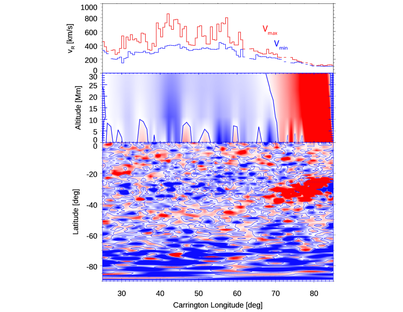
Figure 1: A PFSS model maps the interplanetary magnetic field from the PSP spacecraft during E10 to footpoints within a coronal holes, revealing correlations between the magnetic field in the coronal hole and the radial velocity profile at PSP: in the upper panel the minimum (blue) and maximum (red) radial speed vs longitude; in the second panel the vertical magnetic field at an altitude of 30 Mm above the magnetogram measurements from a PFSS model; and in the bottom panel a map of the magnetic field polarity just above the photosphere, again from the PFSS model. These data indicate that the radial magnetic field is organized into mixed radial polarity intervals on the same scales as the velocity micro-streams observed by PSP (adapted from ).

An alternative to the traditional picture of wave heating of corona as the wind drive mechanism is that magnetic reconnection between open and closed flux, ”interchange reconnection”, directly injects plasma to form the wind (Fisk et al., 1999; Cranmer & van Ballegooijen, 2010). Recent observations of the structure of the fast solar wind close to the sun from NASA’s Parker Solar Probe mission (Fox et al., 2016; Raouafi et al., 2023a) are, for the first time, revealing that the young solar wind is highly structured. The observations yield signatures of the wind drive mechanism that support the role of interchange reconnection in the solar wind drive. First, the radial wind speed is bursty and produces local reversals in the radial magnetic field, ”switchbacks” (Bale et al., 2019). This bursty wind is modulated on spatial scales that are linked to the corresponding spatial structure of the ”supergranulation” network magnetic fields at the base of coronal holes (Bale et al., 2021, 2023) (see Fig. 1). The observations also reveal that peaks in the radial flow speed are correlated with increases in the proton energy with tails up to around 85 keV, an enhanced abundance of alpha particles, and bursty reversals of the radial magnetic field. The modulation of the wind on scales that match that of the network magnetic fields suggests that it is reconnection between closed loops of magnetic flux and open field lines (interchange reconnection) that is the source of energy that drives the wind and the associated modulations (Bale et al., 2021, 2023). This observational data has been used to infer the basic characteristics of interchange reconnection: magnetic fields of around 4.5 $G$, plasma densities of around $10^{9}/cm^{3}$, Alfvén speeds of between 300 and 400 $km/s$, reconnection inflow speeds of around 3$km/s$ (deeply in the collisionless regime), and energy release rates of around $5\times 10^{5}ergs/cm^{2}s$. This rate of energy release is sufficient to power the wind (McKenzie et al., 1995; Axford et al., 1999). A major surprise of these observations was the measurement of a significant energetic ion component with the power-law tails of protons extending above 100$keV$ (Bale et al., 2023). Thus, the solar wind is an ”energetic” wind and the presence of these energetic particles supports the conclusion that the interchange reconnection process driving the wind is collisionless.

Recent solar Extreme UltraViolet (EUV) measurements have revealed ubiquitous jetting activity at the base of the solar corona (Raouafi et al., 2023b). These ”jetlets” are associated with multi-polar regions at the solar surface and have been interpreted as reconnection outflows that are driving the solar wind. These observations further support the idea that reconnection might be playing a role in the drive of the solar wind.

The previous exploration of the acceleration of the solar wind was based on the assumption that the wind velocity started from a very low value (subsonic) in the low corona and increased monotonically to an asymptotic value as $R\rightarrow\infty$. In such a model the radial velocity crosses the sonic point at around $2R_{\odot}$ and the Alfvén point around $8R_{\odot}$. In this traditional picture, the sonic point plays a critical role since it controls whether the wind is able to reach a finite asymptotic velocity or asymptotes to zero velocity at large $R$ (Parker, 1960). However, in a scenario in which interchange reconnection in the low corona drives the wind, the initial injection velocity will be of the order of the Alfvén speed, which in the corona will also be greater than the sound speed. The equations describing how the wind is accelerated from its injection low in the corona to large distances from the sun therefore needs to be re-evaluated in the reconnection drive scenario.

The goal of the present manuscript is therefore to address whether an interchange reconnection solar wind drive scenario is plausible. In exploring such a scenario we include both the Alfvénic injection as well as the expected thermal heating expected from collisionless reconnection in the low corona. We consider specifically the limit in which additional heating of the corona due to Alfvén wave or MHD turbulence is neglected. In Sec. 2 we discuss the basics of a reconnection-based drive mechanism and find a specific estimate for the minimum Alfvén speed required to produce the necessary injection velocity and pressure to power the wind. In Sec. 3 we review the well-known equations describing solar wind acceleration and present the profiles of the radial velocities and other key parameters for a realistic magnetic field profile corresponding to open magnetic flux from a coronal hole. As expected, the velocity profiles depend on a key parameter: the injection velocity compared with the local sound speed, which was the critical parameter in Parker’s original wind model (Parker, 1958, 1960). A significant conclusion is that interchange reconnection will produce a highly structured wind with the radial velocity in some regions rapidly exceeding the local Alfvén speed by a large margin while in other regions the velocity decreases rapidly. In Sec. 4 we develop a set of equations that describe the mixing of adjacent wind streams through the development of the Kelvin-Helmholtz instability. We demonstrate that energy and momentum transfer from a high-energy stream (above the wind threshold) to a low-energy stream (below the wind threshold) can drive the low-energy stream above the wind threshold. The amplitude of the resultant magnetic turbulence is calculated and becomes of the order of the ambient background field. Thus, these strong velocity shear instabilities are the likely source of the Alfvénic turbulence and magnetic ”switchbacks” that are ubiquitous in the young solar wind (Bale et al., 2019; Kasper et al., 2019).

In Sec. 5 we benchmark the profiles of the key plasma parameters with PSP observations at 12.5$R_{\odot}$ and establish that only a small fraction of the plasma ejected upward during interchange reconnection escapes from the sun to form the wind.

2 Basic considerations in an interchange reconnection solar wind drive scenario

The solar escape speed $V_{esc}=\sqrt{2GM_{\odot}/R_{\odot}}\approx 615\text{ km/s}$ greatly exceeds the typical Alfvén speed of 300-400 km/s associated with small-scale interchange reconnection events at the source of the PSP wind observations. Alfvénic outflows from reconnection will therefore not be able to escape solar gravity to form the wind without additional pressure forces. However, the possibility that coronal heating from reconnection combined with Alfvénic injection may be sufficient to drive the wind, even in the absence of additional coronal heating mechanisms, needs to be explored. In the absence of external heating mechanisms, the energy flux of the fluid is a constant (Roberts & Soward, 1972; McKenzie et al., 1995) and yields a Bernoulli-like expression,

$$F_{B}=\frac{1}{2}V^{2}+\frac{5}{2}\frac{P}{\rho}-\frac{GM_{\odot}}{R}=const.,$$ (1)

with $V$ the fluid velocity, $P$ the total pressure, $\rho$ the mass density, and $GM_{\odot}/R$ the solar gravitational potential. For simplicity, we neglect thermal conduction of both electrons and ions. In the absence of additional heat sources, $P/\rho\propto T$ goes to zero at infinity along with the gravitational potential, so a necessary condition for $V$ to remain finite at infinity is for the energy flux to be positive, or

$$\frac{1}{2}V_{0}^{2}+\frac{5}{2}\frac{P_{0}}{\rho_{0}}-\frac{GM_{\odot}}{R_{\odot}}\equiv\frac{1}{2}V_{m}^{2}>0$$ (2)

where the subscripts ”0” denote the values at the base of the corona, which we take to be at the reconnection outflow, and $V_{m}$ is the upper limit on the wind velocity at large distance. During magnetic reconnection, the inflowing energy per particle is given by $B_{0}^{2}/4\pi n_{0}$. Half of the released energy goes into the Alfvénic outflow and around half into ion thermal energy (Eastwood et al., 2013; Haggerty et al., 2018). This yields $V_{0}=V_{A0}$ and $P_{0}=B_{0}^{2}/12\pi$ and the condition in Eq. (2) becomes

$$V_{A0}>\sqrt{3/8}V_{esc}=377km/s.$$ (3)

This is comparable to the estimate of 300-400$km/s$ for the Alfvén speed during interchange reconnection in coronal holes that was obtained from the PSP data (Bale et al., 2023). Specifically, the best estimate for $V_{A}$ came from the comparison of the power-law spectra of protons from SPANi and PIC interchange reconnection simulations, which gave $V_{A}\sim 370~{}km/s$.

3 Solar wind profiles in an interchange reconnection drive scenario

The equations describing the acceleration of the fast wind are well known and become particularly simple in the steady-state limit where heating from Alfvén waves or MHD turbulence is neglected (McKenzie et al., 1995). Because magnetic reconnection in the environment of the corona is expected to be bursty, an extension of the present calculation to include the full time dependence of a bursty driver should be a priority. For simplicity we neglect thermal conduction, which is reasonable for protons because a wind solution requires that the initial flows exceed the sound speed and rapidly become super-Alfvénic. Because the enthalpy flux of ions significantly exceeds that of electrons, as documented in magnetosphere reconnection observations (Eastwood et al., 2013; Phan et al., 2014), the wind drive from electrons is subdominant so treating their dynamics in the simplest possible manner seems justified. A realistic radial profile of the magnetic field emanating from a coronal hole, based on PFSS modeling of the magnetic field connecting the solar surface to PSP during encounter 10 (Bale et al., 2023), is shown in Fig. 2. The source surface of the PFSS model is at 2.5$R_{\odot}$ with a radial dependence of $1/R^{2}$ assumed at larger distances. The expansion rate at low altitude greatly exceeds that based on a simple $1/R^{2}$ model (dashed line in Fig. 2). The super-fast expansion has a significant impact on the rate that pressure drops with radius and therefore the wind acceleration profile.

In a steady state system there are two key invariants, the particle flux, $F_{\rho}$, given by

$$F_{\rho}\equiv\rho V/B,$$ (4)

with $V$ the fluid velocity parallel to the ambient magnetic field, and the energy flux, $F_{w}$, given by

$$F_{w}=F_{\rho}F_{B},$$ (5)

where $F_{B}$ is the Bernoulli-like relation given in Eq. (1). This equation gives an expression for the pressure when the local velocity and radial position are known. The momentum equation along the ambient magnetic field reduces to

$$\frac{\partial}{\partial R}V=-\frac{1}{BF_{\rho}}\frac{\partial}{\partial R}P-\frac{GM_{\odot}}{R^{2}V}.$$ (6)

Eliminating the pressure using Eq. (1), we obtain an equation for the wind velocity $V$,

$$\left(1-\frac{1}{4V^{2}}\left(V_{m}^{2}+\frac{V_{esc}^{2}}{r}\right)\right)\frac{\partial}{\partial r}V^{2}=-\frac{1}{2}\left(V_{m}^{2}-V^{2}+\frac{V_{esc}^{2}}{r}\right)\frac{\partial}{\partial r}\ln B-\frac{3}{4}\frac{V_{esc}^{2}}{r^{2}},$$ (7)

where $r=R/R_{\odot}$ is the normalized radius. The expression within the parentheses on the left hand side (LHS) of the equation goes to zero at the sonic point. To see this we write

$$V^{2}-C_{s}^{2}=V^{2}-\frac{5}{3}\frac{P}{\rho}=\frac{4}{3}V^{2}\left(1-\frac{1}{4V^{2}}\left(V_{m}^{2}+\frac{V_{esc}^{2}}{r}\right)\right),$$ (8)

where we have substituted the pressure from Eq. (1).

For an initial velocity $V_{0}$ below the sound speed, the solution for $V$ always decreases away from the solar surface so there is no wind solution. This can be seen by noting that for $V<C_{S}$ the expression within the parentheses on the LHS of the equation is negative while the RHS of the equation is positive as long as $B$ falls off at least as fast as $1/R^{2}$. Thus, there are no wind solutions that have velocities below the sound speed at the solar surface without an additional source of coronal heating. If, however, $V>C_{S}$ at the solar surface, the velocity will increase with radial distance from the solar surface and reach the terminal wind speed $V_{m}$ at large distances from the sun.

In Fig. 3 we show the numerical solutions of $V(R)$ for a range of initial velocities above and below the sound speed at the solar surface, which was taken to be 350 $km/s$, with the magnetic field profile as shown in Fig. 2. As discussed previously, all of the wind profiles with initial velocities above the sound speed increase sharply and approach limiting velocities at large distances from the solar surface. The peak in the wind velocity, which is relatively close to the solar surface, results from the rapid pressure drop in the expanding magnetic field emanating from the coronal hole. The gradual falloff beyond the peak is a consequence of the sun’s gravitational potential well. In Fig. 4 we show the radial profiles of $V$ (solid), the sound speed $C_{s}$ (dot-dashed) and the Alfvén speed $V_{A}$ (dashed) for the case with $V(R=R_{\odot})=V_{A}(R=R_{\odot})=400~{}km/s$ and $C_{s}(R=R_{\odot})=350~{}km/s$. Both the sound speed and the Alfvén speed decrease rapidly with distance from the surface, which is a consequence of the rapid expansion of $B$ and the corresponding drop in plasma pressure. The consequence is that the expanding wind quickly becomes super-Alfvénic and super-sonic. This will have important consequences for the stability of the wind.

4 A mixing model of solar wind streams

As discussed previously, a wind driven by magnetic reconnection will be highly structured with strong variations in the local outflow velocity. Regions with high outflow and strong heating will have sufficient energy to form an asymptotic wind solution while adjacent regions with low velocity and weak heating will either form a weak outflow or fall back into the chromosphere. Because the Alfvén speed in coronal hole sources falls rapidly with distance above the surface, the flow shear in adjacent regions can exceed the local Alfvén speed and overcome magnetic tension to become Kelvin-Helmholtz (KH) unstable. The resulting mixing is likely to smooth a wind that is highly structured at its source. If sufficient energy is transferred from a high to low energy stream, the low energy stream might gain enough energy to form a wind solution.

To explore how adjacent streams might interact through mixing, we consider a simple model with two adjacent streams that are able to mix their number density, momentum flux, pressure and energy flux. The derivation of the functional form of the mixing term is presented in the Appendix and results in a set of one-dimensional magnetic field aligned equations that are coupled through simple cross-field mixing terms that include the radial separation of the streams as the magnetic field expands away from the solar surface. The three coupled equations for the field aligned velocity $v_{1}$ and $v_{2}$, mass density $\rho_{1}$ and $\rho_{2}$ and pressure $P_{1}$ and $P_{2}$ are for stream 1 as follows: the particle flux, which is no longer constant,

$$\frac{\partial}{\partial R}F_{\rho 1}=M_{\mu}(\Delta\rho)_{2,1},$$ (9)

where for any parameter $H$, $(\Delta H)_{i,j}=H_{i}-H_{j}$; the energy flux, which is also not a constant,

$$\frac{\partial}{\partial R}F_{w1}=M_{\mu}\left[\frac{1}{2}(\Delta\rho v^{2})_{2,1}+\frac{5}{2}(\Delta P)_{2,1}-\frac{GM_{\odot}}{R}(\Delta\rho)_{2,1}\right];$$ (10)

and the momentum flux,

$$\frac{\partial}{\partial R}F_{v1}=-\frac{P_{1}}{B^{2}}\frac{\partial}{\partial R}B-\frac{GM_{\odot}\rho_{1}}{BR^{2}}+M_{\mu}(\Delta\rho v)_{2,1},$$ (11)

where $F_{v1}=F_{\rho 1}v_{1}+P_{1}/B$. Similar equations govern stream 2 with the mixing terms on the right hand side of the equations switched from $(\Delta H)_{2,1}$ to $(\Delta H)_{1,2}$. The mixing term $M_{\mu}$ is given by

$$M_{\mu}=\frac{\mu}{L^{2}B},$$ (12)

with

$$\mu=f_{\mu}\Delta vL\tanh(\Delta v^{2}/V_{A12}^{2}).$$ (13)

$L$ is the spatial separation between the two streams and is parameterized by $L^{2}=L_{0}^{2}B_{0}^{2}/B^{2}$, with $L_{0}$ the separation at the wind source, $\Delta v=|v_{2}-v_{1}|$ and $V_{A12}=(V_{A1}+V_{A2})/2$. The $\tanh$ function in the equation for $\mu$ describes the turn-on of the mixing when the velocity separation $\Delta v$ exceeds the local average Alfvén speed of the two streams. The ad hoc factor $f_{\mu}$ controls the mixing strength, which is typically taken to be $0.1$ (Otto & Fairfield, 2000). The results are relatively insensitive to this value. The mixing velocity that controls the transport between the two streams is taken to be the velocity difference between the two streams above the KH threshold. These equations do not include the energy flux associated with KH turbulence and therefore are only a first step in exploring how solar wind streams might interact. These three equations for $F_{\rho}$, $F_{w}$ and $F_{w}$ can be directly integrated and $\rho$, $v$ and $P$ for each stream can be calculated from these fluxes.

In Fig. 5 we show the velocity profiles of two wind streams, the first being well above the energy threshold to form a wind solution ($v_{1}(R=12.5R_{\odot})\sim 500km/s$) and the second being close to the wind formation threshold ($v_{2}(R=12.5R_{\odot})\sim 100km/s$). The profile of the mean Alfvén speed $V_{A12}$, is shown for comparison. That the velocity difference $\Delta v\gg V_{A12}$ at large $R$ indicates that there is an enormous reservoir of free energy that is likely to produce wind with strong Alfvénic turbulence.

In Fig. 6 we show the velocity profiles of two wind streams in which the mixing between streams is switched on. In this case the first stream is well above the wind threshold while the second stream is below threshold. The corresponding profiles of the energy flux $F_{w1}$ and $F_{w2}$ are shown in Fig. 7. Note that $F_{w2}<0$, confirming that the second stream is below the threshold to form a wind solution. In the absence of mixing, the energy fluxes are independent of radius. The mixing leads to a transfer of energy from the high to the low energy stream so that $F_{w2}>0$ for $R\geq 2R_{\odot}$. The transfer of energy enables the second stream to form a wind solution at large $R$ as shown in Fig. 6. The mean Alfvén speed shown in Fig. 6 confirms that the velocity difference between the two streams approaches the mean Alfvén speed at large $R$. This is confirmed in Fig. 8 where we plot the profile of $(\Delta v/V_{A12})^{2}$. In our simple model we take the mixing velocity $\tilde{v}_{\perp}\simeq(\tilde{B}_{\perp}/B)V_{A12}\simeq\Delta v$ so the curve in Fig. 8 also reveals the profile of $(\tilde{B}_{\perp}/B)^{2}$, where $\tilde{B}_{\perp}$ is the magnetic field fluctuation amplitude. It is because of the rapid decrease in the Alfvén speed due to the expansion of $B$ that the wind becomes strongly turbulent above $2R_{\odot}$.

The development of velocity shear instabilities only occurs if the total shear velocity exceeds the local Alfvén speed. The PSP has recently encountered extended sub-Alfvénic intervals in which the radial velocity falls below the local Alfvén speed (Kasper et al., 2021; Zhao et al., 2022; Bandyopadhyay et al., 2022). These intervals are typically associated with low plasma density and therefore an increase in the local Alfvén speed rather than a significant change in the radial plasma velocity. Analysis suggests that these sub-Alfvénic intervals exhibit fewer switchbacks (Kasper et al., 2021; Bandyopadhyay et al., 2022), as would be expected if velocity shear instabilities were a significant driver of switchbacks.

5 Constraints on the reconnection wind drive mechanism based on PSP observations

The requirements for interchange reconnection driven outflow and heating to drive an outgoing wind are given in Eqs. (2) and (3). The resulting wind solutions shown in Figs. 3 and 4 extend out to 12.5$R_{\odot}$, which overlaps with the distance of closest approach of PSP to the sun. Thus, a comparison of the wind solutions with the local PSP measurements may be able to further constrain the dynamics of the wind drive mechanism.

The E10 data from PSP and associated reconnection modeling suggested that the Alfvén speed $v_{Ar}$ associated with the reconnecting magnetic field during interchange reconnection near the solar surface was around 400$km/s$ (Bale et al., 2023). The profile of the wind velocity in Fig. 4 suggests that the velocity at 12.5$R_{\odot}$ is of the same order, which is consistent with the typical wind velocity measured at this distance from the sun (Bale et al., 2023). However, while the velocity profile in Fig. 4 matches the observational constraints, the Alfvén speed shown in this figure is well below the measured value of around 100$km/s$ (Phan et al., 2022). The magnetic field at 12.5$R_{\odot}$ shown in Fig. 2 of $\approx 600nT$ is consistent with measurements, which implies that the low Alfvén speed is a consequence of the plasma density being too high. Because the entire density profile is controlled by the particle flux in the low corona, the implication is that the density $n_{0}$ at the reconnection site, which was taken to be around $10^{9}/cm^{3}$ in the closed flux region and $10^{8}/cm^{3}$ in the open flux region, is too high. This density was determined from the inferred value of Alfvén speed of interchange reconnection in the low corona of around 370$km/s$ with a magnetic field of 4.5$G$ (Bale et al., 2023).

The Alfvén speed of the reconnecting magnetic field in the low corona is strongly constrained by the PSP observations as is the total magnetic field strength in the low corona. The density could be reduced if the reconnecting component of the magnetic was smaller than the total magnetic field, leaving the Alfén speed based on the reconnecting component of the magnetic field unchanged. However, the powerlaw index of energetic particles produced during reconnection is sensitive to the ratio of the reconnecting to the guide magnetic fields (Arnold et al., 2021; Bale et al., 2023). Indeed, essentially no energetic particles are produced in the strong guide field limit. Thus, reducing the inferred density at the reconnection site by reducing the reconnecting magnetic field component is not an option.

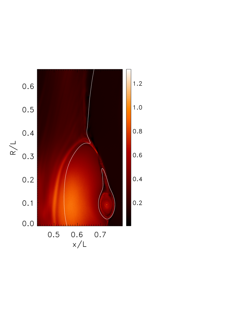
Figure 9: Plasma density from a 2D interchange reconnection simulation. The white line is a newly reconnected magnetic field line. Plasma from the reconnection site (around 0.3$R/L$) is injected onto the open field line at the top of the loop (around 0.37$R/L$) and can flow either back toward the chromosphere or out into the solar wind.

However, while the density at the coronal reconnection site is constrained by the PSP observations, the fraction of that density that escapes from the low corona to form the wind is not. Interchange reconnection actually differs greatly from conventional reconnection in that the reconnection outflow is injected onto a field line with one end anchored in the chromosphere and the other end open. The consequence is that a portion of the reconnection outflow is ejected toward the solar surface while the remainder forms the outward flowing wind. The basic injection geometry is shown in Fig. 9, which is taken from a PIC simulation of interchange reconnection. The details of the reconnection geometry and parameters have been discussed previously (Drake et al., 2021). Shown is the plasma density with the closed flux region on the left (high density) and the open flux region on the right (low density). The dominant reconnection site at the time shown is around $R/L=0.3$. The white line shows a newly reconnected field line that is driving the flux rope toward the solar surface and flow upward. The upward flow splits around $R/L\sim 0.37$ with a portion turning to flow back toward the solar surface and the remainder flowing outward to form the wind. The split in the flow that is evident in Fig. 9 has no counterpart in conventional reconnection. The interchange reconnection geometry at the solar surface is analogous to that at the Earth’s magnetopause where a fraction of the outflow from reconnection is diverted at the cusp toward the ionosphere while the remainder flows away from the Earth into the solar wind.

The simulation of Fig. 9 reveals how a fraction of the exhaust from interchange reconnection near the solar surface is diverted back down to the chromosphere but the simulation does not quantify the fraction that returns to the surface. This would at a minimum require absorbing boundary conditions at the lower boundary of the simulation as well as a complete transport analysis involving both electrons and ions. The ion thermal speed is comparable to the bulk flow as a result of reconnection-driven heating (see the discussion above Eq. (3)) so ion thermal transport must also be included in the analysis.

Thus, while the full analysis of the problem is complex, the lowest order conclusion is not: the distance $L_{inj}$ from the chromosphere to the injection of reconnection exhaust onto the open field at the top of the coronal loops, which is around 10$Mm$ (see Fig. 1), is much smaller than the scale length $L_{P}\sim 700Mm$ of the pressure drop in the outward radial direction (around an $R_{\odot}$ from the falloff of $C_{s}$ in Fig. 4). As a result, only a small fraction of reconnection outflow exhaust will escape to form the wind. If the problem were a simple injection diffusion problem the fraction of escaping plasma would scale like $L_{inj}/L_{P}\sim 0.014$.

That only of the order of $1\%$ of the exhaust outflow escapes to form the wind is actually consistent with the similar problem of the escape of flare driven energetic electrons (SEEs) into the solar wind. Only around $1\%$ or less of non-thermal electrons produced in flares escape into the solar wind (Krucker et al., 2009; Wang et al., 2021).

The expansion ratio from the solar surface to $12.5R_{\odot}$ for the parameters of Fig. 4 is around 650 and is independent of the absolute value of the density. Thus, projecting a plasma density of around $1.5\times 10^{4}/cm^{3}$ from PSP at $12.5R_{\odot}$ yields $n_{0}=1.0\times 10^{7}/cm^{3}$. This is $1\%$ density processed at the reconnection site, which is consistent with the discussion of the previous discussion of the escape fraction. Taking $B_{0}=3.5G$, the resulting total Alfvén speed associated with the escaping fraction is $v_{A0}=2400km/s$.

In Fig. 10 we show the profiles of the plasma density $n$ (solid) and $B$ (dashed) from 1-12.5$R_{\odot}$ starting from $n_{0}=1.0\times 10^{7}/cm^{3}$ and $B_{0}=3.5G$ at the solar surface. Shown in Fig. 11 are the profiles of the velocity $v$, the Alfvén speed $V_{A}$ (based on the total magnetic field) and the sound speed $C_{s}$ for $n$ and $B$ given in Fig. 10 with $v_{0}=400km/s$ and $v_{A0}=2400km/s$. The velocity $v$ exceeds the sound speed $C_{s}$ over the entire profile while the Alfvén point where $v=V_{A}$ is just below $3R_{\odot}$, well below the value of $8R_{\odot}$ typically found in Alfvén wave heating models (McKenzie et al., 1995). On the other hand, there is some observational data from UVCS suggesting that proton outflow velocities from coronal holes reaches 200-300$km/s$ low in the corona (Bemporad, 2017).

6 Discussion and Implications for the development of a highly structured solar wind

Historical models of the solar wind have been based on the premise that the wind starts at very low velocity (subsonic) near the solar surface and is driven solely by the pressure of the coronal plasma. The pressure of the coronal plasma is calculated with a heating model based on the dissipation of Alfvén waves or MHD turbulence. We present an alternate scenario in which magnetic reconnection in the low corona heats the ambient plasma and drives it upwards at the local Alfvén speed. As long as the ejection velocity exceeds the local sound speed (see Fig. 3) and the ejected, heated plasma has sufficiently high pressure (see Eq. (2)), the wind is generated and no additional coronal heating is required. Such ideas have been discussed previously (Fisk et al., 1999; Cranmer & van Ballegooijen, 2010). The approximate minimum condition for interchange reconnection to provide sufficient heating and outflow to overcome gravity to produce the wind is that the Alfvén speed based on the reconnecting magnetic field exceed around 350-400 $km/s$ (see Eq. (3)). This threshold, along with the corresponding expression for the asymptotic wind speed $V_{m}$ given in Eq. (2), clarifies why coronal holes with their relative low density and therefore high relative Alfvén speed are the dominant sources of the fast wind.

The requirement that the interchange reconnection outflow velocity exceed the local sound speed to produce a wind solution has important implications for the basic structure of the wind. The historical view is of a relatively uniform fast wind (McKenzie et al., 1995; Axford et al., 1999) driven by Alfvén wave heating that is broadly distributed over the corona. However, essentially all models of reconnection in macro-scale systems are bursty as a result of the breakup of reconnecting current layers into multiple reconnection sites (Biskamp, 1986; Bhattacharjee et al., 2009; Cassak et al., 2009; Huang & Bhattacharjee, 2010; Karpen et al., 2012). Simulations of interchange reconnection in the low corona also exhibit this bursty behavior (Drake et al., 2021). This translates into a reconnection exhaust that has significant spatial structure (Bale et al., 2023). The consequence is that reconnection outflows at different locations will vary in magnitude – regions with velocities above the sound speed threshold will be accelerated outward and rapidly become super-Alfvénic while adjacent regions with velocities below the sound speed will decelerate (see Fig. 3). The result is a highly structured solar wind that is filamented on scales associated with reconnection burst scales and therefore on smaller scales than the ”super-granulation” network magnetic field. This bursty solar wind has now been extensively documents by PSP observations (Bale et al., 2021, 2023).

Such a fragmented wind will develop at a fraction of a solar radius above the surface (see Fig. 5) but will not survive to large distances. Regions of high Alfvén Mach number flow will be adjacent to regions with very low flow. The interaction of adjacent wind streams has been explored with a simple set of mixing equations (Eqs. (9)-(11)) that are designed to represent the development of the super-Alfvénic Kelvin-Helmholtz instability. A stream with energy above the wind threshold can transfer sufficient energy to a stream with energy below the wind threshold to drive it above threshold (see Figs. 6 and 7). The calculated amplitude of the resulting magnetic field turbulence is a significant fraction of the ambient magnetic field (see Fig. 8). Thus, there is an enormous reservoir of free energy that will drive magnetic turbulence and strong plasma heating that is associated with sheared flows in the structured solar wind. This source is the likely drive mechanism for the associated switchback structure of the magnetic field measured by PSP close to the sun (Kasper et al., 2019; Bale et al., 2019, 2021, 2023).

Thus, it seems likely that, while in the conventional picture magnetic turbulence is injected from near the solar surface and heats the corona to drive the wind, in a reconnection drive scenario it is the free energy of the filamented wind that drives the turbulence. The nature of the resulting turbulence, whether it produces the characteristic switchbacks measured at PSP and its role in further heating the corona to help drive the wind remains to be explored. In support of this idea, the probability of switchback encounters in PSP data-sets is reduced during sub-Alfvénic intervals (Kasper et al., 2021; Bandyopadhyay et al., 2022), which would be expected if velocity shear is a significant driver of switchbacks. Sheared-flow instabilities should be stabilized by magnetic tension in sub-Alfvénic intervals. The basic idea that sheared flows in regions of high Alfvén Mach number could be the source of switchbacks has been proposed (Ruffolo et al., 2020; Schwadron & McComas, 2021) and should continue to be explored.

The mixing model presented here is, of course, highly simplified and only represents the first step in a full exploration of how reconnection drives the solar wind. The present model only treats a time-stationary wind solution. A time-dependent wind drive model needs to be developed with a source that reflects the bursty time-behavior of reconnection. A more complete exploration of the nature and dynamics of the instabilities that develop in the structured wind need to be explored. The present model does not include the energy flux of the magnetic turbulence that is invoked to produce the mixing. Are these shear-flow instabilities capable of producing the characteristic switchbacks seen in observational data?

The typical profiles of the wind velocity $v$, the Alfvén speed $v_{A}$ and sound speed $C_{s}$ are presented in Fig. 11 from the solar surface to $12.5R_{\odot}$. The Alfvén speed matches PSP data only if the plasma density $n_{0}$ near the solar surface is in the range of $10^{7}/cm^{3}$ (see Fig. 10), well below the value of $10^{9}/cm^{3}$ that was inferred from the reconnection characteristics at the solar surface inferred from the PSP E10 observations (Bale et al., 2023). The lower value of $n_{0}$, which is also required to match the measured density at PSP, suggests that only a small fraction of around $1\%$ of the plasma ejected during reconnection ultimately escapes to form the wind. That only such a small fraction of the plasma ejected during reconnection escapes into the solar wind is consistent with similar estimates for the escape of solar energetic electrons (SEEs) from flares into the wind (Krucker et al., 2009; Wang et al., 2021). The profiles shown in Fig. 11 suggest that the wind velocity peaks below $2R_{\odot}$, is relatively flat around 12$R_{\odot}$ and beyond and reaches the Alfvén critical point just above 2$R_{\odot}$. Fast wind observations do suggest flat profiles beyond around 15$R_{\odot}$ (Halekas et al., 2022) but wind profiles close to the solar surface not well established (Kohl et al., 1998; Guhathakurta & Fisher, 1998) but are needed to confirm the high wind acceleration close to the surface. Direct measurements of the outflow speed of Jetlets, which are driven by reconnection close to the solar surface, reveal velocities of around 150$km/s$ in the low corona (Raouafi et al., 2023b). These reconnection-driven structures have been proposed as a solar wind source.

Appendix A Derivation of a mixing model for solar wind streams

Here we show how the phenomenological mixing terms in Eqs. (9)-(11) are calculated. The time-dependent equations describing wind acceleration can be written in the generic form

$$\frac{\partial}{\partial t}F+\boldsymbol{\nabla}\boldsymbol{\cdot}(F{\mathbf{v}})=S,$$ (A1)

where $S$ is a source and $F$ can be the mass density $\rho$, the momentum density $\rho v$, the pressure $P$ or the energy density $\rho v^{2}$ in either of the wind streams. The vector velocity in this equation can be written in terms of perpendicular and parallel components ${\bf v}=v_{\parallel}{\bf b}+\tilde{{\bf v}}_{\perp}$ with ${\bf b}$ the unit vector along the magnetic field and $\tilde{{\bf v}}_{\perp}$ the turbulent velocity field associated with the KH turbulence that drives the transport between adjacent wind streams. We take ${\bf\nabla}\cdot\tilde{{\bf v}}_{\perp}=0$. Equation (A1) can be split between fluctuating and averaged parts using the conventional quasilinear approach. For wind stream $1$ the equation of the average $\langle F_{1}\rangle$ takes the form:

$$\frac{\partial}{\partial t}\langle F_{1}\rangle+{\bf B}\boldsymbol{\cdot}\boldsymbol{\nabla}\left(\frac{\langle F_{1}\rangle v_{1}}{B}\right)+\boldsymbol{\nabla}\boldsymbol{\cdot}\langle\tilde{F}_{1}\tilde{\bf v}_{\perp}\rangle=S_{1}$$ (A2)

with the equation for $\tilde{F}_{1}$ given by

$$\frac{\partial}{\partial t}\tilde{F}_{1}+\tilde{{\bf v}}_{\perp}\boldsymbol{\cdot}{\boldsymbol{\nabla}}\langle F_{1}\rangle=0$$ (A3)

or in integral form:

$$\tilde{F}_{1}=-\left(\int^{t}_{-\infty}d\tau\,\tilde{{\bf v}}_{\perp}(\tau)\right)\boldsymbol{\cdot}\boldsymbol{\nabla}\langle F\rangle,$$ (A4)

where the equations for $\tilde{F}_{1}$ are written in the moving frame of stream $1$. Inserting this result into Eq. (A2), we find

$$\frac{\partial}{\partial t}\langle F_{1}\rangle+{\bf B}\boldsymbol{\cdot}\boldsymbol{\nabla}\left(\frac{\langle F_{1}\rangle v_{1}}{B}\right)-\boldsymbol{\nabla}_{\perp}\boldsymbol{\cdot}\mu\boldsymbol{\nabla}_{\perp}\langle F\rangle=S_{1}$$ (A5)

with

$$\mu=\int^{t}_{-\infty}d\tau\langle\tilde{{\bf v}}_{\perp}(t)\cdot\tilde{{\bf v}}_{\perp}(\tau)\rangle=\langle\tilde{v}_{\perp}^{2}\rangle\tau$$ (A6)

with $\tau$ the correlation time of $\tilde{v}_{\perp}$. We take the transverse scales of both streams to be $L$ and integrate over stream $1$ in the transverse direction to calculate the flux into stream $1$ from stream $2$. The integral over $\langle F_{1}\rangle$ yields $\langle F_{1}\rangle L$ while the integral over the mixing term yields the gradient of $\langle F\rangle$ at the interface $\partial\langle F\rangle/\partial x\simeq(\langle F_{2}\rangle-\langle F_{1}\rangle)/L$. The final equation for $\langle F_{1}\rangle$ takes the form:

$$\frac{\partial}{\partial t}F_{1}+{\bf B}\boldsymbol{\cdot}\boldsymbol{\nabla}\left(\frac{F_{1}v_{1}}{B}\right)-\frac{\mu}{L^{2}}(F_{2}-F_{1})=S_{1},$$ (A7)

where, for simplicity, we have discarded the symbols denoting the average. The mixing term from this generic equation for $F$ yields the forms shown in Eqs. (9)-(11), where in the expression for $\mu$ in Eq. (13) we have taken $\tilde{v}_{\perp}\sim\Delta v$ and $\tau\sim\Delta v/L$ and introduced the onset condition for mixing to occur.

Figure 2: Magnetic field profile (solid line) from the coronal hole of Fig. 1, revealing the fast falloff of the magnetic field compared with the $R^{-2}$ falloff (dashed line).

Figure 3: Radial profile of the solar wind velocity from a solution of Eq. (7) for velocities at $R=R_{\odot}$ of 400$km/s$, 450$km/s$ and 500$km/s$ (solid lines) and for 300$km/s$ (dashed line) for a sound speed at the solar surface of 350$km/s$.

Figure 4: Profiles of the solar wind speed $V$ (solid), sound speed $C_{s}$ (dot-dashed) and Alfvén speed $V_{A}$ (dashed) for an initial velocity of 400$km/s$ and a sound speed of 350$km/s$ at $R=R_{\odot}$.

Figure 5: Radial profile of the solar wind velocity wind streams from a solution of Eq. (7) for velocities at $R=R_{\odot}$ of 500$km/s$ (solid line) and 325$km/s$ (dashed line), corresponding to sound speeds at the solar surface of 350$km/s$ and $300km/s$. The mean Alfvén speed $V_{A12}$ is plotted for comparison (dashed-dot). The mixing term was set to zero in the solutions.

Figure 6: Radial profile of the solar wind velocity wind streams from a solution of Eqs. (9)-(11) for velocities at $R=R_{\odot}$ of 500$km/s$ (solid line) and 275$km/s$ (dashed line), corresponding to sound speeds at the solar surface of 325$km/s$ and $200km/s$. The mean Alfvén speed $V_{A12}$ is plotted for comparison (dashed-dot). The mixing reduced the velocity separation $v_{1}-v_{2}$ to around the mean Alfv́en speed.

Figure 7: Radial profile of the stream energy fluxes $F_{w1}$ and $F_{w2}$ for the simulation profiles shown in Fig. 6. In the absence of mixing, $F_{w}$ is a constant. Because $F_{w2}(R=R_{\odot})$ is negative, stream $2$ would fail to produce an asymptotic wind. The transfer of energy from stream $1$ to stream $2$ as a result of mixing causes $F_{w1}$ to decrease and $F_{w2}$ to increase with radial distance so that $F_{w2}$ becomes positive at large radius and can develop into a wind solution.

Figure 8: Radial profile of $(\Delta v/V_{A12})^{2}=(\tilde{B}_{\perp}/B)^{2})$ corresponding to the simulation of Fig. 7.

Figure 10: Profiles of the plasma density (solid) and magnetic field (dashed) with values of $1.0\times 10^{7}/cm^{3}$ and 3.5$G$ at the solar surface, respectively.

Figure 11: Profiles of the solar wind speed $V$ (solid), sound speed $C_{s}$ (dot-dashed) and Alfvén speed $V_{A}$ (dashed) for a velocity of 400$km/s$ and a sound speed of 350$km/s$ at $R=R_{\odot}$ and other parameters as in Fig. 10.

References

- Arnold et al. (2021) Arnold, H., Drake, J. F., Swisdak, M., et al. 2021, Phys. Rev. Lett., 126, 135101, doi: 10.1103/PhysRevLett.126.135101
- Axford & McKenzie (1992) Axford, W. I., & McKenzie, J. F. 1992, in Solar Wind Seven Colloquium, ed. E. Marsch & R. Schwenn, 1–5
- Axford et al. (1999) Axford, W. I., McKenzie, J. F., Sukhorukova, G. V., et al. 1999, Space Science Rev., 87, 25, doi: 10.1023/A:1005197529250
- Bale et al. (2019) Bale, S. D., Badman, S. T., Bonnell, J. W., et al. 2019, Nature, 576, 237, doi: 10.1038/s41586-019-1818-7
- Bale et al. (2021) Bale, S. D., Horbury, T. S., Velli, M., et al. 2021, arXiv e-prints, arXiv:2109.01069. https://arxiv.org/abs/2109.01069
- Bale et al. (2023) Bale, S. D., Drake, J. F., McManus, M. D., et al. 2023, Nature, 618, 252, doi: 10.1038/s41586-023-05955-3
- Bandyopadhyay et al. (2022) Bandyopadhyay, R., Matthaeus, W. H., McComas, D. J., et al. 2022, ApJ Lett., 926, L1, doi: 10.3847/2041-8213/ac4a5c
- Bemporad (2017) Bemporad, A. 2017, ApJ, 846, 86, doi: 10.3847/1538-4357/aa7de4
- Bhattacharjee et al. (2009) Bhattacharjee, A., Huang, Y.-M., Yang, H., & Rogers, B. 2009, Physics of Plasmas, 16, 112102, doi: 10.1063/1.3264103
- Biskamp (1986) Biskamp, D. 1986, Phys. Fluids, 29, 1520
- Cassak et al. (2009) Cassak, P. A., Shay, M. A., & Drake, J. F. 2009, Physics of Plasmas, 16, 120702, doi: 10.1063/1.3274462
- Cranmer & van Ballegooijen (2010) Cranmer, S. R., & van Ballegooijen, A. A. 2010, ApJ, 720, 824, doi: 10.1088/0004-637X/720/1/824
- De Pontieu et al. (2007) De Pontieu, B., McIntosh, S. W., Carlsson, M., et al. 2007, Science, 318, 1574, doi: 10.1126/science.1151747
- Drake et al. (2021) Drake, J. F., Agapitov, O., Swisdak, M., et al. 2021, A& A, 650, A2, doi: 10.1051/0004-6361/202039432
- Eastwood et al. (2013) Eastwood, J. P., Phan, T. D., Drake, J. F., et al. 2013, Phys. Rev. Lett., 110, 225001, doi: 10.1103/PhysRevLett.110.225001
- Fisk et al. (1999) Fisk, L. A., Schwadron, N. A., & Zurbuchen, T. H. 1999, J. Geophys. Res., 104, 19765, doi: 10.1029/1999JA900256
- Fox et al. (2016) Fox, N. J., Velli, M. C., Bale, S. D., et al. 2016, Space Science Rev., 204, 7, doi: 10.1007/s11214-015-0211-6
- Guhathakurta & Fisher (1998) Guhathakurta, M., & Fisher, R. 1998, ApJ Lett., 499, L215, doi: 10.1086/311371
- Haggerty et al. (2018) Haggerty, C. C., Shay, M. A., Chasapis, A., et al. 2018, Phys. Plasmas, 25, 102120, doi: 10.1063/1.5050530
- Halekas et al. (2022) Halekas, J. S., Whittlesey, P., Larson, D. E., et al. 2022, ApJ, 936, 53, doi: 10.3847/1538-4357/ac85b8
- Huang & Bhattacharjee (2010) Huang, Y.-M., & Bhattacharjee, A. 2010, Physics of Plasmas, 17, 062104, doi: 10.1063/1.3420208
- Karpen et al. (2012) Karpen, J. T., Antiochos, S. K., & DeVore, C. R. 2012, ApJ, 760, 81, doi: 10.1088/0004-637X/760/1/81
- Kasper et al. (2019) Kasper, J. C., Bale, S. D., Belcher, J. W., et al. 2019, Nature, 576, 228, doi: 10.1038/s41586-019-1813-z
- Kasper et al. (2021) Kasper, J. C., Klein, K. G., Lichko, E., et al. 2021, Phys. Rev. Lett., 127, 255101, doi: 10.1103/PhysRevLett.127.255101
- Kohl et al. (1997) Kohl, J. L., Noci, G., Antonucci, E., et al. 1997, Solar Phys., 175, 613, doi: 10.1023/A:1004903206467
- Kohl et al. (1998) —. 1998, ApJ Lett., 501, L127, doi: 10.1086/311434
- Krucker et al. (2009) Krucker, S., Oakley, P. H., & Lin, R. P. 2009, ApJ, 691, 806, doi: 10.1088/0004-637X/691/1/806
- McKenzie et al. (1995) McKenzie, J. F., Banaszkiewicz, M., & Axford, W. I. 1995, A& A, 303, L45
- Neugebauer & Snyder (1962) Neugebauer, M., & Snyder, C. W. 1962, Science, 138, 1095, doi: 10.1126/science.138.3545.1095.a
- Otto & Fairfield (2000) Otto, A., & Fairfield, D. H. 2000, J. Geophys. Res., 105, 21,175, doi: 10.1029/1999JA000312
- Parker (1958) Parker, E. N. 1958, ApJ, 128, 664, doi: 10.1086/146579
- Parker (1960) —. 1960, ApJ, 132, 821, doi: 10.1086/146985
- Parker (1965) Parker, E. N. 1965, Planet Space Sci., 13, 9
- Phan et al. (2014) Phan, T. D., Drake, J. F., Shay, M. A., et al. 2014, Geophys. Res. Lett., 41, 7002, doi: 10.1002/2014GL061547
- Phan et al. (2022) Phan, T. D., Verniero, J. L., Larson, D., et al. 2022, Geophys. Res. Lett., 49, e96986, doi: 10.1029/2021GL096986
- Raouafi et al. (2023a) Raouafi, N. E., Matteini, L., Squire, J., et al. 2023a, Space Sci. Rev., 219, 8, doi: 10.1007/s11214-023-00952-4
- Raouafi et al. (2023b) Raouafi, N. E., Stenborg, G., Seaton, D. B., et al. 2023b, ApJ, 945, 28, doi: 10.3847/1538-4357/acaf6c
- Roberts & Soward (1972) Roberts, P. H., & Soward, A. M. 1972, Proceedings of the Royal Society of London Series A, 328, 185, doi: 10.1098/rspa.1972.0075
- Ruffolo et al. (2020) Ruffolo, D., Matthaeus, W. H., Chhiber, R., et al. 2020, ApJ, 902, 94, doi: 10.3847/1538-4357/abb594
- Schwadron & McComas (2021) Schwadron, N. A., & McComas, D. J. 2021, ApJ, 909, 95, doi: 10.3847/1538-4357/abd4e6
- Wang et al. (2021) Wang, W., Wang, L., Krucker, S., et al. 2021, ApJ, 913, 89, doi: 10.3847/1538-4357/abefce
- Zank et al. (2021) Zank, G. P., Zhao, L. L., Adhikari, L., et al. 2021, Physics of Plasmas, 28, 080501, doi: 10.1063/5.0055692
- Zhao et al. (2022) Zhao, L. L., Zank, G. P., Telloni, D., et al. 2022, ApJ Lett., 928, L15, doi: 10.3847/2041-8213/ac5fb0