Of Mice and Mates: Automated Classification and Modelling of Mouse Behaviour in Groups using a Single Model across Cages

Abstract

Behavioural experiments often happen in specialised arenas, but this may confound the analysis. To address this issue, we provide tools to study mice in the homecage environment, equipping biologists with the possibility to capture the temporal aspect of the individual’s behaviour and model the interaction and interdependence between cage-mates with minimal human intervention. We develop the Activity Labelling Module (ALM) to automatically classify mouse behaviour from video, and a novel Global Behaviour Model (GBM) for summarising their joint behaviour across cages, using a permutation matrix to match the mouse identities in each cage to the model. We also release two datasets, ABODe for training behaviour classifiers and IMADGE for modelling behaviour.

1 Introduction

Understanding behaviour is a key aspect of biology, psychology and social science, e.g. for studying the effects of treatments [1], the impact of social factors [2] or the link with genetics [3]. Biologists often turn to model organisms as stand-ins, of which mice are a popular example, on account of their similarity in genetics, anatomy and physiology [4]. Traditionally, biological studies on mice have taken place in carefully controlled experimental conditions [4], in which individuals are removed from their home-cage, introduced into a specific arena and their response to stimuli (e.g. other mice) investigated: see e.g. [5, 6, 7, 8, 9, 10, 11]. This is attractive because: (a) it presents a controlled stimuli-response scenario that can be readily quantified [12], and (b) it lends itself easier to automated means of behaviour quantification (e.g. through top-mounted cameras in a clutter-free environment [10, 5, 8, 9]).

The downside of such ‘sterile’ environments is that they fail to take into account all the nuances in their behaviour [13]. Such stimuli-response scenarios presume a simple forward process of perception-action which is an over-simplification of their agency [13]. Finally, mice are highly social creatures, and isolating them for specific experiments is stressful and may confound the analysis [14, 15].

In this work, we tackle the problem of studying mice in the home-cage, giving biologists tools to analyse the temporal aspect of an individual’s behaviour and model the interaction between cage-mates — while minimising disruption due to human intervention. Our contributions are: (a) a novel Global Behaviour Model (GBM) for detecting patterns of behaviour in a group setting across cages, (b) the Activity Labelling Module (ALM), an automated pipeline for inferring mouse behaviours in the home-cage from video, and (c) two datasets, ABODe for automated activity classification and IMADGE for analysis of mouse behaviours, both of which we make publicly available. In what follows, we introduce the reader to the relevant literature in Sec. 2, detail our methods in Sec. 3, and describe our datasets in Sec. 4 and document the experiments and results in Sec. 5.

2 Related Work

2.1 Experimental Setups

Animal behaviour has typically been studied over short periods in specially designated arenas (e.g. [5, 7, 6]) and under specific stimulus-response conditions [8]. This simplifies data collection, but may impact behaviour [16] and is not suited to the kind of long-term studies in which we are interested. Instead, newer research uses either an enriched cage [11, 17, 18, 19] or, as in our case, the home-cage itself [14, 20]. Obviously this generates greater challenges for the automation of the analysis, and indeed, none of the systems we surveyed perform automated behaviour classification for individual mice in a group-housed setting.

As relates number of observed individuals, single-mice experiments are often preferred as they are easier to phenotype and control [9, 11, 17, 19]. However, mice are highly social creatures and isolating them affects their behaviour [15], as does handling (often requiring lengthy adjustment periods). Obviously, when modelling social dynamics, the observations must perforce include multiple individuals. Despite this, there are no automated systems that consider the behaviour of each individual as we do. Most research is interested in the behaviour of the group as a whole [7, 21, 22, 23, 24], which circumvents the need to identify the individuals. Carola et al. [25] do model a group setting, but focus on the mother only and how it relates to its litter: similarly, the social interaction test [7, 26] looks at the social dynamics, but only from the point of view of a resident/intruder and in a controlled setting.

2.2 Automated Behaviour Classification

Classifying animal behaviour has lagged behind that of humans, with even recent work using manual labels [6, 25, 27]: even automated methods often require heavy data engineering [28, 7, 24, 11]. Animal behaviour inference tends to be harder because human actions are more recognisable [18], videos are usually less cluttered [29] and most challenges in the human domain focus on classifying short videos rather than long-running recordings as in animal observation [24]. Another factor is the limited number of publicly available animal observation datasets. The few that are accessible are not relevant to our setup: CRIM13 [23] involves only single mice, MARS [26] considers only short snippets, and others like RatSI [30] and MouseAcademy [8] use a top-mounted camera in an open field environment (compared to our side-view recordings in an enriched home cage). We hope, by releasing ABODe, to bridge this gap.

2.3 Modelling Mouse Behaviour

The most common form of behaviour analysis involves reporting summary statistics: e.g. of the activity levels [31], the total duration in each behaviour [20] or the number of bouts [26], effectively throwing away the temporal information. Even where temporal models are used as in [7], this is purely as an aid to the behaviour classification with statistics being still reported in terms of total duration in each state (behaviour). This approach provides an incomplete picture, and one that may miss subtle differences [32] between individuals/groups. Some research output does report ethograms of the activities/behaviours through time [3, 26, 33] (and Bains et al. [14] in particular model this through sinusoidal functions), but none of the works we surveyed consider the temporal co-occurrence of behaviours between individuals in the cage as we do.

An interesting problem that emerges in biological communities is determining whether there is evidence of different behavioural characteristics among individuals/groups [27, 4, 25] or across experimental conditions [32, 14]. Within the statistics and machine learning communities, this is typically the domain of Anomaly detection for which Chandola et al. [34] provide an exhaustive review. This is at the core of most biological studies and takes the form of hypothesis testing for significance [25]. The limiting factor is often the nature of the observations employed, with most studies based on frequency (time spent or counts) of specific behaviours [15, 35]. The analysis in [25] uses a more holistic temporal viewpoint, albeit only on individual mice (our models consider multiple individuals). Wiltschko et al. [9] employ Hidden Markov Models (HMMs) to identify prototypical behaviour (which they compare across environmental and genetic conditions) but only consider pose features — body shape and velocity — and do so only for individual mice. To our knowledge, we are the first to use a global temporal model inferred across cages to flag ‘abnormalities’ in another demographic.

3 Methods

3.1 Data Modalities

Our data stems from a collaboration with the Mary Lyon Centre at MRC Harwell, Oxfordshire (MLC at MRC Harwell), and consists of continuous three-day video and position recordings (using the HCA system [14]) of group-housed mice of the same sex and strain: we focus on male mice of the C57BL/6NTac strain. The home-cage contains bedding, food and water, and is maintained at a regular 12-hour light/dark cycle (lights on at 07:00 and off at 19:00). The mice are housed in groups of three and recorded through an infra-red side-view camera. With no visual markings, the mice are only identifiable through a Radio-Frequency Identification (RFID) tag embedded in them and picked up by a $3\times 6$ antenna-array below the cage. We curated the data to form two datasets (at the 3-month and 1-year age groups), described in Sec. 4.

3.2 Classifying Behaviour: the ALM

Analysing behaviour dynamics in social settings requires knowledge of the individual behaviour throughout the observation period. Our goal is thus to label the activity of each mouse or flag that it is Not Observable at discrete Behaviour Time Intervals (BTIs)— in our case every second. Given the scale of our data, manual labelling is not feasible: instead, our Activity Labelling Module (ALM) (Fig. 1(a)), automatically determines whether each mouse is observable in the video, and if so, infers a probability distribution over which behaviour it is exhibiting. Using discrete time-points simplifies the problem by framing it as a purely classification task, and making it easier to model (Sec. 3.3). We explicitly use a hierarchical label space (observability v. behaviour, Fig. 1(a)f), since (a) it allows us to break down the problem using an Observability Classifier (OC) followed by a Behaviour Classifier (BC) in cascade, and (b) because we prefer to handle Not Observable explicitly as missing data rather than having the BC infer unreliable classifications which can in turn bias the modelling.

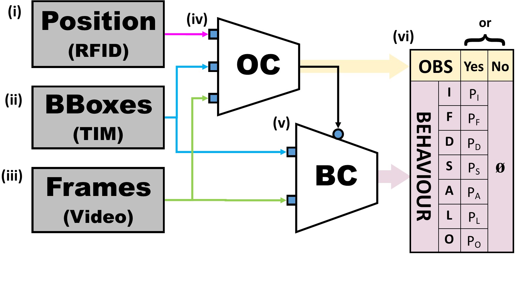
(a) ALM

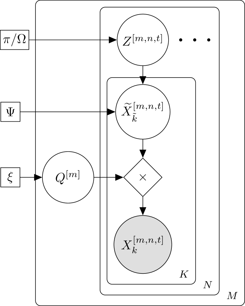
(b) GBM

Figure 1: Model architectures. (a) The ALM for classifying mouse behaviour (vi) from positions (i), BBoxes (ii) and video frames (iii). It is composed of an observability (iv) and behaviour (v) classifier operating in cascade. The TIM is due to [36]. (b) Graphical representation of our GBM. ‘$\times$’ refers to standard matrix multiplication. To reduce clutter, the model is not shown unrolled in time.

Determining Observability.

For the OC we use as features: the position of the mouse (RFID), the fraction of frames (within the BTI) in which a Bounding Box (BBox) for the mouse appears, the average area of such BBoxes and finally, the first 30 Principal Component Analysis (PCA) components from the feature-vector obtained by applying the LFB model [37] to the video. These are fed to a logistic-regression classifier trained using the binary cross-entropy loss [38, 206] with $l_{2}$ regularisation, weighted by inverse class frequency (to address class imbalance). We judiciously choose the operating point (see Sec. 5.1) to balance the errors the system makes.

Probability over Behaviours.

The BC operates only on samples deemed Observable by the OC, outputting a probability distribution over the seven behaviour labels (Sec. 4.1). For each BTI, the centre frame and six others on either side at a stride of eight are combined with the first detection of the mouse in the same period. These are fed to an LFB model [37] (with temperature scaling [39]) finetuned on our data to yield the classification: where there is no detection, a fixed probability distribution is used instead.

3.3 Modelling Behaviour Dynamics

In modelling behaviour, we seek to: (a) capture the temporal aspect of the individual’s behaviour, and (b) model the interaction and interdependence between cage-mates. These goals can be met through fitting a HMM on a per-cage basis, in which the behaviour of each mouse is represented by factorised categorical emissions contingent on a latent ‘regime’ (which couples them together). However, this generates a lot of models, making it hard to analyse and compare observations across cages.

To address this, we seek to fit one Global Behaviour Model (GBM) across cages. The key problem is that the assignment of mouse identities in a cage (denoted as R, G, B) is arbitrary. As an example, if R represents a dominant mouse in one cage, this role may be taken by e.g. mouse G in another cage. Forcing the same emission probabilities across mice avoids this problem, but is too restrictive of the dynamics that can be modelled. Instead, we introduce a permutation matrix to match the mice in any given cage to the GBM as shown in Fig. 1(b).

As in a HMM, there is a latent state $Z$ indexed by cage $m$, recording-run $n$ and time $t$, forming a Markov chain (over $t$), which represents the state of the cage as a whole. This ‘regime’, is parametrised by $\mathbf{\pi}$ in the first time-point (initial probability) as well as $\Omega$ (transition probabilities), and models dependence both in time as well as between individuals. Conditioned on $Z$, $\widetilde{X}$ captures the behaviour of each mouse, through the emission probabilities $\Psi$. Note that $\widetilde{X}$ is indexed over the $K$ mice by $\tilde{k}$ which is a ‘canonical’ assignment.

For each cage $m$, the random variable $Q^{[m]}$ governs which mouse, $k$ (R/G/B) is assigned to which index, $\smash{\tilde{k}}$, in the canonical representation $\smash{\widetilde{X}}$, and is fixed for all samples $n,t$ and behaviours $x$. The sample space of $Q$ consists of all possible permutation matrices of size $K\times K$ i.e. matrices whose entries are 0/1 such that there is only one ‘on’ cell per row/column. $Q$ can therefore take on one of $K!$ distinct values (permutations). This permutation matrix setup has been used previously e.g. in the context of learning inverse graphics representations [40], however here, we are able to use exact inference due to the low dimensionality (in our case $|Q|=3!=6$). Note that fixing $Q$ and $X$ determines $\smash{\widetilde{X}}$ completely by simple linear algebra. This allows us to write out the complete data likelihood as:

$$P_{\Theta}\left(\mathcal{D}\right)=\prod_{m,n}P_{\mathbf{\xi}}\left(Q^{[m]}\right)\left\{P_{\mathbf{\pi}}\left(Z^{[.,1]}\right)\prod_{t=2}^{T^{n}}P_{\Omega}\left(Z^{[.,t]}|Z^{[.,t-1]}\right)\prod_{t=1}^{T^{n}}P_{\Psi}\left(X^{[.,t]}|Z^{[.,t]},Q^{[m]}\right)\right\}.$$ (1)

The parameters $\Theta=\left\{\mathbf{\pi},\Omega,\mathbf{\xi},\Psi\right\}$ of the model are inferred through the Expectation Maximisation (EM) algorithm [41] as shown in Algorithm 1 and detailed in the appendix. Specifically, we use the fact that the posterior over $Q$ is highly peaked to replace the expectation over $Q$ by its maximum, and iterate between fixing $Q$ (per-cage) and optimising the remaining parameters using standard EM.

Algorithm 1 Modified EM for GBM. Equations are in the appendix.

1:$X$$\triangleright$ Observations for all cages

2:$\hat{\mathbf{\xi}},\hat{\Psi},\hat{\mathbf{\pi}},\hat{\Omega}$ $\triangleright$ Initial Parameter Estimates

3:repeat

4:     for all cages $m\in M$ do

5:         $\hat{q}^{[m]}\leftarrow\operatorname*{arg\,max}_{q^{\prime}\in Q^{[m]}}P\left(q^{\prime}|X\right)$ $\triangleright$ Eq. (A.5)

6:         Compute $\widetilde{X}^{[m]}$ given $\hat{q}^{[m]}$ $\triangleright$ Eq. (A.1)

7:     end for

8:     E-Step: Compute Posterior Statistics for $Z$ ($\gamma$, $\eta$) $\triangleright$ Eqs. (A.32 – A.37)

9:     M-Step: Update parameters $\hat{\Psi},\hat{\mathbf{\pi}}$ and $\hat{\Omega}$ $\triangleright$ Eqs. (A.44, A.49, A.54)

10:     Compute Log-Likelihood using new $\hat{\mathbf{\xi}},\hat{\Psi},\hat{\mathbf{\pi}},\hat{\Omega}$ $\triangleright$ Eq. (A.38)

11:until Change in Log-Likelihood $<$ Tolerance

12:Re-Optimise Permutation $\triangleright$ (2: to 5:)

4 Datasets

4.1 ABODe: A dataset for Behaviour Classification

We curated the Annotated Behaviour and Observability Dataset (ABODe) to train and evaluate behaviour classifiers. The dataset, available at https://github.com/michael-camilleri/ABODe consists of 200 two-minute snippets, with 100 for Training, 40 for Validation and 60 for Testing. Each snippet consists of the video, per-mouse locations in the frame and per-second behaviour labels for each of the mice. The per-frame BBox for each mouse is obtained using a TIM [36] which persistently tracks their identity (encoded as R/G/B). The behaviour of each mouse is annotated by a trained phenotyper, and is either Not Observable or one of seven mutually exclusive labels: Immobile, Feeding, Drinking, Self-Grooming, Allo-Grooming, Locomotion or Other. The labelling schema and annotation process are elaborated upon in our Appendix B.3.

4.2 IMADGE: A dataset for Behaviour Analysis

In support of the behaviour analysis of group-housed mice we curated the Individual Mouse Activity Dataset for Group Environments (IMADGE) (available at https://github.com/michael-camilleri/IMADGE). We selected male mice from the C57BL/6NTac strain at the three month (young) and one year (adult) age groups to provide data from two demographics. Since the mice are most active at dawn/dusk, we only use recordings of the 2$\nicefrac{{1}}{{2}}$-hour period around lights-on and lights-off. The clean dataset contains 15 cages (90 recordings) from the adult and ten cages (61 recordings) from the young subset. For each mouse, we provide the mouse position (as picked up by the RFID tag), the average BBox (from TIM [36]), a flag for observability and the probability scores over the behaviour labels (through the ALM, discussed below): all are at a granularity of one-second.

5 Experiments

5.1 Fine-tuning the ALM

The ALM was fit and evaluated on the ABODe dataset.

Metrics.

For both the observability and behaviour components of the ALM we report accuracy and F₁ score [42]. We use the macro-averaged F₁ to better account for the class imbalance. This is particularly severe for the observability classification, in which only about 7% of samples are Not Observable, but it is paramount to flag these correctly. This is because, given that the Observable samples will be used to infer behaviour (Sec. 3.2) which is in turn used to characterise the dynamics of the mice (Sec. 3.3) it is arguably more detrimental to give Unreliable behaviour classifications (i.e. when the sample is Not Observable but the OC deems it to be Observable, which can throw the statistics awry) than missing some Observable periods (which, though Wasteful of data, can generally be smoothed out by the temporal model). This construct is formalised as:

		Predicted
		Obs.	N/Obs.
GT	Obs.	True Observable [TP ]	Wasteful [FN ]
	N/Obs.	Unreliable [FP ]	True Not Observable [TN ]

where GT refers to the ground-truth (annotated) and the standard machine learning terms — True Positive (TP), False Positive (FP), True Negative (TN), False Negative (FN)— are in square brackets. In our evaluation, we report the number of Unreliable and Wasteful samples to take this imbalance into account. For the BC, we also report the normalised (per-sample) log-likelihood score, $\widehat{\mathcal{L}}$, given that we use it as a probabilistic classifier.

Observability.

The challenge in classifying observability was to handle the severe class imbalance, which implied judicious feature selection and classifier tuning. Although the observability sample count is high within ABODe, the skewed nature (with only 7% Not Observable) is prone to overfitting. Features were selected based on their correlation with the observability flag, and narrowed down to the subset already listed (Sec. 3.2). As for classifiers, we explored Logistic Regression (LgR), Naïve Bayes (NB), Random Forests, Support-Vector Machines and feed-forward Neural Networks. Of these, the LgR and NB enveloped all others in the (validation set) ROC curve [42], and were taken forward as candidate methods. These were compared in terms of the number of Unreliable and Wasteful samples at two thresholds: one is at the point at which the number of Wasteful samples is on par with the true number of Not Observable in the data (i.e. 8%), and the other at which the number of predicted Not Observable equals the statistic in the ground-truth data. These appear in Tab. 1(a): the LgR outperforms the NB in almost all cases, and hence we chose the LgR classifier operating at the Wasteful = 8% point.

Table 1: Model Fitting for the ALM. (a) Comparison of LgR and NB (on the validation set) at different operating points. Note that for context, there are 10,124 samples, of which 750 are Not Observable. (b) Evaluation of the Prior (baseline), STLT and LFB models on the Training and Validation sets in terms of Accuracy ($A_{BC}$), macro-F₁ and normalised log-likelihood ($\widehat{\mathcal{L}}$).

	Wasteful = 8%		Equal N/Obs.
	Unrel. $\downarrow$	Waste $\downarrow$	Unrel. $\downarrow$	Waste $\downarrow$
LgR	381	742	499	488
NB	470	750	491	491

(a)

	Train			Validate
	$A_{\text{\lx@glossaries@gls@link{acronym}{bc}{\leavevmode BC}}}\uparrow$	F1 $\uparrow$	$\widehat{\mathcal{L}}\uparrow$	$A_{\text{\lx@glossaries@gls@link{acronym}{bc}{\leavevmode BC}}}\uparrow$	F1 $\uparrow$	$\widehat{\mathcal{L}}\uparrow$
STLT	0.77	0.45	-0.70	0.73	0.36	-1.04
LFB	0.96	0.93	-0.11	0.74	0.61	-2.27

(b)

Behaviour.

We explored two models, the STLT [43] and LFB [37], on the basis of them being most applicable to the spatio-temporal action-localisation problem [44]. In the former case we adapted the architecture to to extend the temporal reach to outwith the BTI, drawing on temporal context from surrounding video frames. We also explored adding in the detections for the cage-mates (with index switching augmentations to encode cage-mate identity symmetry) and the hopper, and feeding in sub-portions of the image relevant to the identified mouse. For the LFB we explored various image augmentation procedures, but not left-right flipping (since we lack symmetry in our fixed setup). For both models, we also investigated lighting enhancement techniques [45], and optimised over batch sizes, learning rates/schedules and frame reach/stride. Given the results on the validation set in Tab. 1(b), with an F₁ of 0.61 (compared to 0.36 for the STLT), the LFB model was chosen as the BC. In samples for which the mouse is not identified by the TIM, but the OC reports that it should be Observable, a categorical distribution was fit instead.

End to End performance.

In Figure 3 we show the performance of the ALM on the held-out test-set: in both cases, we compare against the prior classifier. In terms of observability, the ALM achieves slightly less accuracy but a much higher F₁ score, as it seeks to balance the types of errors (cutting the Unreliable by 34%). In terms of behaviour, when considering only Observable classifications, the system achieves 68% accuracy and 0.54 F₁ despite the high class imbalance. The main culprits for the low score are the grooming behaviours, which as shown in Fig. 3, are often confused for Immobile.

Figure 2: Test performance of the ALM and prior model, in terms of observability and behaviour. Within the former, U and W refer to the counts of Unreliable and Wasteful respectively: for context, there are 20,581 samples.

	Observability				Behaviour
	$A_{\text{\lx@glossaries@gls@link{acronym}{oc}{\leavevmode OC}}}\uparrow$	F1 $\uparrow$	U$\downarrow$	W$\downarrow$	$A_{\text{\lx@glossaries@gls@link{acronym}{bc}{\leavevmode BC}}}\uparrow$	F1 $\uparrow$	$\widehat{\mathcal{L}}\uparrow$
Prior	0.93	0.48	1506	0	0.48	0.09	-1.47
ALM	0.88	0.61	996	1558	0.68	0.54	-1.06

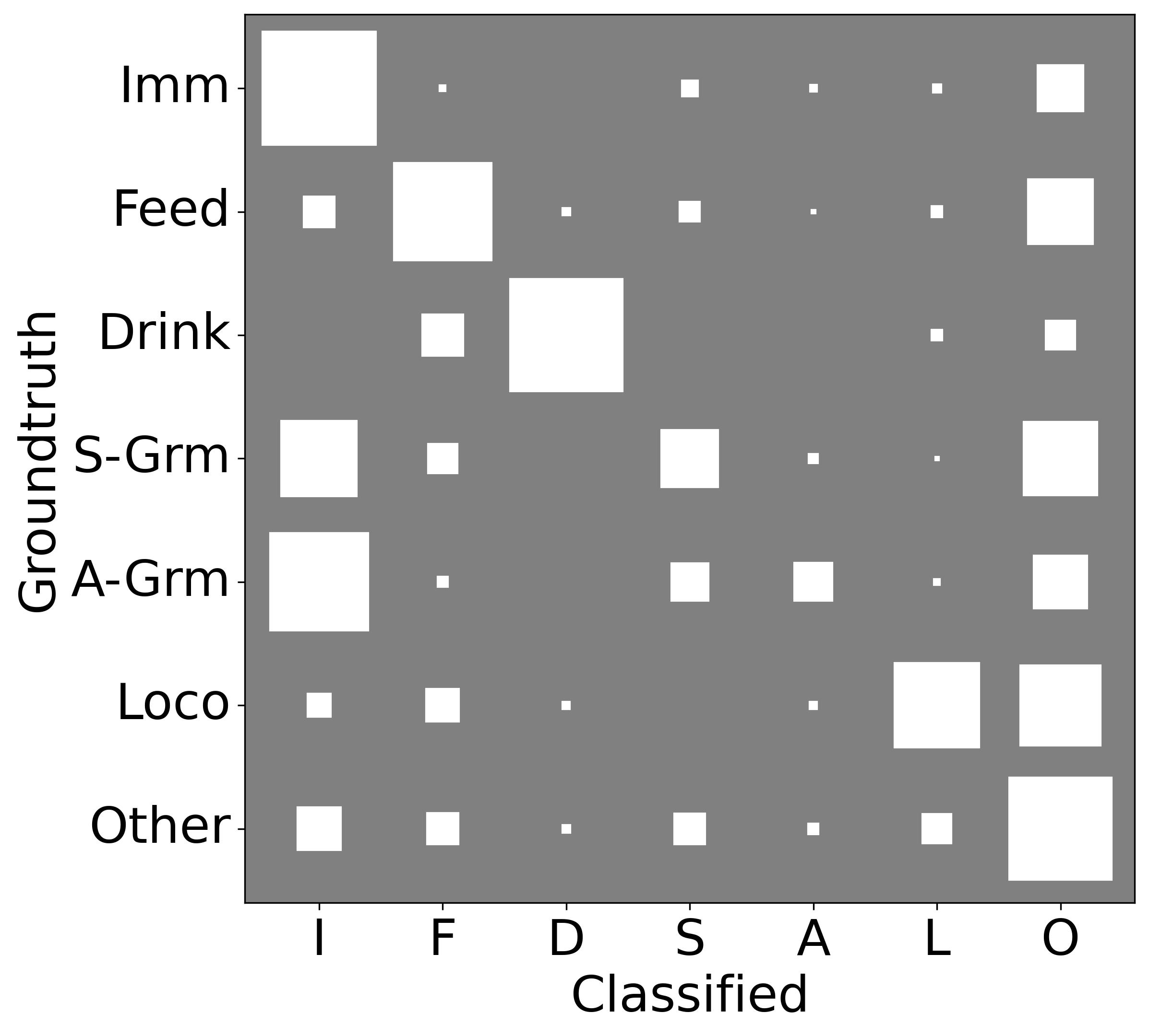
Figure 3: Behaviour confusion matrix.

5.2 Group Behaviour Analysis

The IMADGE dataset is used for our behaviour analysis, focusing on the adult demographic and comparing with the young one later.

Metrics.

We compare models using the normalised log-likelihood $\widehat{\mathcal{L}}$. When reporting relative changes in $\widehat{\mathcal{L}}$, we use a baseline model to set an artificial 0 (otherwise the log-likelihood is not bounded from below). Let $\smash{\widehat{\mathcal{L}}_{BL}}$ represent the normalised log-likelihood of a baseline model — the independent distribution per mouse — and $\smash{\widehat{\mathcal{L}}_{\Theta}}$ respectively for the model of interest (parameterised by $\Theta$). We can then define the Relative Difference in Log-Likelihood (RDL) between two models parameterised by $\Theta$ and $\Theta^{*}$ as:

$$\text{\lx@glossaries@gls@link{acronym}{rdl}{\leavevmode RDL}}\left(\Theta;\Theta^{*}\right)=\left|\frac{\widehat{\mathcal{L}}_{\Theta}-\widehat{\mathcal{L}}_{\Theta^{*}}}{\widehat{\mathcal{L}}_{\Theta}-\widehat{\mathcal{L}}_{BL}}\right|\times 100\%\quad.$$ (2)

Size of $Z$.

The number of latent states $|Z|$ in the GBM governs the expressivity of the model: too small and it is unable to capture all the dynamics, but too large and it becomes harder to interpret. To this end, we fit a per-cage model (i.e. without the $Q$ construct) to the adult mice data for varying $|Z|\in\left\{2,\ldots,13\right\}$, and computed $\widehat{\mathcal{L}}$ on held out data (we used six-fold cross validation). As shown in Fig. 4(a), the likelihood increased gradually, but slowed down beyond $|Z|=7$: we thus use $|Z|=7$ in our analysis.

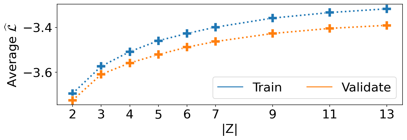
(a)

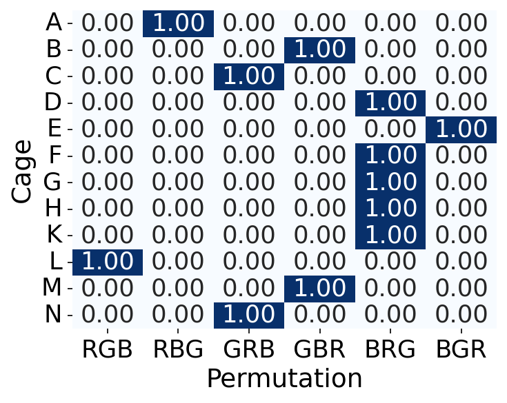
(b)

Figure 4: Tuning of the GBM. (a) Normalised log-likelihood ($\widehat{\mathcal{L}}$) for various dimensionalities of the latent state over all cages. (b) Posterior over $Q$ for all cages ($|Z|=7$, model trained on cage L).

Peaked Posterior over $Q$.

Our Algorithm 1 assumes that the posterior over $Q$ is sufficiently peaked. To verify this, we computed the posterior for all permutations over all cages given each per-cage model. To two decimal places, the posterior is deterministic as shown for model $L$ in Fig. 4(b).

Quality of Fit.

We wished to investigate the penalty paid by using a global rather than per-cage model. To this end, we show in Tab. 2, together with the $\widehat{\mathcal{L}}$ for the data from each cage, the RDL of the GBM compared with that of the per-cage model. The average RDL is 4.8%, which is a reasonable penalty to pay in exchange for a global model. The RDL is less than 5% in all but three cages, A, D and F: cage D in particular exhibited a tendency towards a 6-state regime (data not shown).

Table 2: Normalised log-likelihood ($\widehat{\mathcal{L}}$) of the GBM and RDL on each cage for $|Z|=7$.

	A	B	C	D	E	F	G	H	K	L	M	N
$\widehat{\mathcal{L}}_{\text{\lx@glossaries@gls@link{acronym}{gbm}{\leavevmode GBM}}}$	-1.10	-1.17	-1.16	-1.43	-1.25	-1.36	-1.36	-1.20	-1.13	-1.22	-1.13	-1.29
RDL	5.32	4.56	2.29	11.14	4.94	7.00	4.63	3.17	2.81	2.13	4.61	4.75

Latent Space Analysis.

Figure 5 shows the parameters of the trained GBM. Most regimes have long dwell times. We note that regime F captures the Immobile behaviour for all mice, and is the most prevalent (0.26 steady state probability). The purity of this regime indicates that the mice often are Immobile at the same time, reenforcing the biological knowledge that they tend to huddle together for sleeping, but it is interesting that this was picked up by the model without any apriori bias. Conversely, regime A is most closely associated with the Other label, although it is less pure.

A point of interest are the regimes associated with the Feeding behaviour, that are different across mice — B, E and G for mice 1, 2 and 3 respectively. This is surprising given that more than one mouse can feed at a time (the mouse behaviour researchers at MLC at MRC Harwell indicated that there is no need for competition for feeding resources). This is significant, given that it is a global phenomenon, as it could be indicative of a pecking order in the cage. Another aspect that emerges is the co-occurrence of Self-Grooming with Immobile or Other behaviours: note how in regime (D) (which has the highest probability of Self-Grooming) these are the most prevalent.

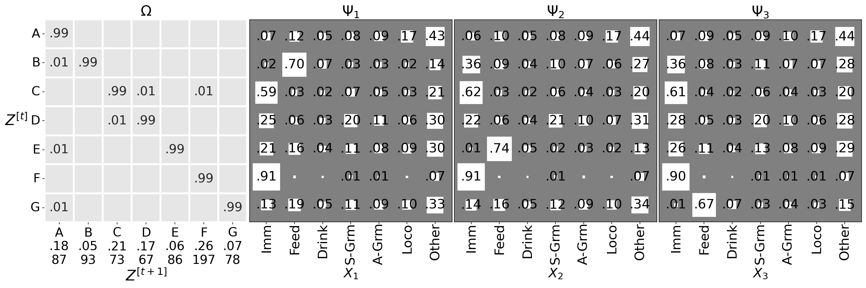
Figure 5: GBM parameters on the Adult mice data for $|Z|=7$. For $\Omega$ (leftmost) we show the transition probabilities: underneath the $Z^{[t+1]}$ labels, we also report the steady-state probabilities (first row) and the expected dwell times (in BTIs, second row). The other three panels show the emission probabilities $\Psi_{k}$ for each mouse as Hinton plots. We omit zeros before the decimal point and suppress values close to 0 (at the chosen precision).

Abnormality Detection.

We used the model trained on our ‘normal’ demographic to analyse data from ‘other’ cages: i.e. abnormality detection. This is useful e.g. to identify unhealthy mice, strain related differences, or, as in our proof of concept, evolution of behaviour through age. In Fig. 6 we show the trained GBM evaluated on data from both the adult (blue) and young (orange) demographics in IMADGE. Apart from two instances, the $\widehat{\mathcal{L}}$ is consistently lower in the younger group compared to the adult demographic: moreover, for cages where we have data in both age groups, $\widehat{\mathcal{L}}$ is always lower for the young mice. Indeed, a binary threshold achieves 90% accuracy when optimised and a T-test on the two subsets indicates significant differences ($p$-value $=1.1\times 10^{-4}$).

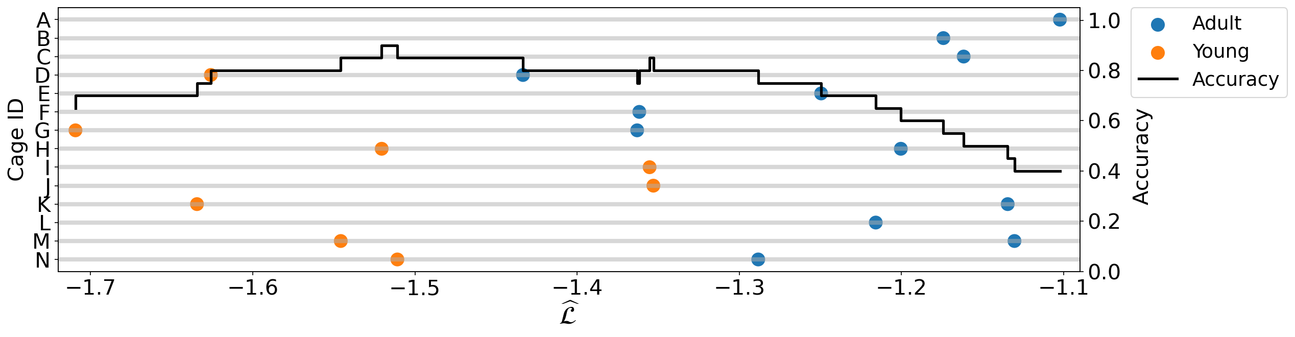
Figure 6: $\widehat{\mathcal{L}}$ scores ($x$-axis) of the GBM on each cage ($y$-axis, left) in the adult/young age groups, together with the accuracy of a binary threshold on the $\widehat{\mathcal{L}}$ (scale on the right).

Analysis of Young mice.

Training the model from scratch on the young demographic brings up interesting different patterns. Firstly, the $|Z|=6$ model emerged as a clear peak this time, as shown in Fig. 7. Figure 8 shows the parameters for the GBM with $|Z|=6$ after optimisation on the young subset. It is noteworthy that the Immobile state is less pronounced (in regime D), which is consistent with the younger mice being more active. Interestingly, while there is a regime associated with Feeding, it is the same for all mice and also much less pronounced: recall that for the adults, the probability of feeding was 0.7 in each of the Feeding regimes. This could indicate that the pecking order, at least at the level of feeding, develops with age.

Figure 7: $\widehat{\mathcal{L}}$ as a function of $|Z|\in\{2,3,...,7\}$, with each cage as initialiser. The average (per $|Z|$) is shown as a blue cross.

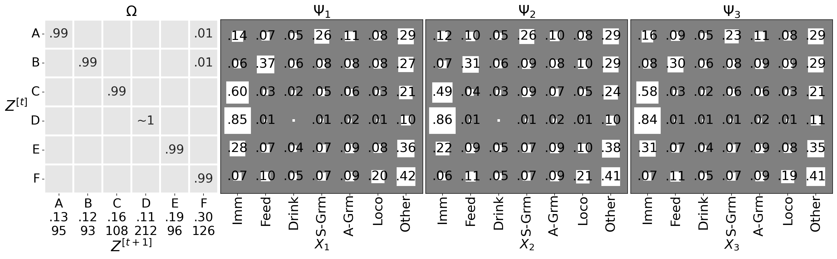
Figure 8: GBM parameters on the Young mice data for $|Z|=6$. Arrangement is as in Fig. 5.

6 Conclusion

In this paper, we have provided a set of tools for biologists to analyse the individual behaviours of group housed mice over extended periods of time. Our main contribution was the novel GBM— a HMM equipped with a permutation matrix for identity matching — to analyse the joint behaviour dynamics across different cages. This evidenced interesting dominance relationships, and also flagged significant deviations in an alternative young age group. In support of the above, we released two datasets, ABODe for training behaviour classifiers and IMADGE for modelling group dynamics (upon which our modelling is based). ABODe was used to develop and evaluate our proposed ALM that automatically classifies seven behaviours despite clutter and occlusion.

Limitations and Future Work:

Since our end-goal was to get a working pipeline to allow us to model the mouse behaviour, the tuning of the ALM leaves room for further exploration, especially as regards architectures for the BC. In future work we would like to analyse other mouse demographics. Much of the pipeline should work “out of the box”, but to handle mice of different colours to those in the current dataset it may be necessary to annotate more data for the ALM (and possibly also for the mouse detector phase of the TIM as provided by Camilleri et al. [36]).

Ethical Approval:

We emphasize that no new data were collected for this study, in line with the Reduction strategy of the 3Rs [46]. The original observations were carried out at MLC at MRC Harwell in accordance with the Animals (Scientific Procedures) Act 1986, UK, Amendment Regulations 2012 (SI 4 2012/3039).

Acknowledgements:

We thank the staff at the MLC at MRC Harwell for providing the raw video and position data, and for their help in interpreting it. We are also grateful to Andrew Zisserman, for his sage advice on architectures for the behaviour classifier of the ALM. MPJC was supported by the EPSRC CDT in Data Science (EP/L016427/1). RSB was supported by funding to MLC from the MRC UK (grant A410).

Appendices

Appendix A Derivations for the Global Behaviour Model

We defined our GBM graphically in Fig. 2 and through Eq. (1) in the main text. Herein we derive the update equations for our modified EM scheme in Algorithm 1.

A.1 Notation

We already defined our key variables in Sect. 3.3 in the main text. However, in order to facilitate our discussion, we make use of the following additional symbols. Firstly, let $\mathbf{Q}^{[m]}$ represent the matrix manifestation (outcome in the sample-space) of the random variable ${Q}^{[m]}$. Secondly, we use $\smash{\mathbb{I}^{[m,n,t]}_{k}}$ to signify that the observation for mouse $k$ from cage $m$ in sample $t$ of run $n$ is not available: i.e. it is missing data. We assume that this follows a Missing-at-Random mechanism [47] which allows us to simply ignore such dimensions: i.e. $\mathbb{I}$ acts as a multiplier such that it zeros out all entries corresponding to missing observations.

A.2 Posterior over $Q$

Due to the deterministic multiplication, selecting a particular $\mathbf{Q}$, and fixing $X$ (because it is observed), completely determines $\smash{\widetilde{X}}$. Formally:

$$\widetilde{X}^{[m,n,t]}=\left.\mathbf{Q}^{[m]}\right.^{\top}\left(X\mathbb{I}\right)^{[m,n,t]},$$ (A.1)

where we have made use of the fact that for a permutation matrix, the inverse is simply the transpose. It follows that:

$$P\left(Q^{[m]}=q|X\right) \propto\sum_{z^{\prime},\tilde{x}^{\prime}}P\left(q,X,z^{\prime},\tilde{x}^{\prime}\right)$$ (A.2)

$$\propto\mathbf{\xi}_{q}\sum_{z^{\prime}}P\left(z^{\prime}\right)\sum_{\tilde{x}^{\prime}}P\left(\tilde{x}^{\prime}|z^{\prime}\right)P\left(X|\tilde{x}^{\prime},q\right)$$ (A.3)

$$\propto\mathbf{\xi}_{q}\sum_{z^{\prime}}P\left(z^{\prime}\right)P\left(\widetilde{X}_{q}|z^{\prime}\right)$$ (A.4)

$$=\frac{\mathbf{\xi}_{q}P\left(\mathbf{Q}^{\top}\left(X\mathbb{I}\right)\right)}{\sum_{q^{\prime}}\mathbf{\xi}_{q}^{\prime}P\left(\mathbf{Q^{\prime}}^{\top}\left(X\mathbb{I}\right)\right)},$$ (A.5)

where in going from Eq. A.3 to Eq. A.4 we made use of the deterministic relationship so that all probabilities over $\tilde{x}$ collapse to 0 if not following the permutation inferred by $q$. In turn, $P\left(\mathbf{Q}^{\top}\left(X\mathbb{I}\right)\right)$ is simply the observed data likelihood of $\smash{\widetilde{X}}$.

A.3 Complete Likelihood and Auxiliary Function

Due to Eq. A.1, we can collapse $X$ and $Q$ into $\widetilde{X}$. Given that we assume the distribution over $Q$ to be sufficiently peaked so that we can pick a single configuration, we can define the complete log-likelihood solely in terms of $Z$ and $\smash{\widetilde{X}}$, much like a HMM but with conditionally independent categorical emissions. Consequently, taking a Bayesian viewpoint and adding priors on each of the parameters, we define the complete data log-likelihood as:

$$P\left(\mathcal{D},\Theta|Q\right)= \prod_{m=1}^{M}\prod_{n=1}^{N}\left(\prod_{z=1}^{|Z|}\mathbf{\pi}_{z}^{Z_{z}^{[m,n,1]}}\prod_{t=2}^{T}\prod_{z^{\prime}=1}^{|Z|}\prod_{z=1}^{|Z|}\Omega_{z^{\prime},z}^{Z_{z^{\prime}}^{[m,n,t-1]}Z_{z}^{[m,n,t]}}\prod_{t=1}^{T}\prod_{z=1}^{|Z|}\prod_{k=1}^{K}\prod_{x=1}^{|\widetilde{X}|}\Psi_{k,z,x}^{\widetilde{X}_{k,x}^{[m,n,t]}}\right)$$

$$\times\text{Dir}\left(\mathbf{\pi};\alpha^{\mathbf{\pi}}\right)\prod_{z=1}^{|Z|}\text{Dir}\left(\Omega_{z};\alpha^{\Omega}_{z}\right)\prod_{k=1}^{K}\prod_{z=1}^{|Z|}\text{Dir}\left(\Psi_{k,z};\alpha^{\Psi}_{k,z}\right),$$ (A.6)

where

$$\text{Dir}\left(\theta;\alpha\right)=\frac{1}{\mathbb{\beta}\left(\alpha\right)}\prod_{i=1}^{|\theta|}\theta_{i}^{\alpha_{i}-1}$$ (A.7)

is the usual Dirichlet prior with the multivariate $\beta$ normaliser function for parameter $\theta\in\left\{\mathbf{\pi},\Omega,\Psi\right\}$. Note that to reduce clutter, we index $\smash{\widetilde{X}}$ using $k$ and $x$ rather than $\tilde{k}/\tilde{x}$.

We seek to maximise the logarithm of the above, but we lack knowledge of the latent regime $Z$. In its absence, we take the Expectation of the log-likelihood with respect to the latest estimate of the parameters ($\hat{\Theta}$) and the observable $\smash{\widetilde{X}}$. We define this expectation as the Auxiliary function, $\mathcal{Q}$:

$$\mathcal{Q}\left(\Theta,\hat{\Theta}\right)\equiv \ \mathbb{E}\left\langle\log\left(P\left(\mathcal{D},\Theta|Q\right)\right)|X,\Theta^{*}\right\rangle$$

$$= \quad\sum_{m=1}^{M}\sum_{n=1}^{N}\left(\sum_{z=1}^{|Z|}\mathbb{E}\left\langle Z_{z}^{[m,n,1]}\right\rangle\log\left(\mathbf{\pi}_{z}\right)+\sum_{t=2}^{T}\sum_{z^{\prime},z}\mathbb{E}\left\langle Z_{z^{\prime}}^{[m,n,t-1]}Z_{z}^{[m,n,t]}\right\rangle\log\left(\Omega_{z^{\prime},z}\right)\right)$$

$$+\sum_{m=1}^{M}\sum_{n=1}^{N}\sum_{t=1}^{T}\sum_{z=1}^{|Z|}\mathbb{E}\left\langle Z^{[m,n,t]}_{z}\right\rangle\sum_{k=1}^{K}\sum_{x=1}^{|\widetilde{X}|}\widetilde{X}_{k,x}^{[m,n,t]}\log\left(\Psi_{k,z,x}\right)$$

$$+\log\left(P\left(\Theta;\mathcal{A}\right)\right)$$ (A.8)

Note that the number of runs $N$ can vary between cages $m\in M$, and similarly, $T$ is in general different for each run $n$: however, we do not explicitly denote this to reduce clutter.

A.4 E-Step

In Eq. A.8 have two expectations, summarised as:

$$\gamma_{z}^{[m,n,t]}=\mathbb{E}\left\langle Z_{z}^{[m,n,t]}\right\rangle =P\left(Z^{[m,n,t]}=z|\widetilde{X}\right)$$ (A.9)

and

$$\eta_{z^{\prime},z}^{[m,n,t]}=\mathbb{E}\left\langle Z_{z^{\prime}}^{[m,n,t-1]}Z_{z}^{[m,n,t]}\right\rangle =P\left(Z^{[m,n,t-1]}=z^{\prime},Z^{[m,n,t]}=z|\widetilde{X}\right).$$ (A.10)

The challenge in computing these is that it involves summing out all the other $z*\notin\left\{z,z^{\prime}\right\}$. This can be done efficiently using the recursive updates of the Baum-Welch algorithm [48], which is standard for HMMs.

A.4.1 Recursive Updates

We first split the dependence around the point of interest $t$. To reduce clutter, we represent indexing over $m/n$ by ‘.’ on the right hand side of equations and summarise the emission probabilities as:

$$P_{\widetilde{X}}^{[m,n]}\left(t,z\right)\equiv\left(\prod_{k=1}^{K}\prod_{x=1}^{|\widetilde{X}|}\Psi_{k,z,x}^{\widetilde{X}_{k,x}^{[.,t]}}\right)$$ (A.11)

Starting with $\gamma$:

$$\gamma_{z}^{[m,n,t]} =\frac{P\left(\widetilde{X}|Z^{[.,t]}_{z}\right)P\left(Z^{[.,t]}_{z}\right)}{P\left(\widetilde{X}\right)}$$ (A.12)

$$=\frac{P\left(\widetilde{X}^{[.,1:t]}|Z^{[.,t]}_{z}\right)P\left(\widetilde{X}^{[.,t+1:T]}|Z^{[.,t]}_{z}\right)P\left(Z^{[.,t]}_{z}\right)}{P\left(\widetilde{X}\right)}$$ (A.13)

$$=\frac{P\left(\widetilde{X}^{[.,1:t]},Z^{[.,t]}_{z}\right)P\left(\widetilde{X}^{[.,t+1:T]}|Z^{[.,t]}_{z}\right)}{P\left(\widetilde{X}\right)}.$$ (A.14)

Similarly, for $$\eta$$:

$$\eta_{z^{\prime},z}^{[m,n,t]} =\frac{P\left(\widetilde{X}|Z^{[.,t-1]}_{z^{\prime}},Z^{[.,t]}_{z}\right)P\left(Z^{[.,t-1]}_{z^{\prime}},Z^{[.,t]}_{z}\right)}{P\left(\widetilde{X}\right)}$$ (A.15)

$$=\frac{P\left(\widetilde{X}^{[.,1:t-1]}|Z^{[.,t-1]}_{z^{\prime}}\right)P_{\widetilde{X}}^{[.]}\left(t,z\right)P\left(\widetilde{X}^{[.,t+1:T]}|Z^{[.,t]}_{z}\right)P\left(Z^{[.,t-1]}_{z^{\prime}}\right)\Omega_{z^{\prime},z}}{P\left(\widetilde{X}\right)}$$ (A.16)

$$=\frac{P\left(\widetilde{X}^{[.,1:t-1]},Z^{[.,t-1]}_{z^{\prime}}\right)P_{\widetilde{X}}^{[.]}\left(t,z\right)P\left(\widetilde{X}^{[.,t+1:T]}|Z^{[.,t]}_{z}\right)\Omega_{z^{\prime},z}}{P\left(\widetilde{X}\right)}$$ (A.17)

We see that now we have two ‘messages’ that crucially can be defined recursively. Let the ‘forward’ pass be denoted by $F$ as:

$$F^{[m,n,t]}_{z} =P\left(\widetilde{X}^{[.,1:t]},Z^{[.,t]}_{z}\right)$$ (A.18)

$$=\sum_{z^{\prime}=1}^{|Z|}P\left(\widetilde{X}^{[.,1:t-1]},Z^{[.,t-1]}_{z^{\prime}}\right)P\left(Z^{[.,t]}_{z}|Z^{[.,t-1]}_{z^{\prime}}\right)P\left(\widetilde{X}^{[.,t]}|Z^{[.,t]}_{z}\right)$$ (A.19)

$$=P_{\widetilde{X}}^{[.]}\left(t,z\right)\sum_{z^{\prime}=1}^{|Z|}F^{[.,t-1]}_{z^{\prime}}\Omega_{z^{\prime},z}.$$ (A.20)

For the special case of $$t=1$$, we have:

$$F^{[m,n,1]}_{z} =\mathbf{\pi}_{z}P_{\widetilde{X}}^{[.]}\left(1,z\right).$$ (A.21)

Similarly, we denote the ‘backward’ recursion by $B$:

$$B^{[m,n,t]}_{z} =P\left(\widetilde{X}^{[.,t+1:T]}|Z^{[.,t]}_{z}\right)$$ (A.22)

$$=\sum_{z^{\prime}=1}^{|Z|}P\left(Z^{[.,t+1]}_{z^{\prime}}|Z^{[.,t]}_{z}\right)P\left(\widetilde{X}^{[.,t+1]}|Z^{[.,t+1]}_{z^{\prime}}\right)P\left(\widetilde{X}^{[.,t+2:T]}|Z^{[.,t+1]}_{z^{\prime}}\right)$$ (A.23)

$$=\sum_{z^{\prime}=1}^{|Z|}\Omega_{z,z^{\prime}}P_{\widetilde{X}}^{[.]}\left(t+1,z\right)B^{[.,t+1]}_{z^{\prime}}.$$ (A.24)

Again, we have to consider the special case for $t=T$:

$$B^{[m,n,T]}_{z}=1.$$ (A.25)

Scaling Factors

To avoid numerical underflow, we work with normalised distributions. Specifically, we define:

$$\hat{F}^{[m,n,t]}_{z}=P\left(Z^{[.,t]}_{z}|\widetilde{X}^{[.,1:t]}\right)=\frac{F^{[.,t]}_{z}}{P\left(\widetilde{X}^{[.,1:t]}\right)}.$$ (A.26)

We relate these factors together through:

$$S^{[m,n,t]}=P\left(\widetilde{X}^{[.,t]}|\widetilde{X}^{[.,1:t-1]}\right),$$ (A.27)

and hence, from the product rule, we also have:

$$P\left(\widetilde{X}^{[m,n,1:t]}\right)=\prod_{\tau=1}^{t}S^{[.,\tau]}.$$ (A.28)

Consequently, we can redefine:

$$\hat{F}^{[m,n,t]}_{z} =\frac{F^{[.,t]}_{z}}{\prod_{\tau=1}^{t}S^{[.,\tau]}}$$ (A.29)

and

$$\hat{B}^{[m,n,t]}_{z} =\frac{B^{[.,t]}_{z}}{\prod_{\tau=t+1}^{T}S^{[.,\tau]}}$$ (A.30)

We denote for simplicity

$$C^{[m,n,t]}=\left(S^{[.,t]}\right)^{-1}$$ (A.31)

as the normaliser for the probability. This allows us to redefine the recursive updates for the responsibilities as follows:

$$\gamma_{z}^{[m,n,t]} =\hat{F}^{[.,t]}_{z}\hat{B}^{[.,t]}_{z},$$ (A.32)

and

$$\eta_{z^{\prime},z}^{[m,n,t]} =C^{[.,t]}\hat{F}^{[.,t-1]}_{z^{\prime}}\hat{B}_{z}^{[.,t]}\Omega_{z^{\prime},z}P_{\widetilde{X}}^{[.]}\left(t,z\right),$$ (A.33)

where:

$$\hat{F}^{[m,n,t]}_{z} =C^{[.,t]}\ddot{F}^{[.,t]}_{z}$$ (A.34)

$$\ddot{F}^{[m.n,t]}_{z} =\begin{cases}P_{\widetilde{X}}^{[.]}\left(1,z\right)\mathbf{\pi}_{z}&\text{if}\quad t=1,\\ P_{\widetilde{X}}^{[.]}\left(t,z\right)\sum_{z^{\prime}=1}^{|Z|}\hat{F}^{[.,t-1]}_{z^{\prime}}\Omega_{z^{\prime},z}&\text{otherwise}\end{cases}$$ (A.35)

$$C^{[m,n,t]} =\left(\sum_{z^{\prime}=1}^{|Z|}\ddot{F}^{[.,t]}_{z^{\prime}}\right)^{-1}$$ (A.36)

$$\hat{B}^{[m,n,t]}_{z} =\begin{cases}1&\text{if}\quad t=T,\\ C^{[.,t+1]}\sum_{z^{\prime}=1}^{|Z|}\Omega_{z,z^{\prime}}P_{\widetilde{X}}^{[.]}\left(t+1,z\right)\hat{B}^{[.,t+1]}_{z^{\prime}}&\text{otherwise}\end{cases}.$$ (A.37)

Through the normalisers $C$, we also compute the observed data log-likelihood:

$$\log\left(P\left(\widetilde{X};\Theta\right)\right)=-\sum_{m=1}^{M}\sum_{n=1}^{N}\sum_{t=1}^{T}\log\left[C^{[.,t]}\right].$$ (A.38)

A.5 M-Step

We re-arrange the $\mathcal{Q}$-function to expand and split all terms according to the parameter involved (to reduce clutter we collapse the sum over $M/N$ and ignore constant terms):

$$\mathcal{Q}\left(\Theta,\hat{\Theta}\right)= \quad\sum_{m,n}\sum_{z=1}^{|Z|}\gamma_{z}^{[.,1]}\log\left(\mathbf{\pi}_{z}\right)+\sum_{z=1}^{|Z|}\left(\alpha^{\mathbf{\pi}}_{z}-1\right)\log\left(\mathbf{\pi}_{z}\right)$$

$$+\sum_{m,n}\sum_{t=2}^{T}\sum_{z^{\prime},z}\eta_{z^{\prime},z}^{[.,t]}\log\left(\Omega_{z^{\prime},z}\right)+\sum_{z^{\prime},z}\left(\alpha^{\Omega}_{z^{\prime},z}-1\right)\log\left(\Omega_{z^{\prime},z}\right)$$

$$+\sum_{m,n}\sum_{t=1}^{T}\sum_{z=1}^{|Z|}\gamma^{[.,t]}_{z}\sum_{k=1}^{K}\sum_{x=1}^{|\widetilde{X}|}{\widetilde{X}^{[.,t]}_{k,x}}\log\left(\Psi_{k,z,x}\right)+\sum_{z=1}^{|Z|}\sum_{k=1}^{K}\sum_{x=1}^{|\widetilde{X}|}\left(\alpha^{\Psi}_{k,z,x}-1\right)\log\left(\Psi_{k,z,x}\right)$$

$$+Const$$ (A.39)

A.5.1 Maximising for $\mathbf{\pi}$

Since we have a constraint ($\mathbf{\pi}$ must be a valid probability that sums to 1) we maximise the constrained Lagrangian:

$$\Lambda=\mathcal{Q}+\lambda\left(\sum_{z^{\prime}=1}^{|Z|}\mathbf{\pi}_{z^{\prime}}-1\right).$$ (A.40)

We maximise this by taking the derivative with respect to $\mathbf{\pi}_{z}$ and setting it to 0 (note that we can zero-out all terms involving $z^{\prime}\neq z$ which are constant with respect to $\mathbf{\pi}_{z}$):

$$\frac{\partial\Lambda}{\partial\mathbf{\pi}_{z}} =\frac{1}{\mathbf{\pi}_{z}}\left(\sum_{m=1}^{M}\sum_{n=1}^{N}\gamma^{[m,n,1]}_{z}+\alpha^{\mathbf{\pi}}_{z}-1\right)+\lambda=0$$ (A.41)

$$\lambda\mathbf{\pi}_{z} =-\sum_{m=1}^{M}\sum_{n=1}^{N}\gamma^{[m,n,1]}_{z}-\alpha^{\mathbf{\pi}}_{z}+1$$ (A.42)

Summing the above over $$z$$:

$$\lambda =-\sum_{m=1}^{M}\sum_{n=1}^{N}\sum_{z^{\prime}=1}^{|Z|}\gamma^{[m,n,1]}_{z^{\prime}}-\sum_{z^{\prime}=1}^{|Z|}\alpha^{\mathbf{\pi}}_{z^{\prime}}+|Z|$$

$$=-\sum_{m=1}^{M}N^{m}-\sum_{z^{\prime}=1}^{|Z|}\alpha^{\mathbf{\pi}}_{z^{\prime}}+|Z|$$ (A.43)

In the above we have made use of the fact that both $\mathbf{\pi}_{z}$ and $\gamma_{z}^{[n]}$ sum to 1 over $z^{\prime}$. Substituting Eq. (A.43) for $\lambda$ in Eq. (A.42) we get the maximum-a-posteriori estimate for $\hat{\mathbf{\pi}}_{z}$:

$$\hat{}\mathbf{\pi}_{z}=\frac{\sum_{m=1}^{M}\sum_{n=1}^{N}\gamma^{[m,n,1]}_{z}+\alpha^{\mathbf{\pi}}_{z}-1}{\sum_{m=1}^{M}N^{m}+\sum_{z^{\prime}=1}^{|Z|}\alpha^{\mathbf{\pi}}_{z^{\prime}}-|Z|}.$$ (A.44)

A.5.2 Maximising for $\Psi$

We follow a similar constrained optimisation procedure for $\Psi$, with the Lagrangian:

$$\Lambda=\mathcal{Q}+\sum_{k^{\prime},z^{\prime}}\lambda_{k^{\prime},z^{\prime}}\left(\sum_{x^{\prime}}\Psi_{k^{\prime},z^{\prime},x^{\prime}}-1\right)$$ (A.45)

Taking the derivative of Eq. (A.45) with respect to $\Psi_{k,z,x}$ and setting it to 0 (ignoring constant terms):

$$\frac{\partial\Lambda}{\partial\Psi_{k,z,x}} =\frac{1}{\Psi_{k,z,x}}\left(\sum_{m=1}^{M}\sum_{n=1}^{N}\sum_{t=1}^{T}\gamma^{[m,n,t]}_{z}\widetilde{X}^{[m,n,t]}_{k,x}+\alpha^{\Psi}_{k,z,x}-1\right)+\lambda_{k,z}=0$$ (A.46)

$$\lambda_{k,z}\Psi_{k,z,x} =-\sum_{m=1}^{M}\sum_{n=1}^{N}\sum_{t=1}^{T}\gamma^{[m,n,t]}_{z}\widetilde{X}^{[m,n,t]}_{k,x}-\alpha^{\Psi}_{k,z,x}+1$$ (A.47)

Again, summing this over $$x^{\prime}$$ yields:

$$\lambda_{k,z} =-\sum_{m=1}^{M}\sum_{n=1}^{N}\sum_{t=1}^{T}\gamma^{[m,n,t]}_{z}\sum_{x^{\prime}=1}^{|\widetilde{X}|}\widetilde{X}^{[m,n,t]}_{k,x^{\prime}}-\sum_{x^{\prime}=1}^{|\widetilde{X}|}\alpha^{\Psi}_{k,z,x^{\prime}}+|\widetilde{X}|$$ (A.48)

Substituting Eq. (A.48) back into Eq. (A.47) gives us:

$$\hat{\Psi}_{k,z,x}=\frac{\sum_{m=1}\sum_{n=1}^{N}\sum_{t=1}^{T}\gamma^{[m,n,t]}_{z}\widetilde{X}^{[m,n,t]}_{k,x}+\alpha^{\Psi}_{k,z,x}-1}{\sum_{m=1}^{M}\sum_{n=1}^{N}\sum_{t=1}^{T}\gamma^{[m,n,t]}_{z}\sum_{x^{\prime}=1}^{|\widetilde{X}|}\widetilde{X}^{[m,n,t]}_{k,x^{\prime}}+\sum_{x^{\prime}=1}^{|\widetilde{X}|}\alpha^{\Psi}_{k,z,x^{\prime}}-|\widetilde{X}|}.$$ (A.49)

A.5.3 Maximising for $\Omega$

As always, this is a constrained optimisation by virtue of the need for valid probabilities. We start from the Lagrangian:

$$\Lambda =\mathcal{Q}+\sum_{z^{\dagger}=1}^{|Z|}\lambda_{z^{\dagger}}\left(\sum_{z^{*}=1}^{|Z|}\Omega_{z^{\dagger},z^{*}}-1\right)$$ (A.50)

$$\frac{\partial\Lambda}{\partial\Omega_{z^{\prime},z}} =\frac{1}{\Omega_{z^{\prime},z}}\left(\sum_{m=1}^{M}\sum_{n=1}^{N}\sum_{t=2}^{T}\eta_{z^{\prime},z}^{[.,t]}+\left(\alpha^{\Omega}_{z^{\prime},z}-1\right)\right)+\lambda_{z^{\prime}}$$ (A.51)

$$\lambda_{z^{\prime}}\Omega_{z^{\prime},z} =-\left(\sum_{m=1}^{M}\sum_{n=1}^{N}\sum_{t=2}^{T}\eta_{z^{\prime},z}^{[.,t]}+\left(\alpha^{\Omega}_{z^{\prime},z}-1\right)\right)$$ (A.52)

$$\lambda_{z^{\prime}} =-\left(\sum_{m=1}^{M}\sum_{n=1}^{N}\sum_{t=2}^{T}\sum_{z^{*}=1}^{|Z|}\eta_{z^{\prime},z^{*}}^{[.,t]}+\sum_{z^{*}=1}^{|Z|}\alpha^{\Omega}_{z^{\prime},z^{*}}-|Z|\right)$$ (A.53)

which after incorporating into the previous equation gives the maximum-a-posteriori update:

$$\hat{\Omega}_{z^{\prime},z}=\frac{\sum_{m=1}^{M}\sum_{n=1}^{N}\sum_{t=2}^{T}\eta_{z^{\prime},z}^{[.,t]}+\left(\alpha^{\Omega}_{z^{\prime},z}-1\right)}{\sum_{m=1}^{M}\sum_{n=1}^{N}\sum_{t=2}^{T}\sum_{z^{*}=1}^{|Z|}\eta_{z^{\prime},z^{*}}^{[.,t]}+\sum_{z^{*}=1}^{|Z|}\alpha^{\Omega}_{z^{\prime},z^{*}}-|Z|}$$ (A.54)

Appendix B Elaboration on the Datasets

We describe our derived datasets in more detail.

B.1 A Note on the original Data

In line with the Reduction strategy of the 3Rs [46] we reuse existing data available through MLC at MRC Harwell. To this end, an understanding of the raw data helps in our discussion to follow.

B.1.1 Husbandry

The data pertains to male and female mice from several strains (although we focus on male mice from the C57BL/6NTac strain). Mice of the same sex and strain are housed in groups of three as a unique cage throughout their lifetime. To reduce the possibility of impacting social behaviour [13], the mice have no distinguishing external visual markings: instead, they were microchipped with unique RFID tags placed in the lower part of their abdomen. All recordings happen in the group’s own home-cage, thus minimising disruption to their life-cycle. Apart from the mice, the cage contains a food and drink hopper, bedding and a movable tunnel. For each cage (group of three mice), three to four day continuous recordings are performed when the mice are 3-months, 7-months, 1-year and 18-months old. During monitoring, the mice are kept on a standard 12-hour light/dark cycle with lights-on at 07:00 and lights-off at 19:00.

B.1.2 Data Modalities

The recordings come in two modalities: video and position. The recordings are split into 30-minute segments to be more manageable, with RFID and video synchronised accordingly. Experiments are thus identified uniquely by the cage-id to which they pertain, the age group at which they are recorded and the segment number.

Video

An infra-red camera captures video at 25 frames per second from a side-mounted viewpoint and stores it as compressed $1280\times 720$ greyscale (single-channel) MP4 files. Understandably, the hopper itself is opaque and this impacts the lighting (and ability to resolve objects) in the lower right quadrant. As regards cage elements, the hopper itself is static, and the mice can feed either from the left or right entry-points. The water-spout is on the left of the hopper towards the back of the cage from the provided viewpoint. The bedding itself consists of shavings and is highly dynamic, with the mice occasionally burrowing underneath it. Similarly, the cardboard tunnel roll can be moved around or chewed and varies in appearance throughout recordings.

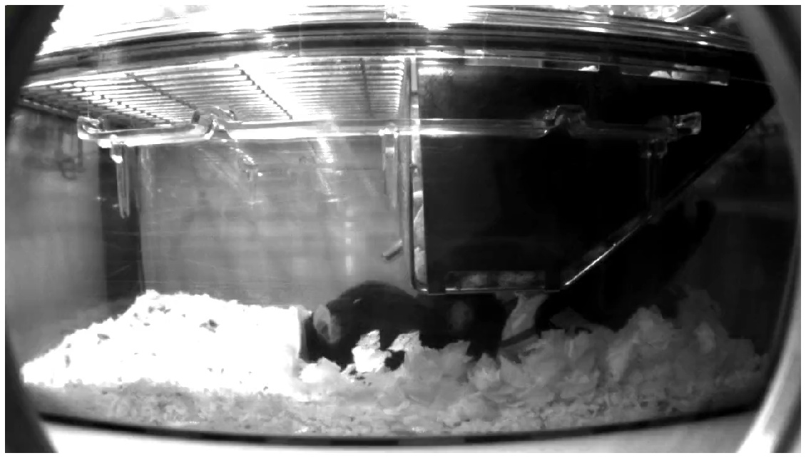
(a) Raw Video

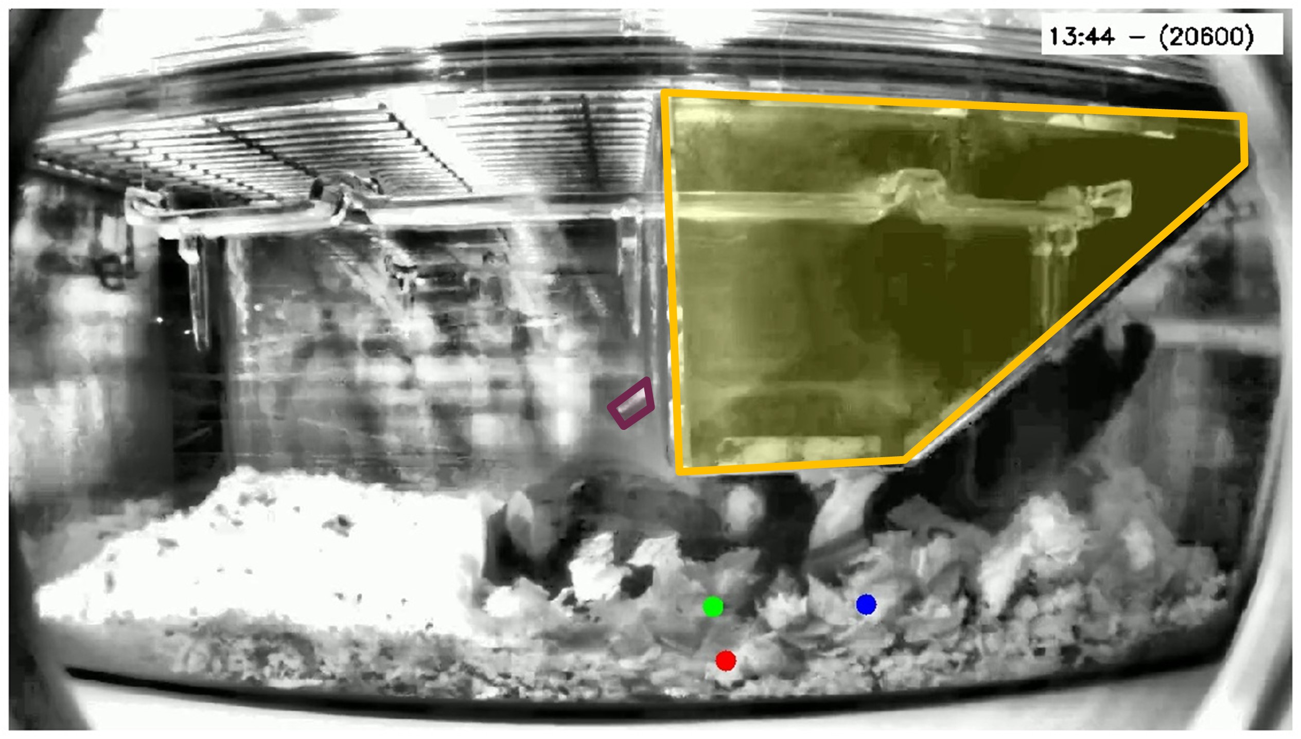
(b) Enhanced video

Figure B.1: Example Video frames from our data, showing (a) the raw frame and (b) and enhanced visual using CLAHE [49]. In (b) the hopper is marked in yellow and the water spout in purple, while the (RFID) mouse positions are projected into image space and overlaid as red, green and blue dots.

Position:

The mice are uniquely identified through an RFID implant. Mice within the same cage are sorted in ascending order by their identifier and denoted Red/Green and Blue for visualisation and reference purposes. The baseplate contains 18 receivers, arranged in a $3\times 6$ grid. The antennas are successively scanned in numerical order to test for the presence of a mouse: the baseplate does on average 2.5 full-scans per-second.

B.2 Individual Mouse Activity Dataset for Group Environments (IMADGE)

We aimed to provide general tools for analysing mouse behaviour in group settings. The IMADGE is our curated selection of data, including automatically-generated localisation and behaviour labels for the mice in the cage to allow us to answer the proposed research questions. The dataset also forms the basis for the ABODe dataset (Sec. B.3).

B.2.1 Data Selection

Demographics:

We use data exclusively from the male C57BL/6NTac at the 3-month and 1-year age groups. This choice was motivated by the goal of having as much data as possible. The most prevalent single group in the MLC at MRC Harwell dataset was the male C57BL/6NTac recorded at 1-year of age. Contingent on the above choice, a related demographic was sought to provide some variability (e.g. for testing our anomaly detection schemes). On the advice of the biologists at MLC at MRC Harwell, and in an effort to minimise statistical shift for the algorithms to work on (e.g. same fur colour), we picked the same male C57BL/6NTac strain, but at the 3-month old time point. After discarding some recordings with non-standard setups, we ended up with 15 cages from the Adult (1-year) and 10 from the Young (3-month) age groups. Particularly, nine of the cages exist in both subsets and thus are useful for comparing behaviour dynamics longitudinally.

Choice of Segments

The mice under study (C57BL/6NTac) are crepuscular, meaning that they are most active during dawn/dusk: i.e. the periods at which light turns to dark or vice versa. This is particularly relevant, because changes in the onset/offset of activity around these times can be very good early predictors of e.g. neurodegenerative conditions [50]. Consequently, we selected segments that overlap to any extent with the morning (06:00-08:00) and evening (18:00-20:00) periods, resulting in generally 2$\nicefrac{{1}}{{2}}$ hour recording runs. This gave us 6 runs per-cage.

B.2.2 Derived Data

Apart from the existing video and (RFID) position data, IMADGE exposes additional information: the localisation of each mouse in the video, an indication of whether it is observable or not, and a classification score for its behaviour.

Common Frame of Reference:

Using pre-recorded calibration videos available with the raw data, we annotated fixed points on the base-plate and optimised a similarity transform to map videos from different cages into the same coordinate system. The minimal rotation component and the lack of a shear component were particularly relevant for modelling BBoxes around mice, as it allowed us to retain axis-aligned BBoxes which are required for most deep-learning models.

Granularity:

The segments from each cage are grouped into recording periods around a light-to-dark or dark-to-light transition, which we refer to as a Run. The basic unit of processing is the BTI which is one-second in duration (25 video frames). This was chosen to balance expressivity of the behaviours (reducing the probability that a BTI spans multiple behaviours) against imposing an excessive effort in annotation (as used in ABODe, Sec. B.3.1, for training behaviour classifiers).

Mouse Position:

The RFID-based mouse position per-BTI is summarised in two fields: the mode of the pickups within the BTI and the absolute number of antenna cross-overs. The BBoxes for each mouse are generated per-frame using the Tracking and Identification Module (TIM) [36], running on each segment in turn. The per-BTI BBox is obtained by averaging the top-left/bottom-right coordinates throughout the BTI.

Mouse Behaviour:

The main modality of IMADGE is the per-mouse behaviour, obtained automatically by our Activity Labelling Module (ALM). The observability of each mouse in each BTI is first determined: behaviour classification is then carried out on samples deemed Observable. The behaviour is according to one of seven labels: Immobile, Feeding, Drinking, Self-Grooming, Allo-Grooming, Locomotion and Other. Behaviours are mutually exclusive within the BTI, but we retain the full probability score over all labels rather than a single class label.

B.3 Annotated Behaviour and Observability Dataset (ABODe)

Our analysis pipeline required a mouse behaviour dataset that can be used to train models to automatically classify behaviours of interest, thus allowing us to scale behaviour analysis to larger datasets. Our answer to this need is the ABODe, based on a subset of recordings from the adult subset of IMADGE.

B.3.1 Behaviour Schema

The development of the behaviour schema was a well thought-out process, involving feedback from the biologists at MLC at MRC Harwell and our own experience in annotation processes.

Modality:

To simplify our classification and analysis, the behaviour of each mouse is defined at regular BTIs. Moreover, we enforce that each BTI for each mouse is characterised by exactly one behaviour: this implies both exhaustibility and mutual exclusivity of behaviours. The BTIs are one-second in length. Identification of the mice is through the position information (RFID). This was a conscious decision (rather than using the BBox localisation from an automated method, e.g. TIM [36]) as it decouples the behaviour annotations from the performance of upstream components.

Table B.1: Definition of Behaviour Labels, with numeric order of precedence on the left. The short-hand label (used in figures/tables) is in square brackets.

Behaviour	Description
Hidden [Hid]	Mouse is fully (or almost fully) occluded and barely visible. Note that while the annotator may have their own intuition of what the mouse is doing (because they saw it before) they should still annotate as Hidden.
Unidentifiable [N/ID]	Annotator cannot identify the mouse with certainty. Typically, there is at least another mouse which has an Unidentifiable flag.
Immobile [Imm]	Mouse is not moving and static (apart from breathing), which may or may not be sleeping.
Feeding [Feed]	The mouse is eating, typically with its mouth/head in the hopper: it may also be eating from the ground.
Drinking [Drink]	Drinking from the water spout.
Self-Grooming [S-Grm]	Mouse is grooming itself.
Allo-Grooming [A-Grm]	Mouse is grooming another cage member. In this case, the annotator must indicate the recipient of the grooming through the Modifier field.
Climbing [Climb]	All feet off the floor and also NOT on the tunnel, with the nose outside the food hopper if it is using it for support (i.e. it should not be eating as well).
Micro-motion [uMove]	A general motion activity while staying in the same place. This could include for example sniffing/looking around/rearing.
Locomotion [Loco]	Moving/Running around.
Tentative [Tent]	The mouse is exhibiting one of the behaviours in the schema, but the annotator is uncertain of which. If possible, the subset of behaviours that are tentative should be specified as a Modifier. In general, this is an indication that the behaviour needs to be evaluated by another annotator.
Other [Other]	Mouse is doing something which is not accounted for in this schema. Certainly, aggressive behaviour will fall here, but there may be other behaviours we have not considered.

Behaviours:

The schema admits nine behaviours and three other labels, as shown in Tab. B.1. In particular, labels Hidden, Unidentifiable, Tentative and Other ensure that the annotator can specify a label in every instance, and clarify the source of any ambiguity.

Observability:

The Hidden label, while treated as mutually exclusive with respect to the other behaviours for the purpose of annotation, actually represents a hierarchical label space. Technically, Hidden mice are doing any of the other behaviours, but we cannot tell which — any subsequent modelling might benefit from treating these differently. We thus sought to further specify the observability of the mice as a label-space in its own right as shown in Tab. B.2.

Table B.2: Definitions of Observability labels (shorthand label in square brackets)

Observability	Description
Not Observable [N/Obs]	Mouse is fully (or almost) occluded and not enough information to give any behaviour. When mice are huddling (and clearly immobile), a mouse is still considered Not Observable if none of it is visible.
Observable [Obs]	Mouse is visible (or enough to distinguish between some behaviours). Note that it may still be difficult to identify with certainty what the mouse is doing but at a minimum can differentiate between ‘Immobile’ and other behaviours.
Ambiguous [Amb]	All other cases, especially when it is borderline or when mouse cannot be identified with certainty.

B.3.2 Annotation Process

The annotations were carried out using the BORIS software [51]: this was chosen for its versatility, familiarity to the MLC at MRC Harwell team and open-source implementation.

Recruitment:

Given the time constraints of the project, we were only able to recruit a single expert animal care technician (henceforth the phenotyper) to do our annotations. This limited the scale of our dataset, and possibly quality (no multi-annotator agreement) but also simplified the data curation process and ensures consistency. To mitigate the shortcomings, we: (a) carried out a short training phase for the phenotyper with a set of clips that were simultaneously annotated by the phenotyper and ourselves, (b) designed some automated sanity checks to be run on annotations (see below), and, (c) re-annotated the observability labels ourselves.

Modality:

Although behaviour is defined per BTI, annotating in this manner is not efficient for humans: instead, the annotator was tasked with specifying intervals of the specific behaviour, defined by the start and end-point respectively. Similarly, the length of the clip was limited to two-minute snippets: these are long enough that they encompass several behaviours but are more manageable than the 30-minute snippets, and also provide more variability (as it allows us to sample from more cages).

Extent:

The phenotyper was provided with 200 two-minute clips, grouped in batches of 20 clips each (10 batches in total, 400 minutes of annotations). The clips were selected at random from all the segments in the adult mice subset (clips are snapped to 2:00 boundaries), and stratified such that in each batch, there are 10 clips from the training split, 4 clips from the validation split and 6 from the testing split. This procedure was followed to reduce the effect of any shift in the annotation quality on the datasplits.

Quality Control:

To train the phenotyper, we provided a batch of four (manually chosen) snippets, which were also annotated by ourselves — this enabled the phenotyper to be inducted into using BORIS and in navigating the annotation schema, providing feedback as required. Following the annotation of each production batch, we also ran the labellings through a set of automated checks which guarded against some common errors. These were reported back to the phenotyper, although they had very limited time to act on the feedback which impacted on the resulting data quality.

Re-Annotating Observability:

The main data quality issue related to the misinterpretation of Hidden by the phenotyper, leading to over-use of the Hidden label. To rectify this, we undertook to re-visit the samples labelled as Hidden and clarify the observability as per the schema in Tab. B.2. Samples which the phenotyper had labelled as anything other than Hidden (except for Unidentifiable samples which were ignored as ambiguous) were retained as Observable— we have no reason to believe that the phenotyper reported a behaviour when it should have been Hidden. The only exception was when there was a clear misidentification of the mice, which was rectified (we had access to the entire segment which provided longer-term identity cues for ambiguous conditions). Note that our annotation relates to the observability (or otherwise): however, when converting a previously Hidden sample to Observable, we provided a “best-guess” annotation of behaviour. These best-guess annotations are clearly marked, allowing us to defer to the superior expertise of the phenotyper in differentiating between actual behaviours where this is critical (e.g. for training models).

References

- Alboni et al. [2017] S. Alboni, R. M. van Dijk, S. Poggini, G. Milior, M. Perrotta, T. Drenth, N. Brunello, D. P. Wolfer, C. Limatola, I. Amrein, F. Cirulli, L. Maggi, and I. Branchi, “Fluoxetine effects on molecular, cellular and behavioral endophenotypes of depression are driven by the living environment,” Molecular Psychiatry, vol. 22, no. 4, pp. 552–561, 2017. [Online]. Available: https://doi.org/10.1038/mp.2015.142
- Langrock et al. [2014] R. Langrock, J. G. C. Hopcraft, P. G. Blackwell, V. Goodall, R. King, M. Niu, T. A. Patterson, M. W. Pedersen, A. Skarin, and R. S. Schick, “Modelling group dynamic animal movement,” Methods in Ecology and Evolution, vol. 5, no. 2, pp. 190–199, feb 2014. [Online]. Available: http://doi.wiley.com/10.1111/2041-210X.12155
- Bains et al. [2017] R. S. Bains, S. Wells, R. R. Sillito, J. D. Armstrong, H. L. Cater, G. Banks, and P. M. Nolan, “Assessing mouse behaviour throughout the light/dark cycle using automated in-cage analysis tools,” Journal of Neuroscience Methods, apr 2017. [Online]. Available: https://www.sciencedirect.com/science/article/pii/S0165027017301139?via{%}3Dihub
- Van Meer and Raber [2005] P. Van Meer and J. Raber, “Mouse behavioural analysis in systems biology.” The Biochemical Journal, vol. 389, no. Pt 3, pp. 593 – 610, aug 2005. [Online]. Available: http://www.ncbi.nlm.nih.gov/pubmed/16035954
- Schank [2008] J. C. Schank, “The development of locomotor kinematics in neonatal rats: An agent-based modeling analysis in group and individual contexts,” Journal of Theoretical Biology, vol. 254, no. 4, pp. 826–842, oct 2008. [Online]. Available: http://www.ncbi.nlm.nih.gov/pubmed/18692510http://linkinghub.elsevier.com/retrieve/pii/S0022519308003743
- Casarrubea et al. [2014] M. Casarrubea, D. Cancemi, A. Cudia, F. Faulisi, F. Sorbera, M. S. Magnusson, M. Cardaci, and G. Crescimanno, “Temporal structure of rat behavior in the social interaction test,” in Measuring Behaviour, Wageningen, The Netherlands, 2014, pp. 170–174.
- Arakawa et al. [2014] T. Arakawa, A. Tanave, S. Ikeuchi, A. Takahashi, S. Kakihara, S. Kimura, H. Sugimoto, N. Asada, T. Shiroishi, K. Tomihara, T. Tsuchiya, and T. Koide, “A male-specific QTL for social interaction behavior in mice mapped with automated pattern detection by a hidden Markov model incorporated into newly developed freeware,” Journal of Neuroscience Methods, vol. 234, pp. 127–134, aug 2014. [Online]. Available: https://www.sciencedirect.com/science/article/pii/S0165027014001289
- Qiao et al. [2018] M. Qiao, T. Zhang, C. Segalin, S. Sam, P. Perona, and M. Meister, “Mouse Academy: high-throughput automated training and trial-by-trial behavioral analysis during learning,” bioRxiv, no. 467878, pp. 1 —- 50, nov 2018. [Online]. Available: https://www.biorxiv.org/content/10.1101/467878v1
- Wiltschko et al. [2015] A. B. Wiltschko, M. J. Johnson, G. Iurilli, R. E. Peterson, J. M. Katon, S. L. Pashkovski, V. E. Abraira, R. P. Adams, and S. R. Datta, “Mapping Sub-Second Structure in Mouse Behavior.” Neuron, vol. 88, no. 6, pp. 1121–1135, dec 2015. [Online]. Available: http://www.ncbi.nlm.nih.gov/pubmed/26687221
- Tufail et al. [2015] M. Tufail, F. Coenen, T. Mu, and S. J. Rind, “Mining Movement Patterns from Video Data to Inform Multi-agent Based Simulation,” in Agents and Data Mining Interaction. Springer International Publishing, 2015, pp. 38–51.
- Jiang et al. [2019a] Z. Jiang, D. Crookes, B. D. Green, Y. Zhao, H. Ma, L. Li, S. Zhang, D. Tao, and H. Zhou, “Context-Aware Mouse Behavior Recognition Using Hidden Markov Models,” IEEE Transactions on Image Processing, vol. 28, no. 3, pp. 1133–1148, mar 2019.
- Bućan and Abel [2002] M. Bućan and T. Abel, “The mouse: genetics meets behaviour.” Nature reviews. Genetics, vol. 3, no. 2, pp. 114–123, feb 2002.
- Gomez-Marin and Ghazanfar [2019] A. Gomez-Marin and A. A. Ghazanfar, “The Life of Behavior,” Neuron, vol. 104, no. 1, pp. 25–36, oct 2019. [Online]. Available: https://doi.org/10.1016/j.neuron.2019.09.017https://linkinghub.elsevier.com/retrieve/pii/S0896627319307901
- Bains et al. [2016] R. S. Bains, H. L. Cater, R. R. Sillito, A. Chartsias, D. Sneddon, D. Concas, P. Keskivali-Bond, T. C. Lukins, S. Wells, A. Acevedo Arozena, P. M. Nolan, and J. D. Armstrong, “Analysis of Individual Mouse Activity in Group Housed Animals of Different Inbred Strains using a Novel Automated Home Cage Analysis System,” Frontiers in Behavioral Neuroscience, vol. 10, no. 106, jun 2016.
- Crawley [2007] J. N. Crawley, “Mouse Behavioral Assays Relevant to the Symptoms of Autism,” Brain Pathology, vol. 17, no. 4, pp. 448–459, oct 2007. [Online]. Available: http://www.ncbi.nlm.nih.gov/pubmed/17919130
- Bailoo et al. [2018] J. D. Bailoo, E. Murphy, M. Boada-Saña, J. A. Varholick, S. Hintze, C. Baussière, K. C. Hahn, C. Göpfert, R. Palme, B. Voelkl, and H. Würbel, “Effects of Cage Enrichment on Behavior, Welfare and Outcome Variability in Female Mice,” Frontiers in Behavioral Neuroscience, vol. 12, no. 232, pp. 1–20, 2018. [Online]. Available: https://www.frontiersin.org/articles/10.3389/fnbeh.2018.00232
- Nado [2016] Z. Nado, “Deep Recurrent and Convolutional Neural Networks for Automated Behavior Classification,” Undergraduate Thesis, Brown University, 2016. [Online]. Available: https://pdfs.semanticscholar.org/b4f4/19a539bedcd7a36458d9d482e78e2a315445.pdf?{_}ga=2.45391136.54011434.1555919183-1703729131.1555919183
- Le and Murari [2019] V. A. Le and K. Murari, “Recurrent 3D Convolutional Network for Rodent Behavior Recognition,” in IEEE International Conference on Acoustics, Speech and Signal Processing (ICASSP), may 2019, pp. 1174 —- 1178.
- Sourioux et al. [2018] M. Sourioux, E. Bestaven, E. Guillaud, S. Bertrand, M. Cabanas, L. Milan, W. Mayo, M. Garret, and J.-R. Cazalets, “3-D motion capture for long-term tracking of spontaneous locomotor behaviors and circadian sleep/wake rhythms in mouse,” Journal of Neuroscience Methods, vol. 295, pp. 51–57, feb 2018. [Online]. Available: https://www.sciencedirect.com/science/article/pii/S0165027017304041
- de Chaumont et al. [2019] F. de Chaumont, E. Ey, N. Torquet, T. Lagache, S. Dallongeville, A. Imbert, T. Legou, A.-M. L. Sourd, P. Faure, T. Bourgeron, and J.-C. Olivo-Marin, “Real-time analysis of the behaviour of groups of mice via a depth-sensing camera and machine learning,” Nature Biomedical Engineering, vol. 3, no. 11, pp. 930–942, 2019. [Online]. Available: https://www.biorxiv.org/content/early/2018/06/18/345132
- Lorbach et al. [2019] M. Lorbach, R. Poppe, and R. C. Veltkamp, “Interactive rodent behavior annotation in video using active learning,” Multimedia Tools and Applications, vol. 78, pp. 19 787–19 806, feb 2019. [Online]. Available: https://doi.org/10.1007/s11042-019-7169-4
- Giancardo et al. [2013] L. Giancardo, D. Sona, H. Huang, S. Sannino, F. Managò, D. Scheggia, F. Papaleo, and V. Murino, “Automatic Visual Tracking and Social Behaviour Analysis with Multiple Mice,” PLOS ONE, vol. 8, no. 9, pp. 1 —- 14, 2013. [Online]. Available: https://doi.org/10.1371/journal.pone.0074557
- Burgos-Artizzu et al. [2012] X. P. Burgos-Artizzu, P. Dollár, D. Lin, D. J. Anderson, and P. Perona, “Social behavior recognition in continuous video,” in 2012 IEEE Conference on Computer Vision and Pattern Recognition, jun 2012, pp. 1322–1329.
- Jiang et al. [2021] Z. Jiang, F. Zhou, A. Zhao, X. Li, L. Li, D. Tao, X. Li, and H. Zhou, “Multi-View Mouse Social Behaviour Recognition With Deep Graphic Model,” IEEE Transactions on Image Processing, vol. 30, pp. 5490–5504, 2021.
- Carola et al. [2011] V. Carola, O. Mirabeau, and C. T. Gross, “Hidden Markov model analysis of maternal behavior patterns in inbred and reciprocal hybrid mice,” PLoS ONE, vol. 6, no. 3, pp. 1–10, mar 2011. [Online]. Available: http://dx.plos.org/10.1371/journal.pone.0014753
- Segalin et al. [2021] C. Segalin, J. Williams, T. Karigo, M. Hui, M. Zelikowsky, J. J. Sun, P. Perona, D. J. Anderson, and A. Kennedy, “The Mouse Action Recognition System (MARS) software pipeline for automated analysis of social behaviors in mice,” eLife, vol. 10, p. e63720, jul 2021. [Online]. Available: https://doi.org/10.1101/2020.07.26.222299
- Loos et al. [2015] M. Loos, B. Koopmans, E. Aarts, G. Maroteaux, S. van der Sluis, M. Verhage, A. B. Smit, and N.-B. M. P. Consortium, “Within-strain variation in behavior differs consistently between common inbred strains of mice,” Mammalian Genome, vol. 26, no. 7, pp. 348–354, 2015. [Online]. Available: https://doi.org/10.1007/s00335-015-9578-7
- Dollar et al. [2005] P. Dollar, V. Rabaud, G. Cottrell, and S. Belongie, “Behavior Recognition via Sparse Spatio-Temporal Features,” in 2005 IEEE International Workshop on Visual Surveillance and Performance Evaluation of Tracking and Surveillance. Beijing: IEEE, 2005, pp. 65 —- 72. [Online]. Available: http://ieeexplore.ieee.org/document/1570899/
- Jiang et al. [2019b] Z. Jiang, Z. Liu, L. Chen, L. Tong, X. Zhang, X. Lan, D. Crookes, M.-H. Yang, and H. Zhou, “Detection and Tracking of Multiple Mice Using Part Proposal Networks,” arXiv, vol. cs.CV, no. 1906.02831, jun 2019. [Online]. Available: http://arxiv.org/abs/1906.02831
- Lorbach et al. [2018] M. Lorbach, E. I. Kyriakou, R. Poppe, E. A. van Dam, L. P. Noldus, and R. C. Veltkamp, “Learning to recognize rat social behavior: Novel dataset and cross-dataset application,” Journal of Neuroscience Methods, vol. 300, pp. 166–172, apr 2018. [Online]. Available: https://www.sciencedirect.com/science/article/pii/S0165027017301255
- Geuther et al. [2019] B. Q. Geuther, S. P. Deats, K. J. Fox, S. A. Murray, R. E. Braun, J. K. White, E. J. Chesler, C. M. Lutz, and V. Kumar, “Robust mouse tracking in complex environments using neural networks,” Communications Biology, vol. 2, no. 1, pp. 1–11, dec 2019. [Online]. Available: https://www.nature.com/articles/s42003-019-0362-1
- Rapp [2007] P. E. Rapp, “Quantitative characterization of animal behavior following blast exposure.” Cognitive neurodynamics, vol. 1, no. 4, pp. 287–93, dec 2007. [Online]. Available: https://www.ncbi.nlm.nih.gov/pmc/articles/PMC2289045/pdf/11571{_}2007{_}Article{_}9027.pdfhttp://www.ncbi.nlm.nih.gov/pubmed/19003499http://www.pubmedcentral.nih.gov/articlerender.fcgi?artid=PMC2289045
- Ohayon et al. [2013] S. Ohayon, O. Avni, A. L. Taylor, P. Perona, and S. E. Roian Egnor, “Automated multi-day tracking of marked mice for the analysis of social behaviour,” Journal of neuroscience methods, vol. 219, no. 1, pp. 10–19, sep 2013. [Online]. Available: https://pubmed.ncbi.nlm.nih.gov/23810825https://www.ncbi.nlm.nih.gov/pmc/articles/PMC3762481/
- Chandola et al. [2009] V. Chandola, A. Banerjee, and V. Kumar, “Anomaly Detection: A Survey,” ACM Computing Surveys, vol. 41, no. 3, pp. 15:1–58, jul 2009. [Online]. Available: https://doi.org/10.1145/1541880.1541882
- Geuther et al. [2021] B. Q. Geuther, A. Peer, H. He, G. Sabnis, V. M. Philip, and V. Kumar, “Action detection using a neural network elucidates the genetics of mouse grooming behavior,” eLife, vol. 10, p. e63207, mar 2021. [Online]. Available: https://doi.org/10.7554/eLife.63207
- Camilleri et al. [2021] M. P. J. Camilleri, L. Zhang, R. S. Bains, A. Zisserman, and C. K. I. Williams, “Persistent Animal Identification Leveraging Non-Visual Markers,” CoRR (arXiv), vol. cs.CV, no. 2112.06809, dec 2021. [Online]. Available: https://arxiv.org/abs/2112.06809
- Wu et al. [2019] C.-Y. Wu, C. Feichtenhofer, H. Fan, K. He, P. Krähenbühl, and R. Girshick, “Long-Term Feature Banks for Detailed Video Understanding,” in CVPR, 2019, pp. 284 – 293.
- Bishop [2006] C. M. Bishop, Pattern Recognition and Machine Learning. New York: Springer, 2006.
- Guo et al. [2017] C. Guo, G. Pleiss, Y. Sun, and K. Q. Weinberger, “On calibration of modern neural networks,” in Proceedings of the 34th International Conference on Machine Learning (Volume 70). JMLR. org, 2017, pp. 1321 – 1330.
- Nazabal et al. [2023] A. Nazabal, N. Tsagkas, and C. K. I. Williams, “Inference and Learning for Generative Capsule Models,” Neural Computation, vol. 35, no. 4, pp. 727–761, 2023. [Online]. Available: https://doi.org/10.1162/neco{_}a{_}01564
- McLachlan and Krishnan [2008] G. J. McLachlan and T. Krishnan, The EM Algorithm and Extensions, 2nd ed., ser. Wiley Series in Probability and Statistics. Hoboken, NJ, USA: John Wiley & Sons, Inc., feb 2008, vol. 54, no. 1.
- Murphy [2012] K. P. Murphy, Machine Learning: A Probabilistic Perspective, T. Dietterich, Ed. MIT Press, 2012.
- Radevski et al. [2021] G. Radevski, M.-F. Moens, and T. Tuytelaars, “Revisiting spatio-temporal layouts for compositional action recognition,” in Proceedings of the 32nd British Machine Vision Conference, 2021. [Online]. Available: https://github.com/gorjanradevski/revisiting-spatial-temporal-layouts
- Carreira et al. [2019] J. Carreira, E. Noland, C. Hillier, and A. Zisserman, “A Short Note on the Kinetics-700 Human Action Dataset,” arXiv, vol. cs.CV, no. 1907.06987, jul 2019.
- Li et al. [2022] C. Li, C. Guo, and C. L. Chen, “Learning to Enhance Low-Light Image via Zero-Reference Deep Curve Estimation,” IEEE Transactions on Pattern Analysis and Machine Intelligence, vol. 44, no. 8, pp. 4225–4238, 2022.
- Russell and Burch [1959] W. M. S. Russell and R. L. Burch, The principles of humane experimental technique. Methuen, 1959.
- Little and Rubin [2002] R. J. A. Little and D. B. Rubin, Statistical Analysis with Missing Data, 2nd ed. Hoboken, NJ, USA: John Wiley & Sons, Inc., aug 2002.
- Baum and Petrie [1966] L. E. Baum and T. Petrie, “Statistical Inference for Probabilistic Functions of Finite State Markov Chains,” The Annals of Mathematical Statistics, vol. 37, no. 6, pp. 1554–1563, dec 1966. [Online]. Available: http://projecteuclid.org/euclid.aoms/1177699147
- Zuiderveld [1994] K. Zuiderveld, “Contrast limited adaptive histogram equalization,” in Graphics gems, P. S. Heckbert, Ed. Academic Press, 1994, pp. 474 – 485.
- Bains et al. [2023] R. S. Bains, H. Forrest, R. R. Sillito, J. D. Armstrong, M. Stewart, P. M. Nolan, and S. E. Wells, “Longitudinal home-cage automated assessment of climbing behavior shows sexual dimorphism and aging-related decrease in C57BL/6J healthy mice and allows early detection of motor impairment in the N171-82Q mouse model of Huntington’s disease.” Frontiers in Behavioral Neuroscience, vol. 17, 2023.
- Friard and Gamba [2016] O. Friard and M. Gamba, “BORIS: a free, versatile open-source event-logging software for video/audio coding and live observations,” Methods in ecology and evolution, vol. 7, no. 11, pp. 1325–1330, 2016.