LibAUC: A Deep Learning Library for X-Risk Optimization

Abstract.

This paper introduces the award-winning deep learning (DL) library called LibAUC for implementing state-of-the-art algorithms towards optimizing a family of risk functions named X-risks. X-risks refer to a family of compositional functions in which the loss function of each data point is defined in a way that contrasts the data point with a large number of others. They have broad applications in AI for solving classical and emerging problems, including but not limited to classification for imbalanced data (CID), learning to rank (LTR), and contrastive learning of representations (CLR). The motivation of developing LibAUC is to address the convergence issues of existing libraries for solving these problems. In particular, existing libraries may not converge or require very large mini-batch sizes in order to attain good performance for these problems, due to the usage of the standard mini-batch technique in the empirical risk minimization (ERM) framework. Our library is for deep X-risk optimization (DXO) that has achieved great success in solving a variety of tasks for CID, LTR and CLR. The contributions of this paper include: (1) It introduces a new mini-batch based pipeline for implementing DXO algorithms, which differs from existing DL pipeline in the design of controlled data samplers and dynamic mini-batch losses; (2) It provides extensive benchmarking experiments for ablation studies and comparison with existing libraries. The LibAUC library features scalable performance for millions of items to be contrasted, faster and better convergence than existing libraries for optimizing X-risks, seamless PyTorch deployment and versatile APIs for various loss optimization. Our library is available to the open source community at https://github.com/Optimization-AI/LibAUC, to facilitate further academic research and industrial applications.

1. Introduction

Deep learning (DL) platforms such as TensorFlow (Abadi et al., 2015) and PyTorch (Paszke et al., 2019) have dramatically reduced the efforts of developers and researchers for implementing different DL methods without worrying about low-level computations (e.g., automatic differentiation, tensor operations, etc). Based on these platforms, plenty of DL libraries have been developed for different purposes, which can be organized into different categories including (i) supporting specific tasks (Pasumarthi et al., 2019; Goyal et al., 2021), e.g., TF-Ranking for LTR (Pasumarthi et al., 2019), VISSL for self-supervised learning (SSL) (Goyal et al., 2021), (ii) supporting specific data, e.g., DGL and DIG for graphs (Wang et al., 2019; Liu et al., 2021); (iii) supporting specific models (Garden, 2020; Wightman, 2019; Wolf et al., 2020), e.g., Transformers for transformer models (Wolf et al., 2020).

However, it has been observed that these existing platforms and libraries have encountered some unique challenges when solving some classical and emerging problems in AI, including classification for imbalanced data (CID), learning to rank (LTR), contrastive learning of representations (CLR). In particular, prior works have observed that large mini-batch sizes are necessary to attain good performance for these problems (Brown et al., 2020; Cakir et al., 2019; Rolinek et al., 2020; Patel et al., 2022; Chen et al., 2020; Radford et al., 2021b), which restricts the capabilities of these AI models in the real-world. The reason for this issue is two-fold. First, the standard empirical risk minimization (ERM) framework, which serves as the foundation of the standard mini-batch based methods, does not provide a good abstraction for many non-decomposable objectives in ML and ignores their inherent complexities. Second, all existing DL libraries are developed based on the standard mini-batch based technique for ERM, which updates model parameters based on the gradient of a mini-batch loss as an approximation for the objective on the whole data set.

To address the first issue, a novel learning paradigm named deep X-risk optimization (DXO) was recently introduced (Yang, 2022), which provides a unified framework to abstract the optimization of many compositional loss functions, including surrogate losses for AUROC, AUPRC/AP, and partial AUROC that are suitable for CID (Yuan et al., 2021; Qi et al., 2021; Zhu et al., 2022a), surrogate losses for NDCG, top-$K$ NDCG, and listwise losses that are used in LTR (Qiu et al., 2022), and global contrastive losses for CLR (Yuan et al., 2022). To address the second issue, the LibAUC library implemented state-of-the-art algorithms for optimizing a variety of X-risks arising in CID, LTR and CLR. It has been used by many projects (Huang et al., 2022; Wei et al., 2021; Research, 2021; cheng Hsieh, 2022; He et al., 2022; Dang Nguyen et al., 2022) and achieved great success in solving real-world problems, e.g., the 1st Place at the Stanford CheXpert Competition (Yuan et al., 2021) and MIT AICures Challenge (Wang et al., 2021). Hence, it deserves in-depth discussions about the design principles and unique features to facilitate future research and development for DXO.

This paper aims to present the underlying design principles of the LibAUC library and provide a comprehensive study of the library regarding its unique features of design and superior performance compared to existing libraries. The unique design features of the LibAUC library include (i) dynamic mini-batch losses, which are designed for computing the stochastic gradients of X-risks by automatic differentiation to ensure the convergence; (ii) controlled data samplers, which differ from standard random data samplers in that the ratio of the number of positive data to the number of negative data can be controlled and tuned to boost the performance. The superiority of the LibAUC library lies in: (i) it is scalable to millions of items to be ranked or contrasted with respect to an anchor data; (ii) it is robust to small mini-batch sizes due to that all implemented algorithms have theoretical convergence guarantee regardless of mini-batch sizes; and (iii) it converges faster and to better solutions than existing libraries for optimizing a variety of compositional losses/measures suitable for CID, LTR and CLR.

To the best of our knowledge, LibAUC is the first DL library that provides easy-to-use APIs for optimizing a wide range of X-risks. Our main contributions for this work are summarized as follows:

• We propose a novel DL pipeline to support efficient implementation of DXO algorithms, and provide implementation details of two unique features of our pipeline, namely dynamic mini-batch losses and controlled data samplers.

• We present extensive empirical studies to demonstrate the effectiveness of the unique features of the LibAUC library, and the superior performance of LibAUC compared to existing DL libraries/approaches for solving the three tasks, i.e., CID, LTR and CLR.

2. Deep X-Risk Optimization (DXO)

This section provides necessary background about DXO. We refer readers to (Yang, 2022) for more discussions about theoretical guarantees.

2.1. A Brief History

The min-max optimization for deep AUROC maximization was studied in several earlier works (Yuan et al., 2021; Liu et al., 2019b). Later, deep AUPRC/AP maximization was proposed by Qi et al. (Qi et al., 2021), which formulates the problem as a novel class of finite-sum coupled compositional optimization (FCCO) problem. The algorithm design and analysis for FCCO were improved in subsequent works (Wang and Yang, 2022; Wang et al., 2022; Jiang et al., 2022). Recently, the FCCO techniques were used for partial AUC maximization (Zhu et al., 2022a), NDCG and top-$K$ NDCG optimization (Qiu et al., 2022), and stochastic optimization of global contrastive losses with a small batch size (Yuan et al., 2022). More recently, Yang et al. (Yang, 2022) proposed the X-risk optimization framework, which aims to provide a unified venue for studying the optimization of different X-risks. The difference between this work and these previous works is that we aim to provide a technical justification for the library design towards implementing DXO algorithms for practical usage, and comprehensive studies of unique features and superiority of LibAUC over existing DL libraries.

2.2. Notations

For CID, let $\mathcal{S}=\{(\mathbf{x}_{1},y_{1}),\ldots,(\mathbf{x}_{n},y_{n})\}$ denote a set of training data, where $\mathbf{x}_{i}\in\mathcal{X}\subset\mathbb{R}^{d_{in}}$ denotes the input feature vector and $y_{i}\in\{1,-1\}$ denotes the corresponding label. Let $\mathcal{S}_{+}=\{\mathbf{x}_{i}:y_{i}=1\}$ contain $n_{+}$ positive examples and $\mathcal{S}_{-}=\{\mathbf{x}_{i}:y_{i}=-1\}$ contain $n_{-}$ negative examples. Denote by $h_{\mathbf{w}}(\mathbf{x}):\mathcal{X}\rightarrow\mathbb{R}$ a parametric predictive function (e.g., a deep neural network) with a parameter $\mathbf{w}\in\mathbb{R}^{d}$. We use $\mathbb{E}_{\mathbf{x}\sim\mathcal{S}}=\frac{1}{|\mathcal{S}|}\sum_{\mathbf{x}\in\mathcal{S}}$ interchangeably below.

For LTR, let $\mathcal{Q}$ denote a set of $N$ queries. For a query $q\in\mathcal{Q}$, let $\mathcal{S}_{q}=\{\mathbf{x}^{q}_{i},i=1,\ldots,N_{q}\}$ denote a set of $N_{q}$ items (e.g., documents, movies) to be ranked. For each $\mathbf{x}^{q}_{i}\in\mathcal{S}_{q}$, let $y^{q}_{i}\in\mathbb{R}^{+}$ denote its relevance score, which measures the relevance between query $q$ and item $\mathbf{x}^{q}_{i}$. Let $\mathcal{S}^{+}_{q}\subseteq\mathcal{S}_{q}$ denote a set of $N^{+}_{q}$ (positive) items relevant to $q$, whose relevance scores are non-zero. Let $\mathcal{S}=\{(q,\mathbf{x}^{q}_{i}),q\in\mathcal{Q},\mathbf{x}^{q}_{i}\in\mathcal{S}^{+}_{q}\}$ denote all relevant query-item (Q-I) pairs. Denote by $h_{\mathbf{w}}(\mathbf{x};q):\mathcal{X}\times\mathcal{Q}\rightarrow\mathbb{R}$ a parametric predictive function that outputs a predicted relevance score for $\mathbf{x}$ with respect to $q$.

For CLR, let $\mathcal{S}=\{\mathbf{x}_{1},\ldots,\mathbf{x}_{n}\}$ denote a set of anchor data, and let $\mathcal{S}_{i}^{-}$ denote a set containing all negative samples with respect to $\mathbf{x}_{i}$. For unimodal SSL, $\mathcal{S}_{i}^{-}$ can be constructed by applying different data augmentations to all data excluding $\mathbf{x}_{i}$. For bimodal SSL, $\mathcal{S}_{i}^{-}$ can be constructed by including the different view of all data excluding $\mathbf{x}_{i}$. The goal of representation learning is to learn a feature encoder network $h_{\mathbf{w}}(\cdot)\in\mathbb{R}^{d_{\text{o}}}$ parameterized by a vector $\mathbf{w}\in\mathbb{R}^{d}$ that outputs an encoded feature vector for an input data .

2.3. The X-Risk Optimization Framework

We use the following definition of X-risks given by (Yang, 2022).

Definition 0.

((Yang, 2022)) X-risks refer to a family of compositional measures in which the loss function of each data point is defined in a way that contrasts the data point with a large number of others. Mathematically, X-risk optimization can be cast into the following abstract optimization problem:

(1) $$\min_{\mathbf{w}\in\mathbb{R}^{d}}F(\mathbf{w})=\frac{1}{|\mathcal{S}|}\sum\nolimits_{\mathbf{z}_{i}\in\mathcal{S}}f_{i}(g(\mathbf{w};\mathbf{z}_{i},\mathcal{S}_{i})),$$

where $g:\mathbb{R}^{d}\mapsto\mathcal{R}$ is a mapping, $f_{i}:\mathcal{R}\mapsto\mathbb{R}$ is a simple deterministic function, $\mathcal{S}=\{\mathbf{z}_{1},\ldots,\mathbf{z}_{m}\}$ denotes a target set of data points, and $\mathcal{S}_{i}$ denotes a reference set of data points dependent or independent of $\mathbf{z}_{i}$.

The most common form of $g(\mathbf{w};\mathbf{z},\mathcal{S})$ is the following:

$$g(\mathbf{w};\mathbf{z}_{i},\mathcal{S}_{i})=\frac{1}{|\mathcal{S}_{i}|}\sum\nolimits_{\mathbf{z}_{j}\in\mathcal{S}_{i}}\ell(\mathbf{w};\mathbf{z}_{i},\mathbf{z}_{j}),$$

where $\ell(\mathbf{w};\mathbf{z}_{i},\mathbf{z}_{j})=\ell(h_{\mathbf{w}}(\mathbf{z}_{i}),h_{\mathbf{w}}(\mathbf{z}_{j}))$ is a pairwise loss.

As a result, many DXO problems will be formulated as FCCO (Wang and Yang, 2022):

(2) $$\min_{\mathbf{w}}\frac{1}{|\mathcal{S}|}\sum\nolimits_{\mathbf{z}_{i}\in\mathcal{S}}f_{i}\left(\frac{1}{|\mathcal{S}_{i}|}\sum\nolimits_{\mathbf{z}_{j}\in\mathcal{S}_{i}}\ell(h_{\mathbf{w}}(\mathbf{z}_{i}),h_{\mathbf{w}}(\mathbf{z}_{j}))\right).$$

The FCCO problem is subtly different from the traditional stochastic compositional optimization (Wang et al., 2017a) due to the coupling of a pair of data in the inner function. Almost all X-risks considered in this paper, including AUROC, AUPRC/AP, pAUC, NDCG, top-$K$ NDCG, listwise CE loss, GCL, can be formulated as FCCO or its variants.

Besides the common formulation above, in the development of LibAUC library two other optimization problems are also used, including the min-max optimization and multi-block bilevel optimization. The min-max formulation is used to formulate a family of surrogate losses of AUROC, and the multi-block bilevel optimization is useful for formulating ranking performance measures defined only on top-$K$ items in the ranked list, including top-$K$ NDCG, precision at a certain recall level, etc. In summary, we present a mapping of different X-risks to different optimization problems in Figure 1, which is a simplified one from (Yang, 2022).

2.4. X-risks in LibAUC

Below, we discuss how different X-risks are formulated for developing their optimization algorithms in the LibAUC library.

Area Under the ROC Curve (AUROC). Two formulations have been considered for AUROC maximization in the literature. A standard formulation is the pairwise loss minimization (Yang and Ying, 2022):

$$\min_{\mathbf{w}\in\mathbb{R}^{d}}\mathbb{E}_{\mathbf{x}_{i}\in\mathcal{S}_{+}}\mathbb{E}_{\mathbf{x}_{j}\in\mathcal{S}_{-}}\ell(h_{\mathbf{w}}(\mathbf{x}_{j})-h_{\mathbf{w}}(\mathbf{x}_{i})),$$

where $\ell(\cdot)$ is a surrogate loss. Another formulation is following the min-max optimization (Liu et al., 2019b; Yuan et al., 2021):

$$\min_{\mathbf{w},a,b} \max_{\alpha\in\Omega}\quad\mathbb{E}_{\mathbf{x}_{i}\sim\mathcal{S}_{+}}[(h_{\mathbf{w}}(\mathbf{x}_{i})-a)^{2}]+\mathbb{E}_{\mathbf{x}_{j}\sim\mathcal{S}_{-}}[(h_{\mathbf{w}}(\mathbf{x}_{j})-b)^{2}]$$

$$+\alpha(\mathbb{E}_{\mathbf{x}_{j}\sim\mathcal{S}_{-}}[h_{\mathbf{w}}(\mathbf{x}_{j})]-\mathbb{E}_{\mathbf{x}_{i}\sim\mathcal{S}_{+}}[h_{\mathbf{w}}(\mathbf{x}_{i})]+c)-\frac{\alpha^{2}}{2},$$

where $c>0$ is a margin parameter and $\Omega\subset\mathbb{R}$. In LibAUC, we have implemented an efficient algorithm (PESG) for optimizing the above min-max AUC margin (AUCM) loss with $\Omega=\mathbb{R}_{+}$ (Yuan et al., 2021). The comparison between optimizing the pairwise loss formulation and the min-max formulation can be found in (Zhu et al., 2022b).

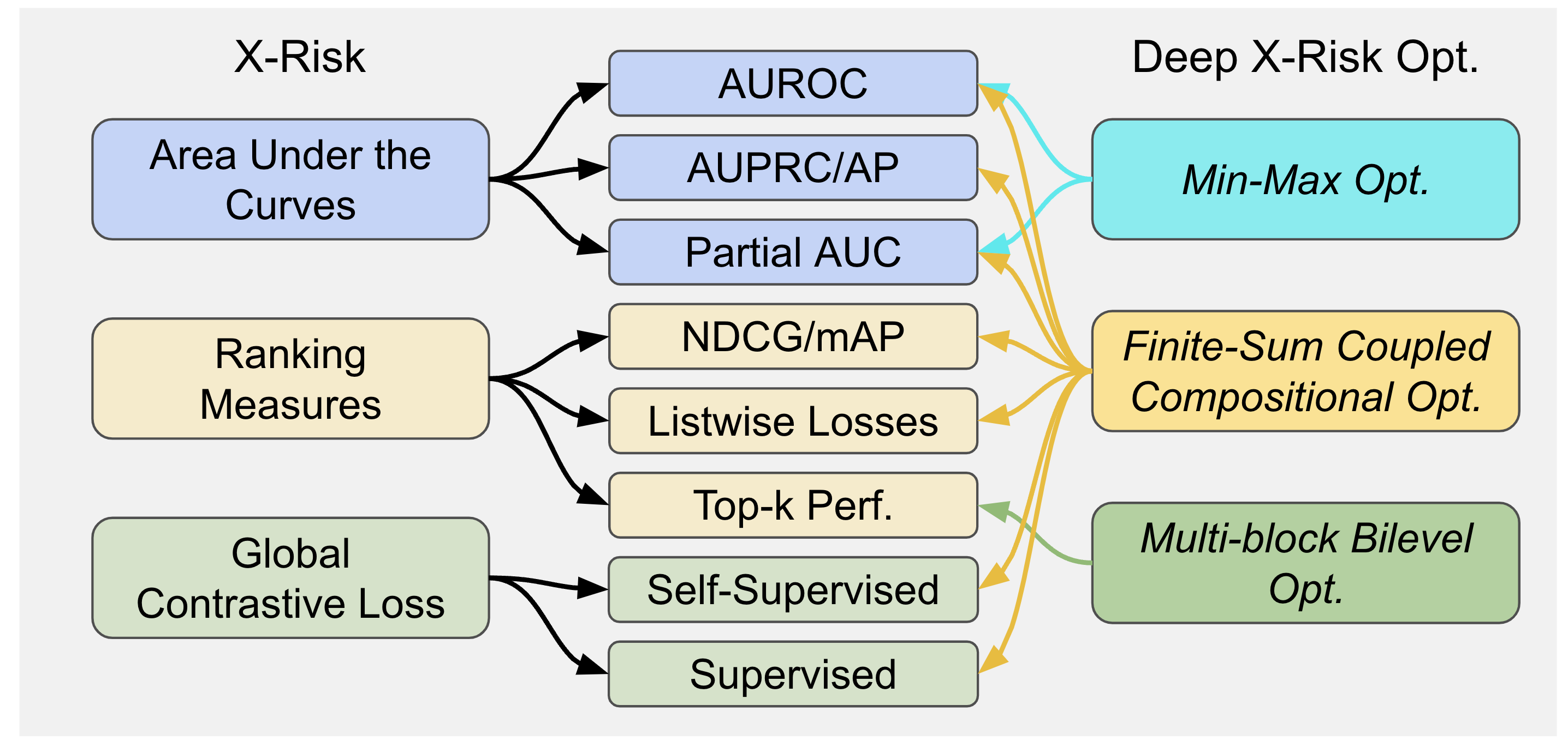
Figure 1. Mappings of X-risks to optimization problems.

Partial Area Under ROC Curve (pAUC) is defined as area under the ROC Curve with a restriction on the range of false positive rate (FPR) and/or true positive rate (TPR). For simplicity, we only consider pAUC with FPR restricted to be less than $\beta\in(0,1]$. Let $\mathcal{S}^{\downarrow}\left[k_{1},k_{2}\right]\subset\mathcal{S}$ be the subset of examples whose rank in terms of their prediction scores in the descending order are in the range of $\left[k_{1},k_{2}\right]$, where $k_{1}\leq k_{2}$. Then, optimizing pAUC with FPR$\leq\beta$ can be cast into:

$$\min_{\mathbf{w}}\frac{1}{n_{+}}\frac{1}{k}\sum\nolimits_{\mathbf{x}_{i}\in\mathcal{S}_{+}}\sum\nolimits_{\mathbf{x}_{j}\in\mathcal{S}^{\downarrow}_{-}[1,k]}\ell(h_{\mathbf{w}}(\mathbf{x}_{j})-h_{\mathbf{w}}(\mathbf{x}_{i})),$$

where $k=\lfloor n_{-}\beta\rfloor$. To tackle challenge of handling $\mathcal{S}^{\downarrow}_{-}[1,k]$ for data selection, we consider the following FCCO formulation (Zhu et al., 2022a):

(3) $$\min_{\mathbf{w}}\frac{1}{n_{+}}\sum\nolimits_{\mathbf{x}_{i}\in\mathcal{S}_{+}}\lambda\log\mathbb{E}_{\mathbf{x}_{j}\in\mathcal{S}_{-}}\exp(\frac{\ell(h_{\mathbf{w}}(\mathbf{x}_{j})-h_{\mathbf{w}}(\mathbf{x}_{i}))}{\lambda}),$$

where $\lambda>0$ is a temperature parameter that plays a similar role of $k$. Let $g(\mathbf{w};\mathbf{x}_{i},\mathcal{S}_{-})=\mathbb{E}_{x_{j}\in\mathcal{S}_{-}}\exp(\ell(h_{\mathbf{w}}(\mathbf{x}_{j})-h_{\mathbf{w}}(\mathbf{x}_{i}))/\lambda)$ and $f_{i}(g)=\lambda\log(g)$. Then (3) is a special case of FCCO. In LibAUC, we have implemented SOPAs for optimizing the above objective of one-way pAUC with FPR$\leq\beta$ and SOTAs for optimizing a similarly formed surrogate loss of two-way pAUC with FRP$\leq\beta$ and TPR$\geq\alpha$ as proposed in (Zhu et al., 2022a).

Area Under Precision-Recall Curve (AUPRC) is an aggregated measure of precision of the model at all recall levels. A non-parametric estimator of AUPRC is Average Precision (AP) (Boyd et al., 2013):

AP $$=\frac{1}{n_{+}}\sum\limits_{\mathbf{x}_{i}\in\mathcal{S}_{+}}\frac{\sum\limits_{\mathbf{x}_{j}\in\mathcal{S}_{+}}\mathbb{I}(h_{\mathbf{w}}(\mathbf{x}_{j})\geq h_{\mathbf{w}}(\mathbf{x}_{i}))}{\sum\limits_{\mathbf{x}_{j}\in\mathcal{S}}\mathbb{I}(h_{\mathbf{w}}(\mathbf{x}_{j})\geq h_{\mathbf{w}}(\mathbf{x}_{i}))}.$$

By using a differentiable surrogate loss $\ell(h_{\mathbf{w}}(\mathbf{x}_{j})-h_{\mathbf{w}}(\mathbf{x}_{i}))$ in place of $\mathbb{I}(h_{\mathbf{w}}(\mathbf{x}_{j})\geq h_{\mathbf{w}}(\mathbf{x}_{i}))$, we consider the following FCCO formulation for AP maximization:

$$\min_{\mathbf{w}}\frac{1}{n_{+}}\sum\limits_{\mathbf{x}_{i}\in\mathcal{S}_{+}}f(g_{1}(\mathbf{w};\mathbf{x}_{i},\mathcal{S}_{+}),g_{2}(\mathbf{w};\mathbf{x}_{i},\mathcal{S})),$$

where $g_{1}(\mathbf{w};\mathbf{x}_{i},\mathcal{S}_{+})=\sum_{\mathbf{x}_{j}\in\mathcal{S}_{+}}\ell(h_{\mathbf{w}}(\mathbf{x}_{j})-h_{\mathbf{w}}(\mathbf{x}_{i}))$, $g_{2}(\mathbf{w};\mathbf{x}_{i},\mathcal{S})=\sum_{\mathbf{x}_{j}\in\mathcal{S}}\ell(h_{\mathbf{w}}(\mathbf{x}_{j})-h_{\mathbf{w}}(\mathbf{x}_{i}))$, and $f(g_{1},g_{2})=-\frac{g_{1}}{g_{2}}$. In LibAUC, we implemented the SOAP algorithm with a momentum SGD or Adam-style update (Qi et al., 2021), which is a special case of SOX analyzed in (Wang and Yang, 2022).

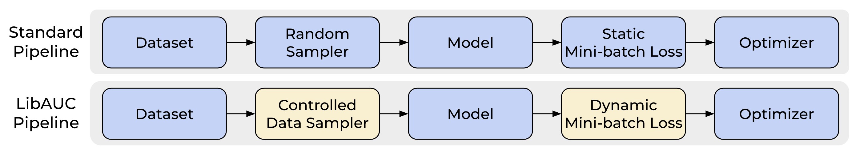
Figure 2. The pipeline of LibAUC modules. Highlighted blocks denote the unique modules of the LibAUC library.

Normalized Discounted Cumulative Gain (NDCG) is a ranking performance metric for LTR tasks. The averaged NDCG over all queries can be expressed by

$$\quad\frac{1}{N}\sum_{q\in\mathcal{Q}}\frac{1}{Z_{q}}\sum_{\mathbf{x}_{i}^{q}\in\mathcal{S}^{+}_{q}}\frac{2^{y^{q}_{i}}-1}{\log_{2}(r(\mathbf{w};\mathbf{x}^{q}_{i},\mathcal{S}_{q})+1)},$$

where $r(\mathbf{w};\mathbf{x},\mathcal{S}_{q})=\sum_{\mathbf{x}^{\prime}\in\mathcal{S}_{q}}\mathbb{I}(h_{\mathbf{w}}(\mathbf{x}^{\prime},q)-h_{\mathbf{w}}(\mathbf{x},q)\geq 0)$ denotes the rank of $\mathbf{x}$ in the set $\mathcal{S}_{q}$ respect to $q$, and $Z_{q}$ is the DCG score of a perfect ranking of items in $\mathcal{S}_{q}$, which can be pre-computed. For optimization, the rank function $r(\mathbf{w};\mathbf{x}_{i}^{q},\mathcal{S}_{q})$ is replaced by a differentiable surrogate loss, e.g., $g(\mathbf{w};\mathbf{x}_{i},\mathcal{S}_{q})=\sum_{\mathbf{x}^{\prime}\in\mathcal{S}_{q}}\ell(h_{\mathbf{w}}(\mathbf{x}^{\prime},q)-h_{\mathbf{w}}(\mathbf{x},q))$. Hence, NDCG optimization is formulated as FCCO. In LibAUC, we implemented the SONG algorithm with a momentum or Adam-style update for NDCG optimization (Qiu et al., 2022), which is a special case of SOX analyzed in (Wang and Yang, 2022).

Top-$K$ NDCG only computes the corresponding score for those that are ranked in the top-$K$ positions. We follow (Qiu et al., 2022) to formulate top-$K$ NDCG optimization as a multi-block bilevel optimization:

$$\min_{\mathbf{w}}-\frac{1}{N}\sum_{q=1}^{N}\frac{1}{Z^{K}_{q}}\sum_{\mathbf{x}_{i}^{q}\in\mathcal{S}^{+}_{q}}\frac{\sigma(h_{q}(\mathbf{x}_{i}^{q};\mathbf{w})-\lambda_{q}(\mathbf{w}))(2^{y^{q}_{i}}-1)}{\log_{2}(g(\mathbf{w};\mathbf{x}^{q}_{i},\mathcal{S}_{q})+1)},$$

$$\lambda_{q}(\mathbf{w})=\arg\min_{\lambda}L(\lambda,\mathbf{w};K,\mathcal{S}_{q}),\forall q\in\mathcal{Q},$$

where $\sigma(\cdot)$ is a sigmoid function, $Z^{K}_{q}$ is the top-$K$ DCG score of a perfect ranking of items, and $\lambda_{q}(\mathbf{w})$ is an approximation of the $(K+1)$-th largest score of data in the set $\mathcal{S}_{q}$. The detailed formulation of lower-level problem $L$ can be found in (Qiu et al., 2022). In LibAUC, we implemented the K-SONG algorithm with a momentum or Adam-style update for top-$K$ NDCG optimization (Qiu et al., 2022).

Listwise CE loss is defined by a cross-entropy loss between two probabilities of list of scores similar to ListNet in (Cao et al., 2007):

(4) $$\min_{\mathbf{w}}-\sum_{q}\sum_{\mathbf{x}^{q}_{i}\in\mathcal{S}_{q}}P(y^{q}_{i})\log\frac{\exp(h_{\mathbf{w}}(\mathbf{x}^{q}_{i};q)}{\sum_{\mathbf{x}\in\mathcal{S}_{q}}\exp(h_{\mathbf{w}}(\mathbf{x}^{q}_{i};q))},$$

where $P(y^{q}_{i})\propto y^{q}_{i}$ denotes a probability for a relevance score $y^{q}_{i}$ to be the top one. (4) is a special case of FCCO by setting $g(\mathbf{w};\mathbf{x}^{q}_{i},\mathcal{S}_{q})=\mathbb{E}_{\mathbf{x}\in\mathcal{S}_{q}}\exp(h_{\mathbf{w}}(\mathbf{x};q)-h_{\mathbf{w}}(\mathbf{x}^{q}_{i};q))$ and $f_{q,i}(g)=P(y^{q}_{i})\log(g)$. In LibAUC, we implemented an optimization algorithm, similar to SONG, for optimizing listwise CE loss.

Global Contrastive Losses (GCL) are the global variants of contrastive losses used for unimodal and bimodal SSL. For unimodal SSL, GCL can be formulated as:

$$\min_{\mathbf{w}}\mathbb{E}_{\mathbf{x}_{i},\mathbf{x}_{i}^{+}}\tau\log\mathbb{E}_{\mathbf{x}_{j}\sim\mathcal{S}_{i}^{-}}\exp\left(\frac{h_{\mathbf{w}}(\mathbf{x}_{i})^{\top}h_{\mathbf{w}}(\mathbf{x}_{j})-h_{\mathbf{w}}(\mathbf{x}_{i})^{\top}h_{\mathbf{w}}(\mathbf{x}_{i}^{+})}{\tau}\right),$$

where $\tau>0$ is a temperature parameter and $\mathbf{x}_{i}^{+}$ denotes a positive data of $\mathbf{x}_{i}$. Different from (Chen et al., 2020; Radford et al., 2021a), GCL use all possible negative samples $\mathcal{S}_{i}^{-}$ for each anchor data instead of mini-batch samples $\mathcal{B}$ (Yuan et al., 2022), which helps address the large-batch training challenge in (Chen et al., 2020). In LibAUC, we implemented an optimization algorithm called SogCLR(Yuan et al., 2022) for optimizing both unimodal/bimodal GCL.

As of June 4, 2023, the LibAUC library has been downloaded 36,000 times. We also implemented two additional algorithms namely MIDAM for solving multi-instance deep AUROC maximization (Zhu et al., 2023) and iSogCLR (Qiu et al., 2023) for optimizing GCL with individualized temperature parameters, which are not studied in this paper.

1 for $t=0,\ldots,T$ do

2       Draw two subsets $\mathcal{B}^{t}_{1}\subset\mathcal{S}_{+}$ and $\mathcal{B}^{t}_{2}\subset\mathcal{S}_{-}$

3       for $i\in\mathcal{B}^{t}_{1}$ do

4             $\mathbf{u}^{t+1}_{i}=(1-\gamma)\mathbf{u}^{t}_{i}+\gamma g_{i}(\mathbf{w}_{t};\mathbf{x}_{i},\mathcal{B}^{t}_{2})$

5             $p_{i}^{t}=\nabla f(\mathbf{u}^{t+1}_{i})=\lambda/\mathbf{u}^{t+1}_{i}$

6       end for

7      Compute the gradient estimator $G_{t}$ by $\frac{1}{|\mathcal{B}^{t}_{1}|}\sum_{\mathbf{x}_{i}\in\mathcal{B}^{t}_{1}}\frac{1}{|\mathcal{B}^{t}_{2}|}\sum_{\mathbf{x}_{j}\in\mathcal{B}^{t}_{2}}p_{i}^{t}\nabla_{\mathbf{w}}\exp(\ell(h_{\mathbf{w}_{t}}(\mathbf{x}_{i}),h_{\mathbf{w}_{t}}(\mathbf{x}_{j}))/\lambda)$

8       Update the model parameter by an optimizer

9      

10 end for

Algorithm 1 SOPAs for solving pAUCLoss.

1 def pAUCLoss(**kwargs): # dynamic mini-batch loss

2   sur_loss = surrogate_loss(neg_logits - pos_logits)

3   exp_loss = torch.exp(sur_loss/Lambda)

4   u[index] = (1 - gamma)*u[index] + gamma*(exp_loss.mean(1))

5   p = (exp_loss/u[index]).detach()

6   loss = torch.mean(p * sur_loss)

7   return loss

8  

9 # optimization

10 for data, targets, index in dataloader:

11   logits = model(data)

12   loss = pAUCLoss(logits, targets, index)

13   optimizer.zero_grad()                     

14   loss.backward()                            

  optimizer.step()

Algorithm 2 High-level pseudocode for SOPAs.

Figure 3. Left: SOPAs for optimizing pAUC; Right: its pseudo code using automatic differentiation of a dynamic mini-batch loss. The corresponding parts of the algorithm and pseudocode are highlighted in the same color.

3. Library Design of LibAUC

The pipeline of training a DL model in the LibAUC library is shown in Figure 2, which consists of five modules, namely Dataset, Data Sampler, Model, Mini-batch Loss, and Optimizer. The Dataset module allows us to get a training sample which includes its input and output. The Data Sampler module provides tools to sample a mini-batch of examples for training at each iteration. The Model module allows us to define different deep models. The Mini-batch Loss module defines a loss function on the selected mini-batch data for backpropagation. The Optimizer module implements methods for updating the model parameter given the computed gradient from backpropagation. While the Dataset, Model, and Optimizer modules are similar to those in existing libraries, the key differences lie in the Mini-batch Loss and Data Sampler modules. The Mini-batch Loss module in LibAUC is referred to as Dynamic Mini-batch Loss, which uses dynamically updated variables to adjust the mini-batch loss. The dynamic variables will be defined in the dynamic mini-batch loss, which can be evaluated by forward propagation. In contrast, we refer to the Mini-batch Loss module in existing libraries as Static Mini-batch Loss, which only uses the sampled data to define a min-batch loss in the same way of the objective but on mini-batch data. TheData Sampler module in LibAUC is referred to as Controled Data Sampler, which differ from standard random data samplers in that the ratio of the number of positive data to the number of negative data can be controlled and tuned to boost the performance. Next, we provide more details of these two and other modules.

3.1. Dynamic Mini-batch Loss

We first present the stochastic gradient estimator of the objective function, which directly motivates our design of Dynamic Mini-batch Loss module.

For simplicity of exposure, we will mainly use the FCCO problem of pAUC optimization (3) to demonstrate the core ideas of the library design. The designs of other algorithms follow in a similar manner. The key challenge is to estimate the gradient using a mini-batch of samples. To motivate the stochastic gradient estimator, we first consider the full gradient given by

$$\nabla F(\mathbf{w})=\mathbb{E}_{\mathbf{x}\in\mathcal{S}_{+}}\nabla f(g(\mathbf{w};\mathbf{x}_{i},\mathcal{S}_{-}))\left(\mathbb{E}_{\mathbf{x}_{j}\in\mathcal{S}_{-}}\nabla\exp(\ell(\mathbf{w};\mathbf{x}_{i},\mathbf{x}_{j})/\lambda)\right).$$

To estimate the full gradient, the outer average over all data in $\mathcal{S}_{+}$ can be estimated by sampling a mini-batch of data $\mathcal{B}_{1}\subset\mathcal{S}_{+}$. Similarly, the average over $\mathbf{x}_{j}\in\mathcal{S}_{-}$ in parentheses can be also estimated by sampling a mini-batch of data $\mathcal{B}_{2}\subset\mathcal{S}_{-}$. A technical issue arises when estimating $g(\mathbf{w};\mathbf{x}_{i},\mathcal{S}_{-})$ inside $f$. A naive mini-batch approach is to simply estimate $g(\mathbf{w};\mathbf{x}_{i},S_{-})$ by using a mini-batch of data in $\mathcal{B}_{2}\subset\mathcal{S}_{-}$, i.e., $g(\mathbf{w};\mathbf{x}_{i},\mathcal{B}_{2})=\frac{1}{|\mathcal{B}_{2}|}\sum_{\mathbf{x}_{j}\in\mathcal{B}_{2}}\exp(\ell(\mathbf{w};\mathbf{x}_{i},\mathbf{x}_{j})/\lambda)$. However, the problem is that the resulting estimator $\nabla f(g(\mathbf{w};\mathbf{x}_{i},\mathcal{B}_{2}))$ is biased due to that $f$ is a non-linear function, whose estimation error will depend on the batch size $|\mathcal{B}_{2}|$. As a result, the algorithm will not converge unless the batch size $|\mathcal{B}_{2}|$ is very large. To address this issue, a moving average estimator is used to estimate $g(\mathbf{w}_{t};\mathbf{x}_{i},\mathcal{S}_{-})$ at the $t$-th iteration (Wang and Yang, 2022; Yuan et al., 2022; Qiu et al., 2022; Qi et al., 2021; Zhu et al., 2022a), which is updated for sampled data $\mathbf{x}_{i}\in\mathcal{B}^{t}_{1}$ according to:

$$\mathbf{u}^{t+1}_{i}=(1-\gamma)\mathbf{u}^{t}_{i}+\gamma g(\mathbf{w}_{t};\mathbf{x}_{i},\mathcal{B}^{t}_{2})$$

$$=(1-\gamma)\mathbf{u}^{t}_{i}+\gamma\frac{1}{|\mathcal{B}^{t}_{2}|}\sum_{\mathbf{x}_{j}\in\mathcal{B}^{t}_{2}}\exp(\ell(h_{\mathbf{w}_{t}}(\mathbf{x}_{j})-h_{\mathbf{w}_{t}}(\mathbf{x}_{i}))/\lambda),$$

where $\gamma\in(0,1)$ is a hyper-parameter. It has been proved that the averaged estimation error of $\mathbf{u}_{i}^{t+1}$ for $g(\mathbf{w}_{t};\mathbf{x}_{i},\mathcal{S}_{-})$ is diminishing in the long run. With the moving average estimators, the gradient of the objective function is estimated by :

$$G_{t}=\mathbb{E}_{\mathbf{x}_{i}\in\mathcal{B}^{t}_{1}}\nabla f({\mathbf{u}^{t+1}_{i}})\nabla g_{i}(\mathbf{w}_{t};\mathbf{x}_{i},\mathcal{B}^{t}_{2})$$

$$=\mathbb{E}_{\mathbf{x}_{i}\in\mathcal{B}^{t}_{1},\mathbf{x}_{j}\in\mathcal{B}^{t}_{2}}\nabla f({\mathbf{u}^{t+1}_{i}})\nabla_{\mathbf{w}}\exp(\ell(h_{\mathbf{w}_{t}}(\mathbf{x}_{j})-h_{\mathbf{w}_{t}}(\mathbf{x}_{i}))/\lambda).$$

The key steps of SOPAs for optimizing pAUC loss are in Algorithm 1 (Zhu et al., 2022a). To facilitate the implementation of computing the gradient estimator $G_{t}$, we design a dynamic mini-batch loss. The motivation of this design is to enable us to simply use the automatic differentiation of PyTorch or TensorFlow for calculating the gradient estimator $G_{t}$. In particular, on PyTorch we aim to define a loss such that we can directly call loss.backward() to compute $G_{t}$. To this end, we define a dynamic variable $p_{i}=\nabla f(\mathbf{u}_{i}^{t+1})$ for $\mathbf{x}_{i}\in\mathcal{B}_{1}^{t}$ and then define a dynamic mini-batch loss as $\texttt{loss}=\frac{1}{|\mathcal{B}_{1}^{t}|}\sum_{\mathbf{x}_{i}\in\mathcal{B}_{1}^{t}}\frac{1}{|\mathcal{B}_{2}^{t}|}\sum_{\mathbf{x}_{j}\in\mathcal{B}_{2}^{t}}p_{i}\exp(\ell(h_{\mathbf{w}_{t}}(\mathbf{x}_{j})-h_{\mathbf{w}_{t}}(\mathbf{x}_{i}))/\lambda)$. However, since $p_{i}$ depends on $\mathbf{u}_{i}^{t+1}$ that is computed based on $\mathbf{w}_{t}$, directly calling loss.backward() for this loss may cause extra differentiation of $p_{i}$ in term of $\mathbf{w}_{t}$. To avoid this, we apply the detach operator p.detach() to separate each $p_{i}$ from the computational graph by returning a new tensor that does not require a gradient. The high-level pseudo code of defining and using the dynamic mini-batch loss for pAUC is given in Algorithm 2, where we use a variable change to define the loss, i.e., $p_{i}=\nabla f(\mathbf{u}_{i}^{t+1})\exp(\ell(h_{\mathbf{w}_{t}}(\mathbf{x}_{j})-h_{\mathbf{w}_{t}}(\mathbf{x}_{i}))/\lambda)/\lambda$.

Below, we give another example of code snippet to implement the dynamic mini-batch contrastive loss for optimizing GCL.

⬇

def GCLoss(**kwargs)

"""Defines dynamic mini-batch loss for GCL."""

# logits: pairwise similarities, labels: pairwise one-hot labels, B: batch size

neg_logits = exp(logits/tau) * (1-labels)

u = (1-gamma) * u[index] \

+ gamma * sum(neg_logits, dim=1)/(2(B-1))

p = (neg_logits/u).detach()

sum_neg_logits = sum(p * logits, dim=1)/(2(B-1))

normalized_logits = logits - sum_neg_logits

loss = -sum(labels * normalized_logits, dim=1)

return loss.mean()

3.2. Controlled Data Sampler

Unlike traditional ERM, DXO requires sampling to estimate the outer average and the inner average. In the example of pAUC optimization by SOPAs, we need to sample two mini-batches $\mathcal{B}^{t}_{1}\subset\mathcal{S}_{+}$ and $\mathcal{B}_{2}^{t}\subset\mathcal{S}_{-}$ at each iteration $t$. We notice that this is common for optimizing areas under curves and ranking measures. For some losses/measures (e.g., AUPRC/AP, NDCG, top-$K$ NDCG, Listwise CE), both sampled positive and negative samples will be used for estimating the inner functions. According to our theoretical analysis (Wang and Yang, 2022), balancing the mini-batch size for outer average and that for the inner average could be beneficial for accelerating convergence. Hence, we design a new Data Sampler module to ensure that both positive and negative samples will be sampled and the proportion of positive samples in the mini-batch can be controlled by a hyper-parameter.

For CID problems, we introduce DualSampler, which takes as input hyper-parameters such as batch_size and sampling_rate, to generate the customized mini-batch samples, where sampling_rate controls the number of positive samples in the mini-batch according to the formula # positives = batch_size*sampling_rate. For LTR problems, we introduce TriSampler, which has hyper-parameters sampled_tasks to control the number of sampled queries for backpropogation, batch_size_per_task to adjust mini-batch size for each query, and sampling_rate_per_task to control the ratio of positives in each mini-batch per query. The TriSampler can be also used for multi-label classification problems with many labels such that sampling labels becomes necessary, which makes the library extendable for our future work.

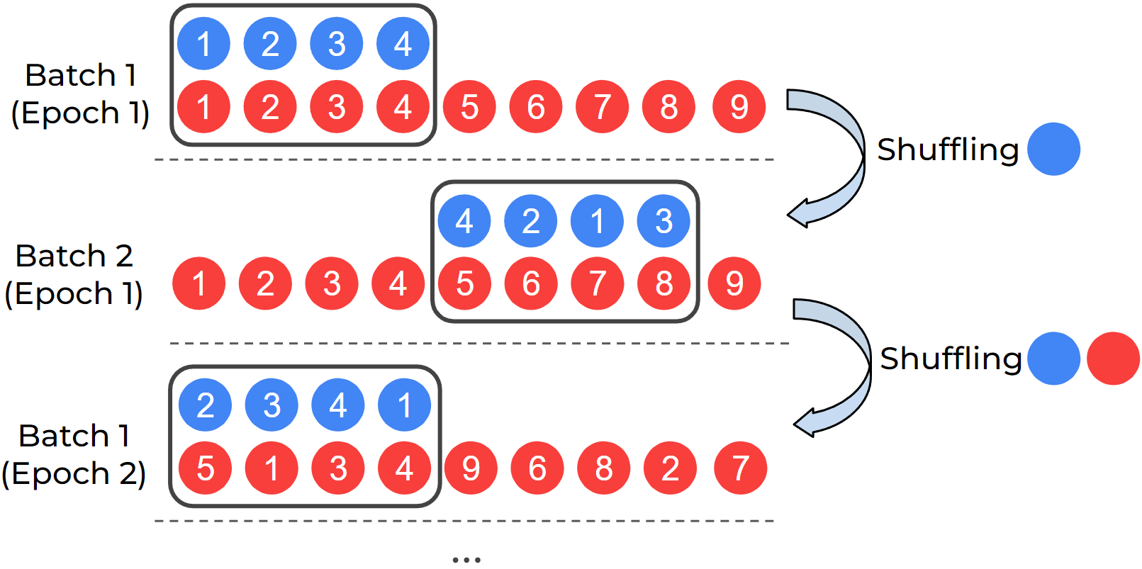
Figure 4. Illustration of DualSampler for an imbalanced dataset with 4 positives $\bullet$ and 9 negatives $\bullet$.

To improve the sampling speed, we have implemented an index-based approach that eliminates the need for computationally intensive operations such as concatenation and append. Figure 4 shows an example of DualSampler for constructing mini-batch data with even positive and negative samples on an imbalanced dataset with 4 positives and 9 negatives. We maintain two lists of indices for the positive data and negative data, respectively. At the beginning, we shuffle the two lists and then take the first 4 positives and 4 negatives to form a mini batch. Once the positive list is used up, we only reshuffle the positive list and take 4 shuffled positives to pair with next 4 negatives in the negative list as a mini-batch. Once the negative list is used up (an “epoch" is done), we re-shuffle both lists and repeat the same process as above. For TriSampler, the main difference is that we first randomly select some queries/labels before sampling the positive and negative data for each query/label. The following code snippet shows how to define DualSampler and TriSampler.

⬇

from libauc.sampler import DualSampler, TriSampler

dualsampler = DualSampler(trainSet,

batch_size=32,

sampling_rate=0.1)

trisampler = TriSampler(trainSet,

batch_size_per_task=32,

sampled_tasks=5,

sampling_rate_per_task=0.1)

3.3. Optimizer

With a calculated gradient estimator, the updating rule for the model parameter of different algorithms for DXO follow similarly as (momentum) SGD or Adam (Wang and Yang, 2022; Zhu et al., 2022a; Qiu et al., 2022; Yuan et al., 2022; Zhu et al., 2022b; Yuan et al., 2021). Hence, the optimizer.step() is essentially the same as that in existing libraries. In addition to our built-in optimizer, users can also utilize other popular optimizers from the PyTorch/TensorFlow library, such as Adagrad, AdamW, RMSprop, and RAdam (Duchi et al., 2011; Loshchilov and Hutter, 2017; Tieleman and Hinton, 2012; Liu et al., 2019a). Hence, we provide an optimizer wrapper that allows users to extend and choose appropriate optimizers. For the naming of the optimizer wrapper, we use the name of optimization algorithms corresponding to each specific X-risk for better code readability. An example of the optimizer wrapper for pAUC optimization is given below, where mode=‘adam’ allows user to use Adam-style update. Another mode is ‘SGD’, which takes a momentum parameter as an argument to use the momentum SGD update.

⬇

#An example of optimizer wrapper.

from libauc.optimizers import SOPAs

optimizer = SOPAs(model.parameters(), lr=0.1, mode=’adam’, weight_decay=1e-4)

3.4. Other Modules

In addition, we provide useful functionalities in other modules, including libauc.datasets, libauc.models, and libauc.metrics, to help users improve their productivity. The libauc.datasets module provides pre-processing functions for several widely-used datasets, including CIFAR (Krizhevsky et al., 2009), CheXpert (Irvin et al., 2019), and MovieLens (Harper and Konstan, 2015), allowing users to easily adapt these datasets for use with LibAUC in benchmarking experiments. It is important to note that the definition of the Dataset class is slightly different from that in existing libraries. An example is given below, where __getitem__ returns a triplet that consists of input data, its label and its corresponding index in the dataset, where the index is returned for accommodating DXO algorithms for updating the $\mathbf{u}^{t+1}_{i}$ estimators. The libauc.models module offers a range of pre-defined models for various tasks, including ResNet(He et al., 2016) and DenseNet(Huang et al., 2017) for classification and NeuMF (He et al., 2017) for recommendation. libauc.metrics module offers evaluation wrappers based on scikit-learn for various metrics, such as AUC, AP, pAUC, and NDCG@K. Moreover, it provides an all-in-one wrapper (shown below) to evaluate multiple metrics simultaneously to improve the production efficiency.

⬇

class ImageDataset(torch.utils.data.Dataset):

"""An example of Dataset class"""

def __init__(self, inputs, targets):

self.inputs = inputs

self.targets = targets

def __len__(self):

return len(self.inputs)

def __getitem__(self, index):

data = self.inputs[index]

target = self.targets[index]

return data, target, index

⬇

#An evaluator wrapper

from libauc.metrics import evaluator

scores = evaluator(pred,true,metrics=[’auc’,’ap’,’pauc’])

3.5. Deployment

Before ending this section, we present a list of different losses, their corresponding data samplers and optimizer wrappers of the LibAUC library in Table 1. Finally, we present an example below of building the pipeline for optimizing pAUC using our designed modules.

Table 1. The list of losses, corresponding samplers and optimizer wrappers in libauc. For a complete list, please refer to the documentation of LibAUC.

Loss Function	Data Sampler	Optimizer Wrapper	Reference
libauc.losses	libauc.sampler	libauc.optimizers
AUCMLoss	DualSampler	PESG	(Yuan et al., 2021)
APLoss	DualSampler	SOAP	(Qi et al., 2021)
pAUCLoss(‘1w’)	DualSampler	SOPAs	(Zhu et al., 2022a)
pAUCLoss(‘2w’)	DualSampler	SOTAs	(Zhu et al., 2022a)
NDCGLoss	TriSampler	SONG	(Qiu et al., 2022)
NDCGLoss(topk=5)	TriSampler	SONG	(Qiu et al., 2022)
ListwiseCELoss	TriSampler	SONG	(Qiu et al., 2022)
GCLoss(‘unimodal’)	RandomSampler	SogCLR	(Yuan et al., 2022)
GCLoss(‘bimodal’)	RandomSampler	SogCLR	(Yuan et al., 2022)

⬇

#A high-level training pipeline for optimizing pAUC.

from libauc.losses import pAUCLoss

from libauc.optimizers import SOPAs

from libauc.sampler import DualSampler

from torch.utils.data import Dataloader

...

dataset = ImageDataset(images, labels)

sampler = DualSampler(dataset,sampling_rate=0.1)

dataloader = DataLoader(dataset, sampler, shuffle=False)

Loss = pAUCLoss(’1w’) # one-way pAUC loss

optimizer = SOPAs()

...

for data, targets, index in dataloader:

logits = model(data)

loss = Loss(logits, targets, index)

optimizer.zero_grad()

loss.backward()

optimizer.step()

4. Experiments

In this section, we provide extensive experiments on three tasks CID, LTR and CLR. Although individual algorithms have been studied in their original papers for individual tasks, our empirical studies serves as complement to prior studies in that (i) ablation studies of the two unique features for all three tasks provide coherent insights of the library for optimizing different X-risks; (ii) comparison with an existing optimization-oriented library TFCO (Cotter et al., 2019; Narasimhan et al., 2019) for optimizing AUPRC is conducted; (iii) a larger scale dataset is used for LTR, and re-implementation of our algorithms for LTR is done on TensorFlow for fair comparison with the TF-Ranking library (Pasumarthi et al., 2019); (iv) evaluation of different DXO algorithms based on different areas under the curves is performed exhibiting useful insights for practical use; (v) larger image-text datasets are used for evaluating SogCLR for bimodal SSL. Another difference from prior works (Qi et al., 2021; Zhu et al., 2022a; Yuan et al., 2021; Qiu et al., 2022) is that all experiments for CID and LTR are conducted in an end-to-end training fashion without using a pretraining strategy. However, we did observe the pretraining generally helps improve performance (cf. the Appendix).

Table 2. Results on three classification tasks. Best results are marked in bold and second-best results are marked in underline.

Methods	CIFAR10 (imratio=1%)			CheXpert (imratio=24.54%)			OGB-HIV (imratio=1.76%)
	AUROC	AP	pAUC (fpr<0.3)	AUROC	AP	pAUC (fpr<0.3)	AUROC	AP	pAUC (fpr<0.3)
CE	0.687±0.008	0.681±0.005	0.619±0.003	0.853±0.006	0.687±0.012	0.769±0.011	0.765±0.002	0.250±0.013	0.721±0.004
Focal	0.678±0.006	0.671±0.009	0.610±0.007	0.879±0.004	0.737±0.010	0.800±0.006	0.758±0.004	0.241±0.009	0.722±0.003
PESG	0.712±0.009	0.706±0.011	0.639±0.009	0.890±0.002	0.759±0.009	0.820±0.003	0.805±0.009	0.199±0.009	0.745±0.007
SOAP	0.711±0.027	0.717±0.016	0. 648±0.013	0.875±0.048	0.757±0.074	0.813±0.059	0.709±0.008	0.293±0.004	0.699±0.001
SOPAs	0.717±0.005	0.713±0.002	0.645±0.003	0.894±0.003	0.767±0.008	0.823+0.006	0.786±0.007	0.249±0.019	0.747±0.004

4.1. Classification for Imbalanced Data

We choose three datasets from different domains, namely CIFAR10 - a natural image dataset  (Krizhevsky et al., 2009), CheXpert - a medical image dataset (Irvin et al., 2019) and OGB-HIV - a molecular graph dataset (Hu et al., 2020). For CIFAR10, we follow the original paper (Yuan et al., 2021) to construct an imbalanced training set with a positive sample ratio (referred as imratio) of 1%. For evaluation, we sample 5% data from training set as validation set and re-train the model using full training set after selecting the parameters and finally report the performance on testing set with balanced positive and negative classes. For CheXpert, we follow the original work (Yuan et al., 2021) by conducting experiments on 5 selected diseases, i.e., Cardiomegaly (imratio=12.2%), Edema (imratio=32.2%), Consolidation (imratio=6.8%), Atelectasis (imratio=31.2%), Pleural Effusion (imratio=40.3%), with an average of imratio of 24.54%. We use the downsized $224\times 224$ frontal images only for training. Due to the unavailability of testing set, we report the averaged results of 5 tasks on the official validation set. For OGB-HIV, the dataset has an imratio of 1.76% and we use official train/valid/test split for experiments and report the final performance on testing set. For each setting, we repeat experiments three times using different random seeds and report the final results in mean$\pm$std.

For modeling, we use ResNet20, DenseNet121, and DeepGCN (He et al., 2016; Huang et al., 2017; Li et al., 2020) for the three datasets, respectively. We consider optimizing three losses, namely AUCMLoss, APLoss, pAUCLoss by using PESG, SOAP, SOPAs, respectively. For the latter two, we use the pairwise squared hinge loss with a margin parameter in their definition. Thus, all losses have a margin parameter, which is tuned in [0.1, 0.3, 0.5, 0.7, 0.9, 1.0]. For APLoss and pAUCLoss, we tune the moving average estimator parameter $\gamma$ in the same range. For pAUCLoss, we also tune the temperature parameter in [0.1, 1.0, 10.0]. For DualSampler, we tune sampling_rate in [0.1, 0.3, 0.5]. For baselines, we compare two popular loss functions used in the literature, i.e., CE loss and Focal loss. For Focal loss, we tune $\hat{\alpha}$ in [1,2,5] and $\hat{\gamma}$ in [0.25, 0.5, 0.75]. For optimization, we use the momentum SGD optimizer for all methods with a default momentum parameter 0.9 and tuned initial learning rate in [0.1, 0.05, 0.01]. We decay learning rate by 10 times at 50% and 75% of total training iterations. For CIFAR10, we run all methods using a batch size of 128 for 100 epochs. For CheXpert, we train models using a batch size of 32 for 2 epochs. For OGB-HIV, we train models using a batch size of 512 for 100 epochs. To evaluate the performance, we adopt three different metrics, i.e., AUROC, AP, and pAUC (FPR<0.3). We select the best configuration based on the performance metric to be optimized, e.g., using AUROC for model selection of AUCMLoss. The results are summarized in the Table 2.

We have several interesting observations. Firstly, directly optimizing performance metrics leads to better performance compared to baseline methods based on ERM framework. For example, PESG, SOAP, and SOPAs outperform CE and Focal Loss by a large margin in all datasets. This is consistent with prior works. Secondly, optimizing a specific metric does not necessarily has the best performance for other metrics. For example, on OGB-HIV dataset PESG has the highest AUROC but the lowest AP score, while SOAP has the highest AP score but lowest AUROC and pAUC, and SOPAs has the highest pAUC score. This confirms the importance of choosing appropriate methods in LibAUC for corresponding metrics. Thirdly, on CheXpert, it seems that optimizing pAUC is more beneficial than optimizing full AUROC. SOPAs achieves better performance than PESG and SOAP in all three metrics.

Comparison with the TFCO library. We compare LibAUC (SOAP) with TFCO (Cotter et al., 2019; Narasimhan et al., 2019) for optimizing AP. We run both methods using batch size of 128 for 100 epochs with Adam optimizer and learning rate of 1e-3 and weight decay of 1e-4 on constructed CIFAR10 with imratio={1%,2%}. We plot the learning curves on training and testing sets in Figure 5. The results indicate that LibAUC consistently performs better than TFCO.

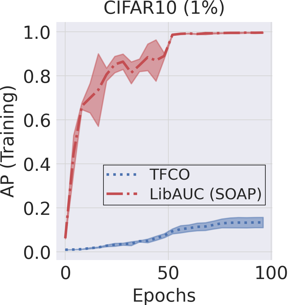
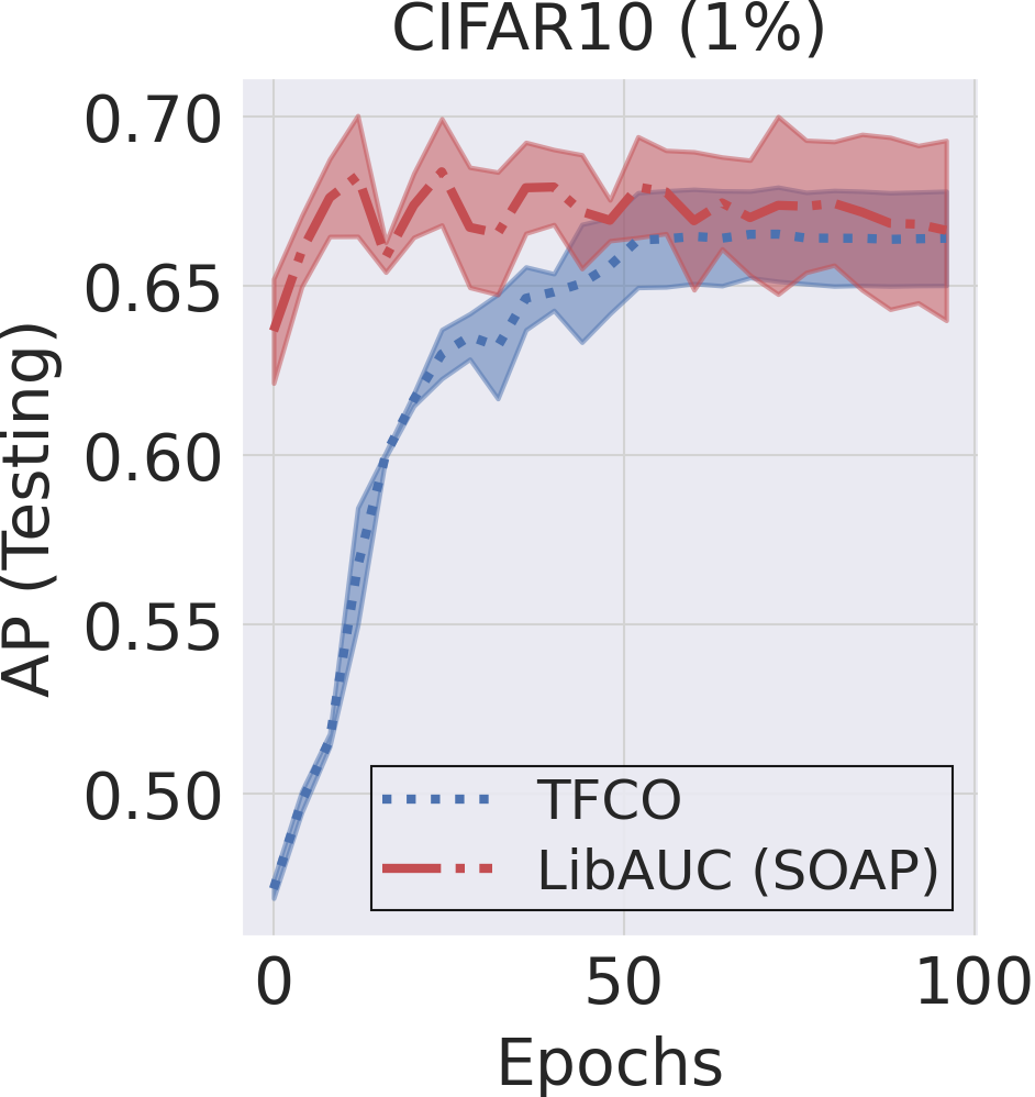
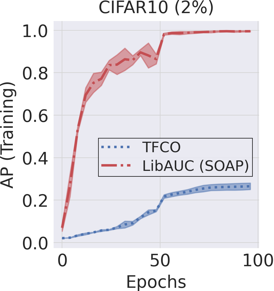
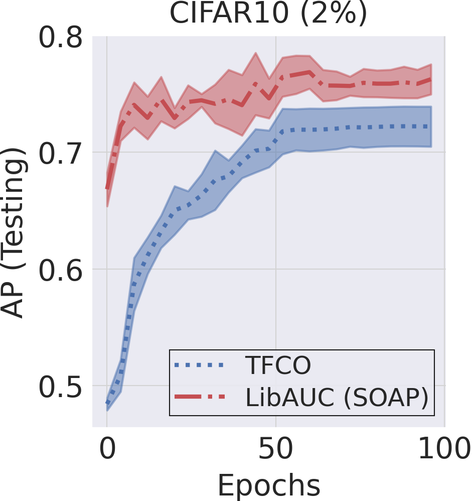
Figure 5. Comparison of TFCO and LibAUC.

Loss	MovieLen20M		MovieLen25M
	NDCG@5	NDCG@20	NDCG@5	NDCG@20
ListMLE (TF-Ranking)	0.2841±0.0007	0.3968±0.0004	0.3771±0.0003	0.4902±0.0003
ApproxNDCG (TF-Ranking)	0.3113±0.0001	0.4362±0.0001	0.3960±0.0003	0.5237±0.0001
GumbelNDCG (TF-Ranking)	0.3179±0.0003	0.4444±0.0001	0.4022±0.0002	0.5285±0.0013
ListwiseCE (LibAUC)	0.3225±0.0005	0.4493±0.0003	0.4104±0.0001	0.5369±0.0001
NDCGLoss(K) (LibAUC)	0.3325±0.0020	0.4497±0.0037	0.4115±0.0008	0.5249±0.0021
NDCGLoss (LibAUC)	0.3476±0.0001	0.4769±0.0003	0.4357±0.0005	0.5614±0.0003

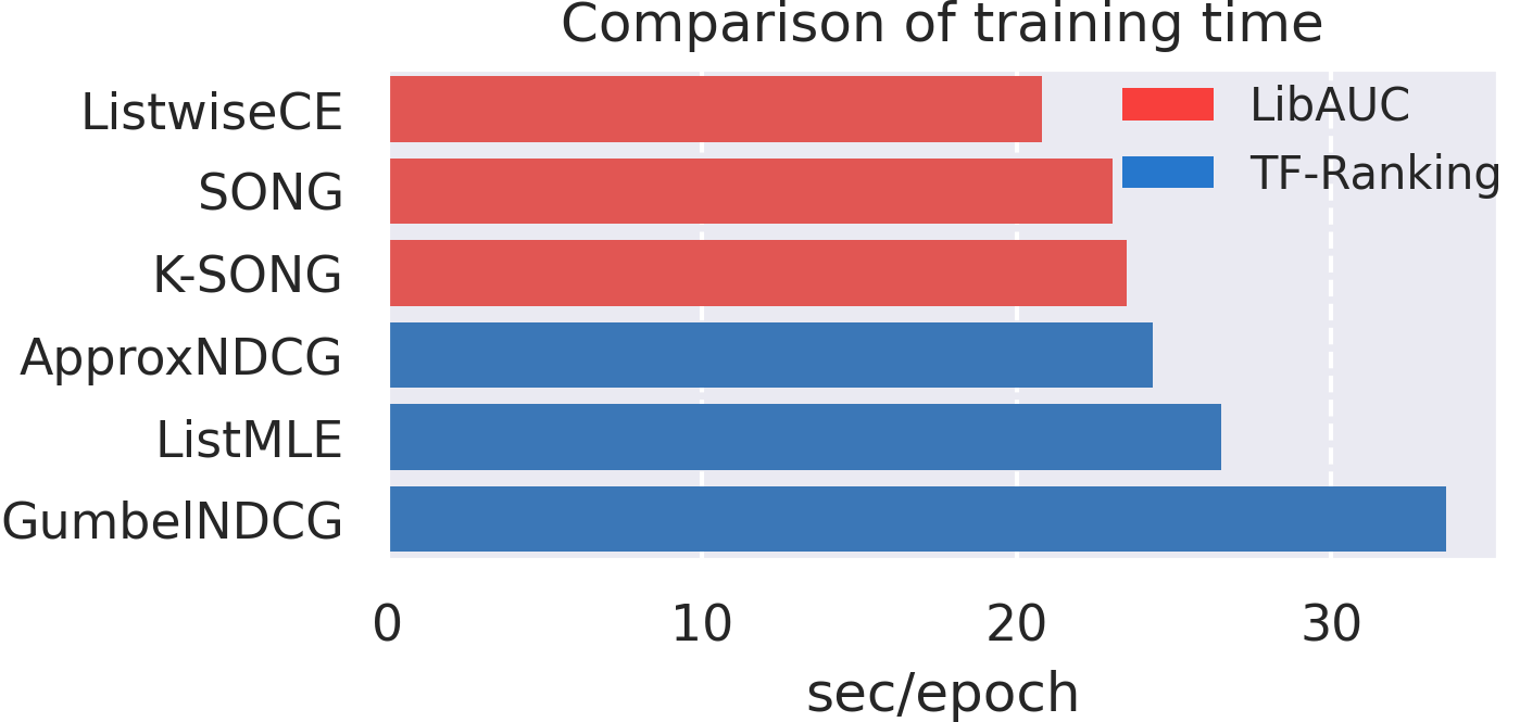
Figure 6. Left: Results on MovieLens datasets. Right: Comparison of training time for LibAUC and TF-Ranking.

4.2. Learning to Rank

We evaluate LibAUC on a LTR task for movie recommendation. The goal is to rank movies for users according to their potential interests of watching based on their historical ratings of movies. We compare the LibAUC library for optimizing ListwiseCELoss, NDCGLoss and top-$K$ NDCG loss denoted by NDCGLoss(K) against the TF-Ranking library (Pasumarthi et al., 2019) for optimizing ApproxNDCG, GumbelNDCG, ListMLE, on two large-scale movie datasets MovieLens20M and MovieLens25M from MovieLens website (Harper and Konstan, 2015). MovieLens20M contains 20 millions movie ratings from 138,493 users and MovieLens25M contains 25 millions movie ratings from 162,541 users. Each user has at least 20 rated movies. Different from (Qiu et al., 2022), we re-implement the SONG and K-SONG (its practical version) on TensorFlow for optimizing the three losses for a fair comparison of running time with TF-Ranking since it is implemented in TensorFlow. To construct training/validation/testing set, we first sort the ratings based on timestamp for each user from oldest to newest. Then, we put 5 most recent ratings in testing set, and the next 5 most recent items in validation set. For training, at each iteration we randomly sample 256 users, and for each user sample 5 positive items from the remaining rated movies and 300 negatives from all unrated movies. For computing validation and testing performance, we sample 1000 negative items from the movie list similar to (Qiu et al., 2022).

For modeling, we use NeuMF (He et al., 2017) as backbone network for all methods. We use the Adam optimizer (Kingma and Ba, 2015) for all methods with an initial learning rate of 0.001 and weight decay of 1e-7 for 120 epochs by following similar settings in (Qiu et al., 2022). During training, we decrease learning rate at 50% and 75% of total iterations by 10 times. For evaluation, we compute and compare NDCG@5 and NDCG@20 for all methods. For NDCGLoss, NDCGLoss(K) and ListwiseCELoss, we tune moving average estimator parameter $\gamma$ in range of [0.1, 0.3, 0.5, 0.7, 0.9, 1.0]. For NDCGLoss(K), we tune $K$ in [50, 100, 300]. We repeat the experiments three times using different random seeds and report the final results in mean$\pm$std. To measure the training efficiency, we conduct the experiments on a NVIDIA V100 GPU and compute the average training times over 10 epochs.

As shown in the Figure 6 (left), LibAUC achieves better performance on both datasets. It is worth mentioning that the results of all methods we reported are generally worse than those reported in (Qiu et al., 2022), likely due to different negative items being used for evaluation. In addition, optimizing NDCGLoss($K$) is not as competitive as optimizing NDCGLoss, which is because that we did not use the pretraining strategy used in (Qiu et al., 2022). In Appendix, we show that using pretraining is helpful for boosting the performance of optimizing NDCGLoss($K$). The runtime comparison, where we report the average runtime in seconds per epoch, is shown in Figure 6 (right). The results show that our implementation of LibAUC on TensorFlow is even faster than three methods in TF-Ranking. It is interesting to note that LibAUC for optimizing ListwiseCE loss is 1.6$\times$ faster than TF-Ranking for optimizing GumbelLoss yet has better performance.

4.3. Contrastive Learning of Representations

In this section, we demonstrate the effectiveness of LibAUC (SogCLR) for optimizing GCLoss on both uimodal and bimodal SSL tasks. For unimodal SSL, we use two scales of the ImageNet dataset: a small subset of ImageNet with 100 randomly selected classes (about 128k images) denoted as ImageNet-100, and the full version of ImageNet (about 1.2 million images) denoted as ImageNet-1000 (Deng et al., 2009). For bimodal SSL, we use MS-COCO and CC3M (Guo et al., 2016; Sharma et al., 2018) for experiments. MS-COCO is a large-scale image recognition dataset containing over 118,000 images and 80 object categories, and each image is associated with 5 captions describing the objects and their interactions in the image. CC3M is a large-scale image captioning dataset that contains almost 3 million image-caption pairs. For evaluation, we compare the feature quality of pretrained encoder on ImageNet-1000 validation set, which consists of 50,000 images that belong to 1000 classes. For unimodal SSL, we conduct linear evaluation by fine-tuning a new classifier in a supervised fashion after pretraining. For bimodal SSL, we conduct zero-shot evaluation by computing similarity scores between the embeddings of the prompt text and images. Due to the high training cost, we only run each experiment once. It is worth noting that the two bimodal datasets were not used in (Yuan et al., 2022).

For unimodal SSL, we follow the same settings in SimCLR (Chen et al., 2020). We use ResNet-50 with a two-layer non-linear head with a hidden size of 128. We use LARS optimizer (You et al., 2017) with an initial learning rate of $0.075\times\sqrt{batch\_size}$ and weight decay of 1e-6. We use a cosine decay strategy to decrease learning rate. We use a batch size of 256 to train ImageNet-1000 for 800 epochs and ImageNet-100 for 400 epochs with a 10-epoch warm-up. For linear evaluation, we train the classifier for additional 90 epochs using the momentum SGD optimizer with no weight decay. For bimodal SSL, we use a transformer (Radford et al., 2019; Vaswani et al., 2017) as the text encoder (cf appendix for structure parameters) and ResNet-50 as the image encoder (Radford et al., 2021a). Similarly, we use LARS optimizer with the same learning rate strategy and weight decay. We use a batch size of 256 for 30 epochs, with a 3-epoch warm-up. For zero-shot evaluation, we compute the accuracy based on the cosine similarities between image embeddings and text embeddings using 80 different prompt templates similar to (Radford et al., 2021a). Note that we randomly sample one out of five text captions to construct text-image pair for pretraining on MS-COCO. We compare SogCLR with SimCLR for unimodal SSL and with CLIP for bimodal SSL tasks. For SogCLR, we tune $\gamma$ in [0.1, 0.3, 0.5, 0.7, 0.8, 0.9, 1.0] and tune temperature $\tau$ in [0.07, 0.1]. All experiments are run on 4-GPU (NVIDIA A40) machines. The results are summarized in Table 3.

Table 3. Results for Self-Supervised Learning. Numbers are denoted in %. SogCLR (Yuan et al., 2022) is re-implemented in PyTorch.

Dataset	Scale	Modality	Acc@1		Acc@5
			SimCLR CLIP	SogCLR	SimCLR CLIP	SogCLR
ImageNet100	0.13M	Image	78.1	80.3	94.9	95.5
ImageNet1000	1.2M	Image	66.5	69.0	87.5	89.2
MS-COCO	0.12M	Image-Text	4.6	5.0	12.2	12.5
CC3M	3M	Image-Text	19.7	21.4	39.3	41.3

The results demonstrate that SogCLR outperforms SimCLR and CLIP for optimizing mini-batch contrastive losses in both tasks. In particular, SogCLR improves 2.2%, 2.9% over SimCLR on ImageNet datasets, and improves 0.5%, 1.6% over CLIP on two bimodal datasets. It is notable that the pretraining for ImageNet lasts up to 800 epochs, while the pretraining on the two bimodal datasets is only performed for 30 epochs due to limited computational resources. According to theorems in (Yuan et al., 2022), the optimization error of SogCLR will diminish as the training epochs increase. We expect that SogCLR exhibit have larger improvements over CLIP with longer epochs.

4.4. Ablation Studies

In this section, we present more ablation studies to demonstrate the effectiveness of our design and superiority of our library.

4.4.1. Effectiveness of Dynamic Mini-batch Losses.

To verify the effectiveness of the dynamic mini-batch losses, we compare them with conventional static mini-batch losses. To this end, we focus on SOAP, SOPAs, SONG and SogCLR, and compare their performance with different values of $\gamma$ in our framework. When setting $\gamma=1$, our algorithms will degrade into their conventional mini-batch versions. We directly use the best hyper-parameters tuned in Section 4.1, 4.2 except for $\gamma$, which is tuned from 0.1 to 1.0. The performance is evaluated using AP (SOAP), pAUC (SOPAs), NDCG@5 (SONG), and Top-1 Accuracy (SogCLR), respectively. The final results of this comparison are summarized in Table 6. Overall, we find that all methods achieve the best performance when $\gamma$ is less than $1$.

4.4.2. Effectiveness of Data Sampler.

We vary the positive sampling rate (denoted as sr) in the DualSampler for CID by optimizing AUCMLoss, and in the TriSampler for LTR by optimizing NDCGLoss. For CID, we use three datasets: CIFAR10 (1%), CheXpert, and OGB-HIV, and tune sr={original, 10%, 30%, 50%}, where sr=original means that we simply use the random data sampler without any control. Other hyper-parameters are fixed to those found as in Section 4.1. The results are evaluated in AUROC and summarized in Table 6. For LTR, we use MovieLens20M dataset. We fix the number of sampled queries (i.e., users) to 256 in each mini-batch and vary the number of positive and negative items, which are tuned in {1, 5, 10} and {1, 5, 10, 100, 300, 500, 1000}, respectively. We fix $\gamma=0.1$ and train the model for 120 epochs with the same learning rate, weight decay and learning rate decaying strategies as in section 4.2. The results are evaluated in NDCG@5 and are shown in Table 6. Both results demonstrate that tuning the positive sampling rate is beneficial for performance improvement.

Table 4. The $\gamma<1$ is better.

Method	Dataset	$\gamma=0.1$	$\gamma=0.3$	$\gamma=0.5$	$\gamma=0.7$	$\gamma=0.9$	$\gamma=1.0$
SOAP	OGB-HIV	0.2745	0.2906	0.2881	0.2930	0.2904	0.2864
SOPAs	OGB-HIV	0.6404	0.7414	0.7413	0.7467	0.7337	0.7383
SONG	MovieLens	0.3476	0.3431	0.3384	0.3339	0.3308	0.3290
SogCLR	ImageNet100	0.8018	0.7956	0.8032	0.7974	0.7994	0.7956
SogCLR	CC3M	0.2138	0.2029	0.1931	0.1873	0.1825	0.1778

Table 5. Tuning the sampling rate is beneficial for AUCMLoss.

Dataset	imratio	sr=original	sr=10%	sr=30%	sr=50%
CIFAR10	1%	0.7071	0.7124	0.7087	0.7110
Cardiomegaly	12.2%	0.8469	0.8515	0.8566	0.8378
Edema	32.2%	0.9341	0.9366	0.9420	0.9337
Consolidation	6.8%	0.8888	0.9096	0.8832	0.8636
Atelectasis	31.9%	0.8231	0.8269	0.8330	0.8353
Pleural Effusion	40.3%	0.9265	0.9258	0.9249	0.9311
OGB-HIV	1.8%	0.7642	0.8054	0.7786	0.7752

Table 6. Tuning the sampling rate is beneficial for NDCGLoss on MovieLens20M.

Pos/Neg	1	5	10	100	300	500	1000
1	0.1315	0.1617	0.1725	0.1972	0.2039	0.2067	0.2078
5	0.1609	0.2289	0.2608	0.3354	0.3480	0.3509	0.3522
10	0.1568	0.2083	0.2374	0.3260	0.3417	0.3472	0.3506

The results reveal that DualSampler largely boosts the performance for AUCMLoss on CIFAR10 and OGB-HIV when sampling rate (sr) is set to 10%. It is interesting to note that balancing the data (sr=50%) did not necessarily improve performance on three cases. However, generally speaking using a sampling ratio higher than the original imbalance ratio is useful. For LTR with TriSampler, we observe a dramatic performance increase when increasing the number of positive samples from 1 to 10, and the number of negative samples from 1 to 300. However, when further increasing the number of negatives from 300 to 1000, the improvement is saturated.

4.4.3. The Impact of Batch Size.

We study the impact of the batch sizes on our methods (SOAP, SOPAs, SONG, SogCLR) using dynamic mini-batch losses and that using static mini-batch losses (i.e., $\gamma=1$). We follow the same experiment settings as in previous section and only vary the batch size. For each batch size, we tune $\gamma$ correspondingly as theories indicate its best value depends on batch size. For SogCLR, we train ResNet50 on ImageNet1000 for 800 epochs using batch sizes in $\{8192,2048,512,128\}$. For SOAP and SOPAs, we train ResNet20 on OGB-HIV for 100 epochs using batch sizes in $\{512,256,128,64\}$. For SONG, we train NeuMF for 120 epochs on MovieLens20M using batch sizes in $\{256,128,64,32\}$. The results are shown in Figure 8, which demonstrates our design is more robust to the mini-batch size.

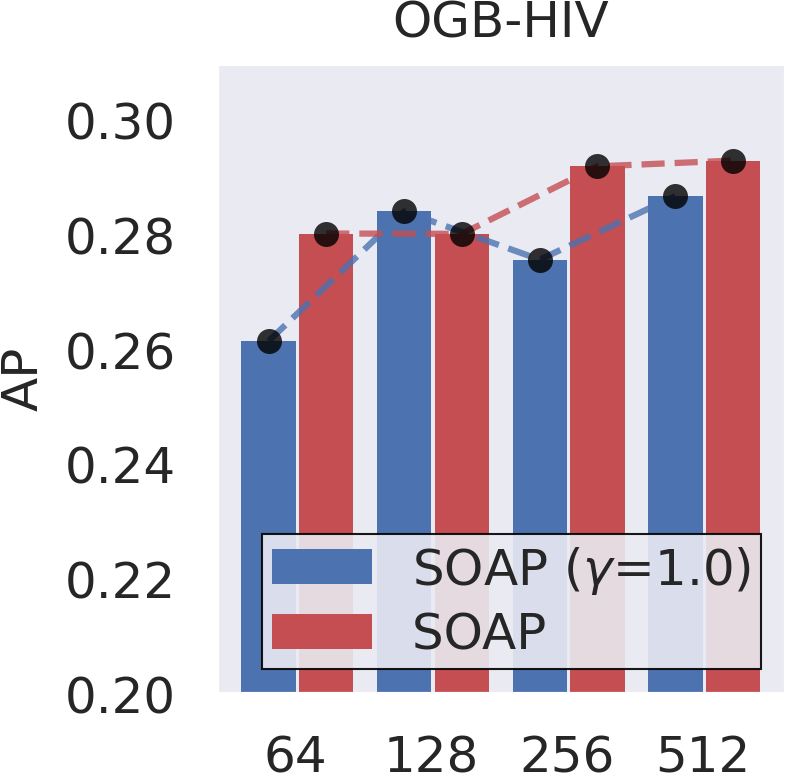
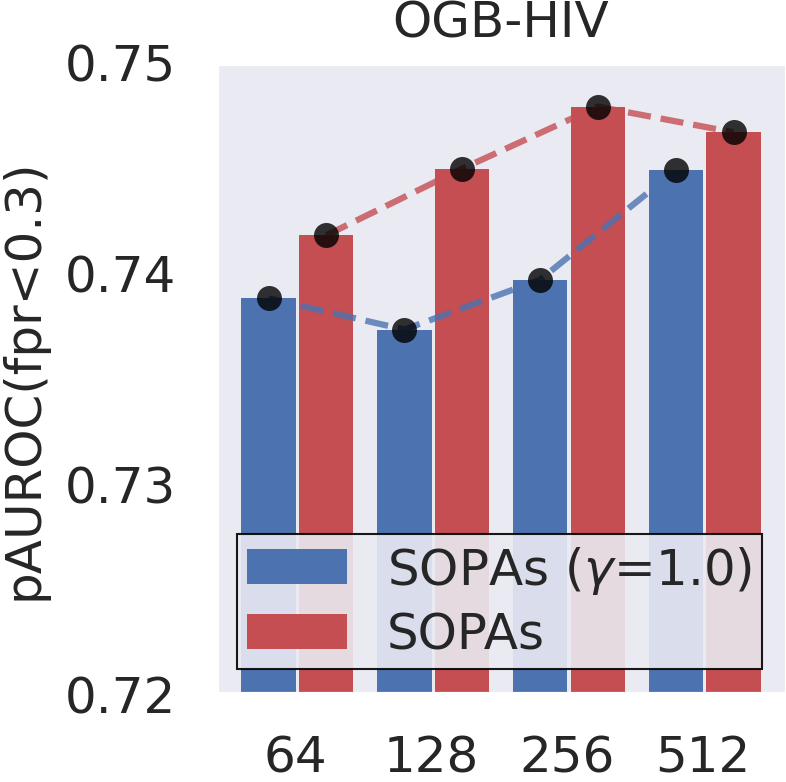
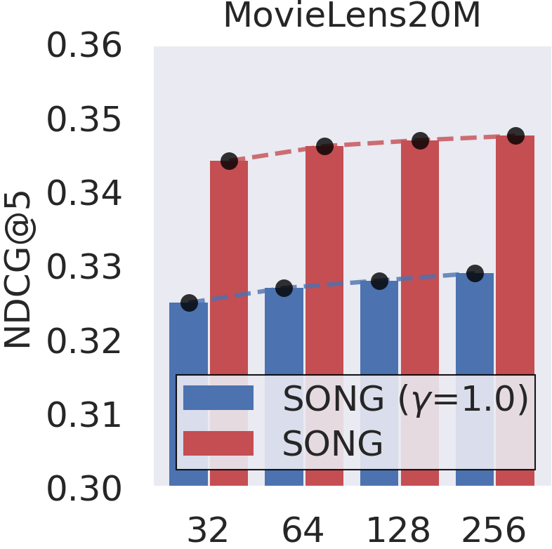
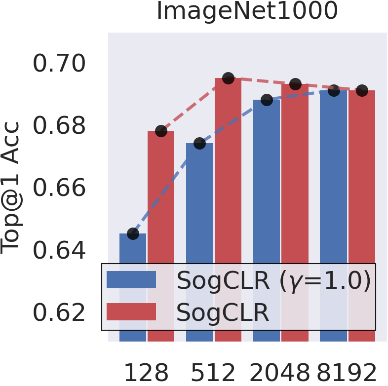
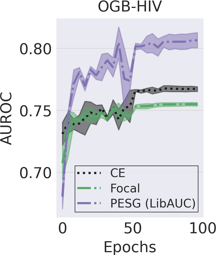
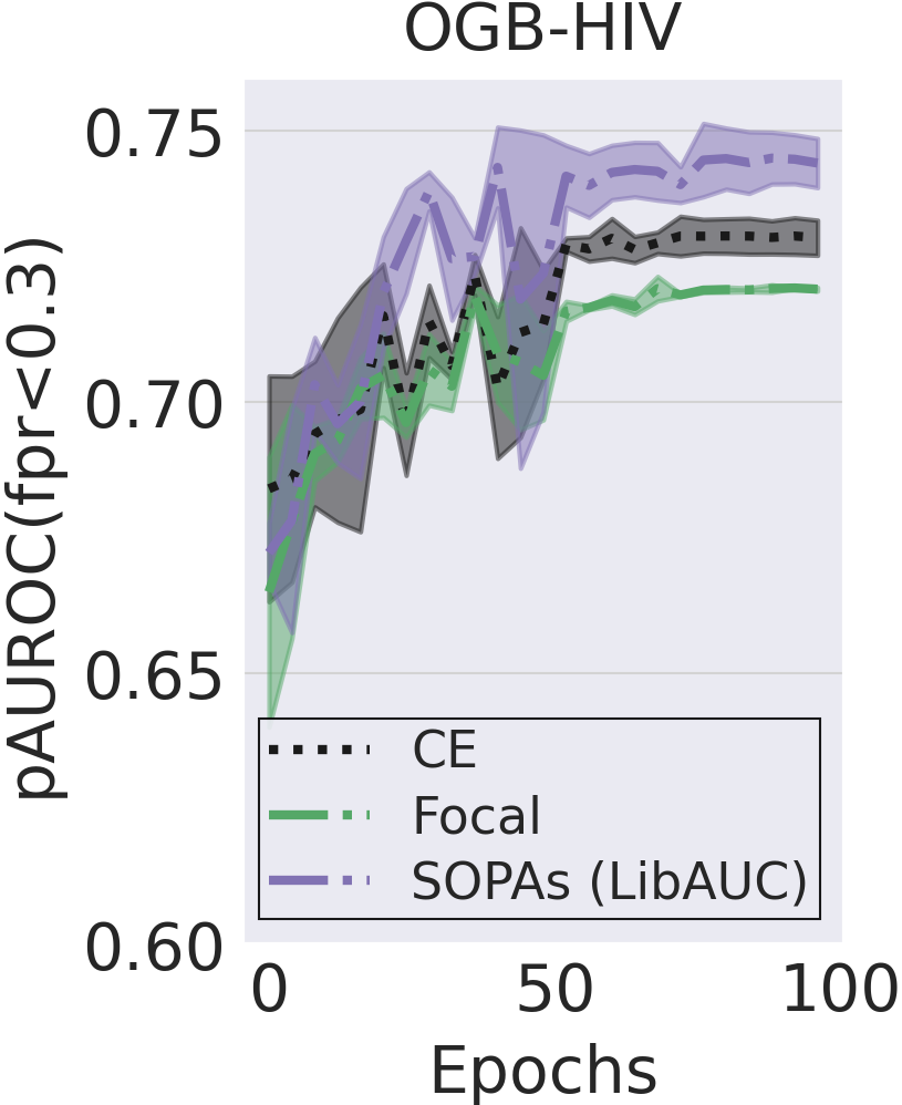
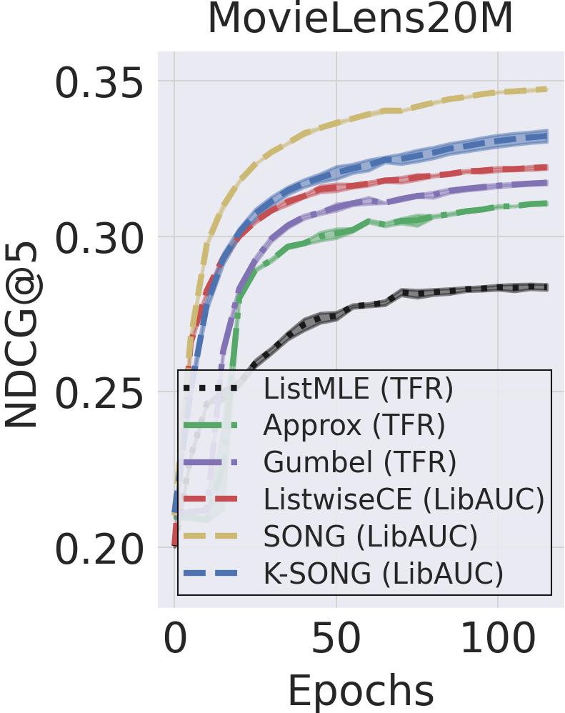
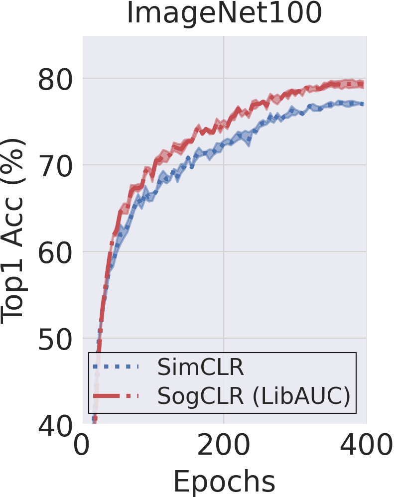
Figure 7. Impact of batch size.

Figure 8. Convergence curves of LibAUC algorithms.

4.4.4. Convergence Speed

Finally, we compare the convergence curves of selected algorithms on the OGB-HIV, MovieLens20M, and ImageNet100 datasets. We use the tuned parameters from previous sections to plot the convergence curves on the testing sets. The results are illustrated in Figure 8. In terms of classification, it is observed that PESG, and SOPAs converge much faster than optimizing CE and Focal loss. For MovieLens20M dataset, we find that SONG has fastest convergence speed compared to all other methods, and K-SONG (without pretraining) is faster than the other baselines but slower than SONG. In the case of SSL, we observe that SogCLR and SimCLR achieve similar performance at the beginning stage, however, SogCLR gradually outperforms SimCLR as the training time goes longer.

5. Conclusion & Future Works

In this paper, we have introduced LibAUC, a deep learning library for X-risk optimization. We presented the design principles of LibAUC and conducted extensive experiments to verify the design principles. Our experiments demonstrate that the LibAUC library is superior to existing libraries/approaches for solving a variety of tasks including classification for imbalanced data, learning to rank, and contrastive learning of representations. Finally, we note that our current implementation of the LibAUC library is by no means exhaustive. In the future, we plan to implement more algorithms for more X-risks, including performance at the top, such as recall at top-$K$ positions, precision at a certain recall level, etc.

Appendix A Appendix

A.1. Pretraining Strategy

We compare the performance of pretraining v.s. random initialization strategy on MovieLens (20M, 25M) with K-SONG and CheXpert with PESG, SOAP, SOPAs, respectively. For K-SONG, we pretrain model using ListwiseCELoss for 30 epochs using learning rate of 0.001 with adam optimizer. Then, we re-initialize last layer and re-train models for 120 epochs by using the tuned parameters in section 4.2. For PESG, SOAP, SOPAs, we use CrossEntropyLoss to pretrain model on CheXpert in multi-label (5 classes) setting for 1 epoch using learning rate of 0.001 with adam optimizer. Then, we re-initialize last layer and re-train models for 2 epochs using the tuned parameters in Section 4.1 for each individual task. We report average scores of five selected diseases in AUC, AP, pAUC. We present the final results in Figure 9. Overall, we can see pretraining boosts the performance of K-SONG by a large margin on two datasets. For CheXpert, we also observe that pretraining can effectively improve the performance on different metrics.

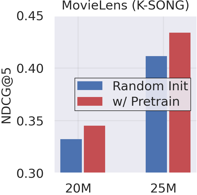
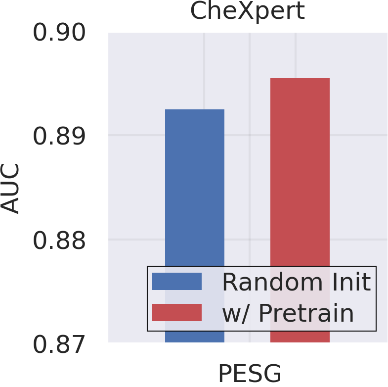
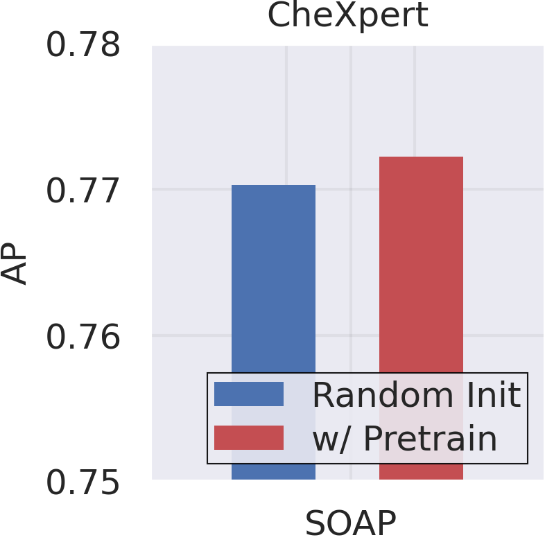
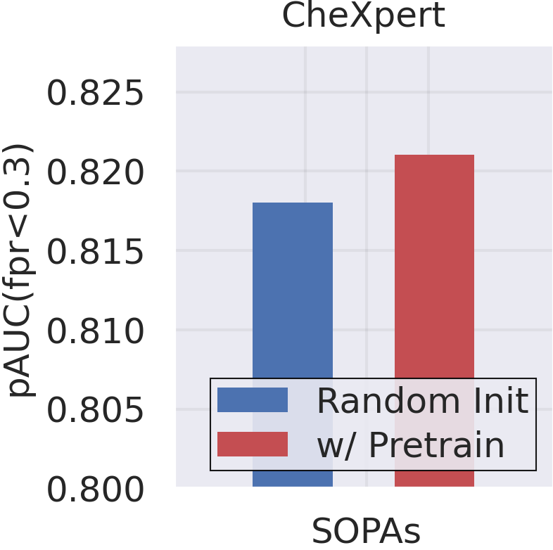
Figure 9. Performance comparison of pretraining v.s. random initialization strategies.

A.2. Relationship between X-Risk Measures

AUROC is a special case of one-way pAUC and two-way pAUC. One-way pAUC with FPR in a range $(0,\alpha)$ is a special case of two-way pAUC. Top Push is a special case of one-way pAUC and p-norm push. AP is a non-parametric estimator of AUPRC. MAP and NDCG are similar in the sense that they are functions of ranks. Top-K MAP, Top-K NDCG, Recall@K (R@K), Precision@K (P@K), pAUC+Precision@K (pAp@K), Precision@Recall (P@R) are similar in the sense that they all involve the computation of K-th largest scores in a set. Listwise losses, supervised contrastive losses, and self-supervised contrastive losses are similar in the sense that they all involve the sum of log-sum term. The above relationships are summarized in Figure 10.

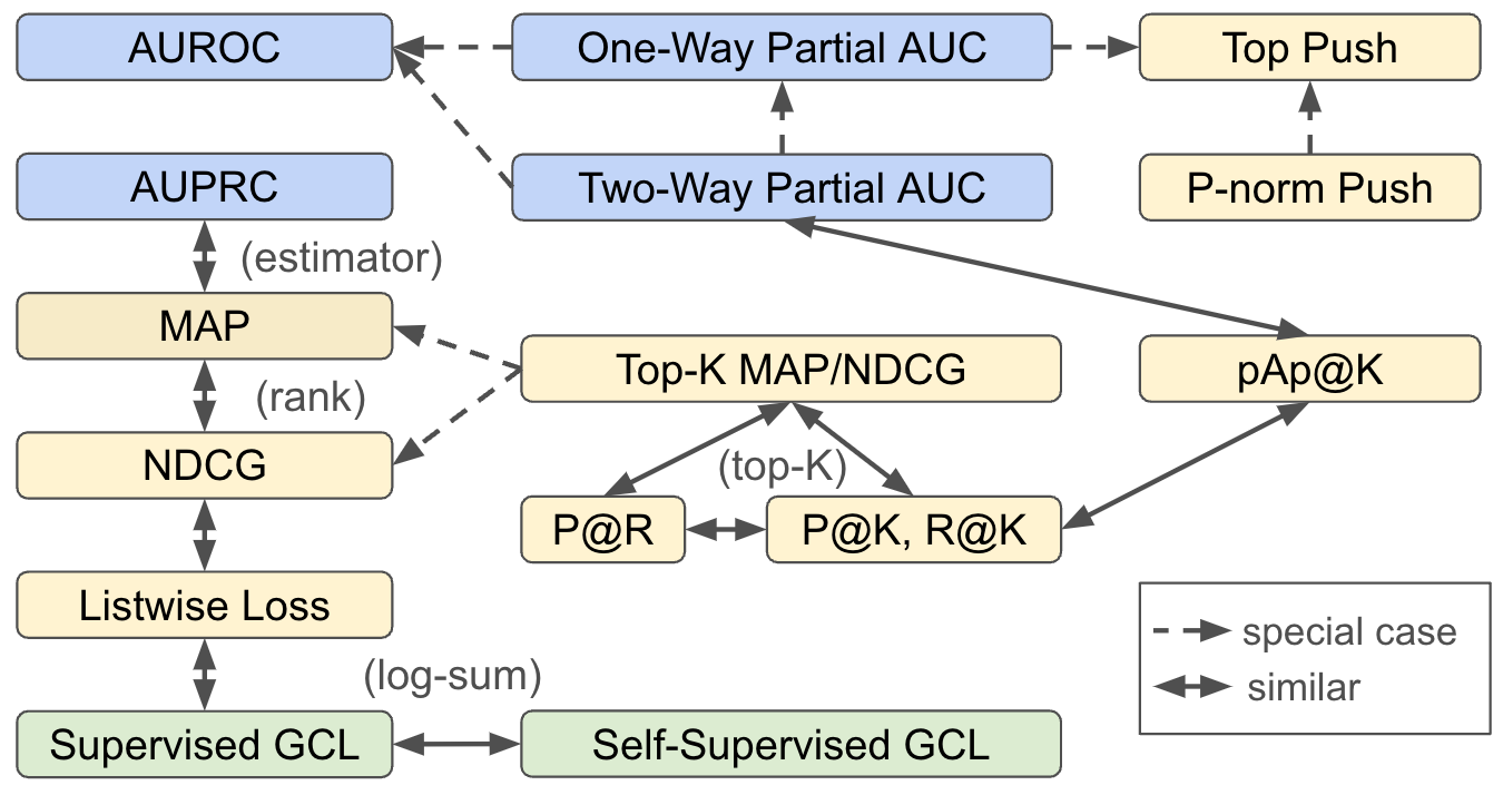
Figure 10. Relationships between different X-risks (Yang, 2022).

A.3. Relationship with Stochastic Compositional Optimization Algorithms

The considered family of problems has a subtle difference from the conventional two level compositional optimization problems studied in the literature (e.g., (Wang et al., 2017b, 2016)), though they are closely related. In traditional two-level compositional optimization, the objective is given by $\mathrm{E}_{\xi}f_{\xi}(\mathrm{E}_{\zeta}g_{\zeta}(\mathbf{w}))$, where the inner random function $g_{\zeta}(\mathbf{w})$ does not depend on the outer random variable $\xi$. Our problem is given by $\frac{1}{n}\sum_{i=1}^{n}f_{i}(g_{i}(\mathbf{w}))$, where $g_{i}(\mathbf{w})=\frac{1}{|\mathcal{S}_{i}|}\sum_{\mathbf{z}_{j}\in\mathcal{S}_{i}}\ell(\mathbf{w},\mathbf{z}_{i},\mathbf{z}_{j})$, which can be written as $\mathrm{E}_{i\sim[n]}[f_{i}(\mathrm{E}_{\mathbf{z}_{j}\sim\mathcal{S}_{i}}\ell(\mathbf{w},\mathbf{z}_{i},\mathbf{z}_{j}))]$. We can see that the key difference between our problem and the conventional two-level compositional optimization problem is that the inner random function $\ell(\mathbf{w},\mathbf{z}_{i},\mathbf{z}_{j})$ in our objective not only depends on the inner random variable $\mathbf{z}_{j}$ but also depends on the outer random variable $\mathbf{z}_{i}$. As a result, we cannot simply apply existing algorithms to solving our problems. Instead, we need to maintain and update estimators for all $g_{i}(\mathbf{w})=\mathrm{E}_{\mathbf{z}_{j}\sim\mathcal{S}_{i}}\ell(\mathbf{w},\mathbf{z}_{i},\mathbf{z}_{j})$ in a random block-wise fashion. Our algorithms were inspired by existing works (e.g., (Wang et al., 2017b, 2016; Ghadimi et al., 2020)), with a key difference in that the moving average estimators for $g_{i}(\mathbf{w})$ are updated only if $\mathbf{z}_{i}$ is in the sampled mini-batch.

A.4. Model Configurations

For the bimodal pretraining experiments in Section 4.3, we implement a small version of CLIP model in PyTorch following the open-source codebase (Ilharco et al., 2021). The model consists of a modified Transformer and ResNet50 (Radford et al., 2019; Vaswani et al., 2017; Radford et al., 2021a). The hyperparameters used for building the model are summarized in Table 7. For the imbalanced classification on OGB-HIV in Section 4.1, we use DeepGCN model (Li et al., 2020), which takes inspiration from the concepts of CNNs, e.g., residual connections. We adapt the DeepGCN codebase on OGB-HIV to our experiments, and the hyperparameters used for building the model are summarized in Table 8.

Table 7. Configuration for CLIP model (Radford et al., 2021a).

Hyperparameter	Value
embed_dim	1024
image_resolution	224$\times$224
vision_layers	[3,4,6,3]
vision_width	32
vision_patch_size	null
context_length	77
vocab_size	49408
transformer_width	512
transformer_heads	8
transformer_layers	12

Table 8. Configuration for DeepGCN model (Li et al., 2020).

Hyperparameter	Value
num_layers	3
embed_dim	256
block	res+
gcn_aggr	max
dropout	0.5
temperature	1.0
norm	batch

A.5. Additional Experiments

We run additional experiments to compare our implemented algorithms with two state-of-the-art baselines: (1) NeuralNDCG for LTR (Pobrotyn and Białobrzeski, 2021), which optimizes NDCG by approximating non-continuous sorting operators based on NeuralSort for LRT tasks, and (2) VICReg for CLR tasks (Bardes et al., 2022), which is based on optimizing invariance, variance, and covariance terms for self-supervised learning of representations.

For VICReg, we pretrain ResNet-50 with a 2-layer non-linear head with a hidden size of 128 on ImageNet100. We follow the same training parameters as stated in Section 4.3. In particular, we pretrain the model for 400 epochs with a batch size of 256, initial learning rate of $0.075\times\sqrt{batch\_size}$, cosine learning rate decay strategy and weight decay of 1e-6. For linear evaluation, we train the classifier for additional 90 epochs using the momentum SGD optimizer with no weight decay. For NeuralNDCG, we train the NeuMF model on MovieLens20M and MovieLens25M datasets. We follow the same training parameters as stated in Section 4.2. In particular, we use the Adam optimizer to train the models with a weight decay of 1e-7 for 120 epochs with the learning rate tuned in the range of [0.001, 0.0005]. For evaluation, we conduct experiments using three different seeds and report the average results in mean±std for NDCG@5 and NDCG@20. The final results for the above two experiments are summarized in Table 9 and Table 10.

Table 9. Comparisons for SSL task on ImageNet100 dataset.

	Acc@1	Acc@5
VICReg	74.3	92.8
SogCLR	80.3	95.5

Table 10. Comparisons for LTR task on MovieLens datasets.

Dataset	Methods	NDCG@5	NDCG@20
MovieLen20M	NeuralNDCG	0.3181±0.0007	0.4424±0.0007
	NDCGLoss (LibAUC)	0.3419±0.0004	0.4709±0.0001
MovieLen25M	NeuralNDCG	0.4059±0.0005	0.5322±0.0006
	NDCGLoss (LibAUC)	0.4295±0.0003	0.5566±0.0005

References

- (1)
- Abadi et al. (2015) Martín Abadi, Ashish Agarwal, Paul Barham, Eugene Brevdo, Zhifeng Chen, Craig Citro, Greg S. Corrado, Andy Davis, Jeffrey Dean, Matthieu Devin, Sanjay Ghemawat, Ian Goodfellow, Andrew Harp, Geoffrey Irving, Michael Isard, Yangqing Jia, Rafal Jozefowicz, Lukasz Kaiser, Manjunath Kudlur, Josh Levenberg, Dandelion Mané, Rajat Monga, Sherry Moore, Derek Murray, Chris Olah, Mike Schuster, Jonathon Shlens, Benoit Steiner, Ilya Sutskever, Kunal Talwar, Paul Tucker, Vincent Vanhoucke, Vijay Vasudevan, Fernanda Viégas, Oriol Vinyals, Pete Warden, Martin Wattenberg, Martin Wicke, Yuan Yu, and Xiaoqiang Zheng. 2015. TensorFlow: Large-Scale Machine Learning on Heterogeneous Systems. https://www.tensorflow.org/ Software available from tensorflow.org.
- Bardes et al. (2022) Adrien Bardes, Jean Ponce, and Yann LeCun. 2022. Vicreg: Variance-invariance-covariance regularization for self-supervised learning. International Conference on Learning Representations (2022).
- Boyd et al. (2013) Kendrick Boyd, Kevin H Eng, and C David Page. 2013. Area under the precision-recall curve: point estimates and confidence intervals. In Joint European conference on machine learning and knowledge discovery in databases. Springer, 451–466.
- Brown et al. (2020) Andrew Brown, Weidi Xie, Vicky Kalogeiton, and Andrew Zisserman. 2020. Smooth-ap: Smoothing the path towards large-scale image retrieval. In Computer Vision–ECCV 2020: 16th European Conference, Glasgow, UK, August 23–28, 2020, Proceedings, Part IX 16. Springer, 677–694.
- Cakir et al. (2019) Fatih Cakir, Kun He, Xide Xia, Brian Kulis, and Stan Sclaroff. 2019. Deep Metric Learning to Rank. In Proceedings of the IEEE/CVF Conference on Computer Vision and Pattern Recognition (CVPR).
- Cao et al. (2007) Zhe Cao, Tao Qin, Tie-Yan Liu, Ming-Feng Tsai, and Hang Li. 2007. Learning to rank: from pairwise approach to listwise approach. In Proceedings of the 24th international conference on Machine learning. 129–136.
- Chen et al. (2020) Ting Chen, Simon Kornblith, Mohammad Norouzi, and Geoffrey Hinton. 2020. A simple framework for contrastive learning of visual representations. In International conference on machine learning. PMLR, 1597–1607.
- cheng Hsieh (2022) Chih cheng Hsieh. 2022. Multimodal-XAI-Medical-Diagnosis-System. https://github.com/ChihchengHsieh/Multimodal-Medical-Diagnosis-System
- Cotter et al. (2019) Andrew Cotter, Heinrich Jiang, and Karthik Sridharan. 2019. Two-player games for efficient non-convex constrained optimization. In Algorithmic Learning Theory. PMLR, 300–332.
- Dang Nguyen et al. (2022) Ngoc Dang Nguyen, Wei Tan, Wray Buntine, Richard Beare, Changyou Chen, and Lan Du. 2022. AUC Maximization for Low-Resource Named Entity Recognition. arXiv e-prints (2022), arXiv–2212.
- Deng et al. (2009) Jia Deng, Wei Dong, Richard Socher, Li-Jia Li, Kai Li, and Li Fei-Fei. 2009. Imagenet: A large-scale hierarchical image database. In 2009 IEEE conference on computer vision and pattern recognition. Ieee, 248–255.
- Duchi et al. (2011) John Duchi, Elad Hazan, and Yoram Singer. 2011. Adaptive subgradient methods for online learning and stochastic optimization. Journal of Machine Learning Research 12, Jul (2011), 2121–2159.
- Garden (2020) TensorFlow Model Garden. 2020. GitHub.
- Ghadimi et al. (2020) Saeed Ghadimi, Andrzej Ruszczynski, and Mengdi Wang. 2020. A single timescale stochastic approximation method for nested stochastic optimization. SIAM Journal on Optimization 30, 1 (2020), 960–979.
- Goyal et al. (2021) Priya Goyal, Quentin Duval, Jeremy Reizenstein, Matthew Leavitt, Min Xu, Benjamin Lefaudeux, Mannat Singh, Vinicius Reis, Mathilde Caron, Piotr Bojanowski, Armand Joulin, and Ishan Misra. 2021. VISSL. https://github.com/facebookresearch/vissl.
- Guo et al. (2016) Yandong Guo, Lei Zhang, Yuxiao Hu, Xiaodong He, and Jianfeng Gao. 2016. Ms-celeb-1m: A dataset and benchmark for large-scale face recognition. In European conference on computer vision. Springer, 87–102.
- Harper and Konstan (2015) F Maxwell Harper and Joseph A Konstan. 2015. The movielens datasets: History and context. Acm transactions on interactive intelligent systems (tiis) 5, 4 (2015), 1–19.
- He et al. (2016) Kaiming He, Xiangyu Zhang, Shaoqing Ren, and Jian Sun. 2016. Deep residual learning for image recognition. In Proceedings of the IEEE conference on computer vision and pattern recognition. 770–778.
- He et al. (2022) Siyuan He, PENGCHENG XI, Ashkan Ebadi, Stéphane Tremblay, and Alexander Wong. 2022. Performance or Trust? Why Not Both. Deep AUC Maximization with Self-Supervised Learning for COVID-19 Chest X-ray Classifications. Journal of Computational Vision and Imaging Systems 7, 1 (Apr. 2022), 37–39. https://doi.org/10.15353/jcvis.v7i1.4906
- He et al. (2017) Xiangnan He, Lizi Liao, Hanwang Zhang, Liqiang Nie, Xia Hu, and Tat-Seng Chua. 2017. Neural collaborative filtering. In Proceedings of the 26th international conference on world wide web. 173–182.
- Hu et al. (2020) Weihua Hu, Matthias Fey, Marinka Zitnik, Yuxiao Dong, Hongyu Ren, Bowen Liu, Michele Catasta, and Jure Leskovec. 2020. Open graph benchmark: Datasets for machine learning on graphs. Advances in neural information processing systems 33 (2020), 22118–22133.
- Huang et al. (2017) Gao Huang, Zhuang Liu, Laurens van der Maaten, and Kilian Q. Weinberger. 2017. Densely Connected Convolutional Networks. In 2017 IEEE Conference on Computer Vision and Pattern Recognition (CVPR). 2261–2269.
- Huang et al. (2022) Mengda Huang, Yang Liu, Xiang Ao, Kuan Li, Jianfeng Chi, Jinghua Feng, Hao Yang, and Qing He. 2022. AUC-Oriented Graph Neural Network for Fraud Detection. In Proceedings of the ACM Web Conference 2022 (Virtual Event, Lyon, France) (WWW ’22). Association for Computing Machinery, New York, NY, USA, 1311–1321. https://doi.org/10.1145/3485447.3512178
- Ilharco et al. (2021) Gabriel Ilharco, Mitchell Wortsman, Nicholas Carlini, Rohan Taori, Achal Dave, Vaishaal Shankar, Hongseok Namkoong, John Miller, Hannaneh Hajishirzi, Ali Farhadi, and Ludwig Schmidt. 2021. OpenCLIP. https://doi.org/10.5281/zenodo.5143773 If you use this software, please cite it as below..
- Irvin et al. (2019) Jeremy Irvin, Pranav Rajpurkar, Michael Ko, Yifan Yu, Silviana Ciurea-Ilcus, Chris Chute, Henrik Marklund, Behzad Haghgoo, Robyn Ball, Katie Shpanskaya, et al. 2019. Chexpert: A large chest radiograph dataset with uncertainty labels and expert comparison. In Proceedings of the AAAI Conference on Artificial Intelligence, Vol. 33. 590–597.
- Jiang et al. (2022) Wei Jiang, Gang Li, Yibo Wang, Lijun Zhang, and Tianbao Yang. 2022. Multi-block-Single-probe Variance Reduced Estimator for Coupled Compositional Optimization. In NeurIPS. http://papers.nips.cc/paper_files/paper/2022/hash/d13ee73683fd5567e5c07634a25cd7b8-Abstract-Conference.html
- Kingma and Ba (2015) Diederik Kingma and Jimmy Ba. 2015. Adam: A method for stochastic optimization. In 3rd International Conference on Learning Representations (ICLR).
- Krizhevsky et al. (2009) Alex Krizhevsky, Geoffrey Hinton, et al. 2009. Learning multiple layers of features from tiny images. (2009).
- Li et al. (2020) Guohao Li, Chenxin Xiong, Ali Thabet, and Bernard Ghanem. 2020. Deepergcn: All you need to train deeper gcns. arXiv preprint arXiv:2006.07739 (2020).
- Liu et al. (2019a) Liyuan Liu, Haoming Wang, Zhenguo Peng, Xiaodong Liu, Xiaohan Chen, Ji Liu, and Jiawei Han. 2019a. On the Variance of the Adaptive Learning Rate and Beyond. arXiv preprint arXiv:1908.03265 (2019).
- Liu et al. (2021) Meng Liu, Youzhi Luo, Limei Wang, Yaochen Xie, Hao Yuan, Shurui Gui, Haiyang Yu, Zhao Xu, Jingtun Zhang, Yi Liu, Keqiang Yan, Haoran Liu, Cong Fu, Bora M Oztekin, Xuan Zhang, and Shuiwang Ji. 2021. DIG: A Turnkey Library for Diving into Graph Deep Learning Research. Journal of Machine Learning Research 22, 240 (2021), 1–9. http://jmlr.org/papers/v22/21-0343.html
- Liu et al. (2019b) Mingrui Liu, Zhuoning Yuan, Yiming Ying, and Tianbao Yang. 2019b. Stochastic auc maximization with deep neural networks. arXiv preprint arXiv:1908.10831 (2019).
- Loshchilov and Hutter (2017) Ilya Loshchilov and Frank Hutter. 2017. Decoupled weight decay regularization. arXiv preprint arXiv:1711.05101 (2017).
- Narasimhan et al. (2019) Harikrishna Narasimhan, Andrew Cotter, and Maya Gupta. 2019. Optimizing generalized rate metrics with three players. Advances in Neural Information Processing Systems 32 (2019).
- Pasumarthi et al. (2019) Rama Kumar Pasumarthi, Sebastian Bruch, Xuanhui Wang, Cheng Li, Michael Bendersky, Marc Najork, Jan Pfeifer, Nadav Golbandi, Rohan Anil, and Stephan Wolf. 2019. Tf-ranking: Scalable tensorflow library for learning-to-rank. In Proceedings of the 25th ACM SIGKDD International Conference on Knowledge Discovery & Data Mining. 2970–2978.
- Paszke et al. (2019) Adam Paszke, Sam Gross, Francisco Massa, Adam Lerer, James Bradbury, Gregory Chanan, Trevor Killeen, Zeming Lin, Natalia Gimelshein, Luca Antiga, et al. 2019. Pytorch: An imperative style, high-performance deep learning library. Advances in neural information processing systems 32 (2019).
- Patel et al. (2022) Yash Patel, Giorgos Tolias, and Jiri Matas. 2022. Recall@k Surrogate Loss with Large Batches and Similarity Mixup. In IEEE Conference on Computer Vision and Pattern Recognition, CVPR. arXiv:2108.11179 https://arxiv.org/abs/2108.11179
- Pobrotyn and Białobrzeski (2021) Przemysław Pobrotyn and Radosław Białobrzeski. 2021. Neuralndcg: Direct optimisation of a ranking metric via differentiable relaxation of sorting. arXiv preprint arXiv:2102.07831 (2021).
- Qi et al. (2021) Qi Qi, Youzhi Luo, Zhao Xu, Shuiwang Ji, and Tianbao Yang. 2021. Stochastic Optimization of Areas Under Precision-Recall Curves with Provable Convergence. Advances in Neural Information Processing Systems 34 (2021).
- Qiu et al. (2023) Zi-Hao Qiu, Quanqi Hu, Zhuoning Yuan, Denny Zhou, Lijun Zhang, and Tianbao Yang. 2023. Not All Semantics are Created Equal: Contrastive Self-supervised Learning with Automatic Temperature Individualization. In Proceedings of International Conference on Machine Learning, Vol. abs/2305.11965. https://doi.org/10.48550/arXiv.2305.11965 arXiv:2305.11965
- Qiu et al. (2022) Zi-Hao Qiu, Quanqi Hu, Yongjian Zhong, Lijun Zhang, and Tianbao Yang. 2022. Large-scale Stochastic Optimization of NDCG Surrogates for Deep Learning with Provable Convergence. In Proceedings of International Conference of Machine Learning. arXiv:2202.12183 [cs.LG]
- Radford et al. (2021a) Alec Radford, Jong Wook Kim, Chris Hallacy, Aditya Ramesh, Gabriel Goh, Sandhini Agarwal, Girish Sastry, Amanda Askell, Pamela Mishkin, Jack Clark, et al. 2021a. Learning transferable visual models from natural language supervision. arXiv preprint arXiv:2103.00020 (2021).
- Radford et al. (2021b) Alec Radford, Jong Wook Kim, Chris Hallacy, Aditya Ramesh, Gabriel Goh, Sandhini Agarwal, Girish Sastry, Amanda Askell, Pamela Mishkin, Jack Clark, Gretchen Krueger, and Ilya Sutskever. 2021b. Learning Transferable Visual Models From Natural Language Supervision. In Proceedings of the 38th International Conference on Machine Learning, ICML 2021, 18-24 July 2021, Virtual Event (Proceedings of Machine Learning Research, Vol. 139), Marina Meila and Tong Zhang (Eds.). PMLR, 8748–8763. http://proceedings.mlr.press/v139/radford21a.html
- Radford et al. (2019) Alec Radford, Jeffrey Wu, Rewon Child, David Luan, Dario Amodei, Ilya Sutskever, et al. 2019. Language models are unsupervised multitask learners. OpenAI blog 1, 8 (2019), 9.
- Research (2021) Tencent Youtu Research. 2021. Heterogeneous interpolation on graph. https://github.com/TencentYoutuResearch/HIG-GraphClassification
- Rolinek et al. (2020) Michal Rolinek, Vit Musil, Anselm Paulus, Marin Vlastelica, Claudio Michaelis, and Georg Martius. 2020. Optimizing Rank-Based Metrics With Blackbox Differentiation. In Proceedings of the IEEE/CVF Conference on Computer Vision and Pattern Recognition (CVPR).
- Sharma et al. (2018) Piyush Sharma, Nan Ding, Sebastian Goodman, and Radu Soricut. 2018. Conceptual captions: A cleaned, hypernymed, image alt-text dataset for automatic image captioning. In Proceedings of the 56th Annual Meeting of the Association for Computational Linguistics (Volume 1: Long Papers). 2556–2565.
- Tieleman and Hinton (2012) Tijmen Tieleman and Geoffrey Hinton. 2012. Lecture 6.5-rmsprop: Divide the gradient by a running average of its recent magnitude. COURSERA: Neural networks for machine learning (2012).
- Vaswani et al. (2017) Ashish Vaswani, Noam Shazeer, Niki Parmar, Jakob Uszkoreit, Llion Jones, Aidan N Gomez, Łukasz Kaiser, and Illia Polosukhin. 2017. Attention is all you need. Advances in neural information processing systems 30 (2017).
- Wang and Yang (2022) Bokun Wang and Tianbao Yang. 2022. Finite-Sum Coupled Compositional Stochastic Optimization: Theory and Applications. In Proceedings of the 39th International Conference on Machine Learning (Proceedings of Machine Learning Research, Vol. 162), Kamalika Chaudhuri, Stefanie Jegelka, Le Song, Csaba Szepesvari, Gang Niu, and Sivan Sabato (Eds.). PMLR, 23292–23317. https://proceedings.mlr.press/v162/wang22ak.html
- Wang et al. (2022) Guanghui Wang, Ming Yang, Lijun Zhang, and Tianbao Yang. 2022. Momentum Accelerates the Convergence of Stochastic AUPRC Maximization. In International Conference on Artificial Intelligence and Statistics, AISTATS 2022, 28-30 March 2022, Virtual Event (Proceedings of Machine Learning Research, Vol. 151), Gustau Camps-Valls, Francisco J. R. Ruiz, and Isabel Valera (Eds.). PMLR, 3753–3771. https://proceedings.mlr.press/v151/wang22b.html
- Wang et al. (2017a) Mengdi Wang, Ethan X Fang, and Han Liu. 2017a. Stochastic compositional gradient descent: algorithms for minimizing compositions of expected-value functions. Mathematical Programming 161, 1-2 (2017), 419–449.
- Wang et al. (2017b) Mengdi Wang, Ethan X Fang, and Han Liu. 2017b. Stochastic compositional gradient descent: algorithms for minimizing compositions of expected-value functions. Mathematical Programming 161, 1-2 (2017), 419–449.
- Wang et al. (2016) Mengdi Wang, Ji Liu, and Ethan Fang. 2016. Accelerating stochastic composition optimization. Advances in Neural Information Processing Systems 29 (2016).
- Wang et al. (2019) Minjie Wang, Da Zheng, Zihao Ye, Quan Gan, Mufei Li, Xiang Song, Jinjing Zhou, Chao Ma, Lingfan Yu, Yu Gai, Tianjun Xiao, Tong He, George Karypis, Jinyang Li, and Zheng Zhang. 2019. Deep Graph Library: A Graph-Centric, Highly-Performant Package for Graph Neural Networks. arXiv preprint arXiv:1909.01315 (2019).
- Wang et al. (2021) Zhengyang Wang, Meng Liu, Youzhi Luo, Zhao Xu, Yaochen Xie, Limei Wang, Lei Cai, Qi Qi, Zhuoning Yuan, Tianbao Yang, and Shuiwang Ji. 2021. Advanced Graph and Sequence Neural Networks for Molecular Property Prediction and Drug Discovery. arXiv:2012.01981 [q-bio.QM]
- Wei et al. (2021) Lanning Wei, Huan Zhao, Quanming Yao, and Zhiqiang He. 2021. Pooling Architecture Search for Graph Classification. In CIKM.
- Wightman (2019) Ross Wightman. 2019. PyTorch Image Models. https://doi.org/10.5281/zenodo.4414861
- Wolf et al. (2020) Thomas Wolf, Lysandre Debut, Victor Sanh, Julien Chaumond, Clement Delangue, Anthony Moi, Pierric Cistac, Tim Rault, Rémi Louf, Morgan Funtowicz, Joe Davison, Sam Shleifer, Patrick von Platen, Clara Ma, Yacine Jernite, Julien Plu, Canwen Xu, Teven Le Scao, Sylvain Gugger, Mariama Drame, Quentin Lhoest, and Alexander M. Rush. 2020. Transformers: State-of-the-Art Natural Language Processing. In Proceedings of the 2020 Conference on Empirical Methods in Natural Language Processing: System Demonstrations. Association for Computational Linguistics, Online, 38–45. https://www.aclweb.org/anthology/2020.emnlp-demos.6
- Yang (2022) Tianbao Yang. 2022. Algorithmic Foundation of Deep X-Risk Optimization. arXiv preprint arXiv:2206.00439 (2022).
- Yang and Ying (2022) Tianbao Yang and Yiming Ying. 2022. AUC maximization in the era of big data and AI: A survey. ACM Computing Surveys (CSUR) (2022).
- You et al. (2017) Yang You, Igor Gitman, and Boris Ginsburg. 2017. Scaling SGD batch size to 32k for imagenet training. arXiv preprint arXiv:1708.03888 6 (2017).
- Yuan et al. (2022) Zhuoning Yuan, Yuexin Wu, Zi-Hao Qiu, Xianzhi Du, Lijun Zhang, Denny Zhou, and Tianbao Yang. 2022. Provable stochastic optimization for global contrastive learning: Small batch does not harm performance. In International Conference on Machine Learning. PMLR, 25760–25782.
- Yuan et al. (2021) Zhuoning Yuan, Yan Yan, Milan Sonka, and Tianbao Yang. 2021. Large-scale robust deep auc maximization: A new surrogate loss and empirical studies on medical image classification. In Proceedings of the IEEE/CVF International Conference on Computer Vision. 3040–3049.
- Zhu et al. (2022a) Dixian Zhu, Gang Li, Bokun Wang, Xiaodong Wu, and Tianbao Yang. 2022a. When AUC meets DRO: Optimizing Partial AUC for Deep Learning with Non-Convex Convergence Guarantee. (2022).
- Zhu et al. (2023) Dixian Zhu, Bokun Wang, Zhi Chen, Yaxing Wang, Milan Sonka, Xiaodong Wu, and Tianbao Yang. 2023. Provable Multi-instance Deep AUC Maximization with Stochastic Pooling. In Proceedings of International Conference on Machine Learning, Vol. abs/2305.08040. https://doi.org/10.48550/arXiv.2305.08040 arXiv:2305.08040
- Zhu et al. (2022b) Dixian Zhu, Xiaodong Wu, and Tianbao Yang. 2022b. Benchmarking Deep AUROC Optimization: Loss Functions and Algorithmic Choices. arXiv:2203.14177 [cs.LG]