Truly Multivariate Structured Additive Distributional Regression

^∗ Correspondence should be directed to Prof. Dr. Nadja Klein, Chair of Uncertainty Quantification and Statistical Learning, Research Center Trustworthy Data Science and Security (UA Ruhr) and Department of Statistics (Technische Universität Dortmund), Joseph-von-Fraunhofer-Str. 25, 44227 Dortmund, Germany.

Acknowledgments: Nadja Klein acknowledges support through the Emmy Noether grant KL 3037/1-1 of the German research foundation (DFG). This work has been partly supported by the Research Center Trustworthy Data Science and Security, one of the Research Alliance centers within the UA Ruhr.

Generalized additive models for location, scale and shape (GAMLSS) are a popular extension to mean regression models where each parameter of an arbitrary distribution is modelled through covariates. While such models have been developed for univariate and bivariate responses, the truly multivariate case remains extremely challenging for both computational and theoretical reasons. Alternative approaches to GAMLSS may allow for higher-dimensional response vectors to be modelled jointly but often assume a fixed dependence structure not depending on covariates or are limited with respect to modelling flexibility or computational aspects. We contribute to this gap in the literature and propose a truly multivariate distributional model, which allows one to benefit from the flexibility of GAMLSS even when the response has dimension larger than two or three. Building on copula regression, we model the dependence structure of the response through a Gaussian copula, while the marginal distributions can vary across components. Our model is highly parameterized but estimation becomes feasible with Bayesian inference employing shrinkage priors. We demonstrate the competitiveness of our approach in a simulation study and illustrate how it complements existing models along the examples of childhood malnutrition and a yet unexplored data set on traffic detection in Berlin.

Keywords: Gaussian copula regression; generalized additive models for location, scale and shape; Markov chain Monte Carlo; modified Cholesky decomposition; penalized splines.

1 Introduction

When the response of a regression model $Y$ is univariate, generalized additive models for location, scale, and shape (GAMLSS; Rigby and Stasinopoulos, 2005) extend generalized additive models (GAMs; Hastie and Tibshirani, 1987) by allowing the response to be modelled through basically any parametric distribution. Each parameter of the response may vary with the covariates by assigning flexible semiparametric predictors to each distributional parameter. To our knowledge, the first multivariate distributional regression model within the framework of GAMLSS has been proposed by Klein, Kneib, Klasen and Lang (2015), who consider – amongst other parameteric multivariate distributions – the bivariate Gaussian and t-distributions, where the marginal means, standard deviations and correlation parameter (and also the degrees of freedom) can be observation-specific. This idea extends the seemingly unrelated regression model (SUR; Zellner and Huang, 1962) as one of the most popular approaches for multivariate regression data, which combines univariate regression models with a covariate-indepenent Gaussian correlation structure. However, these models and their higher-dimensional extensions within the GAMLSS model class (Muschinski et al., 2022; Gioia et al., 2022) enforce the joint parametric assumption that all margins are from the same distributions. This assumption is too restrictive in many cases. For example, our application on traffic detection in Berlin incorporates both discrete and continuous margins.

Copula models overcome this restriction by modelling the joint dependence structure and each marginal distribution separately; and copula regression has become popular to analyse multivariate regression data (e.g., Craiu and Sabeti, 2012; Krämer et al., 2013). For instance, Pitt et al. (2006) use a Gaussian copula to model the dependence between non-Gaussian margins. Song et al. (2009) and Masarotto and Varin (2012) combine separate one-dimensional GLMs into a multivariate regression model through the Gaussian copula. These approaches can be extended to more flexible non-Gaussian copula models (Vatter and Chavez-Demoulin, 2015; Oakes and Ritz, 2000; Sun and Ding, 2021). However in these models, in contrast to our work, the parameters of the copula typically do not depend on covariates or are restricted to the bivariate case.

Within the GAMLSS framework, Klein and Kneib (2016); Marra and Radice (2017); Hans et al. (2022) develop bivariate one-parameter copula regression models. Muschinski et al. (2022) extend the bivariate Gaussian distributional model of Klein, Kneib, Klasen and Lang (2015) to truly multivariate Gaussian responses beyond two dimensions by parameterizing the covariance matrix $\Sigma$ through a covariate-dependent Cholesky decomposition. A similar model is considered by Gioia et al. (2022), who propose a gradient boosting algorithm instead of the Markov chain Monte Carlo (MCMC) approach of Muschinski et al. (2022).

In this paper, we present an approach to modelling the distribution of a multivariate response $Y=(Y_{1},\ldots,Y_{D})^{\top}$ conditional on a set of covariates $x$ that does not require the response to be jointly Gaussian and complements existing models from the literature. Our approach is based on the framework of GAMLSS and utilizes the Gaussian copula to model the dependence structure between the different response variables $Y_{d}$, $d=1,\ldots,D$. Unlike the aforementioned contributions in the field, our model however allows for arbitrary parametric non-Gaussian marginal distributions. Each parameter of the resulting multivariate distribution (including those parameterizing the correlation matrix of the Gaussian copula) is linked to a covariate-dependent additive predictor. We use Bayesian inference to estimate the parameters of the model and demonstrate its applicability on simulated and real data examples. The approach is truly multivariate in the sense that it is not restricted to bi- or trivariate distributions.

Our work is closely related to multivariate conditional transformation models (MCTMs; Klein et al., 2022). MCTMs model a multivariate response through a Gaussian copula with flexible marginal distributions based on univariate conditional transformation models (Hothorn et al., 2014). In this way, non-linear effects on all aspects of the marginal distributions as well as on the dependence structure can be captured. However, this approach does not easily translate to additive type predictor models but is so far mostly restricted to models with only one covariate and unpenalized effects, while our Bayesian approach easily allows for data-driven smoothness or variable selection through appropriate prior distributions.

Other notable approaches to multivariate regression modelling include Pourahmadi (1999), who parameterizes a multivariate Gaussian distribution by imposing an autoregressive structure on the covariance matrix, and Browell et al. (2022), who estimate unrestricted covariate dependent covariance functions and find the nearest positive definite matrix in a post-processing step. We employ a computationally attractive modified Cholesky decomposition of the parameters of the Gaussian copula. It has been used successfully in multivariate Gaussian regression and MCTMs, and does not impose any assumptions on the structure of the correlation matrix, while enabling a direct relation to independence between specific response components as special cases.

Overall, our approach complements alternative methods from the literature and comes with the following four main contributions. (i) Our model is not restricted to two or three dimensional responses. (ii) The marginal distributions can have any parametric forms, thus in particular not requiring joint normality. Some margins may be continuous, others discrete and making parametric assumptions can be useful in some applications and facilitate interpretability of results. (iii) Covariates can be used to model any parameter of the joint distribution and are not restricted exclusively to either marginal distributions or the Gaussian copula parameters. (iv) The Bayesian treatment allows for accurate uncertainty quantification for any quantity of interest derived from the joint distribution. We showcase these features empirically in our simulations and two real data examples on childhood malnutrition in developing countries and a yet unexplored data set on traffic detection in Berlin, Germany.

The rest of the paper is organized as follows. Section 2 introduces our multivariate Gaussian copula GAMLSS and Bayesian estimation through MCMC. Sections 3 and 4 contain the simulations and real data illustrations. The paper concludes with a discussion in Section 5.

2 Truly Multivariate Distributional Regression

In this section, we extend univariate GAMLSS briefly reviewed in Section 2.1, to a distributional Gaussian copula model and develop Bayesian inference using MCMC simulations.

2.1 Univariate GAMLSS

Following the notion of GAMLSS or structured additive distributional regression (Rigby and Stasinopoulos, 2005; Klein, Kneib, Lang and Sohn, 2015) assume that the distribution of a univariate response $Y$ given the covariates $x$ has a $K$-parametric density $y\,|\,x\sim p(y\,|\,\theta(x))$ with distributional parameters $\theta(x)\equiv\theta=(\theta_{1},\ldots,\theta_{K})^{\top}$. Each $\theta_{k}=g^{-1}(\eta_{k}(x))$, $k=1,\dots,K$ is linked to a structured additive predictor

$$\eta_{k}(x)\equiv\eta_{k}=\beta_{0k}+f_{1k}(x_{1k})+\dots+f_{S_{k}k}(x_{S_{k}k})$$ (1)

through monotonic link functions $g_{k}(\cdot)$ with inverses $g_{k}^{-1}(\cdot)$ to ensure potential parameter space restrictions. (1) is an additive decomposition of $S_{k}$ covariate effects $f_{sk}(x_{sk})$, $k=1,\ldots,K,\,s=1,\ldots,S_{k}$ making each distributional parameter covariate dependent. A typical effect is of the form $f_{sk}(v)=Z_{sk}\beta_{sk}=\sum_{l=1}^{L_{sk}}\beta_{sk,l}B_{sk,l}(v),$ where
$Z_{sk}=(B_{sk,1}(v),\ldots,B_{sk,L_{sk}}(v))$ is a row vector of basis function evaluations and $\beta_{sk}$ is a vector of $L_{sk}$ regression coefficients to be estimated. To enforce a data-driven amount of smoothness on the functional estimates, the latter are typically supplemented with appropriate regularization or penalty terms. In that vein, the Bayesian typically assumes for each block $\beta_{sk}$, (partially improper) hierarchical and conditionally independent Gaussian priors

$$p(\beta_{sk}\mid\tau^{2}_{sk}) \propto\left(\tau^{2}_{sk}\right)^{-\frac{\text{rk}\left(K_{sk}\right)}{2}}\exp\left(-\frac{1}{2\tau^{2}_{sk}}\beta^{\top}_{sk}K_{sk}\beta_{sk}\right),$$

$$p(\tau^{2}_{sk}) \sim\operatorname{\mathcal{IG}}(a_{sk},b_{sk}).$$ (2)

Above, $\operatorname{\mathcal{IG}}(a,b)$ denotes an inverse gamma distribution with density $\frac{b^{a}}{\Gamma(a)}\left(\tau^{2}\right)^{-a-1}\exp\left(-\frac{b}{\tau^{2}}\right)$ and we set $a_{sk}=0.001=b_{sk}$ by default. The matrices $K_{sk}$ are prior precision matrices enforcing desired smoothing properties that are specific to $f_{sk}$. It is straightforward to extend our approach to more complex priors, including effect selection priors and alternative hyperpriors for $\tau_{sk}^{2}$. To overcome the identifiability issues inherent to additive models we assume constraints of the form $A_{sk}\beta_{sk}=0$ leading to centered effects. Overall, this representation allows for various effect types available (see e.g. Fahrmeir et al., 2013). For our simulations and applications, the following options are of relevance:

• a constant shift with flat prior $p(\beta_{0k})\propto 1$ by setting $K_{0k}=0$ or vague prior with $K_{0k}=1$,

• linear effects $f_{sk}=x_{sk}^{\top}\beta_{sk}$ with $K_{sk}=0$ or $K_{sk}=1$,

• non-linear effects $f_{sk}$ of univariate continuous covariates $x_{sk}$, where $B_{skl}(x_{sk})$ consist of appropriate spline functions. We use B-spline basis functions (Eilers and Marx, 1996) and assume that $K_{sk}$ is the second order difference matrix (Lang and Brezger, 2004),

• random effects $f_{sk}(x_{sk})=\sum_{g=1,\dots,G}\beta_{g}\mathds{1}(x_{sk}=g)$ for a grouping variable with levels $\{1,\dots,G\}$ with iid Gaussian prior on $(\beta_{1},\dots,\beta_{G})^{\top}$,

• discrete spatial effects $f_{sk}(x)=f_{sk}(s_{i})$, where $s_{i}$ denotes the region observation $y_{i}$ is located in and a Markov random field prior (Rue and Held, 2005).

2.2 Multivariate Gaussian Copula GAMLSS

To model multiple responses of potentially distinct types (such as discrete, categorical, mixed) we combine $D$ univariate GAMLSS with the Gaussian copula as follows. Assume, we observe $n$ data pairs $\left\{(y_{i},x_{i})\right\}_{i=1,\dots,n}$ of conditionally independent $D$-dimensional response vectors $y_{i}=\left(y_{i1},\dots,y_{iD}\right)^{\top}$ and covariate information $x_{i}\in\mathbb{R}^{q}$. Each marginal distribution is modelled through a parametric distribution $y_{ij}\sim F_{j}\left(y_{ij};\theta^{(j)}\right)$ with density $p_{j}(\cdot\,|\,\theta^{(j)})$ depending on $K_{j}$ distributional parameters $\theta^{(j)}=\left(\theta_{j1},\dots,\theta_{jK_{j}}\right)^{\top}$. To allow for covariate-dependent associations between the components of $y_{i}\in\text{$\mathds{R}$}^{D}$, we assume a Gaussian copula

$$y_{ij} =F_{j}^{-1}\left(\Phi\left(u_{ij}\right);\theta^{(j)}\right)$$

$$u_{i} \sim\operatorname{\mathcal{N}}_{D}(0,\Omega),$$

where $\Phi$ is the univariate standard Gaussian cumulative distribution function (CDF) and $\operatorname{\mathcal{N}}_{D}(\mu,\Sigma)$ denotes a $D$-dimensional multivariate Gaussian distribution with mean vector $\mu$ and covariance $\Sigma$. To get a valid copula model, $\Omega$ is restricted to be a correlation matrix and is parameterized through the $\binom{D}{2}=D(D-1)/2$-dimensional column vector $\lambda=\left(\lambda_{21},\dots,\lambda_{D(D-1)}\right)$ further specified in the next subsection in (4). The entries of the $D$-dimensional vector $u$ are given by $u_{j}:=\Phi^{-1}(F_{j}(y_{j};\theta^{(j)}))$. If the marginal CDF $F_{j}$ is non-continuous $u_{j}$ is replaced by the randomized quantile residual $\widetilde{u_{j}}=\Phi^{-1}\left(a_{j}+\zeta_{j}(b_{ij}-a_{j})\right)$, where $\zeta_{j}\sim\mathcal{U}(0,1)$ is standard uniformly distributed, $b_{j}=F_{j}(y_{j};\theta^{(j)})$ and $a_{j}$ is the left-handed limit of $F_{j}$ at $y_{j}$ for $j=1,\ldots,D$ (Dunn and Smyth, 1996; Smith and Khaled, 2012). This assumption induces the Gaussian copula (Song, 2000)

$$F(y;\theta^{(1)},\ldots,\theta^{(D)},\Omega)=\Phi_{D}\left(\Phi^{-1}(F_{1}(y_{1};\theta^{(1)})),\dots,\Phi^{-1}(F_{p}(y_{D};\theta^{(D)}));\Omega)\right),$$

where $\Phi_{D}(\cdot;\Sigma)$ denotes the CDF of a $D$-variate Gaussian distribution with zero mean and covariance matrix $\Sigma$.

Each distributional parameter vector of the marginal distributions $\theta^{(j)}$ and $\lambda$ are modelled through covariates, so that our model comes with $K=\sum_{j=1}^{D}K_{j}+\binom{D}{2}$ distributional parameters denoted by the stacked vector $\theta=\left(\left(\theta^{(1)}\right)^{\top},\dots,\left(\theta^{(D)}\right)^{\top},\lambda^{\top}\right)^{\top}$. To complete the notation, let $\beta=(\beta_{01}^{\top},\ldots,\beta_{S_{1}1}^{\top},\ldots,\beta_{0K}^{\top},\ldots,\beta_{S_{K}K}^{\top})^{\top}\in\text{$\mathds{R}$}^{\sum_{k=1}^{K}\sum_{j=1}^{S_{k}}L_{jk}+K}$ be the vector containing all regression coefficients of all components. Similarly, $\tau^{2}=(\tau_{01}^{2},\ldots,\tau_{S_{1}1}^{2},\ldots,\tau_{0K}^{2},\ldots,\tau_{S_{K}K}^{2})^{\top}\in\text{$\mathds{R}$}_{\geq 0}^{\sum_{k=1}^{K}S_{k}+K}.$ Finally, the joint likelihood for a set of $n$ observations is

$$\mathcal{L}(\theta)=\prod_{i=1}^{n}\left\{\frac{1}{\sqrt{\det(\Omega}}\exp\left(-\frac{1}{2}\left[u_{i}^{\top}(\Omega^{-1}-I)u_{i}\right]\right)\prod_{j=1}^{p}p_{j}(y_{ij}\,|\,\theta_{i}^{(j)})\right\}.$$ (3)

2.3 Parameterization of the Gaussian Copula

Motivated by successful usage in multivariate Gaussian regression and MCTMs, we parameterize $\Omega$ through an unrestricted Cholesky factor of the covariance matrix as follows. Write $\Omega=\operatorname{diag}(\Sigma)^{-\frac{1}{2}}\Sigma\operatorname{diag}(\Sigma)^{-\frac{1}{2}}$ with covariance matrix $\Sigma=\left(\Lambda\Lambda^{\top}\right)^{-1}$ and

$$\Lambda=\begin{pmatrix}1&0&\ldots&0\\ \lambda_{21}&1&\ddots&\vdots\\ \vdots&\ddots&\ddots&0\\ \lambda_{D1}&\ldots&\lambda_{D(D-1)}&1\end{pmatrix}$$ (4)

is a lower triangular matrix. Note that in contrast to decompositions considered in multivariate Gaussian regression and MCTMs, our parameterization incorporates the normalizing term $\operatorname{diag}(\Sigma)^{-\frac{1}{2}}$ since the Gaussian copula is parameterized in terms of the correlation matrix only and not in terms of the covariance matrix $\Sigma$. The main advantage of this parameterization is that the parameter vector $\lambda$ is unrestricted and can therefore directly be linked to additive predictors. However, the entries $\omega_{ij}$ of $\Omega$ are not only linked to $\lambda_{ij}$ but to a complex non-linear combination of the whole vector $\lambda$, making direct interpretation of the individual parameters challenging. In general, the direct interpretability of each entry in the Cholesky decomposition is lost when moving from the precision matrix $\Sigma^{-1}$ to the correlation matrix $\Omega$ and neither the entries of $\Lambda y$ nor of $\Lambda u$ are necessarily independent. Nevertheless, an interpretation of $\lambda$ is still possible in some common cases.

For instance, in the special case that all margins are Gaussian, $\Omega$ is the correlation matrix of the multivariate Gaussian distribution. Especially, for the bivariate Gaussian case our parameterization is identical (up to the leading sign) to the parameterization of the correlation coefficient in Klein, Kneib, Klasen and Lang (2015). Murray et al. (2013) note that if all margins are continuous, zeros in $\Omega^{-1}$ and therefore in $\Lambda\Lambda^{\top}$ imply conditional independence.

Additionally, if all margins are continuous Kendall’s $\tau$ and Spearman’s $\rho$ are monotonic transformations of the entries $\omega_{ij}$ (Fang et al., 2002; Hult and Lindskog, 2002). If at least one of the margins is discrete these direct interpretations no longer hold. However, the influence of covariates on the dependence structure can still be interpreted, for example by investigation of mean effect plots as done in Section 4. Alternative parameterizations of the Gaussian copula model are discussed in Pitt et al. (2006); Masarotto and Varin (2012); Murray et al. (2013). These however enforce complex restraints on the components of the parameter vector and can therefore not be linked to independent additive predictors.

2.4 Posterior Sampling

To sample from the joint posterior $p(\beta,\tau^{2}\,|\,y)$, we suggest the following algorithm.

Step 0 Initialize $\beta$, $\tau^{2}$.
For each step of the MCMC sampler, iterate over predictors $k=1,\ldots,K$ and effects $s=0,\dots,S_{k}$:

Step 1 Generate from $p(\beta_{sk}^{2}|\beta\setminus\beta_{sk},\tau^{2},y)$ using MH.

Step 2 Generate from $p(\tau_{sk}^{2}|\beta,\tau^{2}\setminus\tau_{sk}^{2},y)$ using Gibbs.

For the regression coefficients $\beta_{sk}$ at Step 1 iteratively weighted least squares proposals are used (IWLS; Gamerman, 1997). A candidate $\beta_{sk}^{*}$ is generated from

$$\beta_{sk}^{*}\sim\operatorname{\mathcal{N}}(\mu_{sk},P_{sk}^{-1})\,\mathcal{I}(A\beta_{sk}=0),$$ (5)

where $\mathcal{I}(\cdot)$ is the indicator function and $\mu_{sk}=P_{sk}^{-1}Z_{sk}^{\top}W(z-\eta_{k}-Z_{sk}\beta_{sk}),\,P_{sk}=Z_{sk}^{\top}WZ_{sk}+\frac{1}{\tau^{2}_{sk}}K_{sk}.$ Furthermore, $W$ is a diagonal matrix of working weights $w_{ii}=-\frac{d^{2}\ell}{d^{2}\eta_{k}}$, $z=\eta_{k}+W^{-1}\nu$ is a working response depending on the score vector $\nu=\frac{d\ell}{d\eta_{k}}$, and $\ell$ here denotes the logarithm of the likelihood at (3). The candidate $\beta^{*}_{sk}$ is accepted with probability

$$\alpha(\beta_{sk}^{*}\mid\beta_{sk})=\min\left(1,\frac{p(y\mid\beta\setminus\beta_{sk},\beta_{sk}^{*},\tau^{2})p(\beta_{sk}^{*}\mid\tau^{2}_{sk})q(\beta_{sk}\mid\beta\setminus\beta_{sk},\beta_{sk}^{*})}{p(y\mid\beta,\tau^{2})p(\beta_{sk}\mid\tau^{2}_{sk})q(\beta_{sk}^{*}\mid\beta)}\right),$$

where $q(\cdot\,|\,\cdot)$ denotes the density of the proposal distribution (5). Note that we use Newton-Raphson-type updates instead of Fisher-scoring updates, which allows us to use the automatic differentiation of the Python package pytorch (Paszke et al., 2017) to compute $\nu$ and $W$. Evaluating the logarithm of the likelihood at (3) might involve determining the randomized quantile residuals $\widetilde{u_{j}}$, which are redrawn every time the log-likelihood $\ell(\eta)$ is evaluated. Sampling $\widetilde{u_{j}}$ is computationally efficient, as it involves sampling solely from a standard uniform distribution.

Gibbs steps are used at Step 2 since the conditional posteriors of $\tau^{2}_{sk}$ are available in closed form $\tau^{2}_{sk}\mid\cdot\sim\operatorname{\mathcal{IG}}\left(\frac{\text{rk}(K_{sk})}{2}+a_{sk},\frac{1}{2}\beta_{sk}^{\top}K_{sk}\beta_{sk}+b_{sk}\right)\mbox{ for }s=1,\dots,S_{k};k=1,\dots,K.$

At Step 0 we initialize the sampler at the maximum a posteriori estimator $\left(\widehat{\beta}_{\text{MAP}},\widehat{\tau^{2}}_{\text{MAP}}\right)$ estimated via gradient descent.

3 Empirical Evaluation

The aim of this section is to empirically evaluate the accuracy of our approach labeled “multgamlss” with existing benchmarks in the literature on a bivariate Gaussian distribution and a five dimensional non-Gaussian case. Web Appendix A contains further details and results not presented in the main text.

3.1 Bivariate Gaussian Distribution

Simulation design

The bivariate Gaussian distribution is a Gaussian copula with correlation parameter $\rho=-\frac{\lambda_{21}}{\sqrt{1+\lambda_{21}^{2}}}$ and Gaussian margins $y_{j}\sim\operatorname{\mathcal{N}}(\mu_{j},\sigma_{j}^{2})$ $j=1,2$. We generate $250$ independent data sets with $n=100,250,500,1000$ observations using the additive predictor specifications from Klein, Kneib, Klasen and Lang (2015). Even though the main focus of our method lies in the estimation of multivariate distributions with non-Gaussian margins, this example works well as a proof of concept simulation study as it allows benchmarking against Bayesian estimation for the bivariate Gaussian distribution, labeld “bamlss”, as implemented in the R-package bamlss (Umlauf et al., 2021), the penalized likelihood estimator, labeled “vgam”, implemented in the R-package VGAM (Yee, 2010) and the additive covariance matrix model by Gioia et al. (2022), which we label “mvngam”. A fair comparison with a MCTM (labelled “mctm”) on this data is not straightforward since the current implementation of the R-package tram does not yet support additive predictors.

Main results

multgamlss accurately recovers the true effects across the various sample sizes and the coverage rates of point-wise 95% credible intervals are close to the nominal levels. As anticipated, larger sample sizes yield improved effect estimates and smaller credible intervals. In terms of the logarithmic average mean squared errors, multgamlss is competitive with the leading benchmark method bamlss (see Web Appendix A.2 for more details).

3.2 Five-dimensional non-Gaussian Distribution

Simulation design

To investigate the performance of multgamlss in a truly multivariate setting with non-Gaussian margins, we reanalyze the high-dimensional example of Klein et al. (2022). We simulate $250$ data sets with $n=500$ observations and a single covariate $x_{i}\sim\operatorname{U}(-0.9,0.9)$ from a five dimensional Gaussian copula model with Dagum margins. The true effects on $\lambda$ are $\lambda_{21}=x^{2}$, $\lambda_{31}=-x$, $\lambda_{32}=x^{3}-x$ and $\lambda_{ij}=0$ for $i>j,i>3$. The marginal parameters $a_{j},b_{j}$ and $p_{j}$ of the Dagum margins do not depend on $x$ and are randomly drawn as $\log(a_{j}),\log(b_{j}),\log(p_{j})\sim\operatorname{U}(-1,2),\,j=1,\dots,5.$ This model includes a total of 25 distributional parameters, of which 10 parameters model the Gaussian copula. As bamlss and mvngam are not suitable to analyze a copula model with non-Gaussian margins and vgam currently lacks implementation for the five dimensional Gaussian copula, our comparison of performance is focused solely on mctm. Notably, mctm emerges as the strongest competitor due to its flexibility and compatibility with other approaches, as demonstrated on lower-dimensional data sets (Klein et al., 2022).

Main results

Since our main interest lies in the recovery of the dependence structure, we focus on the estimated effects on the pairwise Spearmann’s rho correlation coefficients $\rho(y_{i},y_{j})=\frac{6}{\pi}\arcsin{\frac{\omega_{ij}}{2}}$, which are monotonic transformations of the entries $\omega_{ij}$ of $\Omega$ for $i,j=1,\dots,5$. The upper triangle of Figure 1 summarizes the estimated effects by showing the $2.5\%,50\%$ and $97.5\%$ quantiles of the mean squared error (MSE) distribution. Both multgamlss and mctm capture the general functional form of the effects well. Especially the true zero effects are identified correctly. multgamlss leads to smoother estimates while the effects estimated by mctm are slightly wigglier and suffer from outliers at the boundaries, especially when the true effects are zero. This behaviour is expected since in comparison to mctm multgamlss penalizes the wiggliness of the functional effects. Consequently multgamlss yields a lower MSE on all ten pairwise Spearmann’s rho correlation coefficients (Figure A.8 of the Web Appendix). The lower triangle of Figure 1 shows the coverage rates for $95\%$ pointwise Bayesian credible sets derived from multgamlss and for $95\%$ bootstrap confidence intervals derived from mctm. The coverage rates are close to the nominal levels for both methods, yet multgamlss tends to overestimate coverages slightly whereas mctm partly underestimates the coverages in the central parts of the covariate space. On average the credible sets estimated by multgamlss are sharper (not shown) with an average width of $0.31$, compared to the confidence sets estimated by mctm, with an average band width of $0.44$. Hence, multgamlss yields slightly more efficient uncertainty estimates without requiring an additional bootstrap procedure.

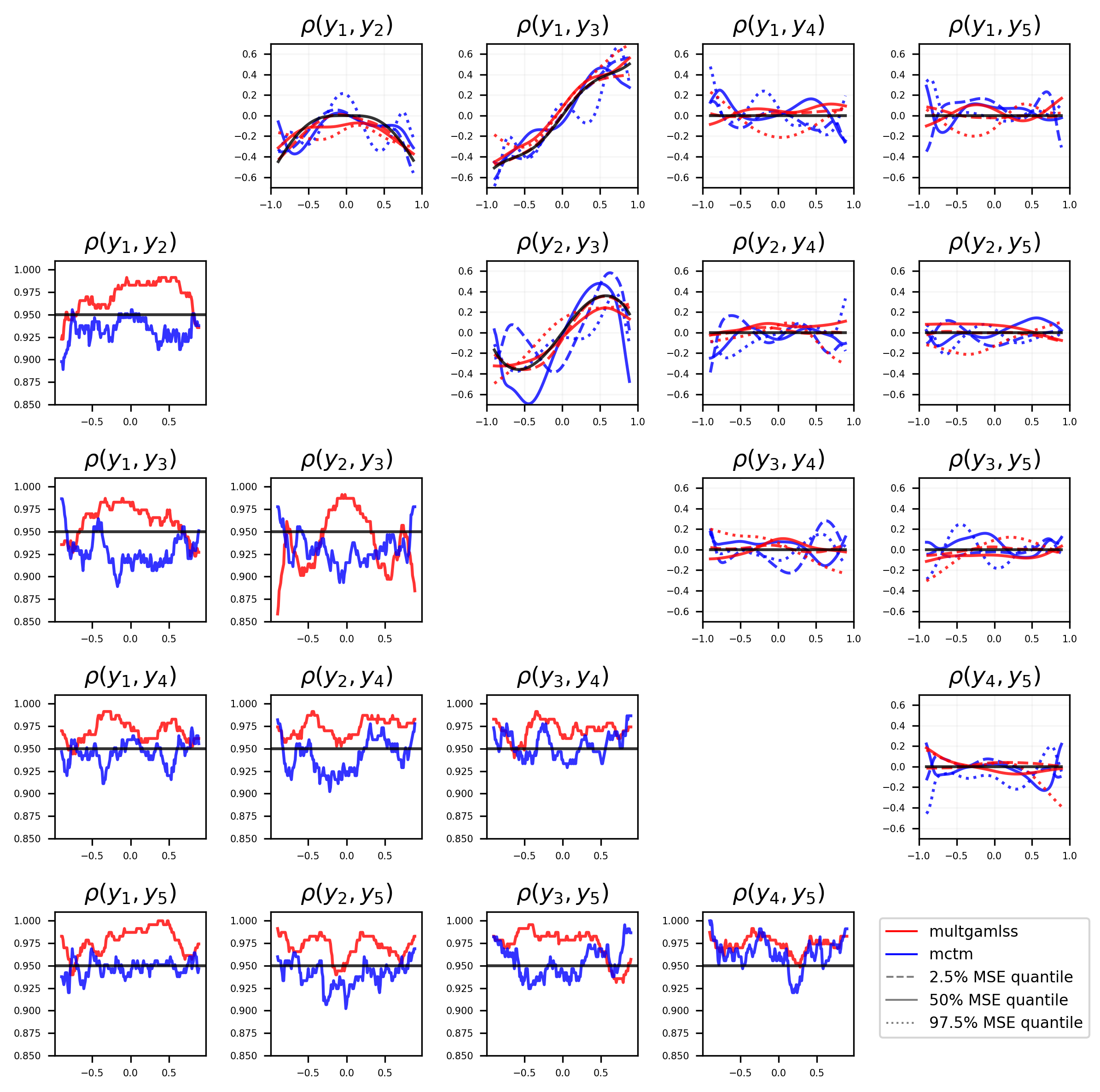
Figure 1: Five dimensional non-Gaussian. $2.5\%$ quantile (dashed), the $50\%$ quantile (bold) and the $95.5\%$ quantile (dotted) quantiles of the MSE-distribution (upper triangle) for multgamlss (red) and mctm (blue) across $250$ repetitions. The black lines correspond to the true effects. Coverage rates for $95\%$ pointwise Bayesian credible set derived through multgamlss (red) and for $95\%$ confidence intervals derived by multgamlss (blue) are shown in the lower triangular plots.

4 Applications

4.1 Childhood Malnutrition in Nigeria

As a first illustration, we consider a data set on childhood malnutrition in Nigeria from 2013 previously analyzed in Klein et al. (2021); Strömer et al. (2023) with data originally taken from the Demographic and Health Survey (DHS, https://dhsprogram.com). While both references use only two of the three available dependent variables (mostly due to model restrictions to bivariate responses), we consider the three variate response vector $(y_{\text{stunting}},y_{\text{wasting}},y_{\text{underweight}})$, where $y_{\text{stunting}}$, $y_{\text{wasting}}$ and $y_{\text{underweight}}$ refer to insufficient height with respect to age, insufficient weight for height, and insufficient weight for age, respectively. Klein et al. (2022) investigate an older data set on malnutrition in India with a three-variate response vector. However, their model incorporates the age of the child cage as the only covariate, even though a large number of demographic and family-related features are available, see Table E.1 in the Online Supplement of Klein et al. (2021).

Model specification

We consider two different models. In the first model, each of the three marginal distributions is assumed to be Gaussian, such that the joint distribution is a multivariate Gaussian distribution with nine predictors $\eta_{k},k=1,\dots,9$ referring to the three marginal means $\mu_{\text{stunting}},\mu_{\text{wasting}}$ and $\mu_{\text{underweight}}$ and logarithms of the standard deviations $\sigma_{\text{stunting}},\sigma_{\text{wasting}}$ and $\sigma_{\text{underweight}}$ as well as the three unrestricted parameters $\lambda_{1},\lambda_{2}$ and $\lambda_{3}$ of the modified Cholesky decomposition of the correlation matrix. In the second model, each of the marginal distributions follows a Student t-distribution. This model incorporates three additional predictors referring to the logarithmic degrees of freedom $\nu_{\text{stunting}},\nu_{\text{wasting}}$ and $\nu_{\text{underweight}}$. In both models each predictor is that used in Strömer et al. (2023) and is modelled additively through four functional effects of cage, the age of the child in months, mage, the mother’s age and body mass index mbmi, her partner’s education edupartner, a discrete spatial effect subregion using the 37 districts in Nigeria and eleven further linear effects of binary and categorical variables, such as munemployed, whether the mother is unemployed and csex, the sex of the child.

Model fits

For the Gaussian model all three margins show clear deviations from normality in the right tail (see Figure B.9 in the Web Appendix). Previous analyses of this data set did not account for these deviations. An inspection of the normalized quantile residuals suggests that the Student t model fits the data slightly better, so that we consider the Student t model for the rest of this analysis.

Estimated effects

The estimated functional and spatial effects coincide well with previous analyzes, see the Web Appendix B for a discussion of the marginal effects.

The correlation structure is strongly influenced by cage. This becomes apparent when we consider the influence of cage on the joint distribution by setting all other covariates to fixed values (mean for continuous variables and mode for binary variables) as illustrated in Figure 2. This figure summarizes univariate marginal densities (diagonal), bivariate margins (lower left) and effects on Spearman’s rho (upper right) for increasing cage. We observe that $y_{\text{stunting}}$ and $y_{\text{wasting}}$ have a negative Spearman’s rho correlation coefficient, which is stronger for children younger than $20$ months. Likewise, $y_{\text{wasting}}$ and $y_{\text{underweight}}$ are positively correlated and the correlation increases within the first 20 months. The rank correlation between $y_{\text{stunting}}$ and $y_{\text{underweight}}$ is overall high without a strong influence of cage. We do not find a strong effect of either edupartner, mage nor mbmi on the correlation structure.

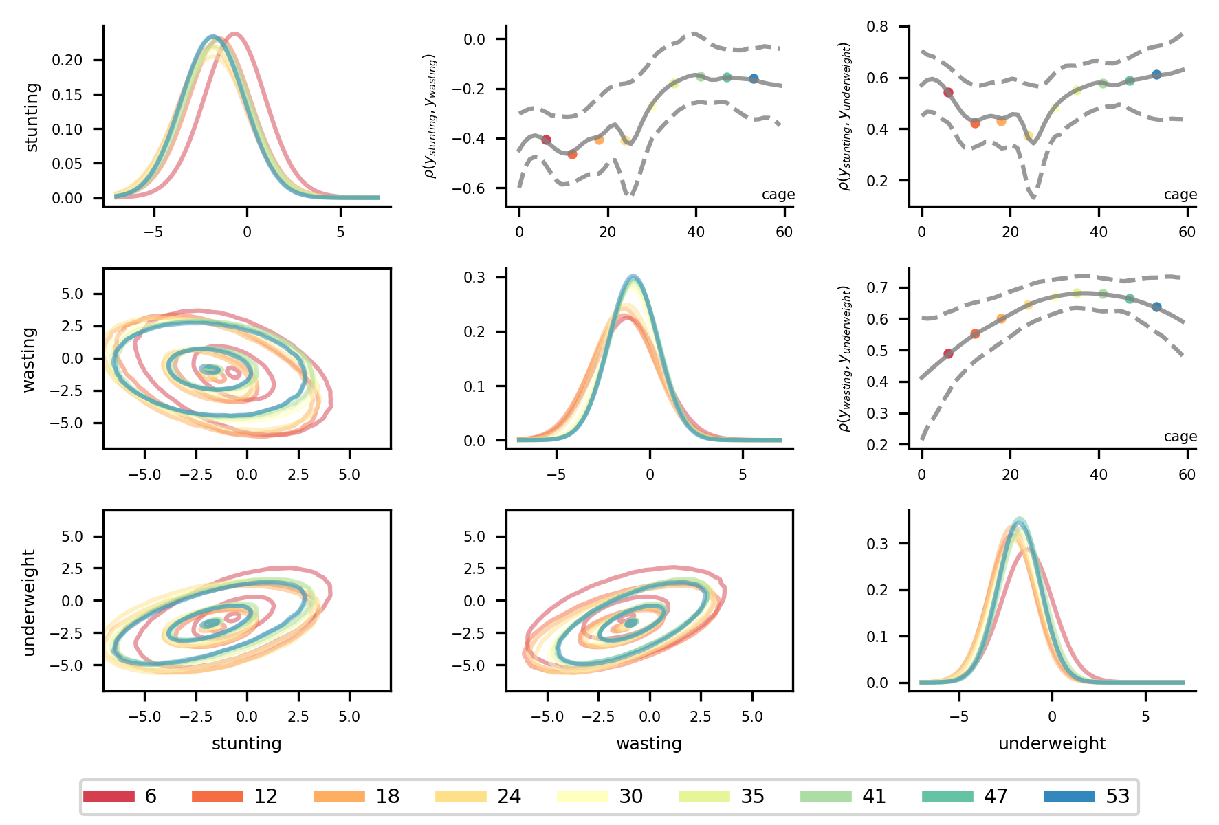
Figure 2: Childhood malnutrition. The effects of cage on a typical child at different ages (indicated by colour). On the main diagonal, the marginal densities are summarized, while bivariate contour plots with levels 0.025, 0.5 and 0.975 are given on the lower triangle. The upper triangle shows the estimated effects on the pairwise Spearmann’s rho correlation coefficient in relation to cage. The posterior mean (bold) and 95% credible intervals (dashed) are given. The dots indicate the different age levels considered.

In Figure 3 we vary subregion while fixing the remaining covariates (mean for continuous variables and mode for binary variables) to investigate the influence of the spatial effect on the joint distribution. The parametric form of the margins allows us to directly consider the influence on $\mathbb{E}\left[y_{j}\right]=\mu_{j}$, the expected values, and $\mathbb{V}\left[y_{j}\right]=\sigma_{j}^{2}\frac{\nu_{j}}{\nu_{j}-2}$, the variances of the univariate marginal distributions, for $j\in\{\text{stunting, wasting, underweight}\}$. The higher values for $\mathbb{E}\left[y_{\text{stunting}}\right]$ and $\mathbb{E}\left[y_{\text{underweight}}\right]$ in regions in southern Nigeria compared to the average indicate a lower risk for stunted growth and insufficient weight for age in these regions. Additionally, the variances $\mathbb{V}\left[y_{\text{stunting}}\right]$ and $\mathbb{V}\left[y_{\text{underweight}}\right]$ are lower in southern regions compared to the north of Nigeria. While Spearman’s rho correlation coefficient $\rho\left(y_{\text{wasting}},y_{\text{underweight}}\right)$ seems to be almost constant with respect to subregion, the spatial effects on $\rho\left(y_{\text{stunting}},y_{\text{wasting}}\right)$ and $\rho\left(y_{\text{stunting}},y_{\text{underweight}}\right)$ are more pronounced and exhibit a similar structure.

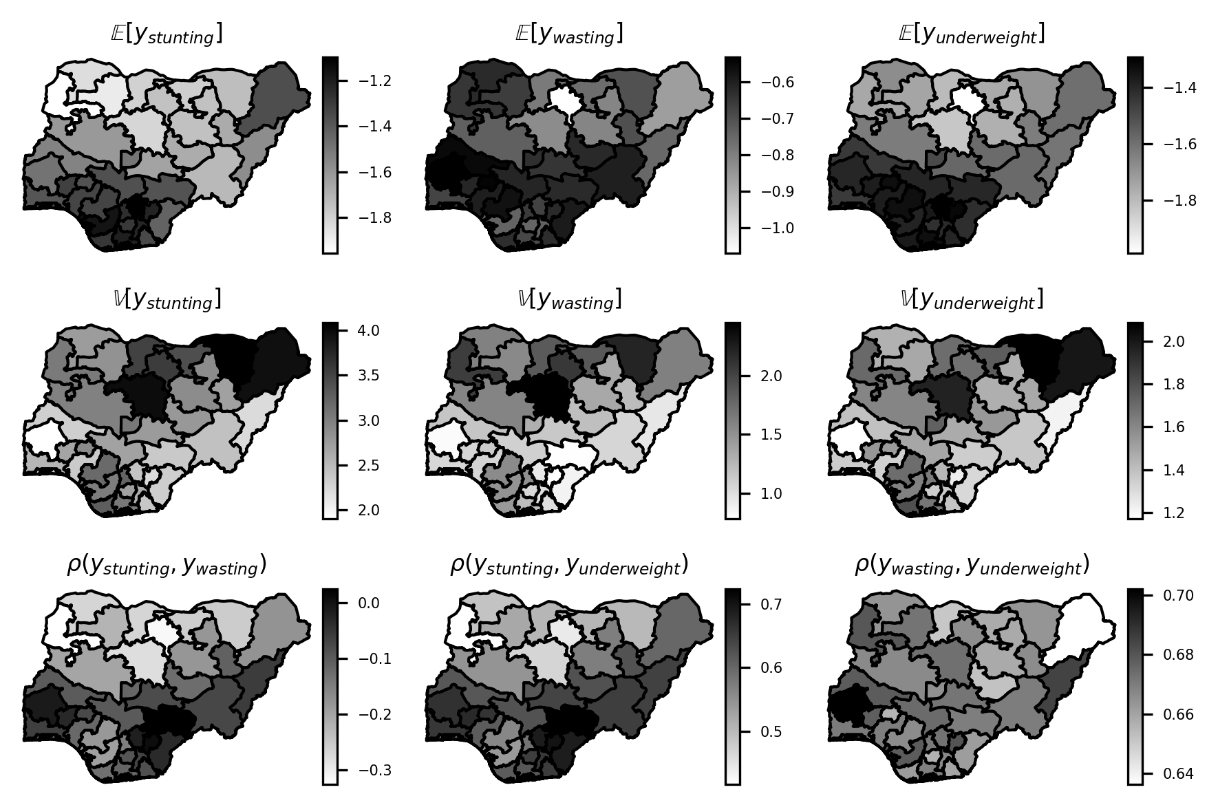
Figure 3: Childhood malnutrition. Spatial effects on a typical child for all $37$ regions. The marginal densities are summarized through the effects on the mean (top row) and the variance (middle row). The bottom row shows estimated effects on the pairwise Spearmann’s rho correlation coefficient in relation to subregion.

4.2 Traffic Detection in Berlin

In the German capital Berlin, several hundred sensors monitor the traffic along main roads. Hourly aggregated data is publicly available through the Senatsverwaltung für Umwelt, Mobilität, Verbraucher- und Klimaschutz and Verkehrsinformationszentrale Berlin (viz.berlin.de). We consider the measures of a single traffic detector located at “Unter den Linden” close to the main building of the Humboldt-Universität zu Berlin (HU) for our analysis. The response variable is four dimensional and consists of the number of cars $y_{c,car}$ and trucks $y_{c,truck}$ passing the sensor, as well as the average speed of the cars $y_{s,car}$ and $y_{s,truck}$ per hour over five years from 2015–2020 leading to a total of $39,739$ data points. Analyzing this four dimensional response $y_{t}=\left(y_{t;c,car},y_{t;s,car},y_{t;c,truck},y_{t;s,truck}\right)^{\top}$ is challenging since it incorporates discrete and continuous components with a complex dependence structure. Descriptive summaries of the data can be found in Figure 4.

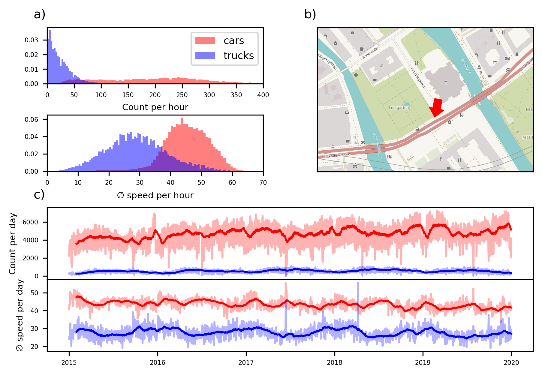
Figure 4: Traffic detection. a) Histograms of the counts per hour (top) and the average speed per hour (bottom) of cars (red) and trucks (blue). b) Position of the traffic detection sensor considered. Map data is taken from open street map. c) Time series representation of the count per day (top) and the average speed per day (bottom). The bold line is a 30-day rolling mean.

Model specification

To gain insights into the temporal traffic dynamics around the HU main building, we model $y_{t}$ jointly through a Gaussian copula with negative binomial distributions for the discrete margins $y_{c,car}$ and $y_{c,truck}$ and Student t distributions for the continuous margins $\log\left(y_{s,car}\right)$ and $\log\left(y_{s,truck}\right)$. Each of the sixteen predictors is

$$\eta^{(\theta)}_{t}=\sum_{h\in\{(c,car),(s,car),(c,truck),(s,truck)\}}\beta^{(\theta)}_{1,h}\widetilde{y_{t;h}}+\beta^{(\theta)}_{2,h}\delta_{t}\widetilde{y_{t;h}},$$

where $\delta_{t}\in\{1,-1\}$ indicates if time point $t$ is on a weekend and $\widetilde{y_{t;h}}$ is the vector of normalized lagged values with lags of $1,2,\ldots,23$ hours, $1,2,\ldots,6$ days, $1,2,3,4,8,12,\ldots,52$ weeks to account for the auto-regressive structure in the data. For our analysis, we consider only time points $t$ for which the full vector of lagged values $\widetilde{y_{t;h}}$ is available.

Model fits

Figure 5 displays normalized quantile residuals for each of the four marginal distributions. The results indicate that the overall fit for the margins is satisfactory. Only, for $y_{(s,truck)}$, there are significant deviations from the distributional assumption in the model, while deviations in the other three marginal distributions are not as pronounced. Minor deviations on the left tail may be attributed to the presence of very small values, which could be due to traffic anomalies, such as line blockage, that are not accounted for in the model. Addressing this issue could involve incorporating additional variables that capture the impact of external factors, such as traffic disruptions or weather conditions. Deviations on the upper tail for $y_{s,car}$ and $y_{s,truck}$ are expected as the Student t margins do not account for the speed of the vehicles being naturally bounded from above. The copula model is preferable over a model with independent margins according to BIC.

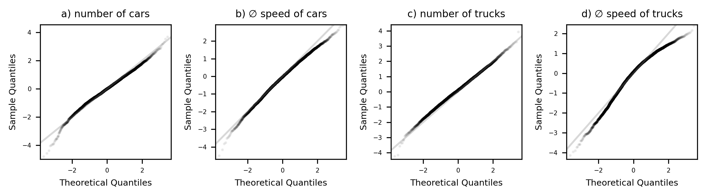
Figure 5: Traffic detection. Normalized qantile residuals for $y_{c,car}$, $\log(y_{s,car})$, $y_{c,truck}$ and $\log(y_{s,truck})$ (from left to right).

Estimated effects

Figure 6 shows the estimated effects $\beta^{(\theta)}_{1,h}-\beta^{(\theta)}_{2,h}$ on the mean parameters of the four marginal distributions, which are the effects for time points on weekdays. We find that the lagged values of the past few hours have the overall strongest effects. Notably, the marginal distributions are not only influenced by lagged values from their respective marginal, but by the full vector $\widetilde{y_{t;h}}$. For example $\mathbb{E}[\log(y_{s,car})]$ is strongly influenced by the number of cars counted in the previous hour. This is reasonable as a high number of cars indicates a busy road resulting in a slower overall speed of vehicles. A description on all fitted effect parameters can be found in Web Appendix B.

The mean and variance of the fitted margins can be calculated for all time points $t$ due to the response distribution being fully parameterized. We find that both marginal count distributions suffer from overdispersion as $\mathbb{V}[y_{t;c,car}]>\mathbb{E}[y_{t;c,car}]$ and $\mathbb{V}[y_{t;c,truck}]>\mathbb{E}[y_{t;c,truck}]$ for all timepoints $t$. The parameter $\omega_{t;3,2}$ controlling the bivariate correlation between $y_{c,truck}$ and $\log\left(y_{s,car}\right)$ is negative for most time points $t$ indicating that a high number of trucks corresponds to the average car driving slower. Similarly, $\omega_{t;4,2}>0$ for most time points $t$ indicating cars and trucks driving faster/slower during similar time periods.

Figure 7 summarizes univariate marginal densities (diagonal) and bivariate margins (lower left) for three different, randomly selected time points showcasing the high flexibility of the fitted model. The bivariate contour plots illustrate the influence of the Gaussian copula and correspond well with our findings described above. For example, we find that $y_{s,car}$ and $y_{s,truck}$ are positively correlated for all three time points.

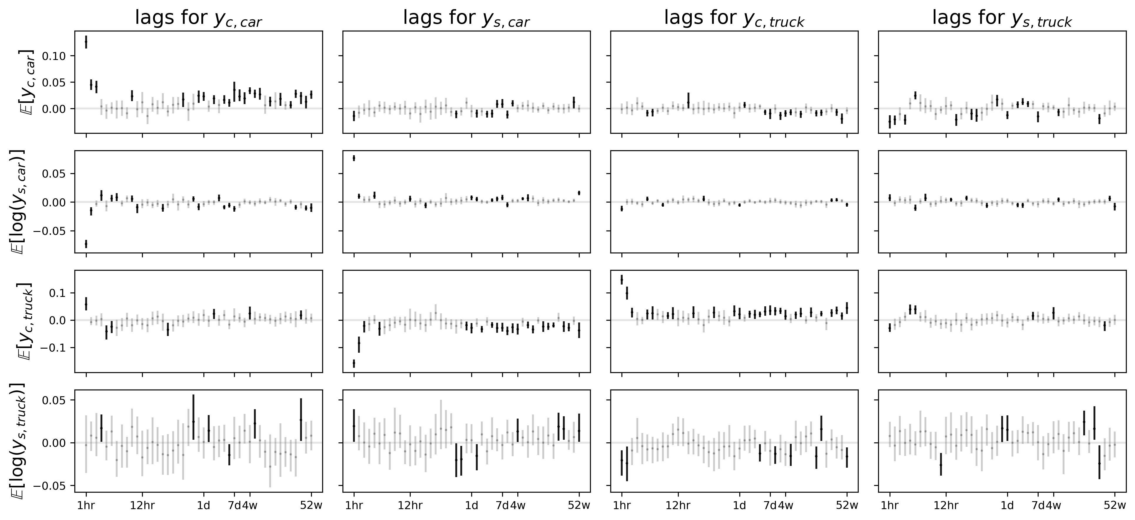
Figure 6: Traffic detection. Posterior mean (dots) and posterior $95\%$ credible intervals (vertical lines) for $\beta^{(\theta)}_{1,h}-\beta^{(\theta)}_{2,h}$, which are the effects for weekdays. If the equally tailed $95\%$ credible interval contains zero, the corresponding effect is grayed. The columns correspond to the standardized lags of $y_{c,car},y_{s,car},y_{c,truck}$ and $y_{s,truck}$ respectively. The rows indicate the mean parameter of the four marginal distributions.

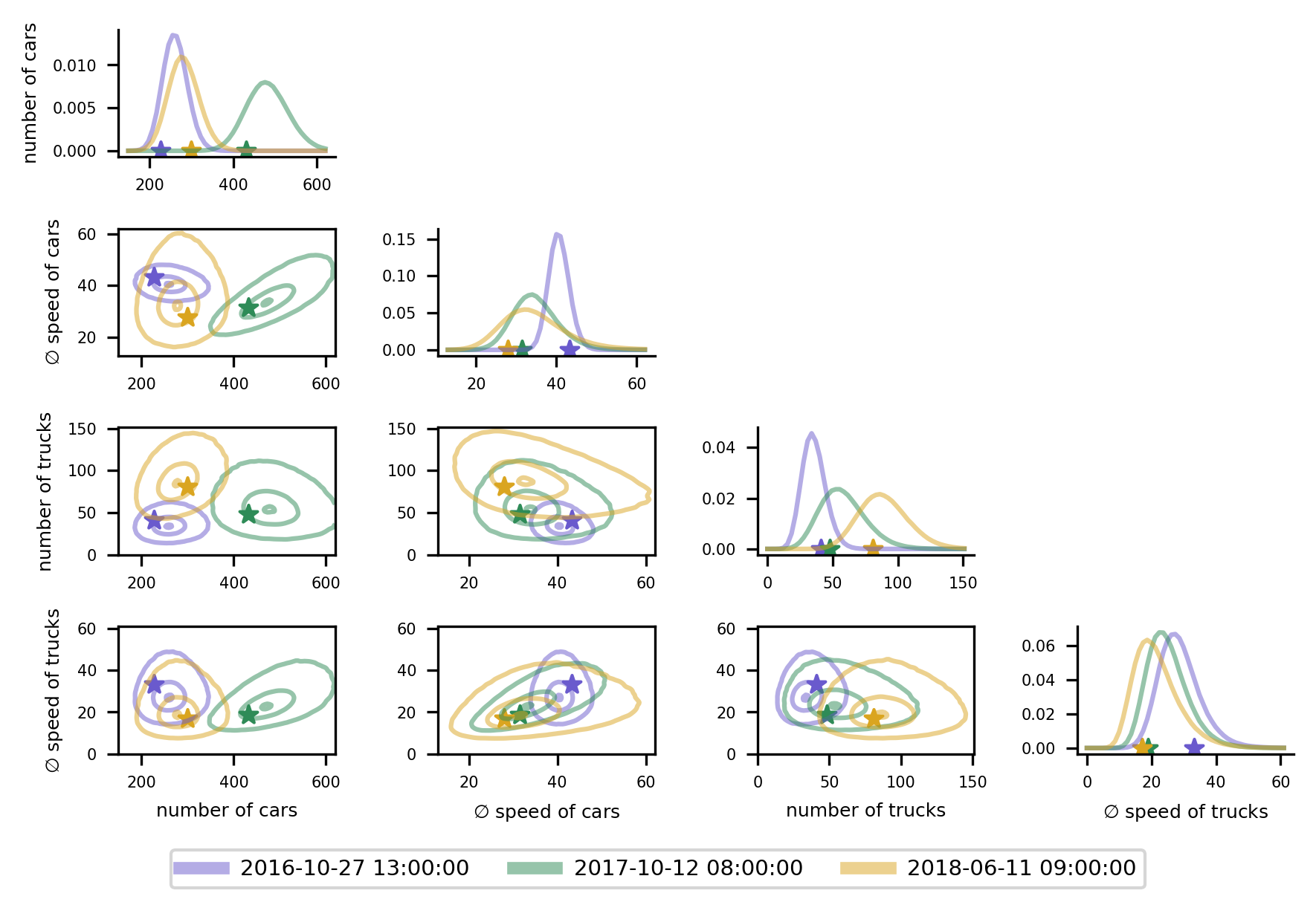
Figure 7: Traffic detection. Univariate marginal densities (diagonal) and bivariate contour plots with levels 0.025, 0.5 and 0.975 (lower triangle) for three different time points (indicated by color). The margins are estimated through a kernel density estimator based on a large sample from the fitted distribution. The observed values at the respective time points are given by stars.

5 Summary and Discussion

This paper introduces a multivariate distributional regression model, which is based on a Gaussian copula to model the dependence structure. The proposed model allows for flexible and independent selection of arbitrary parametric marginal distributions for each response component similar to univariate GAMLSS, while incorporating covariate-dependent additive predictors for each model parameter (including those parameterizing the correlation matrix of the Gaussian copula). Our model complements existing proposals in the field. Our Bayesian treatment has the appeal to allow for uncertainty quantification and interpretability inherited from univariate GAMLSS while not being restricted to bivariate responses as many other existing software packages. In our simulation we find comparable performance in situations where competitors are available yet with increased flexibility and modelling options that we showcase on two real data illustrations.

Although the parametrization of the correlation matrix enables a computationally efficient MCMC sampler, a direct interpretation of additive effects can be challenging. To address this issue, we propose the use of slice plots as a visual inspection tool for the fitted model. However, future research could potentially explore the incorporation of variable and effect selection priors into the model to improve interpretability and simplify model selection.

An additional area for future research would be the exploration of alternative more flexible dependence structures.

References

- (1)
- Browell et al. (2022) Browell, J., Gilbert, C. and Fasiolo, M. (2022). Covariance structures for high-dimensional energy forecasting, Electric Power Systems Research 211: 108446.
- Craiu and Sabeti (2012) Craiu, V. R. and Sabeti, A. (2012). In mixed company: Bayesian inference for bivariate conditional copula models with discrete and continuous outcomes, Journal of Multivariate Analysis 110: 106–120.
- Dunn and Smyth (1996) Dunn, P. K. and Smyth, G. K. (1996). Randomized quantile residuals, Journal of Computational and Graphical Statistics 5(3): 236–244.
- Eilers and Marx (1996) Eilers, P. H. and Marx, B. D. (1996). Flexible smoothing with B-splines and penalties, Statistical Science 11(2): 89–121.
- Fahrmeir et al. (2013) Fahrmeir, L., Kneib, T., Lang, S. and Marx, B. (2013). Regression: Models, Methods and Applications, Springer.
- Fang et al. (2002) Fang, H.-B., Fang, K.-T. and Kotz, S. (2002). The meta-elliptical distributions with given marginals, Journal of Multivariate Analysis 82(1): 1–16.
- Gamerman (1997) Gamerman, D. (1997). Sampling from the posterior distribution in generalized linear mixed models, Statistics and Computing 7: 57–68.
- Gioia et al. (2022) Gioia, V., Fasiolo, M., Browell, J. and Bellio, R. (2022). Additive covariance matrix models: modelling regional electricity net-demand in great Britain, arXiv:2211.07451 .
- Hans et al. (2022) Hans, N., Klein, N., Faschingbauer, F., Schneider, M. and Mayr, A. (2022). Boosting distributional copula regression, Biometrics n/a(n/a).
- Hastie and Tibshirani (1987) Hastie, T. and Tibshirani, R. (1987). Generalized additive models: some applications, Journal of the American Statistical Association 82(398): 371–386.
- Hothorn et al. (2014) Hothorn, T., Kneib, T. and Bühlmann, P. (2014). Conditional transformation models, Journal of the Royal Statistical Society: Series B (Statistical Methodology) 76: 3–27.
- Hult and Lindskog (2002) Hult, H. and Lindskog, F. (2002). Multivariate extremes, aggregation and dependence in elliptical distributions, Advances in Applied Probability 34(3): 587–608.
- Klein et al. (2021) Klein, N., Carlan, M., Kneib, T., Lang, S. and Wagner, H. (2021). Bayesian effect selection in structured additive distributional regression models, Bayesian Analysis 16(2): 545–573.
- Klein et al. (2022) Klein, N., Hothorn, T., Barbanti, L. and Kneib, T. (2022). Multivariate conditional transformation models, Scandinavian Journal of Statistics 49(1): 116–142.
- Klein and Kneib (2016) Klein, N. and Kneib, T. (2016). Simultaneous inference in structured additive conditional copula regression models: a unifying Bayesian approach, Statistics and Computing 26: 841–860.
- Klein, Kneib, Klasen and Lang (2015) Klein, N., Kneib, T., Klasen, S. and Lang, S. (2015). Bayesian structured additive distributional regression for multivariate responses, Journal of the Royal Statistical Society: Series C (Applied Statistics) pp. 569–591.
- Klein, Kneib, Lang and Sohn (2015) Klein, N., Kneib, T., Lang, S. and Sohn, A. (2015). Bayesian structured additive distributional regression with an application to regional income inequality in Germany, Annals of Applied Statistics 9: 1024––1052.
- Krämer et al. (2013) Krämer, N., Brechmann, E. C., Silvestrini, D. and Czado, C. (2013). Total loss estimation using copula-based regression models, Insurance: Mathematics and Economics 53(3): 829–839.
- Lang and Brezger (2004) Lang, S. and Brezger, A. (2004). Bayesian P-splines, Journal of Computational and Graphical Statistics 13(1): 183–212.
- Marra and Radice (2017) Marra, G. and Radice, R. (2017). Bivariate copula additive models for location, scale and shape, Computational Statistics & Data Analysis 112: 99–113.
- Masarotto and Varin (2012) Masarotto, G. and Varin, C. (2012). Gaussian copula marginal regression, Electronic Journal of Statistics 6: 1517–1549.
- Murray et al. (2013) Murray, J. S., Dunson, D. B., Carin, L. and Lucas, J. E. (2013). Bayesian Gaussian copula factor models for mixed data, Journal of the American Statistical Association 108(502): 656–665.
- Muschinski et al. (2022) Muschinski, T., Mayr, G. J., Simon, T., Umlauf, N. and Zeileis, A. (2022). Cholesky-based multivariate Gaussian regression, Econometrics and Statistics .
- Oakes and Ritz (2000) Oakes, D. and Ritz, J. (2000). Regression in a bivariate copula model, Biometrika 87(2): 345–352.
- Paszke et al. (2017) Paszke, A., Gross, S., Chintala, S., Chanan, G., Yang, E., DeVito, Z., Lin, Z., Desmaison, A., Antiga, L. and Lerer, A. (2017). Automatic differentiation in PyTorch, 31st Conference on Neural Information Processing Systems (NIPS2017), Workshop on Autodiff.
- Pitt et al. (2006) Pitt, M., Chan, D. and Kohn, R. (2006). Efficient bayesian inference for gaussian copula regression models, Biometrika 93(3): 537–554.
- Pourahmadi (1999) Pourahmadi, M. (1999). Joint mean-covariance models with applications to longitudinal data: Unconstrained parameterisation, Biometrika 86(3): 677–690.
- Rigby and Stasinopoulos (2005) Rigby, R. A. and Stasinopoulos, D. M. (2005). Generalized additive models for location, scale and shape, Journal of the Royal Statistical Society: Series C (Applied Statistics) 54(3): 507–554.
- Rue and Held (2005) Rue, H. and Held, L. (2005). Gaussian Markov Random Fields: Theory and Applications, Chapman and Hall/CRC.
- Smith and Khaled (2012) Smith, M. S. and Khaled, M. A. (2012). Estimation of copula models with discrete margins via Bayesian data augmentation, Journal of the American Statistical Association 107(497): 290–303.
- Song (2000) Song, P. X.-K. (2000). Multivariate dispersion models generated from Gaussian copula, Scandinavian Journal of Statistics 27(2): 305–320.
- Song et al. (2009) Song, P. X.-K., Li, M. and Yuan, Y. (2009). Joint regression analysis of correlated data using Gaussian copulas, Biometrics 65(1): 60–68.
- Strömer et al. (2023) Strömer, A., Klein, N., Staerk, C., Klinkhammer, H. and Mayr, A. (2023). Boosting multivariate structured additive distributional regression models, Statistics in Medicine 42(11): 1779–1801.
- Sun and Ding (2021) Sun, T. and Ding, Y. (2021). Copula-based semiparametric regression method for bivariate data under general interval censoring, Biostatistics 22(2): 315–330.
- Umlauf et al. (2021) Umlauf, N., Klein, N., Simon, T. and Zeileis, A. (2021). bamlss: A lego toolbox for flexible Bayesian regression (and beyond), Journal of Statistical Software 100(4): 1–53.
- Vatter and Chavez-Demoulin (2015) Vatter, T. and Chavez-Demoulin, V. (2015). Generalized additive models for conditional dependence structures, Journal of Multivariate Analysis 141: 147–167.
- Yee (2010) Yee, T. W. (2010). The VGAM package for categorical data analysis, Journal of Statistical Software 32(10): 1–34.
- Zellner and Huang (1962) Zellner, A. and Huang, D. S. (1962). Further properties of efficient estimators for seemingly unrelated regression equations, International Economic Review 3(3): 300–313.