From elephant to goldfish (and back): memory in stochastic Volterra processes

Abstract.

We propose a new theoretical framework that exploits convolution kernels to transform a Volterra path-dependent (non-Markovian) stochastic process into a standard (Markovian) diffusion process. This transformation is achieved by embedding a Markovian "memory process" (the goldfish) within the dynamics of the non-Markovian process (the elephant). Most notably, it is also possible to go back, i.e., the transformation is reversible. We discuss existence and path-wise regularity of solutions for the stochastic Volterra equations introduced and we propose a numerical scheme for simulating the processes which exhibits a remarkable convergence rate of $1/2$. In particular, in the fractional kernel case, the strong convergence rate is independent of the roughness parameter, which is a positive novelty in contrast with what happens in the available Euler schemes in the literature in rough volatility models.

Keywords: Stochastic Volterra Equations, Markov process, Fractional Integrals, Euler Scheme, Rough Volatility

MSC 2020 Classification: 60G22, 65C20, 91G20, 91G60, 91G80

1. Introduction

Over the past few years, there has been a contentious discussion surrounding the inclusion of memory in the volatility process. This debate has taken place not only within academic circles but also within the banking industry. Central to this dispute is the fundamental question of whether it is appropriate to model volatility using a non-Markovian stochastic process. The mathematical finance community has therefore split into two main streams, based on two types of paradigm. The first category, to address the limitations of Markovian models and to account for volatility persistence, has introduced a new family of models where the volatility process is driven by a fractional Brownian motion (fBM), which is a non-Markovian process. The empirical evidence of persistence initially inspired the introduction of the fractional stochastic volatility (FSV) model in [9]. This model is based on a fractional Ornstein-Uhlenbeck process driven by a fBM with a Hurst parameter $H$ greater than $1/2$. It provides a continuous-time stochastic volatility model with long memory properties. More recently, researchers have shifted towards using a fBM with $H$ less than $1/2$ to account for roughness in volatility trajectories, see [3, 14]. In this case volatility paths exhibit more irregularity compared to those generated by the traditional Brownian motion ($H=1/2$). These models, known as rough volatility models, have gained significant popularity in the academic literature. Their success lies in their ability to capture the main stylized facts of historical volatility time series and effectively fit option smiles observed in the SPX market, still keeping a parsimonious parameter structure.
The second paradigm is rooted in the belief that financial markets exhibit a discernible pattern of path-dependent volatility [18, 11]. In this approach, the volatility is assumed to be a function of past returns involving an exponential kernel as a decay factor, see e.g. [19, 20, 6] and references therein. Notably, there is no requirement to introduce a fractional Brownian motion in this methodology. Path-dependent volatility models (PDV) do not require additional sources of randomness to generate rich spot-vol dynamics, as they explain volatility in a purely endogenous manner. Consequently, prices derived from these models are unique under the risk-neutral measure.
Despite the limitations in analytical tractability, rough volatility models have taught us that incorporating memory into processes, even at the expense of losing the Markovian structure and semi-martingale property, is highly valuable for replicating most stylized market effects. From a mathematical perspective, the presence of a kernel involving memory in the stochastic integral opens the door to the theory of stochastic Volterra processes in the modeling of volatility.

Even if the contributions in the literature to deal with the non-Markovian structure in rough volatility models are present, there is still a challenge when dealing with numerical schemes for pricing and calibration purposes, which typically turn out to be extremely time consuming because the strong (and weak) rate of convergence deteriorates as $H$ goes to zero e.g. [7, 12, 22]. Any attempt to transform the problem into one that is easier to solve is obviously crucial. The key point is to accurately incorporate a dependence on the past in the volatility dynamics, rather than solely focusing on the fractional Brownian motion itself.

Our paper fits into this perspective: we propose a new theoretical framework where we exploit the possibility to transform, via a convolution kernel, a Volterra path-dependent (non-Markovian) stochastic process into a standard (Markovian) diffusion process without memory. What is more, we provide a way to go back and forth (this explains the title of the paper). More precisely, we embed, using kernels associated with different decay laws (including but not limiting ourselves to power laws, corresponding to rough models), what we call the Markovian volatility memory process $\xi$, in the dynamics of the relevant non-Markovian process $X$.

The new framework requires a careful investigation in terms of existence and path-wise regularity of the solutions of the stochastic Volterra equations therein introduced. This is performed in the first part of the paper, where we also illustrate the methodology that allows one to transform the Volterra process into a Markovian diffusion process and back. Then, we propose a numerical scheme for the simulation of this couple of processes, together with a thorough analysis of its numerical error and convergence rate. In this context, we prove a remarkable result: the strong rate of convergence of the numerical scheme is $1/2$ and, in the case when the kernel is fractional, it is independent of the parameter $H$, characterizing the roughness of the paths of the Volterra process. This is a bold improvement when compared with the performance of the Euler schemes for the solution of Volterra SDEs arising from rough volatility models, whose strong rate of convergence is $H$ (with $H$ being often set to be close to $0.1$, for financial applications), see e.g. [23, 34]. An additional noteworthy by-product of our methodology is its flexibility, as it allows Volterra processes to be transformed into processes that do not necessarily possess Markovian characteristics. The determinative factor lies in the definition of the (pseudo-)inverse of the kernel employed in the transformation. While it is preferable, particularly for practical applications, to define the pseudo-inverse so that the transformed process becomes Markovian, as exemplified in the paper, this choice is specific to the situation at hand. The main point is to be able to exploit the structure of the transformed process.

Our approach can be seen as a generalization of the fractional Heston model introduced in [17] (and further discussed in [2]), via the use of a more general family of kernels together with the introduction of a non-deterministic initial condition depending on time. The contribution of this quantity is not just in terms of adding some technicalities in the proofs, but it can be seen as a burst of memory at $t=0$, needed to restore the memory of the process of what was somehow happening before the initial time. Another attempt of generalizing [17] can be found in [22]. Our approach is somehow reminiscent of theirs but the purpose, as well as the tools exploited therein, differ from ours. In particular, our theoretical study and the simulation scheme we propose are completely different. Furthermore, as a consequence of our formalization, we get for free a path-dependent Volterra equation, that surprisingly turns out to be easily numerically solvable. Last but not least, we get strong existence and uniqueness of solutions for the equation of the memory process, $\xi$, and, by fractional integration of it, of the process $X$ itself. Our work is also related to [21], who independently investigated a similar stochastic Volterra integral equation with power kernel and proved the existence, uniqueness and Markov property for the lifted stochastic evolution equation defined on an (infinite dimensional) Hilbert space. We emphasize that the performance of our numerical results is due to the fact we are able to work in finite dimension.

The rest of the paper is organized as follows. In Section 2, we develop a preliminary yet detailed investigation of the properties of the Volterra-type processes of interest for us. In particular, after establishing the notation used in the reminder of the paper, we define the convolution transform as well as the concept of $\rho$-pseudo-inverse co-kernel. Finally, we present some preliminary existence and regularity results to guarantee the well-posedness of the processes we introduce. Then, in Section 3 we prove and comment the two-way connection between our path-dependent Volterra Equation and an associated standard SDE. We first present an informal argument and then the detailed proof is discussed in Section B.2. Therein a thorough analysis of the mathematical features of the approach is developed, proving in particular strong existence and uniqueness of solutions and the Hölder regularity of sample paths for our processes. In Section 4 we study the continuous time Euler scheme and their convergence for both the elephant and the goldfish processes. In Section 5 we deal with the fractional kernel case, in the case of interest for the financial literature, i.e., when the Hurst index $H\in(0,\frac{1}{2})$. We adapt the theorem obtained in the previous sections to this setting: we first provide well-posedness results and path-wise regularity results and we then study the Euler scheme and its convergence. The main result concerns the strong rate of convergence. This is proved to be $1/2$, independently of $H$. Finally, in Section 5.3 we provide some simulations.

We gather in Appendix A some material on fractional calculus and Laplace transforms for the reader’s convenience and in Appendix B the technical proofs. Appendix B contains most of the proofs of Lemmas, Propositions and Theorems. Appendix C concludes the paper with a deep insight into simulating the Euler scheme for the elephant process.

2. Mathematical preliminaries and prerequisites

2.1. Notation

Let us consider a fixed finite time horizon $T>0$ and a complete filtered probability space $(\Omega,\mathcal{F},\mathbb{P};\mathbb{F})$, with $\mathbb{F}=(\mathcal{F}_{t})_{t\in[0,T]}$. On this probability space we consider an $\mathbb{R}$-valued random variable $X$ and an $\mathbb{R}$-valued random process, $Y=(Y_{t})_{t\in[0,T]}$. We denote by $\textrm{AC}([0,T])$ the space of absolutely continuous functions on $[0,T]$. For $x\in\mathbb{R}$, we denote by $\delta_{x}$ the Dirac delta distribution centred at $x$. Given a function $f:(t,x)\in[0,T]\times\mathbb{R}\rightarrow\mathbb{R}$ which is Lipschitz in $x$, uniformly in time, $t$, we denote by $[f]_{{\rm Lip},x}$ its Lipschitz constant. The set of functions $f:\mathbb{R}_{+}\to\mathbb{R}_{+}$ such that $\int_{0}^{T}|f(t)|^{p}dt<+\infty$, for every $T>0$, is denoted by ${L}^{p}_{loc}(\mathbb{R}_{+},{\rm Leb}_{1})$, $1\leq p<\infty$. In case of no ambiguity, we use the notation ${L}^{p}_{loc}(\mathbb{R}_{+})$ or simply ${L}^{p}_{loc}$. For $1\leq p<\infty$, we denote by $\|X\|_{p}$ the $p$-norm of $X$, i.e. $\|X\|_{p}:=\mathbb{E}[|X|^{p}]^{\frac{1}{p}}$, and by $\|Y\|_{\mathcal{L}^{p}}$ the $\mathcal{L}^{p}$-norm of the stochastic process $Y$, i.e. $\|Y\|_{\mathcal{L}^{p}}:=\mathbb{E}\left[\int_{0}^{T}|Y_{s}|^{p}ds\right]^{\frac{1}{p}}$. For $p>0$ we denote by $L^{p}(\mathbb{P})$ the set of real-valued random variables $X$ such that $\mathbb{E}[|X|^{p}]<\infty$. Finally, $\mathcal{L}^{2}:=\mathcal{L}^{2}([0,T])$ represents the set of real-valued stochastic processes $Y=(Y_{t})_{t\in[0,T]}$ which are $\mathbb{F}-$progressively measurable and such that $\|Y\|_{\mathcal{L}^{2}}^{2}<+\infty$.

Let us stress that the stochastic basis $(\Omega,\mathcal{F},\mathbb{P};\mathbb{F})$, with $\mathbb{F}={(\mathcal{F}_{t})}_{t\in[0,T]}$ is assumed to be rich enough to model all the randomness in our model and such that a standard Brownian motion $\{W_{t},t\in[0,T]\}$ is defined on it.

2.2. Convolution transforms

In order to introduce our convolution transform, first we have to recall the notion of convolution kernel.

Definition 2.1.

A convolution kernel is a function $K:\mathbb{R}_{+}\to\mathbb{R}_{+}$ such that, for $0\leq s\leq t\leq T$, $K(t,s)=K(t-s,0)=K(t-s)$ and $\int_{0}^{T}K(t)dt>0$, for every $T>0$.

Given a convolution kernel, $K$, and a function, $f$, on $\mathbb{R}_{+}$, their convolution $(K\star f)$ is defined as

$$(K\star f)(t):=\int_{0}^{t}K(t-s)f(s)ds,$$ (2.1)

for all $t<T$ such that the above integral exists finite. A complete list of properties of $(K\star f)$ can be found in [16, Chapter 2, Section 2.2]. In particular, in [16, Theorem II.2.2 and Corollary II.2.3] the authors prove that, for $K\in L^{1}_{\textrm{loc}}(\mathbb{R}_{+})$ and $f\in L^{p}_{\textrm{loc}}(\mathbb{R}_{+})$, for some $p\in[1,\infty]$, the convolution $(K\star f)\in L^{p}_{\textrm{loc}}(\mathbb{R}_{+})$. Now, with a slightly different notation, we introduce a stochastic version of the Lebesgue integral in Equation (2.1). Given a square-integrable stochastic process $Y\in\mathcal{L}^{2}$, we define the family of random variables:

$${(K\star Y)}_{t}:=\int_{0}^{t}K(t-s)Y_{s}ds,\quad 0\leq t\leq T,$$ (2.2)

such that the above integral exists finite $\mathbb{P}$-a.s. Moreover, we introduce the following stochastic Itô integral of convolution type:

$${(K\stackrel{{\scriptstyle W}}{{\star}}Y)}_{t}:=\int_{0}^{t}K(t-s)Y_{s}dW_{s},\quad 0\leq s\leq t\leq T,$$ (2.3)

such that the above integral is well defined (e.g., when the integrand is in $\mathcal{L}^{2}$). In Table 1 we list the most relevant kernels that appear in the literature. In particular, the Gamma kernel is denoted here by $K_{c,\alpha,\rho}$, for positive $c,\alpha,\rho$.

	$K(t)$	Notation	Domain
Constant	$c$	$K_{c,1,0}$	$c>0$
Fractional	$c\frac{t^{\alpha-1}}{\Gamma(\alpha)}$	$K_{c,\alpha,0}$	$c>0,\alpha>0$
Exponential	$ce^{-\rho t}$	$K_{c,1,\rho}$	$c>0,\rho>0$
Gamma	$ce^{-\rho t}\frac{t^{\alpha-1}}{\Gamma(\alpha)}$	$K_{c,\alpha,\rho}$	$c>0,\alpha>0,\rho>0$

Table 1. Some examples of kernels.

2.3. First existence and path-regularity results

Before introducing our new class of stochastic Volterra equations, we prove existence and path-regularity for the stochastic process $X$ defined as

$$X_{t}=\xi^{0}+\int_{0}^{t}K(t-s)Y_{s}dW_{s},\quad t\in[0,T],$$ (2.4)

where $K$ is a convolution kernel, the process $Y\in\mathcal{L}^{2}$, $W$ is the Brownian motion defined on our filtered probability space $(\Omega,\mathcal{F},\mathbb{P};\mathbb{F})$ and $\xi^{0}$ is a random variable defined on the same probability space and assumed to be independent of $W$. So, $\xi^{0}\in\mathcal{F}_{0}$ and, when useful, we use the notation $\mathbb{F}=\mathbb{F}^{\xi^{0},W}$. For simplicity, as it is standard in the literature on SDEs with random initial condition (see [27, Theorem 2.9]), we assume that $\xi^{0}\in L^{p}(\mathbb{P})$ with $p\geq 2$. Let us notice that a more general existence and uniqueness result for stochastic Volterra equations is given in [24, Thm 1.1] for $\xi^{0}\in L^{0}(\mathbb{P})$. In the context of the class of stochastic Volterra equations of interest to us, this Theorem represents an improvement with respect to [36, Thm. 3.1], which is stated for stochastic Volterra equations in Banach spaces with $\xi^{0}\in L^{\infty}(\mathbb{P})$. Nevertheless, for the reader’s ease we detail its proof in Appendix B.1.

Lemma 2.2.

Let $\xi^{0}\in L^{p}(\mathbb{P})$, with $p\geq 2$, and assume that the following two conditions are satisfied:

• $\sup_{t\in[0,T]}||Y_{t}||_{2}<+\infty$;

• there exists $\beta>1$ such that $\int_{0}^{T}K(t)^{2\beta}dt<+\infty$, for all $T>0$.

Then, there exists a unique ${(\mathcal{F}_{t})}_{t\in[0,T]}$-adapted process $X$ such that, for almost all $t\geq 0$,

$$X_{t}=\xi^{0}+\int_{0}^{t}K(t-s)Y_{s}dW_{s},\quad\mathbb{P}\textrm{-a.s.}$$

Moreover, if there exist $\theta\in(0,1)$ and $p>\frac{1}{\theta\wedge\frac{\beta-1}{2\beta}}$, such that:

• $\sup_{t\in[0,T]}\|Y_{t}\|_{p}<+\infty$;

• for some $C_{K}>0$ and $\delta\in(0,T)$,

  $$\left(\int_{0}^{T}\left[K((\delta+v)\wedge T)-K(v)\right]^{2\beta}dv\right)^{\frac{1}{2\beta}}\leq C_{K}\delta^{\theta};$$

then the stochastic process $X$ has a path-wise continuous modification whose trajectories are locally $a$-Hölder continuous for any $a\!\in\left(0,(\theta\wedge\frac{\beta-1}{2\beta})-\frac{1}{p}\right)$.

3. From path-dependent Volterra to standard SDEs

The aim of this section is to investigate a class of path-dependent Volterra SDEs that is associated to a convolution kernel $K$ when it admits what we call a $\rho$-pseudo-inverse co-kernel $\widetilde{K}$. As stated in the introduction they are particularly relevant because of the direct link with a standard SDE that can be associated to them in a very natural way. Therefore, in this section not only we present such a class of Volterra SDEs but we also detail the two-fold connection between the non-Markovian process and Markovian one.

3.1. The $\rho$-pseudo-inverse co-kernel

Let us start by providing the definition of $\rho$-pseudo-inverse co-kernel, the key ingredient in the formal definition of class of Volterra SDEs we are interested in.

Definition 3.1.

A $\rho$-pseudo-inverse co-kernel with respect to $K:=K_{\cdot,\cdot,\rho}$, with $\rho\geq 0$, is a continuous kernel $\widetilde{K}:\mathbb{R}_{+}\to\mathbb{R}_{+}$ satisfying, for every $t\geq 0$,

$$(K\star\widetilde{K})(t)=(\widetilde{K}\star K)(t)=e^{-\rho t}.$$ (3.1)

For some examples of kernels and the corresponding co-kernels see Table 2.

Remark 3.2.

We recall here the definition of one dimensional functional resolvent of the first kind, which can be found e.g. in [16, Def. 5.5.1] (see also [2]). Given $K\in{L}^{1}_{loc}(\mathbb{R}_{+})$, a function $r$ belonging to ${L}^{1}_{loc}(\mathbb{R}_{+})$ is called functional resolvent of the first kind of $K$ if

$$(K\star r)(t)=(r\star K)(t)=1,$$

for all $t\in\mathbb{R}_{+}$. So, when $\rho$ is equal to zero, $\widetilde{K}$ is the functional resolvent of the first kind of $K$.
For $\rho\neq 0$, we find that $\widetilde{K}$ in Definition 3.1 is $\widetilde{K}(u)=e^{-\rho u}\overline{r}(u)$, where $\overline{r}$ is the functional resolvent of the first kind of $\overline{K}(u):=e^{\rho u}K(u)$. Indeed, $\overline{r}$ by definition satisfies

$$\int_{0}^{t}\overline{K}(t-s)\overline{r}(s)ds=\int_{0}^{t}K(t-s)e^{\rho(t-s)}\overline{r}(s)ds=1,$$

which is equivalent to $\int_{0}^{t}K(t-s)\widetilde{K}(s)ds=e^{-\rho t},$ as $\widetilde{K}(s):=e^{-\rho s}\overline{r}(s)$.

As we are going to make an extensive use of kernels and co-kernels, there are a few properties of these mathematical tools that is worth to highlight at this point.

First of all, by applying Fubini-Tonelli’s Theorem we find

$$\int_{0}^{2T}e^{-\rho u}du =\int_{0}^{2T}(\widetilde{K}\star K)(u)du=\int_{0}^{2T}\left(\int_{0}^{u}K(u-s)\widetilde{K}(s)ds\right)du$$

$$=\int_{0}^{2T}\widetilde{K}(s)\int_{0}^{2T-s}K(v)dvds\geq\int_{0}^{T}\widetilde{K}(s)ds\int_{0}^{T}K(v)dv,$$

so that if (the restriction to $[0,T]$ of) $K\!\in L^{1}([0,T],{\rm Leb}_{1})$ and $K$ is a convolution kernel (recall Definition 2.1), then, for every $T>0$, $\int_{0}^{T}\widetilde{K}(s)ds<\infty$.

In the second place, exploiting the positivity of $K$, we obtain that $\widetilde{K}$ is a convolution kernel, too, as it also satisfies $\int_{0}^{T}\widetilde{K}(s)ds>0$.

Finally, for notational homogeneity, we often denote $\int_{0}^{t}\widetilde{K}(s)ds$ as the convolution product:

$$\int_{0}^{t}\widetilde{K}(s)ds=(\mbox{\bf 1}\star\widetilde{K})(t)=(\widetilde{K}\star\mbox{\bf 1})(t)=:\widetilde{\varphi}(t).$$ (3.2)

Being $\widetilde{K}$ continuous on $(0,+\infty)$ and non-negative, $\widetilde{\varphi}(t)=(\widetilde{K}\star\mbox{\bf 1})(t)$ is differentiable and non-decreasing. Moreover, if $\widetilde{K}$ is non-increasing, $\widetilde{\varphi}$ is concave.

	$K$	$K(t)$	$\widetilde{K}$	$\widetilde{K}(t)$
Constant	$K_{c,1,0}$	$c$	$\frac{\delta_{0}}{c}$	$\frac{\delta_{0}(t)}{c}$
Fractional	$K_{c,\alpha,0}$	$c\frac{t^{\alpha-1}}{\Gamma(\alpha)}$	$K_{\frac{1}{c},1-\alpha,0}$	$\frac{1}{c}\frac{t^{-\alpha}}{\Gamma(1-\alpha)}$
Exponential	$K_{c,1,\rho}$	$ce^{-\rho t}$	$\frac{1}{K_{c,1,\rho}}\delta_{0}$	$c^{-1}e^{\rho t}\delta_{0}(t)$
Gamma	$K_{c,\alpha,\rho}$	$ce^{-\rho t}\frac{t^{\alpha-1}}{\Gamma(\alpha)}$	$K_{\frac{1}{c},1-\alpha,\rho}$	$\frac{1}{c}e^{-\rho t}\frac{t^{-\alpha}}{\Gamma(1-\alpha)}$

Table 2. Examples of co-kernels.

3.2. From elephant to goldfish (and back).

We are finally ready to introduce the family of processes we are interested in. We always work under the following assumption.

Assumption 3.3 (Stochastic Fubini).

We assume interchangeability of Lebesgue and stochastic integration.

Sufficient conditions for interchanging the order of ordinary integration (with respect to a finite measure) and stochastic integration (with respect to a square integrable martingale) are given in [25, Thm. 1], see also [32, Thm. IV.65].

The class of Volterra SDEs we focus on formally reads, for $t\in[0,T]$,

$$X_{t}=\xi^{0}+\int_{0}^{t}K(t-s)b\left(s,(\widetilde{K}\star X)_{s}\right)ds+\int_{0}^{t}K(t-s)\sigma\left(s,(\widetilde{K}\star X)_{s}\right)dW_{s},$$

where $\xi^{0}$ is a random variable assumed to be independent of $W$ and $b,\,\sigma:[0,T]\times\mathbb{R}\rightarrow\mathbb{R}$ are Borel measurable functions. The key feature of the non-Markov stochastic process $X$ above is the nested dependency in the coefficients appearing in the SDEs. Indeed, the transformation from non-Markov to Markov, and back, is achieved by embedding a Markovian "memory process" (the goldfish, which will be denoted by $\xi$) within the dynamics of the non-Markovian process $X$ (the elephant).

The following theorem, whose proof is postponed to Appendix B.2, emphasizes the connection between the class of path-dependent Volterra SDEs, represented by the process $X$ above, whose solutions are the elephant (processes), and standard Brownian SDEs, represented by the process $\xi$ which we will introduce in a few lines, whose solutions are the goldfish (processes). Moreover, it provides existence and uniqueness results.

Theorem 3.4.

Let $\rho\geq 0$ and consider Equation (3.3), namely

$$X_{t}=\xi^{0}+\int_{0}^{t}K(t-s)b\left(s,(\widetilde{K}\star X)_{s}\right)ds+\int_{0}^{t}K(t-s)\sigma\left(s,(\widetilde{K}\star X)_{s}\right)dW_{s},$$ (3.3)

where the kernels $K$ and $\widetilde{K}$ satisfy the condition in Equation (3.1). If there exist $\beta>1$ and $\theta\!\in(0,1)$, such that:

• the kernel $K$ satisfies, for some $C_{K}>0$ and $\delta\in(0,T)$:

  $$\int_{0}^{T}K(t)^{2\beta}dt<+\infty\quad\mbox{ and }\quad\left(\int_{0}^{T}\left[K((\delta+v)\wedge T)-K(v)\right]^{2\beta}dv\right)^{\frac{1}{2\beta}}\leq C_{K}\delta^{\theta};$$

• the Borel functions $b$ and $\sigma$ defined on $[0,T]\times\mathbb{R}$ are Lipschitz in $x$ uniformly in $t\!\in[0,T]$, and uniformly bounded at $x=0$:

  $$(i)\;\text{for all }\,t\!\in[0,T],\;\text{for all }\,x,\,y\!\in\mathbb{R},$$

  $$\qquad\qquad|b(t,x)-b(t,y)|\leq[b]_{{\rm Lip},x}|x-y|\quad\mbox{and}\quad|\sigma(t,x)-\sigma(t,y)|\leq[\sigma]_{{\rm Lip},x}|x-y|$$ (3.4)

  $$(ii)\;\sup_{t\in[0,T]}|b(t,0)|+|\sigma(t,0)|<+\infty;$$ (3.5)

• $\xi^{0}\!\in L^{0}(\mathbb{P})$, i.e., it is $\mathbb{P}$-$a.s.$ finite,

then Equation (3.3) has a pathwise continuous strong solution $(X_{t})_{t\in[0,T]}$ of the form:

$$X_{t}=e^{-\rho t}\frac{d}{dt}\left[\big{(}(e^{\rho\cdot}K)\star\xi\big{)}_{t}\right],\quad t\!\in[0,T],$$

where $\xi=(\xi_{t})_{t\in[0,T]}$ is the unique (pathwise continuous) strong solution to the diffusion SDE

$$\xi_{t}=\xi^{0}\,e^{\rho t}(\mbox{\bf 1}\star\widetilde{K})(t)+\int_{0}^{t}\widetilde{b}(s,\xi_{s})ds+\int_{0}^{t}\widetilde{\sigma}(s,\xi_{s})dW_{s},\quad\xi_{0}=0,$$ (3.6)

with coefficients

$$\widetilde{b}(u,x) =e^{\rho u}b(u,e^{-\rho u}x)\quad\mbox{ and }\quad\widetilde{\sigma}(u,x)=e^{\rho u}\sigma(u,e^{-\rho u}x).$$ (3.7)

Theorem 3.4 provides a new stochastic working framework, which makes a solid and clear connection between the Markovian and the non-Markovian worlds. Moreover, it represents a real theoretical bridge, since it is possible to move both forward and backward. A peculiar feature of Equation (3.6) is the deterministic term $\xi^{0}\,e^{\rho t}(\widetilde{K}\star\mbox{\bf 1})(t)$, which vanishes only at time $t=0$ (implying that the starting value for the process $\xi$ is $\xi_{0}=0$), while, immediately after time $t=0$, it has an instantaneous effect on the trajectories of $\xi$, which bump up. It may be seen as a way of including in the process some memory of its the past history (the one before $t=0$), since the very beginning. A visual effect of this can be seen in the simulations in Section 5.3.3.

3.3. An informal intuition

Since the proof of Theorem 3.4 is postponed to Appendix B.2, we provide here an informal argument to provide some intuition without going into the details and technicalities of the proper proof. Let us start by noticing that the Volterra path-dependent SDE in Equation (3.3) may be rewritten in terms of convolution as

$$X=\xi^{0}+K\star b(\cdot,(\widetilde{K}\star X)_{\cdot})+K\stackrel{{\scriptstyle W}}{{\star}}\sigma(\cdot,(\widetilde{K}\star X)_{\cdot}).$$

As a consequence, when working under Assumption 3.3, convoluting $X$ with $\widetilde{K}$, using the associativity of the convolution operators together with the identity in Equation (3.1), we find

$$\widetilde{K}\star X =\xi^{0}\,(\widetilde{K}\star\mbox{\bf 1})+(\widetilde{K}\star K)\star b(\cdot,(\widetilde{K}\star X)_{\cdot})+(\widetilde{K}\star K)\stackrel{{\scriptstyle W}}{{\star}}\sigma(\cdot,(\widetilde{K}\star X)_{\cdot})$$

$$=\xi^{0}(\widetilde{K}\star\mbox{\bf 1})+e^{-\rho\cdot}\star b(\cdot,(\widetilde{K}\star X)_{\cdot})+e^{-\rho\cdot}\stackrel{{\scriptstyle W}}{{\star}}\sigma(\cdot,(\widetilde{K}\star X)_{\cdot}).$$

Let us introduce the memory process $\xi$ as

$$\xi_{t}=e^{\rho t}(\widetilde{K}\star X)_{t},\quad t\in[0,T].$$

Furthermore, let use note that, for a Borel function $f$ which here is either $b$ or $\sigma$,

$$e^{\rho t}\left(e^{-\rho\cdot}\star f(\cdot,(\widetilde{K}\star X)_{\cdot})\right)_{t}=e^{\rho t}\int_{0}^{t}e^{-\rho(t-s)}f(s,(\widetilde{K}\star X)_{s})ds=\int_{0}^{t}e^{\rho s}f(s,(\widetilde{K}\star X)_{s})ds.$$

Thus, exploiting the identities in Equation (3.7), we immediately obtain the SDE satisfied by $\xi$:

$$\xi_{t}=\xi^{0}e^{\rho t}(\widetilde{K}\star\mbox{\bf 1})(t)+\int_{0}^{t}\widetilde{b}(s,\xi_{s})ds+\int_{0}^{t}\widetilde{\sigma}(s,\xi_{s})dW_{s},\quad\xi_{0}=0,$$

that corresponds to Equation (3.6).

4. Euler schemes: $L^{p}(\mathbb{P})$-convergence rate

In this section we discuss one of most surprising results of this paper. Indeed, the connection that the aforementioned family of Volterra SDEs has with standard SDEs leads to a crucial consequence in view of numerical simulations: it sets the strong order of convergence for Euler scheme to the outstanding value of $\frac{1}{2}$. In particular, we study the convergence for the so-called genuine Euler scheme with step $h:=\frac{T}{n}$, $n\!\in{\mathbb{N}_{>0}}$, which is the continuous time Euler scheme (as opposed to the discrete time Euler scheme and the step-wise constant Euler scheme, for a reference see [30, Section 7.1]), for $\xi$ and for a continuous time Euler scheme for $X$. More precisely, in Section 4.1, Theorem 4.1, we first describe the continuous time Euler scheme for $\xi$, proving a strong rate convergence in $L^{p}(\mathbb{P})$ norm of order $\left(\frac{1}{2}\land\gamma\right)$, with $\gamma$ being the Hölder-Lipschitz regularity of the coefficients $b$ and $\sigma$. As a consequence of this result, we also get some error bounds for the step-wise constant Euler scheme (Corollary 4.2). Then, in Section 4.2 we focus on the elephant process $X$: after introducing a continuous time Euler scheme for it, we show in Theorem 4.4 that the order $\left(\frac{1}{2}\land\gamma\right)$ for the strong rate convergence in $L^{p}(\mathbb{P})$ norm is preserved. Finally, some error bounds for the step-wise constant Euler scheme for $X$ are presented (Corollary 4.5). To alleviate notation, we focus on the case $\rho=0$, being the extension to the case $\rho\neq 0$ straightforward.

4.1. Genuine (continuous) Euler scheme for $\xi$.

When $\rho=0$ we have $\widetilde{b}(\cdot,\cdot)=b(\cdot,\cdot)$ and $\widetilde{\sigma}(\cdot,\cdot)=\sigma(\cdot,\cdot)$, and so the dynamics of $\xi$ in Equation (3.6) reads as

$$\xi_{t}=\xi^{0}\,\widetilde{\varphi}(t)+\int_{0}^{t}\ b(s,\xi_{s})ds+\int_{0}^{t}\sigma(s,\xi_{s})dW_{s},\quad t\!\in[0,T],$$ (4.1)

with $\widetilde{\varphi}(t)=(\widetilde{K}\star\mbox{\bf 1})(t)$. Its continuous time Euler scheme $\overline{\xi}=\overline{\xi}^{h}$, with time step $h=\frac{T}{n}$, $n\!\in{\mathbb{N}_{>0}}$, is defined via the pseudo-SDE with frozen coefficients

$$\overline{\xi}_{t}=\xi^{0}\,\widetilde{\varphi}(t)+\int_{0}^{t}b(\underline{s},\overline{\xi}_{\underline{s}})ds+\int_{0}^{t}\sigma(\underline{s},\overline{\xi}_{\underline{s}})dW_{s},$$ (4.2)

where $\underline{s}=t_{k}=t^{n}_{k}:=\frac{kT}{n}$, for $s\!\in\big{[}\frac{kT}{n},\frac{(k+1)T}{n}\big{)}$, $k\in\{0,\dots,n-1\}$. By pathwise continuity of the Brownian motion, one has

$$\overline{\xi}_{t_{k+1}}-\overline{\xi}_{t_{k}}=\xi^{0}\big{(}\widetilde{\varphi}(t_{k+1})-\widetilde{\varphi}(t_{k})\big{)}+h\cdot b(t_{k},\overline{\xi}_{t_{k}})+\sigma(t_{k},\overline{\xi}_{t_{k}})\Delta W_{t_{k+1}},$$

where $\Delta W_{t_{k+1}}=W_{t_{k+1}}-W_{t_{k}}$, $k=0,\ldots,n-1$, and we also have

$$\xi_{t}-\overline{\xi}_{t}=\int_{0}^{t}(b(s,\xi_{s})-b(\underline{s},\overline{\xi}_{\underline{s}}))ds+\int_{0}^{t}(\sigma(s,\xi_{s})-\sigma(\underline{s},\overline{\xi}_{\underline{s}}))dW_{s}$$

and finally

$$\overline{\xi}_{t}-\overline{\xi}_{\underline{t}}=\xi^{0}\big{(}\widetilde{\varphi}(t)-\widetilde{\varphi}(\underline{t})\big{)}+(t-\underline{t})b(\underline{t},\overline{\xi}_{\underline{t}})+\sigma(\underline{t},\overline{\xi}_{\underline{t}})(W_{t}-W_{\underline{t}}).$$

The following bound for the strong rate of convergence of the continuous Euler scheme holds.

Theorem 4.1.

Let $p\!\in(0,+\infty)$ and let us assume that the following conditions are satisfied:

• for every $s,\,t\!\in[0,T]$ and $x,\,y\!\in\mathbb{R}$, there exists a positive real constant $C$ such that $b$ and $\sigma$ satisfy the Hölder-Lipschitz time-space condition with $\gamma\in(0,1]$, namely

  $$|b(s,x)-b(t,y)|+|\sigma(s,x)-\sigma(t,x)|\leq C\big{(}(1+|x|+|y|)|t-s|^{\gamma}+|x-y|\big{)};$$ (4.3)

• the function $\widetilde{\varphi}$ is non-decreasing, concave and $\widetilde{\varphi}(0)=0$;

• the initial condition $\xi^{0}\in L^{p}(\mathbb{P})$.

Then,

$$\Big{\|}\sup_{t\in[0,T]}|\xi_{t}-\overline{\xi}_{t}|\Big{\|}_{p}\leq\,C_{b,\sigma,T,p}\,h^{\frac{1}{2}\wedge\gamma}(1+\|\xi^{0}\|_{p}).$$ (4.4)

The proof of this theorem is postponed to Appendix B.3. The key point in the proof is dealing with the non-null starting condition of the process $\xi$. In particular, in the second step of the proof, it is crucial to get rid of the impact of the “Hölderianity” (if any) of $\widetilde{\varphi}$ at $0$ in the rate of convergence, exploiting the fact that $\widetilde{\varphi}$ is Lipschitz on any interval $[\varepsilon,T]$, if $\varepsilon\!\in(0,T)$. Indeed, thanks to the monotonicity and concavity of $\widetilde{\varphi}$ we have, for every $s,t\in[\varepsilon,T]$, $|\widetilde{\varphi}(t)-\widetilde{\varphi}(s)|\leq\widetilde{\varphi}^{\prime}_{\textrm{left}}(\varepsilon)|t-s|$.

We conclude this subsection by providing the error bounds relative to the step-wise constant càdlàg scheme. For the sake of readability, the proof of this corollary is postponed to the Appendix B.4.

Corollary 4.2 (Step-wise constant Euler scheme $\overline{\xi}_{\underline{t}}$: $L^{r}(dt)$-$L^{p}(\mathbb{P})$-error).

Under the assumptions of Theorem 4.1, for every $r>0$ and $p>0$ there exists a real constant $C_{b,\sigma,T,p,r}>0$, such that

$$\left(\int_{0}^{T}\|\xi_{t}-\overline{\xi}_{\underline{t}}\|^{r}_{p}dt\right)^{1/r}\leq C_{b,\sigma,T,p,r}(1+\|\xi^{0}\|_{p})\left(\Big{(}\frac{T}{n}\Big{)}^{\gamma\wedge\frac{1}{2}}+\Big{(}\int_{0}^{T}(\widetilde{\varphi}(t)-\widetilde{\varphi}(\underline{t}))^{r}dt\Big{)}^{1/r}\right).$$ (4.5)

We now move to the elephant process $X$.

4.2. Euler scheme of $X$

In this section we investigate the convergence of the (continuous time, semi-integrated) pseudo-Euler scheme for the path-dependent Volterra process $X$, with time step $h=\frac{T}{n}$, which we will denote by $\overline{X}^{h}$ or equivalently by $\overline{X}^{n}$, or $\overline{X}$. Let us notice that, since $\rho=0$, we have $(\widetilde{K}\star X)_{s}=\xi_{s}$ and so the dynamics of $X$ reads as

$$X_{t}=\xi^{0}+\int_{0}^{t}K(t-s)\big{(}b(s,\xi_{s})ds+\sigma(s,\xi_{s})dW_{s}\big{)},\qquad t\in[0,T].$$

We introduce now the continuous time Euler scheme we are going to study:

$$\overline{X}_{t}:=\xi^{0}+\int_{0}^{t}K(t-s)\big{(}b(\underline{s},\overline{\xi}_{\underline{s}})ds+\sigma(\underline{s},\overline{\xi}_{\underline{s}})dW_{s}\big{)},$$ (4.6)

so that, in particular, at the discretization points $t_{k}=t^{n}_{k}=\frac{kT}{n}$, the scheme reads $\overline{X}_{0}=\xi^{0}$ and

$$\overline{X}_{t_{k+1}}=\xi^{0}+\sum_{\ell=0}^{k}\left(\int_{t_{\ell}}^{t_{\ell+1}}K(t_{k+1}-s)b(t_{\ell},\overline{\xi}_{t_{\ell}})ds+\int_{t_{\ell}}^{t_{\ell+1}}K(t_{k+1}-s)\,\sigma(t_{\ell},\overline{\xi}_{t_{\ell}})dW_{s}\right).$$ (4.7)

An alternative possible Euler scheme freezes the kernel, by considering, for $t\in[0,T]$

$$\widetilde{\overline{X}}_{t}:=\xi^{0}+\int_{0}^{t}K(t-{\underline{s}})\big{(}b(\underline{s},\xi_{\underline{s}})ds+\sigma(\underline{s},\xi_{\underline{s}})dW_{s}\big{)}$$ (4.8)

so that, at the discretization points $t_{k}=t^{n}_{k}=\frac{kT}{n}$, the scheme reads

$$\widetilde{\overline{X}}_{t_{k+1}}=\xi^{0}+\sum_{\ell=0}^{k}K(t_{k+1}-t_{\ell})\Big{(}\tfrac{T}{n}b(t_{\ell},\overline{\xi}_{t_{\ell}})+\sigma(t_{\ell},\overline{\xi}_{t_{\ell}})(W_{t_{\ell+1}}-W_{t_{\ell}})\Big{)},\quad\widetilde{\overline{X}}_{0}=\xi^{0}.$$ (4.9)

We will not study the convergence of this second scheme here and we will provide more comments on it in Section 5.

Notice that our continuous time semi-integrated scheme for $X$ is, of course, combined with the Euler scheme $\overline{\xi}$ for the underlying diffusion process $\xi$, defined in Equation (4.2), and its discrete time “sub-scheme”. Any discrete time scheme can be extended as step-wise constant càdlàg scheme by setting, here in the case of $X$, $\overline{X}^{{\dagger}}_{t}:=\overline{X}_{\underline{t}}$, $t\!\in[0,T]$. We provide error bounds for this step-wise constant scheme in Corollary 4.5.

Remark 4.3 (Complexity of the schemes).

• If the objective is to simulate $\overline{X}^{n}_{T}=\overline{X}^{n}_{t_{n}}$, the complexity of the scheme is proportional to $n$ whereas the simulation of its counterpart in a standard Volterra SDE is $O(n^{2})$. This is clearly crucial from a numerical viewpoint.

• Nevertheless, the complexity to simulate the whole path $(\overline{X}^{n}_{t_{k}})_{k=0,\ldots,n}$ is formally $O(n^{2})$, seemingly as for standard Volterra SDEs. Let us stress that, for the discrete time scheme in Equation (4.9), this is only due to the deterministic weights induced by the kernel, the other terms being computed from $(\overline{\xi}_{t_{k}})_{k=0,\ldots,n}$, which has a complexity $O(n)$, and an already existing sequence of Brownian increments.

In what follows we focus on the Euler scheme in Equation (4.6) (and its discrete time counterpart in Equation (4.7)) to keep the length of the paper reasonable. We do not comment here practical aspects of the simulation of its discrete counterpart, which are dealt exhaustively with elsewhere, see, e.g.,  [24, Practitioner’s corner]. We will, nevetheless, provide more details on this in the next Section 5 in the case of fractional kernels.

Theorem 4.4.

Let $p\geq 1$ and assume that the following conditions are satisfied:

• there exists $\beta>1$ such that (${\mathcal{K}}_{\beta}$) $\;\equiv\;\int_{0}^{T}K(t)^{2\beta}dt<+\infty,\quad\text{for all }\ T>0$;

• the co-kernel $\widetilde{K}$ exists and it is (continuous) non-negative and non-increasing;

• the functions $b$ and $\sigma$ satisfy the time-space Hölder-Lipschitz assumption in Equation (4.3).

Then, for every $\beta>1$, such that the condition on (${\mathcal{K}}_{\beta}$) is satisfied, there exists a real constant $C_{K,b,\sigma,T,p,\beta}>0$, such that

$$\sup_{t\in[0,T]}\|X_{t}-\overline{X}_{t}\|_{p}\leq C_{K,b,\sigma,T,p,\beta}\big{(}1+\|\xi^{0}\|_{p}\big{)}\left(\Big{(}\frac{T}{n}\Big{)}^{\gamma\wedge\frac{1}{2}}+\Big{(}\int_{0}^{T}(\widetilde{\varphi}(s)-\widetilde{\varphi}(\underline{s}))^{\frac{2\beta}{\beta-1}}ds\Big{)}^{\frac{\beta-1}{2\beta}}\right).$$

The proof of this result is postponed to Appendix B.5.

What we proved is that the Euler scheme $\overline{X}$ converges toward $X$ in $L^{p}(\mathbb{P})$ at a strong rate of order $(\gamma\wedge\frac{1}{2})$, with $\gamma\in(0,1)$ depending on the regularity of the drift and volatility coefficients. We will detail in Theorem 5.3 the case of the fractional kernel, since it might be relevant in view of future financial applications.

Corollary 4.5.

Under the assumptions of Theorem 4.4, one also has, for every $p>0$,

$$\sup_{t\in[0,T]}\|X_{t}-\overline{X}_{\underline{t}}\|_{p}\leq C_{K,b,\sigma,T,p,\beta}\big{(}1+\|\xi^{0}\|_{p}\big{)}\left(\Big{(}\frac{T}{n}\Big{)}^{\gamma\wedge\frac{1}{2}}+\Big{(}\int_{0}^{T}(\widetilde{\varphi}(s)-\widetilde{\varphi}(\underline{s}))^{\frac{2\beta}{\beta-1}}ds\Big{)}^{\frac{\beta-1}{2\beta}}\right).$$

The proof of the corollary is omitted as it is the same as that of Corollary 4.2 and relies on the $L^{p}(\mathbb{P})$-path regularity of $\int_{0}^{T}\|X_{s}-X_{\underline{s}}\|_{p}ds$.

5. The case of fractional kernels: a relevant example

In this section we focus our attention to the fractional kernel $K(t)=K_{1,\alpha,0}(t)=:K_{1,\alpha}(t)=\frac{t^{\alpha-1}}{\Gamma(\alpha)},t\in[0,T]$. Given the recent interest of the academic community on the rough (non-Markov) nature of instantaneous volatility, namely when the Hurst parameter $H\in(0,\frac{1}{2})$, we consider now the case $\alpha\in(\frac{1}{2},1)$, with $\alpha=H+\frac{1}{2}$, so that $K\!\in L_{\mathbb{R}_{+}}^{2}([0,T])$. Let us mention that the cases $\alpha\in(1,\frac{3}{2})$ and $\alpha\geq\frac{3}{2}$ are easier to manage since the corresponding integrals are more regular. So, our family of Volterra dynamics appears as a path-dependent variant of equations considered in rough volatility models, see e.g. [14] for a setting where $\sigma$ is not Lipschitz, or [15], where the volatility follows a dynamics with a Lipschitz $\sigma$.

In this fractional setting, $\widetilde{K}=K_{1,1-\alpha,0}=\frac{t^{-\alpha}}{\Gamma(1-\alpha)}$ and $\widetilde{\varphi}=K_{1,2-\alpha,0}=K_{1,2-\alpha}$, which is clearly concave, non-increasing and null at $0$. One checks that the condition $({\mathcal{K}}_{\beta})$ holds true for every $\beta\!\in\big{(}1,\frac{1}{2(1-\alpha)}\big{)}$, even if we do not make an explicit use of the condition $({\mathcal{K}}_{\beta}$) in what follows. Indeed, in this special case the computations simplify consistently and simpler arguments lead to stronger results, as we are going to show now. We start by introducing the following Itô process, as a special example of the integral in Equation (2.3):

$${(K_{1,\alpha}\stackrel{{\scriptstyle W}}{{\star}}Y)}_{t}=\frac{1}{\Gamma(\alpha)}\int_{0}^{t}(t-s)^{\alpha-1}Y_{s}dW_{s},\qquad t\in[0,T],$$

and to study its existence and path-regularity.

5.1. Well-posedness results

The first result concerns the existence of such integrals and their path regularity. The lemma below represents a special case of Lemma 2.2. The corresponding proof is presented in Appendix B.6.

Lemma 5.1.

Let $\xi^{0}\in L^{p}(\mathbb{P})$, with $p\geq 2$. If $\sup_{t\in[0,T]}||Y_{t}||_{2}<+\infty$, then there exists a unique ${(\mathcal{F}_{t})}_{t\in[0,T]}$-adapted process $X$ such that, for almost all $t\geq 0$,

$$X_{t}=\xi^{0}+\frac{1}{\Gamma(\alpha)}\int_{0}^{t}(t-s)^{\alpha-1}Y_{s}dW_{s},\quad\mathbb{P}\textrm{-a.s.}$$

Moreover, if there exists $p>\max\left\{\frac{1}{\alpha-\frac{1}{2}},2\right\}$ such that $\sup_{t\in[0,T]}\|Y_{t}\|_{p}<+\infty$, then the stochastic process $X$ has a path-wise continuous modification and there exists a modification with locally $a$-Hölder continuous trajectories for any $a\!\in\left(0,\alpha-\frac{1}{2}-\frac{1}{p}\right)$.

The degree of integrability required for $Y$ in order to apply Kolmogorov criterion should compensate the irregularity of the stochastic integral $X$, which depends on $\alpha$. Recalling that $\alpha=H+\frac{1}{2}$, we get $p>\max\left\{\frac{1}{H},2\right\}$. In particular, for the well known case of interest in the rough volatility literature, corresponding to $H=0.1$, we find $p>10$.

We now consider a key lemma, whose proof is provided in Appendix B.7, that is crucial when dealing with stochastic Volterra integrals of convolution type with fractional kernel.

Lemma 5.2.

Under Assumption 3.3, let $\alpha>\frac{1}{2}$ and assume that there exists $p>\max\left\{\frac{1}{\alpha-\frac{1}{2}},2\right\}$ such that $\sup_{u\in[0,T]}\|Y_{u}\|_{p}<+\infty$. Then for every $\beta>0$ we have

$$I^{\beta}\left(\int_{0}^{\cdot}\frac{(\cdot-u)^{\alpha-1}}{\Gamma(\alpha)}Y_{u}dW_{u}\right)(t)=\int_{0}^{t}\frac{(t-u)^{\alpha+\beta-1}}{\Gamma(\alpha+\beta)}Y_{u}dW_{u}={(K_{1,\alpha+\beta}\stackrel{{\scriptstyle W}}{{\star}}Y)}_{t}.$$ (5.1)

By defining

$$I^{\alpha,W}Y:=\int_{0}^{\cdot}\frac{(\cdot-u)^{\alpha-1}}{\Gamma(\alpha)}Y_{u}dW_{u},$$ (5.2)

Equation (5.1) reads

$$I^{\beta}\circ I^{\alpha,W}=I^{\alpha+\beta,W},$$ (5.3)

which can be seen as the stochastic analogous to what happens in the deterministic case (see Equation (A.6) in Appendix A.1).

Now, recall from Table 2 that $\widetilde{K}_{1,\alpha}=K_{1,1-\alpha}$ satisfies all the conditions in Theorem 3.4 since $\displaystyle\int_{0}^{T}(t-s)^{2(\alpha-1)}ds=\frac{T^{2\alpha-1}}{2\alpha-1}<+\infty$. Moreover, note that $(K_{1,1-\alpha}\star\mbox{\bf 1})(t)=\int_{0}^{t}\frac{s^{-\alpha}}{\Gamma(1-\alpha)}ds=\frac{t^{1-\alpha}}{(1-\alpha)\Gamma(1-\alpha)}=\frac{t^{1-\alpha}}{\Gamma(2-\alpha)}$ is $(1-\alpha)$-Hölder continuous. Consequently, Equation (3.3) for the kernel $K_{1,\alpha}$ reads

$$X_{t}=\xi^{0}+\int_{0}^{t}\frac{(t-s)^{\alpha-1}}{\Gamma(\alpha)}b(s,I^{1-\alpha}(X)_{s})ds+\int_{0}^{t}\frac{(t-s)^{\alpha-1}}{\Gamma(\alpha)}\sigma(s,I^{1-\alpha}(X)_{s})dW_{s},$$ (5.4)

where, as shown above, the stochastic process $\xi$ (the goldfish), defined as $\xi_{t}=I^{1-\alpha}(X)_{t}$, satisfies the SDE

$$\xi_{t}=\xi^{0}\tfrac{t^{1-\alpha}}{\Gamma(2-\alpha)}+\int_{0}^{t}b(s,\xi_{s})ds+\int_{0}^{t}\sigma(s,\xi_{s})dW_{s}.$$

Let us stress once more the presence of the Markov process $\xi$ in the coefficients $b$ and $\sigma$ defining the evolution of the non-Markov process $X$. This allows for a bridge between the two worlds, which is of practical use, since the Markovian dynamics satisfied by the memory process $\xi=I^{1-\alpha}(X)$ makes the simulation of $X$ tractable at a cost comparable to that of a standard Volterra equation (and even lower), as we have seen in Section 4.

In the following subsections we focus on simulations of the elephant and of the goldfish processes.

5.2. Numerical analysis: Euler scheme

Let us now briefly discuss the results on the rates of convergence presented in Section 4 for this particular sub-case. With reference to Corollary 4.2, we have

$$\int_{0}^{T}\big{(}\widetilde{\varphi}(t)-\widetilde{\varphi}(\underline{t})\big{)}^{2}dt \leq\Big{(}\frac{T}{n}\Big{)}^{3}\,\sum_{k=0}^{n-1}\widetilde{\varphi}^{\prime}\big{(}\tfrac{kT}{n}\big{)}^{2}=\Big{(}\frac{T}{n}\Big{)}^{3-2\alpha}\frac{1}{\Gamma(1-\alpha)^{2}}\sum_{k=1}^{n}k^{-2\alpha},$$

so that being $\alpha>\frac{1}{2}$,

$$\int_{0}^{T}\big{(}\widetilde{\varphi}(t)-\widetilde{\varphi}(\underline{t})\big{)}^{2}dt\leq C_{\alpha}\big{(}\tfrac{T}{n}\big{)}^{3-2\alpha}$$

i.e., from Equation (B.14), we have

$$\left(\int_{0}^{T}\big{(}\widetilde{\varphi}(t)-\widetilde{\varphi}(\underline{t})\big{)}^{2}ds\right)^{1/2}=O\Big{(}\big{(}\tfrac{T}{n}\big{)}^{\frac{3}{2}-\alpha}\Big{)}=O\Big{(}\big{(}\tfrac{T}{n}\big{)}^{1-H}\Big{)}=o\left(\left(\tfrac{T}{n}\right)^{1/2}\right).$$

Furthermore, with reference to Corollary 4.5, let us notice that, if $\widetilde{\varphi}$ is $\vartheta$-Hölder, then

$$\sup_{t\in[0,T]}\|X_{t}-\overline{X}_{t}\|_{p}\leq C_{K,b,\sigma,T,p,\beta}(1+\|\xi^{0}\|_{p})\left(\frac{T}{n}\right)^{\vartheta\wedge\gamma\wedge\frac{1}{2}}.$$

In the case of fractional kernels $K_{1,\alpha}$, for $1/2<\alpha=\frac{1}{2}+H<1$, the function $\widetilde{\varphi}(t)=\frac{t^{1-\alpha}}{\Gamma(2-\alpha)}$ is $(1-\alpha)$-Hölder which yields a $O\big{(}\frac{T}{n}\big{)}^{\gamma\wedge(1-\alpha)}$ which may be significantly poorer than the standard rate of the Euler scheme for regular diffusions, especially when $\alpha$ is close to $1$, i.e., in the “rough world”. In fact, this can be improved by directly dealing with the integral $\int_{0}^{t}K(t-s)\big{\|}\xi_{s}-\overline{\xi}_{\underline{s}}\big{\|}_{p}ds$ as illustrated below. For a detailed proof of this result see Appendix B.8.

Theorem 5.3.

Let $K=K_{1,\alpha}$, with $\alpha\!\in(\frac{1}{2},1)$, and let $b$ and $\sigma$ satisfy the time-space Hölder-Lipschitz condition in Equation (4.3), with Hölder parameter $\gamma\!\in(0,1)$. Then, for every $p>0$,

$$\sup_{t\in[0,T]}\|X_{t}-\overline{X}_{t}\|_{p}\leq C_{\alpha,b,\sigma,T,p}(1+\|\xi^{0}\|_{p})\Big{(}\frac{T}{n}\Big{)}^{\gamma\wedge\frac{1}{2}},$$

for some real constant $C_{\alpha,b,\sigma,T,p}>0$.

As mentioned in Section 4, an alternative Euler scheme, denoted by $\widetilde{\overline{X}}$ and introduced in Equation (4.8), could be exploited. In the fractional kernel case, this variant, which is easier to simulate, reads as follows: for $k=0,\ldots,n-1$,

$$\widetilde{\overline{X}}_{t_{k+1}}=\xi^{0}+\tfrac{1}{\Gamma(\alpha)}\sum_{\ell=1}^{k}(t_{k+1}-t_{\ell})^{\alpha-1}\Big{(}\tfrac{T}{n}b(t_{\ell},\overline{\xi}_{t_{\ell}})+\sigma(t_{\ell},\overline{\xi}_{t_{\ell}})(W_{t_{\ell+1}}-W_{t_{\ell}})\Big{)},\quad\overline{X}_{0}=\xi^{0}.$$ (5.5)

For the sake of brevity, we do not mention here other possible schemes, that take into account the singularity of the kernel (e.g. Truncated Cholesky scheme). This is left for future research.

5.3. Numerical results: simulations

To conclude this section and the paper, it is natural to provide some simulations in the case when $K$ is the fractional kernel. Indeed, a recent and fertile stream of literature is focusing on the rough (non-Markov) nature of instantaneous volatility and with the help of our new theoretical framework a precious bridge with Markov modelling is now possible. This might open the door to new research directions.

We stress that the goal here is not to detail a new financial model, but rather to provide insights into our new framework by showing possible trajectories of the involved processes.

5.3.1. An inspiring framework

We first recall the already existing model proposed in [15], where the traded asset $\mathcal{S}$ has the dynamics:

$$d\mathcal{S}_{t}=\mathcal{S}_{t}\sqrt{\mathcal{V}_{t}}\,dB_{t},\;\quad\mathcal{S}_{0}=s_{0}>0,$$

with $B$ a standard Wiener process under the pricing measure and where the auxiliary variance process $\mathcal{V}$ is defined as $\mathcal{V}_{t}=a(\mathcal{Z}_{t}-b)^{2}+c$ with $a>0,\,b\geq 0,\,c\geq 0$ and, for $\alpha\!\in(1/2,1)$, $\lambda>0$, $\eta>0$ and $\theta_{0}$ a deterministic function of time, $\mathcal{Z}$ follows a rough quadratic Heston model

$$\mathcal{Z}_{t}=\mathcal{Z}_{0}+\int_{0}^{t}(t-s)^{\alpha-1}\frac{\lambda}{\Gamma(\alpha)}(\theta_{0}(s)-\mathcal{Z}_{s})ds+\int_{0}^{t}(t-s)^{\alpha-1}\frac{\eta}{\Gamma(\alpha)}\sqrt{\mathcal{V}_{s}}\,dB_{s}.$$

Let us notice that $z\mapsto\sqrt{a(z-b)^{2}+c}$ is convex and Lipschitz, so that the above stochastic Volterra equation has a unique strong solution.

5.3.2. An elephant and a goldfish

Inspired by the model above, for $H=\alpha-\frac{1}{2}$, $H\!\in(0,\frac{1}{2})$, and $\mu,\lambda,\eta>0$, we introduce the SDE for the elephant process $Z$

$$Z_{t}=\xi^{0}+\int_{0}^{t}\frac{(t-s)^{H-\frac{1}{2}}}{\Gamma(H+\frac{1}{2})}(\mu-\lambda Y_{s})\,ds+\eta\int_{0}^{t}\frac{(t-s)^{H-\frac{1}{2}}}{\Gamma(H+\frac{1}{2})}\sigma\big{(}Y_{s}\big{)}\,dW_{s},\quad t\in[0,T]$$ (5.6)

with

$$\sigma(y):=\sqrt{a(y-b)^{2}+c},\quad a>0,\,b\geq 0,\,c\geq 0$$

and where the goldfish process $Y_{t}:=I^{\frac{1}{2}-H}(Z)_{t}$ satisfies

$$Y_{t}=\xi^{0}\frac{t^{\frac{1}{2}-H}}{\Gamma(\frac{3}{2}-H)}+\int_{0}^{t}(\mu-\lambda Y_{s})ds+\eta\int_{0}^{t}\sigma(Y_{s})\,dW_{s},\quad t\in[0,T].$$ (5.7)

We also introduce the stochastic process $V$, for $t\in[0,T]$: $V_{t}:=a(Y_{t}-b)^{2}+c$.

The Markovian process $Y$ (and $V$) can be efficiently simulated, and we expect its trajectories to display an initial burst (of memory) given by the initial condition, namely immediately after time $t=0$. On the other hand, we expect the elephant process $Z$ to display more irregular trajectories, in line with its non Markovian feature.

Before simulating, we state below a result, relative to the asymptotic behaviour of the average of $Y$ and $Z$, that is useful to give some interpretation on model parameters. For its proof we refer the interested reader to Appendix B.9.

Lemma 5.4.

Given the stochastic processes $Z$ and $Y$ defined, respectively, in Equations (5.6) and (5.7), we have

$$\mathbb{E}\,[Y_{t}]\to\frac{\mu}{\lambda}\quad\mbox{ and }\quad\mathbb{E}\,[Z_{t}]\to 0,\quad\mbox{ as }\quad t\to+\infty.$$ (5.8)

5.3.3. Some simulations

In this subsection we show simulated trajectories in three different settings. We simulate $Y$, $Z$ and $V$ over the time window $[0,T]$, with $T=5$ on the grid $t_{k}=t^{n}_{k}:=\frac{kT}{N}$, $k=0,\ldots,N$ with $N=8000$.
The Markovian goldfish process $Y$ and the Markovian process $V$ are simulated via a classical genuine continuous Euler scheme as detailed in Section 4.1. The non-Markovian elephant process $Z$ is simulated via the continuous time, pseudo-Euler scheme introduced and studied in Section 4.2, see Equation (4.6). More details on this new Euler scheme for the process with memory are provided in Appendix C. The parameters which are common to the three simulations and that are in accordance with those in [15] are:

$$a=0.384,\quad b=0.095,\quad c=0.0025,$$ (5.9)

while what distinguishes the simulations is the choice of the initial value $\xi^{0}$ and of $\mu,\lambda$ and $\eta$. More precisely, we detail below the three choices:

• In this first case, whose output is in Figure 1, we consider (which is quite common in the literature) $\xi^{0}=0$ and we fix $\mu=2$, $\lambda=1.2$ and $\eta=0.1$.

• In the second case, whose output is in Figure 2, the only difference with case A) is the non-null initial condition: $\xi^{0}=\frac{\mu}{\lambda}$.

• Finally, in Figure 3, we plot the trajectories when $\xi^{0}=\frac{\mu}{\lambda},\eta=0.01$ and $\lambda=20$.

We immediately notice, in Figure 1, that, as expected, the trajectories of the Markov process $Y$ are less rough with respect to those of $Z$. Moreover, the convergence $\mathbb{E}\,[Y_{t}]\to\frac{\mu}{\lambda}\mbox{ and }\mathbb{E}\,[Z_{t}]\to 0,\mbox{ as }t\to+\infty$, proved in Lemma 5.4, is visible now. Finally, being $\xi^{0}=0$, we do not see what we call the burst of memory, since the term $\xi^{0}\frac{t^{\frac{1}{2}-H}}{\Gamma(\frac{3}{2}-H)}$ in the $Y$-dynamics in Equation (5.7) vanishes.

When we pass to $\xi^{0}\neq 0$, so in both Figures 2 and 3, we immediately see, in the trajectory of $Y$, an initial steep upward movement, which is due to the presence of the initial condition $\xi^{0}\frac{t^{\frac{1}{2}-H}}{\Gamma(\frac{3}{2}-H)}$. This is a burst of memory at $t=0^{+}$, that we interpret as a way that $Y$ uses to keep track of what had happened before the initial time.

Finally, in Figure 3, we work with a high reversion speed $\lambda=20$ and a small coefficient $\eta=0.01$ and so we remark a faster reversion, with respect to Figure 2, toward the limiting values $\mathbb{E}\,[Y_{t}]\to\frac{\mu}{\lambda}\mbox{ and }\mathbb{E}\,[Z_{t}]\to 0,\mbox{ as }t\to+\infty$ and we notice that this convergence happens almost immediately in the case of the Markov process $Y$.

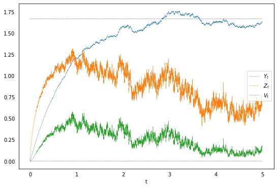
Figure 1. One trajectory for the processes $Y$, $Z$ and $V$.

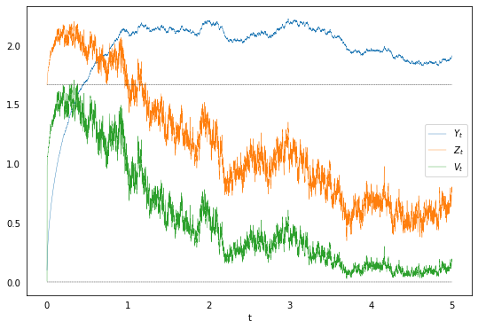
Figure 2. One trajectory for the processes $Y$, $Z$ and $V$.

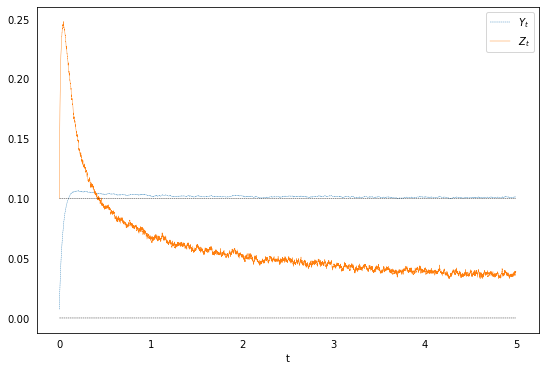
Figure 3. One trajectory for the processes $Y$, $Z$.

6. Conclusions

We have proposed a new family of stochastic models, based on Volterra SDEs of convolution type, which sheds some light in the modelling of the memory of a stochastic process. The key contribution of this approach is the two-sided explicit link that we are able to establish between a Volterra SDE of convolution type, with memory (the elephant process) and an associated standard SDE, without memory (the goldfish process).

On the numerical side, with particular reference to simulations via Euler scheme, the proposed approach is very promising, as we study the Euler scheme for both processes, the elephant and the goldfish, and we prove a strong error convergence rate of order $(\gamma\wedge\frac{1}{2})$, with $\gamma\in(0,1)$ depending on the regularity of the drift and volatility coefficients.

In particular, in the case of fractional convolution kernels parametrised by the Hurst coefficient $H$, the simulated trajectories display a rough behaviour, but nevertheless the corresponding numerical schemes do have a strong rate of convergence of order $\frac{1}{2}$ independently of the kernel, thus representing a remarkable improvement with respect to the order $H$ valid for standard Volterra equations.

This opens the door to numerous theoretical further investigations and to many applications, especially in mathematical finance, given the recent interest toward rough volatility modelling. First, one might ask what is a good financial model that could take advantage of the discovered Markov/non-Markov bridge of the transformation we proposed. Second, it would be worthwhile to study what numerical techniques are best for obtaining a performing technology in view of pricing derivative contracts, possibly including the powerful, versatile and elegant (stratified functional) quantization technique introduced in [10]. Indeed, quantization has already been successfully applied in the context of discretisation of SDEs [29], in particular for pricing in (Heston) stochastic volatility models [31] and, more recently in rough volatility models [5, 1], still for stratification purposes. In the third place, an analysis of the hedging problem and the computation of the Greeks, by possibly exploiting artificial intelligence techniques, is needed in order to assess the capability of the model at reproducing the market features and stylized facts.

Acknowledgements: The authors would like to thank Fabienne Comte and Andrea Pallavicini for fruitful discussions on the model and they thank all the participants to the Workshop “Volatility is rough: now what?”, and in particular E. Abi Jaber, C. Cuchiero, J. Guyon, A. Jacquier, M. Rosenbaum, for their precious comments and remarks.

The first author acknowledges financial support from the EPSRC grant EP/T032146/1. The fourth author acknowledges financial support from the chaire “Risques financiers” from the Fondation du Risque. Financial support has also been provided by the University of Padova grant BIRD227115 - "Equilibrium approaches in financial and energy markets".

Appendix A Basics on fractional integrals and Laplace transforms

A.1. Fractional integral and derivative

As a useful recap, we recall here the definition of Riemann-Liouville fractional integral and derivative, following [28, Chapter 2, Definition 2.1].

Definition A.1 (Fractional integral).

For $\beta>0$ and $f:(0,+\infty)\to\mathbb{R}$ in $L^{1}([0,T])$, the Riemann-Liouville fractional integral of order $\beta$ is defined as

$$I^{\beta}f(t)=\frac{1}{\Gamma(\beta)}\int_{0}^{t}(t-s)^{\beta-1}f(s)ds.$$ (A.1)

For simplicity, we skip $0$ in the above notation, so that to avoid writing $I_{0+}^{\beta}$.

Remark A.2.

Exploiting the fractional kernel $K_{\beta}$ introduced in Table 1 for $c=1$, we clearly have

$$I^{\beta}f(t)=(K_{\beta}\star f)(t).$$

Definition A.3 (Fractional derivative).

For $\beta\!\in(0,1)$, the Riemann-Liouville fractional derivative of order $\beta$ of $f$ reads

$$D^{\beta}f(t)=\frac{1}{\Gamma(1-\beta)}\frac{d}{dt}\int_{0}^{t}(t-s)^{-\beta}f(s)ds.$$ (A.2)

A sufficient condition for its existence is $f\in\textrm{AC}([0,T])$.

Remark A.4.

$(i)$ In this paper we deal with $\beta\in(0,1)$. Nevertheless, the fractional derivative is also defined for a general $\beta\geq 1$ as follows

$$D^{\beta}f(t)=\frac{1}{\Gamma(n-\beta)}\frac{d^{n}}{dt^{n}}\int_{0}^{t}(t-s)^{n-1-\beta}f(s)ds,\quad\mbox{ where }\quad n=\lfloor\beta\rfloor+1.$$ (A.3)

A sufficient condition for this to exist is $f\in\textrm{AC}^{\lfloor\beta\rfloor}([0,T])$.

$(ii)$ When $\beta=1$, $D^{\beta}$ coincides with the regular differentiation operator.

The following result, which corresponds to [28, Thm 2.4], might be useful as well.

Theorem A.5.

Let $\beta>0$. Then

$$D^{\beta}\circ I^{\beta}f=f$$ (A.4)

is true for any $f\in L^{1}([0,T])$. On the other hand, the equality

$$I^{\beta}\circ D^{\beta}f=f$$ (A.5)

is valid for $f\in\mathcal{I}^{\beta}(L^{1})$, where $\mathcal{I}^{\beta}(L^{1})$ denotes the space of functions $f$ that can be represented as the fractional integral of order $\beta$ of an integrable function, namely $f=I^{\beta}\varphi$ for some $\varphi\in L^{1}([0,T])$.

Direct computations allow to prove the next lemma [28, Section 2.3].

Lemma A.6.

Under Assumption 3.3, for every $\alpha,\beta>0$, we have the well-known composition formula:

$$I^{\beta}\circ I^{\alpha}f=I^{\alpha+\beta}f.$$ (A.6)

A.2. The Laplace transform as a useful tool

We briefly provide here some background on the Laplace transform, since it is a very efficient tool to deal with the key Equation  (3.1). Let us recall that the Laplace transform associated to (a kernel) $K$ always exists and reads, for $\zeta>0$

$$L_{K}(\zeta):=\int_{0}^{+\infty}e^{-\zeta u}K(u)du.$$ (A.7)

Exploiting the convolution Theorem [16, Theorem 2.8 $(iii)$],

$$L_{K}(\zeta)\cdot L_{\widetilde{K}}(\zeta)=L_{K\star\widetilde{K}}(\zeta),$$

and the injectivity of this transform, we obtain that Equation (3.1) reads, with $\rho>0$,

$$L_{K}(\zeta)\cdot L_{\widetilde{K}}(\zeta)=\int_{0}^{\infty}e^{-(\rho+\zeta)u}du=\frac{1}{\zeta+\rho},\text{ for all }\zeta>0$$ (A.8)

and this gives an easy way of finding $\widetilde{K}$, given $K$, as we are going to see below.

Example A.7.

When $K$ is the Gamma kernel $K_{c,\alpha,\rho}$ in Table 1, for $c>0,\alpha\in(0,1),\rho>0$, then, introducing $v=u(\zeta+\rho)$, we have

$$L_{K_{c,\alpha,\rho}}(\zeta)=\int_{0}^{\infty}ce^{-(\zeta+\rho)u}\frac{u^{\alpha-1}}{\Gamma(\alpha)}du=\frac{c(\zeta+\rho)^{-\alpha}}{\Gamma(\alpha)}\int_{0}^{\infty}e^{-v}v^{\alpha-1}dv=c(\zeta+\rho)^{-\alpha}.$$

It is then easy to see that $\widetilde{K}_{c,\alpha,\rho}=K_{\frac{1}{c},1-\alpha,\rho}$, namely

$$\widetilde{K}_{c,\alpha,\rho}(u)=K_{\frac{1}{c},1-\alpha,\rho}(u)=e^{-\rho u}K_{\frac{1}{c},1-\alpha,0}(u)=\frac{e^{-\rho u}}{c}\frac{u^{-\alpha}}{\Gamma(1-\alpha)}.$$

In the next final example we focus on the simpler case when $\rho=0$, i.e., when $(K\star\widetilde{K})=1$.

Example A.8 (The case $(K\star\widetilde{K})=1$).

We now deal with Equation (3.1) in the case $\rho=0$.

• For the constant kernel, $K(u)=c>0$ for all $u\in[0,T]$, we get $L_{K}(\zeta)=\frac{c}{\zeta}$ and so $L_{\widetilde{K}}(\zeta)\equiv 1/c$. In this case $\widetilde{K}$ only exists as a measure, namely $\widetilde{K}=\frac{1}{c}\delta_{0}$ (Dirac mass at $0$). Indeed (recall Remark 3.2) in this case $\widetilde{K}$ is the resolvent of the first kind of $K$.

• When $K$ is the fractional kernel $K_{c,\alpha,0}$ in Table 1, for $\alpha\in(0,1)$, this corresponds to $\alpha$-fractional integration since (see, e.g., [28, Eq. (7.5)])

  $$L_{K_{c,\alpha,0}}(\zeta)=c\int_{0}^{\infty}e^{-\zeta u}\frac{u^{\alpha-1}}{\Gamma(\alpha)}du=c\,\zeta^{-\alpha}.$$

  Then, $L_{\widetilde{K}_{c,\alpha,0}}(\zeta)=\frac{1}{c}\zeta^{-(1-\alpha)}$ and so, for $\alpha\in(0,1)$

  $$\widetilde{K}_{c,\alpha,0}=K_{\frac{1}{c},1-\alpha,0}.$$ (A.9)

Appendix B Proofs

B.1. Proof of Lemma 2.2

The proof exploits Kolmogorov continuity criterion (see e.g. [26, Theorem 3.23])

First of all, by interchanging the order of integration, we prove that the stochastic integral exists, since $\|X_{t}\|_{2}^{2}$ is finite for every $t\in[0,T]$. Indeed, we have

$$\|X_{t}\|_{2}^{2}=\mathbb{E}\left(\int_{0}^{t}K(t-s)Y_{s}dW_{s}\right)^{2} \leq \int_{0}^{t}K^{2}(u)du\cdot\sup_{t\in[0,T]}\mathbb{E}[Y_{t}^{2}]<+\infty,$$

where we have exploited Assumptions $i)-ii)$ on the convolution kernel and the fact that $\beta>1$. Moreover, for $0\leq s\leq t$, exploiting BDG inequality and the generalized Minkowski inequality with $r=2$ and $p\geq 2$, we obtain

$$\Big{|}\Big{|}\int_{0}^{t}K(t-u) Y_{u}dW_{u}-\int_{0}^{s}K(s-u)Y_{u}dW_{u}\Big{|}\Big{|}_{p}$$

$$\leq\Big{|}\Big{|}\int_{0}^{s}\left(K(t-u)-K(s-u)\right)Y_{u}dW_{u}\Big{|}\Big{|}_{p}+\Big{|}\Big{|}\int_{s}^{t}K(t-u)Y_{u}dW_{u}\Big{|}\Big{|}_{p}$$

$$\leq C_{p}^{\textrm{BDG}}\Big{\{}\Big{|}\Big{|}\left(\int_{0}^{s}\left(K(t-u)-K(s-u)\right)^{2}Y_{u}^{2}du\right)^{\frac{1}{2}}\Big{|}\Big{|}_{p}+\Big{|}\Big{|}\left(\int_{s}^{t}K^{2}(t-u)Y_{u}^{2}du\right)^{\frac{1}{2}}\Big{|}\Big{|}_{p}\Big{\}}$$

$$\stackrel{{\scriptstyle p\geq 2}}{{\leq}}C_{p}^{\textrm{BDG}}\Big{\{}\left(\int_{0}^{s}\left(K(t-u)-K(s-u)\right)^{2}\big{|}\big{|}Y_{u}\big{|}\big{|}_{p}^{2}du\right)^{\frac{1}{2}}+\left(\int_{s}^{t}K^{2}(t-u)\big{|}\big{|}Y_{u}\big{|}\big{|}_{p}^{2}du\right)^{\frac{1}{2}}\Big{\}}$$

$$\leq C_{p}^{\textrm{BDG}}\sup_{u\in[0,T]}\big{|}\big{|}Y_{u}\big{|}\big{|}_{p}\Big{\{}\left(\int_{0}^{s}\left(K(t-u)-K(s-u)\right)^{2}du\right)^{\frac{1}{2}}+\left(\int_{s}^{t}K^{2}(t-u)du\right)^{\frac{1}{2}}\Big{\}}.$$

Hence, by two elementary changes of variable we obtain

$$\Big{|}\Big{|}\int_{0}^{t} K(t-u)Y_{u}dW_{u}-\int_{0}^{s}K(s-u)Y_{u}dW_{u}\Big{|}\Big{|}_{p}$$

$$\leq C_{p}^{\textrm{BDG}}\sup_{u\in[0,T]}\big{|}\big{|}Y_{u}\big{|}\big{|}_{p}\Big{\{}\left(\int_{0}^{s}\left(K(t-s+v)-K(v)\right)^{2}du\right)^{\frac{1}{2}}+\left(\int_{0}^{t-s}K^{2}(v)dv\right)^{\frac{1}{2}}\Big{\}}$$ (B.1)

$$\leq C_{p}^{\textrm{BDG}}C_{K}(t-s)^{\theta}.$$

where, in the last step, we have used Assumption $iv)$.

B.2. Proof of Theorem 3.4.

We split the proof into three steps: we first deal with the Markovian stochastic process $\xi$, we then deal with $X$ and finally we prove the equation linking them.

Step 1. The diffusion SDE in Equation (3.6). This SDE can be rewritten as follows. We set $\widetilde{\kappa}(t):=e^{\rho t}(\widetilde{K}\star\mbox{\bf 1})(t)=e^{\rho t}\widetilde{\varphi}(t)$, with $\widetilde{\varphi}(t)=(\widetilde{K}\star\mbox{\bf 1})(t)$, and we define $(\mathbb{Y}_{t})_{t\in[0,T]}$ as

$$\mathbb{Y}_{t}:=(Y^{1}_{t},Y^{2}_{t}):=(\xi^{0},\xi_{t}-\widetilde{\kappa}(t)\xi^{0}),\quad t\!\in[0,T],$$

so that

$$\xi_{t}=Y_{t}^{2}+\widetilde{\kappa}(t)Y_{t}^{1}=Y_{t}^{2}+\widetilde{\kappa}(t)\xi^{0}.$$

Then, for $t\in[0,T]$, $(\mathbb{Y}_{t})_{t\in[0,T]}$ satisfies a SDE that component-wise reads as

$$Y^{1}_{t} =\xi^{0}+\int_{0}^{t}0\,ds+\int_{0}^{t}0\;dW_{s},$$ (B.2)

$$Y^{2}_{t} =\int_{0}^{t}\widetilde{b}(s,Y^{2}_{s}+\widetilde{\kappa}(s)Y_{s}^{1})ds+\int_{0}^{t}\widetilde{\sigma}(s,Y^{2}_{s}+\widetilde{\kappa}(s)Y^{1}_{s})dW_{s},$$ (B.3)

or, equivalently,

$$d\mathbb{Y}_{t}=\overline{b}(t,\mathbb{Y}_{t})dt+\overline{\sigma}(t,\mathbb{Y}_{t})dW_{t},\quad\mathbb{Y}_{0}=\begin{pmatrix}\xi^{0}\\ 0\end{pmatrix},$$ (B.4)

with

$$\overline{b}\big{(}t,(y^{1},y^{2})\big{)}=\begin{pmatrix}0\\ \widetilde{b}(t,y^{2}+\widetilde{\kappa}(t)y^{1})\end{pmatrix}\quad\mbox{ and }\quad\overline{\sigma}(t,(y^{1},y^{2})):=\begin{pmatrix}0\\ \widetilde{\sigma}(t,y^{2}+\widetilde{\kappa}(t)y^{1})\end{pmatrix}.$$ (B.5)

Now, by condition (b)), $b$ and $\sigma$ are Lipschitz continuous in $x$ uniformly in $t\!\in[0,T]$, so that $\widetilde{b}(t,x)$ and $\widetilde{\sigma}(t,x)$, defined by (3.7) clearly satisfy the same assumption with

$$[\widetilde{b}]_{{\rm Lip},x}\leq e^{\rho T}[b]_{{\rm Lip},x}\quad\mbox{ and }\quad[\widetilde{\sigma}]_{{\rm Lip},x}\leq e^{\rho T}[\sigma]_{{\rm Lip},x},$$

and

$$\sup_{t\in[0,T]}(|\widetilde{\sigma}(t,0)|+|\widetilde{b}(t,0)|)\leq e^{\rho T}\sup_{t\in[0,T]}(|\sigma(t,0)|+|b(t,0)|)<+\infty.$$

So, as a third sub-step, one easily checks that $\overline{b}$ and $\overline{\sigma}$ introduced in Equation (B.5) are Borel on $[0,T]\times\mathbb{R}$. Furthermore, they satisfy a $2$-dimensional version of the Lipschitz assumption in Equation  (b)) in $\mathbf{y}=(y^{1},y^{2})$, uniformly in $t\!\in[0,T]$ since $\widetilde{\kappa}$ is non-negative and non-decreasing with $\widetilde{\kappa}(T)<+\infty$, by definition. Indeed, by introducing $\mathbf{y}:=(y^{1},y^{2})$ and $\mathbf{y}^{\prime}:=({(y^{1})}^{\prime},{(y^{2})}^{\prime})$ we have

$$\|\overline{b}\big{(}t,\mathbf{y}\big{)}-\overline{b}\big{(}t,\mathbf{y}^{\prime}\big{)}\| =\big{|}\widetilde{b}\left(t,y^{2}+\widetilde{\kappa}(t)y^{1}\right)-\widetilde{b}\left(t,{(y^{2})}^{\prime}+\widetilde{\kappa}(t){(y^{1})}^{\prime}\right)\big{|}$$

$$\leq[\widetilde{b}]_{{\rm Lip},x}\left(\big{|}y^{2}-{(y^{2})}^{\prime}\big{|}+\widetilde{\kappa}(T)\big{|}y^{1}-{(y^{1})}^{\prime}\big{|}\right)$$

$$\leq[\widetilde{b}]_{{\rm Lip},x}(1\vee\widetilde{\kappa}(T))\left(\big{|}y^{2}-{(y^{2})}^{\prime}\big{|}+\big{|}y^{1}-{(y^{1})}^{\prime}\big{|}\right)$$

$$=[\widetilde{b}]_{{\rm Lip},x}(1\vee\widetilde{\kappa}(T))\|\mathbf{y}-\mathbf{y}^{\prime}\|_{1}\leq\sqrt{2}[\widetilde{b}]_{{\rm Lip},x}(1\vee\widetilde{\kappa}(T))\|\mathbf{y}-\mathbf{y}^{\prime}\|_{2},$$

where $||\cdot||_{1}$ and $||\cdot||_{2}$ denote, respectively, the $L^{1}$ and the $L^{2}$ norms of a real vector and the same holds for $\overline{\sigma}$. Moreover,

$$\sup_{t\in[0,T]}\|\overline{b}(t,0)\|+\|\overline{\sigma}(t,0)\| \leq\sup_{t\in[0,T]}|\widetilde{b}(t,0)|+|\widetilde{\sigma}(t,0)|<+\infty,$$

and so the above $2$-dimensional SDE (B.4) has a unique pathwise continuous, $\mathbb{F}^{\xi^{0},W}$-adapted solution starting from $\mathbb{Y}_{0}$ (see [33, Thm. IX.2.1] and [8, Theorem A3.3, Chapter 5] among others). This in turn implies that the same holds for Equation (3.6).

Moreover, the regularity of $\overline{b}$ and $\overline{\sigma}$ above implies that, for some positive constant $C>0$,

$$\sup_{t\in[0,T]}\|\overline{b}(t,\mathbf{y})\|+\|\overline{\sigma}(t,\mathbf{y})\|\leq C(1+\|\mathbf{y}\|_{2})$$

so that, by [30, Prop. 7.6 $(a)$], the following moment estimate holds, for every $p\!\in(0,+\infty)$,

$$\Big{\|}\sup_{t\in[0,T]}\|\mathbb{Y}_{t}\|\Big{\|}_{p}\leq C_{\widetilde{b},\widetilde{\sigma},T,p}(1+\|\mathbb{Y}_{0}\|_{p}),$$ (B.6)

where $C_{\widetilde{b},\widetilde{\sigma},T,p}>0$. Hence, using that $X_{t}=Y^{2}_{t}+\widetilde{\kappa}(t)\xi^{0}$, we immediately derive

$$\sup_{t\in[0,T]}|\xi_{t}|\leq\sup_{t\in[0,T]}|Y_{t}^{2}|+\widetilde{\kappa}(T)|\xi^{0}|$$

which finally implies

$$\Big{\|}\sup_{t\in[0,T]}|\xi_{t}|\Big{\|}_{p}\leq C^{\prime}_{b,\sigma,T,p}(1+\|\xi^{0}\|_{p}).$$ (B.7)

Moreover, as $\mathbb{Y}$ is an Itô process with continuous integrands, by localization and Kolmogorov’s criterion one classically shows that it has pathwise $a$-Hölder paths for every $a\!\in(0,1/2)$, up to $\mathbb{P}$-indistinguishability. As consequence $\xi_{t}=Y^{2}_{t}-\widetilde{\kappa}(t)$ acquires the lowest pathwise regularity between the one of $Y^{2}$ and $\widetilde{\varphi}$, so that, if $\widetilde{\varphi}$ is $\eta$-Hölder continuous for some $\eta\!\in(0,\frac{1}{2})$, then $\xi$ is $(a\wedge\eta)$-Hölder continuous.

Step 2. The SDE in Equation (3.3). We rewrite Equation (3.3) as

$$X_{t}=\xi^{0}+\int_{0}^{t}K(t-s)b(s,e^{-\rho s}\xi_{s})ds+\int_{0}^{t}K(t-s)\sigma(s,e^{-\rho s}\xi_{s})dW_{s},$$ (B.8)

where $\xi_{t}=Y^{2}_{t}+\tilde{\kappa}(t)$ with $Y^{2}$ pathwise continuous. Let us notice that the terms on the right hand side of the above equation exist for every $t\!\in[0,T]$, since both $s\mapsto b(s,e^{-\rho s}\xi_{s})$ and $s\mapsto\sigma(s,e^{-\rho s}\xi_{s})$ are pathwise continuous (and ${\mathbb{F}}^{\xi^{0},W}$-adapted) and satisfy

$$\int_{0}^{t}\left[K(t-s)|b(s,e^{-\rho s}\xi_{s})|+K(t-s)^{2}\sigma(s,e^{-\rho s}\xi_{s})^{2}\right]ds\leq C_{b,\sigma,\rho,T}(1+\sup_{s\in[0,T]}|\xi_{s}|^{2})<+\infty,\;\quad\mathbb{P}\text{-a.s.}$$

since $\int_{0}^{T}K(s)^{2}ds<+\infty$. This defines $X_{t}$ for every $t\!\in[0,T]$. Now, let us prove the existence of a continuous modification of $X$, starting with the case of $\xi^{0}\!\in L^{p}(\mathbb{P})$, for $p$ large enough. We proved in Step 1 that $\mathbb{Y}$, and so $\xi$, have a pathwise continuous modification that we consider in what follows. Then, the drift term $\int_{0}^{t}K(t-s)b(s,e^{-\rho s}\xi_{s})ds=\int_{0}^{t}K(s)b(s,e^{-\rho(t-s)}\xi_{t-s})ds$ is continuous by standard elementary arguments. As for the stochastic integral term, we first rely on Lemma 2.2. It follows from Equations (B.7) and (b)) that

$$\sup_{t\in[0,T]}\big{\|}\sigma(t,e^{-\rho t}\xi_{t})\big{\|}_{p}<+\infty.$$

Then, it follows from Lemma 2.2 that the stochastic integral process $t\mapsto\int_{0}^{t}K(t-s)\sigma(s,e^{-\rho s}\xi_{s})dW_{s}$ has a pathwise continuous, more precisely $\gamma$-Hölder continuous, modification for any $\gamma\in\left(0,(\theta\wedge\frac{\beta-1}{2\beta})-\frac{1}{p}\right)$ owing to the integrability assumption c), $\xi^{0}\!\in L^{p}(\mathbb{P})$, for some $p>\max\left\{\frac{1}{\theta\wedge\frac{\beta-1}{2\beta}},2\right\}$. Finally, $X$ also has a pathwise continuous modification.

Assume, now, $p\!\in(0,+\infty)$. Let us define the $\sigma(\xi^{0})$-measurable events $A_{k}=\{k\leq|\xi^{0}|\leq k+1\}$, $k\geq 0$ and let $X^{(k)}$ be defined by (B.8) starting from $(\xi^{0})^{(k)}=\xi^{0}\mbox{\bf 1}_{\{k\leq|\xi^{0}|<k+1\}}=\xi^{0}\mbox{\bf 1}_{A_{k}}$ where $\xi$ is replaced by the solution $\xi^{(k)}$ to (3.6) starting from $(\xi^{0})^{(k)}$. It follows from the fact that $\mathcal{F}^{\xi^{0},W}_{0}\supset\sigma(\xi^{0})$ and that any $\mathcal{F}^{\xi^{0},W}_{0}$-measurable random variable commutes with stochastic integrals with respect to the Brownian motion $W$, i.e. $\mbox{\bf 1}_{A}\int_{0}^{t}H_{s}dW_{s}=\int_{0}^{t}\mbox{\bf 1}_{A}H_{s}dW_{s}$ for any $A\!\in\sigma(\xi^{0})$ (independent of $W$) and that $\xi=\xi^{(k)}$ on $A_{k}$, $k\geq 0$ (due to the same “local” feature of stochastic integration) that $\xi^{(k)}$ is solution to the original Equation (B.8) on $A_{k}$. Moreover, as $(\xi^{0})^{(k)}$ lies in every $L^{p}(\mathbb{P})$, $p>0$, it follows from what precedes that $\xi^{(k)}$ has a $a$-Hölder continuous modification for any $a\!\in\left(0,(\theta\wedge\frac{\beta-1}{2\beta})\right)$. As a consequence, the process $X$ defined by

$$X_{t}=\sum_{k\geq 0}\mbox{\bf 1}_{A_{k}}X^{(k)}_{t},\quad t\!\in[0,T],$$

is solution to Equation (B.8) with $\gamma$-Hölder regularity, for any $a\!\in\left(0,(\theta\wedge\frac{\beta-1}{2\beta})\right)$, regardless of the integrability of $\xi^{0}$. Following the same reasoning as in [24, Appendix C], one concludes by noting that, as $(\xi^{0})^{(k)}$ is bounded and consequently lies in all $L^{p}(\mathbb{P})$ spaces, $X^{(k)}$ has a pathwise continuous modification and so has $X$.

Step 3. Final step. One takes advantage of the properties enjoyed by $X$ and $\xi$ to prove that $e^{\rho\cdot}(\widetilde{K}\star X$) is a solution to Equation (3.6), i.e., equal to $\xi$ (by uniqueness of the strong solution of Equation (3.6)). Uniqueness of $X$ follows by the same reasoning used in the previous steps, so that everything is rigorous as for strong solutions.

Moreover,

$$K\star(e^{-\rho\cdot}\xi)=K\star(\widetilde{K}\star X)=(K\star\widetilde{K})\star X=e^{-\rho\cdot}\star X=e^{-\rho\cdot}\int_{0}^{\cdot}e^{\rho s}X_{s}ds.$$

On the other hand, one checks that $e^{\rho\cdot}\big{(}K\star(e^{-\rho\cdot}\xi)\big{)}=(Ke^{\rho\cdot})\star\xi$ so that

$$\int_{0}^{t}e^{\rho s}X_{s}ds=\big{(}(Ke^{\rho\cdot})\star\xi\big{)}_{t}$$

or, equivalently, since $X$ is pathwise continuous,

$$X_{t}=e^{-\rho t}\frac{d}{dt}\big{(}(Ke^{\rho\cdot})\star\xi\big{)}_{t}$$

and the conclusion follows.

B.3. Proof of Theorem 4.1

In the computations that follow, the constants $C_{b,\sigma,T,p}$ may vary from line to line but they do not depend neither on the step of the schemes, nor on the (pseudo-)starting value $\xi^{0}$. The proof is divided into three steps: in the first one, in Equation (B.9), we establish uniform bounds for the solutions of the SDE and of its Euler schemes. In the second step, for $p\geq 2$, the strong error rate for the Euler scheme is proved, with the difficulty of dealing with the non-null initial condition. In the third and final step we treat the case $p\in(0,2)$.

Step 1: Recall that $\mathbb{Y}$, defined in the proof of Theorem 3.4 as (here $\widetilde{\kappa}(t)=\widetilde{\varphi}(t)$ as $\rho=0$)

$$\mathbb{Y}_{t}=(Y^{1}_{t},Y^{2}_{t}):=(\xi^{0},\xi_{t}-\widetilde{\varphi}(t)\xi^{0}),\quad t\!\in[0,T],$$

is solution to the regular SDE

$$d\mathbb{Y}_{t}=\overline{b}(t,\mathbb{Y}_{t})dt+\overline{\sigma}(t,\mathbb{Y}_{t})dW_{t},\quad\mathbb{Y}_{0}=\begin{pmatrix}\xi^{0}\\ 0\end{pmatrix},$$

with drift and diffusion coefficients which are Lipschitz in space, uniformly in time,

$$\overline{b}\big{(}t,(y^{1},y^{2})\big{)}=\begin{pmatrix}0\\ \widetilde{b}(t,y^{2}+\widetilde{\varphi}(t)y^{1})\end{pmatrix}\quad\mbox{ and }\quad\overline{\sigma}(t,(y^{1},y^{2})):=\begin{pmatrix}0\\ \widetilde{\sigma}(t,y^{2}+\widetilde{\varphi}(t)y^{1})\end{pmatrix}.$$

Exploiting [30, Proposition 7.2], we have, denoting by $\overline{\mathbb{Y}}^{h}=(\overline{Y}_{t}^{h,1},\overline{Y}_{t}^{h,2})$ the continuous time Euler scheme of $\mathbb{Y}$ with time step $h=\frac{T}{n}$,

$$\Big{\|}\sup_{t\in[0,T]}|\mathbb{Y}_{t}|\Big{\|}_{p}+\Big{\|}\sup_{t\in[0,T]}|\overline{\mathbb{Y}}^{h}_{t}|\Big{\|}_{p}\leq C_{b,\sigma,T,p}(1+\|\mathbb{Y}_{0}\|_{p})$$

where $C_{b,\sigma,T,p}$ is a real constant not depending on $n$, i.e., on the step $h$. We know that, by definition, $\mathbb{Y}=(\xi^{0},\xi_{t}-\widetilde{\varphi}(t)\xi^{0})$ and we straightforwardly check that for every step $h$

$$\overline{\xi}_{t}^{h}=\overline{\mathbb{Y}}_{t}^{h,2}+\widetilde{\varphi}(t)\xi^{0},\quad t\!\in[0,T].$$

Proceeding similarly as in the proof of Theorem 3.4 and exploiting the properties of $\widetilde{\varphi}$, namely $\widetilde{\varphi}(0)=0$ and $\widetilde{\varphi}$ non-decreasing, we also have that, for every $p>0$, there exists a a real constant $C_{b,\sigma,T,p}>0$ such that, for all $n\geq 1$ and $h=\tfrac{T}{n}$,

$$\Big{\|}\sup_{t\in[0,T]}|\xi_{t}|\Big{\|}_{p}+\Big{\|}\sup_{t\in[0,T]}|\overline{\xi}^{h}_{t}|\Big{\|}_{p}\leq C_{b,\sigma,T,p}(1+\|\xi^{0}\|_{p}).$$ (B.9)

Step 2. Now, let us assume $p\geq 2$. We first notice that, for a standard diffusion (e.g., if $\widetilde{\varphi}={\bf 1}$), from Equations (4.1) and (4.2), one has

$$\xi_{t}-\overline{\xi}_{t}=\int_{0}^{t}\big{(}b(s,\xi_{s})-b(\underline{s},\overline{\xi}_{\underline{s}})\big{)}ds+\int_{0}^{t}\big{(}\sigma(s,\xi_{s})-\sigma(\underline{s},\overline{\xi}_{\underline{s}})\big{)}dW_{s}.$$ (B.10)

Then, we follow the lines of the proof of [30, Theorem 7.2, Section 7.8.4, p.331], which is based on Burkholder-Davis-Gundy (BDG), generalized Minkowski inequalities and a variant of Gronwall’s lemma  [30, Lemma 7.3, p.327], and we apply them on the decomposition

$$\xi_{s}-\overline{\xi}_{\underline{s}}=\xi_{s}-\xi_{\underline{s}}+\xi_{\underline{s}}-\overline{\xi}_{\underline{s}},\quad s\!\in[0,T],$$

exploiting the obvious fact that $\sup_{s\in[0,T]}\|\xi_{\underline{s}}-\overline{\xi}_{\underline{s}}\|_{p}\leq\sup_{s\in[0,T]}\|\xi_{s}-\overline{\xi}_{s}\|_{p}$. Then we derive, using the (uniform in time) Lipschitz condition from Equation (4.3),

$$\forall\,t\!\in[0,T],\quad\Big{\|}\sup_{s\in[0,t]}|\xi_{s}-\overline{\xi}_{s}|\Big{\|}_{p}\leq C_{b,\sigma,T,p}\Bigg{(}h^{\gamma}(1+\|\xi^{0}\|_{p})+\int_{0}^{t}\|\xi_{s}-\xi_{\underline{s}}\|_{p}ds+\Big{(}\int_{0}^{t}\|\xi_{s}-\xi_{\underline{s}}\|_{p}^{2}ds\Big{)}^{1/2}\Bigg{)}.$$ (B.11)

The process $(\Lambda_{t})_{t\in[0,T]}$ defined by

$$\Lambda_{t}:=\int_{0}^{t}b(s,\xi_{s})ds+\int_{0}^{t}\sigma(s,\xi_{s})dW_{s},\quad t\!\in[0,T],$$

is an Itô process such that $\big{\|}\sup_{t\in[0,T]}|b(t,\xi_{t})|\big{\|}_{p}+\big{\|}\sup_{t\in[0,T]}|\sigma(t,\xi_{t})|\big{\|}_{p}\leq C_{b,\sigma,T,p}(1+\|\xi^{0}\|)_{p}$, owing to Equations (4.3) and (B.9). Consequently, from [30, Lemma 7.4, Section 7.8.3, p.329], it follows

$$\Big{\|}\Lambda_{t}-\Lambda_{s}\Big{\|}_{p}\leq C_{b,\sigma,T,p}|t-s|^{1/2}(1+\|\xi^{0}\|_{p}).$$

Then, noticing that

$$\xi_{t}-\xi_{\underline{t}}=\xi^{0}(\widetilde{\varphi}(t)-\widetilde{\varphi}(\underline{t})\big{)}+\Lambda_{t}-\Lambda_{\underline{t}}$$

and since $\widetilde{\varphi}$ is non-decreasing, we find

$$\|\xi_{t}-{\xi}_{\underline{t}}\|_{p}\leq\|\xi^{0}\|_{p}\big{(}\widetilde{\varphi}(t)-\widetilde{\varphi}(\underline{t})\big{)}+C_{b,\sigma,T,p}\cdot h^{1/2}\big{(}1+\|\xi^{0}\|_{p}\big{)}.$$ (B.12)

Plugging this inequality into (B.11) yields

$$\Big{\|}\sup_{t\in[0,T]}|\xi_{t}-\overline{\xi}_{t}|\Big{\|}_{p} \leq C_{b,\sigma,T,p}\Bigg{(}h^{\frac{1}{2}\wedge\gamma}(1+\|\xi^{0}\|_{p})+\int_{0}^{T}\big{(}\widetilde{\varphi}(t)-\widetilde{\varphi}(\underline{t})\big{)}dt+\Big{(}\int_{0}^{T}\big{(}\widetilde{\varphi}(t)-\widetilde{\varphi}(\underline{t})\big{)}^{2}dt\Big{)}^{1/2}\Bigg{)}$$

$$\leq C_{b,\sigma,T,p}\Bigg{(}h^{\frac{1}{2}\wedge\gamma}(1+\|\xi^{0}\|_{p})+(1+\sqrt{T})\Big{(}\int_{0}^{T}\big{(}\widetilde{\varphi}(t)-\widetilde{\varphi}(\underline{t})\big{)}^{2}dt\Big{)}^{1/2}\Bigg{)},$$ (B.13)

where we used the elementary inequality $\sqrt{a+b}\leq\sqrt{a}+\sqrt{b}$, for $a$, $b\geq 0$ in the first line and Cauchy-Schwartz inequality in the second one. As $\widetilde{\varphi}$ is non-decreasing and concave, for every $t\!\in(0,T]$, we have

$$0\leq\widetilde{\varphi}(t)-\widetilde{\varphi}(\underline{t})\leq\widetilde{\varphi}^{\prime}_{r}(\underline{t})(t-\underline{t})$$

where $\widetilde{\varphi}^{\prime}_{r}$ is the right derivative of $\widetilde{\varphi}$ on $(0,T]$. Let us notice that $\widetilde{\varphi}^{\prime}_{r}(0)$ exists but it can be equal to $+\infty$. Consequently, as $\underline{t}=0$ if $t\in[0,\frac{T}{n})$ and $\widetilde{\varphi}(0)=0$, we obtain

$$\int_{0}^{T}\big{(}\widetilde{\varphi}(t)-\widetilde{\varphi}(\underline{t})\big{)}^{2}dt \leq\int_{0}^{\tfrac{T}{n}}\widetilde{\varphi}^{2}(t)dt+\int_{\frac{T}{n}}^{T}(\varphi_{r}^{\prime}(\underline{t}))^{2}(t-\underline{t})^{2}dt\leq\tfrac{T}{n}\widetilde{\varphi}^{2}\big{(}\tfrac{T}{n}\big{)}+\sum_{k=1}^{n-1}\int_{\frac{kT}{n}}^{\frac{(k+1)T}{n}}(\widetilde{\varphi}_{r}^{\prime}\big{(}\tfrac{kT}{n}\big{)})^{2}\big{(}t-\tfrac{kT}{n}\big{)}^{2}dt$$

$$\leq\tfrac{T}{n}\Big{(}\widetilde{\varphi}^{2}\big{(}\tfrac{T}{n}\big{)}+\big{(}\tfrac{T}{n}\big{)}^{2}\sum_{k=1}^{n-1}(\widetilde{\varphi}_{r}^{\prime}\big{(}\tfrac{kT}{n}\big{)})^{2}\Big{)}.$$

Hence, the fact that $(\sum_{i}a_{i}^{2})^{1/2}\leq\sum_{i}a_{i}$, for $a_{i}\geq 0$, together with the fact that $\widetilde{\varphi}_{r}^{\prime}$ is non-increasing by concavity of $\widetilde{\varphi}$ yield

$$\left(\int_{0}^{T}\big{(}\widetilde{\varphi}(t)-\widetilde{\varphi}(\underline{t})\big{)}^{2}ds\right)^{1/2} \leq\sqrt{\tfrac{T}{n}}\Big{(}\widetilde{\varphi}\big{(}\tfrac{T}{n}\big{)}+\tfrac{T}{n}\sum_{k=1}^{n-1}\widetilde{\varphi}_{r}^{\prime}\big{(}\tfrac{kT}{n}\big{)}\Big{)}\leq\sqrt{\tfrac{T}{n}}\Big{(}\widetilde{\varphi}\big{(}\tfrac{T}{n}\big{)}+\int_{0}^{\frac{(n-1)T}{n}}\widetilde{\varphi}^{\prime}_{r}(t)dt\Big{)}$$

$$\leq 2\,\widetilde{\varphi}\big{(}T\big{)}\sqrt{\tfrac{T}{n}}.$$ (B.14)

One concludes that, for every step $h$,

$$\Big{\|}\sup_{t\in[0,T]}|\xi_{t}-\overline{\xi}_{t}|\Big{\|}_{p}\leq C_{b,\sigma,T,p}\,h^{\frac{1}{2}\wedge\gamma}(1+\|\xi^{0}\|_{p}).$$

Step 3. Now, let us consider $0<p<2$. There exist functionals $F$ and $\overline{F}:\mathbb{R}\times C([0,T],\mathbb{R})\to C([0,T],\mathbb{R})$ such that

$$\xi=F(\xi^{0},\mathcal{W})\quad\mbox{ and }\quad\overline{\xi}=\overline{F}(\xi^{0},\mathcal{W}).$$

This is a straightforward consequence of Blagoven$\check{{\rm s}}\check{{\rm c}}$enkii-Freidlin Theorem [35, Theorem V.13.1] applied to $\mathbb{Y}$ and the fact that $\xi=Y^{2}+\widetilde{\varphi}(\cdot)\xi^{0}$ and $\overline{\xi}=\overline{Y}^{2}-\widetilde{\varphi}(\cdot)\xi^{0}$. Then, temporarily denoting by $\xi^{(x_{0})}$ and $\overline{\xi}^{(x_{0})}$ the process $\xi$ and its Euler scheme, respectively, starting at $\xi^{0}=x_{0}$, we obtain

$$\int\sup_{t\in[0,T]}|\xi_{t}-\overline{\xi}_{t}|^{p}d\mathbb{P} =\int\mathbb{E}\left(\sup_{t\in[0,T]}|\xi^{(x_{0})}_{t}-\overline{\xi}^{(x_{0})}_{t}|^{p}\right)d\mathbb{P}_{\xi^{0}}(x_{0})\leq\int\left[\mathbb{E}\left(\sup_{t\in[0,T]}|\xi^{(x_{0})}_{t}-\overline{\xi}^{(x_{0})}_{t}|^{2}\right)\right]^{\frac{p}{2}}d\mathbb{P}_{\xi^{0}}(x_{0})$$

$$\leq(C_{b,\sigma,T,2})^{p}\int(1+|\xi^{0}|)^{p}d\mathbb{P}_{\xi^{0}}(x_{0})\leq 2^{p}(C_{b,\sigma,T,2})^{p}(1+\mathbb{E}|\xi^{0}|^{p}),$$

so that

$$\Big{\|}\sup_{t\in[0,T]}|\xi_{t}-\overline{\xi}_{t}|\Big{\|}_{p}\leq 2\,C_{b,\sigma,T,2}\,h^{\frac{1}{2}\wedge\gamma}(1+\|\xi^{0}\|_{p}).$$

This completes the proof.

B.4. Proof of Corollary 4.2

Let us temporarily assume $p\geq 1$, so that $\|\cdot\|_{p}$ is a norm. One has, for every $t\!\in[0,T]$,

$$\|\xi_{t}-\overline{\xi}_{\underline{t}}\|_{p} \leq\|\xi_{t}-\xi_{\underline{t}}\|_{p}+\|\xi_{\underline{t}}-\overline{\xi}_{\underline{t}}\|_{p}\leq\|\xi_{t}-\xi_{\underline{t}}\|_{p}+\Big{\|}\sup_{t\in[0,T]}\big{|}\xi_{\underline{t}}-\overline{\xi}_{\underline{t}}\big{|}\Big{\|}_{p}.$$

Hence, for every $r>0$, we get

$$\left(\int_{0}^{T}\|\xi_{t}-\overline{\xi}_{\underline{t}}\|^{r}_{p}dt\right)^{1/r}\leq 2^{(r-1)^{+}}\left(\Big{(}\int_{0}^{T}\|\xi_{t}-\xi_{\underline{t}}\|^{r}_{p}dt\Big{)}^{1/r}+T^{1/r}\Big{\|}\sup_{t\in[0,T]}\big{|}\xi_{t}-\overline{\xi}_{t}\big{|}\Big{\|}_{p}\right).$$

Finally, one relies on Equation (B.12) and Theorem 4.1 to provide upper-bounds for the first and the second term on the right hand side of the above inequality, respectively, to get

$$\left(\int_{0}^{T}\|\xi_{t}-\overline{\xi}_{\underline{t}}\|^{r}_{p}dt\right)^{1/r}\leq C_{b,\sigma,T,p,r}(1+\|\xi^{0}\|_{p})\left(\Big{(}\frac{T}{n}\Big{)}^{\gamma\wedge\frac{1}{2}}+\Big{(}\int_{0}^{T}(\widetilde{\varphi}(t)-\widetilde{\varphi}(\underline{t}))^{r}dt\Big{)}^{1/r}\Big{)}\right).$$

If $0<p<1$, one gets analogous results (with different constants) using the sub-additivity of $\|\cdot\|_{p}$.

B.5. Proof of Theorem 4.4

The proof is split into two steps: the first dealing with the case $p\geq 2$ and the second with the case $p\in(0,2)$.

Step 1 (Case $p\geq 2$). We start by considering the following equation

$$X_{t}=\xi^{0}+\int_{0}^{t}K(t-s)\big{(}b(s,\xi_{s})ds+\sigma(s,\xi_{s})dW_{s}\big{)}$$

and its Euler like (continuous time) discretization with time step $h=\frac{T}{n}$, defined by

$$\overline{X}_{t}=\xi^{0}+\int_{0}^{t}K(t-s)\big{(}b(\underline{s},\overline{\xi}_{\underline{s}})ds+\sigma(\underline{s},\overline{\xi}_{\underline{s}})dW_{s}\big{)}.$$

Then, by a standard application of BDG inequality and generalized Minkowski inequality, we have, for $p\geq 2$,

$$\|X_{t}-\overline{X}_{t}\|_{p} \leq\int_{0}^{t}K(t-s)\|b(s,\xi_{s})-b(\underline{s},\overline{\xi}_{\underline{s}})\|_{p}ds+C^{BDG}_{p}\left(\int_{0}^{t}K(t-s)^{2}\|\sigma(s,\xi_{s})-\sigma(\underline{s},\overline{\xi}_{\underline{s}})\|^{2}_{p}ds\right)^{1/2}$$

$$\leq[b]_{HolLip}\int_{0}^{t}K(t-s)\big{(}(s-\underline{s})^{\gamma}+\big{\|}\xi_{s}-\overline{\xi}_{\underline{s}}\big{\|}_{p}\big{)}ds$$

$$\qquad+C^{BDG}_{p}[\sigma]_{HolLip}\left(\int_{0}^{t}K(t-s)^{2}\big{(}(s-\underline{s})^{2\gamma}+\big{\|}\xi_{s}-\overline{\xi}_{\underline{s}}\big{)}\big{\|}^{2}_{p}\big{)}ds\big{)}\right)^{1/2}.$$

Using the elementary inequality $\sqrt{a+b}\leq\sqrt{a}+\sqrt{b}$, for $a,\,b\geq 0$, we obtain

$$\|X_{t}-\overline{X}_{t}\|_{p} \leq\left([b]_{HolLip}\int_{0}^{T}K(s)ds+C^{BDG}_{p}[\sigma]_{HolLip}\left(\int_{0}^{T}K(s)^{2}ds\right)^{1/2}\right)\Big{(}\frac{T}{n}\Big{)}^{\gamma}$$

$$\quad+[b]_{HolLip}\int_{0}^{t}K(t-s)\big{\|}\xi_{s}-\overline{\xi}_{\underline{s}}\big{\|}_{p}ds+C^{BDG}_{p}[\sigma]_{HolLip}\left(\int_{0}^{t}K(t-s)^{2}\big{\|}\xi_{s}-\overline{\xi}_{\underline{s}}\big{\|}^{2}_{p}ds\right)^{1/2}.$$

As for the first term on the right-hand side of the above inequality, one first notices that, using Cauchy-Schwartz inequality and Equation (4.5) with $r=2$ in Corollary 4.2,

$$\int_{0}^{t}K(t-s)\big{\|}\xi_{s}-\overline{\xi}_{\underline{s}}\big{\|}_{p}ds \leq\left(\int_{0}^{T}K^{2}(s)ds\right)^{1/2}\left(\int_{0}^{t}\big{\|}\xi_{s}-\overline{\xi}_{\underline{s}}\big{\|}^{2}_{p}ds\right)^{1/2}$$

$$\leq C_{K,b,\sigma,T,p}\left(\Big{(}\frac{T}{n}\Big{)}^{\gamma\wedge\frac{1}{2}}+\Big{(}\int_{0}^{T}(\widetilde{\varphi}(t)-\widetilde{\varphi}(\underline{t}))^{2}dt\Big{)}^{1/2}\right)(1+\|\xi^{0}\|_{p})$$

$$\leq C_{K,b,\sigma,T,p}\Big{(}\frac{T}{n}\Big{)}^{\gamma\wedge\frac{1}{2}}(1+\|\xi^{0}\|_{p}),$$

as we have $\Big{(}\int_{0}^{T}(\widetilde{\varphi}(t)-\widetilde{\varphi}(\underline{t}))^{2}dt\Big{)}^{1/2}=O\big{(}\sqrt{\frac{T}{n}}\big{)}$ from Step 2 of Theorem 4.1. The second term is more demanding and its discussion relies on the assumption $({\mathcal{K}}_{\beta})$. By Hölder inequality with conjugate exponents $\beta$ and $\frac{\beta}{\beta-1}$, one has, for every $t\!\in[0,T]$,

$$\left(\int_{0}^{t}K(t-s)^{2}\big{\|}\xi_{s}-\overline{\xi}_{\underline{s}}\big{\|}^{2}_{p}ds\right)^{1/2} \leq\left(\int_{0}^{T}K^{2\beta}(s)ds\right)^{\frac{1}{2\beta}}\Big{(}\int_{0}^{T}\big{\|}\xi_{s}-\overline{\xi}_{\underline{s}}\big{\|}^{\frac{2\beta}{\beta-1}}_{p}dt\Big{)}^{\frac{\beta-1}{2\beta}}.$$

It follows from the assumption made on the kernel $K$ that $\widetilde{\varphi}=(\widetilde{K}\star\mbox{\bf 1})$ is null at $0$, non-increasing and concave. Thus an application of Corollary 4.2 with $r=\frac{2\beta}{\beta-1}$ yields

$$\left(\int_{0}^{T}\big{\|}\xi_{s}-\overline{\xi}_{\underline{s}}\big{\|}^{\frac{2\beta}{\beta-1}}_{p}ds\right)^{\frac{\beta-1}{2\beta}}\leq T^{\frac{\beta-1}{2\beta}}C_{K,b,\sigma,T,p,\beta}(1+\|\xi^{0}\|_{p})\left(\Big{(}\frac{T}{n}\Big{)}^{\gamma\wedge\frac{1}{2}}+\Big{(}\int_{0}^{T}(\widetilde{\varphi}(s)-\widetilde{\varphi}(\underline{s}))^{\frac{2\beta}{\beta-1}}ds\Big{)}^{\frac{\beta-1}{2\beta}}\right).$$

Step 2. The case $1\leq p<2$ can be formally handled following the lines of Step 3 in the proof of Theorem 4.1.

B.6. Proof of Lemma 5.1

First of all, by interchanging the order of integration we prove that $\|X_{t}\|_{2}^{2}$ is finite for every $t\in[0,T]$. Indeed, omitting the constant, we have

$$\mathbb{E}\left[\int_{0}^{t}(t-s)^{2(\alpha-1)}Y_{s}^{2}ds\right] \leq \frac{t^{2\alpha-1}}{2\alpha-1}\cdot\sup_{t\in[0,T]}\mathbb{E}[Y_{t}^{2}]<+\infty.$$

An application of Equation (B.1), for $0\leq s\leq t$, paired with BDG inequality and the generalized Minkowski inequality, for $r=2$ and $p\geq 2$, yields

$$\Big{|}\Big{|}\int_{0}^{t}(t-u)^{\alpha-1}Y_{u}dW_{u}-\int_{0}^{s}(s-u)^{\alpha-1}Y_{u}dW_{u}\Big{|}\Big{|}_{p}\leq\Big{|}\Big{|}\int_{0}^{s}\left((t-u)^{\alpha-1}-(s-u)^{\alpha-1}\right)Y_{u}dW_{u}\Big{|}\Big{|}_{p}$$

$$\leq C_{\textrm{BDG}}\sup_{u\in[0,T]}\big{|}\big{|}Y_{u}\big{|}\big{|}_{p}\Big{\{}\left(\int_{0}^{s}\left((t-u)^{\alpha-1}-(s-u)^{\alpha-1}\right)^{2}du\right)^{\frac{1}{2}}+\left(\int_{0}^{t-s}u^{2(\alpha-1)}du\right)^{\frac{1}{2}}\Big{\}}.$$

We now notice that the second term in the last line can be rewritten as

$$\left(\int_{0}^{t-s}u^{2(\alpha-1)}du\right)^{\frac{1}{2}}=\frac{(t-s)^{\alpha-\frac{1}{2}}}{\sqrt{2\alpha-1}}$$

and so it remains to deal with $\int_{0}^{s}\left((t-u)^{\alpha-1}-(s-u)^{\alpha-1}\right)^{2}du$. Via the change of variable: $v:=\frac{s-u}{t-s}$ we find

$$\int_{0}^{s}\left((t-u)^{\alpha-1}-(s-u)^{\alpha-1}\right)^{2}du=(t-s)^{2\alpha-1}\int_{0}^{\frac{s}{t-s}}\left((1+v)^{\alpha-1}-v^{\alpha-1}\right)^{2}dv.$$

Now, we claim that the integral $\int_{0}^{\frac{s}{t-s}}\left((1+v)^{\alpha-1}-v^{\alpha-1}\right)^{2}dv$ is uniformly bounded by a finite positive constant $\kappa_{\alpha}$ which does not depend on $t$, $s$ and $T$ as soon as $\alpha>\frac{1}{2}$. To prove this, fix $\tau>0$ and define the integral

$$\Psi_{\tau}:=\int_{0}^{\tau}\Big{\{}(x+1)^{\alpha-1}-x^{\alpha-1}\Big{\}}^{2}dx.$$

Since the integrand is strictly positive, it is clear that $\Psi_{\tau}\leq\Psi_{\infty}$. Now,

$$\Psi_{\infty}=\int_{0}^{\infty}\Big{\{}(x+1)^{\alpha-1}-x^{\alpha-1}\Big{\}}^{2}dx=\int_{0}^{\infty}x^{2(\alpha-1)}\psi(x)dx,$$

with $\psi(x):=\left\{\left(1+\frac{1}{x}\right)^{\alpha-1}-1\right\}^{2}$. The function $\psi$ is clearly decreasing on $(0,\infty)$ with $\lim_{x\downarrow 0}\psi(x)=1$ and $\lim_{x\uparrow\infty}\psi(x)=0$. Now,

$$\Psi_{\infty}=\int_{0}^{1}x^{2(\alpha-1)}\psi(x)dx+\int_{1}^{\infty}x^{2(\alpha-1)}\psi(x)dx.$$

On the interval $(0,1]$, we have $\psi(x)\leq 1$ and therefore the first integral satisfies

$$\int_{0}^{1}x^{2(\alpha-1)}\psi(x)dx\leq\int_{0}^{1}x^{2(\alpha-1)}dx=\frac{1}{2\alpha-1}.$$

Now, on the interval $[1,\infty)$, since $\psi$ is continuous and $\psi(x)=\frac{(\alpha-1)^{2}}{x^{2}}+\frac{(\alpha-1)^{2}(\alpha-2)}{x^{3}}+\frac{(\alpha-1)^{2}(7\alpha^{2}-32\alpha+36)}{x^{4}}+\frac{(\alpha-1)^{2}(3\alpha^{3}-23\alpha^{2}+58\alpha-48)}{x^{5}}+\mathcal{O}\left(x^{-6}\right)$ as $x$ tends to infinity, we can easily find some constant $c_{\alpha}>0$ such that $\psi(x)\leq c_{\alpha}x^{-2}$ on $[1,\infty)$, and therefore the second integral satisfies

$$\int_{1}^{\infty}x^{2(\alpha-1)}\psi(x)dx\leq c_{\alpha}\int_{1}^{\infty}x^{2\alpha-4}dx=\frac{c_{\alpha}}{3-2\alpha}.$$

Therefore, we have that, for any $\tau\geq 0$,

$$\Psi_{\tau}\leq\frac{1}{2\alpha-1}+\frac{c_{\alpha}}{3-2\alpha}=\kappa_{\alpha},$$

proving the claim. So we finally have

$$\Big{|}\Big{|}\int_{0}^{t}(t-u)^{\alpha-1}Y_{u}dW_{u} -\int_{0}^{s}(s-u)^{\alpha-1}Y_{u}dW_{u}\Big{|}\Big{|}_{p}\leq C_{\textrm{BDG}}\sup_{u\in[0,T]}\big{|}\big{|}Y_{u}\big{|}\big{|}_{p}\Big{(}\sqrt{\kappa_{\alpha}}+\frac{1}{\sqrt{2\alpha-1}}\Big{)}|t-s|^{\alpha-\frac{1}{2}}$$

and we apply Kolomogorov continuity criterion with $d=1$ and $b+d=b+1=p(\alpha-\frac{1}{2})$, as soon as $b>0$, which here corresponds to $p\left(\alpha-\frac{1}{2}\right)-1>0\Longleftrightarrow p>\frac{1}{\alpha-\frac{1}{2}}.$ Hence, the lemma is proved and $X$ admits a modification which is $\gamma$-Hölder continuous with $\gamma\in\left(0,\alpha-\frac{1}{2}-\frac{1}{p}\right).$

B.7. Proof of Lemma 5.2

Thanks to Assumption 3.3 and by definition of fractional integral (for details see the Appendix, Equation (A.1)), an application of stochastic Fubini’s Theorem yields

$$I^{\beta}\left(\int_{0}^{\cdot}\frac{(\cdot-u)^{\alpha-1}}{\Gamma(\alpha)}Y_{u}dW_{u}\right)(t) =\frac{1}{\Gamma(\beta)}\int_{0}^{t}(t-s)^{\beta-1}\left(\int_{0}^{s}\frac{(s-u)^{\alpha-1}}{\Gamma(\alpha)}Y_{u}dW_{u}\right)ds$$

$$=\frac{1}{\Gamma(\beta)\Gamma(\alpha)}\int_{0}^{t}Y_{u}\left(\int_{u}^{t}(t-s)^{\beta-1}(s-u)^{\alpha-1}ds\right)dW_{u}$$

$$=\frac{1}{\Gamma(\beta)\Gamma(\alpha)}\int_{0}^{t}Y_{u}\left(\int_{0}^{1}(t-u)^{\alpha+\beta-1}\tau^{\alpha-1}(1-\tau)^{\beta-1}d\tau\right)dW_{u}$$

$$=\frac{B(\alpha,\beta)}{\Gamma(\beta)\Gamma(\alpha)}\int_{0}^{t}(t-u)^{\alpha+\beta-1}Y_{u}dW_{u}=\frac{1}{\Gamma(\alpha+\beta)}\int_{0}^{t}(t-u)^{\alpha+\beta-1}Y_{u}dW_{u}.$$

where in the next-to-last passage we used $\tau:=\frac{s-u}{t-u}$ and $B(\alpha,\beta)=\frac{\Gamma(\alpha)\Gamma(\beta)}{\Gamma(\alpha+\beta)}$.

B.8. Proof of Theorem 5.3

Inspired by the proof of Theorem 4.4, it is clear that we have to prove

$$\sup_{t\in[0,T]}\int_{0}^{t}K_{1,\alpha}(t-s)^{2}\big{(}\widetilde{\varphi}(s)-\widetilde{\varphi}(\underline{s})\big{)}^{2}ds=O\Bigg{(}\frac{T}{n}\Bigg{)}.$$

If we first get rid of the constants, it remains to consider the quantity

$$\sup_{t\in[0,T]}\int_{0}^{t}(t-s)^{2(\alpha-1)}\big{(}s^{1-\alpha}-(\underline{s})^{1-\alpha}\big{)}^{2}ds.$$ (B.15)

As $\alpha\!\in(1/2,1)$, the map $u\mapsto u^{1-\alpha}$ is $(1-\alpha)$-Hölder, non-decreasing and concave, so that, for every $u\in[0,T]$,

$$|u^{1-\alpha}-\underline{u}^{1-\alpha}|\leq|u-\underline{u}|^{1-\alpha}\quad\mbox{ and }\quad|u^{1-\alpha}-(\underline{u})^{1-\alpha}|\leq(1-\alpha)\underline{u}^{-\alpha}(u-\underline{u}).$$

We now work on the integral in Equation (B.15) by distinguishing two cases: in step one we treat the case $t=t_{k}$ for some $k=1,\ldots,n$ and in step two we deal with the more general $t\!\in[0,T]$, hence $t_{k}=\underline{t}$.

Step 1. ($t=t_{k}=\frac{kT}{n}$, $k=1,\ldots,n$). We decompose the integral in Equation (B.15) into the sum of two terms

$$\int_{0}^{t_{k}}(t_{k}-s)^{2(\alpha-1)}\big{(}s^{1-\alpha}-\underline{s}^{(1-\alpha)}\big{)}^{2}ds=\underbrace{\int_{0}^{t_{1}}\cdots\;ds}_{(a)}+\underbrace{\int_{t_{1}}^{t_{k}}\cdots\;ds}_{(b)}.$$ (B.16)

First we focus on $(a)$ and we observe that $\underline{s}=0$ and so

$$(a)\leq\Big{(}\frac{T}{n}\Big{)}^{2(1-\alpha)}\frac{t_{k}^{2(\alpha-1)+1}-(t_{k}-t_{1})^{2(\alpha-1)+1}}{2(\alpha-1)+1}\leq\frac{1}{2(\alpha-1)+1}\Big{(}\frac{T}{n}\Big{)}^{2(1-\alpha)+1+2(\alpha-1)}=\frac{1}{2(\alpha-1)+1}\frac{T}{n}.$$ (B.17)

On the other hand, setting $\rho=1-\frac{1}{2\alpha}\!\in(0,1)$, we get

$$(b) \leq\sum_{\ell=1}^{k-1}\int_{t_{\ell}}^{t_{\ell+1}}(t_{k}-s)^{2(\alpha-1)}\big{(}s^{1-\alpha}-\underline{s}^{1-\alpha}\big{)}^{2(1-\rho)}\big{(}s^{1-\alpha}-\underline{s}^{(1-\alpha)}\big{)}^{2\rho}ds$$

$$\leq\sum_{\ell=1}^{k-1}\int_{t_{\ell}}^{t_{\ell+1}}(t_{k}-s)^{2(\alpha-1)}(s-\underline{s})^{2(1-\rho)(1-\alpha)}\underline{s}^{-2\alpha}(s-\underline{s})^{2\rho}ds$$

$$\leq\Big{(}\frac{T}{n}\Big{)}^{2\rho+2(1-\rho)(1-\alpha)}\sum_{\ell=1}^{k-1}\int_{t_{\ell}}^{t_{\ell+1}}(t_{k}-s)^{2(\alpha-1)}\Big{(}\frac{\ell T}{n}\Big{)}^{-2\alpha\rho}ds.$$

Now, it is clear that

$$\Big{(}\frac{\ell T}{n}\Big{)}^{-2\alpha\rho}=\Big{(}1+\frac{1}{\ell}\Big{)}^{2\alpha\rho}\Big{(}\frac{(\ell+1)T}{n}\Big{)}^{-2\alpha\rho}\leq(1+2\alpha\rho)\big{(}\frac{(\ell+1)T}{n}\big{)}^{-2\alpha\rho},$$

since $2\alpha\rho=2(1-\alpha)<1$. Hence, exploiting the fact that $\big{(}\frac{(\ell+1)T}{n}\big{)}^{-2\alpha\rho}\leq s^{-2\alpha\rho}$, on the interval $[t_{\ell},t_{\ell+1}]$,

$$(b) \leq(1+2\alpha\rho)\Big{(}\frac{T}{n}\Big{)}^{2\rho+2(1-\rho)(1-\alpha)}\sum_{\ell=1}^{k-1}\int_{t_{1}}^{t_{k}}(t_{k}-s)^{2(\alpha-1)}s^{-2\alpha\rho}ds$$

$$=(1+2\alpha\rho)\Big{(}\frac{T}{n}\Big{)}^{2\rho+2(1-\rho)(1-\alpha)}t_{k}^{2(\alpha-1)-2\alpha\rho+1}B\big{(}2(\alpha-1)+1,1-2\alpha\rho\big{)},$$

where $B(a,b)=\int_{0}^{1}(1-u)^{a-1}u^{b-1}du$. At this stage one checks that $2\rho+2(1-\rho)(1-\alpha)=1$ and $2(\alpha-1)-2\alpha\rho+1=0$, which yields

$$(b)\leq(1+2\alpha\rho)\frac{T}{n}B\big{(}2(\alpha-1)+1,1-2\alpha\rho\big{)}.$$ (B.18)

This bound does not depend on $k$ and it is consequently valid for all $k=1,\ldots,n$. So the inequalities in Equation (B.17) and (B.18) yield the desired result.

Step 2. ($t\!\in[0,T]$). Let $t_{k}=\underline{t}$. We observe

$$\int_{0}^{t}(t-s)^{2(\alpha-1)}\big{(}s^{1-\alpha}-\underline{s}^{2(1-\alpha)}\big{)}^{2}ds \leq\int_{0}^{t_{k}}(t_{k}-s)^{2(\alpha-1)}\big{(}s^{1-\alpha}-t_{k}^{2(1-\alpha)}\big{)}^{2}ds$$

$$\quad+\int_{t_{k}}^{t}(t-s)^{2(\alpha-1)}\big{(}s^{1-\alpha}-t_{k}^{2(1-\alpha)}\big{)}^{2}ds,$$

since $\alpha-1<0$. Since the first term on the right is $O\Big{(}\frac{T}{n}\Big{)}$ by Step 1, one just needs to evaluate the second term on the right hand side. We thus have

$$\int_{t_{k}}^{t}(t-s)^{2(\alpha-1)}\big{(}s^{1-\alpha}-t_{k}^{2(1-\alpha)}\big{)}^{2}ds \leq(t^{1-\alpha}-t_{k}^{1-\alpha})^{2}\int_{0}^{t-t_{k}}u^{2(\alpha-1)}du$$

$$\leq(t-t_{k})^{2(1-\alpha)+1+2(\alpha-1)}=t-t_{k}\leq\frac{T}{n},$$

since $u^{1-\alpha}$ is $(1-\alpha)$-Hölder. This bound does not depend on $t$ and so the proof is complete.

B.9. Proof of Lemma 5.4

In what follows, for simplicity, we denote by $K$ and $\widetilde{K}$ the fractional kernel $K_{1,\alpha,0}$ and its co-kernel. We first focus on the goldfish process $Y$, which is defined as in Equation (5.7) (recall that the initial condition for the Markovian process, see Equation (3.6), is $\xi^{0}\,e^{\rho t}(1\star\widetilde{K})(t)$ and here $\rho=0$):

$$Y_{t}=\xi^{0}(\widetilde{K}\star\mbox{\bf 1})(t)+\int_{0}^{t}(\mu-\lambda Y_{s})ds+\int_{0}^{t}\sigma(Y_{s})\,dW_{s}.$$

Its expectation at time $t$, $m_{t}:=\mathbb{E}(Y_{t}),t\in[0,T]$, reads

$$m_{t}=\mathbb{E}(\xi^{0})\int_{0}^{t}\widetilde{K}(u)du+\int_{0}^{t}(\mu-\lambda m_{s})ds,$$ (B.19)

thus satisfying the following ODE: $m^{\prime}_{t}=\lambda m_{t}+\mu+\mathbb{E}(\xi^{0})\widetilde{K}(t)$. This equation has an explicit solution:

$$m_{t}=\mathbb{E}(\xi^{0})(e^{-\lambda\cdot}\star\widetilde{K})(t)+\frac{\mu}{\lambda}(1-e^{-\lambda t}).$$ (B.20)

In order to compute the limit when $t$ goes to infinity for $m_{t}$, we need to study first the behaviour of $(e^{-\lambda\cdot}\star\widetilde{K})(t)$ at infinity. Since $\lim_{t\rightarrow+\infty}\widetilde{K}(t)=0$, then it is possible to use Lemma B.1 below to prove that also

$$\lim_{t\rightarrow+\infty}(e^{-\lambda\cdot}\star\widetilde{K})(t)=0.$$

It is now straightforward that $\lim_{t\rightarrow+\infty}m_{t}=\lim_{t\rightarrow+\infty}\mathbb{E}[Y_{t}]=\frac{\mu}{\lambda}$. We now pass to the elephant process $Z$, which is defined as in Equation (5.6):

$$Z_{t}=\xi^{0}+\int_{0}^{t}K(t-s)(\mu-\lambda Y_{s})\,ds+\int_{0}^{t}K(t-s)\sigma\big{(}Y_{s}\big{)}\,dW_{s},$$

and whose expectation is

$$\mathbb{E}(Z_{t})=\mathbb{E}(\xi^{0})+\int_{0}^{t}K(t-s)(\mu-\lambda m_{s})\,ds.$$ (B.21)

So, exploiting Equation (B.20) we find

$$\mathbb{E}(Z_{t}) =\mathbb{E}(\xi^{0})+\int_{0}^{t}K(t-s)\left[\mu-\lambda\left(\mathbb{E}(\xi^{0})(e^{-\lambda\cdot}\star\widetilde{K})(s)+\frac{\mu}{\lambda}(1-e^{-\lambda s})\right)\right]\,ds$$

$$=\mathbb{E}(\xi^{0})+\int_{0}^{t}\mu K(t-s)e^{-\lambda s}ds-\int_{0}^{t}\lambda\mathbb{E}(\xi^{0})K(t-s)(e^{-\lambda\cdot}\star\widetilde{K})(s)ds$$

$$=\mathbb{E}(\xi^{0})+\mu(K\star e^{-\lambda\cdot})(t)-\lambda\mathbb{E}(\xi^{0})\left(K\star(\widetilde{K}\star e^{-\lambda\cdot})\right)(t)$$

$$=\mathbb{E}(\xi^{0})+\mu(K\star e^{-\lambda\cdot})(t)-\lambda\mathbb{E}(\xi^{0})\left(\mbox{\bf 1}\star e^{-\lambda\cdot}\right)(t)$$

$$=\mu(K\star e^{-\lambda\cdot})(t)-\mathbb{E}(\xi^{0})e^{-\lambda t}$$

where we have exploited commutativity and associativity of convolution and Definition 3.1. We now exploit once more Lemma B.1 and we find that $\lim_{t\rightarrow+\infty}\mathbb{E}(Z_{t})=0$.

Lemma B.1.

If $\lim_{t\rightarrow+\infty}K(t)=0$, for a given kernel $K$, then also holds

$$\lim_{t\rightarrow+\infty}(e^{-\lambda\cdot}\star K)(t)=0.$$

Proof.

First of all, we notice that the limit $\lim_{t\rightarrow+\infty}(e^{-\lambda\cdot}\star K)(t)$ has to be greater or equal to zero and that if $\lim_{t\rightarrow+\infty}K(t)=0$, then for every $\varepsilon>0$ it is possible to find $t_{\varepsilon}>0$ such that for every $u\geq t_{\varepsilon}$, $0\leq K(u)\leq\varepsilon$ and so we have

$$(e^{-\lambda\cdot}\star K)(t) =\int_{0}^{t}e^{-\lambda(t-s)}K(s)ds=e^{-\lambda t}\left[\int_{0}^{t_{\varepsilon}}e^{\lambda s}K(s)ds+\int_{t_{\varepsilon}}^{t}e^{\lambda s}K(s)ds\right]$$

$$\leq e^{-\lambda t}\left[\int_{0}^{t_{\varepsilon}}e^{\lambda s}K(s)ds+\varepsilon\frac{e^{\lambda t}-e^{\lambda t_{\varepsilon}}}{\lambda}\right]$$

$$=e^{-\lambda t}\int_{0}^{t_{\varepsilon}}e^{\lambda s}K(s)ds+\varepsilon\frac{1-e^{-\lambda(t-t_{\varepsilon})}}{\lambda}.$$

Since the term $\int_{0}^{t_{\varepsilon}}e^{\lambda s}K(s)ds$ is finite, we pass now to the limit for $t\rightarrow+\infty$ and we find

$$\lim_{t\rightarrow+\infty}(e^{-\lambda\cdot}\star K)(t)\leq\frac{\varepsilon}{\lambda},$$

which holds for every $\varepsilon>0$, hence the conclusion follows. ∎

Appendix C About the simulation of the semi-integrated scheme (4.7) with “rough” kernels

Here we set $K(u)=K_{1,\alpha,0}(u)=\frac{u^{\alpha-1}}{\Gamma(\alpha)},u\in[0,T]$, where $\alpha\!\in(-1/2,0)$. To simulate the scheme in Equation (4.7) in the fractional kernel case, namely

$$\overline{X}_{t_{k+1}}=\xi^{0}+\frac{1}{\Gamma(\alpha)}\sum_{\ell=0}^{k}\left(\int_{t_{\ell}}^{t_{\ell+1}}(t_{k+1}-s)^{\alpha-1}b(t_{\ell},\overline{\xi}_{t_{\ell}})ds+\int_{t_{\ell}}^{t_{\ell+1}}(t_{k+1}-s)^{\alpha-1}\,\sigma(t_{\ell},\overline{\xi}_{t_{\ell}})dW_{s}\right).$$

on the time grid $t_{k}=t^{n}_{k}=\frac{kT}{n},k=0,\dots,n$, we need to simulate $n$ independent Gaussian vectors

$$G^{n,\ell}=\left[\int_{t_{\ell-1}}^{t_{\ell}}(t_{k}-u)^{\alpha}\frac{dW_{u}}{\Gamma(\alpha+1)}\right]_{k=\ell,\ldots,n},\quad\ell=1,\ldots,n.$$

The covariance matrices of these vectors read (setting $u=\frac{T}{n}(\ell-v)$, $v\!\in[0,1]$)

$$\Sigma^{n,\ell} =\frac{1}{\Gamma(\alpha+1)^{2}}\left[\int_{t_{\ell-1}}^{t_{\ell}}(t_{k}-u)^{\alpha}(t_{k^{\prime}}-u)^{\alpha}du\right]_{\ell\leq k,k^{\prime}\leq n}$$

$$=\frac{1}{\Gamma(\alpha+1)^{2}}\left(\frac{T}{n}\right)^{2\alpha+1}\big{[}C_{k-\ell,k^{\prime}-\ell}\big{]}_{\ell\leq k,k^{\prime}\leq n},\quad\ell=1,\ldots,n,$$

where the infinite symmetric matrix $C$ is defined by

$$C:=\left[\int_{0}^{1}\big{(}(i+v)(j+v)\big{)}^{\alpha}dv\right]_{i,j\geq 0}.$$

Three facts are to be noted:

• The matrices of interest $[C_{ij}]_{0\leq,i,j\leq n-1}$, $n\geq 1$ are telescopic sub-matrices of $C$.

• The diagonal entries of $C$ have closed from reading

  $$C_{ii}=\frac{1}{2\alpha+1}\big{(}(i+1)^{2\alpha+1}-i^{2\alpha+1}\big{)},\;i\geq 0.$$

• The non-diagonal entries in the first row/column are singular integrals but after an integration by parts, one gets rid of this singularity, since for every $i\geq 1$,

  $$C_{0i}=C_{i0}=\frac{(i+1)}{\alpha+1}-\frac{\alpha}{\alpha+1}\int_{0}^{1}(u+i)^{\alpha-1}u^{\alpha+1}du.$$

At this stage, we can compute any fixed sub-matrix of $C$ by a cubature formula (Trapezoid, midpoint, Simpson, higher order Newton-Cote integration formulas of the type or Gauss-Legendre weights and points, etc.) and perform a (numerically more stable) extended Cholesky transform so that $[C_{ij}]_{0\leq i,j\leq n-1}=T^{(n-1)}D^{(n-1)}T^{(n-1)*}$ where $T^{(n-1)}$ is lower triangular with diagonal entries $T^{(n-1)}_{ii}=1$ and $D^{(n-1)}$ is a diagonal matrix with non-negative entries. Then, taking advantage of the telescopic feature and the structure of this Cholesky transform one has $[C_{ij}]_{0\leq i,j\leq n-\ell}=[T_{ij}^{(n-1)}]_{1\leq i,j\leq n-\ell}[D^{(n-1)}_{ij}]_{1\leq i,j\leq n-\ell}[T_{ij}^{(n-1)}]^{*}_{1\leq i,j\leq n-\ell}$, $\ell=1,\ldots,n-1$.

Finally, for every $\ell=1,\ldots,n-1$,

$$G^{n,\ell}\stackrel{{\scriptstyle d}}{{=}}\frac{1}{\Gamma(a+1)}\left(\frac{T}{n}\right)^{a+\frac{1}{2}}\tilde{T}^{(n-\ell)}Z^{(\ell)},\quad Z^{(\ell)}\stackrel{{\scriptstyle d}}{{=}}{\mathcal{N}}(0,I_{n-\ell+1}),\quad\ell=1,\ldots,n$$

where $\tilde{T}^{(n-\ell)}=[T_{ij}^{(n-1)}]_{1\leq i,j\leq n-\ell}[\sqrt{D^{(n-1)}_{ij}}]_{1\leq i,j\leq n-\ell}$.

Thus the elementary mid-point cubature formula

$$\int_{0}^{1}f(u)du\simeq\frac{1}{N}\sum_{k=1}^{N}f\Big{(}\frac{k-0.5}{N}\Big{)}$$

produces a Cholesky matrix $T^{(n-1)}$ up to $n=475$ with $N=1000$, e.g., when $H=0.1$. Moreover this Cholesky matrix is quite sparse when $H$ is small since, still with $H=0.1$, all entries beyond the fourth column are numerically $0$ (in fact smaller than $10^{-4}$). This is due to the fact that such singular kernels have essentially no memory for small $H$. This feature quickly disappears when running the procedure with $H>1/2$.

References

- [1] E. Abi Jaber, C. Illand, et al., Joint SPX-VIX calibration with gaussian polynomial volatility models: deep pricing with quantization hints, arXiv preprint arXiv:2212.08297, (2022).
- [2] E. Abi Jaber, M. Larsson, and S. Pulido, Affine Volterra processes, The Annals of Applied Probability, 29 (2019), pp. 3155–3200.
- [3] C. Bayer, P. Friz, and J. Gatheral, Pricing under rough volatility, Quantitative Finance, 16 (2016), pp. 887–904.
- [4] P. Blanc, J. Donier, and J.-P. Bouchaud, Quadratic Hawkes processes for financial prices, Quantitative Finance, 17 (2017), pp. 171–188.
- [5] O. Bonesini, G. Callegaro, and A. Jacquier, Functional quantization of rough volatility and applications to the VIX, ArXiv:2104.04233, (2021).
- [6] O. Bonesini, A. Jacquier, and C. Lacombe, A theoretical analysis of Guyon’s toy volatility model, arXiv preprint arXiv:2001.05248, (2020).
- [7] O. Bonesini, A. Jacquier, and A. Pannier, Rough volatility, path-dependent pdes and weak rates of convergence, arXiv preprint arXiv:2304.03042, (2023).
- [8] N. Bouleau and D. Lepingle, Numerical methods for stochastic processes, vol. 273, John Wiley & Sons, 1994.
- [9] F. Comte and E. Renault, Long memory continuous time models, Journal of Econometrics, 73 (1996), pp. 101–149.
- [10] S. Corlay and G. Pagès, Functional quantization-based stratified sampling methods, Monte Carlo Methods and Applications, 21 (2015), pp. 1–32.
- [11] P. Foschi and A. Pascucci, Path dependent volatility, Decisions in Economics and Finance, 31 (2008), pp. 13–32.
- [12] P. K. Friz, W. Salkeld, and T. Wagenhofer, Weak error estimates for rough volatility models, ArXiv:2212.01591, (2022).
- [13] M. Garcin and M. Grasselli, Long versus short time scales: the rough dilemma and beyond, Decisions in economics and finance, 45 (2022), pp. 257–278.
- [14] J. Gatheral, T. Jaisson, and M. Rosenbaum, Volatility is rough, Quantitative finance, 18 (2018), pp. 933–949.
- [15] J. Gatheral, P. Jusselin, and M. Rosenbaum, The quadratic rough heston model and the joint S&P 500/VIX smile calibration problem, arXiv preprint arXiv:2001.01789, (2020).
- [16] G. Gripenberg, S.-O. Londen, and O. Staffans, Volterra integral and functional equations, no. 34, Cambridge University Press, 1990.
- [17] H. Guennoun, A. Jacquier, P. Roome, and F. Shi, Asymptotic behavior of the fractional Heston model, SIAM Journal on Financial Mathematics, 9 (2018), pp. 1017–1045.
- [18] J. Guyon, Path-dependent volatility, (2014).
- [19] , The VIX future in Bergomi models: Fast approximation formulas and joint calibration with S&P 500 skew, SIAM Journal on Financial Mathematics, (2022).
- [20] J. Guyon and J. Lekeufack, Volatility is (mostly) path-dependent, Volatility Is (Mostly) Path-Dependent (July 27, 2022), (2022).
- [21] Y. Hamaguchi, Markovian lifting and asymptotic log-Harnack inequality for stochastic Volterra integral equations, ArXiv:2304.06683, (2023).
- [22] B. Horvath, A. Jacquier, A. Muguruza, and A. Søjmark, Functional central limit theorems for rough volatility, ArXiv:1711.03078, (2023).
- [23] Y. Hu, C. Huang, and M. Li, Numerical methods for stochastic Volterra integral equations with weakly singular kernels, IMA Journal of Numerical Analysis, 42 (2022), pp. 2656–2683.
- [24] B. Jourdain and G. Pagès, Convex ordering for stochastic Volterra equations and their Euler schemes, arXiv preprint arXiv:2211.10186, (2022).
- [25] T. Kailath, A. Segall, and M. Zakai, Fubini-type theorems for stochastic integrals, Sankhyā: The Indian Journal of Statistics, Series A, (1978), pp. 138–143.
- [26] O. Kallenberg, Foundations of modern probability, vol. 2, Springer, 1997.
- [27] I. Karatzas and S. E. Shreve, Brownian motion and stochastic calculus, vol. 113, Springer Science & Business Media, 1991.
- [28] A. A. Kilbas, O. I. Marichev, and S. G. Samko, Fractional integrals and derivatives (theory and applications), 1993.
- [29] H. Luschgy and G. Pagès, Functional quantization of a class of Brownian diffusions: a constructive approach, Stochastic Processes and their Applications, 116 (2006), pp. 310–336.
- [30] G. Pagès, Numerical probability, in Universitext, Springer, 2018.
- [31] G. Pagès and J. Printems, Functional quantization for numerics with an application to option pricing, Monte Carlo Methods Appl., 11 (2005), pp. 407–446.
- [32] P. E. Protter, Stochastic integration and differential equations, 2005.
- [33] D. Revuz and M. Yor, Continuous martingales and Brownian motion, vol. 293, Springer Science & Business Media, 2013.
- [34] A. Richard, X. Tan, and F. Yang, Discrete-time simulation of stochastic Volterra equations, Stochastic Processes and their Applications, 141 (2021), pp. 109–138.
- [35] L. C. G. Rogers and D. Williams, Diffusions, Markov processes and martingales: Volume 2, Itô calculus, vol. 2, Cambridge university press, 2000.
- [36] X. Zhang, Stochastic Volterra equations in Banach spaces and stochastic partial differential equation, Journal of Functional Analysis, 258 (2010), pp. 1361–1425.