Equity-Transformer: Solving NP-hard Min-Max Routing Problems
as Sequential Generation with Equity Context

Abstract

Min-max routing problems aim to minimize the maximum tour length among multiple agents by having agents conduct tasks in a cooperative manner. These problems include impactful real-world applications but are known as NP-hard. Existing methods are facing challenges, particularly in large-scale problems that require the coordination of numerous agents to cover thousands of cities. This paper proposes Equity-Transformer to solve large-scale min-max routing problems. First, we employ sequential planning approach to address min-max routing problems, allowing us to harness the powerful sequence generators (e.g., Transformer). Second, we propose key inductive biases that ensure equitable workload distribution among agents. The effectiveness of Equity-Transformer is demonstrated through its superior performance in two representative min-max routing tasks: the min-max multi-agent traveling salesman problem (min-max mTSP) and the min-max multi-agent pick-up and delivery problem (min-max mPDP). Notably, our method achieves significant reductions of runtime, approximately 335 times, and cost values of about 53% compared to a competitive heuristic (LKH3) in the case of 100 vehicles with 1,000 cities of mTSP. We provide reproducible source code: https://github.com/kaist-silab/equity-transformer.

Introduction

Routing problems are combinatorial optimization problems that are notoriously difficult to solve. The traveling salesman problem (TSP) and vehicle routing problems (VRPs) are representative problems where the objective is to determine the optimal or shortest tour route(s) for one or multiple agents, such as robots, vehicles, or drones. These problems are classified as NP-hard, posing significant challenges (Papadimitriou 1977). Various approaches have been proposed to solve routing problems, including mathematical programming techniques that aim to achieve provable optimality (Gurobi Optimization, LLC 2023; David Applegate and Cook 2023), task-specific heuristic solvers (Helsgaun 2017; Perron and Furnon 2019), and deep learning-based methods that provide task-agnostic and fast heuristic solvers (Khalil et al. 2017; Kool, van Hoof, and Welling 2019). The deep learning-based methods have shown promising results even for large-scale problems that have more than 2,000 cities (Fu, Qiu, and Zha 2021; Qiu, Sun, and Yang 2022; Sun and Yang 2023; Zhang et al. 2023; Sun et al. 2023).

Min-max routing problems are distinct from standard (min-sum) routing problems in that they focus on minimizing the cost of the most expensive route among multiple agents (i.e., minimizing the total completion time), rather than minimizing the sum of the costs of routes. These problems are particularly relevant in time-critical applications such as disaster management (Cheikhrouhou and Khoufi 2021), where minimizing completion time (or service time) is crucial. However, min-max routing problems are far more challenging than min-sum counterparts because algorithms for min-max routing require coordinated cooperation among multiple agents to ensure an equitable assignment of workload among them. Classical exact algorithms struggle to solve min-max routing problems due to their NP-hardness (França et al. 1995). Additionally, powerful heuristic approaches for min-sum problems are not well generalized to the min-max case (Bertazzi, Golden, and Wang 2015), particularly for large-scale problems (Kim, Park, and Park 2023), owing to the inherent differences between min-max and min-sum problems.

Recently, deep learning methods have been utilized to address min-max routing problems (Hu, Yao, and Lee 2020; Cao, Sun, and Sartoretti 2021; Park, Kwon, and Park 2023) as an alternative to classical approaches. Notably, representative min-max routing techniques such as ScheduleNet (Park, Kwon, and Park 2023) and the decentralized attention network (DAN) (Cao, Sun, and Sartoretti 2021) aim to handle the min-max nature with event-based parallel planning. They model a parallel decision-making process among multiple agents in a decentralized way. The parallel planning methods can be directly applied as a real-time dispatcher, which is advantageous in handling dynamic situations where states contain stochastic changes.

However, parallel planning encounters challenges in modeling decentralized decision-making, which necessitates searching for the joint space of agents’ actions. These challenges become particularly pronounced when attempting to apply parallel planning to large-scale routing problems (Park, Kwon, and Park 2023). On the contrary, sequential planning presents an alternative approach involving a hierarchical decomposition of action choices among agents. This results in a substantial reduction in modeling complexity when compared to parallel planning. However, an important drawback of sequential planning lies in its diminished relational context between agents due to its sequential representation, which might lead to imbalanced tours among agents, i.e., increased tour costs. Figure 1 illustrates the difference between parallel planning and sequential planning.

To achieve equitable assignment and keep leveraging reduced complexity via sequential planning, we propose a novel sequential planning architecture, Equity-Transformer. Specifically, we tackle the min-max routing problems by generating one long sequence via Equity-Transformer, where each sub-sequence represents a specific agent’s tour. To contextualize relational decision-making and ensure equitable workload assignment among the agents, Equity-Transformer introduces two essential inductive biases as follows:

• Multi-agent positional encoding for order bias. We introduce virtual orders on agents to model a parallel decision-making process as a sequence. The homogeneous agents are modeled with the precedence (i.e., order bias among agents), we add positional encoding and inject it into the encoder.

• Context encoder for equity. To promote equitable tours for multiple agents, we incorporate an equity context into the sequence generator. Equity context considers the temporal tour length, the target tour length, and the desired number of cities to be visited, which are essential factors for enhancing the fairness of the generated tours.

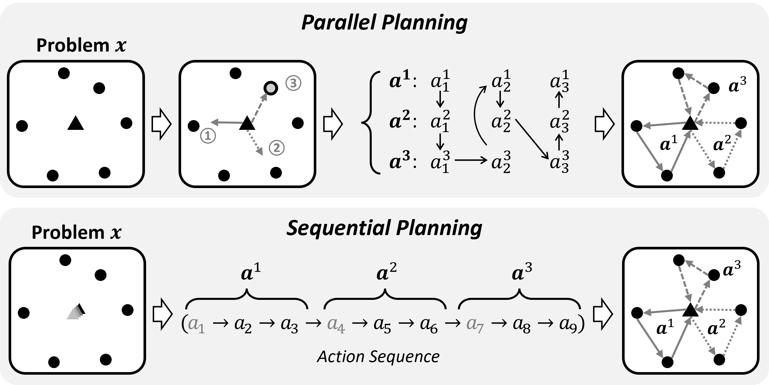
Figure 1: Illustration of parallel planning and sequential planning on min-max VRPs. In sequential planning, when an action selects a depot index (gray colored $a_{t}$), the planning for currently active agent is terminated to start planning for the new agent that corresponds to the selected depot.

Our method performs remarkably well at the min-max routing problems, outperforming both existing classical heuristic and learning-based methods. As a highlight, Equity-Transformer achieves 334$\times$ speed improvement and 53% reduction of solution cost compared to the representative classical heuristic solver (LKH3) when solving the multi-agent TSP with 1,000 cities. Also, our method achieves 1,217$\times$ faster speed and 9% reduction of solution cost than the representative learning-based method (ScheduleNet) with parallel planning.

Problem Formulation

In our work, we focus on tackling min-max routing problems, which involve a scenario where a group of $M$ agents needs to visit $N$ cities with the objective of minimizing the maximum tour length among the individual tours of the agents. In this section, we present the formulation of min-max routing through the lens of sequential planning.

Problem.

A routing problem is defined the set of city locations and a depot, represented as $\bm{x}=\{x_{i}\}_{i=1}^{N}$ where $x_{i}\in\mathbb{R}^{2}$ is the Cartesian coordinates, and $x_{1}$ denotes the depot. Since the $M$ agents find tours that start from the depot and return to the depot, we add $M$ dummy depot (each dummy depot assigned to each agent), i.e., $x_{N+1}=\cdots=x_{N+M}=x_{1}$. Thus, the sequential planning routing is defined as $\bm{x}=\{x_{i}\}_{i=1}^{N+M}$. Remarks that we can expand the definition of $\bm{x}$ so that it can include additional features required for other problems like the capacitated vehicle routing. For simplicity, we represent locations only.

Action.

The sequential planning is represented as an action sequence $\bm{a}=(a_{1},\ldots,a_{N+M})$. This action sequence is formed by selecting an index from the set of unvisited nodes at step $t$, i.e., $a_{t}\in\{1,\ldots,N+M\}\setminus\{a_{1},\ldots,a_{t-1}\}$. The resulting action sequence is partitioned into $M$ subsequences, i.e., agent tours $(\bm{a}^{1},\ldots,\bm{a}^{M})$, by splitting $\bm{a}$ with depot choosing actions. Thus, each $\bm{a}^{m}=(a^{m}_{1},\ldots,a^{m}_{L_{m}})$ starts with a dummy depot index, i.e., $a^{m}_{1}\in\{N+1,\ldots,N+M\}$, followed by subsequent city indices. Please refer to Figure 1.

State.

The state $s_{t}$ is defined as the union of the precollected actions $a_{1},\ldots,a_{t-1}$ and the problem $\bm{x}$, i.e., $s_{1}=\{\bm{x}\}$, and $s_{t}=\{a_{1},\ldots,a_{t-1};\bm{x}\}$ for $t>1$.

Cost.

The cost is the maximum tour length among all agents’ tours of $(\bm{a}^{1},\ldots,\bm{a}^{M})$ of given action sequence $\bm{a}$, i.e.,

$$\mathcal{L}_{\text{cost}}(\bm{a};\bm{x}):=\max\left\{\mathcal{L}(\bm{a}^{1};\bm{x}),...,\mathcal{L}(\bm{a}^{M};\bm{x})\right\},\mbox{where}$$

$$\mathcal{L}(\bm{a}^{m};\bm{x}):=\sum_{t=2}^{L_{m}}||x_{a^{m}_{t}}-x_{a^{m}_{t-1}}||_{2}+||x_{a^{m}_{1}}-x_{a^{m}_{L_{m}}}||_{2}.$$

Policy.

The policy $\pi_{\theta}(\bm{a}|\bm{x})$ is a composition of segment policy $\pi_{\theta}(a_{t}|\bm{s}_{t})$, generating action sequences for given problem condition $\bm{x}$ according to the following expression.

$$\pi_{\theta}(\bm{a}|\bm{x})=\prod_{t=1}^{N+M}\pi_{\theta}(a_{t}|\bm{s}_{t}).$$

The $\theta$ is the deep neural network parameter of the policy $\pi$. The optimal parameter $\theta^{*}$ can be determined by solving the following optimization problem:

$$\theta^{*}=\operatorname*{arg\,min}_{\theta}\mathbb{E}_{P(\bm{x})}\mathbb{E}_{\pi_{\theta}(\bm{a}|\bm{x})}\mathcal{L}_{\text{cost}}(\bm{a};\bm{x}),$$

where $P(\bm{x})$ is the distribution of problem $\bm{x}$.

Methodology

This section presents the architecture of Equity-Transformer $\pi_{\theta}(\bm{a}|\bm{x})$, which generates an action sequence $\bm{a}=(a_{1},\ldots,a_{N+M})$ for a given problem $\bm{x}$. Our high-level idea is to build a transformer model with multi-agent positional encoding and equity context.

Our architecture has the following forward propagation:

1. Multi-agent positional encoding for initial node embedding given problem $\bm{x}$.

2. Employ the encoder of Transformer (Vaswani et al. 2017) to the initial node embedding to obtain $\bm{H}=[h_{1},\ldots,h_{N+M}]\in\mathbb{R}^{D\times(N+M)}$, where $D$ is the embedding dimension.

3. Iterative decoding $t=1,\ldots,N+M$ using

   1. Equity context encoding for $\bm{c}_{t}\in\mathbb{R}^{D}$.

   2. Decoding to produce $\bm{a}_{t}\sim\pi_{\theta}(\bm{a}_{t}|\bm{H},\bm{c}_{t})$ by using $c_{t}$ as attention query of decoder.

The encoding and the iterative decoding procedure process involving contextual queries have been comprehensively addressed in the previous literature (Kool, van Hoof, and Welling 2019; Kwon et al. 2020; Li et al. 2021; Kim, Park, and Park 2022). In this paper, we focus on introducing new elements designed for min-max routing problems, which are multi-agent positional encoding and equity context encoding.

Multi-agent Positional Encoding

We begin with partitioning the problem $\bm{x}$ into two distinct components: the cities, denoted as $\bm{x}_{\text{city}}$ with elements $\{x_{i}\}_{i=1}^{N}$, and the agents, represented by $\bm{x}_{\text{agent}}$ with elements $\{x_{i}\}_{i=N+1}^{N+M}$. In order to facilitate sequential relationships between the agents, we employ positional encoding $f_{\text{PE}}$ to $\bm{x}_{\text{agent}}$. This positional encoding incorporates sine and cosine functions with differing frequencies, following the work by Vaswani et al. (2017).

Next, we concatenate the linearly projected vectors of $\bm{x}_{\text{city}}$ and $f_{\text{PE}}(\bm{x}_{\text{agent}})$ to form the initial node embedding. The embedding is subsequently fed into the encoder, a structural component akin to the encoder of AM as illustrated in Figure 2. It is worth to note that the original AM architecture itself is not appropriate for addressing multi-agent problems, due to its incapability to consider the multi-agent nature. In contrast, our approach incorporates positional encoding to $\bm{x}_{\text{agent}}$ with the specific intention of introducing a virtual order bias. Consequently, we can sequentially generate the tour sequence of an agent while considering both preceding and succeeding agents in the assigned order.

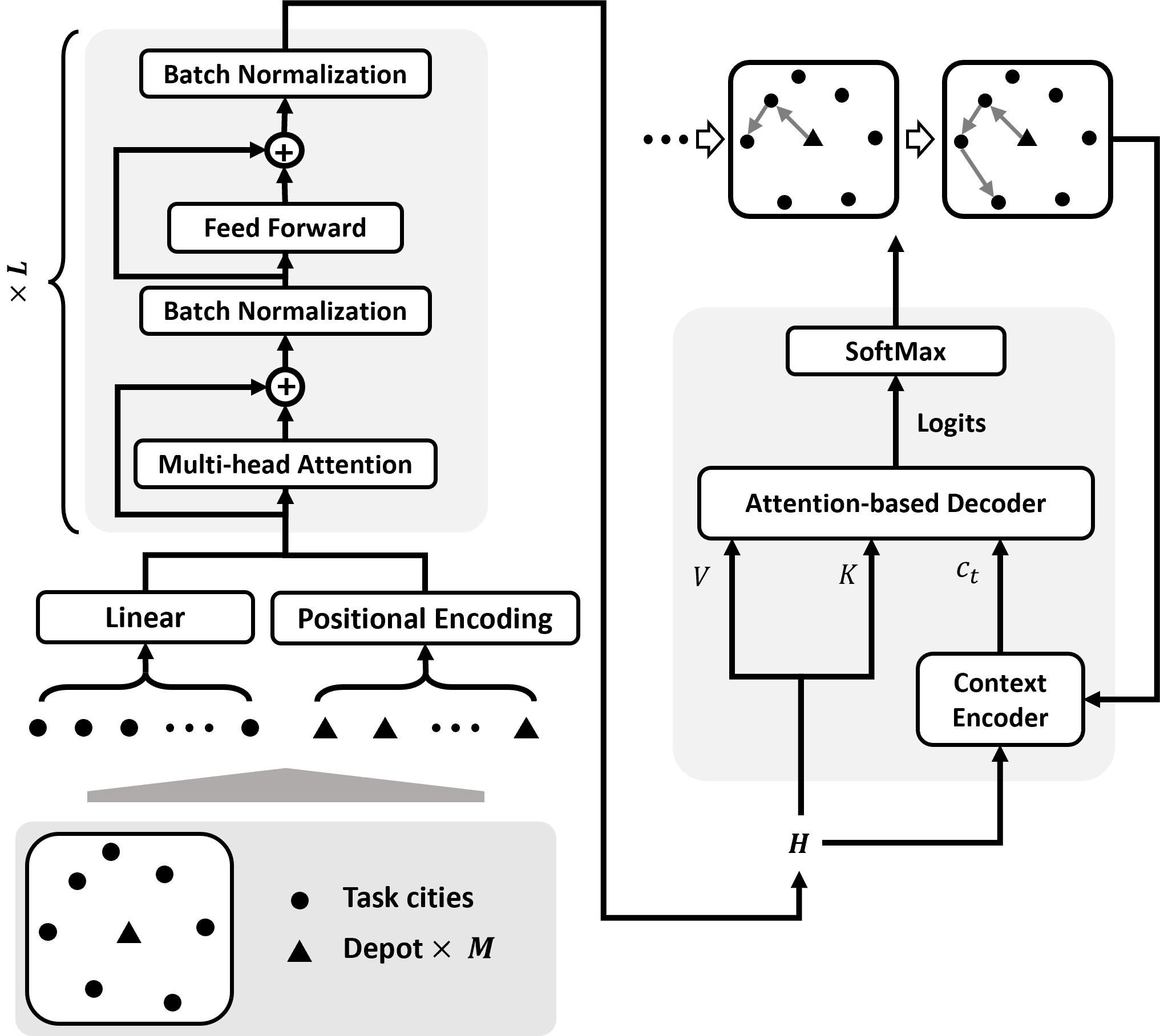
Figure 2: Illustration of Equity-Transformer. The $L$ stands for the number of sequential layers, where we set $L=3$.

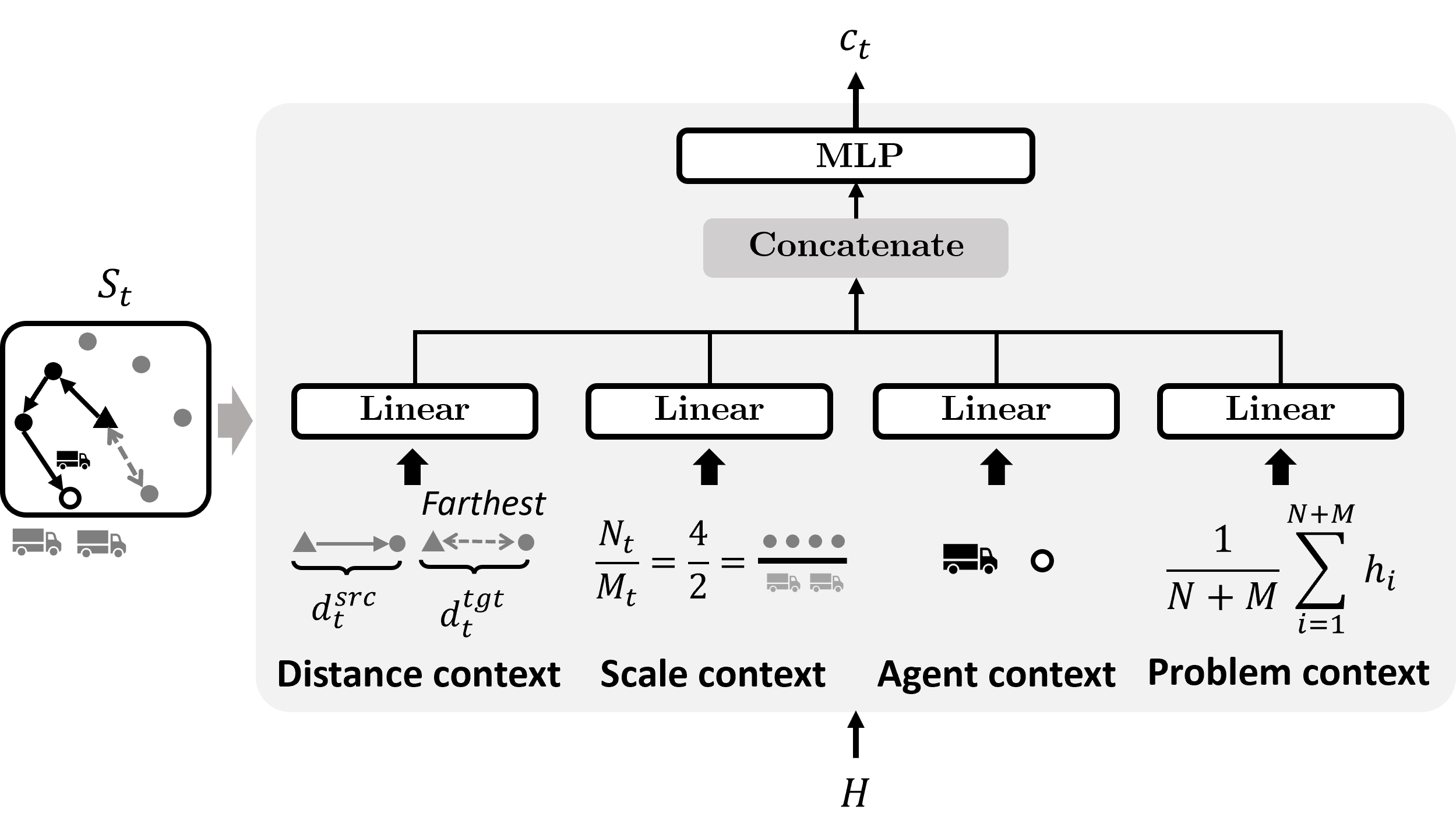
Figure 3: Illustration of equity context encoding

Equity Context Encoding

For every decoding step $t$, we utilize four distinct contexts as ingredients of the equity context, $\bm{c}_{t}$. Each of the ingredient contains useful information for equitable decoding, described as follows:

• Problem context $\bm{h}^{\text{problem}}\in\mathbb{R}^{D}$: The problem context collects the average of representations
  $\bm{h}^{\text{problem}}=\frac{1}{M+N}\sum_{i=1}^{M+N}\bm{h}_{i}$. This aligns with the context embedding of AM, which is primarily intended to capture the global context of problem $\bm{x}$ by averaging each city and agent representation.

• Agent context $\bm{h}^{\text{agent}}_{t}\in\mathbb{R}^{D}$: We set agent context using representations of the returning depot and the last visited city of the current active agent $m_{t}$. Precisely, $\bm{h}^{\text{agent}}_{t}=g_{\text{agent}}(\bm{h}_{N+m_{t}}\oplus\bm{h}_{a_{t-1}})$, where $g_{\text{agent}}:\mathbb{R}^{2D}\rightarrow\mathbb{R}^{D}$ represents a linear projection. This context highlights the currently active agents.

• Scale context $\bm{h}^{\text{scale}}_{t}\in\mathbb{R}^{D}$: We incorporate the ratio between $N_{t}$ and $M_{t}$ as a scaling context, where $N_{t}$ represents the number of remaining cities and $M_{t}$ denotes the current number of un-used agents at the depot, i.e., $N_{t}/M_{t}\in\mathbb{R}$. We then generate $\bm{h}^{\text{scale}}_{t}=g_{\text{scale}}\left(N_{t}/M_{t}\right)$, where $g_{\text{scale}}:\mathbb{R}\rightarrow\mathbb{R}^{D}$ represents a linear projection. This context offers valuable insights into the approximate number of cities an agent should visit to achieve equity. Consequently, the scale ratio can provide the effective information to decide whether to continue visiting additional cities or return to the depot.

• Distance context $\bm{h}^{\text{dist}}_{t}\in\mathbb{R}^{D}$: We make use of dynamic changes in the agent’s tour length and the distance of remaining cities from the depot at the current step $t$. Firstly, we employ $d_{t}^{\text{source}}$, which represents the current tour length of the active agent. Secondly, we utilize $d_{t}^{\text{target}}$, which denotes the maximum distance between the depot and the remaining unvisited cities. Subsequently, we form $\bm{h}^{\text{dist}}_{t}=g_{\text{dist}}(d_{t}^{\text{source}}\oplus d_{t}^{\text{target}})$, where $g_{\text{dist}}:\mathbb{R}^{2}\rightarrow\mathbb{R}^{D}$ is a linear projection. This information holds significant importance in terms of the equity of tour length among agents in the min-max routing problem. The context prompts the decoders to consider the agent’s current tour length and remaining tasks, aiding in the decision-making process of whether to stop visiting (i.e., return to the depot) or continue the tour while considering the min-max tour length.

The context encoder $f_{\text{CE}}:\mathbb{R}^{4D}\rightarrow\mathbb{R}^{D}$, which is a multi-layer perception (MLP), produces equity context $\bm{c}_{t}$ using these four contexts, i.e.,

$$\bm{c}_{t}=f_{\text{CE}}(\bm{h}^{\text{problem}}\oplus\bm{h}^{\text{agent}}_{t}\oplus\bm{h}^{\text{scale}}_{t}\oplus\bm{h}^{\text{dist}}_{t}).$$

We adopt an approach similar to that of Kool, van Hoof, and Welling (2019), where use $\bm{c}_{t}$ as a contextual query for the attention-based decoder $\pi_{\theta}(\bm{a}_{t}|\bm{H},\bm{c}_{t})$, as shown in Figure 3. This utilization of task-equity information from the equity context enables the decoder to sequentially generate balanced tours.

Training Scheme

The Equity-Transformer is trained with REINFORCE (Williams 1992) with the shared baseline scheme similar to Kwon et al. (2020) and Kim, Park, and Park (2022). The shared baseline with symmetric samples makes symmetric exploration for the combinatorial solution space. The training loss with the symmetric shared baselines is as follows:

$$\begin{split}\mathcal{L}_{\text{train}}(\bm{\theta})&=\mathbb{E}_{P(\bm{x})}\mathbb{E}_{\pi_{\theta}(\bm{a}|\bm{x})}\mathcal{L}_{\text{cost}}(\bm{a};\bm{x}),\\ \nabla\mathcal{L}_{\text{train}}(\bm{\theta})&\approx\sum_{i=1}^{B}\sum_{j=1}^{L}\left(\mathcal{L}_{\text{cost}}\left(\bm{a}^{(i,j)};\bm{x}^{(i)}\right)-b_{\text{shared}}\right),\end{split}$$

where $b_{\text{shared}}:=1/L\sum_{j=1}^{L}\mathcal{L}_{\text{cost}}(\bm{a}^{(i,j)};\bm{x}^{(i)})$. Each $\bm{a}^{(i,l)}$ is sampled sequence from training solver given $L$ symmetric $\bm{x}^{(i)}$: $\pi_{\theta}(\bm{a}|\mathcal{T}_{1}(\bm{x}^{(i)})),...,\pi_{\theta}(\bm{a}|\mathcal{T}_{L}(\bm{x}^{(i)}))$, where $\mathcal{T}_{1},...,\mathcal{T}_{L}$ are symmetric transformation of problem instance $\bm{x}^{(i)}$. See Kim, Park, and Park (2022) for a detailed training scheme.

Experiments

		Classic-based				Learning-based
$N$	$M$	LKH3 (60)	LKH3 (600)	OR-Tools (60)	OR-Tools (600)	SN	NCE	ET (ours)
200	10	2.52 (60)	2.08 (600)	4.97 (60)	2.22 (600)	2.35 (9.70)	2.07 (5.07)	2.05 (0.36)
	15	2.39 (60)	2.03 (600)	4.82 (60)	2.15 (600)	2.13 (10.52)	1.97 (5.07)	1.97 (0.37)
	20	2.29 (60)	2.02 (600)	3.74 (60)	2.04 (600)	2.07 (11.40)	1.96 (5.07)	1.96 (0.37)
500	30	3.31 (60)	2.70 (600)	7.90 (60)	6.44 (600)	2.16 (171)	2.07 (5.20)	2.02 (0.87)
	40	3.10 (60)	2.55 (600)	7.46 (60)	6.69 (600)	2.12 (276)	2.01 (5.38)	2.01 (0.90)
	50	2.93 (60)	2.48 (600)	8.50 (60)	7.26 (600)	2.09 (217)	2.01 (5.05)	2.01 (0.92)
1000	50	4.45 (60)	3.77 (600)	11.65 (60)	9.89 (600)	2.26 (2094)	2.13 (15.05)	2.06 (1.72)
	75	3.71 (60)	3.26 (600)	13.16 (60)	11.50 (600)	2.17 (1678)	2.07 (15.05)	2.05 (1.80)
	100	3.23 (60)	2.92 (600)	10.79 (60)	8.93 (600)	2.16 (1588)	2.05 (15.01)	2.05 (1.79)
2000	100	6.60 (60)	4.61 (600)	20.99 (60)	18.85 (600)	OB	2.85 (43.96)	2.09 (3.49)
	150	5.08 (60)	4.02 (600)	14.00 (60)	13.17 (600)	OB	2.83 (44.77)	2.08 (3.41)
	200	4.13 (60)	3.36 (600)	11.00 (60)	10.41 (600)	OB	2.08 (30.30)	2.08 (3.60)
5000	300	12.30 (60)	7.87 (600)	17.00 (60)	17.00 (60)	OB	2.97 (290)	2.40 (8.78)
	400	8.85 (60)	6.15 (600)	13.00 (60)	13.00 (600)	OB	2.92 (204)	2.21 (8.61)
	500	7.14 (60)	5.37 (600)	11.00 (60)	11.00 (600)	OB	2.89 (198)	2.19 (9.02)

Table 1: Results on min-max mTSP. Every performance is average performance among 100 instances. The bold symbol indicates the best performance. Average running times (in seconds) are provided in brackets.

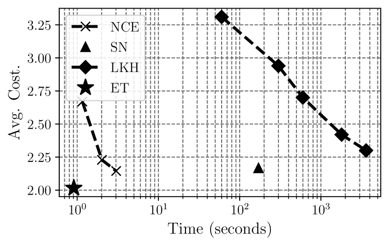
(a) mTSP with $(500,30)$

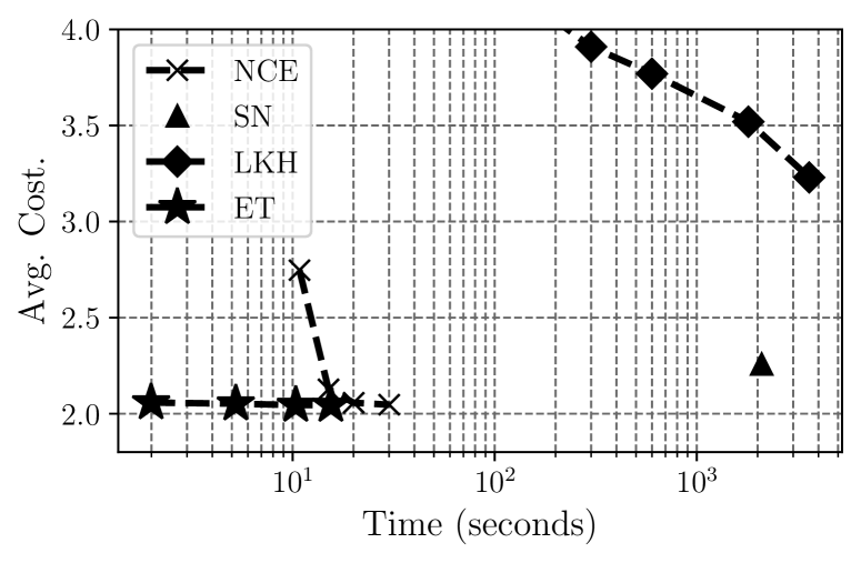
(b) mTSP with $(1000,50)$

Figure 4: Time-performance trade-off graph for mTSP. The left and bottom indicate the Pareto frontier.

In this section, we present the experimental results of the Equity-Transformer model on two min-max routing problems: the multi-agent traveling salesman problem (mTSP) and the multi-agent pick-up and delivery problem (mPDP).

Training Setting.

we use uniform distribution for the problem distribution $P(\bm{x})$, following Kool, van Hoof, and Welling (2019). For the training hyperparameters we set exactly the same hyperparameters for every task and experiment; see Appendix B. We train Equity-Transformer on $N=50$, and finetune it to target distribution of $N=200,500$. The training time for the min-max mTSP is approximately one day, while for the min-max mPDP, it takes around four days.

Experiments Metric.

It is important to carefully measure the performance comparison between methods, as often there is a trade-off between run time and solution quality. To this end, we present time-performance multi-objective graphs to compare tradeoffs between performance and computation time. In the result tables, we present the average cost achieved within a specific time limit, recognizing that every method has the potential to reach optimality given an unlimited amount of time.

Target Problem Instances.

To evaluate the performance of our methods, we report results on randomly generated synthetic instances of min-max mTSP and min-max mPDP at different problem scales of $N$ and $M$. We generate the 100 problems set with a uniform distribution of node locations per scale. We conduct experiments with $N=200,500,1000,2000,5000$ and set $M$ such that $10\leq N/M\leq 20$ by referring practical setting of min-max routing application (Ma et al. 2021).

Speed Evaluation.

All experiments were performed using a single NVIDIA A100 GPU and an AMD EPYC 7542 32-core processor as the CPU. Comparing the speed performance of classical algorithms (CPU-oriented) and learning algorithms (GPU-oriented) poses a significant challenge (Kool, van Hoof, and Welling 2019; Kim, Park, and Kim 2021), given the need for a fair evaluation. While certain approaches exploit the parallelizability of learning algorithms on GPUs, enabling faster solutions to multiple problems than classical algorithms, our method follows a serial approach in line with the prior min-max learning methods (Park, Kwon, and Park 2023; Kim, Park, and Park 2023). Note that when we leverage the parallelizability of our method, our approach can achieve speeds more than $100\times$ faster; refer to Appendix A.

Performance Evaluation on mTSP

Baselines for mTSP.

We consider two representative deep learning-based baseline algorithms: the ScheduleNet (Park, Kwon, and Park 2023) and Neuro Cross Exchange (Kim, Park, and Park 2023) for min-max mTSP. For conciseness, We denote them as SN and NCE respectively. We have also included two classical heuristic methods, namely LKH3 (Helsgaun 2017) and OR-Tools (Perron and Furnon 2019), with respective time limits of 60 seconds and 600 seconds per instance. Specifically, LKH3 utilizes $\lambda$-opt improvement iterations to enhance the solution within the given time budget. The time limit directly influences the number of iterations performed (following the approach in Xin et al. (2021b)). Similarly, OR-Tools incorporates an iterative local search procedure for solution improvement, with the time limit governing the iterations of the local search.

Results.

The results in Table 1. demonstrate that the Equity-Transformer (denoted as ‘ET’ in tables and figures) outperforms all baselines with impressive speed. As the problem scale increases, the performance gap between ET and other methods widens further. Specifically, for $N=1000$ and $M=100$, ours achieves a cost of 2.05, significantly better than LKH3 (2.92) and NCE (2.16). Moreover, our method is $15.01/1.79\approx 8.39\times$ faster than NCE and about $600/1.79\approx 335\times$ faster than LKH3. The time-performance trade-off analysis shown in Fig. 4 confirms that our method outperforms every baseline and provides the Pareto frontier on multi-objective of time and cost.

For the large-scale problem of $N=5000$, the ScheduleNet suffers from the complexity inherent in the parallel planning, failing to produce a solution within 10,000 seconds per problem, making it out-of-budget ($OB$). While LKH3 and OR-Tools methods can provide solutions within the allotted time, their performance is inadequate due to the inherent difficulty of large-scale problems, requiring a significantly higher number of improvement iterations for low-cost solutions. On the other hand, the NCE method surpasses classical approaches, as claimed in their main paper, but our method outperforms NCE by a substantial margin of approximately $290/8.78\approx 33\times$ faster speed and $(2.97-2.40)/2.97\approx 19\%$ reduced cost.

Performance Evaluation on mPDP

		Classic-based		Learning-based
$N$	$M$	OR-Tools (60)	OR-Tools (600)	AM	AM†	HAM	HAM†	ET (ours)	ET† (ours)
200	10	20.96 (60)	18.76 (600)	15.88 (0.33)	15.65 (0.67)	5.69 (0.33)	5.30 (0.55)	5.03 (0.54)	4.68 (0.55)
	15	13.96 (60)	8.46 (600)	15.88 (0.33)	15.57 (0.69)	5.21 (0.34)	5.09 (0.57)	3.91 (0.55)	3.65 (0.56)
	20	10.67 (60)	5.70 (600)	15.88 (0.35)	15.55 (0.71)	5.21 (0.35)	5.09 (0.61)	3.39 (0.56)	3.18 (0.61)
500	30	16.99 (60)	16.99 (600)	26.98 (0.82)	26.15 (3.10)	9.10 (0.84)	8.86 (1.92)	4.38 (1.33)	4.11 (1.55)
	40	12.99 (60)	12.65 (600)	26.98 (0.86)	26.14 (3.17)	9.10 (0.84)	8.87 (1.95)	3.75 (1.36)	3.52 (1.62)
	50	10.99 (60)	10.41 (600)	26.98 (0.85)	26.14 (3.20)	9.10 (0.88)	8.87 (1.95)	3.44 (1.38)	3.23 (1.66)
1000	50	21.00 (60)	21.00 (600)	40.86 (1.61)	39.63 (11.28)	15.12 (1.63)	14.58 (6.35)	4.91 (2.63)	4.73 (3.56)
	75	14.00 (60)	14.00 (600)	40.86 (1.68)	39.61 (11.44)	15.12 (1.70)	14.59 (6.41)	3.96 (2.65)	3.77 (3.63)
	100	11.00 (60)	10.98 (600)	40.86 (1.69)	39.63 (11.24)	15.12 (1.72)	14.61 (6.61)	3.56 (2.75)	3.38 (3.80)
2000	100	21.00 (60)	21.00 (600)	62.85 (3.24)	61.31 (24.98)	25.68 (3.40)	25.06 (15.17)	5.15 (5.22)	4.91 (9.22)
	150	14.00 (60)	14.00 (600)	62.85 (3.34)	61.28 (25.43)	25.68 (3.40)	25.04 (16.26)	4.17 (5.31)	3.97 (9.50)
	200	11.00 (60)	11.00 (600)	62.85 (3.35)	61.33 (26.33)	25.68 (3.50)	25.06 (16.47)	3.79 (5.43)	3.62 (10.01)
5000	300	17.00 (60)	17.00 (600)	114.73 (8.30)	112.84 (180)	54.07 (34.65)	53.46 (279)	4.81 (52.66)	4.60 (79.23)
	400	13.00 (60)	13.00 (600)	114.73 (8.31)	112.90 (182)	54.07 (34.44)	53.43 (283)	4.33 (54.86)	4.11 (82.59)
	500	11.00 (60)	11.00 (600)	114.73 (8.33)	112.83 (186)	54.07 (34.46)	53.45 (286)	4.12 (54.77)	3.88 (82.87)

Table 2: Results on min-max mPDP. Every performance is average performance among 100 instances. The bold symbol indicates the best performance. Average running times (in seconds) are provided in brackets.

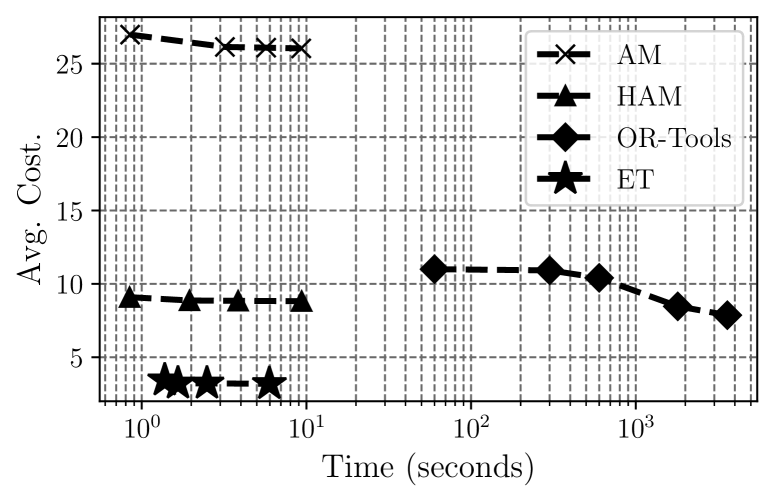
(a) mPDP with $(500,50)$

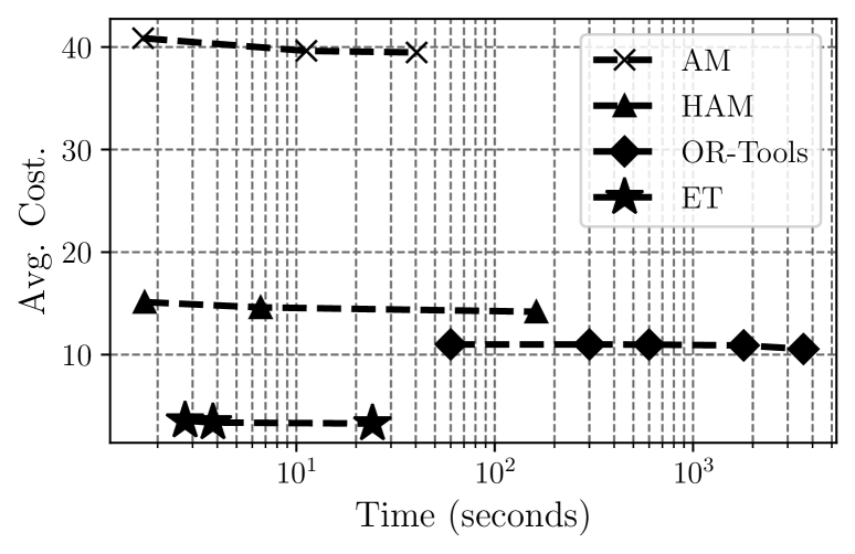
(b) mPDP with $(1000,100)$

Figure 5: Time-performance trade-off graph for mPDP. The left and bottom indicate the Pareto frontier.

Baselines for mPDP.

We consider representative two deep learning-based baseline algorithms: AM (Kool, van Hoof, and Welling 2019) and heterogeneous AM (Li et al. 2021), denoted as HAM. We retrain AM, and HAM using min-max objective; the details are provided in Appendix B. We also marked $\dagger$ by giving more trials for inference solutions such as sampling width (Kool, van Hoof, and Welling 2019) and augmentation width (Kwon et al. 2020); see Appendix B for the details. We also include a heuristic method, OR-Tools (Perron and Furnon 2019), while LKH3 (Helsgaun 2017) cannot handle min-max mPDP to the best of our knowledge. We exclude the multi-agent PDP (MAPDP) model (Zong et al. 2022) due to the inaccessible source code.

The results presented in Table 2 demonstrate that our methods (i.e., ET and ET^†) outperform all other baselines, aligning with the findings from the mTSP experiments. Compared to OR-Tools, ET^† exhibits a remarkable speed improvement of $600/0.55\approx 1901\times$, while reducing the objective cost by approximately $(18.76-4.68)/18.76\approx 75\%$ at $N=200,M=10$. Moreover, as shown in Figure 5, our method consistently presents the Pareto frontier compared to other baselines.

Importantly, in certain instances, both AM and HAM produce identical cost values as the number of agents $M$ increases. For instance, when $N=500$, AM and HAM yield the same scores for $M=30,40,50$. These methods were primarily designed to address min-sum problems (with HAM especially focusing on min-sum mPDP), exhibiting a limited emphasis on leveraging the concept of equity among agents. These findings serve as compelling evidence supporting the success of our design choice centered around equity considerations.

Ablation Study

To assess the influence of each component within our methodology on performance enhancement, we conducted an ablation study. As illustrated in Table 3, both components of our approach yielded significant performance improvements. Notably, the $\emptyset$ configuration, which represents the absence of these components, resulted in the poorest performance, indicating that a straightforward application of sequential planning to the min-max routing problem is not inherently promising. However, when we combined the multi-agent positional encoder (MPE) and the context encoder (CE), we observed substantial performance improvements, particularly in larger-scale scenarios.

$N$	100			200
$M$	5	10	15	10	15	20
$\emptyset$	2.86	2.12	2.12	2.92	2.90	2.90
$\{\text{MPE}\}$	2.35	1.97	1.96	2.51	2.33	2.80
$\{\text{CE}\}$	2.52	1.97	1.95	2.28	2.01	1.98
$\{\text{MPE},\text{CE}\}$	2.35	1.96	1.95	2.15	1.99	1.98

Table 3: Ablation study for the combination of Equity-Transformer components. The $\emptyset$ represents the AM without our components. The MPE and CE stand for the multi-agent positional encoding and context encoder.

Ablation Study for Order Bias.

As depicted in Figure 6, MPE contributes to inducing an order bias among agents by generating cyclic sub-tours in the Euclidean space with specific orders. This can be interpreted as successful modeling of tour generation in the Euclidean space from multiple agents in the sequence space, which is the primary objective of MPE.

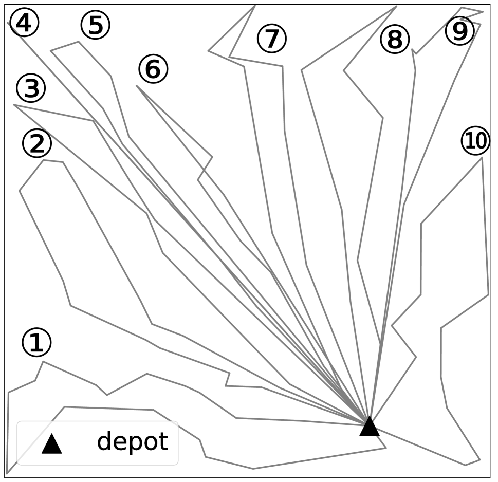
(a) With MPE

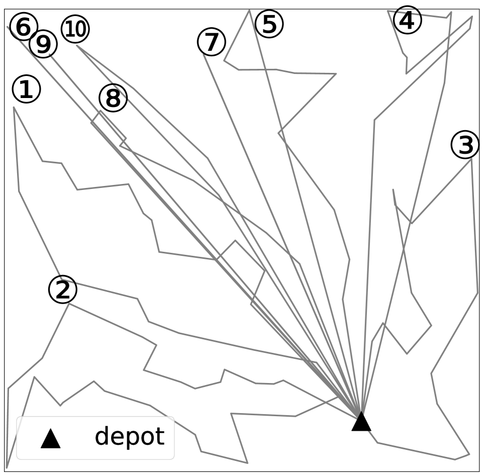
(b) Without MPE

Figure 6: Ablation study for the multi-agent positional encoding (MPE) on mTSP with $N=100$ and $M=10$.

Additional Experiments

We conducted several additional experiments in the Appendix C and Appendix D. First, we validate the performance of the Equity-Transformer in a real-world benchmark dataset (Appendix C). Among the baseline methods, Equity-Transformer demonstrates superior performance in almost all instances. Moreover, we assessed the robustness of Equity-Transformer under various problem distributions (Appendix D.1) and different $N/M$ ratios (Appendix D.2), comparing it with LKH3. These experiments confirmed the robustness of Equity-Transformer to the changes in problem distributions and $N/M$ ratios. Lastly, we compared Equity-Transformer with two competitive two-stage mTSP solvers (Hu, Yao, and Lee 2020; Liang et al. 2023), and ours outperformed them in terms of performance (Appendix D.3).

Related Work

Vehicle Routing Problems

After Vinyals, Fortunato, and Jaitly (2015) suggested the Pointer Networks, which constructively generate permutation sequences as routing solutions, termed constructive solver, Bello et al. (2017) turns it into deep reinforcement learning. Kool, van Hoof, and Welling (2019) reinvent the Pointer Network using a transformer, termed attention model (AM), which becomes standard architecture for solving vehicle routing problems. By extending AM into various applications, including those outlined in recent research (Li et al. 2021; Jiang et al. 2022; Ma et al. 2021; Xin et al. 2021a; Ma et al. 2021, 2022), several challenges within the field of vehicle routing are addressed. In recent studies, there has been a notable emphasis on assessing the robustness of neural solvers concerning both scale shift (Hottung, Kwon, and Tierney 2021; Son et al. 2023) and distributional shift (Jiang et al. 2022; Bi et al. 2022; Zhou et al. 2023).

Independent of constructive solution generation, other studies try to solve VRPs by learning to iteratively revise the solution, terms improvement solver. Chen and Tian (2019); Li, Yan, and Wu (2021); Kim, Park, and Kim (2021); Wang et al. (2021) leverages local solver to rewrite partial tour to improve solution. Some studies train existing local search solvers such as 2-opt heuristic (da Costa et al. 2020; Wu et al. 2021), large neighborhood search (Hottung and Tierney 2020), iterative dynamic programming (Kool et al. 2021), and LKH (Xin et al. 2021b) using deep learning. Some studies use fine-tuning schemes focused on test-time adaptation in iterative learning (Hottung, Kwon, and Tierney 2021; Choo et al. 2022). While a constructive solver is invaluable for quickly generating an initial feasible solution, an improvement solver plays a crucial role in refining the solution to achieve enhanced optimality. These two approaches are fundamentally distinct and orthogonal in their objectives.

Min-Max Vehicle Routing Problems

Most deep learning-based VRPs studied focus on min-sum routing which focuses on minimizing total tour length among multiple agents. The min-max routing problem focuses on minimizing the maximum tour length among multiple agents, making it highly relevant for time-critical tasks such as disaster management and vaccine delivery. The min-max routing method considers the equity of tours among the multiple agents (França et al. 1995).

In constructive approaches, Cao, Sun, and Sartoretti (2021) and Park, Kwon, and Park (2023) advocate for a constructive solver that models decentralized parallel decisions made by multiple agents. Additionally, in addressing the specific challenge of min-max mTSP with time windows and rejections, Zhang et al. (2022) introduce a constructive solver leveraging a graph neural network in conjunction with meticulous training and inference strategies.

On the other hand, in the domain of improvement-based methodologies, Kim, Park, and Park (2023) propose an enhancement solver that learns to optimize tour components through cross-exchanges. Meanwhile, Hu, Yao, and Lee (2020) and Liang et al. (2023) advocate a two-stage solver approach, wherein the initial stage employs a constructive solver, followed by an improvement solver tasked with refining the solution further.

Conclusion

This paper introduced Equity-Transformer, sequential models for min-max routing problems. Our method outperformed the existing classic methods and state-of-the-art neural solvers, achieving a Pareto frontier in balancing cost and runtime on representative tasks like mTSP and mPDP. Our method demonstrates its scalability, handling large-scale cities with up to $N=5000$ nodes and agent fleets of up to $M=500$. Equity-Transformer holds potential for broader applications in general min-max vehicle routing problems, which we identify as a promising avenue for future research.

Appendix A Speed Evaluation for Serial and Parallel Process

This section provides an evaluation of the speed performance of Equity-Transformer in two distinct scenarios: the serial process, where instances are solved one by one in a sequential manner, and the parallel process, where instances are solved concurrently. The results, illustrated in Table 4, clearly demonstrate that Equity-Transformer exhibits remarkable parallelization capabilities, resulting in a speed improvement of approximately 153 times compared to the serial process for the mTSP with 500 instances and $N=1000$. This significant enhancement underscores the potential of Equity-Transformer to efficiently handle multiple routing problem requests simultaneously in real-world situations. It is worth noting that even in the serial process, as shown in the main table, Equity-Transformer surpasses the baseline method in terms of speed, without leveraging any parallelization advantages.

$N$	Number of instances	Serial Process	Parallel Process
200	10	3.30s	1.36s
	100	33.67s	1.51s
	500	169.55s	2.98s
500	10	8.37s	1.93s
	100	84.13s	2.84s
	500	449.05s	3.68s
1000	10	16.48s	3.02s
	100	163.75s	4.53s
	500	815.52s	5.35s

Table 4: Comparison of total time for solving instances in mTSP with the serial process and parallel process in Equity-Transformer. The s stands for the seconds.

Appendix B Detail of Experimental Setting

B.1 Datasets

In the mTSP experiment, we generate a random mTSP instance by randomly selecting $N$ nodes from the unit square. As per convention, we designate the depot as the first index among the $N$ nodes. Similarly, in the mPDP experiment, we generate the locations of the depot and customer nodes (pickup and delivery pairs) randomly and independently. Note that the first half of the customer nodes are assigned as pickup nodes, while the second half serves as delivery nodes.

B.2 Equity-Transformer

During the training step of Equity-Transformer (ET), we adopt the same hyperparameters as described in (Kool, van Hoof, and Welling 2019). In the finetuning step, we specifically focus on adjusting the $\theta_{\text{context}}$ parameter with $N=200,500$ for mTSP and $N=200$ for mPDP. For inference instances, we employ the finetuned model with $N=200$ for mTSP $N=200$, $N=500$ for mTSP $N>500$, and $N=200$ for mPDP. Additionally, we incorporate an augmentation technique following the methodology outlined in Kwon et al. (2020). Finally, ET^† incorporates a sampling strategy where 100 samples are taken for each instance, and the best result among those samples represents the performance of ET^†.

	Hyperparameters	mTSP	mPDP
Training	Learning rate	1e-4	1e-4
	Batch-size	512	512
	Epochs	100	100
	Epoch size	1,280,000	1,280,000
Finetuning	Learning rate	1e-5	1e-5
	Batch-size	128	128
	Finetuning-time	15h	15h
Inference	Augmentation	8	8

Table 5: Hyperparameter setting for Equity-Transformer in mTSP and mPDP.

B.3 LKH3

LKH3 (Helsgaun 2017) is an extension of the Lin-Kernighan algorithm, an effective local-search heuristic for addressing TSP. LKH3 exhibits the capability to tackle not only TSP but also a diverse range of constrained routing problems, by minimizing a penalty function that quantifies the degree of a constraint violation. However, LKH3 does not support solving algorithms for the mPDP, limiting its application to the mTSP in our work. We use the executable program of LKH3, which is publicly available.

Name	Value
Max trials	1000
Runs	1
Seed	3333
Time limit	{60, 300, 600, 1800, 3600}

Table 6: Parameter setting for LKH3. It is worth noting that while we set specific values for the max trials and the runs, the algorithm predominantly terminated based on the time limit condition, especially when solving large scale problems. For the remaining parameters not mentioned, we use the default values provided by the program.

B.4 OR-Tools

OR-tools (Perron and Furnon 2019) is an open-source software that aims to solve various combinatorial optimization problems. OR-tools offers a wide range of solvers for tackling problems such as linear programming, mixed-integer programming, constraint programming, routing problems, and scheduling. Within the realm of routing problems, OR-Tools can easily handle both mTSP and mPDP by simply incorporating additional constraints tailored to each problem. The installation guide for python OR-tools library and example codes for various problems, including mTSP and mPDP, are readily available in their official website.

Name	Value
Global span cost coefficient	10000
First solution strategy	PATH_CHEAPEST_ARC
Local search metaheuristic	GUIDED_LOCAL_SEARCH
Time limit	{60, 300, 600, 1800, 3600}

Table 7: Parameter setting for OR-tools. We use the same parameters for both mTSP and mPDP. Note that the global span cost coefficient should be sufficiently large to guarantee the desired objective for the min-max tasks. For the remaining parameters not mentioned, we use the default values suggested by OR-tools’ official guides.

B.5 ScheduleNet

ScheduleNet (SN) (Park, Kwon, and Park 2023) is a method that utilizes a graph neural network (GNN) to sequentially generate simultaneous actions for multiple agents, effectively capturing the relationships between them. To conduct our experiment, we obtained the source code by contacting the author and followed the training procedure outlined in (Park, Kwon, and Park 2023).

Name	Value
Learning rate	1e-4
Batch-size	512
Epochs	10,000
Epoch size	65,536
Discounting factor	0.9
Smoothing coefficient	0.1
Clipping parameter	0.2

Table 8: Hyperparameter for training ScheduleNet in mTSP.

B.6 Neuro Cross Exchange

The Neuro Cross Exchange (NCE) (Kim, Park, and Park 2023) is a supervised-learning-based improvement solver and a neural meta-heuristic technique that addresses vehicle routing problems (VRPs) by strategically swapping sub-tours among the vehicles to enhance solutions. We train a cost-decrement prediction model ($f_{\theta}(\cdot)$) using a number of cities ($N_{c}$) sampled from a uniform distribution $U(50,100)$. The number of depots ($N_{d}$) is set to 1, and the number of vehicles ($N_{v}$) is 2. The 2D coordinates of the cities are sampled from $U(0,1)$. With $N_{v}=2$, we generate two tours using the greedy assignment heuristic. From these two tours ($\tau_{1}$, $\tau_{2}$), we compute the best true cost-decrements for all feasible combinations to create the training dataset. Overall, we generated 47,856,986 training samples from 50,000 instances. The model $f_{\theta}(\cdot)$ is parameterized using a Graph Neural Network (GNN) with five layers of the attentive embedding layer. Additionally, we employ four-layered Multi-Layer Perceptrons (MLPs) to parameterize $\phi_{e}$, $\phi_{w}$, $\phi_{n}$, and $\phi_{c}$, with hidden dimensions of 64 and the Mish activation function.

We obtained the source code directly from the author by email. And we restrict the time because the improvement method will get the optimal solution when it has enough time. Table 9 describes the time limits we set for each problem size.

Number of cities ($N$)	Time limit
200	5.00
500	5.00
1,000	15.00
2,000	30.00
5,000	180.00

Table 9: Time limit for NCE in mTSP.

B.7 Attention Model

The Attention Model (AM) (Kool, van Hoof, and Welling 2019) serves as a fundamental component in numerous models, employing attention mechanisms to address a wide range of routing problems, including TSP, CVRP, PDP, and others. During the training phase, we adhere to the recommended hyperparameters provided by the open-source code. Additionally, we adopt a similar strategy for fine-tuning as ET. During the inference step, AM^† also utilizes the same strategy as ET^†.

	Name	Value
Training	Learning rate	1e-4
	Bats far and the ch-size	512
	Epochs	100
	Epoch size	1,280,000
Finetuning	Learning rate	1e-5
	Batch-size	128
	Finetuning-time	15h
Inference	Augmentation	8

Table 10: Hyperparameter setting for AM in mPDP.

B.8 Heterogeneous Attention Model

The Heterogeneous Attention Model (HAM) (Li et al. 2021) is an adapted variation of the AM, specifically customized for addressing PDP. This model introduces additional attention mechanisms that are specifically designed to address the considerations of precedence constraint between the pickup node and the delivery node. During the training phase, we adhere to the recommended hyperparameters provided by the open-source code. Additionally, we adopt a similar strategy for fine-tuning as ET. During the inference step, HAM^† also utilizes the same strategy as ET^†.

	Name	Value
Training	Learning rate	1e-4
	Batch-size	512
	Epochs	800
	Epoch size	1,280,000
Finetuning	Learning rate	1e-5
	Batch-size	128
	Finetuning-time	15h
Inference	Augmentation	8

Table 11: Hyperparameter setting for HAM in mPDP.

Appendix C Experimental Results on Real-world mTSP Dataset

This section presents the experimental results of a real-world mTSP dataset by converting the TSPLIB (Reinelt 1991) into mTSP instances. Following the established convention (Necula, Breaban, and Raschip 2015) for converting TSPLIB to mTSP instances, we set the first element in the list of cities as a depot. Additionally, we set the number of agents $M$ depending on the problem size as follows: $M={10,15,20}$ for problems with $200<N<500$, $M={30,40,50}$ for problems with $500<N<1000$, and $M={50,75,100}$ for problems with $N>1000$. The results presented in Table 12 demonstrate that our ET^† consistently outperforms all baselines across nearly all tasks.

		Classic-based		Learning-based
TSPLib	$M$	LKH3	OR-tools	SN	NCE	ET (ours)	ET† (ours)
kroA200	10	6417.19 (600)	6223.22 (600)	8339.22 (11.72)	6281.18 (5.02)	6427.29 (0.35)	6294.89 (0.70)
	15	6417.19 (600)	6223.22 (600)	6844.31 (10.87)	6280.73 (5.06)	6223.22 (0.35)	6223.22 (0.75)
	20	6418.51 (600)	6223.22 (600)	7130.81 (9.88)	6223.22 (5.02)	6223.22 (0.36)	6223.22 (0.72)
lin318	10	10296.33 (600)	17546.77 (600)	10842.31 (29.35)	10042.13 (5.04)	10023.11 (0.70)	9945.76 (1.58)
	15	10373.49 (600)	18406.43 (600)	9876.20 (31.07)	9731.17 (5.07)	9731.17 (0.69)	9731.17 (1.60)
	20	10854.49 (600)	17628.86 (600)	9933.23 (34.55)	9731.17 (5.12)	9731.17 (0.64)	9731.17 (1.64)
pr439	10	26206.85 (600)	58355.61 (600)	25807.61(105)	29685.56 (5.04)	25651.63 (0.71)	24374.03 (2.37)
	15	22457.51 (600)	58355.50 (600)	22968.29 (102)	24689.55 (5.04)	22325.89 (0.78)	21833.94 (2.42)
	20	24503.16 (600)	58355.61 (600)	22539.62.29 (103)	21828.70 (5.00)	22112.27 (0.76)	21703.51 (2.45)
u574	30	8799.53 (600)	19391.32 (600)	6875.21 (244)	6641.51 (5.02)	6641.51 (0.95)	6641.51 (1.62)
	40	8051.49 (600)	15923.89 (600)	6731.26 (257)	6641.51 (5.08)	6641.51 (1.03)	6641.51 (1.64)
	50	7733.13 (600)	14191.82 (600)	6859.72 (289.65)	6641.51 (5.16)	6641.51 (1.01)	6641.51 (1.71)
p654	30	13317.00 (600)	25551.51 (600)	14649.50 (453.36)	16069.91 (5.05)	15905.85 (1.10)	12794.86 (1.92)
	40	13667.81 (600)	25547.37 (600)	14627.26 (393)	16246.51 (5.01)	13016.20 (1.13)	12747.33 (2.05)
	50	13187.50 (600)	25547.37 (600)	14531.31 (494.67)	14832.95 (5.05)	12788.09 (1.14)	12501.64 (2.05)
rat783	30	2217.40 (600)	5105.11 (600)	1380.92 (628)	1381.56 (6.26)	1319.97 (1.30)	1271.52 (2.61)
	40	1872.14 (600)	5105.11 (600)	1352.61 (792)	1423.14 (6.31)	1254.60 (1.31)	1237.64 (2.60)
	50	1639.60 (600)	4004.67 (600)	1323.87 (787)	1410.63 (6.38)	1249.93 (1.30)	1231.69 (2.67)
pr1002	50	54569.48 (600)	159502.40 (600)	37844.23 (1647)	34894.64 (15.03)	34365.02 (1.64)	34465.98 (2.02)
	75	50657.38 (600)	117172.89 (600)	36793.27 (1678)	33861.63 (15.03)	34263.05 (1.70)	33861.63 (2.06)
	100	42902.62 (600)	135228.92 (600)	35654.55 (1855)	33861.63 (15.09)	33861.63 (1.85)	33861.63 (2.19)
pcb1173	50	8530.43 (600)	35366.75 (600)	6715.26 (2530)	6667.08 (15.01)	6623.27 (1.93)	6607.14 (2.39)
	75	9844.05 (600)	25881.61 (600)	6769.86 (2622)	6539.95 (15.01)	6562.89 (1.98)	6528.86 (2.51)
	100	8770.60 (600)	25237.96 (600)	6765.07 (2392)	6528.86 (15.01)	6528.86 (2.03)	6528.86 (2.49)
d1291	50	11268.07 (600)	35976.42 (600)	11085.14 (2735)	11163.11 (16.81)	9955.28 (2.20)	9858.99 (2.67)
	75	11455.59 (600)	35976.42 (600)	10776.30 (3242)	11003.23 (16.74)	9858.99 (2.17)	9858.99 (2.72)
	100	9998.52 (600)	30250.32 (600)	10419.44 (3511)	10904.31 (16.69)	9858.99 (2.21)	9858.99 (2.86)
fl1577	50	5631.54 (600)	15232.65 (600)	OB	6586.44 (24.92)	4531.97 (2.69)	4158.05 (3.41)
	75	9446.27 (600)	15232.65 (600)	OB	6356.05 (24.45)	4278.85 (2.62)	4071.33 (3.44)
	100	7356.55 (600)	15232.65 (600)	OB	6089.94 (24.59)	4069.46 (2.66)	4087.09 (3.62)
u1817	50	16776.31 (600)	37910.67 (600)	OB	7672.36 (32.66)	6549.83 (2.96)	6490.56 (4.13)
	75	15685.26 (600)	37910.67 (600)	OB	7283.72 (32.84)	6540.25 (2.98)	6424.96 (4.07)
	100	14071.51 (600)	28891.86 (600)	OB	7174.80 (32.67)	6431.92 (3.04)	6413.51 (4.26)

Table 12: Performance evaluation results of real-world mTSP data converted from the TSPLIB (Reinelt 1991) benchmark dataset. The running times (in seconds) are provided in brackets. ET^† utilizes additional augmentation following the approach proposed in (Kim, Park, and Park 2022). Specifically, 2000 augmentations are applied for cities with $N<500$, 500 for cities with $500\leq N<500$, and 100 for cities with $1000\leq N<2000$. The “OB” represents “out-of-budget,” indicating that the allocated budget for each instance is limited to 1 hour.

Appendix D Additional Experiments

D.1 Robustness Experiments on the Distributional Shift of the Problem

This section provides the generalization capability of ET. For training, we only use instances from uniform distribution. And for testing, we use explosion, rotation, cluster, and mixed distribution as unseen distributions. We followed the approach presented in Zhou et al. (2023) to generate an explosion and rotation distribution dataset. Additionally, the cluster and mixed data were obtained from the work of Bi et al. (2022).

We generated a total of 100 instances for each distinct distribution. Table 13 shows that ET exhibits robustness when faced with out-of-distribution data.

	Uniform	Explosion	Rotation	Cluster	Mixed
LKH (600s)	2.48 (600)	2.05 (600)	2.01 (600)	1.41 (600)	2.24 (600)
ET	2.01 (0.92)	1.75 (0.90)	1.70 (0.91)	1.25 (0.90)	1.91 (0.90)

Table 13: Performance of ET and LKH across different distributions in mTSP of $N=500,M=50$. The term ‘performance (second)’ symbolizes both performance and time, measured in seconds.

D.2 Robustness Experiments on Scale shift of the $N/M$

This section delves into an examination of the robustness to the changes in $N/M$ ratio, which signifies the average number of tasks a single agent can handle. As our main experiments show the effectiveness of ET when $10\leq N/M\leq 20$, here we conduct experiments with much larger $N/M$ ratio, i.e., there is an abundance of tasks but a limited pool of agent resources. Specifically, we conduct experiments on mTSP using values of $N$ set at 1000, 2000, and 5000, and $M$ at 10, 20, and 20, respectively. Each of our test datasets consists of 100 instances from uniform distribution. The outcomes, as illustrated in Table 14, show that ET consistently outperforms other baseline models, achieving the Pareto frontier.

	$N=1000$, $M=10$		$N=2000$, $M=20$		$N=5000$, $M=20$
	Performance	Time	Performance	Time	Performance	Time
LKH	5.20	600s	7.52	600s	13.88	3600s
OR-Tools	13.98	600s	22.28	600s	35.22	3600s
ET	4.65	2.01s	4.64	3.80s	10.48	9.44s

Table 14: Performance evaluation of ET and other baselines on mTSP with larger $N/M$ ratio.

D.3 Comparison with two-stage solvers

In this section, we compare various two-stage solvers, GNN-DisPN (Hu, Yao, and Lee 2020) and SplitNet (Liang et al. 2023). GNN-DisPN assigns tasks to agents, and then each agent constructs a tour using a standard optimization algorithm. SplitNet is the latest state-of-the-art two-stage min-max mTSP solver. SplitNet solves an mTSP problem by iteratively splitting and reorganizing edges. To ensure a fair comparison, we incorporate ET into a two-stage approach. We use ET to obtain an initial solution, and we improve it using NCE (Kim, Park, and Park 2023), which re-optimize a given solution by swapping tours of agents. We refer to this strategy as ET*. Since there is no publicly accessible source code for SplitNet, we take the result of both Splitnet and GNN-DisPN from the SplitNet paper.

We then evaluated our method on each of these datasets. As shown in Table 15 ET* exhibits significantly faster and superior performance compared to other baseline methods. This highlights ET’s potential to effectively support bi-level approaches by delivering high-quality initial solutions more rapidly.

	$N=200$, $M=10$		$N=400$, $M=10$		$N=1000$, $M=10$
	Performance	Time	Performance	Time	Performance	Time
GNN-DisPN	2.97	-	7.75	-	14.63	-
SplitNet (s.64)	2.27	8.6s	2.59	14.3s	3.32	55.1s
ET*	2.05	0.36s	2.50	5.12s	3.27	25.27s

Table 15: Performance evaluation of ET and two-stage solvers on mTSP

D.4 Experimental Result on mCVRP

In this section, we present experimental results for the min-max Capacitated Vehicle Routing Problem (CVRP). The min-max CVRP is one of the min-max VRP problems which is composed of nodes representing customer locations and a depot serving as the starting point for vehicles. Each customer has a specified demand that our vehicle must fulfill while minimizing the maximum route length among all vehicles. Each customer is exclusively attended to by a single vehicle, and the vehicle routes are planned according to their respective load-carrying capacity constraints.

We bring the table from NCE paper (Kim, Park, and Park 2023). We follow Bogyrbayeva et al. (2023) to generate test dataset with 100 random instances. The result in Table 16 illustrates the adaptability of ET in tackling various min-max routing problems, establishing it as a versatile framework for addressing such challenges.

	$N=30$, $M=3$
	Performance	Time
OR-Tools	2.44	1.0s
AM	2.47	0.2s
AM (s.1200)	2.29	27.6s
HM	2.39	0.2s
HM (s.1200)	2.27	25.2s
NCE	2.25	2.03s
ET	2.23	0.29s

Table 16: Performance evaluation of ET and other baselines on mCVRP30

References

- Bello et al. (2017) Bello, I.; Pham, H.; Le, Q. V.; Norouzi, M.; and Bengio, S. 2017. Neural Combinatorial Optimization with Reinforcement Learning. arXiv:1611.09940.
- Bertazzi, Golden, and Wang (2015) Bertazzi, L.; Golden, B.; and Wang, X. 2015. Min–max vs. min–sum vehicle routing: A worst-case analysis. European Journal of Operational Research, 240(2): 372–381.
- Bi et al. (2022) Bi, J.; Ma, Y.; Wang, J.; Cao, Z.; Chen, J.; Sun, Y.; and Chee, Y. M. 2022. Learning Generalizable Models for Vehicle Routing Problems via Knowledge Distillation. In Advances in Neural Information Processing Systems.
- Bogyrbayeva et al. (2023) Bogyrbayeva, A.; Yoon, T.; Ko, H.; Lim, S.; Yun, H.; and Kwon, C. 2023. A deep reinforcement learning approach for solving the traveling salesman problem with drone. Transportation Research Part C: Emerging Technologies, 148: 103981.
- Cao, Sun, and Sartoretti (2021) Cao, Y.; Sun, Z.; and Sartoretti, G. 2021. DAN: Decentralized Attention-based Neural Network for the MinMax Multiple Traveling Salesman Problem. arXiv preprint arXiv:2109.04205.
- Cheikhrouhou and Khoufi (2021) Cheikhrouhou, O.; and Khoufi, I. 2021. A comprehensive survey on the Multiple Traveling Salesman Problem: Applications, approaches and taxonomy. Computer Science Review, 40: 100369.
- Chen and Tian (2019) Chen, X.; and Tian, Y. 2019. Learning to Perform Local Rewriting for Combinatorial Optimization. In Advances in Neural Information Processing Systems.
- Choo et al. (2022) Choo, J.; Kwon, Y.-D.; Kim, J.; Jae, J.; Hottung, A.; Tierney, K.; and Gwon, Y. 2022. Simulation-guided beam search for neural combinatorial optimization. arXiv preprint arXiv:2207.06190.
- da Costa et al. (2020) da Costa, P. R. d. O.; Rhuggenaath, J.; Zhang, Y.; and Akcay, A. 2020. Learning 2-opt Heuristics for the Traveling Salesman Problem via Deep Reinforcement Learning. In Pan, S. J.; and Sugiyama, M., eds., Proceedings of The 12th Asian Conference on Machine Learning, volume 129 of Proceedings of Machine Learning Research, 465–480. Bangkok, Thailand: PMLR.
- David Applegate and Cook (2023) David Applegate, V. C., Robert Bixby; and Cook, W. 2023. Concorde TSP Solver.
- França et al. (1995) França, P. M.; Gendreau, M.; Laporte, G.; and Müller, F. M. 1995. The m-traveling salesman problem with minmax objective. Transportation Science, 29(3): 267–275.
- Fu, Qiu, and Zha (2021) Fu, Z.-H.; Qiu, K.-B.; and Zha, H. 2021. Generalize a small pre-trained model to arbitrarily large TSP instances. In Proceedings of the AAAI conference on artificial intelligence, volume 35, 7474–7482.
- Gurobi Optimization, LLC (2023) Gurobi Optimization, LLC. 2023. Gurobi Optimizer Reference Manual. URL https://www.gurobi.com, Last Accesss on January 10, 2024.
- Helsgaun (2017) Helsgaun, K. 2017. An Extension of the Lin-Kernighan-Helsgaun TSP Solver for Constrained Traveling Salesman and Vehicle Routing Problems. Roskilde: Roskilde University.
- Hottung, Kwon, and Tierney (2021) Hottung, A.; Kwon, Y.-D.; and Tierney, K. 2021. Efficient Active Search for Combinatorial Optimization Problems. In International Conference on Learning Representations.
- Hottung and Tierney (2020) Hottung, A.; and Tierney, K. 2020. Neural Large Neighborhood Search for the Capacitated Vehicle Routing Problem. In ECAI 2020, 443–450. IOS Press.
- Hu, Yao, and Lee (2020) Hu, Y.; Yao, Y.; and Lee, W. S. 2020. A reinforcement learning approach for optimizing multiple traveling salesman problems over graphs. Knowledge-Based Systems, 204: 106244.
- Jiang et al. (2022) Jiang, Y.; Wu, Y.; Cao, Z.; and Zhang, J. 2022. Learning to Solve Routing Problems via Distributionally Robust Optimization. In 36th AAAI Conference on Artificial Intelligence.
- Khalil et al. (2017) Khalil, E.; Dai, H.; Zhang, Y.; Dilkina, B.; and Song, L. 2017. Learning Combinatorial Optimization Algorithms over Graphs. In Guyon, I.; Luxburg, U. V.; Bengio, S.; Wallach, H.; Fergus, R.; Vishwanathan, S.; and Garnett, R., eds., Advances in Neural Information Processing Systems, volume 30, 6348–6358. Curran Associates, Inc.
- Kim, Park, and Kim (2021) Kim, M.; Park, J.; and Kim, J. 2021. Learning Collaborative Policies to Solve NP-hard Routing Problems. In Advances in Neural Information Processing Systems.
- Kim, Park, and Park (2022) Kim, M.; Park, J.; and Park, J. 2022. Sym-NCO: Leveraging symmetricity for neural combinatorial optimization. Advances in Neural Information Processing Systems, 35: 1936–1949.
- Kim, Park, and Park (2023) Kim, M.; Park, J.; and Park, J. 2023. Learning to CROSS exchange to solve min-max vehicle routing problems. In The Eleventh International Conference on Learning Representations.
- Kool et al. (2021) Kool, W.; van Hoof, H.; Gromicho, J. A. S.; and Welling, M. 2021. Deep Policy Dynamic Programming for Vehicle Routing Problems. CoRR, abs/2102.11756.
- Kool, van Hoof, and Welling (2019) Kool, W.; van Hoof, H.; and Welling, M. 2019. Attention, Learn to Solve Routing Problems! In International Conference on Learning Representations.
- Kwon et al. (2020) Kwon, Y.-D.; Choo, J.; Kim, B.; Yoon, I.; Gwon, Y.; and Min, S. 2020. POMO: Policy optimization with multiple optima for reinforcement learning. Advances in Neural Information Processing Systems, 33: 21188–21198.
- Li et al. (2021) Li, J.; Xin, L.; Cao, Z.; Lim, A.; Song, W.; and Zhang, J. 2021. Heterogeneous attentions for solving pickup and delivery problem via deep reinforcement learning. IEEE Transactions on Intelligent Transportation Systems, 23(3): 2306–2315.
- Li, Yan, and Wu (2021) Li, S.; Yan, Z.; and Wu, C. 2021. Learning to delegate for large-scale vehicle routing. Advances in Neural Information Processing Systems, 34.
- Liang et al. (2023) Liang, H.; Ma, Y.; Cao, Z.; Liu, T.; Ni, F.; Li, Z.; and Hao, J. 2023. SplitNet: a reinforcement learning based sequence splitting method for the MinMax multiple travelling salesman problem. In Proceedings of the AAAI Conference on Artificial Intelligence, volume 37, 8720–8727.
- Ma et al. (2021) Ma, Y.; Hao, X.; Hao, J.; Lu, J.; Liu, X.; Xialiang, T.; Yuan, M.; Li, Z.; Tang, J.; and Meng, Z. 2021. A hierarchical reinforcement learning based optimization framework for large-scale dynamic pickup and delivery problems. Advances in Neural Information Processing Systems, 34: 23609–23620.
- Ma et al. (2022) Ma, Y.; Li, J.; Cao, Z.; Song, W.; Guo, H.; Gong, Y.; and Chee, Y. M. 2022. Efficient Neural Neighborhood Search for Pickup and Delivery Problems. In Raedt, L. D., ed., Proceedings of the Thirty-First International Joint Conference on Artificial Intelligence, IJCAI-22, 4776–4784. International Joint Conferences on Artificial Intelligence Organization. Main Track.
- Necula, Breaban, and Raschip (2015) Necula, R.; Breaban, M.; and Raschip, M. 2015. Tackling the bi-criteria facet of multiple traveling salesman problem with ant colony systems. In 2015 IEEE 27th international conference on tools with artificial intelligence (ICTAI), 873–880. IEEE.
- Papadimitriou (1977) Papadimitriou, C. H. 1977. The Euclidean travelling salesman problem is NP-complete. Theoretical Computer Science, 4(3): 237 – 244.
- Park, Kwon, and Park (2023) Park, J.; Kwon, C.; and Park, J. 2023. Learn to Solve the Min-max Multiple Traveling Salesmen Problem with Reinforcement Learning. In Proceedings of the 2023 International Conference on Autonomous Agents and Multiagent Systems, 878–886.
- Perron and Furnon (2019) Perron, L.; and Furnon, V. 2019. OR-Tools.
- Qiu, Sun, and Yang (2022) Qiu, R.; Sun, Z.; and Yang, Y. 2022. Dimes: A differentiable meta solver for combinatorial optimization problems. Advances in Neural Information Processing Systems, 35: 25531–25546.
- Reinelt (1991) Reinelt, G. 1991. TSPLIB—A traveling salesman problem library. ORSA journal on computing, 3(4): 376–384.
- Son et al. (2023) Son, J.; Kim, M.; Kim, H.; and Park, J. 2023. Meta-SAGE: Scale Meta-Learning Scheduled Adaptation with Guided Exploration for Mitigating Scale Shift on Combinatorial Optimization. In Krause, A.; Brunskill, E.; Cho, K.; Engelhardt, B.; Sabato, S.; and Scarlett, J., eds., Proceedings of the 40th International Conference on Machine Learning, volume 202 of Proceedings of Machine Learning Research, 32194–32210. PMLR.
- Sun et al. (2023) Sun, H.; Goshvadi, K.; Nova, A.; Schuurmans, D.; and Dai, H. 2023. Revisiting Sampling for Combinatorial Optimization. In Krause, A.; Brunskill, E.; Cho, K.; Engelhardt, B.; Sabato, S.; and Scarlett, J., eds., Proceedings of the 40th International Conference on Machine Learning, volume 202 of Proceedings of Machine Learning Research, 32859–32874. PMLR.
- Sun and Yang (2023) Sun, Z.; and Yang, Y. 2023. Difusco: Graph-based diffusion solvers for combinatorial optimization. arXiv preprint arXiv:2302.08224.
- Vaswani et al. (2017) Vaswani, A.; Shazeer, N.; Parmar, N.; Uszkoreit, J.; Jones, L.; Gomez, A. N.; Kaiser, L. u.; and Polosukhin, I. 2017. Attention is All you Need. In Guyon, I.; Luxburg, U. V.; Bengio, S.; Wallach, H.; Fergus, R.; Vishwanathan, S.; and Garnett, R., eds., Advances in Neural Information Processing Systems, volume 30, 5998–6008. Curran Associates, Inc.
- Vinyals, Fortunato, and Jaitly (2015) Vinyals, O.; Fortunato, M.; and Jaitly, N. 2015. Pointer Networks. In Cortes, C.; Lawrence, N.; Lee, D.; Sugiyama, M.; and Garnett, R., eds., Advances in Neural Information Processing Systems, volume 28, 2692–2700. Curran Associates, Inc.
- Wang et al. (2021) Wang, H.; Zong, Z.; Xia, T.; Luo, S.; Zheng, M.; Jin, D.; and Li, Y. 2021. Rewriting by Generating: Learn Heuristics for Large-scale Vehicle Routing Problems.
- Williams (1992) Williams, R. J. 1992. Simple statistical gradient-following algorithms for connectionist reinforcement learning. Machine learning, 8(3): 229–256.
- Wu et al. (2021) Wu, Y.; Song, W.; Cao, Z.; Zhang, J.; and Lim, A. 2021. Learning improvement heuristics for solving routing problems. IEEE transactions on neural networks and learning systems, 33(9): 5057–5069.
- Xin et al. (2021a) Xin, L.; Song, W.; Cao, Z.; and Zhang, J. 2021a. Multi-decoder attention model with embedding glimpse for solving vehicle routing problems. In Proceedings of 35th AAAI Conference on Artificial Intelligence, 12042–12049.
- Xin et al. (2021b) Xin, L.; Song, W.; Cao, Z.; and Zhang, J. 2021b. NeuroLKH: Combining Deep Learning Model with Lin-Kernighan-Helsgaun Heuristic for Solving the Traveling Salesman Problem. Advances in Neural Information Processing Systems, 34.
- Zhang et al. (2023) Zhang, D.; Xiao, Z.; Wang, Y.; Song, M.; and Chen, G. 2023. Neural TSP solver with progressive distillation. In Proceedings of the AAAI Conference on Artificial Intelligence, volume 37, 12147–12154.
- Zhang et al. (2022) Zhang, R.; Zhang, C.; Cao, Z.; Song, W.; Tan, P. S.; Zhang, J.; Wen, B.; and Dauwels, J. 2022. Learning to solve multiple-TSP with time window and rejections via deep reinforcement learning. IEEE Transactions on Intelligent Transportation Systems, 24(1): 1325–1336.
- Zhou et al. (2023) Zhou, J.; Wu, Y.; Song, W.; Cao, Z.; and Zhang, J. 2023. Towards Omni-generalizable Neural Methods for Vehicle Routing Problems. In International Conference on Machine Learning.
- Zong et al. (2022) Zong, Z.; Zheng, M.; Li, Y.; and Jin, D. 2022. Mapdp: Cooperative multi-agent reinforcement learning to solve pickup and delivery problems. In Proceedings of the AAAI Conference on Artificial Intelligence, volume 36, 9980–9988.