Meta-SAGE: Scale Meta-Learning Scheduled Adaptation with Guided Exploration for Mitigating Scale Shift on Combinatorial Optimization

Abstract

This paper proposes Meta-SAGE, a novel approach for improving the scalability of deep reinforcement learning models for combinatorial optimization (CO) tasks. Our method adapts pre-trained models to larger-scale problems in test time by suggesting two components: a scale meta-learner (SML) and scheduled adaptation with guided exploration (SAGE). First, SML transforms the context embedding for subsequent adaptation of SAGE based on scale information. Then, SAGE adjusts the model parameters dedicated to the context embedding for a specific instance. SAGE introduces locality bias, which encourages selecting nearby locations to determine the next location. The locality bias gradually decays as the model is adapted to the target instance. Results show that Meta-SAGE outperforms previous adaptation methods and significantly improves scalability in representative CO tasks. Our source code is available at https://github.com/kaist-silab/meta-sage.

1 Introduction

Combinatorial optimization (CO) is a task for finding an optimal combination of discrete variables which contain important problems, e.g., the traveling salesman problem (TSP): finding the shortest path of the Hamiltonian cycle. Solving CO problems is crucial because it can be applied to several high-impact tasks such as logistics (Veres & Moussa, 2020) and DNA sequencing (Caserta & Voß, 2014). However, solving CO is usually NP-hard, and it is challenging to design an exact solver practically. Thus, hand-crafted heuristic solvers have been widely used to generate reasonable solutions fast (David Applegate & Cook, 2023; Helsgaun, 2017). Despite of their practicality, heuristic solvers are designed based on problem-specific properties, so they cannot solve other kinds of problems in general (i.e., limited expandability to other problems). Even if it is possible, applying the heuristic solvers to other problems requires domain knowledge.

Deep learning approaches have recently been used to tackle the limited expandability of heuristic solvers by automating their design process. There are two approaches according to solving strategies: constructive and improvement methods. Constructive methods start from the empty solution and sequentially assign a decision variable to construct a complete solution (e.g., Vinyals et al., 2015; Kool et al., 2019). On the other hand, improvement methods start with a complete solution and iteratively revise the given solution to improve solutions (e.g., Hottung & Tierney, 2019; Chen & Tian, 2019). Also, deep learning algorithms for CO can be categorized according to learning strategies: supervised learning (Vinyals et al., 2015; Xin et al., 2021b; Li et al., 2021; Hottung et al., 2020; Kool et al., 2021; Fu et al., 2020; Li et al., 2021) and deep reinforcement learning (DRL) (Khalil et al., 2017; Bello et al., 2017; Li et al., 2018; Deudon et al., 2018; Nazari et al., 2018; Hottung & Tierney, 2019; Kool et al., 2019; Chen & Tian, 2019; Ma et al., 2019; da Costa et al., 2020; Kwon et al., 2020; Barrett et al., 2020; Wu et al., 2020; Ahn et al., 2020; Xin et al., 2021a; Park et al., 2021a, b; Yoon et al., 2021; Kwon et al., 2021; Kim et al., 2021, 2022; Ma et al., 2022; Qiu et al., 2022). In this work, we focus on the DRL constructive methods, which are beneficial to solve different kinds of problems since (1) the constructive method can effectively satisfy the constraint (e.g., capacity limit of the vehicle) using masking scheme (Bello et al., 2017; Kool et al., 2019), (2) DRL can generate a solver without labeled data from expert-level heuristics.

One of the critical challenges of the DRL method is scalability. There are two major directions to mitigate scalability. First, zero-shot contextual methods try to capture the contextual feature of each instance (Kool et al., 2019; Ahn et al., 2020; Kwon et al., 2020; Park et al., 2021a; Qiu et al., 2022; Kim et al., 2022). They train policies to utilize these context embeddings (i.e., contextual multi-task learning) and make zero-shot inferences for new problems. Ahn et al. (2020) and Park et al. (2021a) try to overcome scalability issues by effectively capturing inter-relationship between nodes via graph representation learning. While their methods give good feasibility of zero-shot solving of general CO problems, the performances are not competitive compared to effective heuristics.

On the other hand, Bello et al. (2017); Hottung et al. (2021); Choo et al. (2022) suggested an effective transfer learning scheme that adapts the DRL model pre-trained on small-scale problems to solve a larger-scale problem. The scheme is a test time adaptation that directly solves target problems by iteratively solving the target problem and modifying the parameters of the model. Adaptation transfer learning improves scalability with high performance. However, when the distributional shift of scale between the source and target problems becomes large, it requires massive iterations to properly update the model’s parameters, leading to inefficiency at the test time.

Contribution. This paper improves transferability to a much larger scale by suggesting Meta-SAGE, which combines contextual meta-learning and parameter adaptation. Our target is to iterative adapt the DRL model pre-trained with small-scale CO problems to the larger-scale CO problem in the test-time, the same as Hottung et al. (2021) and Choo et al. (2022). The transferability is quantified by the level of reducing the number of adaptation iterations $K$ or (2) improving performance on a fixed number of iterations $K=K^{\prime}$. To achieve our goal, we propose two novel components, a scale meta-learner (SML) and Scheduled adaptation with guided exploration (SAGE):

• A scale meta-learner (SML) generates scale-aware context embedding by considering the subsequent parameter updates of SAGE, i.e., amortizing the parameter update procedure in training. SML is meta-learned from the bi-level structure that contains SAGE operation as a lower-level problem.

• Scheduled adaptation with guided exploration (SAGE) efficiently updates parameters to adapt to the target instance at the test time. SAGE introduces locality bias, which encourages selecting nearby locations to determine the next visit. The locality bias gradually decays as the model is adapted to the target.

The Meta-SAGE performs better than existing DRL-based CO model adaptation methods at four representative CO tasks: TSP, the capacitated vehicle routing problem (CVRP), the prize collecting TSP, and the orienteering problem. For example, Meta-SAGE gives $0.68\%$ optimal gap at the CVRP scale of $1,000$, whereas the current state-of-the-art adaptation method (Hottung et al., 2020) gives $3.95\%$ gap.

Notably, Meta-SAGE outperforms the representative problem-specific heuristic on some tasks.

2 Preliminary and Related Works

This section provides preliminaries for DRL-based methods for combinatorial optimization and transfer learning-based adaptation schemes.

2.1 Constructive DRL methods for CO

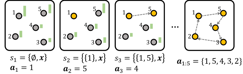
Figure 1: An example: let us have five locations to visit $\bm{x}=\{x_{1},x_{2},x_{3},x_{4},x_{5}\}$. The policy starts with the empty solution $\emptyset$, and constructs the solution by adding the next visit at each step based on the partial solution $\bm{a}_{1:t-1}$.

An example of a constructive DRL method for TSP (other CO problems can be formulated similarly) is as follows:

• States: a state $s_{t}$ is defined as a problem $\bm{x}=\{x_{i}\}_{i=1}^{N}$ that contains $N$ locations to visit and a sequence of previous actions $\bm{a}_{1:t-1}$, i.e., $\bm{s}_{t}=\{\bm{a}_{1:t-1};\bm{x}\}$.

• Actions: An action $\bm{a}_{t}$ is selecting the next visit out of unvisited locations $\{1,...,N\}\setminus\bm{a}_{1:t-1}$.

• Reward: the reward R at the final state is the negative tour length of a complete solution, i.e., $R(\bm{a}_{1:N},\bm{x})=-\sum_{i=1}^{N}||x_{\bm{a}_{i+1}}-x_{\bm{a}_{i}}||_{2}$, where $x_{\bm{a}_{i}}$ is the 2D coordination selected by action $\bm{a}_{i}$.

• Policy: The policy for the complete solution for problem $\bm{x}$ is $p_{\theta}(\bm{a}_{1:N}|\bm{x})=\prod_{t=1}^{N}p_{\theta}(\bm{a}_{t}|\bm{s}_{t})$, where $p_{\theta}(\bm{a}_{t}|\bm{s}_{t})$ is the probability of selecting action $\bm{a}_{t}$ given state $\bm{s}_{t}$.

As illustrated in Figure 1, the policy constructs a complete solution starting with an empty solution. This MDP is contextualized by $\bm{x}$ as the policy and reward highly rely on problem $\bm{x}$; thus, the trained policy differs according to the problem distribution $P(\bm{x})=P(\bm{x}|N)P(N)$. Formally, the DRL method aims to find parameter $\theta$ such that:

$$\theta^{*}=\operatorname*{arg\,max}_{\theta}\mathbb{E}_{P(N)}\mathbb{E}_{P(\bm{x}|N)}\mathbb{E}_{p_{\theta}(\cdot|\bm{x})}\left[R(\bm{a}_{1:N},\bm{x})\right]$$ (1)

Because reward function $R(\cdot)$ is non-differentiable, the REINFORCE-based method with a proper baseline for reducing variances has been utilized (Bello et al., 2017; Kool et al., 2019; Kwon et al., 2020; Kim et al., 2022). As shown in Eq. 1, the distribution $P(\bm{x})$ would affect the learned policy $p_{\theta}$. In the previous literature (Kool et al., 2019), $P(N)$ is not considered while fixing $N$ to be constant, and $P(\bm{x}|N)$ was assumed as a uniform distribution, which causes the distribution shift issue when the policy is used for solving different size of the problem (i.e., $N^{\prime}>N$).

2.2 Transfer Learning-based Adaptation Methods for DRL-CO

Active Search (AS; Bello et al., 2017) is a transfer learning method that updates the pre-trained parameters during the inference of a solution for a specific instance $\bm{x}$. Usually, the DRL model is trained to maximize rewards on the problem distribution $P(\bm{x}|N)$. Therefore, the trained model can solve an arbitrary instance $\bm{x}$ sampled from $P(\bm{x}|N)$ at the test time. However, active search improves model performance while focusing on a single instance $\bm{x}$. While active search gives promising performances, updating parameters in the test time is often inefficient and degrades practicality.

Efficient Active Search (EAS; Hottung et al., 2021) is an improved version of active search that updates a subset of parameters, not whole parameters. EAS adds new parameters dedicated to embedding and updates these parameters for the specific target problem while maintaining the rest of the parameters. This separation of the parameters’ roles allows an efficient update.

However, these methods transfer the pre-trained parameters to target problem $\bm{x}$ without utilizing prior information of distributional shift, e.g., scale gap from source to target. We observe that giving the scale priors to the transfer learning can improve transferability.

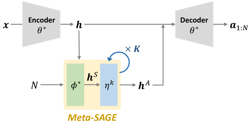
Figure 2: Structure of Meta-SAGE and test time adaptation. The scale-conditioned initial embedding $\bm{h}^{S}$ is obtained by ${\color[rgb]{0.0,0.5,0.0}g_{\phi^{*}}}(\bm{x},N)$ and the instance-wise target embedding $\bm{h}^{A}$ is obtained by ${\color[rgb]{0.0,0.2,0.55}g_{\eta^{(k)}}}(\bm{h}^{S})$. At $k$-th adaptation, $\eta^{k}$ is updated for the test instance $\bm{x}$, and other parameters (i.e., $\theta^{*}$ and $\phi^{*}$) are fixed.

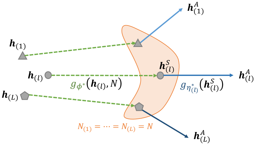
Figure 3: Transformation of embedding $\bm{h}$. SML transforms the original embedding $\bm{h}_{(l)}$ to the scale-conditioned initial embedding $\bm{h}^{S}_{(l)}=g_{\phi^{*}}(h_{(l)},N)$, where $N=N_{(l)}$. Then, $\eta^{*}_{(l)}$ is obtained via the SAGE operation with $K$ iteration for each instance. Finally, MLP $g_{\eta^{*}_{(l)}}(\bm{h}^{S}_{(l)})$ provides the target embedding $\bm{h}^{A}_{(l)}$.

3 Adaptation with Meta-SAGE

This section explains how to adapt pre-trained models with Meta-SAGE, which consists of a scale meta-learner (SML) and scheduled adaptation with guided exploration (SAGE). As shown in Figure 3, new parameters $\phi$ and $\eta$ are introduced for SML and SAGE, respectively. The multi-layer perceptron (MLP) layers $g_{\phi}(\cdot)$ and $g_{\eta}(\cdot)$ transform the the original context embedding $\bm{h}$ based on the target scale $N$, i.e., $\bm{h}^{A}=g_{\eta}(g_{\phi}(\bm{h},N))$. Note that $\phi$ is pre-trained to capture the scale information, and $\eta$ is solely updated at test time adaptation. This section focus on explaining adaptation procedure of Meta-SAGE; see Section 4 for the learning scheme for SML.

3.1 Decision Process and Guided Exploration

Decision process of DRL models.

We focus on the models utilizing the encoder-decoder structure (Vinyals et al., 2015; Bello et al., 2017; Kool et al., 2019; Kwon et al., 2020; Kim et al., 2022) where the encoder captures context embedding $\bm{h}=\{h_{i}\}_{i=1}^{N}$ of the problem $\bm{x}=\{x_{i}\}_{i=1}^{N}$, and the decoder sequentially generates action $\bm{a}_{t}$ with the context embedding $\bm{h}$ and the partial solution $\bm{a}_{1:t-1}$.

At each decision step $t$, the decoder computes the compatibility vector $\bm{u}$ to be used to select the next action. There are several strategies to compute compatibility vectors; the most popular way is to utilize multi-head attention (Vaswani et al., 2017; Kool et al., 2019; Kwon et al., 2020; Kim et al., 2022). To mask visited locations, the compatibility vector $\bm{u}$, is expressed as:

$$u_{j}=\begin{cases}u_{j}&\mbox{ if }j\notin\bm{a}_{1:t-1}\\ -\infty&\mbox{ otherwise.}\end{cases}$$

The probability $p_{i}$ for selecting location $i$ is computed by taking a SoftMax with temperature $\mathcal{T}$ as follows:

$$p_{i}=\frac{e^{u_{i}/\mathcal{T}}}{\sum_{j}e^{u_{j}/\mathcal{T}}}\quad\forall i=1,\ldots,N.$$ (2)

We provide detailed implementation of the promising encoder-decoder neural architectures of CO (Kool et al., 2019; Kwon et al., 2020; Kim et al., 2022) at Section B.1.

Guided exploration.

To encourage the policy assign more probabilities to candidates near the last action, we introduce a locality bias based on the distances. Assume that the current state is $s_{t}=\{\bm{a}_{1:t};\bm{x}\}$, and the current location is $\bm{a}_{t}$ in TSP. At each $t$, we can measure the distance between the remaining locations to visit with

$$d(x_{\bm{a}_{t}},\bm{x}):=\left\{||x_{i}-x_{\bm{a}_{t}}||;i\in\{1,\ldots,N\}\setminus\bm{a}_{1:t}\right\}.$$

We induce the policy to select locations near the last visited location by penalizing the policy logit value $u_{j}$ for the next candidate $j$ as follows:

$$u_{j}\leftarrow u_{j}-\alpha d(x_{\bm{a}_{t}},\bm{x})_{j},\mbox{ }\forall j\in\{1,\ldots,N\}\setminus\bm{a}_{1:t}.$$ (3)

The motivation for locality bias is the lack of capability for global search in the early stages of adaptation. By inducing the model to search the local area first, the exploration capability is improved.

3.2 Scheduled Adaptation

Test time adaptation.

Following Hottung et al. (2021), we update $\eta$ based on a single instance $\bm{x}$ with two objectives: reinforcement learning objective $\mathcal{J}_{RL}$ and self-imitation learning objective $\mathcal{J}_{IL}$.

$\mathcal{J}_{RL}$ is REINFORCE loss with shared baseline $b$ (Kwon et al., 2020) which is evaluated with Monte Carlo sampling $\bm{a}_{(1)},\ldots,\bm{a}_{(M)}\sim p_{\theta^{*}}(\cdot|\bm{x};\phi^{*},\eta)$ given $\theta^{*}$ and $\phi^{*}$:

$$\begin{split}&\mathcal{J}_{RL}(\eta;\bm{x})=\\ &\quad\frac{1}{M}\sum_{m=1}^{M}\left(R(\bm{a}_{(m)},\bm{x})-b\right)\cdot\log p_{\theta^{*}}(\bm{a}_{(m)}|\bm{x};\phi^{*},\eta),\\ &\quad\text{where}\quad b=\frac{1}{M}\sum_{m=1}^{M}R(\bm{a}_{(m)};\bm{x}).\end{split}$$

$\mathcal{J}_{IL}$ is self-imitation loss to maximize the log likelihood of selecting the best-sampled solution $\bm{a}_{(*)}=\operatorname*{arg\,max}\left\{R(\bm{a}_{(1)};\bm{x}),\ldots,R(\bm{a}_{(M)};\bm{x})\right\}$ as follows:

$$\mathcal{J}_{IL}(\eta;\bm{x})=\log p_{\theta^{*}}(\bm{a}_{(*)}|\bm{x};\phi^{*},\eta).$$

The total objective is then defined as:

$$\mathcal{J}_{\text{SAGE{}}}(\eta;\bm{x})=\mathcal{J}_{RL}(\eta;\bm{x})+\lambda\mathcal{J}_{IL}(\eta;\bm{x}),$$ (4)

where $\lambda$ is a tunable hyperparameter. The parameter $\eta$ is iteratively updated to maximize the total objective, i.e.,

$$\eta^{k}\leftarrow\eta^{k-1}+\delta\nabla\mathcal{J}_{\text{SAGE}},\quad k=1,\ldots,K$$

where $k$ is the adaptation iteration, and $\delta$ is a learning rate.

Scheduling.

SAGE is an enhanced EAS with locality bias and scheduling. The locality bias coefficient $\alpha$ in Eq. 15 is monotonically decreased as the model is adapted to the target instance (i.e., the adaptation step $k$ increases) as follows:

$$\alpha\leftarrow\gamma_{1}\alpha,\mbox{ where }0\leq\gamma_{1}<1.$$ (5)

It gradually reduces the reliance on locality bias, a strong inductive bias for the local view. Also, the SoftMax temperature $\mathcal{T}$ in Eq. 2 is scheduled for confidence exploitation as follows:

$$\mathcal{T}\leftarrow\gamma_{2}\mathcal{T},\mbox{ where }0\leq\gamma_{2}<1.$$ (6)

In summary, we get updated parameter via SAGE operation as illustrated in Figure 3, i.e., $\eta^{K}\leftarrow\text{SAGE{}}(\bm{x},K;\theta^{*},\phi^{*})$ for the given parameters $\theta^{*},\phi^{*}$, and the target instance $\bm{x}$.

4 Training Meta-SAGE

This section provides a formulation of Meta-SAGE and a meta-learning scheme for SML. We provide a pseudo-code in Appendix A.

4.1 Bi-level Formulation of Training Meta-SAGE

The role of SML is to give properly transformed embedding to the subsequent parameter adaptation (i.e., SAGE) based on the scale information. We formulate our training of Meta-SAGE as bi-level optimization as follows:

$$\max_{{\color[rgb]{0.0,0.5,0.0}\phi}}\quad \mathbb{E}_{P(\bm{x})}\mathbb{E}_{p_{\theta^{*}}(\cdot|\bm{x};\phi,{\color[rgb]{0.0,0.2,0.55}\eta})}\left[R(\bm{a}_{1:N},\bm{x})\right]$$ (7)

s.t. $${\color[rgb]{0.0,0.2,0.55}\eta}\leftarrow\text{SAGE{}}(\bm{x},K;\theta^{*},{\color[rgb]{0.0,0.5,0.0}\phi})$$ (8)

The upper-level optimization (i.e., training SML) in Eq. 7 contains $\eta$ that can be obtained by solving the lower-level optimization (i.e., SAGE). At the same time, the lower level requires optimized $\phi$ as an input. Therefore, the optimization problems are interrelated, making training more difficult.

4.2 Meta learning with Distillation Scheme

We propose Meta-learning with Distillation Scheme that reliably trains $\phi$, while breaking the inter-relationship between $\phi$ and $\eta$. The roles of $g_{\phi}(\bm{h}_{(l)},N)$ can be twofold:

1. Transporting the context embedding $\bm{h}_{(l)}$ to as close as possible to the instance-wise target embedding $\bm{h}^{A}_{(l)}=g_{\eta^{K}_{(l)}}(\bm{h}^{S}_{(l)})$.

2. Improving instance-wise adaptation quality with the scale-conditioned initial embedding $\bm{h}^{S}_{(l)}=g_{\phi}(\bm{h}_{(l)},N)$.

To achieve these two roles, we train SML parameter $\phi$ using the following objective:

$$\mathcal{J}_{\text{SML}}(\phi)=\mathcal{J}_{\text{distil}}(\phi)+\beta\mathcal{J}_{\text{zero}}(\phi),$$ (9)

where $\beta$ is a tunable hyperparameter. The intuition behind each objective follows.

Distillation objective. Let’s assume that instance-wise target node embedding $\bm{h}^{A}_{(l)}$ can be obtained from the contextual embedding $\bm{h}_{(l)}$ regardless of the scale conditioned node embedding if we conduct a sufficiently large number $K$ of SAGE adaptation on $\eta$ without SML parameters $\phi^{*}$, i.e., $\bm{h}^{A}_{(l)}=g_{\eta^{K}_{(l)}}(\bm{h}_{(l)})$, where $\eta^{K}_{(l)}\leftarrow\text{SAGE{}}(\bm{x},K;\theta^{*})$. Then, given $\bm{x}_{(l)}\sim P(\bm{x}|N)P(N)$ for $l=1,\ldots,L$, we can amortize $g_{\phi}(\bm{h}_{(l)},N)$ to imitate $g_{\eta^{K}_{(l)}}(\bm{h}_{(l)})$, which is referred to as distillation. This can be done by maximizing the following objective:

$$\mathcal{J}_{\text{distil}}(\phi)=-\frac{1}{L}\sum_{l=1}^{L}\|g_{\phi}(\bm{h}_{(l)},N_{(l)})-g_{\eta^{K}_{(l)}}(\bm{h}_{(l)})\|_{2}$$ (10)

with sufficiently large $K$. Note that by maximizing $\mathcal{J}_{\text{distil}}(\phi)$, the distance between the scale-conditioned embedding $\bm{h}^{S}_{(l)}$ and the instance-wise target embedding decreases so that

$$\bm{h}^{S}_{(l)}=g_{\phi}(\bm{h}_{(l)},N_{(l)})\approx\mathbb{E}_{P(\bm{x}|N=N_{(l)})}g_{\eta^{K}_{(l)}}(\bm{h}_{(l)}).$$

That is, SML is trained to convert context embedding to the expected target embedding $\bm{h}_{(l)}^{T}=g_{\eta^{K}_{(l)}}(\bm{h}_{(l)})$ for the problem instances $\bm{x}_{(l)}\sim P(\bm{x}|N)P(N)$ for $l=1,\ldots,L$.

Zero-shot simulation objective. We hope that the scale-conditioned initial embedding $\bm{h}^{S}=g_{\phi}(\bm{h},N)$ to be a sufficiently good representation to solve a target problem instance $\bm{x}$ even before $\bm{h}^{S}$ is transformed to the instance-wise target embedding $\bm{h}^{A}$. Thus, it can be interpreted as the input $\bm{h}^{S}$ is the $0$-th adapted target embedding (i.e., SAGE with $K=0$). Based on this interpretation, we define the zero-adaptation objective as follows:

$$\mathcal{J}_{\text{zero}}(\phi)=\mathbb{E}_{\bm{x}\sim P(\bm{x}|N)P(N)}\left[\mathcal{J}_{\text{SAGE}}(\phi;\bm{x})\right].$$

The SAGE objective function $\mathcal{J}_{\text{SAGE}}$ is contextualized by $\bm{x}$. By taking an expectation over the problem distribution, the shared parameter $\phi$ is trained over the problem distribution $P(\bm{x}|N)P(N)$.

Table 1: Performance evaluation results for the four CO tasks of TSP, CVRP, PCTSP, and OP are presented. We used two pre-trained DRL models, POMO and Sym-NCO (termed Sym. in the table), and deployed adaptation methods on each. The best-performing method is highlighted in bold among adaptation methods and marked as $*$ if the method outperforms the problem-specific solver. Note that OP is a maximization problem (i.e., the objective value is higher ($\uparrow$), the better), while others are minimization problems (i.e., the objective value is lower ($\downarrow$), the better). The reported time is for solving whole instances.

			$N=200$ ($1$K Instances)			$N=500$ ($128$ Instances)			$N=1,000$ ($128$ Instances)
			Obj.	Gap	Time	Obj.	Gap	Time	Obj.	Gap	Time
TSP ($\downarrow$)	Concorde		10.687	0.000%	0.4H	16.542	0.000%	0.6H	23.139	0.000%	5.4H
	POMO	AS	10.735	0.449%	22.4H	17.335	4.791%	9.2H	-	-	-
		EAS	10.736	0.455%	2.4H	18.135	9.362%	4.3H	30.744	32.869%	20H
		SBGS	10.734	0.436%	2.1H	18.191	9.963%	4.2H	28.413	22.795%	19H
		Ours	10.729	0.391%	2.1H	17.131	3.559%	3.8H	25.924	12.038%	18H
	Sym.	AS	10.748	0.575%	22.4H	17.352	4.897%	9.2H	-	-	-
		EAS	10.731	0.413%	2.4H	18.194	9.986%	4.3H	31.241	35.017%	20H
		SBGS	10.730	0.402%	2.1H	18.193	9.98%	4.2H	28.431	22.87%	19H
		Ours	10.728	0.387%	2.1H	17.095	3.339%	3.8H	25.798	11.488%	18H
CVRP ($\downarrow$)	LKH3		22.003	0.000%	25H	63.299	0.000%	16H	120.292	0.000%	40H
	POMO	AS	22.050	0.213%	28.2H	64.053	1.192%	11.5H	-	-	-
		EAS	22.023	0.091%	3.1H	64.318	1.610%	5.5H	125.043	3.95%	24H
		SBGS	22.015	0.055%	3.1H	65.211	3.02%	5.2H	126.554	5.206%	20H
		Ours	22.001*	-0.009%*	2.7H*	63.322	0.035%	4.7H	121.114	0.683%	20H
	Sym.	AS	21.955*	-0.218%*	28.2H	63.308	0.015%	11.5H	-	-	-
		EAS	22.038	0.159%	3.1H	64.256	1.511%	5.5H	124.711	3.674%	24H
		SBGS	22.029	0.116%	3.1H	65.163	2.945%	5.2H	126.208	4.918%	20H
		Ours	21.982	-0.094%	2.7H*	63.281*	-0.028%*	4.7H*	121.116	0.685%	20H
PCTSP ($\downarrow$)	OR-Tools		7.954	0.000%	16.7H	12.201	0.000%	2.1H	23.611	0.000%	2.1H
	Sym.	AS	7.325	-7.8%	3.5H	11.589	-5.013%	2H	17.172	-27.273%	3.9H
		EAS	7.335*	-7.781%*	9M*	12.369	1.378%	5.4M	21.076*	-10.737%*	0.3H*
		Ours	7.299*	-8.236%*	6.6M*	11.175*	-8.412%*	3.7M*	16.219*	-31.31%*	0.2H*
OP ($\uparrow$)	Compass		49.216	0.000%	20.9M	97.323	0.000%	11M	161.682	0.000%	48.8M
	Sym.	AS	48.946	0.548%	2.8H	97.696	-0.382%	1.1H	154.233	4.607%	1.7H
		EAS	48.849	0.746%	7.2M	85.032	12.63%	2.8M	107.75	33.357%	7.4M
		Ours	49.05	0.337%	5.4M	98.762*	-1.457%*	2.2M*	154.307	4.562%	6.5M

5 Experimental Results

This section provides experimental results to validate Meta-SAGE with two pre-trained DRL models on four CO tasks. See Appendix B for the details of implementation.

DRL models for adaptation. Our new adaptation method is deployed to two representative DRL models for CO: Policy Optimization for Multiple Optima (POMO; Kwon et al., 2020) and Symmetric Neural Combinatorial Optimization (Sym-NCO; Kim et al., 2022). We use the pre-trained models on $N=100$ published online; thus, the performance of these two models is supposed to be not good on larger-scale instances without adaptation.

CO Tasks. We target four CO tasks: the traveling salesman problem (TSP), the capacitated vehicle routing problem (CVRP), the Prize Collecting TSP (PCTSP), and the orienteering problem (OP). The tasks are known as NP-hard (Garey & Johnson, 1979).

• The TSP is to find the shortest route for a salesman to visit every city and return to the first city, also known as a Hamiltonian cycle with minimum distances.

• The CVRP (Dantzig & Ramser, 1959) is a variation of the TSP that assumes multi-vehicles with limited capacity. CVRP aims to find the set of tours each of which starts from the depot, visits cities once, and returns to the depot and the union of the tours covers all cities while minimizing the total distances.

• In PCTSP (Balas, 1989), each city has a prize and penalty; thus, the salesman gets prizes for visiting the cities and penalties for the unvisited cities. PCTSP minimizes the total length of the route and the net penalties while collecting at least the minimum prizes.

• Lastly, the OP (Golden et al., 1987) also considers prizes associated with visiting. The goal is to find a route that maximizes the prizes from visited cities while keeping the length of the route shorter than a given maximum distance.

POMO and Sym-NCO models are pre-trained on TSP and CVRP, and Sym-NCO is additionally pre-trained on PCTSP and OP. Note that these TSP variant problems are highly challenging.

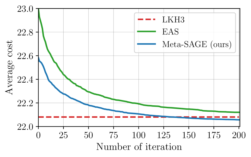
(a) $N=200$

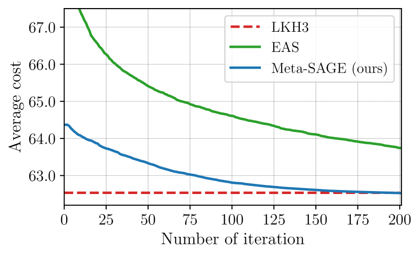
(b) $N=500$

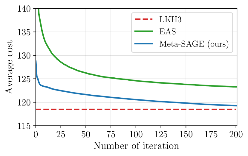
(c) $N=1,000$

Figure 4: Adaptation performance on CVRP with pre-trained Sym-NCO compared to LKH3.

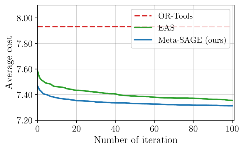
(a) $N=200$

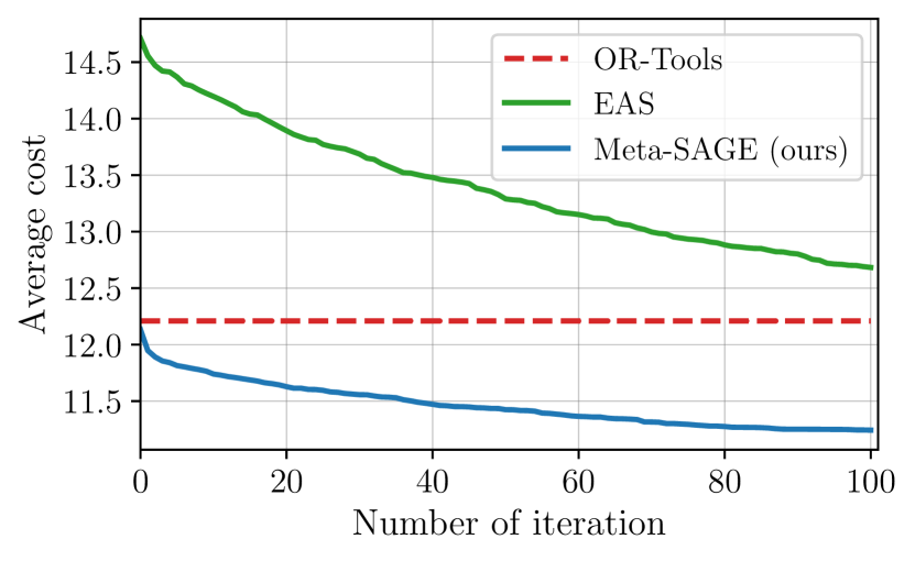
(b) $N=200$

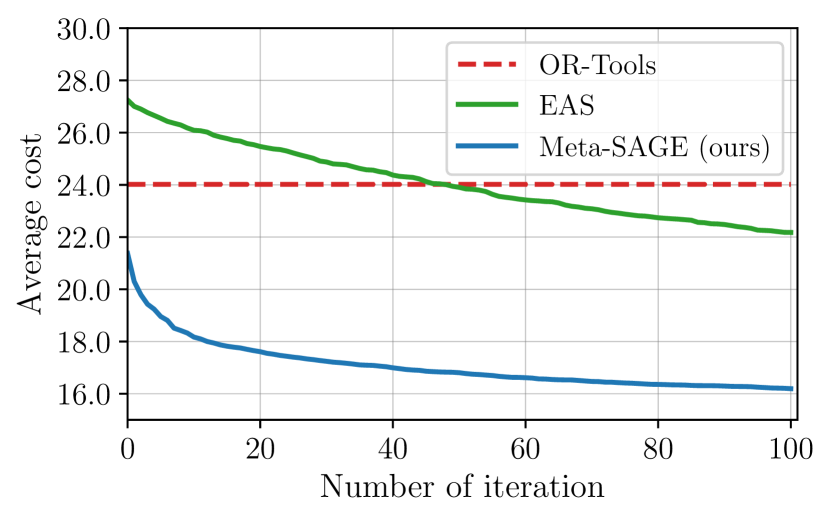
(c) $N=1,000$

Figure 5: Adaptation performance on PCTSP with pre-trained Sym-NCO compared to OR-Tools.

Baselines. We consider three baselines for test time adaptation: active search (AS; Bello et al., 2017), Efficient Active Search (EAS; Hottung et al., 2021) and Simulation Guided Beam Search with EAS (SGBS; Choo et al., 2022). We describe the details of implementation in Appendix C.

Performance metric. We measure the Baseline Gap using state-of-the-art solvers for each task. As baseline solvers, we employ Concorde (David Applegate & Cook, 2023) for TSP, LKH3 (Helsgaun, 2017) for CVRP, OR-Tools (Perron & Furnon, 2019) for PCTSP, and Compass (Kool et al., 2019) for OP.

Computation resources and runtime. We used a single NVIDIA A100 40GB VRAM GPU and an Intel Scalable Gold CPU for the experiments. We terminate EAS and SGBS when the runtime exceeds the runtime of Meta-SAGE with $200$ iterations. Since AS is unavailable to process in batch, we conduct 200 iterations for adaptation, the same as ours for each instance. We measure the time taken to solve whole instances following Hottung et al. (2021).

5.1 Main Results

As shown in Table 1, Meta-SAGE outperforms other adaptation baselines except for Sym-NCO on CVRP with 200. The results show that our method improves the pre-trained DRL models with EAS in consistency. Surprisingly, Meta-SAGE finds better solutions than the heuristic solver on CVRP with $N=200,500$, PCTSP with every scale, and OP with $N=500$. Note that heuristic solvers are designed for each problem class and are highly engineered.

It is noteworthy that Meta-SAGE transforms the pre-trained model to outperform the task-specific heuristic solver.

Figure 4 and Figure 5 illustrate the cost obtained by EAS and Meta-SAGE with respect to the adaptation iteration on CVRP and PCTSP. The results clearly show that our method achieves improved performances compared to EAS with the same number of iteration (i.e., improved transferability). For example, on CVRP with $N=200,500$, Meta-SAGE outperforms LKH3 with 200 iterations, whereas EAS still gives higher costs than LKH3. Noticeably, our initial (i.e., zero-shot) cost is lower than EAS in every instance, meaning that SML gives the scale-conditioned initial embedding $\bm{h}^{S}$ by appropriately transforming the original context embedding $\bm{h}$ before parameter adaptation. See Section D.1 for the results of TSP and OP.

5.2 Real-world Benchmark

Table 2: Evaluation of adaptation methods with pre-trained Sym-NCO on the real-world CVRP dataset. We report average values according to the range of instance scale $N$ between $500$ and $1,000$. The full results are provided in Section D.2.

Range	LKH3	Sym-NCO
		EAS	Ours
$500\leq N<600$	92,095	95,384	94,028
$600\leq N<700$	85,453	88,987	87,372
$700\leq N<800$	89,009	92,288	90,184
$800\leq N<900$	112,785	119,332	116,096
$900\leq N\leq 1000$	150,332	175,999	172,916

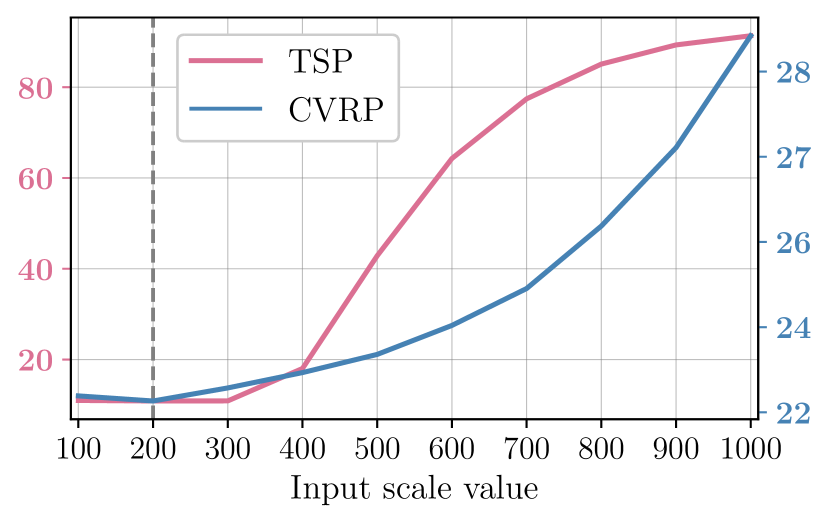
(a) $N=200$

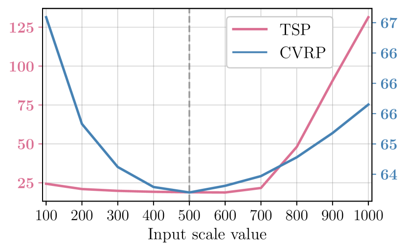
(b) $N=500$

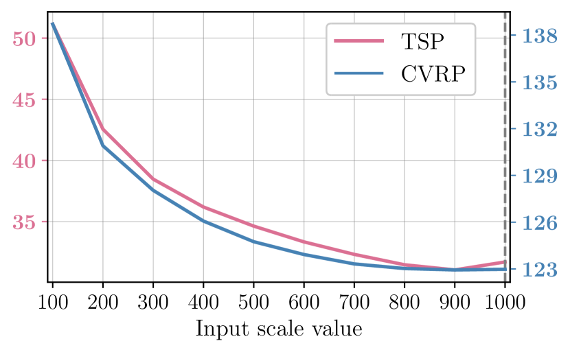
(c) $N=1,000$

Figure 6: Scale matching performance of SML. For each target scale of $N=200,500,1000$, SML gives lower cost (i.e., better performances) when the input scale $N^{\prime}$ is closer to the actual target scale.

We apply our method on the real-world dataset for CVRP, X-instances in CVRPLIB (Uchoa et al., 2017). The model is trained with CVRP instances whose demands and locations are samples from uniform distributions. On the other hand, the X-instances are generated by various demand and location distributions to cover real-world applications. As shown in Table 2, Meta-SAGE outperforms EAS in every range. Moreover, the real-world experiment demonstrates that our method can overcome the distribution shift.

5.3 Ablation Study

Table 3: Ablation study for Meta-SAGE component. LB and Temp. refer to locality bias and SoftMax temperature, respectively.

SML	SAGE			Tasks
	LB	Sche. LB	Sche. Temp.	TSP	CVRP
				18.63	63.97
✓				17.70	63.17
✓	✓			17.68	63.10
✓	✓	✓		17.67	63.07
✓	✓	✓	✓	17.22	62.69

Effectiveness of main components. Meta-SAGE consists of SML and SAGE composed of guided exploration with locality bias and scheduling. The SAGE has two scheduling targets, locality bias and SoftMax temperature. The performances are measured while ablating each element. The experiments are conducted on TSP and CVRP with $N=500$, using the Sym-NCO as a pre-trained DRL model. Each component significantly impacts performance improvement, as shown in the Table 3.

Effectiveness of SML. The objective of SML is to support SAGE by providing proper scale-conditioned initial embedding $\bm{h}^{S}=g_{\phi}(\bm{h},N)$ based on the scale information. To verify SML’s effect, we measure the $L1$ distance between the input and output embedding of SAGE. The effectiveness can be demonstrated by the reduced distance by SML, i.e.,

$$||\bm{h}^{S}-\bm{h}^{A}||<||\bm{h}-\bm{h}^{A}||.$$

Table 4: The $L1$ distance between input and output embedding of SAGE. The distances are measured with and without SML using Sym-NCO.

	TSP ($N=500$)	CVRP ($N=500$)
w/ SML	7,175.99	9,285.22
w/o SML	8,066.13	10,361.51

As shown in Table 4, SML reduces the distance between the initial and target embedding of SAGE, which verifies that SML provides effective initial embedding for SAGE.

Scale matching abilities of SML. Meta-SAGE improves adaptation efficiency by capturing scale information via SML. Therefore, the best performance of SML should be obtained when the scale input matches the target scale. Figure 6 illustrates that SML performs well when the input scales are close to the actual target scale.

Effectiveness of objective components in SML. We verify the effectiveness of two objective function in Eq. 9; empirical results can be found in Figure 9(c).

6 Discussion

6.1 Other Meta-learning for CO

Qiu et al. (2022) suggested Differentiable Meta Solver for Combinatorial Optimization Problems (DIMES) by utilizing the model agnostic meta-learning (MAML; Finn et al., 2017) to compensate for instance-wise search.

The difference is that we focus more on scale transferability, which is beneficial when the model is unavailable to be pre-trained on large scales. Our approach utilizes already trained (i.e., not meta-trained) models and adapts them to unseen tasks by considering scale prior. In addition, our method can be orthogonally applied with pre-trained DIMES for further improvements.

6.2 Extension to Non-Euclidean Graph CO

We verified that Meta-SAGE achieves promising performances on large-scale Euclidean CO problems by adapting the pre-trained model. However, several important problems, such as scheduling, are non-Euclidean CO, whose edge values cannot be obtained with node values. Meta-SAGE can be extended by being attached to promising pre-trained models for non-Euclidean CO; we leave it as further work.

6.3 Distributional Shifts

This work focuses on the distributional shift of problem scale. However, the robustness for other distributional shifts, including instance distribution, is required to make DRL solvers more practical, especially when they are trained with fixed known distributions. Despite several prior research (Jiang et al., 2022; Xin et al., 2022; Bi et al., 2022), tackling distributional shifts remains challenging. Our additional experiments on real-world CVRP benchmarks show the feasibility of Meta-SAGE on instance-wise distributional shifts. We expect that Meta-SAGE can consider other distributional shifts, not only scale.

6.4 Mathematical Programming

While neural combinatorial optimization (NCO) approaches provide near-optimal solutions with fast computation, it cannot be claimed that they exhibit superiority over mathematical programming approaches such as branch-and-bound. Unlike NCO, mathematical programming-based approaches, such as branch-and-bound, are theoretically guaranteed to find optimal solutions. Since current NCO solvers cannot guarantee optimal solutions or provable optimality gaps, the theoretical study of NCO remains a challenging and significant area for future exploration.

Appendix A Trainig Algorithm for Meta-SAGE

Algorithm 1 Meta-SAGE

  Set $\theta^{*}\leftarrow\text{pretrained model parameter}$, $\phi$: SML parameter.

  A. Meta-Learning SML $\phi$

  for $t=1.,,,.T$ do

     $\mathcal{J}_{\text{zero}}\leftarrow$ Zero-shot simulation objective of SAGE

     $\mathcal{J}_{\text{distil}}\leftarrow$ Distil. Objective with pre-sim. of SAGE

     Train $\phi\leftarrow\phi_{t}$ to maximize $\mathcal{J}_{distil}+\beta\mathcal{J}_{\text{zero}}$

  end for

  Set $\bm{x}_{\text{test}}$, where $N$ is large. Set $\eta$ is a test-time learnable parameter. Set $\mathcal{T}$: initial SoftMax temperature. Set $\alpha$: initial locality bias level.Set $0<\gamma_{1}<1$ and $0<\gamma_{2}<1$ are decaying factors.Set $f_{\theta^{*}}(\bm{x})$ as the pre-trained encoder.Set $p_{\theta^{*}}(\bm{a}|\bm{h};\mathcal{T},\alpha)$ as the pre-trained decoder.Set $g_{\phi^{T}}(\bm{h},N)$ as the trained SML.

  B. Test-time Adaptation with SAGE

  for $k=1.,,,.K$ do

     $\bm{h}\leftarrow f_{\theta^{*}}(\bm{x};\theta^{*})$: Context embedding from Encoder.

     $\bm{h}\leftarrow g_{\phi^{T}}(\bm{h},N)$: SML’s Context Transformation.

     $\bm{h}\leftarrow g_{\eta}(\bm{h})$: Test-time Context Transformation

     $\bm{a}^{1},...,\bm{a}^{M}\sim p_{\theta^{*}}(\cdot|\bm{h};\mathcal{T},\alpha)$: MC sampling

     $\mathcal{J}_{RL}\leftarrow$ REINFORCE objective with shared baseline

     $\mathcal{J}_{IL}\leftarrow$ Self Imitation objective

     Train $\eta\leftarrow\eta_{k}$ to maximize $\mathcal{J}_{RL}+\lambda\mathcal{J}_{IL}$

     Scheduling: $\alpha\leftarrow\gamma_{1}\alpha$, $\mathcal{T}\leftarrow\gamma_{2}\mathcal{T}$,

  end for

Appendix B Implementation Details of Meta-SAGE

B.1 Architecture of Target Model

In this research, we focus on two representative DRL models, POMO (Kwon et al., 2020) and Sym-NCO (Kim et al., 2022). Both models have a similar neural architecture, based on the attention model (Kool et al., 2019, AM). The main difference between these models is the training method for the AM.

The AM has a transformer-style encoder-decoder structure, where the encoder $f_{\text{enc}}(\bm{x})$ creates a context embedding $\bm{h}$ and the decoder $p_{\text{dec}}(\bm{h})$ generates action sequences $\bm{a}_{1:N}$ in an auto-regressive manner. The architecture of the encoder is not discussed here as our method and EAS (Hottung et al., 2021) focus on $\bm{h}$ for the decoding scheme. For more information on the encoder architecture, refer to (Kool et al., 2019).

The decoder $p_{\text{dec}}(\bm{h})$ is an auto-regressive process, which produces $\bm{a}t$ by referring to previously selected actions $\bm{a}_{1:t-1}$. Specifically, $\bm{h}$ is transformed into key $\bm{K}$ and value $\bm{V}$ via linear projection.

$$\bm{K}=\Phi_{\text{linear},k}(\bm{h}),\quad\bm{V}=\Phi_{\text{linear},v}(\bm{h})\text{. }$$

Then the contextual query $q_{c}$ is computed as follows:

$$\bm{q}_{c}=\frac{1}{N}\sum_{i=1}^{N}{\bm{h}_{i}}+\bm{h}_{\text{depot}}+\bm{h}_{\bm{a}_{t-1}}\text{. }$$

The $h_{\text{depot}}$ indicates the embedding of the depot node, and $\bm{h}_{\bm{a}_{t-1}}$ indicates the embedding of the previously selected action. Then we can compute compatibility $u_{j}$ as:

$$u_{j}=\begin{cases}C\tanh\left(\frac{q_{c}^{T}K_{j}}{\sqrt{d_{k}}}\right)&\mbox{ if }j\notin\bm{a}_{1:t-1}\\ -\infty&\mbox{ otherwise.}\end{cases}$$ (11)

Using compatibility, we can compute attention weight as:

$$a_{j}=\frac{e^{u_{j}}}{\sum_{j^{\prime}}e^{u_{j^{\prime}}}}\text{. }$$

Then finally, the contextual query is updated as:

$$\mathbf{q}^{*}_{c}=\sum_{j}a_{j}\mathbf{v}_{j}\text{. }$$ (12)

Then finally, the compatibility for selecting the next action is computed the same with Eq. 13 but using $\mathbf{q}^{*}_{c}$:

$$u^{*}_{j}=\begin{cases}C\tanh\left(\frac{\mathbf{q}^{*^{T}}_{c}K_{j}}{\sqrt{d_{k}}}\right)&\mbox{ if }j\notin\bm{a}_{1:t-1}\\ -\infty&\mbox{ otherwise.}\end{cases}$$ (13)

Finally, the probability to select $\bm{a}_{t}$ is computed with compatibility $u^{*}_{j}$ using SoftMax function:

$$p(\bm{a}_{t}=i|\bm{a}_{1:t-1};\bm{x})=p_{i}=\frac{e^{u^{*}_{i}/\mathcal{T}}}{\sum_{j}e^{u^{*}_{j}/\mathcal{T}}}\quad\forall i=1,\ldots,N.$$ (14)

B.2 Implementation of SML

We employ a 2-layer MLP with 128 hidden dimensions to match the scale N with the embedding $\bm{h}$. The sum of these vectors is then input into another 2-layer MLP with ReLU activation to parameterize the SML, $g_{\phi}(\bm{h},N)$ with parameters $\phi$. For the test time adaptation, we employ a 2-layered MLP with ReLU activation for $g_{\eta}(\bm{h})$, which has 128 hidden dimensions, 128 input dimensions, and 128 output dimensions.

To train the SML, we leverage both distillation and zero-shot simulation objectives. Distillation uses $\{\bm{h}_{(l)}\}_{l=1}^{L}$ where $L=4,000$ and instances $\bm{x}_{(l)}$ uniformly sampled for $N=200,300,400$. The zero-shot simulation objective uses the same instances as the distillation process. We only used sparse data with a moderate scale to verify that our method can be trained in limited environments and can be useful in harsher, practical settings.

B.3 Implementation of SAGE for Target Neural Architectures

The SAGE algorithm is similar to EAS(Hottung et al., 2021), but with different scheduling of locality bias and SoftMax temperature. EAS aims to tune $\bm{h}$, but for memory efficiency during inference, it only focuses on a subset of $\bm{h}$, specifically $\bm{q}_{c}^{*}$. The learnable parameter $\eta$ is trained for this purpose:

$$\bm{q}_{c}^{*}\leftarrow\bm{q}_{c}^{*}+g_{\eta}(\bm{q}_{c}^{*})$$

Where $g_{\eta}$ is a multi-layer perceptron of parameter $\eta$ with ReLU activation. The novel part of SAGE is locality bias and temperature scaling.

Locality bias and scheduling. The locality bias, we utilize distance between current node $x_{\bm{a}_{t}}$ and candidate nodes:

$$d(x_{\bm{a}_{t}},\bm{x}):=\left\{||x_{i}-x_{\bm{a}_{t}}||;i\in\{1,\ldots,N\}\setminus\bm{a}_{1:t}\right\}.$$

Then we penalize compatibility of high-distance nodes (i.e., compensate local-distance nodes):

$$u^{*}_{j}\leftarrow u^{*}_{j}-\alpha d(x_{\bm{a}_{t}},\bm{x})_{j},\mbox{ }\forall j\in\{1,\ldots,N\}\setminus\bm{a}_{1:t}.$$ (15)

The reliance of locality bias $\alpha$ is decaying as learning iteration $K$ is increasing:

$$\alpha\leftarrow\gamma_{1}\alpha,\mbox{ where }0\leq\gamma_{1}<1.$$ (16)

SoftMax scaling. The SoftMax temperature $\mathcal{T}$ for Eq. 14 is initially set to a high value for exploration and gradually lowered as training progresses for better exploitation:

$$\mathcal{T}\leftarrow\gamma_{2}\mathcal{T},\mbox{ where }0\leq\gamma_{2}<1.$$ (17)

B.4 Hyperparameters for Training

In the training of the SML model, the ADAM optimizer as described by (Kingma & Ba, 2015) is utilized with a learning rate of $10^{-3}$ and a coefficient of $\beta=1$ for the zero-shot simulation loss $\mathcal{J}_{\text{distil}}(\phi,N)$. Test-time adaptation is performed using the SAGE method, where the initial temperature is set to $\mathcal{T}=1.0$ and scheduled to decrease to $\mathcal{T}=0.3$ after $K=200$ iterations of decay (i.e., $\delta_{1}^{K}=0.3$), where $K$ represents the number of iterations. The initial reliance level of the locality bias is set to $\alpha=1$ and scheduled to decrease to $\alpha=0.3$ after $K=200$ iterations of decay (i.e., $\delta_{2}^{K}=0.3$). The value of $K$ is set to 200 for TSP and CVRP, and 100 for PCTSP and OP. An augmentation technique described by (Kwon et al., 2020) is implemented to boost solution quality, so we sampled $N\times A$ solutions from the DRL model, where $N$ represents the scale of the problem and $A$ represents the number of augmentations. The number of augmentations, $A$, is adjusted according to the scale of the problem, $N$. The parameter $\eta$ is learned using $\mathcal{J}_{\text{SAGE}}$ and the final solution is chosen as the best solution among the $K\times N\times A$ solutions. Test-time adaptation is performed using the ADAM optimizer with a learning rate as specified in the open source code by (Hottung et al., 2021). The weight of the self-imitation learning objective is set to $\lambda=0.005$.

B.5 Instance generation and evaluation metric

Instance generation. We generate training and test instances following Kool et al. (2019), like many works in NCO (Kwon et al., 2020; Kim et al., 2022; Hottung et al., 2021).

• TSP: ($x,y$) coordination of each node is randomly sampled to obtain a uniform distribution within the range of $[0,1]$.

• CVRP: ($x,y$) coordination of each node is uniformly distributed within $[0,1]$, while the demand of each node is sampled from the uniform distribution within the range of $[1,9]$.

• PCTSP: ($x,y$) coordination and the penalty of each node is sampled from the uniform distribution within the range of $[0,1]$.

• OP: ($x,y$) coordination of each node is randomly sampled to obtain a uniform distribution within $[0,1]$. Furthermore, each node’s price ($\rho_{i}$) is determined based on its distance to the depot ($\rho_{i}=1+\lfloor 99\cdot\frac{d_{0i}}{max_{j=1}^{n}d_{0j}}\rfloor$), such that it increases with distance.

Evaluation metric. We measure the performance using baseline solvers for each task. Note that this is not an optimality gap since these baselines are not exact methods except for Concorde, which is based on the cutting plane method. Precisely, (Performance) Gap is computed as

$$\text{Performance Gap}=\frac{obj-obj_{B}}{obj_{B}}\times 100(\%),$$

where $obj$ is the objective value of DRL methods, and $obj_{B}$ is the objective value from baseline solvers (Concode, LKH3, OR-Tools, and Compass).

Appendix C Implementation Details of Baselines

C.1 Active Search

Active Search is tuning all parameters of a model to a target instance. For TSP and CVRP, we follow the learning rate hyperparameter instruction of open source code by (Hottung et al., 2021).

	TSP	CVRP	PCTSP	OP
Learning rate	2.6e-4	2.6e-5	2.6e-4	2.6e-4

Table 5: Hyperparameter setting for active search.

C.2 Efficient Active Search

Efficient Active Search(EAS) inserts the layers into the model and updates the layers of parameters. We follow the position of inserted layer and hyperparameter, same with open source code by (Hottung et al., 2021) except the imitation rate, batch size, and augmentation size, which are the same as our method.

	TSP	CVRP	PCTSP	OP
Learning rate	3.2e-3	4.1e-3	1e-3	1e-3
Imitation rate	5e-3	5e-3	5e-3	5e-3

Table 6: Hyperparameter setting for efficient active search.

C.3 Simulation Guided Beam Search with EAS

Simulation Guided Beam Search(SGBS) with EAS is combined SGBS with EAS. We follow the position of inserted layer and hyperparameter, same with open source code by (Choo et al., 2022) except the batch size, and augmentation size, which are the same as our method.

	TSP	CVRP
Learning rate	8.15e-3	4.1e-3
Imitation rate	6e-3	5e-3
Beam width	10	4
Rollout per node	9	3
EAS iteration	1	1

Table 7: Hyperparameter setting for simulation guided beam search with eas.

Appendix D Additional Experiments

D.1 Adaptation Performance of TSP and OP

Figure 7 and Figure 8 depict the cost obtained by the EAS method and our proposed method with respect to the number of adaptation iterations on TSP and OP tasks, respectively. The results demonstrate that our method enhances the performance across all scales and tasks with the same number of iterations compared to EAS. Specifically, for the OP task with $N=500$, our method outperforms Compass, a problem-specific solver, with 100 iterative adaptations.

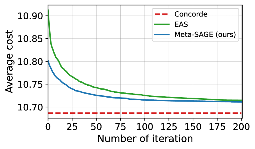
(a) $N=200$

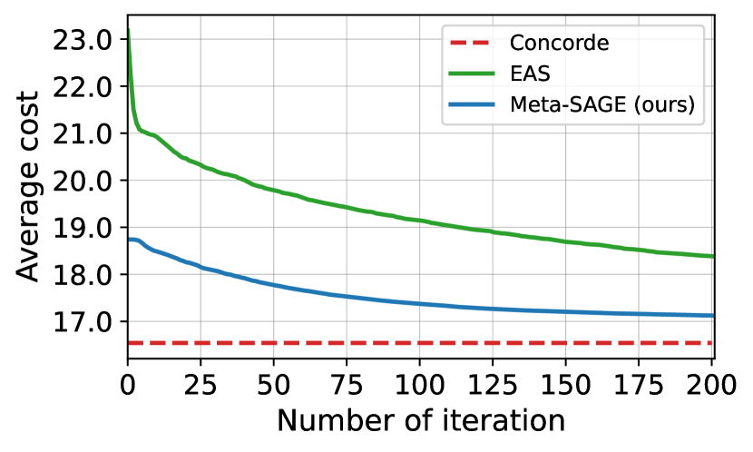
(b) $N=500$

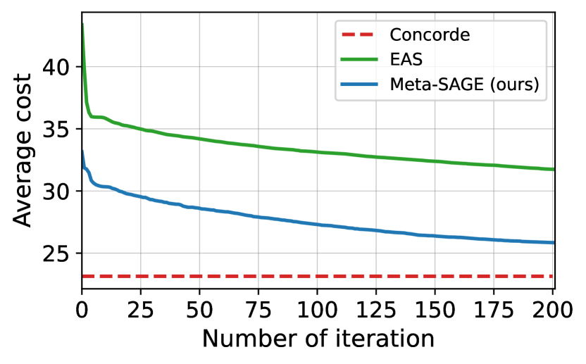
(c) $N=1,000$

Figure 7: Adaptation performance on TSP with pre-trained Sym-NCO compared to Concorde.

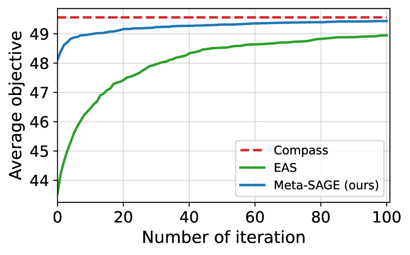
(a) $N=200$

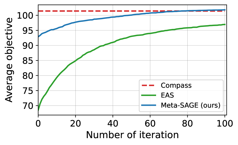
(b) $N=500$

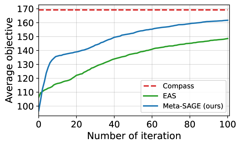
(c) $N=1,000$

Figure 8: Adaptation performance on OP with pre-trained Sym-NCO compared to Compass.

D.2 Full results for X-instances in CVRPLIB

The dataset consists of $100$ instances with a scale range from $100$ to $1,000$. We provide the full experimental result below.

Table 8: Evaluation of adaptation methods on the real-world CVRP dataset. We report average values according to the range of instance scale $N$.

Range	LKH3	Sym-NCO
		EAS	Ours
$100\leq N<200$	25,827	26,196	26,169
$200\leq N<300$	41,956	42,553	42,392
$300\leq N<400$	56,588	57,675	57,245
$400\leq N<500$	76,087	78,316	77,238
$500\leq N<600$	92,095	95,384	94,028
$600\leq N<700$	85,453	88,987	87,372
$700\leq N<800$	89,009	92,288	90,184
$800\leq N<900$	112,785	119,332	116,096
$900\leq N\leq 1000$	150,332	175,999	172,916

D.3 Effectiveness of Objective Function Components in Training SML

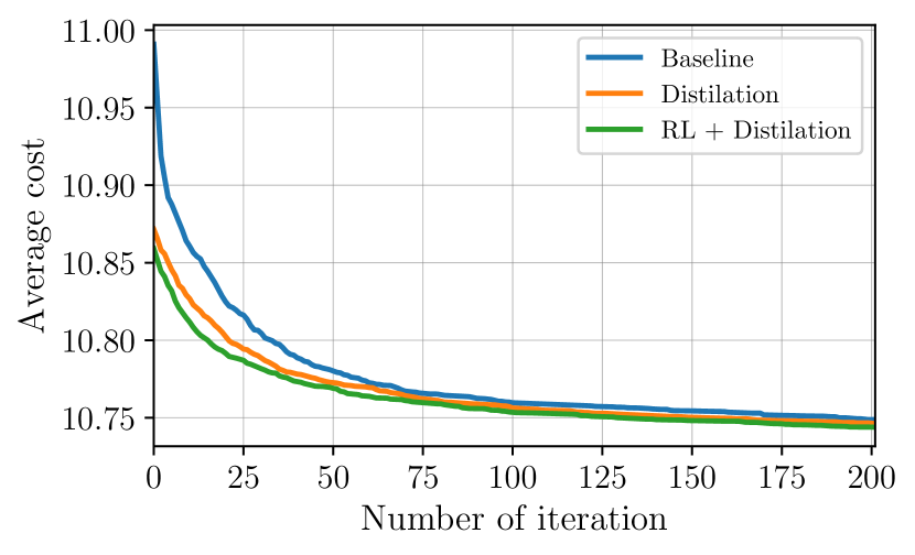
(a) $N=200$

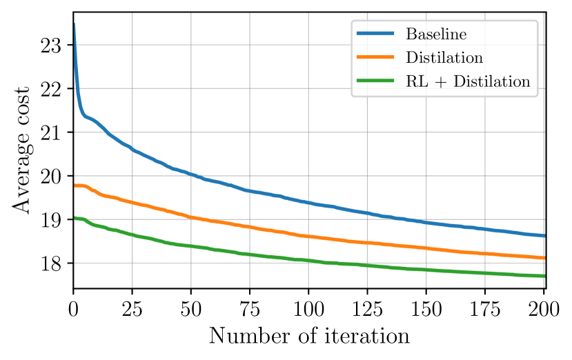
(b) $N=500$

(c) $N=1,000$

Figure 9: Ablation study for SML componets

We evaluated the effectiveness of each component of the distillation objective and RL objective (i.e., $\mathcal{J}_{\text{zero}}$) by analyzing the performance improvements. The results in Figure 9(c) clearly show that each component contributed to improved performance. The effectiveness increased as the scale $N$ increased, indicating that our SML successfully mitigates distributional shifts on a larger scale. Additionally, $\mathcal{J}_{\text{zero}}$, which is designed to increase zero-shot capability, was verified to significantly improve the performance in zero-shot scenarios (i.e., $K=0$), especially on $N=1000$.

References

- Ahn et al. (2020) Ahn, S., Seo, Y., and Shin, J. Learning what to defer for maximum independent sets. In III, H. D. and Singh, A. (eds.), Proceedings of the 37th International Conference on Machine Learning, volume 119 of Proceedings of Machine Learning Research, pp. 134–144. PMLR, 13–18 Jul 2020. URL http://proceedings.mlr.press/v119/ahn20a.html.
- Balas (1989) Balas, E. The prize collecting traveling salesman problem. Networks, 19(6):621–636, 1989.
- Barrett et al. (2020) Barrett, T., Clements, W., Foerster, J., and Lvovsky, A. Exploratory combinatorial optimization with reinforcement learning. In Proceedings of the AAAI Conference on Artificial Intelligence, volume 34, pp. 3243–3250, 2020.
- Bello et al. (2017) Bello, I., Pham, H., Le, Q. V., Norouzi, M., and Bengio, S. Neural combinatorial optimization with reinforcement learning, 2017.
- Bi et al. (2022) Bi, J., Ma, Y., Wang, J., Cao, Z., Chen, J., Sun, Y., and Chee, Y. M. Learning generalizable models for vehicle routing problems via knowledge distillation. In Advances in Neural Information Processing Systems, 2022.
- Caserta & Voß (2014) Caserta, M. and Voß, S. A hybrid algorithm for the dna sequencing problem. Discrete Applied Mathematics, 163:87–99, 2014.
- Chen & Tian (2019) Chen, X. and Tian, Y. Learning to perform local rewriting for combinatorial optimization. In Advances in Neural Information Processing Systems, 2019.
- Choo et al. (2022) Choo, J., Kwon, Y.-D., Kim, J., Jae, J., Hottung, A., Tierney, K., and Gwon, Y. Simulation-guided beam search for neural combinatorial optimization. arXiv preprint arXiv:2207.06190, 2022.
- da Costa et al. (2020) da Costa, P. R. d. O., Rhuggenaath, J., Zhang, Y., and Akcay, A. Learning 2-opt heuristics for the traveling salesman problem via deep reinforcement learning. In Pan, S. J. and Sugiyama, M. (eds.), Proceedings of The 12th Asian Conference on Machine Learning, volume 129 of Proceedings of Machine Learning Research, pp. 465–480, Bangkok, Thailand, 18–20 Nov 2020. PMLR. URL http://proceedings.mlr.press/v129/costa20a.html.
- Dantzig & Ramser (1959) Dantzig, G. B. and Ramser, J. H. The truck dispatching problem. Management Science, 6(1):80–91, 1959.
- David Applegate & Cook (2023) David Applegate, Robert Bixby, V. C. and Cook, W. Concorde tsp solver, 2023. URL https://www.math.uwaterloo.ca/tsp/concorde/index.html.
- Deudon et al. (2018) Deudon, M., Cournut, P., Lacoste, A., Adulyasak, Y., and Rousseau, L.-M. Learning heuristics for the TSP by policy gradient. In van Hoeve, W.-J. (ed.), Integration of Constraint Programming, Artificial Intelligence, and Operations Research, pp. 170–181, Cham, 2018. Springer International Publishing. ISBN 978-3-319-93031-2.
- Finn et al. (2017) Finn, C., Abbeel, P., and Levine, S. Model-agnostic meta-learning for fast adaptation of deep networks. In International conference on machine learning, pp. 1126–1135. PMLR, 2017.
- Fu et al. (2020) Fu, Z.-H., Qiu, K.-B., and Zha, H. Generalize a small pre-trained model to arbitrarily large tsp instances, 2020.
- Garey & Johnson (1979) Garey, M. R. and Johnson, D. S. Computers and intractability. A Guide to the theory of np-completeness, 1979.
- Golden et al. (1987) Golden, B. L., Levy, L., and Vohra, R. The orienteering problem. Naval Research Logistics (NRL), 34(3):307–318, 1987.
- Helsgaun (2017) Helsgaun, K. An extension of the lin-kernighan-helsgaun tsp solver for constrained traveling salesman and vehicle routing problems. Roskilde: Roskilde University, 12 2017. doi: 10.13140/RG.2.2.25569.40807.
- Hottung & Tierney (2019) Hottung, A. and Tierney, K. Neural large neighborhood search for the capacitated vehicle routing problem. CoRR, abs/1911.09539, 2019. URL http://arxiv.org/abs/1911.09539.
- Hottung et al. (2020) Hottung, A., Bhandari, B., and Tierney, K. Learning a latent search space for routing problems using variational autoencoders. In International Conference on Learning Representations, 2020.
- Hottung et al. (2021) Hottung, A., Kwon, Y.-D., and Tierney, K. Efficient active search for combinatorial optimization problems. arXiv preprint arXiv:2106.05126, 2021.
- Jiang et al. (2022) Jiang, Y., Wu, Y., Cao, Z., and Zhang, J. Learning to solve routing problems via distributionally robust optimization. In 36th AAAI Conference on Artificial Intelligence, 2022.
- Khalil et al. (2017) Khalil, E., Dai, H., Zhang, Y., Dilkina, B., and Song, L. Learning combinatorial optimization algorithms over graphs. In Guyon, I., Luxburg, U. V., Bengio, S., Wallach, H., Fergus, R., Vishwanathan, S., and Garnett, R. (eds.), Advances in Neural Information Processing Systems, volume 30, pp. 6348–6358. Curran Associates, Inc., 2017. URL https://proceedings.neurips.cc/paper/2017/file/d9896106ca98d3d05b8cbdf4fd8b13a1-Paper.pdf.
- Kim et al. (2021) Kim, M., Park, J., and Kim, J. Learning collaborative policies to solve np-hard routing problems. In Advances in Neural Information Processing Systems, 2021.
- Kim et al. (2022) Kim, M., Park, J., and Park, J. Sym-NCO: Leveraging symmetricity for neural combinatorial optimization. arXiv preprint arXiv:2205.13209, 2022.
- Kingma & Ba (2015) Kingma, D. P. and Ba, J. Adam: A method for stochastic optimization. In Bengio, Y. and LeCun, Y. (eds.), 3rd International Conference on Learning Representations, ICLR 2015, San Diego, CA, USA, May 7-9, 2015, Conference Track Proceedings, 2015. URL http://arxiv.org/abs/1412.6980.
- Kool et al. (2019) Kool, W., van Hoof, H., and Welling, M. Attention, learn to solve routing problems! In International Conference on Learning Representations, 2019. URL https://openreview.net/forum?id=ByxBFsRqYm.
- Kool et al. (2021) Kool, W., van Hoof, H., Gromicho, J. A. S., and Welling, M. Deep policy dynamic programming for vehicle routing problems. CoRR, abs/2102.11756, 2021. URL https://arxiv.org/abs/2102.11756.
- Kwon et al. (2020) Kwon, Y.-D., Choo, J., Kim, B., Yoon, I., Gwon, Y., and Min, S. POMO: Policy optimization with multiple optima for reinforcement learning. Advances in Neural Information Processing Systems, 33:21188–21198, 2020.
- Kwon et al. (2021) Kwon, Y.-D., Choo, J., Yoon, I., Park, M., Park, D., and Gwon, Y. Matrix encoding networks for neural combinatorial optimization. Advances in Neural Information Processing Systems, 34:5138–5149, 2021.
- Li et al. (2021) Li, S., Yan, Z., and Wu, C. Learning to delegate for large-scale vehicle routing. Advances in Neural Information Processing Systems, 34, 2021.
- Li et al. (2018) Li, Z., Chen, Q., and Koltun, V. Combinatorial optimization with graph convolutional networks and guided tree search. Advances in neural information processing systems, 31, 2018.
- Ma et al. (2019) Ma, Q., Ge, S., He, D., Thaker, D., and Drori, I. Combinatorial optimization by graph pointer networks and hierarchical reinforcement learning, 2019.
- Ma et al. (2022) Ma, Y., Li, J., Cao, Z., Song, W., Guo, H., Gong, Y., and Chee, Y. M. Efficient neural neighborhood search for pickup and delivery problems. arXiv preprint arXiv:2204.11399, 2022.
- Nazari et al. (2018) Nazari, M., Oroojlooy, A., Snyder, L., and Takác, M. Reinforcement learning for solving the vehicle routing problem. Advances in neural information processing systems, 31, 2018.
- Park et al. (2021a) Park, J., Bakhtiyar, S., and Park, J. ScheduleNet: Learn to solve multi-agent scheduling problems with reinforcement learning. arXiv preprint arXiv:2106.03051, 2021a.
- Park et al. (2021b) Park, J., Chun, J., Kim, S. H., Kim, Y., and Park, J. Learning to schedule job-shop problems: representation and policy learning using graph neural network and reinforcement learning. International Journal of Production Research, 59(11):3360–3377, 2021b.
- Perron & Furnon (2019) Perron, L. and Furnon, V. OR-Tools, 2019. URL https://developers.google.com/optimization/.
- Qiu et al. (2022) Qiu, R., Sun, Z., and Yang, Y. DIMES: A differentiable meta solver for combinatorial optimization problems. arXiv preprint arXiv:2210.04123, 2022.
- Tang & Wang (2008) Tang, L. and Wang, X. An iterated local search heuristic for the capacitated prize-collecting travelling salesman problem. Journal of the Operational Research Society, 59(5):590–599, 2008.
- Uchoa et al. (2017) Uchoa, E., Pecin, D., Pessoa, A., Poggi, M., Vidal, T., and Subramanian, A. New benchmark instances for the capacitated vehicle routing problem. European Journal of Operational Research, 257(3):845–858, 2017.
- Vaswani et al. (2017) Vaswani, A., Shazeer, N., Parmar, N., Uszkoreit, J., Jones, L., Gomez, A. N., Kaiser, L. u., and Polosukhin, I. Attention is all you need. In Guyon, I., Luxburg, U. V., Bengio, S., Wallach, H., Fergus, R., Vishwanathan, S., and Garnett, R. (eds.), Advances in Neural Information Processing Systems, volume 30, pp. 5998–6008. Curran Associates, Inc., 2017. URL https://proceedings.neurips.cc/paper/2017/file/3f5ee243547dee91fbd053c1c4a845aa-Paper.pdf.
- Veres & Moussa (2020) Veres, M. and Moussa, M. Deep learning for intelligent transportation systems: A survey of emerging trends. IEEE Transactions on Intelligent Transportation Systems, 21(8):3152–3168, 2020. doi: 10.1109/TITS.2019.2929020.
- Vidal (2022) Vidal, T. Hybrid genetic search for the cvrp: Open-source implementation and swap* neighborhood. Computers & Operations Research, 140:105643, 2022.
- Vinyals et al. (2015) Vinyals, O., Fortunato, M., and Jaitly, N. Pointer networks. In Cortes, C., Lawrence, N., Lee, D., Sugiyama, M., and Garnett, R. (eds.), Advances in Neural Information Processing Systems, volume 28, pp. 2692–2700. Curran Associates, Inc., 2015. URL https://proceedings.neurips.cc/paper/2015/file/29921001f2f04bd3baee84a12e98098f-Paper.pdf.
- Wu et al. (2020) Wu, Y., Song, W., Cao, Z., Zhang, J., and Lim, A. Learning improvement heuristics for solving routing problems, 2020.
- Xin et al. (2021a) Xin, L., Song, W., Cao, Z., and Zhang, J. Multi-decoder attention model with embedding glimpse for solving vehicle routing problems. In Proceedings of 35th AAAI Conference on Artificial Intelligence, pp. 12042–12049, 2021a.
- Xin et al. (2021b) Xin, L., Song, W., Cao, Z., and Zhang, J. Neurolkh: Combining deep learning model with lin-kernighan-helsgaun heuristic for solving the traveling salesman problem. Advances in Neural Information Processing Systems, 34, 2021b.
- Xin et al. (2022) Xin, L., Song, W., Cao, Z., and Zhang, J. Generative adversarial training for neural combinatorial optimization models, 2022. URL https://openreview.net/forum?id=9vsRT9mc7U.
- Yoon et al. (2021) Yoon, A. B., Ko, H., Lim, S., Yun, H., Kwon, C., et al. A deep reinforcement learning approach for solving the traveling salesman problem with drone. arXiv preprint arXiv:2112.12545, 2021.