Improving Grammar-based Sequence-to-Sequence Modeling with Decomposition and Constraints

Abstract

Neural QCFG is a grammar-based seq2seq (seq2seq) model with strong inductive biases on hierarchical structures. It excels in interpretability and generalization but suffers from expensive inference. In this paper, we study two low-rank variants of Neural QCFG for faster inference with different trade-offs between efficiency and expressiveness. Furthermore, utilizing the symbolic interface provided by the grammar, we introduce two soft constraints over tree hierarchy and source coverage. We experiment with various datasets and find that our models outperform vanilla Neural QCFG in most settings.

1 Introduction

Standard neural seq2seq models are versatile and broadly applicable due to its approach of factoring the output distribution into distributions over the next words based on previously generated words and the input Sutskever et al. (2014); Gehring et al. (2017); Devlin et al. (2019). Despite showing promise in approximating complex output distributions, these models often fail when it comes to diagnostic tasks involving compositional generalization Lake and Baroni (2018); Bahdanau et al. (2019); Loula et al. (2018), possibly attributed to a lack of inductive biases for the hierarchical structures of sequences (e.g., syntactic structures), leading to models overfitting to surface clues.

In contrast to neural seq2seq models, traditional grammar-based models incorporate strong inductive biases to hierarchical structures but suffer from low coverage and the hardness of scaling up Wong and Mooney (2006); Bos (2008). To benefit from both of these approaches, blending traditional methods and neural networks has been studied Herzig and Berant (2021); Shaw et al. (2021); Wang et al. (2021, 2022). In particular, Kim (2021) proposes Neural QCFG for seq2seq learning with a qcfg (qcfg) Smith and Eisner (2006) that is parameterized by neural networks. The symbolic nature of Neural QCFG makes it interpretable and easy to impose constraints for stronger inductive bias, which leads to improvements in empirical experiments. However, all these advantages come at the cost of high time complexity and memory requirement, meaning that the model and data size is restricted, which leads to a decrease in text generation performance and limited application scenarios.

In this work, we first study low-rank variants of Neural QCFG for faster inference and lower memory footprint based on tensor rank decomposition Rabanser et al. (2017), which is inspired by recent work on low-rank structured models Cohen et al. (2013); Chiu et al. (2021); Yang et al. (2021, 2022). These variants allow us to use more symbols in Neural QCFG, which has been shown to be beneficial for structured latent variable models Buhai et al. (2020); Chiu and Rush (2020); Yang et al. (2021, 2022). Specifically, we study two low-rank variants with different trade-off between computation cost and ranges of allowed constraints: the efficient model (E model), following the decomposition method in TN-PCFG Yang et al. (2021), and the expressive model (P model), newly introduced in this paper. Furthermore, we propose two new constraints for Neural QCFG, including a soft version of the tree hierarchy constraint used by vanilla Neural QCFG, and a coverage constraint which biases models in favour of translating all source tree nodes. We conduct experiments on three datasets and our models outperform vanilla Neural QCFG in most settings. Our code is available at https://github.com/LouChao98/seq2seq_with_qcfg.

2 Preliminary: Neural QCFG

Let $s_{1},s_{2}$ be the source and target sequences, and $t_{1},t_{2}$ be the corresponding constituency parse trees (i.e., sets of labeled spans). Following previous work Smith and Eisner (2006); Kim (2021), we consider qcfg in Chomsky normal form (CNF; Chomsky, 1959) with restricted alignments, which can be denoted as a tuple $G[t_{1}]=(S,\mathcal{N},\mathcal{P},\Sigma,\mathcal{R}[t_{1}],\theta)$, where $S$ is the start symbol, $\mathcal{N}/\mathcal{P}/\Sigma$ are the sets of nonterminals/preterminals/terminals respectively, $\mathcal{R}[t_{1}]$ is the set of grammar rules in three forms:

$$S\rightarrow A[\alpha_{i}]\quad\text{where }A\in\mathcal{N},\ \alpha_{i}\in t_{1},$$

$$A[\alpha_{i}]\rightarrow B[\alpha_{j}]C[\alpha_{k}]\text{ where }$$

$$\qquad A\in\mathcal{N},\ B,C\in\mathcal{N}\cup\mathcal{P},\ \alpha_{i},\alpha_{j},\alpha_{k}\in t_{1},$$

$$D[\alpha_{i}]\rightarrow w\quad\text{where }A\in\mathcal{P},\ \alpha_{i}\in t_{1},\ w\in\Sigma,$$

and $\theta$ parameterizes rule probablities $p_{\theta}(r)$ for each $r\in\mathcal{R}[t_{1}]$.

Recently, Kim (2021) proposes Neural QCFG for seq2seq learning. He uses a source-side parser to model $p(t_{1}|s_{1})$ and a QCFG to model $p(t_{2}|t_{1})$. The log marginal likelihood of the target sequence $s_{2}$ is defined as follows:

$$\log p_{\theta,\phi}(s_{2}|s_{1})$$

$$=\quad\log\sum_{t_{1}\in\mathcal{T}(s_{1})}p_{\theta}(s_{2}|t_{1})p_{\phi}(t_{1}|s_{1})$$

$$=\quad\log\sum_{t_{1}\in\mathcal{T}(s_{1})}\sum_{t_{2}\in\mathcal{T}(s_{2})}p_{\theta}(t_{2}|t_{1})p_{\phi}(t_{1}|s_{1}),$$

where $\mathcal{T}(\cdot)$ denotes the set of possible parse trees for a sequence and $\theta,\phi$ are parameters. Due to the difficulty of marginalizing out $t_{1}$ and $t_{2}$ simultaneously, Kim (2021) resorts to maximizing the lower bound on the log marginal likelihood,

$$\log p_{\theta,\phi}(s_{2}|s_{1})\geq\mathbb{E}_{t_{1}\sim p_{\phi}(t_{1}|s_{1})}\left[\log p_{\theta}(s_{2}|t_{1})\right].$$

3 Low-rank Models

(a) E model

(b) P model

Figure 1: Extended factor graph notation of decomposed binary rules Frey (2002). Each square represents a factor. Arrows indicate conditional probabilities.

Marginalizing $t_{2}$ in Neural QCFG has a high time complexity of $O(|\mathcal{N}|(|\mathcal{N}|+|\mathcal{P}|)^{2}S^{3}T^{3})$ where $S/T$ are the source/target sequence lengths. In particular, the number of rules in QCFG contributes to a significant proportion, $O(|\mathcal{N}|(|\mathcal{N}|+|\mathcal{P}|)^{2}S^{3})$, of the complexity. Below, we try to reduce this complexity by rule decompositions in two ways.

3.1 Efficient Model (E Model)

Let $\mathcal{R}$ be a new set of symbols. The E model decomposes binary rules $r_{b}$ into three parts: $A[\alpha_{i}]\rightarrow R,R\rightarrow B[\alpha_{j}]$ and $R\rightarrow C[\alpha_{k}]$ (Fig. 1(a)), where $R\in\mathcal{R}$ such that

$$p(A[\alpha_{i}]\rightarrow B[\alpha_{j}]C[\alpha_{k}])=\sum_{R}p(A[\alpha_{i}]\rightarrow R)$$

$$\quad\times p(R\rightarrow B[\alpha_{j}])\times p(R\rightarrow C[\alpha_{k}]).$$

In this way, $|\mathcal{N}|(|\mathcal{N}|+|\mathcal{P}|)^{2}S^{3}$ binary rules are reduced to only $G_{E}\coloneqq(3|\mathcal{N}|+2|\mathcal{P}|)|\mathcal{R}|S$ decomposed rules, resulting in a time complexity of $O(G_{E}T^{3})$ for marginalizing $t_{2}$. Further, the complexity can be improved to $O(|\mathcal{R}|T^{3}+|\mathcal{R}|^{2}T^{2})$ using rank-space dynamic programming in Yang et al. (2022).

However, constraints that simultaneously involve $\alpha_{i},\alpha_{j},\alpha_{k}$ (such as the tree hierarchy constraint in vanilla Neural QCFG and those to be discussed in Sec. 4.1) can no longer be imposed because of two reasons. First, the three nodes are in separate rules and enforcing such constraints would break the separation and consequently undo the reduction of time complexity. Second, the rank-space dynamic programming algorithm prevents us from getting the posterior distribution $p(\alpha_{i},\alpha_{j},\alpha_{k}|t_{1},s_{2})$, which is necessary for many methods of learning with constraints (e.g., Chang et al., 2008; Mann and McCallum, 2007; Ganchev et al., 2010) to work.

3.2 Expressive Model (P Model)

In the P model, we reserve the relation among $\alpha_{i},\alpha_{j},\alpha_{k}$ and avoid their separation,

$$p(A[\alpha_{i}]\rightarrow B[\alpha_{j}]C[\alpha_{k}])=$$

$$\quad\sum_{R}\begin{aligned} &p(A[\alpha_{i}]\rightarrow R)\times p(R,\alpha_{i}\rightarrow\alpha_{j},\alpha_{k})\times\\ &p(R,\alpha_{j}\rightarrow B)\times p(R,\alpha_{k}\rightarrow C),\end{aligned}$$

as illustrated in Fig. 1(b). The P model is still faster than vanilla Neural QCFG because there are only $G_{P}\coloneqq|\mathcal{R}|S^{3}+(3|\mathcal{N}|+2|\mathcal{P}|)|\mathcal{R}|S$ decomposed rules, which is lower than vanilla Neural QCFG but higher than the E model. However, unlike the E model, the P model cannot benefit from rank-space dynamic programming and has a complexity of $O(|\mathcal{R}|S^{2}T^{3}+((2|\mathcal{N}|+|\mathcal{P}|)|\mathcal{R}|S+|\mathcal{R}|S^{3})T^{2})$ for marginalizing $t_{2}$.

Rule $R,\alpha_{i}\rightarrow\alpha_{j},\alpha_{k}$ is an interface for designing constraints involving $\alpha_{i},\alpha_{j},\alpha_{k}$. For example, by setting $p(R,\alpha_{1}\rightarrow\alpha_{2},\alpha_{3})=0$ for all $R\in\mathcal{R}$ and certain $\alpha_{i},\alpha_{j},\alpha_{k}$, we can prohibit the generation $A[\alpha_{1}]\rightarrow B[\alpha_{2}]C[\alpha_{3}]$ in the original QCFG. With this interface, the P model can impose all constraints used by vanilla Neural QCFG as well as more advanced constraints introduced next section.

4 Constraints

4.1 Soft Tree Hierarchy Constraint

Denote the distance between two tree nodes as $d(\alpha_{i},\alpha_{j})$ and define $d(\alpha_{i},\alpha_{j})=\infty$ if $\alpha_{j}$ is not a descendant of $\alpha_{i}$. Then, the distance of a binary rule is defined as $d(r)=\max(d(\alpha_{i},\alpha_{j}),d(\alpha_{i},\alpha_{k}))$.

Neural QCFG is equipped with two hard hierarchy constraints. For $A[\alpha_{i}]\rightarrow B[\alpha_{j}]C[\alpha_{k}]$, $\alpha_{j},\alpha_{k}$ are forced to be either descendants of $\alpha_{i}$ (i.e., $d(r)<\infty$), or more strictly, distinct direct children of $\alpha_{i}$ (i.e., $d(r)=1$). However, we believe the former constraint is too loose and the latter one is too tight. Instead, we propose a soft constraint based on distances: rules with smaller $d(r)$ are considered more plausible. Specifically, we encode the constraint into a reward function of rules, $\zeta(d(r))$, such that $\zeta(1)>\zeta(2)>\dots$ and $\zeta(a)\zeta(b)>\zeta(c)\zeta(d)$ for $a+b=c+d$ and $\max(a,b)<\max(c,d)$. A natural choice of the reward function is $\zeta(d(r))\coloneqq d(r)e^{-d(r)}$. We optimize the expected rewards with a maximum entropy regularizer Williams and Peng (1991); Mnih et al. (2016), formulated as follows:

$$\log\sum_{t_{2}\in\mathcal{T}(s_{2})}p_{\theta}(t_{2}|t_{1})\zeta(t_{2})+\tau\mathbb{H}\left(p_{\theta}(t_{2}|t_{1},s_{2})\right),$$

where $\zeta(t_{2})=\prod_{r\in t_{2}}\zeta(d(r))$, $p_{\theta}(t_{2}|t_{1},s_{2})=p_{\theta}(t_{2}|t_{1})/\sum_{t\in\mathcal{T}(s_{2})}p_{\theta}(t|t_{1})$, $\mathbb{H}$ represents entropy, and $\tau$ is a positive scalar.

4.2 Coverage Constraint

Our experiments on vanilla neural QCFG show that inferred alignments could be heavily imbalanced: some source tree nodes are aligned with multiple target tree nodes, while others are never aligned. This motivates us to limit the number of alignments per source tree node with an upper bound, $u$. Because the total number of alignments is fixed to $|t_{2}|$, this would distribute alignments from popular source tree nodes to unpopular ones, leading to more balanced source coverage of alignments. We impose this constraint via optimizing the posterior regularization likelihood Ganchev et al. (2010),

where $\mathbb{KL}$ is the Kullback-Leibler divergence (KL), $\gamma$ is a positive scalar and $\mathcal{Q}$ is the constraint set $\{q(t_{2})|\mathbb{E}_{q(t)}\phi(t)\leq\xi\}$, i.e., expectation of feature vector $\phi$ over any distribution in $\mathcal{Q}$ is bounded by constant vector $\xi$. We define the target tree feature vector $\phi(t_{2})\in\mathbb{N}^{|t_{1}|}$ such that $\phi_{i}(t_{2})$ represents the count of source tree node $\alpha_{i}$ being aligned by nodes in $t_{2}$ and $\xi=u\bm{1}$. Ganchev et al. (2010) provide an efficient algorithm for finding the optimum $q$, which we briefly review in Appx. C. After finding $q$, the KL term of two tree distributions, $q$ and $p_{\theta}$, can be efficiently computed using the Torch-Struct library Rush (2020).

5 Experiments

We conduct experiments on the three datasets used in Kim (2021). Details can be found in Appx. D.1.

5.1 SCAN

Approach	Simple	Jump	A. Right	Length
vNQ1	96.9	96.8	98.7	95.7
EModel	9.01	-	1.2	-
PModel	95.27	97.08	97.63	91.72

Table 1: Accuracy on the SCAN datasets. vNQ¹ is vanilla Neural QCFG from Kim (2021). vNQ¹ and P_Model use the hard constraint $d(r)<\infty$.

We first evaluate our models on four splits of the SCAN dataset Lake and Baroni (2018). We report accuracy in Tab. 1. The P model equipped with constraints can achieve almost perfect performance similar to vanilla Neural QCFG, while the E model fails due to a lack of constraints.

5.2 Style Transfer and En-Fr Translation

Approach	nil	+H1	+H2	+S	+C
Active to passive (ATP)
vNQ1	$-$	66.2	$-$	$-$	$-$
vNQ2	71.42	71.56	$-$	71.62	73.86
EModel	73.48	$\times$	$\times$	$\times$	74.25
PModel	75.06	69.88	$-$	73.11	75.44
Adjective Emphasise (AEM)
vNQ1	$-$	31.6	$-$	$-$	$-$
vNQ2	28.82	31.52	$-$	36.77	30.81
EModel	28.33	$\times$	$\times$	$\times$	28.67
PModel	31.81	29.14	$-$	35.91	30.12
Verb Emphasise (VEM)
vNQ1	$-$	31.9	$-$	$-$	$-$
vNQ2	26.09	29.64	$-$	30.50	28.50
EModel	25.21	$\times$	$\times$	$\times$	24.67
PModel	27.43	24.77	$-$	26.81	30.66
En-Fr machine translation
vNQ1	$-$	$-$	26.8	$-$	$-$
vNQ2	28.63	$-$	29.10	30.45	31.87
EModel	28.93	$\times$	$\times$	$\times$	29.33
PModel	29.27	$-$	29.76	30.51	29.69

Table 2: BLEU-4 for tasks from the StylePTB dataset (the top three series) and BLEU for Fr-En machine translation against different models and constraints. vNQ² is our reimplementation of Kim (2021). nil means that no constraint is placed. H¹ and H² is the hard constraint $d(r)<\infty$ and $d(r)=1$, respectively. S is the soft tree hierarchy constraint. C is the coverage constraint. $\times$ means that the constraint is inapplicable and $-$ means we do not run the experiment or Kim (2021) does not report the score.

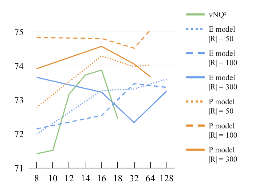
Figure 2: BLEU-4 scores on the ATP task. No constraint is placed. The horizontal axis represents $|\mathcal{N}|(=|\mathcal{P}|)$.

Next, we evaluate the models on the three hard transfer tasks from the StylePTB dataset Lyu et al. (2021) and a small-scale En-Fr machine translation dataset Lake and Baroni (2018). Tab. 2 shows results of the models with different constraints. Low-rank models generally achieve comparable or better performance and consume much less memory. We can also find that the soft tree hierarchy constraint outperforms hard constraints and is very helpful when it comes to extremely small data (i.e., AEM and VEM). The coverage constraint also improves performance in most cases.

5.3 Analysis

We study how the number of nonterminals affects performance. On our computer, we can use at most 18/64/128 nonterminals in vanilla Neural QCFG/the P model/the E model, showing that our low-rank models are more memory-friendly than vanilla Neural QCFG. We report results in Fig. 2. There is an overall trend of improved performance with more nonterminals (with some notable exceptions). When the numbers of nonterminals are the same, the P model outperforms vanilla Neural QCFG consistently, showing its superior parameter efficiency. In contrast, the E model is defeated by vanilla QCFG and the P model in many cases, showing the potential harm of separating $\alpha_{i},\alpha_{j},\alpha_{k}$.

5.4 Speed Comparison

We benchmark speed and memory usage using synthetic datasets with different sequence lengths. Fig. 3 and 4 illustrate the results. Compared to the standard Neural QCFG, the E model and P model are significantly faster and have a lower memory footprint. This enables them to model longer sequences effectively. For data construction and more results, please refer to Appx. D.3.

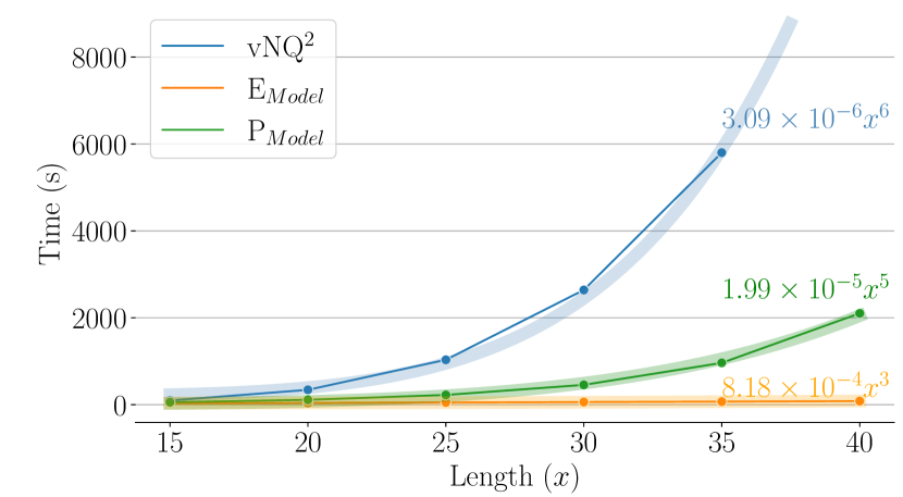
Figure 3: The duration required to train one epoch on synthetic datasets with different length ($x=S=T$). Thick and shallow lines are fitted curves based on time complexities of vNQ², E_Model and P_Model, i.e., $O(x^{6}),O(x^{3})$ and $O(x^{5})$.

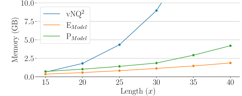
Figure 4: Memory usage for training with batch size 1 on synthetic datasets with different length ($x=S=T$).

6 Conclusion

We have presented two low-rank variants of Neural QCFG based on decomposition for efficiency and two new constraints over tree hierarchy and source coverage. Experiments on three datasets validate the effectiveness and efficiency of our proposed models and constraints.

7 Limitations

First, unlike decoders in neural seq2seq models, which can attend to any previously generated tokens, QCFGs have a strong context-free independence assumption during generation. With this assumption, Neural QCFG cannot model some complex distributions. A potential solution is to use stronger grammars, such as RNNG Dyer et al. (2016) and Transformer Grammars (TG; Sartran et al., 2022).

Second, we assume that both the grammars used by the source-side parser and QCFG are in CNF. Although it is convenient for discussion and implementation, CNF does not suit for modeling the structure of practical sequences. In semantic representations (e.g., Abstract Meaning Representation Banarescu et al. (2013)), a predicate could have more than two arguments. Ideally, we should represent $n$-ary predicates with $n$-ary rules. However, for grammars in CNF, $n-1$ unnatural binary rules are required to represent $n$-ary predicates. In natural language, we will face semantically meaningless spans due to CNF, which is discussed in Sec 4.2.

Third, although using decomposition improves the speed and the memory requirement, our low-rank models still cost much more computation resources than neural seq2seq models for two main reasons. (1) A large amount of nonterminal symbols increase the memory cost significantly. (2) Because finding the most probable string $t_{2}$ from $p_{\theta}(t_{2}|t_{1})$ is NP-hard Sima’an (1996); Lyngsø and Pedersen (2002), we follow Kim (2021) to use a decoding strategy with heavy sampling. For real data, we may need to sample hundreds or thousands of sequences and then rank them, which can be much slower than the decoding of neural seq2seq models.

Appendix A Time Complexity of P Model

Let $\beta_{ij},\beta_{jk}\in\mathbb{R}^{|\mathcal{N}|\times|t_{1}|}$ be two cells in the chart of the dynamic programming. $\beta_{ij}(x,y)$ denotes indexing into the matrix. Denote $A[\alpha_{1}]\rightarrow B[\alpha_{2}]C[\alpha_{3}]$ as $r_{b}$. The state transition equation is

$$\beta_{ik}(A,\alpha_{1})=\sum_{\begin{subarray}{c}j,B,C\\ \alpha_{2},\alpha_{3}\end{subarray}}p(r_{b})\beta_{ij}(B,\alpha_{2})\beta_{jk}(C,\alpha_{3}).$$

Let’s define following terms:

$$\tilde{\beta}_{ij}(R,\alpha_{2})=\sum_{B}p(R,\alpha_{2}\rightarrow B)\beta_{ij}(B,\alpha_{2})$$

$$\tilde{\beta}_{jk}(R,\alpha_{3})=\sum_{C}p(R,\alpha_{3}\rightarrow C)\beta_{ij}(C,\alpha_{3})$$

$$\hat{p}=p(A[\alpha_{1}]\rightarrow R)p(R,\alpha_{1}\rightarrow\alpha_{2},\alpha_{3})$$

Then the state transition equation can be reformulated as:

$$\beta_{ik}(A,\alpha_{1})=\sum_{R,\alpha_{2},\alpha_{3}}\hat{p}\underbrace{\sum_{j}\tilde{\beta}_{ij}(R,\alpha_{2})\tilde{\beta}_{jk}(R,\alpha_{3})}_{\hat{\beta}_{ik}},$$

where $\hat{\beta}_{ij}\in\mathbb{R}^{|\mathcal{R}|\times|t_{1}|\times|t_{1}|}$. We can compute $\tilde{\beta}_{ij}$ in $O((|\mathcal{N}|+|\mathcal{P}|)|\mathcal{R}|S)$ and cache it for composing $\hat{\beta}_{ij}$. Then $\hat{\beta}_{ik}$ can be computed in $O(|\mathcal{R}|S^{2}T)$. Finally, we can compute $\beta_{ik}$ in $O(|\mathcal{R}|S^{3}+|\mathcal{N}||\mathcal{R}|S)$ by sum out $\alpha_{2},\alpha_{3}$ first:

$$\beta_{ik}(A,\alpha_{1})=$$

$$\sum_{R}p(A[\alpha_{1}]\rightarrow R)\sum_{\alpha_{2},\alpha_{3}}p(R,\alpha_{1}\rightarrow\alpha_{2},\alpha_{3})\hat{\beta}_{ik}$$

So, summing terms of all the above steps and counting the iteration over $i,k$, we will get $O(|\mathcal{R}|S^{2}T^{3}+((2|\mathcal{N}|+|\mathcal{P}|)|\mathcal{R}|S+|\mathcal{R}|S^{3})T^{2})$.

Appendix B Neural Parameterization

We mainly follow Kim (2021) to parameterize the new decomposed rules. First, we add embeddings of terms on the same side together. For example, we do two additions $e_{lhs}=e_{R}+e_{\alpha_{i}}$ and $e_{rhs}=e_{\alpha_{j}}+e_{\alpha_{k}}$ for $R,\alpha_{i}\rightarrow\alpha_{j},\alpha_{k}$, where $e_{x}$ denotes the embedding of $x$. Note that we use the same feed-forward layer $f$ as Kim (2021) to obtain $e_{x}$ from some feature $h_{x}$. i.e. $e_{x}=f(h_{x})$. Then, we compute the inner products of embeddings obtained in the previous step as unnormalized scores. For example, $p(R,\alpha_{i}\rightarrow\alpha_{j},\alpha_{k})\propto\exp(e_{lhs}^{\top}e_{rhs})$.

Appendix C Posterior Regularization

The problem $\min_{q\in\mathcal{Q}}\mathbb{KL}(q(t_{2})||p(t_{2}|t_{1},s_{2}))$ has the optimal solution

$$q^{*}=\frac{1}{Z(\lambda^{*})}p(t_{2}|t_{1},s_{2})\exp\{-\lambda^{*}\phi(t_{2})\},$$

where

$$Z(\lambda^{*})=\sum_{t_{2}}p(t_{2}|s_{1},t_{1})\exp\{-\lambda^{*}\phi(t_{2})\}$$

and $\lambda^{*}$ is the solution of the dual problem:

$$\max_{\lambda\geq 0}-b\cdot\lambda-\log Z(\lambda)$$

We can reuse the inside algorithm to compute $Z(\lambda^{*})$ efficiently because our $\phi(t)$ can be factored as $p(t_{2}|t_{1},s_{2})$:

$$p(t_{2}|t_{1},s_{2}) =\prod_{r\in t_{2}}p_{\theta}(r)$$

$$\phi(t) =\sum_{r\in t_{2}}\phi(r,t_{1}),$$

where $\phi(r,t_{1})=1$ if $t_{1}$ is in the left-hand side of $r$ and $\phi(r,t_{1})=0$ otherwise. Then, the solution $q^{*}$ can be written as

$$q^{*}(t_{2})\propto\prod_{r\in t_{2}}p_{\theta}(r)\exp\{-\lambda\phi(r,t_{1})\}.$$

Recall that we define $\phi(t)$ to be the counts of source nodes being aligned by nodes in $t$. We can factor $\phi(t)$ in terms of $r$ because each target tree non-leaf node invokes exactly one rule and only occurs on the left-hand side of that rule. So, the sum over $r$ is equivalent to the sum over target tree nodes.

Appendix D Experiments

D.1 Experimental Details

We implement vNQ², the E model, and the P model using our own codebase. We inherit almost all hyperparameters of Kim (2021) and a basic constraint: the target tree leaves/non-leaf nodes can only be aligned to source tree leaves/non-leaf nodes, and especially, the target tree root can only be aligned to the source tree root. One major difference is that, in our experiments, we do not use early-stopping and run fixed optimization steps, which are much more than the value set in Kim (2021) (i.e., 15). It is because in preliminary experiments, we found that the task metric (e.g., BLEU) almost always get improved consistently with the process of training, while the lowest perplexity occurs typically at an early stage (which is the criteria of early-stopping in Kim (2021)), and computing task metric is very expensive for Neural QCFGs. We report metrics on test sets averaged over three runs on all datasets except for SCAN. As mentioned in the code of Kim (2021), we need to run several times to achieve good performance on SCAN. Therefore, we report the maximum accuracy in twenty runs.

SCAN Lake and Baroni (2018) is a diagnostic dataset containing translations from English commands to machine actions. We conduct experiments on four splits: We evaluate our models on four splits of the SCAN Lake and Baroni (2018) dataset: simple, add primitive (jump), add template (around right) and length. The latter three splits are designed for evaluating compositional generalization. Following Kim (2021), we set $|\mathcal{N}|=10,|\mathcal{P}|=1$.

StylePTB Lyu et al. (2021) is a text style tranfer dataset built based on Penn Treebank (PTB; Marcus et al., 1993). Following Kim (2021), we conduct experiments on three hard transfer tasks: textitactive to passive (2808 examples), adjective emphasis (696 examples) and verb emphasis (1201 examples). According to Tab. 2, we set $|\mathcal{N}|=|\mathcal{P}|=32,|\mathcal{R}|=100$ for the E model and set $|\mathcal{N}|=|\mathcal{P}|=64,|\mathcal{R}|=100$ for the P model.

En-Fr MT Lake and Baroni (2018) is a small-scale machine translation dataset. We use the same split as Kim (2021). The size of training/validate/test set is 6073/631/583. We set $|\mathcal{N}|=|\mathcal{P}|=32,|\mathcal{R}|=100$ for the E model and $|\mathcal{N}|=|\mathcal{P}|=32,|\mathcal{R}|=196$ for the P model.

D.2 Tune Hyperparameter

We tune hyperparameters according to metrics on validation sets, either manually or with the Bayesian Optimization and Hyperband (BOHB) search algorithm Falkner et al. (2018) built in the wandb library. First, we tune $|\mathcal{N}|$, $|\mathcal{P}|$, $|\mathcal{R}|$ and the learning rate of parameters for parameterizing QCFG. We freeze hyperparameters related to the source-side parser, the contextual encoder (i.e., LSTM), and the TreeLSTM Tai et al. (2015); Zhu et al. (2015). For the ATP task from StylePTB, we run the grid search to plot Fig. 2 and choose the best hyperparameters. For other tasks, we run about 20 trials according to BOHB for each manually set search range. Typically, the size of a search range is 256 (four choices for each tunable hyperparameter). Next, we tune the strength of the coverage constraint for all models by running with $\gamma=0.5,1,2$.

D.3 Speed and Memory Usage Comparison

Tab. 3 shows the time and memory usage on synthetic datasets. Each synthetic dataset contains 1000 pairs of random sequences with the same length sampled from a vocabulary with size 5000, i.e., $\{(s_{1},s_{2})_{1},\dots(s_{1},s_{2})_{1000}\},s_{1},s_{2}\in\Sigma^{v},|\Sigma|=5000$ where $v$ is the length. We set $|\mathcal{N}|=|\mathcal{P}|=8$ for vanilla Neural QCFG and $|\mathcal{N}|=|\mathcal{N}|=50,|\mathcal{R}|=200$ for others. We train models on a computer with an NVIDIA GeForce RTX3090. Note that we disable the copy mechanism in Kim (2021) because of its complicated effects on memory usage, such that the results differ from Fig. 2 (in which models enable the copy mechanism).

$v$	Approach	Constraint	Batch size	Time (s)	GPU Memory (GB)
10	vNQ2	nil	8	25.6	1.42
		+H1	8	25.5	1.43
		+H2	8	113.8	7.67
		+S	8	60.5	2.46
		+C	8	132.7	3.08
	EModel	nil	8	20.1	1.59
		+C	8	40.4	1.59
	PModel	nil	8	30.7	3.78
		+H1	8	31.3	3.79
		+H2	8	64.0	6.41
		+S	8	45.8	4.08
		+C	8	73.9	4.02
20	vNQ2	nil	8	341.2	14.49
		+H1	8	342.4	14.60
		+H2	1	$\approx$16539.4	14.13
		+S	2	$\approx$1734.4	8.93
		+C	2	$\approx$4657.1	12.24
	EModel	nil	8	40.0	4.58
		+C	4	173.4	14.48
	PModel	nil	8	111.3	8.25
		+H1	8	110.8	8.29
		+H2	4	452.3	9.83
		+S	8	269.8	18.76
		+C	4	643.5	18.20
40	vNQ2		1	$\times$	$\times$
	EModel	nil	8	82.5	14.95
		+C	8	177.0	14.95
	PModel	nil	4	$\approx$2102.7	16.78
		+H1	4	$\approx$2097.6	16.96
		+H2	1	$\times$	$\times$
		+S	2	$\approx$2729.3	10.63
		+C	1	$\times$	$\times$

Table 3: Time and memory usage on synthetic datasets. We report statistics with as large as possbile batch size (in $1,2,4,8$). $\times$ represents that we get an out-of-memory error even if we set batch size to 1. $\approx$ represents that the value is estimated using a small portion of the dataset.

References

- Bahdanau et al. (2019) Dzmitry Bahdanau, Shikhar Murty, Michael Noukhovitch, Thien Huu Nguyen, Harm de Vries, and Aaron Courville. 2019. Systematic generalization: What is required and can it be learned? In International Conference on Learning Representations.
- Banarescu et al. (2013) Laura Banarescu, Claire Bonial, Shu Cai, Madalina Georgescu, Kira Griffitt, Ulf Hermjakob, Kevin Knight, Philipp Koehn, Martha Palmer, and Nathan Schneider. 2013. Abstract Meaning Representation for sembanking. In Proceedings of the 7th Linguistic Annotation Workshop and Interoperability with Discourse, pages 178–186, Sofia, Bulgaria. Association for Computational Linguistics.
- Bos (2008) Johan Bos. 2008. Wide-coverage semantic analysis with Boxer. In Semantics in Text Processing. STEP 2008 Conference Proceedings, pages 277–286. College Publications.
- Buhai et al. (2020) Rares-Darius Buhai, Yoni Halpern, Yoon Kim, Andrej Risteski, and David Sontag. 2020. Empirical study of the benefits of overparameterization in learning latent variable models. In Proceedings of the 37th International Conference on Machine Learning, volume 119 of Proceedings of Machine Learning Research, pages 1211–1219. PMLR.
- Chang et al. (2008) Ming-Wei Chang, Lev Ratinov, Nicholas Rizzolo, and Dan Roth. 2008. Learning and inference with constraints. In Proceedings of the 23rd National Conference on Artificial Intelligence - Volume 3, AAAI’08, page 1513–1518. AAAI Press.
- Chiu et al. (2021) Justin Chiu, Yuntian Deng, and Alexander Rush. 2021. Low-rank constraints for fast inference in structured models. Advances in Neural Information Processing Systems, 34:2887–2898.
- Chiu and Rush (2020) Justin Chiu and Alexander Rush. 2020. Scaling hidden Markov language models. In Proceedings of the 2020 Conference on Empirical Methods in Natural Language Processing (EMNLP), pages 1341–1349, Online. Association for Computational Linguistics.
- Chomsky (1959) Noam Chomsky. 1959. On certain formal properties of grammars. Information and Control, 2(2):137–167.
- Cohen et al. (2013) Shay B. Cohen, Giorgio Satta, and Michael Collins. 2013. Approximate PCFG parsing using tensor decomposition. In Proceedings of the 2013 Conference of the North American Chapter of the Association for Computational Linguistics: Human Language Technologies, pages 487–496, Atlanta, Georgia. Association for Computational Linguistics.
- Devlin et al. (2019) Jacob Devlin, Ming-Wei Chang, Kenton Lee, and Kristina Toutanova. 2019. BERT: Pre-training of deep bidirectional transformers for language understanding. In Proceedings of the 2019 Conference of the North American Chapter of the Association for Computational Linguistics: Human Language Technologies, Volume 1 (Long and Short Papers), pages 4171–4186, Minneapolis, Minnesota. Association for Computational Linguistics.
- Dyer et al. (2016) Chris Dyer, Adhiguna Kuncoro, Miguel Ballesteros, and Noah A. Smith. 2016. Recurrent neural network grammars. In Proceedings of the 2016 Conference of the North American Chapter of the Association for Computational Linguistics: Human Language Technologies, pages 199–209, San Diego, California. Association for Computational Linguistics.
- Falkner et al. (2018) Stefan Falkner, Aaron Klein, and Frank Hutter. 2018. Bohb: Robust and efficient hyperparameter optimization at scale. In International Conference on Machine Learning.
- Frey (2002) Brendan J. Frey. 2002. Extending factor graphs so as to unify directed and undirected graphical models. In Proceedings of the Nineteenth Conference on Uncertainty in Artificial Intelligence, UAI’03, page 257–264, San Francisco, CA, USA. Morgan Kaufmann Publishers Inc.
- Ganchev et al. (2010) Kuzman Ganchev, João Graça, Jennifer Gillenwater, and Ben Taskar. 2010. Posterior regularization for structured latent variable models. J. Mach. Learn. Res., 11:2001–2049.
- Gehring et al. (2017) Jonas Gehring, Michael Auli, David Grangier, Denis Yarats, and Yann N Dauphin. 2017. Convolutional sequence to sequence learning. In International conference on machine learning, pages 1243–1252. PMLR.
- Herzig and Berant (2021) Jonathan Herzig and Jonathan Berant. 2021. Span-based semantic parsing for compositional generalization. In Proceedings of the 59th Annual Meeting of the Association for Computational Linguistics and the 11th International Joint Conference on Natural Language Processing (Volume 1: Long Papers), pages 908–921, Online. Association for Computational Linguistics.
- Kim (2021) Yoon Kim. 2021. Sequence-to-sequence learning with latent neural grammars. In Advances in Neural Information Processing Systems, volume 34, pages 26302–26317. Curran Associates, Inc.
- Koehn et al. (2007) Philipp Koehn, Hieu Hoang, Alexandra Birch, Chris Callison-Burch, Marcello Federico, Nicola Bertoldi, Brooke Cowan, Wade Shen, Christine Moran, Richard Zens, Chris Dyer, Ondřej Bojar, Alexandra Constantin, and Evan Herbst. 2007. Moses: Open source toolkit for statistical machine translation. In Proceedings of the 45th Annual Meeting of the Association for Computational Linguistics Companion Volume Proceedings of the Demo and Poster Sessions, pages 177–180, Prague, Czech Republic. Association for Computational Linguistics.
- Lake and Baroni (2018) Brenden Lake and Marco Baroni. 2018. Generalization without systematicity: On the compositional skills of sequence-to-sequence recurrent networks. In International conference on machine learning, pages 2873–2882. PMLR.
- Li et al. (2018) Yanyang Li, Tong Xiao, Yinqiao Li, Qiang Wang, Changming Xu, and Jingbo Zhu. 2018. A simple and effective approach to coverage-aware neural machine translation. In Proceedings of the 56th Annual Meeting of the Association for Computational Linguistics (Volume 2: Short Papers), pages 292–297, Melbourne, Australia. Association for Computational Linguistics.
- Loula et al. (2018) João Loula, Marco Baroni, and Brenden Lake. 2018. Rearranging the familiar: Testing compositional generalization in recurrent networks. In Proceedings of the 2018 EMNLP Workshop BlackboxNLP: Analyzing and Interpreting Neural Networks for NLP, pages 108–114, Brussels, Belgium. Association for Computational Linguistics.
- Lyngsø and Pedersen (2002) Rune B. Lyngsø and Christian N.S. Pedersen. 2002. The consensus string problem and the complexity of comparing hidden markov models. Journal of Computer and System Sciences, 65(3):545–569. Special Issue on Computational Biology 2002.
- Lyu et al. (2021) Yiwei Lyu, Paul Pu Liang, Hai Pham, Eduard Hovy, Barnabás Póczos, Ruslan Salakhutdinov, and Louis-Philippe Morency. 2021. StylePTB: A compositional benchmark for fine-grained controllable text style transfer. In Proceedings of the 2021 Conference of the North American Chapter of the Association for Computational Linguistics: Human Language Technologies, pages 2116–2138, Online. Association for Computational Linguistics.
- Mann and McCallum (2007) Gideon S. Mann and Andrew McCallum. 2007. Simple, robust, scalable semi-supervised learning via expectation regularization. In Proceedings of the 24th International Conference on Machine Learning, ICML ’07, page 593–600, New York, NY, USA. Association for Computing Machinery.
- Marcus et al. (1993) Mitchell P. Marcus, Beatrice Santorini, and Mary Ann Marcinkiewicz. 1993. Building a large annotated corpus of English: The Penn Treebank. Computational Linguistics, 19(2):313–330.
- Mnih et al. (2016) Volodymyr Mnih, Adrià Puigdomènech Badia, Mehdi Mirza, Alex Graves, Tim Harley, Timothy P. Lillicrap, David Silver, and Koray Kavukcuoglu. 2016. Asynchronous methods for deep reinforcement learning. In Proceedings of the 33rd International Conference on International Conference on Machine Learning - Volume 48, ICML’16, page 1928–1937. JMLR.org.
- Rabanser et al. (2017) Stephan Rabanser, Oleksandr Shchur, and Stephan Günnemann. 2017. Introduction to tensor decompositions and their applications in machine learning.
- Rush (2020) Alexander Rush. 2020. Torch-struct: Deep structured prediction library. In Proceedings of the 58th Annual Meeting of the Association for Computational Linguistics: System Demonstrations, pages 335–342, Online. Association for Computational Linguistics.
- Sartran et al. (2022) Laurent Sartran, Samuel Barrett, Adhiguna Kuncoro, Miloš Stanojević, Phil Blunsom, and Chris Dyer. 2022. Transformer Grammars: Augmenting Transformer Language Models with Syntactic Inductive Biases at Scale. Transactions of the Association for Computational Linguistics, 10:1423–1439.
- Sharma et al. (2017) Shikhar Sharma, Layla El Asri, Hannes Schulz, and Jeremie Zumer. 2017. Relevance of unsupervised metrics in task-oriented dialogue for evaluating natural language generation. CoRR, abs/1706.09799.
- Shaw et al. (2021) Peter Shaw, Ming-Wei Chang, Panupong Pasupat, and Kristina Toutanova. 2021. Compositional generalization and natural language variation: Can a semantic parsing approach handle both? In Proceedings of the 59th Annual Meeting of the Association for Computational Linguistics and the 11th International Joint Conference on Natural Language Processing (Volume 1: Long Papers), pages 922–938, Online. Association for Computational Linguistics.
- Sima’an (1996) Khalil Sima’an. 1996. Computational complexity of probabilistic disambiguation by means of tree-grammars. In COLING 1996 Volume 2: The 16th International Conference on Computational Linguistics.
- Smith and Eisner (2006) David Smith and Jason Eisner. 2006. Quasi-synchronous grammars: Alignment by soft projection of syntactic dependencies. In Proceedings on the Workshop on Statistical Machine Translation, pages 23–30, New York City. Association for Computational Linguistics.
- Sutskever et al. (2014) Ilya Sutskever, Oriol Vinyals, and Quoc V Le. 2014. Sequence to sequence learning with neural networks. Advances in neural information processing systems, 27.
- Tai et al. (2015) Kai Sheng Tai, Richard Socher, and Christopher D. Manning. 2015. Improved semantic representations from tree-structured long short-term memory networks. In Proceedings of the 53rd Annual Meeting of the Association for Computational Linguistics and the 7th International Joint Conference on Natural Language Processing (Volume 1: Long Papers), pages 1556–1566, Beijing, China. Association for Computational Linguistics.
- Tu et al. (2016) Zhaopeng Tu, Zhengdong Lu, Yang Liu, Xiaohua Liu, and Hang Li. 2016. Modeling coverage for neural machine translation. In Proceedings of the 54th Annual Meeting of the Association for Computational Linguistics (Volume 1: Long Papers), pages 76–85, Berlin, Germany. Association for Computational Linguistics.
- Wang et al. (2021) Bailin Wang, Mirella Lapata, and Ivan Titov. 2021. Structured reordering for modeling latent alignments in sequence transduction. In Thirty-Fifth Conference on Neural Information Processing Systems.
- Wang et al. (2022) Bailin Wang, Ivan Titov, Jacob Andreas, and Yoon Kim. 2022. Hierarchical phrase-based sequence-to-sequence learning. arXiv preprint arXiv:2211.07906.
- Williams and Peng (1991) Ronald J. Williams and Jing Peng. 1991. Function optimization using connectionist reinforcement learning algorithms. Connection Science, 3(3):241–268.
- Wong and Mooney (2006) Yuk Wah Wong and Raymond Mooney. 2006. Learning for semantic parsing with statistical machine translation. In Proceedings of the Human Language Technology Conference of the NAACL, Main Conference, pages 439–446, New York City, USA. Association for Computational Linguistics.
- Yang et al. (2022) Songlin Yang, Wei Liu, and Kewei Tu. 2022. Dynamic programming in rank space: Scaling structured inference with low-rank HMMs and PCFGs. In Proceedings of the 2022 Conference of the North American Chapter of the Association for Computational Linguistics: Human Language Technologies, pages 4797–4809, Seattle, United States. Association for Computational Linguistics.
- Yang et al. (2021) Songlin Yang, Yanpeng Zhao, and Kewei Tu. 2021. PCFGs can do better: Inducing probabilistic context-free grammars with many symbols. In Proceedings of the 2021 Conference of the North American Chapter of the Association for Computational Linguistics: Human Language Technologies, pages 1487–1498, Online. Association for Computational Linguistics.
- Zhu et al. (2015) Xiaodan Zhu, Parinaz Sobihani, and Hongyu Guo. 2015. Long short-term memory over recursive structures. In Proceedings of the 32nd International Conference on Machine Learning, volume 37 of Proceedings of Machine Learning Research, pages 1604–1612, Lille, France. PMLR.