Fast Search-By-Classification for Large-Scale Databases Using Index-Aware Decision Trees and Random Forests

Abstract.

The vast amounts of data collected in various domains pose great challenges to modern data exploration and analysis. To find “interesting” objects in large databases, users typically define a query using positive and negative example objects and train a classification model to identify the objects of interest in the entire data catalog. However, this approach requires a scan of all the data to apply the classification model to each instance in the data catalog, making this method prohibitively expensive to be employed in large-scale databases serving many users and queries interactively. In this work, we propose a novel framework for such search-by-classification scenarios that allows users to interactively search for target objects by specifying queries through a small set of positive and negative examples. Unlike previous approaches, our framework can rapidly answer such queries at low cost without scanning the entire database. Our framework is based on an index-aware construction scheme for decision trees and random forests that transforms the inference phase of these classification models into a set of range queries, which in turn can be efficiently executed by leveraging multidimensional indexing structures. Our experiments show that queries over large data catalogs with hundreds of millions of objects can be processed in a few seconds using a single server, compared to hours needed by classical scanning-based approaches.

PVLDB Reference Format:
PVLDB, 16(11): 2845 - 2857, 2023.
doi:10.14778/3611479.3611492

PVLDB Artifact Availability:
The source code, data, and/or other artifacts have been made available at %leave␣empty␣if␣no␣availability␣url␣should␣be␣sethttps://github.com/decisionbranches/decisionbranches.

1. Introduction

The data volumes produced and processed in many domains are massive. In remote sensing and astronomy, for instance, the amount of data is currently rising to a new level due to technical advancements in satellites and telescopes (Cheng et al., 2020; Li et al., 2016; Zhang and Zhao, 2015). In particular, the unprecedented pace of increase in spatial and temporal resolutions is leading to the assembly of large-scale surveys consisting of exabytes of valuable data, as it is the case for the data catalogs associated with the Sentinel missions operated by the European Space Agency (ESA) (Drusch et al., 2012) or the Large Synoptic Survey Telescope (Ivezić et al., 2019). A common task in these and other domains is the search for “interesting” objects (Weiss, 2004; Bailer-Jones et al., 2008; Metcalf et al., 2019) in such massive databases, i. e., objects of particular value for a specific application. For example, an astronomer might be interested in a special type of galaxy, while a data analyst in the energy sector might be interested in wind turbines visible in satellite imagery.

Figure 1. Traditional search-by-classification trains models for each query set, causing latency or high costs when scanning the entire database. Our framework leverages a co-design of indexes and models for efficient retrieval of positive instances, significantly reducing search time.

There are two prominent methodologies to address such search tasks from a technical perspective. The first one is based on nearest neighbor search, where a user query is specified via a query object, and objects similar to the query object are returned as query result (Keisler et al., 2019). These query scenarios are known under the guise of content-based (image) retrieval (Wan et al., 2014) and have led to popular search engines such as Google’s reverse image search or geospatial search engines (Keisler et al., 2019). In general, the corresponding user queries can be answered efficiently using index structures or approximation techniques (Bentley, 1975; Keivani and Sinha, 2018). However, the restriction of nearest neighbor queries to a single search item per query may lead to incomplete and inaccurate query results, as it is challenging to model the user’s intent based on a single query instance. This restriction is particularly problematic when it is necessary to identify all instances of an interesting object in a given database, such as finding all wind turbines in satellite imagery to estimate their quantity. In such scenarios, the use of nearest neighbor search methods may prove insufficient.

The second methodology is based on the application of machine learning models, in particular classification models such as decision trees. Such a search-by-classification approach involves using a (small) labeled data set containing both positive and negative instances. Based on this data set—which can be seen as a “user query”—a classification model is trained. During the inference phase, the entire database is scanned, and the trained model is applied to classify each object. Only the objects classified as belonging to the target class (e. g., class “special galaxy”) will be returned as the search result. As users can specify both types of objects—the ones the search should return and those it should not return—search-by-classification approaches can capture the user’s query intent more precisely and, hence, generally produce search results with higher quality compared to single-object queries (Branco et al., 2016; Cheng et al., 2020; Wang et al., 2019). However, despite its superiority, search engines serving many users cannot employ this approach since scanning the entire database per user query is too time-consuming and induces a high latency.

Figure 1 illustrates the concept of search-by-classification on a database of satellite imagery over which many user queries have to be executed. Here, a data analyst can specify both “interesting” objects, such as different wind turbines, as well as “non-interesting” examples, such as ships or chimneys, via a binary classification data set (left: red and black borders indicate positive and negative examples, respectively). A classification model (middle: yellow regions) is then trained using suitable features extracted from the data (for the sake of illustration, a two-dimensional feature space is shown; typically, more features are considered). The classification model is then applied to the entire database and the objects classified as “interesting” are returned to the user (right: yellow dashed border; false positives/negatives are possible). Note that each user query requires a new training and a new scan of the entire database (e. g., “User Query 2” induces a new model and different results). Although the training phase might not take much time for small query data sets (e. g., training a decision tree might take a tenth of a second or less), the inference phase generally requires scanning all the data for each incoming user query, which can become very time-consuming for large data catalogs, with each query taking hours or even more to complete. Hence, the search-by-classification strategy either implies high latency—i. e., a long time necessary to scan the entire database—or high costs—i. e., the costs caused by the parallelization of scans over a massively parallel infrastructure to reduce the latency. Note that a typical user query aims at finding a relatively small subset of “interesting” objects in the database, i. e., the answers sets are often very small compared with the totality of the objects (e. g., in a database of satellite imagery, only one out of one million image patches might show a wind turbine). Thus, we would ideally wish to devise a method with per-query costs that do not grow in proportion to the input database size.

Figure 2. Fast search-by-classification with an index-aware classifier and pre-built indexes. The classifier uses range queries on indexes for efficient inference and obtains target objects quickly via spatial lookups, bypassing data scans.

Contributions: In this work, we introduce a novel search-by-classification framework that allows us to return an answer set efficiently with low latency and at low cost by exploiting pre-built index structures, see Figure 2. More precisely, we propose a co-design of machine learning models and indexes for fast search-by-classification. As detailed in Section 3, a set of multidimensional index structures is built in an offline phase, where each index corresponds to a random subset of features (which are extracted from the data). These multidimensional indexes are constructed only once for the entire database and are independent of a particular user query. Afterwards, in the query processing phase, a new classification model is trained for each new user query, where the construction of this model is “index-aware”, i. e., during the construction, information about the indexes built in the offline phase is taken into account. Instead of scanning the entire data catalog, the instances being classified as positive (“Target Objects”) can then be efficiently retrieved via range queries, i. e., the inference phase is supported by means of fast lookups over the pre-built index structures. Hence, for a typical user query with a small answer set, one can quickly return all the desired instances with minimal computing resources, which is essential for interactive search engines. Of note, this paper primarily focuses on databases with infrequent changes. In summary, our main contributions are as follows:

1. We propose a novel search-by-classification framework, which resorts to a co-design of index structures and machine learning models. Users can formulate queries with positive and negative examples and the retrieval of target objects in large databases can be done in a few seconds instead of the hours that scanning-based approaches would typically need.

2. To realize this framework, we propose an “index-aware” construction scheme for decision trees and random forests. Our central idea involves the construction of decision-tree-like models based on low-dimensional feature subsets that match multidimensional index structures. More precisely, we build fragments of the trees following a novel bottom-up construction instead of the well-known and commonly applied top-down construction scheme. The resulting models exhibit two important properties: (a) the classification quality of the models created bottom-up is close to that of their original top-down counterparts, and (b) the set of database instances assigned to the positive class in the inference phase can be efficiently retrieved via range queries.

3. We provide a prototype of our search-by-classification framework, implemented in Python with Cython optimizations. We also implemented a graphical search engine on top of the prototype (accessible at https://web.rapid.earth).

4. We conduct an extensive experimental evaluation of our prototype, which includes a case study in the geospatial domain with more than a billion image patches, a detailed analysis of the involved parameters, and an extensive comparison with competing search strategies. The results show that our search-by-classification framework yields accuracy comparable with traditional search-by-classification schemes that repeatedly scan the entire database while returning the results in a fraction of the time needed by those methods.

2. Background

We consider search tasks with user queries consisting of positive and negative examples, see again “User Query 1” and “User Query 2” in Figure 1. That is, each user query gives rise to a binary classification task and a user query is provided in the form of a data set $T=\{(\mathbf{x}_{1},y_{1}),\ldots,(\mathbf{x}_{n},y_{n})\}\subset{\mathbb{R}}^{d}\times\mathcal{Y}$ with $\mathcal{Y}=\{0,1\}$, where a $(\mathbf{x}_{i},y_{i})$ with $y_{i}=1$ corresponds to a positive example (target class) and $y_{i}=0$ to a negative example. Here, $d$ corresponds to the number of features that are either given or that are extracted per instance. For instance, in the case of image data, a feature extractor can be applied to extract meaningful features, see again Figure 2.

2.1. Decision Trees and Tree Ensembles

Decision trees are simple yet powerful models and remain among the most popular methods in machine learning (Hastie et al., 2009; Breiman, 2001). Typically, decision trees are built recursively in a top-down manner, see Algorithm 1. The root of the tree to be built corresponds to a subset $S\subseteq T$ of the available data instances (e. g., a subset of the data sampled uniformly at random with replacement). During the recursive construction, the data are typically split into two subsets at each node, which form the basis for the recursive construction of two subtrees that are the children of that node. The recursion stops as soon as an associated subset is pure, which means that all the instances belong to the same class, or as soon as some other stopping criterion is fulfilled.

Algorithm 1 TopDownConstruct($S$, $\mu$)

0:  Set $S\subset{\mathbb{R}}^{d}\times\mathcal{Y}$ and $\mu\in\{1,\ldots,d\}$.

0:  Decision tree $\mathcal{T}$ built for $S$

1:  if $S$ is pure (or some other criterion fulfilled) then

2:     return leaf node

3:  end if

4:  $(i^{*},\theta^{*})=argmax_{i\in\{i_{1},\ldots,i_{\mu}\}\subseteq\{1,\ldots,d\},\theta}G_{i,\theta}(S)$

5:  $\mathcal{T}_{l}$ = TopDownConstruct($L_{i,\theta}$)

6:  $\mathcal{T}_{r}$ = TopDownConstruct($R_{i,\theta}$)

7:  Generate node storing the pair $(i^{*},\theta^{*})$ and pointers to its subtrees $\mathcal{T}_{l}$ and $\mathcal{T}_{r}$. Let $\mathcal{T}$ denote the resulting tree.

8:  return $\mathcal{T}$

Each internal node corresponds to a subset $S\subseteq T$ of instances, which is split via a splitting dimension $i\in\{i_{1},\ldots,i_{\mu}\}$ and an appropriately chosen threshold $\theta\in{\mathbb{R}}$, where $\mu\leq d$ is a user-defined parameter that determines the number of random features that are considered per split. Typically, one aims at maximizing the so-called information gain, defined as:

(1) $$G_{i,\theta}(S)=Q(S)-\frac{|L_{i,\theta}|}{|S|}Q(L_{i,\theta})-\frac{|R_{i,\theta}|}{|S|}Q(R_{i,\theta})$$

Here, $L_{i,\theta}=\{(\mathbf{x},y)\in\ S\,|\,x_{i}\leq\theta\}$ is the subset of $S$ containing the elements whose $i$-th feature is less or equal to the threshold $\theta$ and $R_{i,\theta}=\{(\mathbf{x},y)\in\ S\,|\,x_{i}>\theta\}$ the subset of $S$ containing the remaining instances. Maximizing the information gain corresponds to minimizing the (weighted) “impurities” of the two subsets above, which is typically quantified by an impurity measure $Q$ (Hastie et al., 2009; Breiman, 2001). For binary classification scenarios—on which we focus in this work—one typically resorts to the Gini index, which is defined as

(2) $$Q(S)=\sum_{c=0}^{1}p_{S}^{c}(1-p_{S}^{c}),$$

where $p_{S}^{c}$ corresponds to the fraction of points in $S$ belonging to class $c\in\{0,1\}$. Given a decision tree, the predicted class for a new data point $\mathbf{x}\in{\mathbb{R}}^{d}$ is obtained by traversing the tree from top to bottom and by resorting to the information stored in that particular leaf (e. g., dominant class of the training instances assigned to that leaf). To avoid overfitting, fully-grown decision trees are often pruned in a post-processing phase.

While decision trees often exhibit a good performance in practice, their quality can be typically improved by considering ensembles. Random forests are a prominent example of this class of techniques (Breiman, 2001). A random forest consists of a user-defined number $M$ of decision trees $\mathcal{T}_{1},\ldots,\mathcal{T}_{M}$, which are built independently from each other. To obtain different individual models, one can consider so-called bootstrap samples that are drawn uniformly at random (with replacement) from the data $T$, different subsets $\{i_{1},\ldots,i_{\mu}\}$ of features for each node split, and different (random) splitting thresholds. A prediction $h(\mathbf{x})$ for a new point $\mathbf{x}\in{\mathbb{R}}^{d}$ is then obtained by combining the individual predictions, that is

(3) $$h(\mathbf{x})=\mathcal{C}\left(h_{1}(\mathbf{x}),\ldots,h_{M}(\mathbf{x})\right),$$

where $\mathcal{C}:{\mathbb{R}}^{M}\rightarrow{\mathbb{R}}$ depends on the learning scenario. For classification scenarios, a common choice is the majority vote (Hastie et al., 2009; Breiman, 2001), i. e., $\mathcal{C}\left(h_{1}(\mathbf{x}),\ldots,h_{M}(\mathbf{x})\right)=\operatorname{argmax}_{c\in\mathcal{Y}}|\{i\,|\,h_{i}(\mathbf{x})=c\}|$. For standard random forests (Breiman, 2001), the optimal splitting threshold is computed as in Line 4 of Algorithm 1. A well-known alternative choice is to instead select a random threshold between the minimum and the maximum feature value, which yields so-called extremely randomized trees (Geurts et al., 2006). It is worth stressing that such potentially “suboptimal” thresholds often yield competitive if not superior tree ensembles.

2.2. Multidimensional Indexes

Our novel index-aware classifier transforms the inference phase of decision trees and random forests to a set of range queries in low-dimensional spaces. Such queries are efficiently supported by spatial index structures, such as k-d trees (Bentley, 1975), which are commonly used in the context of, e. g., database systems or nearest neighbor search (Gaede and Günther, 1998). We therefore briefly summarize a few important concepts behind these index structures that are necessary for this work.

For multidimensional data, a k-d tree is a popular choice to speed up range queries and nearest neighbor search (Bentley, 1975). A k-d tree is a balanced binary search tree that recursively partitions the search space into two half-spaces at each node. Given $N$ points in the $d$-dimensional Euclidean space, such a tree can be built in ${\mathcal{O}}(N\log N)$ time using linear-time median finding and occupies ${\mathcal{O}}(N)$ additional space (Bentley, 1975). The time complexity of orthogonal range queries with multidimensional axis-parallel boxes defining the regions of interest over a k-d tree can be upper-bounded, in the worst case, by ${\mathcal{O}}(dN^{1-\nicefrac{{1}}{{d}}}+q)$, where $q$ is the number of points returned (Lee and Wong, 1977). Hence, sublinear time is needed to answer such queries. In practice, a k-d tree exhibits good performance for small $d$, e. g., $d=3$, and can be constructed as to store data objects in external memory while the tree is kept in main memory (Bentley, 1979). Another popular index structure for multidimensional data is the so-called range tree, which, along with fractional cascading, enables queries to be answered in ${\mathcal{O}}(\log^{d-1}N+q)$ time at the cost of an increased construction time and space consumption of ${\mathcal{O}}(N\log^{d-1}N)$ (d. Berg et al., 2008).

Care must be exercised when employing index structures over high-dimensional data. In particular, the difference in distances of a point to its nearest and farthest points drops dramatically as $d$ is increased, making indexing less and less effective (Beyer et al., 1999). At dimensionality as low as $d=5$, this effect is already highly pronounced, while indexes are expected to be outperformed by a full scan of the data at $d$ values as low as 10 (Beyer et al., 1999).

2.3. Decision Trees and Range Queries

During the inference phase of a standard decision tree built for a classification data set, a new instance is classified as positive in case the tree traversal ends up in a leaf containing only or mostly positive instances (e. g., if the decision is based on majority vote).

Figure 3. A decision tree partitions instances for two features. Inference phase classifies all instances in the yellow boxes as ”positive.” Retrieving positive instances from a large database is achieved through two orthogonal range queries.

A simple yet crucial observation is that orthogonal range queries can be employed—namely, one range query per leaf of the tree that corresponds to the positive class—to obtain all instances in the database that would be classified as positive. Figure 3 illustrates this observation for $d=2$ features. Without any optimization, these range queries would necessitate a full scan of the database to determine if instances fall within the bounds of a positive leaf. Instead, given a corresponding index structure pre-built for the database, this would allow to rapidly return the desired instances per user query without the need of a full scan in case one is given a low-dimensional feature space (e. g., $d\leq 4$).

However, in practice, more than two features are typically needed in order to achieve a satisfactory classification performance, i. e., decision trees are usually based on splits in many dimensions (e. g., $d=100$). There are two simple but suboptimal ways to conduct the range queries for such high-dimensional feature spaces:

1. Complete feature space: A naive approach would be to build a single $d$-dimensional index and to conduct a range query for each positive leaf. However, as discussed in Section 2.2, conducting such range queries would generally not be efficient, i. e., the increase in dimensionality, in general, negates the benefits of index structures.

2. Restricted feature space: An alternative approach would be to consider only a small subset of the features (e. g., only 4 features) when constructing a decision tree, so that the underlying feature space can efficiently be indexed. However, as shown in our experiments, this variant leads to models exhibiting a worse classification quality, especially given classification tasks that require many features to be taken into account. Also, considering multiple such low-dimensional feature spaces and picking the one that leads to the best classification performance generally leads to significantly worse results compared to a construction based on all $d$ features.

Next, we show how to efficiently implement the search for target objects without sacrificing classification quality.

3. Efficient Search-by-Classification

We start by outlining the overall search-by-classification framework, prior to providing the details of the algorithmic building blocks.

3.1. Overall Framework

The framework is based on two phases, (1) an offline preprocessing phase and (2) a query processing phase, see again Figure 2.

1. Offline preprocessing: The offline preprocessing phase is only conducted once for the entire database to pre-build a set of index structures. First, the data are processed via a feature extractor that outputs a $d$-dimensional feature vector per instance. The features should capture general characteristics of the data and are not tailored to any specific query. Afterwards, $k$ index structures $\text{idx}_{1},\ldots,\text{idx}_{k}$ are built via an index builder. More precisely, $k$ random feature subsets $F_{1},\ldots,F_{k}\subset\{1,\ldots,d\}$ with $|F_{i}|=D$ for $i=1,\ldots,k$ are considered, where $1\leq D\leq d$ is some small constant (e. g., $D=4$). For each of these subsets $F_{i}$, a corresponding multidimensional index $\text{idx}_{i}$ is built. For instance, given $d=100$ features and $D=4$, $\text{idx}_{1}$ could be an index for the feature subset $F_{1}=\{17,51,60,80\}$, $\text{idx}_{2}$ an index for $F_{2}=\{11,45,49,99\}$, and so on.

2. Query processing: In the query processing phase, each user query is formulated via a binary classification data set. First, the feature extractor used in the offline preprocessing phase is also used to extract a feature vector for each instance of the data set. Next, an adapted version of a decision tree/random forest is built for the given data set. As detailed below, information about the indexes built in the offline preprocessing phase are considered during the construction of these classifiers (dashed lines in Figure 2) such that the database instances being classified as “positive” can be efficiently retrieved via orthogonal range queries, supported by a corresponding index structure (solid lines).

Note that, since $D$ is small, the index structures built in the offline preprocessing phase will support efficient range queries in the spaces defined by the feature subsets. Typically, quite many index structures have to be built for our approach (e. g., $k=100$ or more). Next, in Section 3.2, we provide the details of our novel construction scheme for decision trees and random forests used in the query processing phase. In a nutshell, we build fragments of the decision trees following a new bottom-up approach instead of the well-known and commonly applied top-down construction scheme. These decision branches allow for efficient retrieval of the desired instances from the database, as we will show in Section 3.3.

3.2. Decision Branches

Our approach is based on an alternative construction scheme for decision trees, which essentially (only) yields the bottom parts of decision trees, which we call decision branches. Each of the decision branches is associated with a $d$-dimensional box $B$, similar to a leaf of a decision tree. We define $B$ as $B=(l_{1},r_{1}]\times\cdots\times(l_{d},{r}_{d}]\subset{\overline{\mathbb{R}}}^{d}$ with ${\overline{\mathbb{R}}}={\mathbb{R}}\cup\{-\infty,+\infty\}$. If the dimension $i$ of a box $B$ is left- and right-bounded (i. e., $l_{i}>-\infty$ and $r_{i}<+\infty$), we call it bounded w.r.t. dimension $i$, whereas if it is left- or right-bounded (i. e., $l_{i}>-\infty$ or $r_{i}<+\infty$), we call it half-bounded w.r.t. dimension $i$; otherwise, we call it unbounded w.r.t. dimension $i$. Furthermore, we denote the number of half-bounded and bounded dimensions of a box $B$ by $n_{b}(B)$ and the number of unbounded dimensions by $n_{u}(B)$, respectively. For instance, in Figure 3, the first box $B_{1}$ is bounded w.r.t. the second dimension and unbounded w.r.t. the first dimension (i. e., $n_{b}(B_{1})=1$ and $n_{u}(B_{1})=1$), whereas the second box $B_{2}$ is half-bounded w.r.t. both dimensions (i. e., $n_{b}(B_{2})=2$ and $n_{u}(B_{2})=0$).

A crucial aspect of our approach is that each box $B$ associated with a decision branch will be bounded in a few dimensions only (e. g., $n_{b}(B)\leq 4$) and that it will contain “mostly” positive instances. Also, the union of all these boxes will cover all the positive instances of a given query data set. Finally, the construction of the branches and the boxes will be conducted in such a way that, for each box $B$, the bounded dimensions will correspond to one of the index structures that were built for the entire database in the offline preprocessing phase. This will allow to efficiently retrieve all the database instances belonging to the boxes.

The construction scheme detailed next is, hence, “index-aware” in the sense that the generation of the decision branches and associated boxes takes the index structures into account that were built in the offline preprocessing phase, see again Figure 2.

3.2.1. Constructing Decision Branches

Algorithm 2 DecisionBranches($T$, $F_{1},\ldots,F_{k}$, $p$, $\mu$)

0:  Data $T=\{(\mathbf{x}_{1},y_{1}),\ldots,(\mathbf{x}_{n},y_{n})\}\subset{\mathbb{R}}^{d}\times\{0,1\}$, $F_{1},\ldots,F_{k}\subset\{1,\ldots,d\}$ with $|F_{i}|=D$, $i=1,\ldots,k$, for some $1\leq D\leq d$, $1\leq p\leq k$, and $\mu\in\{1,\ldots,d\}$.

0:  Set $\mathcal{T}=\{\left(B_{1},\mathcal{B}_{1}\right),\ldots,\left(B_{l},\mathcal{B}_{l}\right)\}$ of $d$-dimensional boxes $B_{1},\ldots,B_{l}$ with $n_{b}(B_{i})\leq D$ for $i=1,\ldots,l$ along with associated decision branches $\mathcal{B}_{1},\ldots,\mathcal{B}_{l}$.

1:  $T_{0}\leftarrow\{(\mathbf{x},y)\in T|y=0\}$; $T_{1}\leftarrow\{(\mathbf{x},y)\in T|y=1\}$

2:  $\mathcal{T}\leftarrow\{\}$

3:  repeat

4:     Let $(\mathbf{x^{\prime}},y^{\prime})$ by any positive instance in $T_{1}$

5:     $g_{opt}\leftarrow 0$; $B_{opt}\leftarrow None$

6:     $\mathcal{F}=\{F_{i_{1}},\ldots,F_{i_{p}}\}\subseteq\{F_{1},\ldots,F_{k}\}$

7:     for each $F\in\mathcal{F}$ do

8:        $B,g\leftarrow\textsc{GreedyMaxGainBox}(T_{0}\cup T_{1},\mathbf{x^{\prime}},F)$

9:        if $g>g_{opt}$ then

10:           $g_{opt}\leftarrow g$; $B_{opt}\leftarrow B$

11:        end if

12:     end for

13:     $T_{1},R_{1}\leftarrow\textsc{RemoveInstances}(T_{1},B_{opt})$

14:     $T_{0},R_{0}\leftarrow\textsc{RemoveInstances}(T_{0},B_{opt})$

15:     $\mathcal{B}$ $\leftarrow$ TopDownConstruct($R_{0}\cup R_{1}$, $\mu$)

16:     $\mathcal{T}\leftarrow\mathcal{T}\cup\left(B_{opt},\mathcal{B}\right)$

17:  until $T_{1}$ is empty

18:  return $\mathcal{T}$

Our construction scheme for decision branches is implemented via the function DecisionBranches shown in Algorithm 2. Its input is composed of a training set $T$ (corresponding to a single user query), the $k$ feature subsets $F_{1},\ldots,F_{k}\subset\{1,\ldots,d\}$ mentioned above with $|F_{i}|=D\leq d$ for $i=1,\ldots,k$ and $1\leq D\leq d$, a number $1\leq p\leq k$ of feature subsets to be tested per iteration, and a constant $\mu\in\{1,\ldots,d\}$.

After initializing the two sets $T_{0}=\{(\mathbf{x},y)\in T|y=0\}$ and $T_{1}=\{(\mathbf{x},y)\in T|y=1\}$, the algorithm incrementally removes positive instances from $T_{1}$. For each such positive instance $(\mathbf{x}^{\prime},1)$, a $d$-dimensional box is found containing $\mathbf{x^{\prime}}$ and potentially more data points. This is achieved by considering a random subset $\mathcal{F}=\{F_{i_{1}},\ldots,F_{i_{p}}\}\subseteq\{F_{1},\ldots,F_{k}\}$ of the given feature subsets $F_{1},\ldots,F_{k}$ and by selecting the box $B_{opt}\subset{\overline{\mathbb{R}}}^{d}$ that maximizes an information gain computed via the function GreedyMaxGainBox (see below). Given the box $B_{opt}$, the function RemoveInstances removes all instances from $T_{0}$ and $T_{1}$ whose data points are contained in $B_{opt}$ (see Algorithm 4). The instances removed from $T_{0}$ and $T_{1}$ are collected in the sets $R_{0}$ and $R_{1}$, respectively, and are subsequently used as input for the function TopDownConstruct, which simply builds a classical decision tree for this subset in a top-down manner, yielding the decision branch $\mathcal{B}$ (which consists of a single node in case $R_{0}\cup R_{1}$ is pure). Both the box $B_{opt}$ and the decision branch $\mathcal{B}$ are added to the set $\mathcal{T}$, which forms the output of DecisionBranches after all iterations are done.

Each call of DecisionBranches returns a set of decision branches along with the associated boxes. In this context, $B$ is a $d$-dimensional box (with at most $D$ bounded dimensions) resulting from the bottom-up construction phase (Lines 4–14 in Algorithm 2), while $\mathcal{B}$ is a decision branch that corresponds to a small decision (sub-)tree (constructed in a top-down manner), which separates the subset $R_{0}\cup R_{1}$ of the training points contained in $B$ (Line 15 of Algorithm 2). Overall, the set of all decision branches corresponds to a standard decision tree built in a top-down manner for all data points. Note, however, that we do not build this complete decision tree, but only the decision branches. Some examples of decision branches are provided in Figure 5. Each decision branch $\mathcal{B}$ (lower part of a decision tree) in the figure corresponds to a feature space $F\in\mathcal{F}$ and can be seen as a branch of an overall decision tree (outlined in gray; not built). The bounding box $B$ associated with a given $\mathcal{B}$ is visualized as a dashed black rectangle. The leaves of the branches corresponding to the positive class are highlighted in yellow.

3.2.2. Maximum Gain Boxes

Algorithm 3 GreedyMaxGainBox($S$, $\mathbf{x}^{\prime}$, $F$)

0:  $S=\{(\mathbf{x}_{1},y_{1}),\ldots,(\mathbf{x}_{m},y_{m})\}\subset{\mathbb{R}}^{d}\times\{0,1\}$, $\mathbf{x}^{\prime}\in{\mathbb{R}}^{d}$, and $F\subset\{1,\ldots,d\}$ with $|F|=D$ for some $1\leq D\leq d$.

0:  Box $B\subset{\overline{\mathbb{R}}}^{d}$ with $n_{b}(B)\leq D$ and gain $g\in{\mathbb{R}}$.

1:  $F_{s}=(i_{1},\ldots,i_{D})\leftarrow\textsc{RandomSequence}(F)$

2:  $B\leftarrow$ InitialEmptyBox($\mathbf{x^{\prime}}$, $S$, $F_{s}$)

3:  for $j=1,\ldots,D$ do

4:     $B\leftarrow\textsc{ExpandBox}(\mathbf{x^{\prime}},S,B,i_{j})$

5:  end for

6:  $g\leftarrow\textsc{Gain}(S,B)$

7:  return $B,g$

The function GreedyMaxGainBox, shown in Algorithm 3, computes, for a given point $\mathbf{x^{\prime}}\in{\mathbb{R}}^{d}$, a subset $S\subseteq T$ of the training instances, and a feature subset $F\subset\{1,\ldots,d\}$, a $d$-dimensional box $B$ with $n_{b}(B)\leq D$ along with an associated gain $g\in{\mathbb{R}}$. In a first step, a fixed yet random feature index sequence $F_{s}$ is defined based on $F$. In a second step, the function InitialEmptyBox computes an initial box $B$ that only contains the point $\mathbf{x^{\prime}}$ (and possibly duplicates of $\mathbf{x^{\prime}}$) and heuristically covers as much empty space as possible in the dimensions specified by $F_{s}$ (see Section 3.4 for the implementation details).

Next, this box is expanded according to an information gain criterion defined below by iterating over the same feature index sequence $F_{s}$ and by applying the function ExpandBox, see Figure 4.

Algorithm 4 $\textsc{RemoveInstances}(T,B$)

0:  Data set $T=\{(\mathbf{x}_{1},y_{1}),\ldots,(\mathbf{x}_{m},y_{m})\}\subset{\mathbb{R}}^{d}\times\{0,1\}$ and $d$-dimensional box $B\subset{\overline{\mathbb{R}}}^{d}$

0:  Data sets $\overline{T}\subset{\mathbb{R}}^{d}\times\{0,1\}$ and $\overline{R}\subset{\mathbb{R}}^{d}\times\{0,1\}$

1:  $\overline{R}\leftarrow\{(\mathbf{x},y)\in T\mid\mathbf{x}\in B\}$

2:  $\overline{T}\leftarrow\{(\mathbf{x},y)\in T\mid\mathbf{x}\notin B\}$

3:  return  $\overline{T},\overline{R}$

More precisely, for each dimension $i_{j}$ in Line 4, both the left and right boundary of the current box $B$ are expanded w.r.t. dimension $i_{j}$. This is done by only considering the points of $\overline{S}\subset S$ that are contained in a box $\overline{B}$, which is the same box as $B$ except that the left and right boundary in dimension $i_{j}$ are set $-\infty$ and $+\infty$, respectively. To expand the left boundary in dimension $i_{j}$, the points $\mathbf{x}\in\overline{S}$ with $x_{i_{j}}<x^{\prime}_{i_{j}}$ are sorted in increasing order w.r.t. their distance $|x_{i_{j}}-x^{\prime}_{i_{j}}|$ to the point $\mathbf{x^{\prime}}$ in dimension $i_{j}$. Starting with $I=\{\mathbf{x^{\prime}}\}$, the sorted points are then processed incrementally and added to the set $I$. Let $O=S\backslash I$ be the set of remaining “outer” points. To decide if the left boundary should be expanded, we compute the gain $G(S)$ via:

(4) $$G(S)=Q(S)-\frac{|I|}{|S|}Q(I)-\frac{|O|}{|S|}Q(O)$$

As for decision trees, $Q$ is a classification impurity measure such as the Gini index. After all or a pre-defined number $p_{m}$ of points (e. g., $p_{m}=20$) have been processed, the new left boundary $l_{i_{j}}$ of $B$ in dimension $i_{j}$ is set to the value so that the gain $G(S)$ is maximized. The right boundary $r_{i_{j}}$ of $B$ is computed similarly. The expansion is repeated for $j=1,\ldots,D$. In Figure 4, the overall process is visualized for the case of $D=2$.

(a) Initial Box

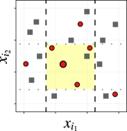
(b) $i_{1}$

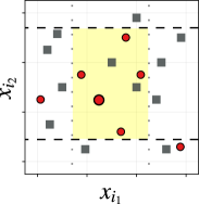
(c) $i_{2}$

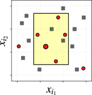
(d) Final Box

Figure 4. ExpandBox: The red points depict positive and the black points negative instances, respectively. The initially covered point corresponds to the positive instance $\mathbf{x}$.

Overall, the goal of ExpandBox is to expand the initial box in such a way that information gain is maximized (similarly to top-down construction of decision trees). At the end of Algorithm 3, the function Gain is used to compute the final gain induced by the “split” of $S$ into $I=S\cap B$ and $O=S\backslash I$. Both the final box $B$ as well as the final gain $g$ are returned by GreedyMaxGainBox.

3.2.3. Comparison with Decision Trees

Our construction scheme is hypothesized to produce fragments of standard decision trees, as they share common characteristics such as orthogonal splits, splits respecting infinity, and training based on an impurity criterion. In principle, these models could be generated via a top-down approach, which suggests that they belong to the same model space and are expected to achieve comparable generalization (confirmed empirically in Section 4.3.2). Yet, each box along with its associated decision branch only resort to a few features, which will enable fast spatial look-ups in the database. Also note that, for each positive instance, a large set of $k$ feature subsets is considered to identify an appropriate box containing mostly positive instances, which is motivated by the observation that, when constructing normal decision trees, care must (only) be taken when constructing the lower parts of the trees (i. e., essentially, arbitrary splits can be made in the top parts of trees, whereas discriminative feature splits are needed for the lower parts) (Gieseke and Igel, 2018).

3.2.4. Decision Branch Ensembles

The bottom-up construction scheme for the decision branches is driven by introducing randomness in various phases. For instance, a random sequence $F_{s}$ is defined based on $F$ in GreedyMaxGainBox. While this use of randomness is not strictly needed for single calls to DecisionBranches, it is crucial when generating ensembles of decision branches, as is the case for standard tree ensembles such as random forests and extremely randomized trees. Based on this observation, deriving an ensemble consisting of decision branch models is then straightforward and can be done by simply combining the sets $\mathcal{T}_{1},\ldots,\mathcal{T}_{M}$ obtained by $M$ calls of DecisionBranches, where only the instances of the database are returned that are classified as positive by the majority of the models.

3.3. Fast Query Processing

Figure 5. Answering user queries via decision branches and index structures pre-built for large databases.

The remaining task is efficient inferencing via range queries (Figure 2). Overall, we aim at processing many user queries with small latencies given a large database. In addition, we assume limited computational resources; in particular, our approach does not rely on the use of many servers. As mentioned above, we begin by pre-building a large number of index structures $idx_{1},\ldots,idx_{k}$ in the offline preprocessing phase. Note again that these indexes have to be built only once beforehand and are independent of a particular user query. The processing of a new user query, i. e., for a new data set $T=\{(\mathbf{x}_{1},y_{1}),\ldots,(\mathbf{x}_{n},y_{n})\}\subset{\mathbb{R}}^{d}\times\{0,1\}$ consisting of a few positive and many negative instances, then proceeds as follows:

1. In the first step, a set of decision branches (corresponding to a decision tree) is built via the function DecisionBranches.

2. In the second step, we conduct, for each decision branch $\mathcal{B}$ with associated box $B$ and feature subset $F$, an orthogonal range query using the index structure built beforehand for $F$ to retrieve all instances of the database contained in $B$.

3. Finally, in the third step, these instances are classified into positive or negative by the corresponding decision branches, where only positive instances are returned to the user.

Note that a crucial ingredient for the efficiency of our query processing is that each resulting box $B\subset{\mathbb{R}}^{d}$ associated with a decision branch is only (half-)bounded in a few dimensions, i. e., $n_{b}(B)\leq D$, where $D$ is a small constant (e. g., $D=4$). This property stems from the fact that such boxes are constrained using only the features provided by a set $F\subset\{1,\ldots,d\}$ with $|F|=D$, see again Algorithm 3. Thus, the index that is available for that feature subset $F$ can be used to efficiently conduct the corresponding range query.

The workflow is illustrated in Figure 5. To sum up, for each user query given as a classification data set, a set of decision branches is constructed. Each decision branch corresponds to a box (black dashed rectangles), and the database instances being contained in one of the boxes can quickly be retrieved using the associated index. The resulting (small) answer sets are then filtered for positive instances via the corresponding decision branch for each box.

3.4. Implementation Details

Here we provide some details related to InitialEmptyBox and TopDownConstruct used in Algorithm 2, as well as to the memory layout and space consumption of the index structures.

3.4.1. Initial Box

For the sake of completeness, we provide details related to the function InitialEmptyBox. For a given point $\mathbf{x^{\prime}}\in{\mathbb{R}}^{d}$, a subset $S$ of training instances, and a sequence $F_{s}=(i_{1},\ldots,i_{D})$, the procedure InitialEmptyBox constructs a $d$-dimensional box $B$ that only contains the query point $\mathbf{x^{\prime}}$ and no other points. At the same time, this box also covers as much empty space as possible in the dimensions specified by $F_{s}$. The box is computed by deriving bounds for the dimensions specified by $F_{s}$; the left and right bounds for the other dimensions are set to $-\infty$ and $+\infty$, respectively. Identifying such a box is known to be computationally challenging, even for low-dimensional spaces.

(a) Start

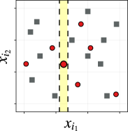
(b) $i_{1}$

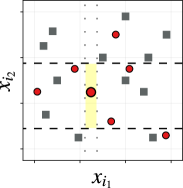
(c) $i_{2}$

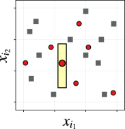
(d) Box

Figure 6. Illustration of InitialEmptyBox.

3.4.2. Decision Branch Models

In case $R_{0}\cup R_{1}$ is pure, TopDownConstruct in Algorithm 2 returns a single node. Given an impure set in $B_{opt}$ (see, e. g., Figure 4d), the procedure TopDownConstruct builds a tree $\mathcal{B}$ for the instances given in $R_{0}\cup R_{1}$. In our experiments, we consider two versions to implement this function. The first one, T_a, resorts to all $d$ features. The second one, T_s, only considers the $D$ features specified by the feature subset $F$ that corresponds to the box $B_{opt}$ (i. e., $\mathcal{B}\subset B_{opt}$ holds true). The benefit of the first implementation is that it generally yields slightly better models in terms of classification accuracy. However, it requires retrieving the full set of $d$ features returned by the range query. The benefit of the second approach is that the $D$ features can directly be stored in the leaves of the index structures (using ${\mathcal{O}}(ND)$ additional space), which, in turn, allows for immediate retrieval of the features needed when processing the range queries. However, this variant generally yields slightly worse classification results than T_a, see Section 4.

3.4.3. Hybrid Memory K-D Trees

A large number $k$ of index structures have to be pre-built for a large database. For k-d trees, ${\mathcal{O}}(N)$ additional space is needed, where $N$ is the number of elements in the database. Hence, given a large $k$, it might not be feasible to keep all these index structures in the main memory of a system. In order to address this problem, we implement an efficient k-d tree-based index that supports multidimensional range queries and leverages disk storage. In particular, our k-d tree implementation only stores the tree structure up to the leaves in main memory. The leaves containing the instances with all their features are stored consecutively on disk. If a query is now forwarded to the index structure, only the leaves that intersect with the query rectangle need to be loaded from disk. A crucial hyperparameter for the success of our k-d tree index is the leaf size. The smaller the size of the leaves, the less data not contained in the query rectangle is falsely loaded. Since the bottleneck of this method will tend to be the data loading time from disk, it can be expected that a smaller leaf size leads to faster query times. On the other hand, the loading time is also influenced by the block size of the underlying (file) system: leaves that are smaller than the actual block size cannot make proper use of device bandwidth. Additionally, the larger the leaf size, the smaller are the parts of the k-d trees that have to be kept in main memory. Ultimately, we meet a trade-off among all of these factors, making the optimal leaf size a critical hyperparameter that has to be determined before constructing the indexes. As we will show in our experiments, it is possible to keep the top parts of k-d trees in main memory for a large number k of index structures.

4. Experiments

Table 1. Summary of model notation.

Parameter	Description
B	Bottom-up (depth of $\mathcal{B}$ is 0)
Ts	Bottom-up + top-down (using $D$ features)
Ta	Bottom-up + top-down (using all $d$ features)
¡num¿t	DBEns: number of estimators (default: 25t)
¡num¿	DBranch/DBEns: D (default: 10)
¡num¿	DTree/RForest: # of features used (default: all)

We provide an extensive evaluation of our approach w.r.t. three aspects: (1) efficiency of index-supported decision branches and ensembles in terms of inference runtime against scan-based evaluation of decision trees and random forests as well as nearest neighbor search (Section 4.2); (2) sensitivity of decision branches models to crucial hyperparameters and comparison to traditional tree-based algorithms in (imbalanced) binary classification tasks (Section 4.3); and (3) trade-off between storage consumption of the underlying index structures and performance (Section 4.4). In particular, we consider a realistic case study with more than a billion data points. The results show that our search-by-classification framework yields as accurate results as traditional search-by-classification schemes (that have to scan the entire database per user query), albeit at dramatically reduced query processing times.

4.1. Experimental Setup

All experiments were conducted on an Ubuntu 18.04 server with 24 AMD EPYC 7402P cores, 192 GB DDR4-RAM and 30 TB of NVMe storage. The construction schemes for decision branches and for the hybrid memory k-d tree were implemented in Python 3.8, where Cython was used for computationally intensive parts.

4.1.1. Models

We consider the Scikit-Learn (Pedregosa et al., 2011) implementations of decision trees (DTree), random forests (RForest), and extremely randomized trees (ExTrees) as baseline search-by-classification models (which retrieve the positive instances by scanning the entire database). These models are compared with our novel decision branch approach (DBranch) as well as with a corresponding ensemble variant (DBEns) introduced in Section 3.2.4. For both DBranch and DBEns, three versions are considered. For the first version (B), TopDownConstruct returns a single node, i. e., all the decision branch models have depth zero. The other two versions, T_s and T_a, are described in Section 3.4.2. For T_s, TopDownConstruct only uses the features $F\in\mathcal{F}$ that yielded the box $B_{opt}$ (see Algorithm 2). In contrast, TopDownConstruct resorts all the $d$ features for T_a.

An overview of the notation is provided in Table 1. In our evaluation, we aim to demonstrate that our decision tree and tree ensemble variants yield a competitive classification performance compared to the aforementioned baselines, without the need to scan the entire data catalog. Additionally, we include an efficient exact nearest neighbor search baseline (denoted by NNB) for comparison, which uses our k-d tree implementation (Bentley, 1979) to accelerate the search. This baseline indicates the classification performance that users would experience when interacting with an NN-based search engine that only allows single-instance search queries, an approach commonly found in visual search engines (Keisler et al., 2019). To establish a fair comparison, we treat the NNB as a model, where all $\mathcal{K}$ nearest neighbors produced given a user query are considered to be positive, while all other instances are considered to be negative. We assess its classification performance as an average among all single-instance searches obtained from the positive instances in a training set, thus abstracting a notion of typical result quality.

4.1.2. Metrics

We assess the quality of the models using the $F_{1}$-score, defined as the harmonic mean of precision ${\mathcal{P}}$ and recall ${\mathcal{R}}$, i. e., $F_{1}=2\cdot\nicefrac{{{\mathcal{P}}\cdot{\mathcal{R}}}}{{({\mathcal{P}}+{\mathcal{R}}}})$. The application-level impact of a high $F_{1}$-score (e. g., ~0.8) is achieving a good trade-off between precision and recall, where the system misses only a few relevant objects during the search. In addition to measuring the total execution time $T_{total}$ for the approaches, we also measure the training time $T_{train}$ and the query time $T_{query}$ for the different models, where the former captures the time needed to build the classification models and the latter to retrieve instances from the database.

4.2. Efficiency Study of Index-Aware Models

(a) Chimney

(b) Plane

(c) Ship

(d) PV Panel

(e) Tank

(f) Turbine

Figure 7. Aerial Data Set

We begin by demonstrating the effectiveness of our approach through a geospatial case study, using 12.5 cm per pixel resolution aerial imagery of Denmark from 2018 (non-public data set). The images are decomposed into 256×256 pixel patches, resulting in a data set size of $N=1,441,557,000$ patches. We identified and manually collected labels for six classes of potentially interesting objects, namely chimneys, planes, ships, PV panels, storage tanks, and (wind) turbines, see Figure 7. Feature extraction was performed via a ResNet101 neural network (He et al., 2016) pretrained on ImageNet (Russakovsky et al., 2015), where the feature embedding layer was adapted to yield $d=50$ features. The model weights were fine-tuned by training the network for a few epochs using labeled patches over 7 classes (i. e., those depicted in Figure 7 and an additional class for “other objects”) and the Adam optimizer (Kingma and Ba, 2015) with a learning rate of $0.0001$. Note that the ResNet101 was used only as a pre-processing step, since its application would have required scanning the complete data set for every user query.

To generate realistic queries, we considered, for each user query, a set of $30$ “rare” patches ($y=1$) belonging to the target class (e. g., PV panels). We also utilized $30,000$ “non-rare” patches ($y=0$) for each query, which were selected uniformly at random from the catalog (containing $N$ patches). This approach can be justified by (a) the assumption that non-rare patches are extremely more frequent than rare ones for the search tasks addressed (e. g., only about one out of one hundred thousand patches corresponds to a PV panel, which leads to only a few falsely labeled instances in our user query) and by (b) that a user query in practice might also contain a few falsely labeled instances (e. g., non-rare patches labeled as rare).

4.2.1. Query Response Time and Classification Quality.

We compare the average total time $T_{total}$ of user queries induced by the six classes shown in Figure 7. As detailed above, each query was composed of $30,030$ training instances. The quality in terms of $F_{1}$-score was computed using a hold-out set consisting of $110,000$ labeled instances, whereas the runtime results were obtained using the entire database with $N$ instances. We repeated the experiment five times with different seeds (accounting for randomness) and report averaged runtimes and scores.

The k-d tree indexes were built for $D=3$ and different values for $k\in\{50,150,300\}$ with a fixed leaf size of $5,632$. To implement a fast NNB, we built another k-d tree using all the $N$ instances in the database and three (random) features. The leaf size was set to 43 and the full tree was loaded into memory (including the leaves). We measured the query time for NNB by searching for the $\mathcal{K}=1,000$ nearest neighbors of $100$ labeled interesting data instances and report the average query times. The $F_{1}$-score was obtained via the hold-out set of $110,000$ labeled instances, where for each user query instance, $\mathcal{K}$ was set to the (true) number of positive instances in the entire database.

Table 2 summarizes the results obtained. For $k=300$ (right column), the fastest DBranch model (DBranch _[B,3]) achieved a 715$\times$ lower $T_{total}$ than the DTree model, while exhibiting a comparable $F_{1}$-score. In the ensemble case, ensembles with of 5 and 25 decision branch models were considered, respectively. Here, the fastest DBEns model (DBEns _[Ts,5t,3]) achieved a 195$\times$ lower $T_{total}$ than the RForest (25 trees) and ExTrees (25 trees) with a similar $F_{1}$-score. The NNB was substantially faster than the other approaches, yielded, however, a significantly worse $F_{1}$-score. The table also provides insights w.r.t. space consumption and model quality. Specifically, 600 GB of disk storage were required to store the entire database, while the k-d tree indexes required 13 TB of additional storage for $k=300$ (to store the associated leaves). These storage requirements could be reduced at a minor expense in $F_{1}$-score by selecting a lower value of $k$ (e. g., 50 or 150), see again Table 2.

Table 2. Results on aerial image data set (size 0.6 TB). Time in seconds. Index size is reported next to each value of $k$.

Model	$k=50\rightarrow 2.17$ TB				$k=150\rightarrow 6.5$ TB				$k=300\rightarrow 13$ TB
	$T_{train}$	$T_{query}$	$T_{total}$	$F_{1}$-score	$T_{train}$	$T_{query}$	$T_{total}$	$F_{1}$-score	$T_{train}$	$T_{query}$	$T_{total}$	$F_{1}$-score
DBranch [B,3]	0.307	1.556	1.863	0.800	0.398	1.047	1.445	0.833	0.583	0.971	1.554	0.850
DBranch [Ts,3]	0.310	1.445	1.756	0.801	0.399	1.090	1.489	0.824	0.567	0.892	1.459	0.847
DBranch [Ta,3]	0.335	16.618	16.953	0.818	0.420	14.685	15.105	0.833	0.672	13.844	14.516	0.854
DTree	0.855	1,043.433	1,044.288	0.829	0.855	1,043.433	1,044.288	0.829	0.855	1,043.433	1,044.288	0.829
NNB	—	0.298	0.298	0.431	—	0.298	0.298	0.431	—	0.298	0.298	0.431
DBEns [B,5t,3]	0.529	9.760	10.288	0.895	0.993	5.666	6.658	0.914	1.862	5.156	7.018	0.912
DBEns [Ts,5t,3]	0.508	8.418	8.926	0.884	1.013	5.455	6.468	0.904	1.886	4.895	6.780	0.904
DBEns [B,25t,3]	0.891	28.607	29.497	0.915	1.543	22.639	24.182	0.925	2.729	19.716	22.445	0.930
DBEns [Ts,25t,3]	0.892	26.466	27.358	0.897	1.573	21.212	22.785	0.916	2.688	18.596	21.284	0.921
RForest	0.274	1,319.688	1,319.961	0.904	0.274	1,319.688	1,319.961	0.904	0.274	1,319.688	1,319.961	0.904
ExTrees	0.122	1,332.026	1,332.148	0.950	0.122	1,332.026	1,332.148	0.950	0.122	1,332.026	1,332.148	0.950

4.2.2. Optimal $k$-d Tree Leaf Size

Next, we investigate the influence of the leaf size of our k-d trees by considering k-d trees with varying leaf sizes. This experiment was conducted for two feature subset sizes, $D=3$ and $D=6$, and for each of the two cases, $k=10$ random feature subsets were considered. For each of these feature subsets, k-d trees with leaf sizes ranging from 22 to 22,582 were built. For each of the six classes shown in Figure 7, one user query was generated, each with 30 positive and 30,000 negative instances. Fitting a decision branch model for each such query led to a set of range queries (i. e., the $B_{opt}$ boxes), which were processed by a corresponding k-d tree index. To assess the impact of the leaf sizes on the query time, we report the average query time needed to process such user queries for each case and for each leaf size. We repeated the experiments for two settings, which we call “cold” and “warm”. For the cold setting, underlying caches (e. g. disk, OS) were emptied, whereas for the warm setting the loaded objects of a query were already cached, which led to a reduced loading time. We report results for both settings in Figure 8. The minimal query time for the cold setting was achieved with a leaf size of $5,632$. Note that $T_{query}$ was slightly larger for $D=6$, which is in line with the runtime bounds and performance issues in high-dimensional spaces of index structures summarized in Section 2, i. e., longer query times for growing $D$. For the warm setting, the query times were significantly reduced. This behavior suggests that, if redundant boxes occur during the search, smaller leaf sizes may be considered to make better use of caching opportunities. Figure 8 also shows the memory footprint of a single k-d tree index structure for different leaf sizes and $D$. As expected, memory requirements are inversely proportional to leaf size. Hence, when halving the leaf size, memory requirements double due to the larger tree that needs to be loaded into memory (the leaves are stored on disk).

Figure 8. Impact of leaf size on query time and size of a single k-d tree. No results for $D=6$ and leaf size 22 due to exceeding machine memory capacity.

For the runtime evaluation provided below, we therefore selected the optimal leaf size of $5,632$, since it not only achieved the fastest query time but also exhibited a small memory footprint. The latter allows for loading hundreds of index structures in memory at once, even on commodity hardware. More specifically, one index requires only 24 MB for $D=3$ and 48 MB for $D=6$.

4.2.3. Scaling Behavior of $k$-d Tree.

Next, we analyze if the theoretical time complexity ${\mathcal{O}}(dN^{1-\nicefrac{{1}}{{d}}}+q)$ of range queries over a k-d tree can be achieved in practice with our implementation. To do so, we measured the query time $T_{query}$ of the k-d tree for increasing sizes of $N$. We stopped the search after 10 leaves had been visited to keep $q$ (number of points returned) at a constant level. Thereby, the focus was on the tree traversal time instead of the time needed to return the contained data instances. In our analysis, we built k-d tree indexes for different subset sizes $N$ and $D=3$, scaled the number of instances by selecting instances at random from the database, and report the query times averaged over five runs. To measure those query times, we generated 300 random boxes ensuring no overlap, so as to minimize the chance of caching when leaves were loaded multiple times. Figure 9 (left) shows that the scaling behavior of our k-d tree implementation falls in-between the asymptotic curves for ${\mathcal{O}}(logN)$ and ${\mathcal{O}}(N^{1-1/3})$, which, again, is in line with the runtime bounds provided in Section 2.

Figure 9. Scaling behavior of our k-d tree search for $D=3$ (left) and traditional tree-based methods.

4.2.4. Scaling Behavior of Decision Branches.

Finally, we assessed the scaling behavior of the two search-by-classification models with the lowest $T_{total}$ in Table 2 for $k=300$. Figure 9 (right) shows the behavior of the models as we increased the number of points $N$ in the data set. Note that, similarly to the k-d tree experiments above, data instances were selected at random for each value of $N$. Each measurement for DBranch _[Ts,3] was averaged over three repetitions with different seeds to account for randomness in the method, while a single repetition was used for the DTree. DBranch _[Ts,3] exhibits very slow growth in $T_{total}$ (e. g., almost no increase for the last three measurements). By contrast, $T_{total}$ for DTree grows as expected, linearly with $N$. When $N>10^{9}$, DBranch _[Ts,3] outperforms DTree by almost three orders of magnitude, yielding the query results in a few seconds only.

To conclude, our search framework enables quick processing of such user queries (e. g., search for planes in satellite imagery) and can report the (complete) answer set per query in a few seconds only, compared to minutes needed by scanning-based approaches. It is worth stressing that the runtime benefits will become more and more prominent and important in case the database would contain even more instances (e. g., hundreds of billions of instances).

4.3. Sensitivity Analysis and Benchmark

Table 3. Data Sets

Data set	$\bar{n}$	$d$	$K$
iris	150	4	3
satimage	6,430	36	6
letter	20,000	16	26
mnist	60,000	784	10
senseit	98,528	100	3
covtype	581,012	54	7

Next, we consider six more data sets listed in Table 3 with $d$ features, $K$ classes, and $\bar{n}$ instances. Most of them are widely used for comparing binary classification models. However, our setup differs from known benchmarks in order to mimic a use case similar to a search engine for imbalanced data. To resemble such a case, we converted the original classification tasks to binary “one-vs-all” problems. That is, for each data set, we selected a class $c_{p}$ to represent the positive class, while the remaining ones were regarded as negative. We fixed the number of positive objects in the training set to $30$ and picked $\left(\nicefrac{{30}}{{\bar{n}_{c_{p}}}}\right)\cdot\bar{n}_{c_{n}}$ instances from each other class $c_{n}$, where $\bar{n}_{c_{p}}$ and $\bar{n}_{c_{n}}$ were the number of instances belonging to the positive class $c_{p}$ and the other class $c_{n}$, respectively. The remaining instances were split up to form (almost) equal-sized validation and test sets. The hyperparameters of each model were optimized via grid search on the validation set and the final model qualities were assessed using the test set. Each run was repeated three times with different (random) seeds.

4.3.1. Influence of Parameters

The sensitivity of the different decision branch variants w.r.t. the feature subset size $D$ and the number of feature subsets $p$ tested is shown in Figure 10. The results for $F_{1}$-scores are averaged across all one-vs-all classification tasks and data sets, while the training time results are shown for covtype only (since this data set is dominant in terms of number of data instances, and, hence, runtime). We observe that all models benefit from larger $D$, while $F_{1}$-scores increase only slightly beyond $D=6$. The $T_{a}$ model variants (i. e., including both bottom-up and top-down constructions using all available features) are less dependent on large $D$ while exhibiting comparable training time to $T_{s}$ variants (i. e., including subsets of $D$ features only). This effect indicates that $T_{a}$ variants can more effectively compensate for suboptimal boxes learned during the bottom-up construction phase by a subsequent fine-tuning (top-down) phase on all available features. For the number of feature subsets $p$ tested per box, we considered different fractions of the total number of feature subsets $k$ ranging from a single subset ($p=1$) to all ($p=k$) available subsets. We can observe that a small amount of subsets (i. e., $p=\sqrt{k}$) is already sufficient to achieve a good $F_{1}$-score with minimal training times. To evaluate the influence of the total number of feature subsets $k$, we introduce a factor $\tau$ s.t. $k=d\cdot\tau$. This factor $\tau$ acts as a proxy, allowing us to adjust $k$ to heterogeneity in $d$. Figure 11 shows that the overall impact of $k$ on model performance is moderate, independently of $D$. As it can be seen, the training time grows linearly w.r.t. $k$.

Table 4. Mean test $F_{1}$-scores for single models on each data set, averaged among all classes.

Data set	DBranch[B,4]	DBranch[Ts,4]	DBranch[Ta,4]	DBranch[B,10]	DBranch[Ts,10]	DBranch[Ta,10]	DTree	DTree[4]	DTree[10]	NNB
covtype	$0.252\pm.100$	$0.321\pm.027$	$0.363\pm.029$	$0.339\pm.033$	$0.339\pm.040$	$0.355\pm.030$	$0.420\pm.022$	$0.059\pm.078$	$0.217\pm.120$	$0.198\pm.054$
iris	$0.948\pm.049$	$0.948\pm.049$	$0.953\pm.041$	$0.967\pm.044$	$0.967\pm.044$	$0.972\pm.036$	$0.947\pm.052$	$0.947\pm.052$	$0.947\pm.052$	$0.789\pm.146$
letter	$0.441\pm.058$	$0.472\pm.060$	$0.518\pm.055$	$0.525\pm.053$	$0.578\pm.053$	$0.585\pm.049$	$0.580\pm.051$	$0.244\pm.107$	$0.462\pm.062$	$0.217\pm.081$
mnist	$0.298\pm.115$	$0.350\pm.084$	$0.463\pm.049$	$0.447\pm.063$	$0.477\pm.051$	$0.515\pm.047$	$0.525\pm.057$	$0.067\pm.066$	$0.134\pm.091$	$0.226\pm.121$
satimage	$0.647\pm.043$	$0.659\pm.031$	$0.667\pm.035$	$0.659\pm.040$	$0.669\pm.046$	$0.675\pm.057$	$0.653\pm.053$	$0.632\pm.051$	$0.660\pm.032$	$0.608\pm.069$
senseit	$0.465\pm.037$	$0.480\pm.031$	$0.499\pm.035$	$0.488\pm.056$	$0.485\pm.041$	$0.481\pm.034$	$0.512\pm.040$	$0.441\pm.050$	$0.439\pm.047$	$0.230\pm.100$
Total	$0.508\pm.067$	$0.538\pm.048$	$0.577\pm.041$	$0.571\pm.048$	$0.586\pm.046$	$0.597\pm.042$	$0.606\pm.046$	$0.398\pm.067$	$0.477\pm.067$	$0.378\pm.095$

Table 5. Mean test $F_{1}$-scores for ensemble models on each data set averaged among all classes.

Data set	DBEns[B,4]	DBEns[Ts,4]	DBEns[Ta,4]	DBEns[B,10]	DBEns[Ts,10]	DBEns[Ta,10]	RForest	RForest[4]	RForest[10]	ExTrees
covtype	$0.371\pm.047$	$0.367\pm.027$	$0.428\pm.035$	$0.425\pm.029$	$0.402\pm.034$	$0.437\pm.035$	$0.431\pm.027$	$0.067\pm.007$	$0.157\pm.025$	$0.449\pm.043$
iris	$0.979\pm.027$	$0.972\pm.038$	$0.972\pm.038$	$0.979\pm.027$	$0.972\pm.038$	$0.972\pm.038$	$0.967\pm.027$	$0.972\pm.038$	$0.972\pm.038$	$0.977\pm.030$
letter	$0.678\pm.041$	$0.696\pm.033$	$0.730\pm.031$	$0.721\pm.036$	$0.753\pm.030$	$0.751\pm.031$	$0.677\pm.054$	$0.380\pm.067$	$0.701\pm.031$	$0.735\pm.028$
mnist	$0.583\pm.061$	$0.390\pm.134$	$0.661\pm.034$	$0.721\pm.036$	$0.634\pm.045$	$0.705\pm.026$	$0.612\pm.068$	$0.000\pm.000$	$0.068\pm.037$	$0.669\pm.032$
satimage	$0.740\pm.029$	$0.763\pm.024$	$0.767\pm.024$	$0.742\pm.028$	$0.767\pm.021$	$0.775\pm.020$	$0.755\pm.031$	$0.764\pm.031$	$0.778\pm.021$	$0.781\pm.022$
senseit	$0.497\pm.022$	$0.565\pm.039$	$0.556\pm.049$	$0.509\pm.021$	$0.581\pm.041$	$0.573\pm.036$	$0.586\pm.043$	$0.529\pm.058$	$0.570\pm.050$	$0.614\pm.033$
Total	$0.641\pm.038$	$0.626\pm.049$	$0.686\pm.035$	$0.683\pm.030$	$0.685\pm.035$	$0.702\pm.031$	$0.671\pm.042$	$0.452\pm.033$	$0.541\pm.034$	$0.704\pm.031$

Figure 10. Influence of feature subset size $D$ and feature subsets tested $p$ on test $F_{1}$-score and training time.

Figure 11. Influence of number of feature subsets $k$ on both test $F_{1}$-score and training time via proxy parameter $\tau$.

4.3.2. Comparison with Baselines.

We compare decision branch models ($D=4$ and $D=10$) with the other tree-based models and the NNB. Here, we also evaluate versions of the DTree and RForest that resort to a limited number of features per tree, see again Section 2.3. Thereby, we can contrast the performance of our methods with naively constraining DTree or RForest to the same number of features. All ensembles are based on 25 individual trees/decision branches. Tables 4 and 5 summarize the results, which confirm that our alternative tree construction framework leads to models that exhibit a similar classification performance as those obtained via standard top-down construction schemes, while requiring only a fraction of the time to answer incoming user queries. For $D=10$, the DBranch variants achieved $F_{1}$-scores similar to DTree. With the same $D$, our DBEns models slightly outperformed the RForest model, while achieving similarly results in comparison to ExTrees. Note that with a smaller feature subset size of $D=4$, the classification performance of all DBranch models slightly decreased. Yet, DBranch and DBEns performed similarly to their classical counterparts and outperformed the constrained versions of DTree and RForest. Our decision branch models outperformed the NNB under the considered assumptions and experimental settings.

4.4. Storage and Performance Trade-Off

Selecting suitable parameters for our framework entails finding a balance between storage capacity and performance, including response time and result accuracy. Figures 10 and 11 reveal that the more we increase the complexity of a decision branch model concerning crucial parameters $D$, $k$, and $p$, the more accurate the search results become in terms of $F_{1}$-score. However, this comes at the cost of either (a) additional storage (for $k$; see Table 2), (b) longer query times (for $D$; see Figure 8 for the difference between $D=3$ and $D=6$), or (c) extended training times (for $k$, $D$ and $p$; see again Figures 10 and 11). Generally, the optimal parameter settings depend on the particular data catalog. In our case study, we prove that even with a small storage overhead (e. g., only 3-4 times more storage for $k=50$, $D=3$ and $p=\sqrt{k}$), we already achieve substantial speedup gains of approximately 590 times faster compared to scan-based approaches, while maintaining nearly the same $F_{1}$-score.

5. Related Work

To our knowledge, this is the first work transforming the inference phase of decision trees and tree ensembles into a set of range queries in low-dimensional spaces. Previous work has focused on the design of efficient decision-tree-based models, with early approaches such as SPRINT (Shafer et al., 1996) or BOAT (Gehrke et al., 1999) aiming to speed up decision tree construction and inference over disk-resident data. Substantial previous work has also been dedicated to deriving efficient approaches to construct and apply random forests (Louppe, 2014), including distributed frameworks (Panda et al., 2009; del Río et al., 2014). Recently, fast decision tree construction has been studied in online settings, such as streaming data analysis (Ke et al., 2017; Manapragada et al., 2018). Yet, all these approaches require scanning the entire database during inference. PRIM (Friedman and Fisher, 1999) is an alternative top-down technique for finding boxes that cover regions of the feature space where the response average (e. g., weighted relative accuracy (Arzamasov and Böhm, 2021)) is high. In contrast to PRIM, our bottom-up construction approach mimics the construction of classical decision trees, with important algorithmic ingredients such as the use of randomness at various stages as well as boxes maximizing the (information) gain based on the Gini index. Numerous fast (approximate) nearest neighbor search methods have been developed for handling single-object queries (Johnson et al., 2019; Wang et al., 2021; Ram and Gray, 2013). Despite their efficiency, these methods are inferior in F1-score compared to search-by-classification approaches.

6. Conclusion

We propose a novel approach to efficiently support search-by-classification tasks in large-scale databases. Our framework leverages a co-design of multidimensional indexes and decision trees and random forests that can rapidly process user queries formulated as binary classification data sets. The decision branches and associated boxes introduced allow for transforming the inference phase into a set of range queries, which can be efficiently supported by pre-built multidimensional indexes. Our experiments show that our framework achieves a similar classification performance in comparison to traditional decision trees and random forests, while drastically reducing the inference time. We believe that this work will pave the way for novel index-aware machine learning models that will, in turn, lead to conceptually novel search engines in remote sensing, astrophysics, and many other data-intensive domains. In the future, we will explore techniques to reduce the storage overhead and optimize for incremental data updates, including LSM-trees (O’Neil et al., 1996), compressed (Arroyuelo et al., 2022) and learned indexes (Ding et al., 2020).

- (1)
- Arroyuelo et al. (2022) D. Arroyuelo, G. Navarro, J. L. Reutter, and J. Rojas-Ledesma. 2022. Optimal Joins Using Compressed Quadtrees. ACM Transactions on Database Systems 47, 2 (2022).
- Arzamasov and Böhm (2021) V. Arzamasov and K. Böhm. 2021. REDS: Rule Extraction for Discovering Scenarios. In Proceedings of the 2021 ACM SIGMOD International Conference on Management of Data. 115–128.
- Bailer-Jones et al. (2008) C. A. L. Bailer-Jones, K. W. Smith, C. Tiede, R. Sordo, and A. Vallenari. 2008. Finding rare objects and building pure samples: probabilistic quasar classification from low-resolution Gaia spectra. Monthly Notices of the Royal Astronomical Society 391, 4 (2008), 1838–1853.
- Bentley (1975) J. L. Bentley. 1975. Multidimensional Binary Search Trees Used For Associative Searching. Commun. ACM 18, 9 (1975), 509–517.
- Bentley (1979) J. L. Bentley. 1979. Multidimensional Binary Search Trees in Database Applications. IEEE Transactions on Software Engineering 5, 4 (1979), 333–340.
- Beyer et al. (1999) K. S. Beyer, J. Goldstein, R. Ramakrishnan, and U. Shaft. 1999. When Is ”Nearest Neighbor” Meaningful?. In Proceedings of the 7th International Conference on Database Theory, ICDT. 217–235.
- Branco et al. (2016) P. Branco, L. Torgo, and R. P. Ribeiro. 2016. A Survey of Predictive Modeling on Imbalanced Domains. Comput. Surveys 49, 2 (2016).
- Breiman (2001) L. Breiman. 2001. Random Forests. Machine Learning 45, 1 (2001), 5–32.
- Cheng et al. (2020) G. Cheng, X. Xie, J. Han, L. Guo, and G. Xia. 2020. Remote Sensing Image Scene Classification Meets Deep Learning: Challenges, Methods, Benchmarks, and Opportunities. IEEE Journal of Selected Topics in Applied Earth Observations and Remote Sensing 13 (2020), 3735–3756.
- d. Berg et al. (2008) M. d. Berg, O. Cheong, M. J. v. Kreveld, and M. H. Overmars. 2008. Computational geometry: algorithms and applications, 3rd Edition. Springer.
- del Río et al. (2014) S. del Río, V. López, J. M. Benítez, and F. Herrera. 2014. On the use of MapReduce for imbalanced big data using Random Forest. Information Sciences 285 (2014), 112–137.
- Ding et al. (2020) Jialin Ding, Umar Farooq Minhas, Jia Yu, Chi Wang, Jaeyoung Do, Yinan Li, Hantian Zhang, Badrish Chandramouli, Johannes Gehrke, Donald Kossmann, et al. 2020. ALEX: an updatable adaptive learned index. In Proceedings of the 2020 ACM SIGMOD International Conference on Management of Data. 969–984.
- Drusch et al. (2012) M. Drusch, U. Del Bello, S. Carlier, O. Colin, V. Fernandez, F. Gascon, B. Hoersch, C. Isola, P. Laberinti, P. Martimort, A. Meygret, F. Spoto, O. Sy, F. Marchese, and P. Bargellini. 2012. Sentinel-2: ESA’s Optical High-Resolution Mission for GMES Operational Services. Remote Sensing of Environment 120 (2012), 25–36.
- Fernández-Delgado et al. (2014) M. Fernández-Delgado, E. Cernadas, S. Barro, and D. Amorim. 2014. Do we Need Hundreds of Classifiers to Solve Real World Classification Problems? Journal of Machine Learning Research 15 (2014), 3133–3181.
- Friedman and Fisher (1999) J. H. Friedman and N. I. Fisher. 1999. Bump hunting in high-dimensional data. Statistics and Computing 9 (1999), 123–143.
- Gaede and Günther (1998) V. Gaede and O. Günther. 1998. Multidimensional Access Methods. Comput. Surveys 30, 2 (1998), 170–231.
- Gehrke et al. (1999) J. Gehrke, V. Ganti, R. Ramakrishnan, and W.-Y. Loh. 1999. BOAT–Optimistic Decision Tree Construction. In Proceedings of the 1999 ACM SIGMOD International Conference on Management of Data. 169–180.
- Geurts et al. (2006) P. Geurts, D. Ernst, and L. Wehenkel. 2006. Extremely randomized trees. Machine Learning 63, 1 (2006), 3–42.
- Gieseke and Igel (2018) F. Gieseke and C. Igel. 2018. Training Big Random Forests with Little Resources. In Proceedings of the 24th ACM SIGKDD International Conference on Knowledge Discovery and Data Mining, KDD. 1445–1454.
- Hastie et al. (2009) T. Hastie, R. Tibshirani, and J. H. Friedman. 2009. The Elements of Statistical Learning. Springer.
- He et al. (2016) K. He, X. Zhang, S. Ren, and J. Sun. 2016. Deep Residual Learning for Image Recognition. In 2016 IEEE Conference on Computer Vision and Pattern Recognition, CVPR. 770–778.
- Ivezić et al. (2019) Ž. Ivezić, S. M. Kahn, J. A. Tyson, B. Abel, E. Acosta, R. Allsman, D. Alonso, Y. AlSayyad, S. F. Anderson, J. Andrew, et al. 2019. LSST: From Science Drivers to Reference Design and Anticipated Data Products. The Astrophysical Journal 873, 2 (2019), 111.
- Johnson et al. (2019) J. Johnson, M. Douze, and H. Jégou. 2019. Billion-scale similarity search with GPUs. IEEE Transactions on Big Data 7, 3 (2019), 535–547.
- Kaplan and Sharir (2011) H. Kaplan and M. Sharir. 2011. Finding the Maximal Empty Rectangle Containing a Query Point. arXiv:1106.3628
- Ke et al. (2017) G. Ke, Q. Meng, T. Finley, T. Wang, W. Chen, W. Ma, Q. Ye, and T.-Y. Liu. 2017. LightGBM: A Highly Efficient Gradient Boosting Decision Tree. In Advances in Neural Information Processing Systems, NeurIPS, Vol. 30. 3149–3157.
- Keisler et al. (2019) R. Keisler, S. W. Skillman, S. Gonnabathula, J. Poehnelt, X. Rudelis, and M. S. Warren. 2019. Visual search over billions of aerial and satellite images. Computer Vision and Image Understanding 187 (2019), 102790.
- Keivani and Sinha (2018) O. Keivani and K. Sinha. 2018. Improved nearest neighbor search using auxiliary information and priority functions. In Proceedings of the 35th International Conference on Machine Learning, ICML, Vol. 80. 2573–2581.
- Kingma and Ba (2015) D. P. Kingma and J. Ba. 2015. Adam: A Method for Stochastic Optimization. In 3rd International Conference on Learning Representations, ICLR.
- Lee and Wong (1977) D. T. Lee and C. K. Wong. 1977. Worst-Case Analysis for Region and Partial Region Searches in Multidimensional Binary Search Trees and Balanced Quad Trees. Acta Informatica 9, 1 (1977), 23–29.
- Li et al. (2016) S. Li, S. Dragicevic, F. A. Castro, M. Sester, S. Winter, A. Coltekin, C. Pettit, B. Jiang, J. Haworth, A. Stein, and T. Cheng. 2016. Geospatial big data handling theory and methods: A review and research challenges. ISPRS Journal of Photogrammetry and Remote Sensing 115 (2016), 119–133.
- Louppe (2014) G. Louppe. 2014. Understanding Random Forests. Ph.D. Dissertation. University of Liège, Faculty of App. Sciences, Dep. of Electrical Engineering & Comp. Science.
- Manapragada et al. (2018) C. Manapragada, G. I. Webb, and M. Salehi. 2018. Extremely Fast Decision Tree. In Proceedings of the 24th ACM SIGKDD International Conference on Knowledge Discovery and Data Mining, KDD. 1953–1962.
- Metcalf et al. (2019) R. B. Metcalf, M. Meneghetti, C. Avestruz, F. Bellagamba, C. R. Bom, E. Bertin, R. Cabanac, F. Courbin, A. Davies, E. Decencière, et al. 2019. The strong gravitational lens finding challenge. Astronomy & Astrophysics 625 (2019), A119.
- O’Neil et al. (1996) Patrick O’Neil, Edward Cheng, Dieter Gawlick, and Elizabeth O’Neil. 1996. The Log-Structured Merge-Tree (LSM-Tree). Acta Inf. 33, 4 (jun 1996), 351–385. https://doi.org/10.1007/s002360050048
- Panda et al. (2009) B. Panda, J. S. Herbach, S. Basu, and R. J. Bayardo. 2009. PLANET: Massively Parallel Learning of Tree Ensembles with MapReduce. Proceedings of the VLDB Endowment 2, 2 (2009), 1426–1437.
- Pedregosa et al. (2011) F. Pedregosa, G. Varoquaux, A. Gramfort, V. Michel, B. Thirion, O. Grisel, M. Blondel, P. Prettenhofer, R. Weiss, V. Dubourg, J. Vanderplas, A. Passos, D. Cournapeau, M. Brucher, M. Perrot, and É. D. Duchesnay. 2011. Scikit-learn: Machine Learning in Python. Journal of Machine Learning Research 12 (2011), 2825–2830.
- Ram and Gray (2013) P. Ram and A. Gray. 2013. Which Space Partitioning Tree to Use for Search?. In Advances in Neural Information Processing Systems, NeurIPS, Vol. 26. 656–664.
- Russakovsky et al. (2015) O. Russakovsky, J. Deng, H. Su, J. Krause, S. Satheesh, S. Ma, Z. Huang, A. Karpathy, A. Khosla, M. Bernstein, A. C. Berg, and L. Fei-Fei. 2015. ImageNet Large Scale Visual Recognition Challenge. International Journal of Computer Vision 115, 3 (2015), 211–252.
- Shafer et al. (1996) J. C. Shafer, R. Agrawal, and M. Mehta. 1996. SPRINT: A Scalable Parallel Classifier for Data Mining. In Proceedings of the 22th International Conference on Very Large Data Bases, VLDB. 544–555.
- Wan et al. (2014) J. Wan, D. Wang, S. C. H. Hoi, P. Wu, J. Zhu, Y. Zhang, and J. Li. 2014. Deep Learning for Content-Based Image Retrieval: A Comprehensive Study. In Proceedings of the 22nd ACM International Conference on Multimedia, ACMMM. 157–166.
- Wang et al. (2021) M. Wang, X. Xu, Q. Yue, and Y. Wang. 2021. A Comprehensive Survey and Experimental Comparison of Graph-Based Approximate Nearest Neighbor Search. Proceedings of the VLDB Endowment 14, 11 (2021), 1964–1978.
- Wang et al. (2019) Y.-X. Wang, D. Ramanan, and M. Hebert. 2019. Meta-Learning to Detect Rare Objects. In 2019 IEEE/CVF International Conference on Computer Vision, ICCV. 9924–9933.
- Weiss (2004) G. M. Weiss. 2004. Mining with Rarity: A Unifying Framework. SIGKDD Explorations Newsletter 6, 1 (2004), 7–19.
- Zhang and Zhao (2015) Y. Zhang and Y. Zhao. 2015. Astronomy in the big data era. Data Science Journal 14 (2015), 11.