Lagrange top: integrability according to Liouville and examples of analytic solutions.

Resumo

Equations of a heavy rotating body with one fixed point are deduced on the basis of a variational problem with kinematic constraints. In the particular case of Lagrange top, in the formulation with diagonal inertia tensor the potential energy has more complicated form as compared with that assumed in the literature on dynamics of a rigid body. This implies the corresponding improvements in equations of motion. Therefore, we revised this case, presenting several examples of analytical solutions to the improved equations. The case of precession without nutation has a surprisingly rich relationship between the rotation and precession rates, and is discussed in detail.

I Introduction.

The previous work AAD23 was devoted to a systematic exposition of the dynamics of a free rigid body, considered as a system with kinematic constraints. The constraints have been taken into account using an appropriate Lagrangian action. Having accepted this expression, we no longer need any additional postulates or assumptions about the behavior of the rigid body. As was shown in AAD23 , all the basic quantities and characteristics of a rigid body, as well as the equations of motion and integrals of motion, are obtained from the variational problem by direct and unequivocal calculations within the framework of standard methods of classical mechanics. Here we follow the same scheme to deduce equations of motion of a rigid body with fixed point in the gravity field. The analysis is a similar to that presented in Sects. II - VI of the work AAD23 , so we only outline it in Sect. II and III below, wihout entering into the details.

Then we concentrate on the case of Lagrange top. When formulating its variational problem with the diagonal inertia tensor, we observed that potential energy has more complicated form as compared with that assumed in the literature on dynamics of a rigid body. This implies the corresponding improvements in equations of motion. Because this is a somewhat surprising observation, its validity and comparison with the literature are detailly carried out at the end of Sect. II and in Sect. IV. Being one of the classical problems of non linear dynamics and integrable systems, this issue however is of interest in the modern studies related with construction and behavior of spinning particles and rotating bodies in external fields beyond the pole-dipole approximation Abd_23 ; Off_23 ; Chak_23 .

Using the Liouville’s theorem, integration of improved equations can be reduced to the calculation of four elliptic integrals AAD23_5 . Of course, the answer in the form of elliptic integrals is not very illuminating. Therefore, in subsequent sections V-VIII we present several examples of solutions to the improved equations in terms of elementary functions: sleeping top, horizontally precessing top, as well as the inclined top precessing without nutation. For the latter case, the solution turn out to be two-frequency motion with surprisingly reach relationship between the frequences, that, besides the inclination, depends also on the top’s geometry. We also discussed the case of an awakened top, for which there is no longer a solution in elementary functions. The qualitative and numerical analysis of this case is based on the study of effective potential.

II Rigid body with a fixed point.

In this section we confirm that equations of motion for the rotational degrees of freedom of a rigid body with fixed point formally coicide with those of a free rigid body (see Eqs. (10) below). The only difference is that all quantities (including the inertia tensor) should be calculated in the Laboratory system with origin in the fixed point instead of the center of mass.

Rigid body is considered as a system composed of $n$ points with with the coordinates $y_{N}^{i}$, and masses $m_{N}$, $N=1,2,\ldots,n,i=1,2,3$. To the constraints $({\bf y}_{N}(t)-{\bf y}_{K}(t),{\bf y}_{P}(t)-{\bf y}_{M}(t))=\mbox{const}.$, determining a free rigid body, we add more constraints: $|{\bf y}_{N}(t)-{\bf y}_{0}|=\mbox{const}$, where ${\bf y}_{0}\in\mathbb{R}^{3}$ is some selected point. This is called the body with the fixed point Whit_1917 ; Mac_1936 ; Lei_1965 ; Landau_8 ; Arn_1 ; Poin ; Gol_2000 ; Grei_2003 . We place the origin of the Laboratory system at the point ${\bf y}_{0}$, and denote the resulting coordinates ${\bf x}_{N}(t)$. Then the constraints are $({\bf x}_{N}(t)-{\bf x}_{K}(t),{\bf x}_{P}(t)-{\bf x}_{M}(t))=\mbox{const}$, $|{\bf x}_{N}(t)|=\mbox{const}$, this implies $({\bf x}_{N}(t),{\bf x}_{K}(t))=\mbox{const}$. From them we can separate $3(N-1)$ independent constraints as follows. Let’s take three linearly independent vectors ${\bf x}_{A}=({\bf x}_{1},{\bf x}_{2},{\bf x}_{3})$ among ${\bf x}_{N}$, and denote others by ${\bf x}_{\alpha}$, $\alpha=4,5,\ldots,n$. Let’s consider all the constraints which involve ${\bf x}_{A}$

$$({\bf x}_{A},{\bf x}_{B})=a_{AB}=\mbox{const},\qquad({\bf x}_{A},{\bf x}_{\alpha})=a_{A\alpha}=\mbox{const}.$$ (1)

They imply that the body has three degrees of freedom, that is the configuration space is the three-dimesional surface ${\mathbb{S}}^{3}\subset\mathbb{R}^{3n}$ specified by the equations (1). The Lagrangian action that take into account these constraints is (the matrix $\lambda_{AB}$ was chosen to be the symmetric matrix)

$$S=\int dt\leavevmode\nobreak\ \frac{1}{2}\sum_{N=1}^{n}m_{N}\dot{\bf x}_{N}^{2}+\frac{1}{2}\sum_{A,B=1}^{3}\lambda_{AB}\left[({\bf x}_{A},{\bf x}_{B})-a_{AB}\right]+\sum_{A=1}^{3}\sum_{\beta=4}^{n}\lambda_{A\beta}\left[({\bf x}_{A},{\bf x}_{\beta})-a_{A\beta}\right].$$ (2)

Variation of this action with respect to $\lambda_{AN}$ implies the constraints (1), while the variation with respect to ${\bf x}_{N}(t)$ gives the dynamical equations

$$m_{A}\ddot{\bf x}_{A}=\sum_{B=1}^{3}\lambda_{AB}{\bf x}_{B}+\sum_{\beta=4}^{n}\lambda_{A\beta}{\bf x}_{\beta},\qquad m_{\alpha}\ddot{\bf x}_{\alpha}=\sum_{A=1}^{3}\lambda_{A\alpha}{\bf x}_{A}.$$ (3)

In turn, they imply the conservation of energy and angular momentum

$$\frac{dE}{dt}=0,\qquad\mbox{where}\qquad E=\frac{1}{2}\sum_{N=1}^{n}m_{N}\dot{\bf x}_{N}^{2},$$ (4)

$$\frac{d{\bf m}}{dt}=0,\qquad\mbox{where}\qquad{\bf m}=\sum_{N=1}^{n}m_{N}[{\bf x}_{N},\dot{\bf x}_{N}].$$ (5)

Similarly to Sect. III of the work AAD23 , the constraints (1) imply that any solution ${\bf x}_{N}(t)$, $N=1,2,\ldots,n$ to the equations of motion is of the form

$${\bf x}_{N}(t)=R(t){\bf x}_{N}(0),\qquad\mbox{this implies}\qquad R_{ij}(0)=\delta_{ij},$$ (6)

with the same orthogonal matrix $R_{ij}(t)$ for all $N$. Both columns and rows of the matrix $R_{ij}$ have a geometric interpretation. The columns $R(t)=({\bf R}_{1}(t),{\bf R}_{2}(t),{\bf R}_{3}(t))$ form an orthonormal basis rigidly connected to the body. The initial conditions for $R_{ij}(t)$, pointed in (6), imply that at $t=0$ these columns coincide with the basis vectors ${\bf e}_{i}$ of the Laboratory system. The rows, $R^{T}(t)=({\bf G}_{1}(t),{\bf G}_{2}(t),{\bf G}_{3}(t))$, represent the laboratory basis vectors ${\bf e}_{i}$ in the body-fixed basis. For example, the functions ${\bf G}_{3}(t)=(R_{31}(t),R_{32}(t),R_{33}(t))$ are components of ${\bf e}_{3}$ in the basis ${\bf R}_{i}(t)$.

Assuming that ${\bf x}_{N}(t)$, $N=1,2,\ldots,n$ is a solution to the equations of motion (3), we can introduce the same basic characteristics that were used for the description of a free body. They are: angular velocity $\omega_{k}\equiv-\frac{1}{2}\epsilon_{kij}(\dot{R}R^{T})_{ij}$, angular velocity in the body $\Omega_{i}$, angular momentum $m_{i}$, and angular momentum in the body $M_{i}$. The relationships among them are as follows:

$${\bf\Omega}=R^{T}{\boldsymbol{\omega}}=I^{-1}R^{T}{\bf m}=I^{-1}{\bf M}.$$ (7)

Besides, the kinetic energy (the first term in Eq. (2)) can be presented through these quantities

$$E=\frac{1}{2}\sum_{N=1}^{n}m_{N}\dot{\bf x}_{N}^{2}=\frac{1}{2}g_{ij}\dot{\bf R}_{i}\dot{\bf R}_{j}=\frac{1}{2}({\boldsymbol{\omega}},{\bf m})=\frac{1}{2}(RIR^{T})_{ij}\omega_{i}\omega_{j}=\frac{1}{2}I_{ij}\Omega_{i}\Omega_{j}=\frac{1}{2}(RI^{-1}R^{T})_{ij}m_{i}m_{j}=\frac{1}{2}I^{-1}_{ij}M_{i}M_{j}.$$ (8)

The mass matrix $g_{ij}$ and the tensor of inertia $I_{ij}$, appeared in this expressions, should be calculated in the Laboratory system with the origin at the fixed point instead of the center-of-mass point.

Further, substituting the anzatz (6) into the equations of motion (3) and analysing them, we arrive at the second-order equations equations of motion for the rotational degrees of freedom $R_{ij}$: $\ddot{R}_{ik}g_{kj}=-R_{ik}\lambda_{kj}$. They follow from its own Lagrangian action

$$S=\int dt\leavevmode\nobreak\ \leavevmode\nobreak\ \frac{1}{2}g_{ij}\dot{R}_{ki}\dot{R}_{kj}-\frac{1}{2}\lambda_{ij}\left[R_{ki}R_{kj}-\delta_{ij}\right].$$ (9)

Following the procedure of Sect. VI of the work AAD23 , we rewrite the second-order equations in the first-order form and exclude the auxiliary variables $\lambda_{ij}$. In the result, the evolution of a rigid body with a fixed point can be described by $3+9$ Euler-Poisson equations

$$I\dot{\boldsymbol{\Omega}}=[I{\boldsymbol{\Omega}},{\boldsymbol{\Omega}}],\qquad\dot{R}_{ij}=-\epsilon_{jkm}\Omega_{k}R_{im},$$ (10)

which should be resolved with the universal initial conditions $R_{ij}(0)=\delta_{ij}$ and ${\boldsymbol{\Omega}}(0)={\boldsymbol{\Omega}}_{0}$, implied by Eq. (6). The solutions to these equations with other initial conditions are not related to the motions of a rigid body. It should be noted that ignoring this property of the theory results in inaccuracies in the scientific literature as well as in erroneous publications in popular journals, see AAD23_3 for details.

By $I$ in Eq. (10) was denoted the inertia tensor. For the body considered as a system of $n$ particles with coordinates ${\bf x}_{N}(t)$ and masses $m_{N}$, $N=1,2,\ldots,n$, it is a numeric $3\times 3$ -matrix defined as follows:

$$I_{ij}\equiv\sum_{N=1}^{n}m_{N}\left[{\bf x}_{N}^{2}(0)\delta^{ij}-x_{N}^{i}(0)x_{N}^{j}(0)\right].$$ (11)

Generally, $I_{ij}$ is a symmetric matrix

$$I=\left(\begin{array}[]{ccc}I_{11}&I_{12}&I_{13}\\ I_{12}&I_{22}&I_{23}\\ I_{13}&I_{23}&I_{33}\end{array}\right),$$ (15)

transforming as the second-rank tensor under rotations of the Laboratory system. So the explicit form of the numeric matrix, that appears in equations (10), depends on the initial position of the body. Equivalently, it can be said that it change when we pass from one Laboratory basis to another one, related by some rotation. Let us consider two orthonormal bases related by rotation with help of numeric orthogonal matrix $U^{T}U=1$: ${\bf e}^{\prime}_{i}={\bf e}_{k}U^{T}_{ki}$. Coordinates of the body’s particles in these bases are related as follows: $x^{\prime i}=U_{ij}x^{j}$. Then Eq. (11) implies that the matrices $I^{\prime}_{ij}$ and $I_{ij}$, computed in these bases, are related by

$$I^{\prime}_{ij}=\sum_{N=1}^{n}m_{N}\left[{\bf x^{\prime}}_{N}^{2}(0)\delta^{ij}-x^{\prime i}_{N}(0)x^{\prime j}_{N}(0)\right]=U_{ia}\left[\sum_{N}{\bf x}_{N}^{2}(0)\delta^{ab}-m_{N}x_{N}^{a}(0)x_{N}^{b}(0)\right]U_{jb}=U_{ia}I_{ab}U_{jb},\quad\mbox{or}\quad I^{\prime}=UIU^{T}.\quad$$ (16)

Adapting the Laboratory system with the position of the body at $t=0$, we can simplify Eqs. (10). Indeed, assume that at the instant $t=0$ the Laboratory axes ${\bf e}_{i}$ have been chosen in the direction of eigenvectors of the matrix $I_{ij}$. Then the inertia tensor in Eqs. (10) acquires diagonal form

$$I=\left(\begin{array}[]{ccc}I_{1}&0&0\\ 0&I_{2}&0\\ 0&0&I_{3}\end{array}\right).$$ (20)

As we saw above, due to initial conditions $R_{ij}(0)=\delta_{ij}$, the axes ${\bf R}_{i}(t)$ of body-fixed basis at $t=0$ coincide with the Laboratory axes ${\bf e}_{i}$, and therefore coincide also with the inertia axes. Since the axes ${\bf R}_{i}(t)$ and the inertia axes are rigidly connected with the body, they will coincide in all future moments of time.

Let’s consider an asymmetric rigid body, that is ($I_{1}\neq I_{2}\neq I_{3}$), and suppose that we describe it using the equations (10), in which the inertia tensor is chosen to be diagonal. This implies that the position of the Laboratory system is completely fixed, as described above. If for some reason we want to choose a different coordinate system, we will forced to use equations (10) with the symmetric matrix (15) containing non zero off-diagonal elements instead of diagonal matrix (20).

As will be seen further, it is precisely this circumstance that is not taken into account in textbooks when formulating the equations of heavy symmetric top and solving them.

It is instructive to compare the inertia tensor appeared in (10) (and thus computed with respect to the fxed point of the body) with that computed with respect to the center of mass. The latter is denoted as $I^{\prime}_{ij}$. Let ${\bf z}(t)=(z_{1},z_{2},z_{3})=\frac{1}{L\mu}\sum m_{N}{\bf x}_{N}(t)$ be unit vector in the direction of center of mass. Here $\mu$ is the total mass of the body and $L$ is the distance from the center of mass to the fixed point. Then $x^{\prime i}_{N}(0)=x^{i}_{N}(0)-Lz^{i}(0)$, where $x^{\prime i}_{N}(0)$ are coordinates of the point $x^{i}_{N}(0)$ in the center-of-mass system. Using the definition

$$I^{\prime}_{ij}\equiv\sum_{N=1}^{n}m_{N}\left[{\bf x}^{\prime 2}_{N}(0)\delta^{ij}-x^{\prime i}_{N}(0)x^{\prime j}_{N}(0)\right],$$ (21)

we get the relationship between the two tensors

$$I^{\prime}_{ij}=I_{ij}-\mu L[\delta_{ij}-z_{i}(0)z_{j}(0)].$$ (22)

This equality implies that they generally have different eigenvectors and eigenvalues. The matrix $\delta_{ij}-z_{i}(0)z_{j}(0)$ is the projector on the plane orthogonal to the unit vector ${\bf z}(0)$. Let the vectors ${\bf R}_{i}(0)$ of the body-fixed basis have been chosen in the direction of eigenvectors of the matrix $I_{ij}$. We get (all quantities are taken at $t=0$)

$$I{\bf R}_{i}=I_{i}{\bf R}_{i},\qquad\mbox{and}\qquad I^{\prime}{\bf R}_{i}=[I_{i}-\mu L]{\bf R}_{i}+\mu L({\bf z},{\bf R}_{i}){\bf z}.$$ (23)

Let us discuss two important cases when the matrices $I$ and $I^{\prime}$ have common eigenvectors.

1. Suppose that the fixed point was chosen at $t=0$ such that ${\bf z}(0)$ is collinear with ${\bf R}_{3}(0)$. Then $({\bf z},{\bf R}_{1})=({\bf z},{\bf R}_{2})=0$ and Eq. (23) implies that all ${\bf R}_{i}(0)$ are eigenvectors of $I^{\prime}_{ij}$.

2. Consider the symmetric body, $I_{1}=I_{2}\neq I_{3}$, and suppose that the fixed point was chosen at $t=0$ in the plane of vectors ${\bf R}_{1}(0)$ and ${\bf R}_{2}(0)$. Then ${\bf R}_{3}(0)$, ${\bf z}(0)$ and $[{\bf R}_{3}(0),{\bf z}(0)]$ are common eigenvectors of $I$ and $I^{\prime}$.

Indeed, ${\bf z}(0)$ is orthogonal to ${\bf R}_{3}(0)$, and Eq. (23) implies that ${\bf R}_{3}(0)$ is eigenvector of $I^{\prime}_{ij}$. Further, due to the equality $I_{1}=I_{2}$ any vector in the plane of ${\bf R}_{1}(0)$ and ${\bf R}_{2}(0)$ is eigenvector of $I_{ij}$. In particular, $I{\bf z}(0)=\lambda_{1}{\bf z}(0)$. Together with (22) this implies $I^{\prime}{\bf z}(0)=\lambda_{1}{\bf z}(0)$. Choosing any orthogonal to ${\bf z}(0)$ vector in this plane, we obtain the third common eigenvector of the matrices $I$ and $I^{\prime}$.

As we will see below, these two particular choices of the fixed point are closely related with the rigid bodies called the Lagrange and Kovalevskaya top.

III Heavy body with a fixed point.

Consider a body with a fixed point subject to the force of gravity, with the acceleration of gravity equal to $a>0$ and directed opposite to the constant unit vector ${\bf k}$, see Figure 1(a). Then the potential energy of the body’s particle ${\bf x}_{N}(t)$ is $am_{N}({\bf k},{\bf x}_{N}(t))$. Summing up the potential energies of the body’s points, we get the total energy

$$U=\sum_{N=1}^{N}am_{N}({\bf k},{\bf x}_{N}(t))=b({\bf k},{\bf z}(t))=b({\bf k},R(t){\bf z}(0)),\qquad b\equiv aL\mu.$$ (24)

Here $L$ is the distance from the center of mass to the fixed point, $\mu$ is the total mass of the body and ${\bf z}(0)$ is unit vector in the direction of center of mass at $t=0$. Accounting the potential energy in the action (2), we obtain the variational problem for the heavy body. This implies the equations of motion

$$m_{A}\ddot{\bf x}_{A}=\sum_{B=1}^{3}\lambda_{AB}{\bf x}_{B}+\sum_{\beta=4}^{n}\lambda_{A\beta}{\bf x}_{\beta}-am_{A}{\bf k},\qquad m_{\alpha}\ddot{\bf x}_{\alpha}=\sum_{A=1}^{3}\lambda_{A\alpha}{\bf x}_{A}-am_{\alpha}{\bf k}.$$ (25)

Contrary to the free equations, we have now only two integrals of motion. Due to torque of gravity, the components of andular momentum are not conserved

$$\dot{\bf m}=b[{\bf k},{\bf z}(t)].$$ (26)

So, the only conserved quantities are the energy and projection of angular momentum on the direction of constant vector ${\bf k}$

$$\frac{dE}{dt}=0,\qquad\mbox{where}\qquad E=\frac{1}{2}\sum_{N=1}^{n}m_{N}\dot{\bf x}_{N}^{2}+b({\bf k},{\bf z}(t)),$$ (27)

$$\frac{d}{dt}({\bf k},{\bf m})=0,\qquad\mbox{where}\qquad{\bf m}=\sum_{N=1}^{n}m_{N}[{\bf x}_{N},\dot{\bf x}_{N}].$$ (28)

Accounting the potential energy in the action (9), we get the variational problem for the rotational degrees of freedom

$$S=\int dt\leavevmode\nobreak\ \leavevmode\nobreak\ \frac{1}{2}g_{ij}\dot{R}_{ki}\dot{R}_{kj}-\frac{1}{2}\lambda_{ij}\left[R_{ki}R_{kj}-\delta_{ij}\right]-bR_{ij}(t)k_{i}z_{j}(0).$$ (29)

This implies second-order dynamical equations

$$\ddot{R}_{ik}g_{kj}=-R_{ik}\lambda_{kj}-bk_{i}z_{j}(0).$$ (30)

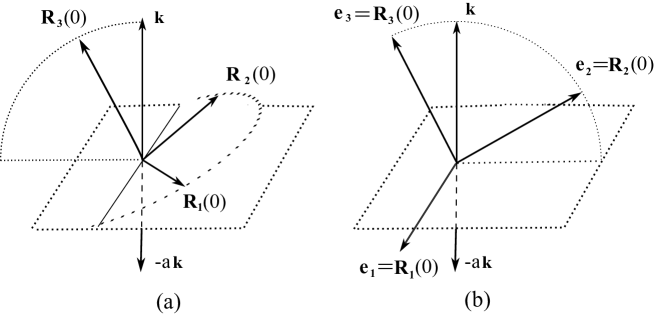
Figura 1: (a) - Initial position of a heavy body with orthogonal inertia axes ${\bf R}_{1}(0),{\bf R}_{2}(0),{\bf R}_{3}(0)$. (b) - For the symmetric body, due to the freedom in the choice of ${\bf R}_{1}(0)$ and ${\bf R}_{2}(0)$, the vector ${\bf k}$ can be taken in the form ${\bf k}=(0,k_{2},k_{3}).$

Let the initial position of the inertia axes ${\bf R}_{i}(0)$ of the body be as shown in Figure 1(a). Assuming that the Laboratory axes ${\bf e}_{i}$ have been chosen in the direction of the inertia axes, the matrices $g_{ij}$ and $I_{ij}$ in all equations acquire the diagonal form.

Doing the calculations similar to those of Sect. V of the work AAD23 , we can exclude the auxiliary variables $\lambda_{ij}$

$$\lambda_{ij}=\frac{2g_{i}g_{j}}{g_{i}+g_{j}}(\dot{\bf R}_{i},\dot{\bf R}_{i})-\frac{g_{i}({\bf R}_{i},{\bf F}_{j})+g_{j}({\bf R}_{j},{\bf F}_{i})}{g_{i}+g_{j}},\qquad\mbox{where}\qquad({\bf F}_{j})_{i}\equiv bk_{i}z_{j}(0),$$ (31)

and write closed equations of second-order for $R_{ij}$. The equivalent frst-order system is given then by $3+9$ Euler-Poisson equations

$$I\dot{\boldsymbol{\Omega}}=[I{\boldsymbol{\Omega}},{\boldsymbol{\Omega}}]+b[R^{T}{\bf k},{\bf z}(0)],\qquad\qquad$$ (32)

$$\dot{R}_{ij}=-\epsilon_{jkm}\Omega_{k}R_{im},\qquad\mbox{or}\qquad\dot{\bf G}_{i}=-[{\boldsymbol{\Omega}},{\bf G}_{i}].$$ (33)

From the line ${\bf k}=(k_{1},k_{2},k_{3})^{T}={\bf e}_{i}k_{i}={\bf e}_{i}R_{ij}(R^{T}{\bf k})_{j}={\bf R}_{j}(R^{T}{\bf k})_{j}$, we conclude that the functions $K_{j}(t)\equiv(R^{T}{\bf k})_{j}$ in Eq. (32) are components of the vector ${\bf k}$ in the body-fixed basis.

For the latter use we mention the identities

$$R^{T}{\bf k}=k_{i}{\bf G}_{i},\qquad[R^{T}{\bf k},{\bf z}(0)]_{i}=({\bf R}_{i}[{\bf k},{\bf z}(t)]).$$ (34)

They can be used to represent the torque of gravity in various equivalent forms.

Similarly to the free body, the Euler equations (32) are equivalent to the equations (26). Indeed, for the angular momentum in the body ${\bf M}=R^{T}{\bf m}$ the Eq. (26) implies

$$\dot{\bf M}=-[I^{-1}{\bf M},{\bf M}]+b[R^{T}{\bf k},{\bf z}(0)].$$ (35)

Since ${\bf M}=I{\boldsymbol{\Omega}}$, these are just the Euler equations.

Hamiltonian character of Euler-Poisson equations. The equations (32) and (33) represent a Hamiltonian system Dir_1950 ; GT ; deriglazov2010classical . This can be confirmed by constructing the Hamiltonian formulation of the Lagrangian theory (29) with help of intermediate formalism developed in the work AAD23_2 . This gives the Hamiltonian

$$H=\frac{1}{2}I_{ij}\Omega_{i}\Omega_{j}+bR_{ij}k_{i}z_{j}(0),$$ (36)

where $\Omega_{j}$ are Hamiltonian counterparts of the angular velocity in the body. The corresponding symplectic structure on phase space with the coordinates $R_{ij},\Omega_{k}$ is given by the Dirac brackets, that take into account the constraints $RR^{T}=1$ presented in the theory, and read as follows:

$$\{R_{ij},R_{kn}\}_{D}=0,\qquad\{\Omega_{i},\Omega_{j}\}_{D}=-\frac{I_{k}}{I_{i}I_{j}}\epsilon_{ijk}\Omega_{k},\qquad\{\Omega_{i},R_{jk}\}_{D}=-\frac{1}{I_{i}}\epsilon_{ikm}R_{jm}.$$ (37)

They coincide with the brackets suggested by Chetaev Chet_1941 as a symplectic structure of the theory (32) and (33), see AAD23 for the details. By construction, the Dirac brackets are degenerate, and $(RR^{T})_{ij}$ are their Casimir functions. In the Hamiltonian formalism, the Euler-Poisson equations acquire the form $\dot{q}^{A}=\{q^{A},H\}_{D}$, where $q^{A}$ is the set of phase-space variables $R_{ij},\Omega_{k}$.

Partial separation of variables in the Euler-Poisson equations. Assuming $k_{3}\neq 0$, consider the change of variables

$$({\boldsymbol{\Omega}},{\bf G}_{1},{\bf G}_{2},{\bf G}_{3})\rightarrow({\boldsymbol{\Omega}},{\bf G}_{1},{\bf G}_{2},{\bf K}),\qquad\mbox{where}\qquad{\bf K}=k_{i}{\bf G}_{i}=R^{T}{\bf k}.$$ (38)

Using the identities (34) we can separate $3+3$ equations of the system (32) and (33)

$$I\dot{\boldsymbol{\Omega}}=[I{\boldsymbol{\Omega}},{\boldsymbol{\Omega}}]+b[{\bf K},{\bf z}(0)],$$ (39)

$$\dot{\bf K}=-[{\boldsymbol{\Omega}},{\bf K}],\qquad\qquad$$ (40)

from the remaining $3+3$ equations

$$\dot{\bf G}_{1}=-[{\boldsymbol{\Omega}},{\bf G}_{1}],\qquad\dot{\bf G}_{2}=-[{\boldsymbol{\Omega}},{\bf G}_{2}].$$ (41)

Using (7), the integrals of motion (27), (28) can be rewritten as the integrals of motion of the system (39) and (40) as follows:

$$E=\frac{1}{2}I_{i}\Omega_{i}^{2}+b({\bf K},{\bf z}(0)),\qquad({\bf k},{\bf m})=({\bf K},I{\boldsymbol{\Omega}}),\qquad{\bf K}^{2}=1.$$ (42)

The equations (39) and (40) also form a Hamiltonian system with the Hamiltonian and brackets defined as follows:

$$H=\frac{1}{2}I_{ij}\Omega_{i}\Omega_{j}+b({\bf K},{\bf z}(0)),$$ (43)

$$\{K_{i},K_{j}\}_{D}=0,\qquad\{\Omega_{i},\Omega_{j}\}_{D}=-\frac{I_{k}}{I_{i}I_{j}}\epsilon_{ijk}\Omega_{k},\qquad\{\Omega_{i},K_{k}\}_{D}=-\frac{1}{I_{i}}\epsilon_{ikm}K_{m}.$$ (44)

Here ${\bf K}^{2}$ turns out to be the Casimir function of the brackets.

We emphasize once again that for asymmetric body $I_{1}\neq I_{2}\neq I_{3}$ there is no more a freedom to simplify the equations using a rotation of the Laboratory frame. In particular, the torque in Eq. (39) generally contains all three components of the vector ${\bf K}$. In component form, the equations (39) and (40) read as follows

$$\dot{\Omega}_{1}=\frac{I_{2}-I_{3}}{I_{1}}\Omega_{2}\Omega_{3}+\frac{b}{I_{1}}(K_{2}z_{3}-K_{3}z_{2}),\qquad\qquad$$ (45)

$$\dot{\Omega}_{2}=\frac{I_{3}-I_{1}}{I_{2}}\Omega_{1}\Omega_{3}+\frac{b}{I_{2}}(K_{3}z_{1}-K_{1}z_{3}),\qquad\qquad$$ (46)

$$\dot{\Omega}_{3}=\frac{I_{1}-I_{2}}{I_{3}}\Omega_{1}\Omega_{2}+\frac{b}{I_{3}}(K_{1}z_{2}-K_{2}z_{1}),\qquad\qquad$$ (47)

$$\dot{K}_{1}=\Omega_{3}K_{2}-\Omega_{2}K_{3},\quad\dot{K}_{2}=-\Omega_{3}K_{1}+\Omega_{1}K_{3},\quad\dot{K}_{3}=\Omega_{2}K_{1}-\Omega_{1}K_{2}.$$ (48)

Their formal solution can be written in terms of exponential of the Hamiltonian vector field, see AAD23_2 . For the center-of-mass vector ${\bf z}(0)$ in a general position, solution to these equations in quadratures is not known. There are two special cases, when the solution can be found in quadrarures: the Lagrange and Kovalevskaya tops.

IV Heavy symmetric body: Lagrange and Kovalevskaya tops.

Here we consider a symmetric body, that is $I_{1}=I_{2}\neq I_{3}$. Then the Euler equations (32) can be simplified: without loss of generality, we can assume that the vector ${\bf k}$ has the following form: ${\bf k}=(0,k_{2},k_{3})$. Indeed, the eigenvectors and eigenvalues of the inertia tensor $I$ obey the relations $I{\bf R}_{i}(0)=I_{i}{\bf R}_{i}(0)$. With $I_{1}=I_{2}$ we have $I{\bf R}_{1}(0)=I_{2}{\bf R}_{1}(0)$ and $I{\bf R}_{2}(0)=I_{2}{\bf R}_{2}(0)$, then any linear combination $\alpha{\bf R}_{1}(0)+\beta{\bf R}_{2}(0)$ also represents an eigenvector with eigenvalue $I_{2}$. This means that we are free to choose any two orthogonal axes on the plane ${\bf R}_{1}(0),{\bf R}_{2}(0)$ as the inertia axes. Hence, in the case $I_{1}=I_{2}$ we can rotate the Laboratory axes in the plane $(x^{1},x^{2})$ without breaking the diagonal form of the inertia tensor. Using this freedom, we can assume that $k_{1}=0$ for our problem, see Figure 1(b).

Lagrange top. Let us assume that the fixed point of the symmetric body was chosen such that center of mass lies on the third axis of inertia. Then at the initial instant of time we have ${\bf z}(0)=(0,0,1)^{T}$. This body is called the Lagrange top. Substituting ${\bf k}=(0,k_{2},k_{3})^{T}$ and ${\bf z}(0)=(0,0,1)^{T}$ into the Euler equations (32) we get

$$\dot{\Omega}_{1}=\phi\Omega_{2}+\frac{b}{I_{2}}(k_{2}R_{22}+k_{3}R_{32}),\qquad\dot{\Omega}_{2}=-\phi\Omega_{1}-\frac{b}{I_{2}}(k_{2}R_{21}+k_{3}R_{31}),\qquad\dot{\Omega}_{3}=0,$$ (49)

where $\phi=\frac{I_{2}-I_{3}}{I_{2}}\Omega_{3}=\mbox{const}$. Together with (33), they represent equations of motion of the Lagrange top. The last equation from (49) implies that besides the integrals of motion (27) and (28) there is one more: $\Omega_{3}=\mbox{const}$. This could be seen also from Eq. (35). Indeed, the third component of this equation reads as follows:

$$\dot{M}_{3}=\left(\frac{1}{I_{2}}-\frac{1}{I_{1}}\right)M_{1}M_{2}-b({\bf k},[{\bf R}_{3}(t),{\bf z}(t)]).$$ (50)

For the Lagrange top we have $I_{1}=I_{2}$ and ${\bf z}(t)={\bf R}_{3}(t)$, so $\dot{M}_{3}=I_{3}\dot{\Omega}_{3}=0$.

Variational problem for the Lagrange top in terms of Euler angles. Let us write the Lagrangian (29) as follows:

$$L=\frac{1}{2}I_{i}(\Omega_{i})^{2}-\frac{1}{2}\lambda_{ij}\left[R_{ki}R_{kj}-\delta_{ij}\right]-bR_{ij}(t)k_{i}z_{j}(0),$$ (51)

where $\Omega_{i}\equiv-\frac{1}{2}\epsilon_{ijk}(R^{T}\dot{R})_{jk}$. Let us substitute the expression for $R_{ij}$ in terms of Euler angles

$$R=\left(\begin{array}[]{ccc}\cos\psi\cos\varphi-\sin\psi\cos\theta\sin\varphi&-\sin\psi\cos\varphi-\cos\psi\cos\theta\sin\varphi&\sin\theta\sin\varphi\\ \cos\psi\sin\varphi+\sin\psi\cos\theta\cos\varphi&-\sin\psi\sin\varphi+\cos\psi\cos\theta\cos\varphi&-\sin\theta\cos\varphi\\ \sin\psi\sin\theta&\cos\psi\sin\theta&\cos\theta\end{array}\right)$$ (55)

into Eq. (51). According to classical mechanics, this gives an equivalent variational problem. Since the rotation matrix in terms of Euler angles authomatically obeys the constraint $R^{T}R={\bf 1}$, the second term of the action (51) vanishes, and we get

$$L=\frac{1}{2}I_{2}[\dot{\theta}^{2}+\dot{\varphi}^{2}\sin^{2}\theta]+\frac{1}{2}I_{3}[\dot{\psi}+\dot{\varphi}\cos\theta]^{2}-bR_{ij}(\theta,\varphi,\psi)k_{i}z_{j}(0).$$ (56)

As we saw above, the Lagrange top corresponds to the choice ${\bf z}(0)=(0,0,1)$ and $k=(0,k_{2},k_{3})$. With these ${\bf z}(0)$ and ${\bf k}$ the potential energy acquires the form $b(k_{2}R_{23}+k_{3}R_{33})$, and we get the variational problem for the Lagrange top in terms of Euler angles

$$L=\frac{1}{2}I_{2}[\dot{\theta}^{2}+\dot{\varphi}^{2}\sin^{2}\theta]+\frac{1}{2}I_{3}[\dot{\psi}+\dot{\varphi}\cos\theta]^{2}-b[k_{3}\cos\theta-k_{2}\sin\theta\cos\varphi].$$ (57)

This gives the following equations of motion

$$I_{3}[\dot{\psi}+\dot{\varphi}\cos\theta]=m_{\psi}=\mbox{const},$$ (58)

$$\frac{d}{dt}[I_{2}\dot{\varphi}\sin^{2}\theta+m_{\psi}\cos\theta]+bk_{2}\sin\theta\sin\varphi=0,$$ (59)

$$-I_{2}\ddot{\theta}+I_{2}\dot{\varphi}^{2}\sin\theta\cos\theta-m_{\psi}\sin\theta\dot{\varphi}+b[k_{3}\sin\theta+k_{2}\cos\theta\cos\varphi]=0.$$ (60)

Comment. In the textbooks, authors take a dfferent Lagrangian, the latter does not contain the term proportional to $k_{2}$ Arn_1 ; Landau_8

$$L_{A}=\frac{1}{2}I_{2}[\dot{\theta}^{2}+\dot{\varphi}^{2}\sin^{2}\theta]+\frac{1}{2}I_{3}[\dot{\psi}+\dot{\varphi}\cos\theta]^{2}-b\cos\theta.$$ (61)

This term is discarded on the base of the following reasoning: to simplify the analysis, choose the Laboratory axis ${\bf e}_{3}$ in the direction of the vector ${\bf k}$. However, this reasoning does not take into account the presence in the equations of moments of inertia, which have the tensor law of transformation under rotations. Indeed, going back to Eqs. (32) and (33), select ${\bf e}_{3}$ in Figure 1(b) in the direction of ${\bf k}$, and calculate the components of the inertia tensor. Since the axis of inertia ${\bf R}_{3}(0)$ does not coincide with ${\bf e}_{3}$, we obtain a symmetric matrix with non-zero off-diagonal elements (15) instead of (20). This symmetric matrix should now be used to construct the kinetic part of Lagrangian and hence it appears in the equations of motion. That is, the attempt to simplify the potential energy will lead, instead of (61), to a Lagrangian with a complicated expression for the kinetic energy.

Does a rotating body have motions that could be described using the equations following from (61)? The answer is yes: these are solutions with special initial conditions, for which the ${\bf R}_{3}(t)$ -axis coincides with ${\bf k}$ at some (finite) instant of time. These are the solutions of an awakened top and its limiting case of a sleeping top, see below. In the general case, to look for the solutions that do not pass through ${\bf k}$, one should use the equations following from (57).

Probably for the first time in the monographic literature the equations following from the Lagrangian (61) were discussed in details by MacMillan in Mac_1936 . In the absence of analytical solution in elementary functions, MacMillan performed analysis of integrals of motion and effective potential, reducing the problem to the study of a polinomial of degree 3. The results of this qualitative analysis are summarized in Figs. 60-62 of his book, and then reproduced in many other textbooks Gol_2000 ; Grei_2003 ; Arn_1 ; Landau_8 . In this respect we point out that a similar analysis of the improved Lagrangian (57) leads to the study of a polinomial of degree 6, see AAD23_5 .

Kovalevskaya top. Let us assume that the fixed point of the symmetric body was chosen such that center of mass lies in the plane of first and second inertia axes. Using rotation of the Laboratory axes at the initial instant of time, we can assume that ${\bf z}(0)=(1,0,0)^{T}$ (so, generally we have ${\bf k}=(k_{1},k_{2},k_{3})^{T}$). Using this ${\bf z}(0)$ in (47) and (48), we get the Euler-Poisson equations

$$\dot{\Omega}_{1}=\phi\Omega_{2}\Omega_{3},\qquad\dot{\Omega}_{2}=-\phi\Omega_{1}\Omega_{3}+\frac{b}{I_{2}}K_{3},\qquad\dot{\Omega}_{3}=-\frac{b}{I_{3}}K_{2},$$ (62)

$$\dot{K}_{1}=\Omega_{3}K_{2}-\Omega_{2}K_{3},\quad\dot{K}_{2}=-\Omega_{3}K_{1}+\Omega_{1}K_{3},\quad\dot{K}_{3}=\Omega_{2}K_{1}-\Omega_{1}K_{2},$$ (63)

where $\phi=\frac{I_{2}-I_{3}}{I_{2}}$. Remarcably, in addition to (27) and (28), this system also admits one more integral of motion. To see this, consider the following (complex) combinations of the equations of motion:

$$\frac{d}{dt}(\Omega_{1}+i\Omega_{2})=-\phi\Omega_{3}(\Omega_{1}+i\Omega_{2})+i\frac{b}{I_{2}}K_{3};$$ (64)

$$\frac{d}{dt}(K_{1}+iK_{2})=-i\Omega_{3}(K_{1}+iK_{2})+i(\Omega_{1}+i\Omega_{2})K_{3}.$$ (65)

Multipying the first on $(\Omega_{1}+i\Omega_{2})$, the second on $-i\frac{b}{I_{2}}$ and summing up, we exclude $K_{3}$

$$\frac{d}{dt}\left[\frac{1}{2}(\Omega_{1}+i\Omega_{2})^{2}-\frac{b}{I_{2}}(K_{1}+iK_{2})\right]=-i\left[\phi(\Omega_{1}+i\Omega_{2})^{2}-\frac{b}{I_{2}}(K_{1}+iK_{2})\right]\Omega_{3}.$$ (66)

Let us take $I_{3}=\frac{1}{2}I_{2}$, then $\phi$ in this equation turn into $\phi=\frac{1}{2}$. Denoting the resulting expression in square brackets of (66) by $Q$, this equation reads $\frac{d}{dt}\ln Q=-i\Omega_{3}$, and its conjugated is $\frac{d}{dt}\ln Q^{*}=i\Omega_{3}$. Summing up the two equations we get $\frac{d}{dt}(\ln QQ^{*})=0$, this gives the third integral of motion: $QQ^{*}=\mbox{const}$. This can be presented in the following form

$$\left[\Omega_{1}^{2}-\Omega_{1}^{2}-\frac{2b}{I_{2}}K_{1}\right]^{2}+\left[2\Omega_{1}\Omega_{2}-\frac{2b}{I_{2}}K_{2}\right]^{2}=c_{0}.$$ (67)

The symmetric body with $I_{1}=I_{2}=2I_{3}$ and with center of mass in the plane of the second and third inertia axes is called the Kovalevskaya top. Its solution in quadratures in modern form can be found in Per_2001 .

V Sleeping Lagrange top.

Consider the Lagrange top that at $t=0$ has its center-of-mass vector in the direction of gravity vector ${\bf k}$, and was launched with initial angular velocity $\Omega_{0}$=const around the axis ${\bf k}$. In accordance with this, we use ${\bf z}(0)={\bf k}=(0,0,1)^{T}$ and ${\boldsymbol{\Omega}}(0)=(0,0,\Omega_{0})$ in Eqs. (32), (33). The equations for $\Omega(t)$ and ${\bf R}_{3}(t)$ read as follows

$$\dot{\Omega}_{1}=\phi\Omega_{2}+\frac{b}{I_{2}}R_{32},\quad\dot{\Omega}_{2}=-\phi\Omega_{1}-\frac{b}{I_{2}}R_{31},\quad\dot{\Omega}_{3}=0;\qquad\qquad$$ (68)

$$\dot{R}_{31}=R_{32}\Omega_{3}-R_{33}\Omega_{2},\quad\dot{R}_{32}=R_{33}\Omega_{1}-R_{31}\Omega_{3},\quad\dot{R}_{33}=R_{31}\Omega_{2}-R_{32}\Omega_{1}.$$ (69)

They are satisfied by the functions ${\boldsymbol{\Omega}}(t)=(0,0,\Omega_{0})$, $R_{31}(t)=R_{32}(t)=0$ and $R_{33}(t)=1$. Then the remaining equations from (32), (33) are

$$\dot{R}_{11}=R_{12}\Omega_{0},\qquad\dot{R}_{12}=-R_{11}\Omega_{0},\qquad\dot{R}_{13}=0;$$ (70)

$$\dot{R}_{21}=R_{22}\Omega_{0},\qquad\dot{R}_{22}=-R_{21}\Omega_{0},\qquad\dot{R}_{23}=0.$$ (71)

Their general solution is

$$R_{11}=A\cos\Omega_{0}t+B\sin\Omega_{0}t,\quad R_{12}=-A\sin\Omega_{0}t+B\cos\Omega_{0}t,\quad R_{13}=F;$$ (72)

$$R_{21}=C\cos\Omega_{0}t+D\sin\Omega_{0}t,\quad R_{22}=-C\sin\Omega_{0}t+D\cos\Omega_{0}t,\quad R_{23}=G.$$ (73)

Taking into account the initial conditions $R_{ij}(0)=\delta_{ij}$, we get $A=D=1$, $B=C=F=G=0$, and the solution is the stationary rotation around the vector of gravity ${\bf k}$

$$R_{ij}(t)=\left(\begin{array}[]{ccc}\cos\Omega_{0}t&-\sin\Omega_{0}t&0\\ \sin\Omega_{0}t&\cos\Omega_{0}t&0\\ 0&0&1\end{array}\right).$$ (77)

VI Awakened Lagrange top.

Consider the Lagrange top that at $t=0$ has its center-of-mass vector in the direction of gravity vector ${\bf k}$, so ${\bf z}(0)={\bf k}=(0,0,1)^{T}$. Substituting these values into Eq. (51) we get the following variational problem in terms of Euler angles

$$L=\frac{1}{2}I_{2}[\dot{\theta}^{2}+\dot{\varphi}^{2}\sin^{2}\theta]+\frac{1}{2}I_{3}[\dot{\psi}+\dot{\varphi}\cos\theta]^{2}-b\cos\theta.$$ (78)

The initial conditions should be formulated now for the Euler angles. Let the top was lounched from vertical position with some linear velocity $\dot{\bf R}_{3}(0)$. This vector is parallel to the plane of the Laboratory vectors ${\bf e}_{1}$ and ${\bf e}_{2}$. Using the freedom to rotate the Laboratory system in the plane of these vectors without spoiling the diagonal form of the inertia tensor, we can assume that $\dot{\bf R}_{3}(0)$ is antiparallel to ${\bf e}_{2}$. With these agreements, consider the top with the initial position $\theta(0)=\varphi(0)=\psi(0)=0$, and with the initial nutation $\dot{\theta}(0)=\dot{\theta}_{0}$ and rotation $\dot{\psi}(0)=\dot{\psi}_{0}$, where $\dot{\theta}_{0}<<\dot{\psi}_{0}$. We do not fix the speed of precession $\dot{\varphi}(0)$ of azimyth plane because it is determined by $\dot{\psi}_{0}$, see Eq. (83) below. The Lagrangian (78) does not depend on $\psi$ and $\varphi$, so the equations of motion $\delta S/\delta\psi=0$ and $\delta S/\delta\varphi=0$ give the integrals of motion $m_{\psi}$ and $m_{\varphi}$

$$I_{3}[\dot{\psi}+\dot{\varphi}\cos\theta]=m_{\psi}=\mbox{const},\qquad\mbox{then}\quad m_{\psi}=I_{3}[\dot{\psi}_{0}+\dot{\varphi}_{0}],$$ (79)

$$I_{2}\dot{\varphi}\sin^{2}\theta+m_{\psi}\cos\theta=m_{\varphi}=\mbox{const}.\qquad\qquad$$ (80)

Substituting the initial condition $\theta(0)=0$ into the last equation, we conclude that the integrals of motion are not independent

$$m_{\varphi}=m_{\psi}.$$ (81)

Taking this into account, Eq. (80 ) reads

$$\dot{\varphi}=\frac{m_{\psi}}{I_{2}(1+\cos\theta)}.$$ (82)

This implies that $\dot{\varphi}$ is a non negative function, so the azimuth plane can not change its direction of rotation during the motion of the top. Besides, from the above expressions we get the initial speed $\dot{\varphi}_{0}$ and then the integral of motion $m_{\psi}$ through the initial rotation $\dot{\psi}_{0}$

$$\dot{\varphi}_{0}=\frac{I_{3}}{2I_{2}-I_{3}}\dot{\psi}_{0},\qquad m_{\psi}=\frac{2I_{2}I_{3}}{2I_{2}-I_{3}}\dot{\psi}_{0}.$$ (83)

Variation of the Lagrangian (78) with respect to $\theta$ gives the second-order equation

$$-I_{2}\ddot{\theta}+I_{2}\dot{\varphi}^{2}\sin\theta\cos\theta-I_{3}[\dot{\psi}+\dot{\varphi}\cos\theta]\dot{\varphi}\sin\theta+b\sin\theta=0.$$ (84)

Using Eqs. (79) and (83), we exclude the variables $\varphi$ and $\psi$, obtaining the closed equation for $\theta$

$$-I_{2}\ddot{\theta}-\frac{m_{\psi}^{2}}{I_{2}}\frac{\sin\theta}{(1+\cos\theta)^{2}}+b\sin\theta=0.$$ (85)

This equation follows from the effective Lagrangian

$$L_{eff}=\frac{I_{2}}{2}\dot{\theta}^{2}-\frac{m_{\psi}^{2}}{I_{2}(1+\cos\theta)}-b\cos\theta.$$ (86)

The energy of this effective one-dimensional problem is an integral of motion

$$\frac{I_{2}}{2}\dot{\theta}^{2}+\frac{m_{\psi}^{2}}{I_{2}(1+\cos\theta)}+b\cos\theta=E=\mbox{const},\qquad\mbox{then}\quad E=\frac{1}{2}[I_{2}\dot{\theta}_{0}^{2}+\frac{m_{\psi}^{2}}{I_{2}}]+b.$$ (87)

This allows us to write the first-order equation for $\theta$

$$\dot{\theta}=\sqrt{\frac{2}{I_{2}}}\sqrt{\frac{(E-b\cos\theta)(1+\cos\theta)-\gamma}{1+\cos\theta}},\qquad\mbox{where}\quad\gamma\equiv\frac{m_{\psi}^{2}}{I_{2}},$$ (88)

that can be immediately integrated

$$\int\frac{dx}{\sqrt{x[(E-b+bx)(2-x)-\gamma]}}=\sqrt{\frac{2}{I_{2}}}\int dt,\qquad\mbox{where}\quad x\equiv 1-\cos\theta.$$ (89)

So the problem was reduced to the elliptic integral appeared in the last expresssion.

In the absence of an analytic solution in terms of elementary functions, we can use the effective one-dimensional problem (86) for the qualitative analysis of the motion. Consider a top of mass $\mu=0,1$ kg, in the form of a cone of height $h=0,12$ m and radius $r=0,06$ m. As the fixed point we take the vertex of the cone. Then the distance to the center of mass and the inertia moments are Landau_8

$$L=\frac{3h}{4}=0,09m,\qquad I_{1}=I_{2}=\frac{3}{5}\mu(\frac{r^{2}}{4}+h^{2})=918\times 10^{-6},\qquad I_{3}=\frac{3}{10}\mu r^{2}=108\times 10^{-6}.$$ (90)

As the initial velocities of rotation and nutation we take $\dot{\psi}_{0}=2\pi n\leavevmode\nobreak\ rad/sec$ and $\dot{\theta}_{0}=0,2\leavevmode\nobreak\ rad/sec\sim 11^{\circ}/sec$, where $n$ is the number of revolutions per second. The potential energy of the effective problem (86) reads

$$U_{eff}(\theta)=\frac{\gamma}{1+\cos\theta}+b\cos\theta,\quad\mbox{where}\quad\gamma\equiv\frac{m_{\psi}^{2}}{I_{2}}=0,565694455\times 10^{-3},\quad b=a\mu L=0,0882.$$ (91)

Typical graphs of the function $U_{eff}(\theta)$ are drawn in the figure 2.

Figura 2: Effective potential energy of awakened Lagrange top with initial nutation rate $\dot{\theta}_{0}=11{}^{\circ}$/sec.

The potential energy of a slow top has a minimum at the point $\cos\theta=-1+\sqrt{\gamma/b}$, which shifts to the left with increasing the rotational speed $\dot{\psi}_{0}$, so that for velocities greater than $24$ revolutions per second the point of minimum becomes $\theta=0$. The graphs show that the awakened top first deviates from the vertical position, and then returns back.

The maximum deviation $\theta_{max}$ of the axis ${\bf R}_{3}(t)$ from the vertical can be found in analytical form from the equation (87), in which we should put $\dot{\theta}(t)=0$. Then

$$\cos\theta_{max}=\frac{\gamma+\sigma}{4b}-\sqrt{(1+\frac{\gamma+\sigma}{4b})^{2}-\frac{\gamma}{b}},\quad\mbox{where}\quad\delta=I_{2}\dot{\theta}_{0}^{2}=0,3672\times 10^{-4}.$$ (92)

Besides, with use of Eqs. (82) and (83) we can estimate the character of rotation of the azimyth plane by calculating the precession speed $\dot{\varphi}_{0}$ and $\dot{\varphi}(\theta_{max})$. The results of these calculations are presented in the table 1. The initial precession speed $\dot{\varphi}_{0}$ of the azimuth plane grows with $\dot{\psi}_{0}$, while the precession speed $\dot{\varphi}(\theta_{max})$ at the point of maximum deviation first decreases but then begins to increase, starting from 25 revolutions per second. The precession rate of a fast top changes slowly with time. Typical trajectory of the third axis ${\bf R}_{3}(t)$ is drawn in the Figure 3.

Tabela 1: Maximum deviation and precession rates of awakened Lagrange top with initial nutation rate $\dot{\theta}_{0}=11{}^{\circ}$/sec.

$\dot{\psi}_{0}=n$ rev./sec	$\theta_{max}{}^{\circ}$	$\dot{\varphi}_{0}$ rev./sec	$\dot{\varphi}(\theta_{max})$ rev./sec
1	175	0,0625	39
10	131	0,625	3,9
13	117	0,8	3,0
16	103	1	2,44
20	74	1,25	1, 95
23	46	1, 43	1,7
25	11	1,56	1,58
26	4	1,62	1,62

Figura 3: Trajectory of the axis ${\bf R}_{3}(t)$ (from vertical to the maximum deviation position) of awakened Lagrange top with initial nutation rate $\dot{\theta}_{0}=11{}^{\circ}$/sec.

VII Horizontal precession of the Lagrange top without nutation.

Consider the Lagrange top that at $t=0$ has its third axis ${\bf R}_{3}(0)$ orthogonal to the gravity vector ${\bf k}$, see Figure 4.

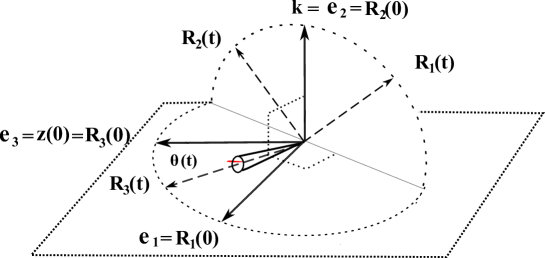
Figura 4: Horizontal precession of the Lagrange top without nutation.

Using the freedom of rotation of the Laboratory axes in the plane ${\bf e}_{1},{\bf e}_{2}$, we can assume that ${\bf k}={\bf e}_{2}=(0,1,0)^{T}$. Substituting these values together with ${\bf z}(0)=(0,0,1)^{T}$ into the Lagrangian (56), we get

$$L=\frac{1}{2}I_{2}[\dot{\theta}^{2}+\dot{\varphi}^{2}\sin^{2}\theta]+\frac{1}{2}I_{3}[\dot{\psi}+\dot{\varphi}\cos\theta]^{2}+b\sin\theta\cos\varphi.$$ (93)

This implies the equations

$$I_{3}[\dot{\psi}+\dot{\varphi}\cos\theta]=m_{\psi}=\mbox{const},$$ (94)

$$\frac{d}{dt}[I_{2}\dot{\varphi}\sin^{2}\theta+m_{\psi}\cos\theta]+b\sin\theta\sin\varphi=0,$$ (95)

$$-I_{2}\ddot{\theta}+I_{2}\dot{\varphi}^{2}\sin\theta\cos\theta-m_{\psi}\sin\theta\dot{\varphi}+b\cos\theta\cos\varphi=0.$$ (96)

We assume that our top has some initial rotation and precession rates $\dot{\psi}(0)=\dot{\psi}_{0}$ and $\dot{\theta}(0)=\dot{\theta}_{0}$. Then the initial position of the top is $\theta(0)=0,\varphi(0)=\frac{\pi}{2},\psi(0)=\frac{3\pi}{2}$. Let us look for a solution of the form $\theta(t),\varphi(t)=\frac{\pi}{2},\psi(t)$, then the equations of motion read

$$\dot{\psi}=\dot{\psi}_{0},\qquad\dot{\theta}=\frac{b}{I_{3}\dot{\psi}_{0}},\qquad\ddot{\theta}=0,$$ (97)

and we get the solution $\theta(t)=\frac{b}{I_{3}\dot{\psi}_{0}}t,\varphi(t)=\frac{\pi}{2},\psi(t)=\dot{\psi}_{0}t+\frac{3\pi}{2}$. Substituting these functions into Eq. (55) we obtain the rotation matrix which turns out to be the composition of two rotations: counterclockwise around ${\bf e}_{2}$ axis and clockwise around ${\bf e}_{3}$ axes

$$R(t)=\left(\begin{array}[]{ccc}\cos\dot{\psi}_{0}t\cos\dot{\theta}_{0}t&-\sin\dot{\psi}_{0}t\cos\dot{\theta}_{0}t&\sin\dot{\theta}_{0}t\\ \sin\dot{\psi}_{0}t&\cos\dot{\psi}_{0}t&0\\ -\cos\dot{\psi}_{0}t\sin\dot{\theta}_{0}t&\sin\dot{\psi}_{0}t\sin\dot{\theta}_{0}t&\cos\alpha t\end{array}\right)=\left(\begin{array}[]{ccc}\cos\dot{\theta}_{0}t&0&\sin\dot{\theta}_{0}t\\ 0&1&0\\ -\sin\dot{\theta}_{0}t&0&\cos\dot{\theta}_{0}t\end{array}\right)\times\left(\begin{array}[]{ccc}\cos\dot{\psi}_{0}t&-\sin\dot{\psi}_{0}t&0\\ \sin\dot{\psi}_{0}t&\cos\dot{\psi}_{0}t&0\\ 0&0&1\end{array}\right)$$ (107)

where

$$\dot{\theta}_{0}=\frac{b}{I_{3}\dot{\psi}_{0}}$$ (108)

Thus the Lagrange top lounched with the rotation rate $\dot{\psi}_{0}$ and precession rate $\dot{\theta}_{0}=\frac{b}{I_{3}\dot{\psi}_{0}}$ will precess without nutation in the horizontal plane. A slow spinning top must precess at high speed to stay on this plane. A fast spinning top precesses slowly. The relationship between frequencies of rotation and precession does not depend on the geometry of the top.

VIII Precession without nutation of inclined Lagrange top.

Without loss of generality, we can choose the initial position of inclined Lagrange top (and hence the Laboratory system) as shown in the Figure 5.

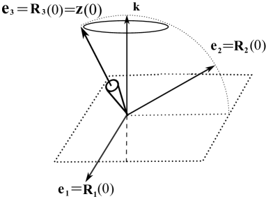
Figura 5: Precession without nutation of inclined Lagrange top.

According (49) and (33), the equations of motion are

$$\dot{\Omega}_{1}=\phi\Omega_{2}+\frac{b}{I_{2}}(k_{2}R_{22}+k_{3}R_{32}),\qquad\dot{\Omega}_{2}=-\phi\Omega_{1}-\frac{b}{I_{2}}(k_{2}R_{21}+k_{3}R_{31}),\qquad\Omega_{3}=\mbox{const};$$ (109)

$$\dot{R}_{ij}=-\epsilon_{jkm}\Omega_{k}R_{im},$$ (110)

where $\phi=\frac{I_{2}-I_{3}}{I_{2}}\Omega_{3}=\mbox{const}$. We look for the solution that represents precession without nutation, that is $({\bf R}_{3}(t),{\bf k})=\mbox{const}$ for any $t$. It can be expected that this motion be described by a rotation matrix consisting of the product of rotations around the axes ${\bf k}$ and ${\bf e}_{3}$: $R(t,\alpha,\gamma)=R_{{\bf k}}(t,\gamma)\times R_{{\bf e}_{3}}(t,\alpha)$. Therefore, we will look for a solution in the following form (see AAD23_4 for the details):

$$R_{ij}=\left(\begin{array}[]{ccc}\cos\gamma t\cos\alpha t-k_{3}\sin\gamma t\sin\alpha t&-\cos\gamma t\sin\alpha t-k_{3}\sin\gamma t\cos\alpha t&k_{2}\sin\gamma t\\ {}\hfil&{}\hfil&{}\hfil\\ k_{3}\sin\gamma t\cos\alpha t+(k_{2}^{2}+k_{3}^{2}\cos\gamma t)\sin\alpha t&-k_{3}\sin\gamma t\sin\alpha t+(k_{2}^{2}+k_{3}^{2}\cos\gamma t)\cos\alpha t&k_{2}k_{3}(1-\cos\gamma t)\\ {}\hfil&{}\hfil&{}\hfil\\ -k_{2}\sin\gamma t\cos\alpha t+k_{2}k_{3}(1-\cos\gamma t)\sin\alpha t&k_{2}\sin\gamma t\sin\alpha t+k_{2}k_{3}(1-\cos\gamma t)\cos\alpha t&k_{3}^{2}+k_{2}^{2}\cos\gamma t\end{array}\right)$$ (116)

with some frequences of rotation $\alpha$ and precession $\gamma$. For the positive values of the frequences, $R_{{\bf e}_{3}}(t,\alpha)$ ia a clockwise rotation while $R_{{\bf k}}(t,\gamma)$ is a counter-clockwise. Substituting this matrix into Eqs. (109) we get

$$\dot{\Omega}_{1}=\phi\Omega_{2}+\frac{bk_{2}}{I_{2}}\cos\alpha t,\qquad\dot{\Omega}_{2}=-\phi\Omega_{1}-\frac{bk_{2}}{I_{2}}\sin\alpha t.$$ (117)

The general solution to this system with two integration constants $c$ and $\phi_{0}$ is $\Omega_{1}=c\sin(\alpha t+\phi_{0})$, $\Omega_{2}=c\cos(\alpha t+\phi_{0})$, where

$$\alpha=\phi+\frac{bk_{2}}{I_{2}c}=\frac{I_{2}-I_{3}}{I_{2}}\Omega_{3}+\frac{bk_{2}}{I_{2}c}.$$ (118)

The initial conditions $R_{ij}(0)=\delta_{ij}$ imply $\phi_{0}=0$, so finally

$$\Omega_{1}=c\sin\alpha t,\qquad\Omega_{2}=c\cos\alpha t.$$ (119)

The functions (119) and (116) with $\alpha$ given in (118) satisfy the Euler equations (109) for arbitrary values of the constants $\Omega_{3}$, $c$ and $\gamma$. Let’s try to choose them so that our functions also satisfy the Poisson equations (110). At $t=0$ the equations (110) turn into $\Omega_{k}(0)=-\frac{1}{2}\epsilon_{kij}\dot{R}_{ij}(0)$. Substituting our functions (119) and (116) into these equalities we obtain the numbers $c$ and $\Omega_{3}$ through $\gamma$ as follows:

$$c=k_{2}\gamma,\qquad\Omega_{3}=\frac{b}{I_{3}\gamma}+\frac{I_{2}k_{3}}{I_{3}}\gamma.$$ (120)

Together with Eq. (118), these expressions give the following relationship between the two frequences of our problem:

$$\alpha=\frac{A}{\gamma}+Ck_{3}\gamma,\qquad\mbox{where}\quad A\equiv\frac{b}{I_{3}}=\frac{a\mu L}{I_{3}}>0,\quad C\equiv\frac{I_{2}-I_{3}}{I_{3}}.$$ (121)

It is verified by direct calculations that the functions (119) and (116) with these values of $c$, $\Omega_{3}$ and $\alpha$ satisfy the Poisson equations (110) for any value of the precession frequency $\gamma$. Hence the rotation matrix (116) with the rotation and precession frequences related according Eq. (121) describes the precession without nutation of inclined Lagrange top. Note that for the horizontal top, $k_{2}=1$ and $k_{3}=0$, the solution obtained turn into (107).

The function $\alpha(\gamma)$ depends on the top’s configuration $C$ and inclination $k_{3}$. To discuss this function, consider a conical top of height $h$, radius $r$ and the precession frequency $\gamma>0$. We get (see Eq. (90) $I_{2}-I_{3}=\frac{3\mu}{20}[4h^{2}-r^{2}]$. So $C>0$ when $h>r/2$ (high top), $C=0$ when $h=r/2$ (totally symmetric top, $I_{1}=I_{2}=I_{3}$ ), and $C<0$ when $h<r/2$ (low top).

Then the following cases arise.

A. The low top located above the horizon, that is

$$2h<r,\qquad\mbox{then}\quad C<0;\qquad k_{3}>0.$$ (122)

The graph of the function $\alpha(\gamma)$ is drawn in Figure 6(a), and implies the following behavior of the top.

Figura 6: The relationship between two frequences. (a) Low top located above the horizon, (b) High top located above the horizon.

A1. Slow precession without nutation, $\gamma<\gamma_{crit}=\sqrt{-b/(I_{2}-I_{3})k_{3}}$, implies a clockwise rotation of the top around ${\bf R}_{3}(t)$.

A2. When $\gamma=\gamma_{crit}$, the centripetal acceleration balances the force of gravity, and the top precesses without rotation around ${\bf R}_{3}(t)$.

A3. Rapid precession, $\gamma>\gamma_{crit}$, implies counter-clockwise rotation around ${\bf R}_{3}(t)$. In the limit $\gamma\rightarrow\infty$ the rotation frequency $|\alpha|$ grows linearly with $\gamma$.

B. The high top located below the horizon

$$2h>r,\qquad\mbox{then}\quad C>0;\qquad k_{3}<0,$$ (123)

has a similar bevavior.

C. The high top located above the horizon

$$2h>r,\qquad\mbox{then}\quad C>0;\qquad k_{3}>0.$$ (124)

The graph of the function $\alpha(\gamma)$ is drawn in Figure 6(b), and implies the following behavior of the top.

C1. The top rotating around ${\bf R}_{3}(t)$ with the frequency less than $\alpha(\gamma_{crit})=2\sqrt{(I_{2}-I_{3})bk_{3}}/I_{3}$ cannot precess without a nutation.

C2. There is only one rotation frequency $\alpha(\gamma_{crit})$ at which the top’s precession frequency is $\gamma_{crit}=\sqrt{b/(I_{2}-I_{3})k_{3}}$.

C3. For each $\alpha>\alpha(\gamma_{crit})$, there are two possible precession frequences for the movement without nutation

$$\gamma=\frac{\alpha\pm\sqrt{\alpha^{2}-4ACk_{3}}}{2Ck_{3}}.$$ (125)

D. The low top located below the horizon

$$2h<r,\qquad\mbox{then}\quad C<0;\qquad k_{3}<0,$$ (126)

has a similar bevavior.

E. The totally symmetrical conical top

$$2h=r,\qquad\mbox{then}\qquad I_{1}=I_{2}=I_{3},\qquad C=0,\qquad\alpha=\frac{b}{I_{3}\gamma},$$ (127)

has the behavior similar to the horizontal top. The relationship between two frequencies does not depend on the top’s inclination $k_{3}$.

IX Conclusion.

When formulating and solving the equations of motion of a rigid body with the inertia tensor chosen in the diagonal form, one should keep in mind the tensor law of transformation of the moments of inertia $I_{1},I_{2},I_{3}$ under rotations. We observed that for the Lagrange top this leads to the potential energy that depends on the Euler angles $\varphi$ and $\theta$. The potential energy (see the last term in (57)) is different from that assumed in textbooks (see the last term in (61)). As far as I know, this drawback has not yet been noticed and corrected in the literature. So we revised the problem of the motion of a Lagrange top and corrected this drawback. The problem of finding a general solution to the improved equations (58)-(60) can be reduced to the calculation of four elliptic integrals AAD23_5 . However, under some special initial conditions, one can either find analytical solutions in elementary functions or perform a qualitative analysis of the motion. We have found such solutions to the improved equations. The motions of an awakened and horizontally precessing Lagrange tops were analysed with use of unconstrained variables (Euler angles). The sleeping and inclined Lagrange tops were analysed in terms of original variables (rotation matrix $R_{ij}$ and angular velocity in the body $\Omega_{i}$). Perhaps somewhat unexpected is the motion of a high inclined top (the case C3): for a given rotation frequency greater than the critical one, it can precess without nutation at two different precession frequencies, see Eq. (125).