Solving Differential-Algebraic Equations in Power Systems Dynamics with Quantum Computing

Abstract

Power system dynamics are generally modeled by high dimensional nonlinear differential-algebraic equations due to a large number of generators, loads, and transmission lines. Thus, its computational complexity grows exponentially with the system size. In this paper, we aim to evaluate the alternative computing approach, particularly the use of quantum computing algorithms to solve the power system dynamics. Leveraging a symbolic programming framework, we convert the power system dynamics’ DAEs into an equivalent set of ordinary differential equations (ODEs). Their data can be encoded into quantum computers via amplitude encoding. The system’s nonlinearity is captured by Taylor polynomial expansion and the quantum state tensor whereas state variables can be updated by a quantum linear equation solver. Our results show that quantum computing can solve the dynamics of the power system with high accuracy whereas its complexity is polynomial in the logarithm of the system dimension.

I Introduction

Power system dynamics are generally modeled by a large number of differential-algebraic equations (DAEs) due to a large number of generators, loads, and transmission lines that form the network [1]. Specifically, the power system dynamics include a set of ordinary differential equations (ODEs) modeling the dynamics of synchronous generators along with algebraic nonlinear equations of power flow balances and Kirchhoff voltage laws for individual buses in the network. Solving such DAEs is a challenging task as they first need to be transformed into standard ODE forms, which is not a trivial task [2]. Then, the obtained ODEs can be solved by numerical discretization such as Euler, the Runge-Kutta, and the backward differentiation formula methods in classical computers [3]. However, the implementation on a classical computer scales exponentially with the size of the problem and the need of linearizing the nonlinear terms embedded in the complex power system dynamics, which often leads to high computational complexity [4, 3].

Quantum computer has a different way to perform computation and possesses algorithmically superior scaling for certain problems, e.g., the Harrow-Hassidim-Lloyd (HHL) algorithm linear equations [5]. The HHL algorithm is based on amplitude encoding, where a system with n variables can be represented as an n-level of quantum state $|\phi\rangle=\sum^{n}_{j}\phi_{j}|j\rangle$, in which $\phi_{j}$ is the amplitudes of computational basis states $|j\rangle$. Since the number of required qubits equals $\log_{2}(n)$, the algorithm provides an exponential memory advantage over the classical computing method [3]. Extending quantum linear equation solvers to tackle high-dimensional systems of linear ODEs are studied in [6, 7, 8]. Basically, they construct the quantum states proportional to the solution of the block-encoded $n$-dimensional system of linear equations, thus offering the prospect of rapidly characterizing the solutions of high-dimensional linear ODEs.

This paper aims to evaluate the potential of quantum computing for solving large-scale power system dynamics using quantum computing algorithms and recent advances in scientific computing frameworks. Unlike linear ODEs studied in [6, 7, 8], the power systems dynamics pose high-dimensional nonlinear DAEs. To this end, we leverage symbolic programming packages from Julia/SciML [9], particularly ModelingToolkit [10], to implement and transform power systems’ DAEs into an equivalent set of ODEs using the Pantelides based index reduction. Then, we employ Leyton’s quantum algorithm for nonlinear cases of ODEs [11]. Specifically, the obtained nonlinear ODEs are linearized by Taylor expansion as a set of polynomial functions of state variables. By storing multiple copies of quantum states, the nonlinearities embedded in polynomial functions are then captured by amplitudes of the tensor of quantum states. Then, state variables, which are updated in the classical computer according to the Euler method, are now equivalently updated using the HHL algorithm. The complexity, however, is polynomial to the logarithm of the system dimension.

The rest of the paper is organized as follows. The mathematical model of power systems dynamics are presented in Section II. The classical method for solving power system dynamics is presented in Section III. Section IV summarizes the quantum method to solve the power system dynamics. Section V illustrates the procedure to implement the power system dynamics into Julia, subsequently, transforming it to ODEs by ModelToolkit, and solving it by interfacing it with quantum simulator Yao/QuDiffEq. Section VI presents numerical studies on the SMIB and the three-machine nine-bus test systems. Section VII concludes the paper.

II Mathematical model

The dynamic circuit of a generic electric power network consisting of $m$ synchronous generators and $n$ buses, together with the power transmission network and the loads can be represented in Figure 1. Buses indexed $1,\ldots,m$ are generation buses and buses indexed $m+1,\ldots,n$ are load buses. Thus, the power grid can be considered a dynamics network represented by a set of Differential Algebraic Equations (DAEs) that consists of (i) a set of ordinary equations (ODEs) modeling the system dynamics of synchronous generators and (ii) a set of algebraic equations modeling generators’ stator voltage equations and power flow balances in the network [12].

II-A Dynamics of Generators

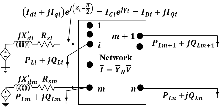
Figure 1: Interconnection of $m$ synchronous machine dynamic circuits and $n$ buses with network admittance matrix $\bar{Y}_{N}$ ($Y_{ik}\angle{\alpha_{ik}}$ represents the $\text{ik}^{\text{th}}$ element of $\bar{Y}_{N}$), $P_{Li}$ and $Q_{Li}$ as active and reactive power demands at buses $i$.

In Figure 1, the dynamic circuit of the generator in the two-axis $d$-$q$ coordinates [1] is considered as a constant voltage source behind impedance ($R_{si}+jX^{\prime}_{di}$) with an IEEE-Type I exciter. Its dynamics are represented by the following ODEs:

$$T^{\prime}_{qoi}\frac{\mathrm{d}E^{\prime}_{di}}{\mathrm{d}t} =-E^{\prime}_{di}+(X_{qi}-X^{\prime}_{qi})I_{qi}$$ (1a)

$$T^{\prime}_{doi}\frac{\mathrm{d}E^{\prime}_{qi}}{\mathrm{d}t} =-E^{\prime}_{qi}-(X_{di}-X^{\prime}_{di})I_{di}+E_{fdi}$$ (1b)

$$\frac{\mathrm{d}\delta_{i}}{\mathrm{d}t} =\omega_{i}-\omega_{s}$$ (1c)

$$\frac{2H_{i}}{\omega_{s}}\frac{\mathrm{d}\omega_{i}}{\mathrm{d}t} =T_{Mi}-E^{\prime}_{di}I_{di}-E^{\prime}_{qi}I_{qi}$$

$$-(X^{\prime}_{qi}-X^{\prime}_{di})I_{di}I_{qi}-D_{i}(\omega_{i}-\omega_{s})$$ (1d)

$$T_{Ei}\frac{\mathrm{d}E_{fdi}}{\mathrm{d}t} =-(K_{Ei}+S_{Ei}(E_{fdi}))E_{fdi}+V_{Ri}$$ (1e)

$$T_{Fi}\frac{\mathrm{d}R_{fi}}{\mathrm{d}t} =-R_{fi}+\frac{K_{Fi}}{T_{Fi}}E_{fdi}$$ (1f)

$$T_{Ai}\frac{\mathrm{d}V_{Ri}}{\mathrm{d}t} =-V_{Ri}+K_{Ai}R_{fi}$$

$$-\frac{K_{Ai}K_{Fi}}{T_{Fi}}E_{fdi}+K_{Ai}(V_{refi}-V_{i})$$ (1g)

$$\quad\quad\quad\quad\quad\quad\quad\quad\quad\quad\quad\quad\forall i=1,\ldots,m,$$

where $i$ is the generator index. The state variables of a generator $i$ include $d$-axis and $q$-axis internal voltages, $E^{\prime}_{di}$ and $E^{\prime}_{qi}$, the rotor angle, $\delta_{i}$, and the angular velocity, $\omega_{i}$. Their dynamics are captured in equations (1a)-(1d) respectively. The state variables of the exciter of the generator $i$ include the scaled field voltage $E_{fdi}$, the stabilizer rate feedback, $R_{fi}$, and the scaled input to the main, $V_{Ri}$, [13]. Their dynamics are captured in equations (1e)-(1g) respectively. The generator parameters used in (1) include $d$-axis and $q$-axis transient open-circuit time constants, $T^{\prime}_{do}$ and $T^{\prime}_{qo}$, the synchronous and transient reactances in $d$- and $q$-axis, $X_{d}$, $X^{\prime}_{d}$, $X_{q}$ and $X^{\prime}_{q}$, the synchronous angular speed, $\omega_{s}$, the inertia constant, $H$, the mechanical torque, $T_{M}$, and the damping coefficient, $D$. The parameters of the exciter and voltage stabilizer of the generator $i$ used in (1) include the exciter time constant, $T_{Ei}$, the exciter gain, $K_{Ei}$, exciter saturation, $S_{Ei}$, the rate feedback time constant, $T_{Fi}$, the rate feedback gain, $K_{Fi}$, the amplifier time constant, $T_{Ai}$, and the amplifier gain, $K_{Ai}$.

II-B Kirshoff voltage and network power flow equations

The stator currents $I_{di}$ $I_{qi}$ in $d$-$q$ coordinates of $m$ generators in buses $1,\ldots,m$, together with the magnitudes $V_{i}$ and phase angle $\theta_{i}$ of $n$ nodal voltages ($V_{i}\angle{\theta_{i}}$) in buses $1,\ldots,n$ are algebraic variables. For buses that have generators ($i=1,\ldots,m$), $I_{di}$, $I_{qi}$, and $V_{i}\angle{\theta_{i}}$ are coupled with the state variables of internal generators’ voltages, $E^{\prime}_{di}$ $E^{\prime}_{qi}$, by Kirchhoff voltage law as:

$$E^{\prime}_{di}-V_{i}\sin(\delta_{i}-\theta_{i})-R_{si}I_{di}+X^{\prime}_{qi}I_{qi}=0,$$ (2a)

$$E^{\prime}_{qi}-V_{i}\cos(\delta_{i}-\theta_{i})-R_{si}I_{qi}-X^{\prime}_{di}I_{di}=0,$$ (2b)

$$\forall i=1,\ldots,m,$$

where $R_{si}$ denotes the stator resistance and recall that $X^{\prime}_{di}$ denotes the transient reactance of generator $i$. Also, the active/reactive power balances for these generation buses are:

$$I_{di}V_{i}\sin(\delta_{i}-\theta_{i})+I_{qi}V_{i}\cos(\delta_{i}-\theta_{i})-P_{Li}$$

$$=\sum^{n}_{k=1}V_{i}V_{k}Y_{ik}\cos(\theta_{i}-\theta_{k}-\alpha_{ik})$$ (3a)

$$I_{di}V_{i}\cos(\delta_{i}-\theta_{i})-I_{qi}V_{i}\sin(\delta_{i}-\theta_{i})-Q_{Li}$$

$$=\sum^{n}_{k=1}V_{i}V_{k}Y_{ik}\sin(\theta_{i}-\theta_{k}-\alpha_{ik})$$ (3b)

$$\quad\quad\quad\quad i=1,\ldots,m,$$

where $$I_{di}V_{i}\sin(\delta_{i}-\theta_{i})+I_{qi}V_{i}\cos(\delta_{i}-\theta_{i}) I_{di}V_{i}\cos(\delta_{i}-\theta_{i})-I_{qi}V_{i}\sin(\delta_{i}-\theta_{i}) i n-m$$ and respectively are the active and reactive power generated by the generator at bus . Similarly, the active and reactive power balance equations for remaining load buses are:

$$-P_{Li}=\sum^{n}_{k=1}V_{i}V_{k}Y_{ik}\cos(\theta_{i}-\theta_{k}-\alpha_{ik})$$ (3c)

$$-Q_{Li}=\sum^{n}_{k=1}V_{i}V_{k}Y_{ik}\sin(\theta_{i}-\theta_{k}-\alpha_{ik})$$ (3d)

$$i=m+1,\ldots,n.$$

II-C DAE compact form

In short, the set of DAEs of power system dynamics can be written in the compact form [12, 13, 1].

$$\dfrac{\mathrm{d}x}{\mathrm{d}t}=f(t,x,y)$$ (4a)

$$0=g(t,x,y),$$ (4b)

$$x=[E^{\prime}_{di},E^{\prime}_{qi},\delta_{i},\omega_{i},E_{fi},R_{fi},V_{Ri}~{}~{}~{}(i=1,\ldots,n)]^{\top},$$

$$y=[I_{di},I_{qi},V_{i},\theta_{i}~{}~{}(i=1,\ldots,n)]^{\top},$$

where $f$ and $g$ are nonlinear vector-valued functions of state variables $x$, algebraic variables $y$, and time $t$. The dynamics of $m$ generators are composed in (4a) whereas the Kirchhoff voltage laws and power flow balance are encapsulated in (4b).

III Classical Methods for Power System Dynamics

Given a large number of algebra equations and variables in (4b), the power system dynamics in the form (4b) can be a DAE of index greater than two, which is very difficult to solve [14]. It needs to be transformed into an equivalent set of ODEs [2]:

$$\dfrac{\mathrm{d}z}{\mathrm{d}t}=\hat{f}(t,z)$$ (5)

where $z$ is a new set of state variables so it can be solved by existing ODE numerical methods [2] Such transformation, unfortunately, is a challenging task due to the complexity of nonlinear power flow equations embedded in (4b). If the Jacobian $\dfrac{\partial g}{\partial y}$ is nonsingular, i.e., the power flow and the Kirshoff voltage equations have a (unique) solution, which generally holds for normal operations of power systems. Based on the implicit function theorem, there exists a function $\hat{g}$ to equivalently convert (4b) into $y=\hat{g}(t,x)$. Thus, the formulation (4b) can be written in the standard form (5) by substituting $y$ by $\hat{g}(t,x)$, i.e., $\dfrac{\mathrm{d}x}{\mathrm{d}t}=f(t,x,\hat{g}(t,x))=\hat{f}(t,x)$. Unfortunately, we cannot explicitly model the nodal voltages (magnitudes and phases) as explicit functions of generators’ state variables, particularly, injected currents and internal voltages. Also, in many cases, the Jacobian $\dfrac{\partial g}{\partial y}$ can be singular depending on the operational points of the grid. To overcome these issues, this paper employs the Pantelides algorithm, a systematic method for reducing high-indexed DAEs to lower-indexed ones by selectively adding differentiated forms of the equations already in the system. This enables us to convert the power system dynamics (4b) into (5) where $z$ composes of original state variables $x$ and parts of variables $y$.

The formulation (5) is now in the standard form of ODEs and can be solved by numerical discretization methods [2] in classical computers such as the Forward Euler method:

$$\dfrac{z(t+\Delta)-z(t)}{\Delta}\approx\hat{f}(z(t)\iff z(t+\Delta)=z(t)+\Delta\hat{f}(z(t)),$$ (6)

which is indeed a linear equation.

IV Quantum Computing Method for Power System Dynamics

The linear equation (6) implies the potential application of advances in quantum computing for solving linear equations [5], for tackling the power system dynamics of a large-scale network. This includes the following steps [11].

IV-A Data encoding:

We encode the state vector $z$ in (6) of length $N$ into amplitudes of an n-qubit quantum state with $n=\log_{2}{N}+1$. Since the classical information $z$ now forms the amplitudes of a quantum state, the input $z$ needs to be normalized such that $\sum_{j=1}^{N}z_{j}=1$. We can encode the original state vector $z$ as the state of $n$-qubits as follows:

$$|{z}\rangle=\frac{1}{\sqrt{2}}|0\rangle+\frac{1}{\sqrt{2}}\sum_{j=1}^{n}\bar{z}_{j}|j\rangle,$$ (7)

where $|j\rangle$ is the computational basis for the Hilbert space. Thus, in principle, the forward Euler equation (6) can be equivalently implemented in a quantum computer as follows:

$$|z(t+\Delta)\rangle=|z(t)\rangle+\Delta|\hat{f}(\bar{z}(t)\rangle.$$ (8)

The remaining issue in (8) is how to construct the quantum state $|\hat{f}(z(t))\rangle$ with $\log_{2}(N)+1$ qubits from $|z(t)\rangle$. This can be achieved in quantum computers by combining Taylor expansion and mathematical tensor, which are described next.

IV-B Reformulate the state function using Taylor Expansion

The second-order Taylor polynomial approximation of the $j$-th element in $\hat{f}(z)$ is:

$$\hat{f}_{j}(z(t))\approx\hat{f}_{j}(z(t-\Delta))+\frac{\partial\hat{f}(z(t-\Delta))}{\partial z}(z(t)-z(t-\Delta))$$

$$+\frac{1}{2}(z(t)-z(t-\Delta))^{\top}Hf_{j}(z(t-\Delta))(z(t)-z(t-\Delta))$$

$$+O(\Delta^{2})$$ (9)

which can be rewritten in the form:

$$\hat{f}_{j}(z(t))=\underbrace{\hat{f}_{j}(z({t}{-}{\Delta}))}_{a^{j}_{0,0}}+\sum\limits_{k=1}^{N}a^{j}_{0,k}z_{k}(t)+\sum\limits_{v,k=1}^{N}a^{j}_{v,k}z_{v}(t)z_{k}(t)$$

where $a^{j}_{v,k},v=0,\ldots,N,k=0,\ldots N$ are coefficients resulted from Taylor expansion. Also, the first term $\hat{f}_{j}(z(t-\Delta))$ is known since it is computed at time step $t-\Delta$ and can be considered as $a^{j}_{0,0}$. Thus, by adding extra variable $z_{0}=1$, we have the following compact form of $\hat{f}_{j}$:

$$\hat{f}_{j}(z(t))=\sum\limits_{v,k=0}^{N}a^{j}_{v,k}z_{v}(t)z_{k}(t)$$ (10)

Computing $\hat{f}_{j}(z(t))$ requires encoding all monominals $z_{v}(t)z_{k}(t),\forall v,k$.

IV-C Nonlinear transformation of state function

A Quantum computer captures all values $z_{v}(t)z_{k}(t),\forall v,k$ in the probability amplitudes of the tensor product:

$$|z\rangle|z\rangle=\frac{1}{2}\sum^{N}_{v,k=0}z_{v}z_{k}|v\rangle|k\rangle,$$ (11)

where we need to make a copy of the quantum state $|z\rangle$. We now need an operator $A$ to assign corresponding coefficients, $a^{j}_{v,k}$, to individual monomial $z_{v}z_{k}$:

$$A=\sum\limits_{j,v,k=0}^{N}a^{j}_{v,k}|j0\rangle\langle vk|$$ (12)

Acting on $|z\rangle|z\rangle$ gives us the information of $\hat{f}(z)$:

$$A|z\rangle|z\rangle=\frac{1}{2}\sum\limits_{j,v,k=0}^{N}a^{j}_{v,k}z_{v}z_{k}|j\rangle|0\rangle=\frac{1}{\sqrt{2}}|\hat{f}(z)\rangle|0\rangle$$ (13)

The remaining question is how to simulate $A|z\rangle|z\rangle$ in a quantum computer, which is described next.

IV-D Simulation in a quantum computer

In order to simulate $A|z\rangle|z\rangle$, we can simply set up the following Hamiltonian using the well-known trick of von-Neumann measurement prescription [15]:

$$H=-iA\otimes|1\rangle_{P}\langle 0|+iA^{\dagger}\otimes|0\rangle_{P}\langle 1|$$ (14)

where $A^{\dagger}$ is the adjoin of $A$ and P is the adjoined qubit ”pointer”. If we simulate $H$ in the quantum computer with the initial state $|z\rangle|z\rangle|0\rangle_{P}$, the quantum system will evolve according to $H$ for a time $\epsilon$ and reach the steady state:

$$|\Psi\rangle =e^{i\epsilon H}|z\rangle|z\rangle|0\rangle=\sum\limits_{j=0}^{\infty}\frac{(i\epsilon H)^{j}}{j!}|z\rangle|z\rangle|0\rangle$$

$$=|z\rangle|z\rangle|0\rangle+\epsilon A|z\rangle|z\rangle|1\rangle-\ldots.$$ (15)

where the second term contains $A|z\rangle|z\rangle$. In other words, we simply need to measure the state quantum state $\Psi$ of the $n$-qubits and post-select on $|1\rangle$ to produce $|\hat{f}(z)\rangle$. As $|\hat{f}(z)\rangle$ can be simulated, the Forward Euler linear equation (6) can be solved by the HHL algorithm [5].

V Implementation with Scientific Machine Learning and Quantum Simulation Tools

We leverage recent advances in scientific machine learning to implement the aforementioned scientific computing algorithms as shown in Figure 2. This enables scalable/re-usable implementation of mathematical concepts such as Taylor expansion, ODEs/DAEs, and quantum algorithms, especially for different test cases of the power grid. The DAEs of power system dynamics to Julia, then use the ModelToolkit package in Julia, a symbolic equation-based model system, to convert DAEs to ODEs by index reduction method [10]. It transforms the DAEs to MTK symbolic representation, then uses dae_index_lowering to generate the index-1 form, particularly formulation (4b), which can be solved by ODE numerical methods in a classical computer. The ODEs obtained by MTK can also be solved by the solvers in the QuDiffEq package, which employs Yao as a quantum simulator. We employ the QuNLDE solver to linearize the ODE systems, and perform amplitude encoding, and Hamiltonian simulation.

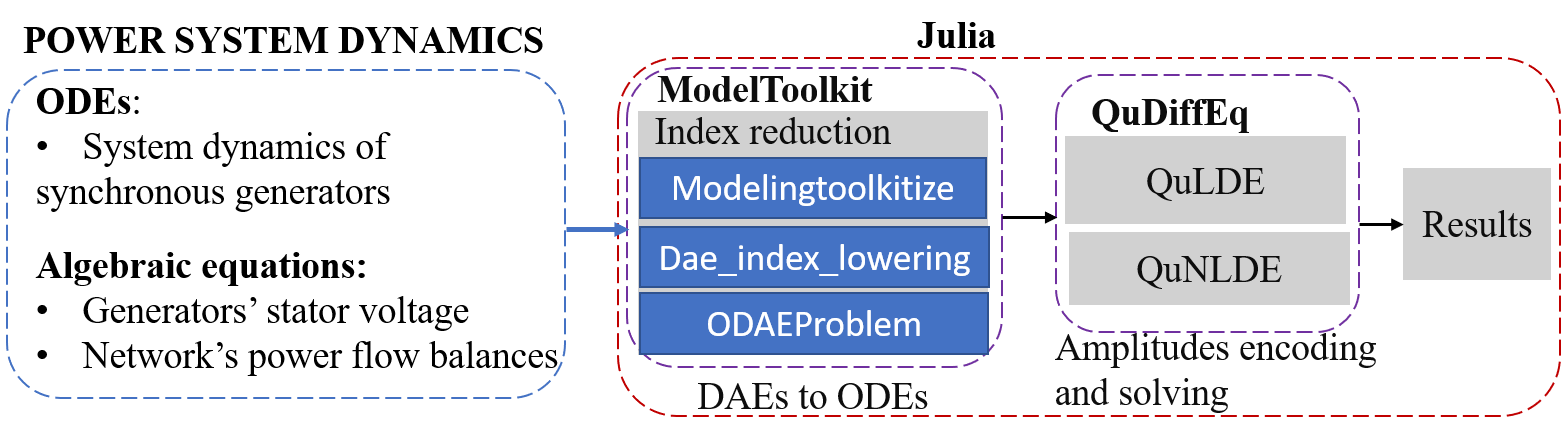
Figure 2: Implementation’s workflow.

VI Numerical Results

We solve the power system dynamics by quantum computing through two case studies including (i) a single-machine infinite bus system and (ii) Western System Coordinating Council (WSCC) three-machine nine-bus system. The time step for linearization is set as 0.01s. The difference between the quantum and classical methods is measured by the root means square error.

VI-A Single machine infinite bus system

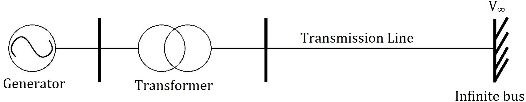
Figure 3: Single machine infinite bus system [13]

Figure 3 depicts a single-machine infinite bus (SIMB) system whose dynamics are in the simple ODE form [13]:

$$\frac{d\delta}{dt}=\omega-\omega_{s}$$ (16a)

$$\frac{2H}{\omega_{s}}\frac{d\omega}{dt}=P_{M}-\frac{E^{\prime}_{q}V}{X_{d\Sigma}}\sin(\delta)-\frac{D(\omega-\omega_{s})}{\omega_{s}}$$ (16b)

The parameters used in (16b) include the initial constant, $H$ = 15 kWs/kVA, synchronous angular speed, $\omega_{s}$ = 376.9911 rad/s, the mechanical power input of the synchronous machine, $P_{M}$ = 1 p.u., the voltage magnitude on the machine by $q$-axis, $E^{\prime}_{q}$ = 1.0566 p.u., the voltage of infinite bus, $V$ = 1 p.u., the total reactance by $d$-axis of the machine, $X_{d\Sigma}$ = 0.8805 p.u., and the damping constant, $D$ = 1.2. The SIMB system is equilibrium at $\delta_{0}$ = 0.9851 rad and $\omega_{0}=\omega_{s}$. We consider two cases when the initial generator’s angle departs from its equilibrium a) small disturbance, which $\Delta\delta=0.02$, the new $\delta_{0}=1.0051$ and b) large disturbance, which $\Delta\delta=0.4$, the new $\delta_{0}=1.3851$, while keeping $\omega_{0}=\omega_{s}$. The system oscillations derived from the initial values are shown in Figure 5. The solid line in Figure 5 represents the values of quantum computing, and the dashed line is the values of the classical method. It can be seen that for both situations quantum computing has the same value as the classical method with an error almost zero.

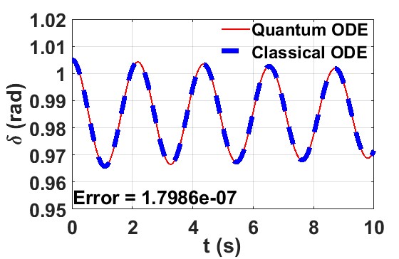
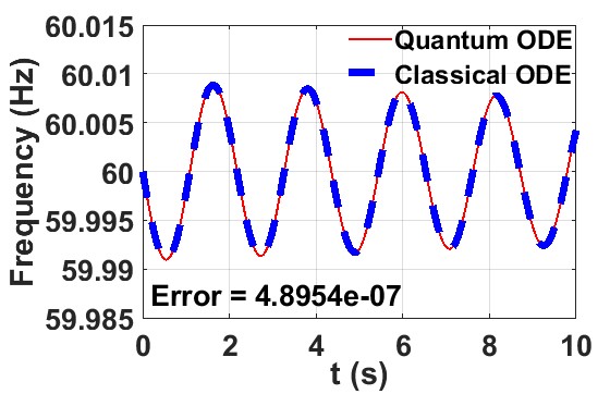
(a) Small disturbance

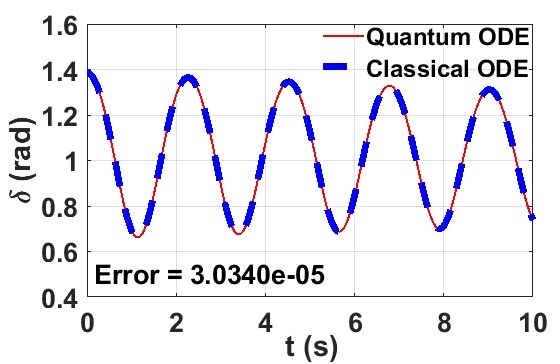
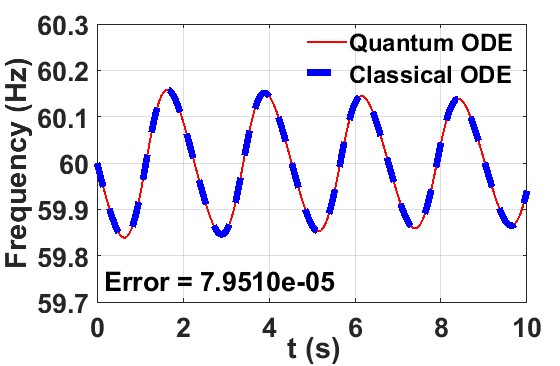
(b) Large disturbance

Figure 5: Results of SIMB system

VI-B WSCC three-machine nine-bus system

The WSCC system is shown in Figure 6 whose parameters and its equilibrium can be found in [1]. Its DAE system has 21 state variables and 24 algebraic variables, which are converted into ODEs with 39 state variables using Modelingtoolkit. At $t=0$, we consider an initial overvoltage occurs in the generator G1, i.e., its internal $q$-axis voltage, ${E^{\prime}}_{q,1}(0)$, is 0.45pu larger than the normal value, and its angle, $\delta_{1}(0)$, is 0.01pu increased from the equilibrium. Then, at $t=20s$, we consider the disturbances of load with two cases:

• Small disturbance: demands at B5, B6, and B7 increase by $0.2+j0.05$pu, $0.15$pu, and $0.2$pu respectively.

• Large disturbance: demands at B5, B6, and B7 increase by $0.5+j0.25$pu, ${0.3}{+}{j}{0.05}$pu, and ${0.4}{+}{j}$0.05pu respectively.

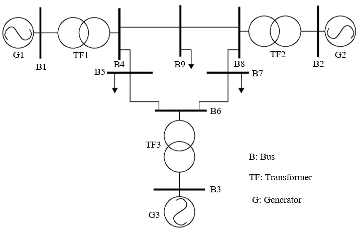
Figure 6: WSCC three-machine nine-bus system [13, 1]

Figures 8-10-12 show the changes of variables (frequency, $f_{i}=\dfrac{\omega_{i}}{2\pi}$, the scaled field voltage, $E_{fd}$, and the stabilizer rate feedback $R_{f}$ of the exciter system, and active power output, $P_{e}$ corresponding to generators G1, G2, and G3 ($i=1,2,3$) respectively). It is observed that $t=0$s to $t=20$s, all generators’ variables oscillate for a few seconds from the initial values before reaching and returning to the equilibrium values. The variation of $E_{fd}$ and $R_{f}$ illustrates the operations of generators’ exciters to stabilize over-voltage issues occurring at $t=0$. When the load changes at $t=20s$, the active powers generated by generators all increase to compensate for the increased loads whereas their frequencies reduce. A larger change in loads leads to a higher change of generators’ variables when we compare the results in Figures 8a-10a-12a and the results in in Figures 8b-10b-12b.

These results are used to validate the potential of quantum computing for modeling system dynamics. The solid line in Figures 8-10-12 represents the values obtained by quantum computing whereas the dashed line is the values obtained by the classical Forward Euler method. In both periods ( $0\leq t<20$ and $t\geq 20$), quantum solvers simulate well the system dynamics induced by the initial setting values of system variables as well as the changes of loads. The differences between results obtained by quantum-based and classical methods are measured by the RMSE metric. Compared to the SMIB case, the errors are larger due to the higher complexity of the WSCC test cases along with the DAEs modeling the system dynamics instead of the purely ODEs used in the SMIB. However, these errors are very small and acceptable.

VII Conclusion

This paper presents the method of quantum computing to solve the power system dynamics, which is typically represented as a set of DAEs and can be converted into a set of ODEs using the index reduction method. Their data can be encoded into quantum computers by using amplitude encoding, which requires a number of qubits as a logarithm of the number of state variables. To this end, the nonlinear ODEs need to be linearized as a set of polynomial functions of state variables to be simulated in quantum computers by amplitudes of tensors and tailored Hamiltonian tricks. The linear update in traditional ODE solvers can be replaced by quantum-based linear solvers, such as the HHL algorithm with proven quantum advantages. Our numerical results demonstrate the potential of quantum computing in modeling power system dynamics with high accuracy. Additionally, we also illustrate the use of scientific machine learning tools, particularly symbolic programming, to facilitate the use of scientific computing concepts, e.g., Taylor expansion, DAEs/ODEs transform, and quantum solver, in the field of power engineering.

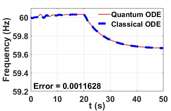
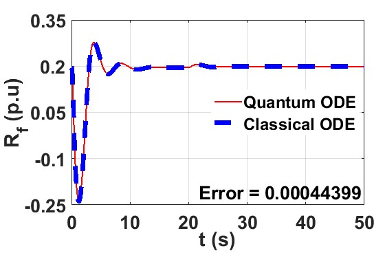
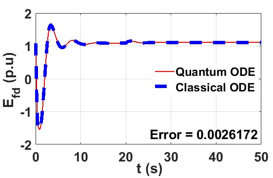
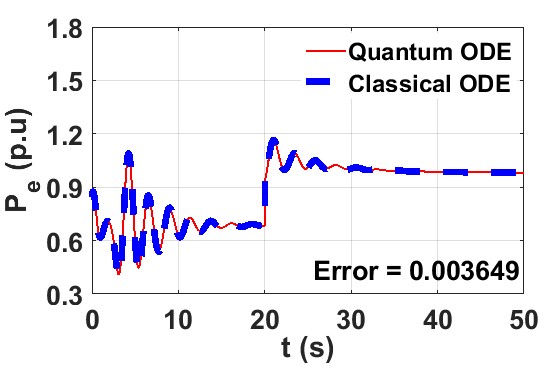
(a) Small change of loads

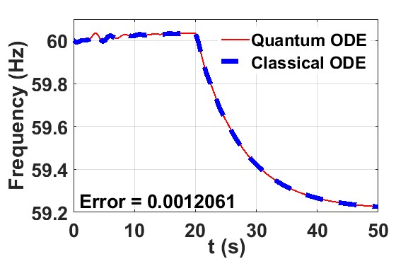
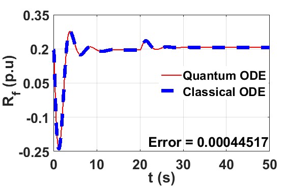
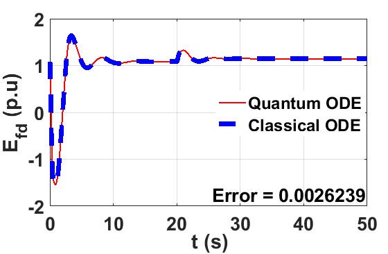
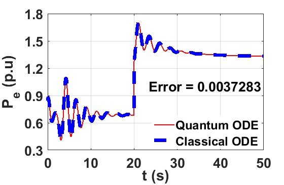
(b) Large change of loads

Figure 8: Generator 1

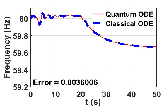
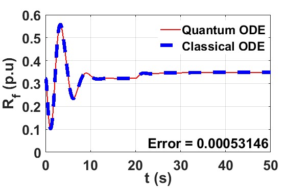
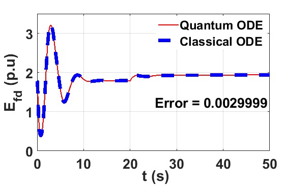
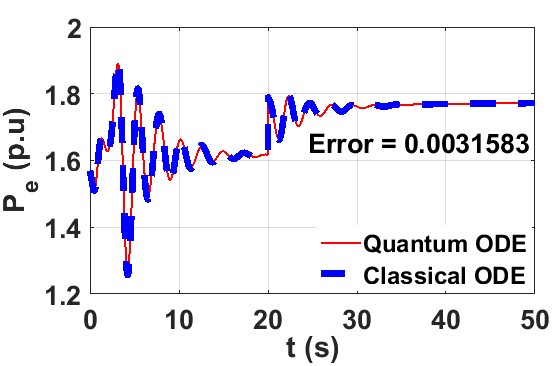
(a) Small change of loads

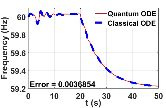
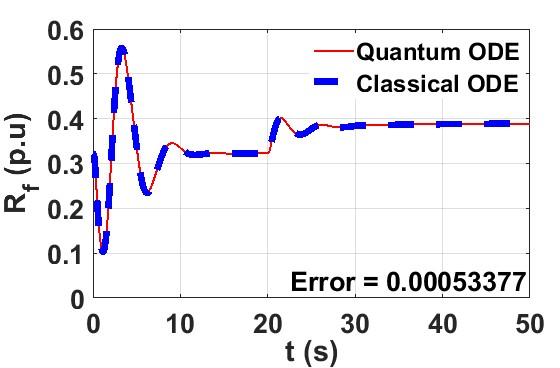
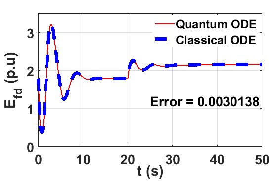
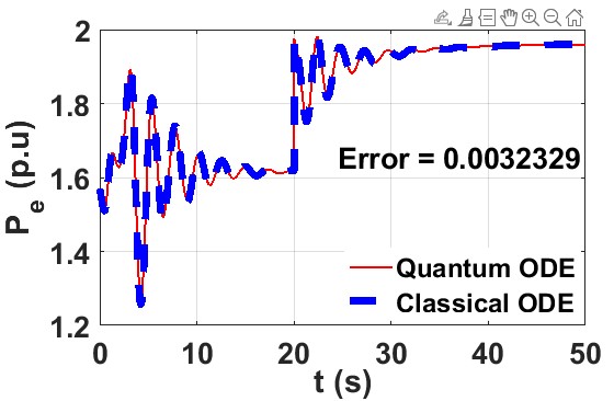
(b) Large change of loads

Figure 10: Generator 2

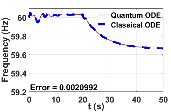
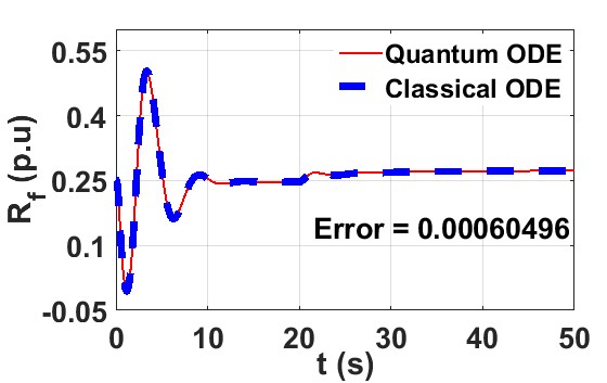
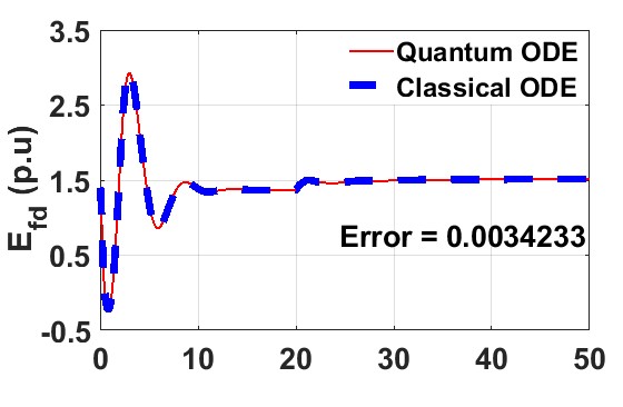
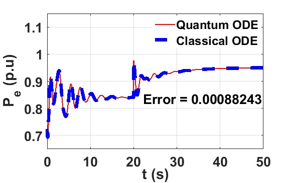
(a) Small change of loads

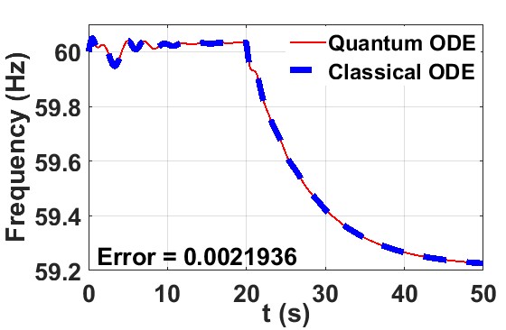
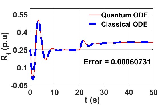
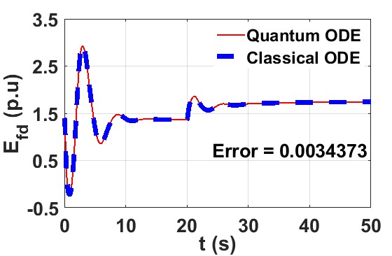
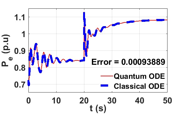
(b) Large change of loads

Figure 12: Generator 3

References

- [1] P. W. Sauer, M. A. Pai, and J. H. Chow, Power system dynamics and stability: with synchrophasor measurement and power system toolbox. John Wiley & Sons, 2017.
- [2] U. M. Ascher and L. R. Petzold, Computer methods for ordinary differential equations and differential-algebraic equations. Siam, 1998, vol. 61.
- [3] O. Kyriienko, A. E. Paine, and V. E. Elfving, “Solving nonlinear differential equations with differentiable quantum circuits,” Physical Review A, vol. 103, no. 5, p. 052416, 2021.
- [4] J. Stiasny, S. Chatzivasileiadis, and B. Zhang, “Solving differential-algebraic equations in power systems dynamics with neural networks and spatial decomposition,” arXiv preprint arXiv:2303.10256, 2023.
- [5] A. W. Harrow, A. Hassidim, and S. Lloyd, “Quantum algorithm for linear systems of equations,” Physical review letters, vol. 103, no. 15, p. 150502, 2009.
- [6] D. W. Berry, “High-order quantum algorithm for solving linear differential equations,” Journal of Physics A: Mathematical and Theoretical, vol. 47, no. 10, p. 105301, 2014.
- [7] A. M. Childs, R. Kothari, and R. D. Somma, “Quantum algorithm for systems of linear equations with exponentially improved dependence on precision,” SIAM Journal on Computing, vol. 46, no. 6, pp. 1920–1950, 2017.
- [8] T. Xin, S. Wei, J. Cui, J. Xiao, I. Arrazola, L. Lamata, X. Kong, D. Lu, E. Solano, and G. Long, “Quantum algorithm for solving linear differential equations: Theory and experiment,” Physical Review A, vol. 101, no. 3, p. 032307, 2020.
- [9] C. Rackauckas and Q. Nie, “Differentialequations.jl–a performant and feature-rich ecosystem for solving differential equations in julia,” Journal of Open Research Software, vol. 5, no. 1, p. 15, 2017.
- [10] Y. Ma, S. Gowda, R. Anantharaman, C. Laughman, V. Shah, and C. Rackauckas, “Modelingtoolkit: A composable graph transformation system for equation-based modeling,” 2021.
- [11] S. K. Leyton and T. J. Osborne, “A quantum algorithm to solve nonlinear differential equations,” arXiv preprint arXiv:0812.4423, 2008.
- [12] D. J. Hill and G. Chen, “Power systems as dynamic networks,” in 2006 IEEE International Symposium on Circuits and Systems (ISCAS). IEEE, 2006, pp. 4–pp.
- [13] S. Wang, W. Gao, and A. S. Meliopoulos, “An alternative method for power system dynamic state estimation based on unscented transform,” IEEE transactions on power systems, vol. 27, no. 2, pp. 942–950, 2011.
- [14] L. Petzold, “Differential/algebraic equations are not ode’s,” SIAM Journal on Scientific and Statistical Computing, vol. 3, no. 3, pp. 367–384, 1982.
- [15] A. Peres, Quantum theory: concepts and methods. Springer, 1997.