ASTRA: a Transition-Density-Matrix Approach to Molecular Ionization

Abstract

We describe astra (AttoSecond TRAnsitions), a new close-coupling approach to molecular ionization that uses many-body transition density matrices between ionic states with arbitrary spin and symmetry, in combination with hybrid integrals between Gaussian and numerical orbitals, to efficiently evaluate photoionization observables. Within the transition-density-matrix approach, the evaluation of inter-channel coupling is exact and does not depend on the size of the configuration-interaction space of the ions. Thanks to these two crucial features, astra opens the way to studying highly correlated and comparatively large targets at a manageable computational cost. Here, astra is used to predict the parameters of bound and autoionizing states of the boron atom and of the N₂ molecule, as well as the total photoionization cross section of boron, N₂, and formaldehyde, H₂CO. Our results are in excellent agreement with theoretical and experimental values from the literature.

I Introduction

Excitation of correlated electronic motion is at the core of light-induced chemical transformations in matter Kraus and Wörner (2018). The advent of attosecond spectroscopies Hentschel et al. (2001); Paul et al. (2001); Krausz and Ivanov (2009) has made it possible to study electron dynamics on its natural sub-femtosecond timescale Nisoli et al. (2017); Palacios and Martín (2020); Borrego-Varillas et al. (2022); Leone and Neumark (2023). Continuous advances in the XUV and soft-x-ray ultrafast technologies, pursued at large free-electron-laser facilities Feldhaus et al. (2013); Hartmann et al. (2018) as well as in several attosecond laboratories around the world Popmintchev et al. (2010); Sansone et al. (2011); Chini et al. (2014); Calegari et al. (2016); Kühn et al. (2017); Midorikawa (2022), have continued extending the range of attosecond-pulse parameters to still shorter durations, larger intensities, energies, and repetition rates Saito et al. (2019); Duris et al. (2020); Callegari et al. (2021); Mirian et al. (2021). At the same time, the focus of attosecond experiments has moved from atomic systems and small molecules to larger systems with chemical and biological relevance Calegari et al. (2014); Ueda et al. (2019); Månsson et al. (2021).

Attosecond pump-probe observables, such as coincidence photoelectron distributions and transient absorption spectra, are complex functions of the laser parameters that reflect the correlated and entangled dynamics of the probed system only indirectly. Due this complexity, ab initio methods beyond the single-particle approximation are essential to reconstruct and ultimately control the many-body motion excited by short light pulses Armstrong et al. (2021).

Here we present astra (AttoSecond TRAnsitions), a wave-function close-coupling approach based on a new transition-density-matrix close-coupling (TDMCC) formalism, suited to describe ab initio the ionization processes that are made accessible by the use of new sources of coherent ultrashort light. astra is designed to describe both atoms and larger molecules, for both low- and high-energy photoelectrons. It takes exchange and correlation into account to the full extent allowed by state-of-the-art large-scale configuration-interaction quantum-chemistry methods Olsen (2000a). astra admits a natural extension to double-ionization processes, which are needed to observe the motion of correlated electron pairs in real time, as well as to multiple disjoint molecular fragments that share electrons. Thanks to these properties, astra promises to appreciably expand the capabilities made available by existing molecular ionization codes.

This paper is organized as follows. Sec. II gives a short overview of the theoretical methods currently available or under active development to describe the ionization of polyelectronic molecular systems, and where astra fits in this context. Sec. III defines the close-coupling (CC) states Burke and Schey (1962), the expressions for arbitrary operators within the TDMCC formalism, and relevant observables. Sec. IV illustrates how TDMCC is numerically implemented in astra. Sec. V presents astra results for the boron atom, the nitrogen molecule, and formaldehyde. Sec. VI offers conclusions and perspectives. Appendix A summarizes second-quantization formalism. Appendix B introduces Transition Density Matrices and their spin-adapted reduced counterparts. Appendix C details the derivation of the matrix elements between spin-adapted close-coupling states. Finally, App. D summarizes the CI-singles approximation.

II Context 

A broad group of many-body methods for atomic and molecular ionization assumes a single-reference for both the initial bound state and the final state in the continuum. These include: the xatom Rudek et al. (2012) and xmolecule codes Hao et al. (2019), suited for estimating fragment yields following multiple sequential ionization steps by intense x-ray Free-Electron Lasers (XFEL) pulses Rudenko et al. (2017); the e-Polyscat code Natalense and Lucchese (1999); Gong et al. (2022), which has been applied to single-photon and multiphoton single ionization in the static-exchange approximation; tiresia B-spline density-function method, based on single center Venuti et al. (1998); Stener and Decleva (1998) and polycentric expansion Toffoli et al. (2002); Decleva et al. (2022), which was applied to strong-field ionization Petretti et al. (2010), core photoionization Canton et al. (2011); Plésiat et al. (2012); Argenti et al. (2012), pump-probe ionization of molecules with biological relevance Calegari et al. (2014); Lara-Astiaso et al. (2018), and high-harmonic generation Neufeld et al. (2019); octopus, a general-purpose time-dependent density-function theory (TDDFT) grid method applicable also to attosecond photoelectron spectroscopy De Giovannini et al. (2012) and transient-absorption spectroscopy De Giovannini et al. (2013). While single-reference methods reproduce the essential features of strong-field ionization processes Awasthi et al. (2008) of core photoelectron spectroscopy Kukk et al. (2013) and of processes that lead to the complete fragmentation of a target Ayuso et al. (2014), wave-function-based multi-reference approaches are needed for those cases in which multiply excited states and the entanglement between photo-fragments play a fundamental role.

Time-dependent (TD) multi-configuration (MC) self-consistent-field (SCF) approaches offer a compact description for the wave function. These include multi-configuration TD Hartree Lode et al. (2020) and Hartree-Fock Haxton et al. (2011); Sawada et al. (2016); Liao et al. (2017), TD restricted-active-space (RAS) SCF Miyagi and Madsen (2013); Omiste and Madsen (2021), TD generalized-active-space (GAS) SCF Bauch et al. (2014); Chattopadhyay et al. (2015), TD complete-active-space (CAS) SCF Sato and Ishikawa (2013), TDMCSCF Li et al. (2021), and TD coupled-cluster methods Sato et al. (2018). These methods are effective for optical observables, whereas photoelectron observables are more difficult to converge since parent ions evolve even in the asymptotic limit, in absence of fields.

The remaining methods rely on the close-coupling approach (CC), which guarantees the correct asymptotic behavior of the wave function, and they give rise to a stable linear evolution. These methods differ in the level of accuracy with which the ions are represented, in the approximations made to evaluate the matrix elements between CC states, and in the limits imposed to the size and energy of the system.

In its simplest configuration-interaction singles (CIS) formulation Toffoli and Decleva (2016); Hoerner et al. (2020); Carlström et al. (2022), the CC space is described by single excitations from a reference single-determinantal function.

More general close-coupling approaches include correlation in the $N-1$-electron parent ions, as well as localized $N$-electron configurations to reproduce the short-range correlation of the neutral system in either bound or continuum states. Furthermore, different methods adopt different ways of reconciling the convenience of Gaussian-type orbitals (GTO) to describe bound states with the need of employing numerical bases to represent diffuse Rydberg and continuum orbitals, such as monocentric Bachau et al. (2001) and polycentric Toffoli et al. (2002) B-splines, or monocentric Yip et al. (2008) and polycentric FEDVR functions Greenman et al. (2017).

The R-matrix method for molecular ionization Burke et al. (1977), originally implemented for electron scattering and stationary regimes (ukrmol) Gorfinkiel and Tennyson (2005), has recently been extended to time-dependent photoionization processes (ukrmol+) Harvey et al. (2014); Mašín et al. (2020); Brown et al. (2020). ukrmol+ employs hybrid Gaussian B-spline bases, and it can deal with arbitrary hybrid integrals. The K-matrix RPA approach has been applied to one- and two-photon transitions in stationary regime Cacelli (1991); Cacelli et al. (2001).

The Complex-Kohn approach, based on the mesa program, (ck-mesa) has the unique feature of representing the effect of short-range correlation by means of an optical potential from a large CI space, which leads to accurate electron-scattering and one-photon photoionization amplitudes Schneider and Rescigno (1988); McCurdy and Rescigno (1989); Schneider et al. (1990); Rescigno et al. (1993); Williams et al. (2012). Recently, ck-mesa has been extended to two-photon transitions and applied to resonant pump-probe process Douguet et al. (2018). The time-dependent Recursive indeXing code (t-Recx) is a general software for the ab initio solution of large-scale time-dependent problems in atomic and molecular physics, including close coupling in a hybrid basis Majety and Scrinzi (2015); Scrinzi (2022).

The xchem code circumvents the need of computing some exchange terms in the close-coupling Hamiltonian and some hybrid bielectronic integrals by confining the molecular ion in a spherical region in which all electronic states are expanded in terms of GTOs Marante et al. (2017a, b); Klinker et al. (2018a, b); Marggi Poullain et al. (2019); Borràs et al. (2021, 2023). The polycentric B-spline basis developed for the tiresia code has recently been co-opted for the development of a novel molecular ionization code based on the algebraic diagrammatic construction (ADC) to represent correlated many-body states Ruberti et al. (2018); Ruberti (2019). The Multi-Channel Schwinger Configuration Interaction Method (mcsci), an established method for molecular photoionization, based on the graphical unitary group approach Bandarage and Lucchese (1993); Stratmann and Lucchese (1995), has also been applied to the description of time-resolved photoelectron spectroscopy in linear molecules Lucchese et al. (2007).

astra belongs to the latter group of most general CC methods. It differs from the methods above because it relies on a TDMCC formalism. In astra, the intricacies of the many-body interactions within the parent ions and between the ions and the photoelectron(s) are confined to the n-point correlation functions of highly correlated ionic states, which are efficiently computed by a large-scale-CI bound-state code. The computational cost for CC observables is independent of the size of the CI space for the ion. Exchange terms are treated exactly, so that the size of the target and the photoelectron energy are not constrained. astra predictions are in excellent agreement with theoretical and experimental benchmarks for atoms and small molecules.

III TDMCC formalism

III.1 The Close-Coupling Ansatz

In single photoionization processes, an initially bound molecular system $\mathrm{M}$ breaks into a photoelectron and a bound state $A$ of the $\mathrm{M}^{+}$ molecular parent ion. In the case of the absorption of a single photon $\gamma$ from the ground state, for example, the process reads

$$\mathrm{M}_{g}+\gamma\longrightarrow\mathrm{M}^{+}_{A}+e^{-}.$$ (1)

Once the two charged fragments are far apart, the parent ion can be found in only a finite number of states, i.e., all those permitted by conservation of energy, $E_{\mathrm{A}}-E_{g}<\hbar\omega_{\gamma}$, where $\omega_{\gamma}$ is the photon frequency. When the parent ion and electron are well separated, the configuration space may be represented by a linear combination of parent ions times arbitrary one-particle states for the photoelectron,

$$\Psi\simeq\hat{\mathcal{A}}_{N}{\sum}_{A,P}c_{A,P}[\Phi_{A}(\mathbf{x}_{1}\cdots\mathbf{x}_{N-1})\varphi_{P}(\mathbf{x}_{N})],$$ (2)

where $\mathcal{A}_{N}$ is the antisymmetrization operator Hamermesh (1989), $\varphi_{P}(\mathbf{x}_{N})$ is a spin-orbital for the $N$-th electron, $\Phi_{A}(\mathbf{x}_{1}\cdots\mathbf{x}_{N-1})$ is an ionic state, $\mathbf{x}=(\vec{r},\zeta)$ indicates an electron’s spatial and spin coordinates, and $c_{A,P}\in\mathbb{C}$ are expansion coefficients. The ansatz (2), known as close-coupling (CC) approximation Burke and Schey (1962), accurately represents bound and autoionizing Rydberg series and multi-channel scattering states for large values of the photoelectron radial coordinate.

At short range, a truncated CC expansion is able only in part to reproduce the correlated dynamics of the parent ion and the photoelectron. The CC approximation can be improved by including $N$-electron short-range configurations, which can be generated by extending the CC expansion to closed channels with thresholds well above the energy of interest. If the additional closed channels correspond to realistic ionic states, this procedure fails to account for the contribution of the ionic continuum, which may be relevant. A more effective and rapid convergence can be obtained by artificially confining the ionic states to a finite set of localized orbitals. In this paper, we follow this latter approach.

III.2 CC Matrix Elements

This section defines single-ionization CC states and derives the matrix elements of arbitrary spin-free one-body and two-body operators between them. The CC partial-wave channel state formed by an ionic state $A$ and a normalized spin-orbital $P$, to represent the photoelectron, is

$$\begin{split}&\Psi_{A,P}(\mathbf{x}_{1},\cdots,\mathbf{x}_{N})=\\ &(-1)^{N-1}\sqrt{N}\hat{\mathcal{A}}_{N}\Phi_{A}(\mathbf{x}_{1},\cdots,\mathbf{x}_{N-1})\,\phi_{P}(\mathbf{x}_{N}).\end{split}$$ (3)

In this paper, it is convenient to employ the formalism of second-quantization, in which the partial-wave states are expressed as

$$\Psi_{A,P}(\mathbf{x}_{1},\cdots,\mathbf{x}_{N})\,\,\longleftrightarrow\,\,|A,P\rangle=a_{P}^{\dagger}|A\rangle.$$ (4)

For a summary of the second-quantization formalism used in the present work, see App. A.

To determine the bound and scattering electronic states of a molecule, and the electron dynamics induced by the exchange of photons with an external field, it is necessary to evaluate the matrix elements of the Hamiltonian and dipole operators between CC states. In second-quantization formalism, operators are written as combinations of strings of creators and annihilators. One-body operators are (see ch.1 in Helgaker et al. (2000)):

$$\hat{O}=o_{RS}\,a^{\dagger}_{R}a_{S},$$ (5)

where the sum over repeated indexes is implied, and $o_{RS}=\langle R|\hat{o}|S\rangle$ is the operator matrix element between spinorbitals for a single particle. The electron-electron repulsive Coulomb potential, a two-body operators, is

$$\hat{G}=\frac{1}{2}\,[PQ|RS]\,a^{\dagger}_{P}a^{\dagger}_{R}a_{S}a_{Q}$$ (6)

where $[PQ|RS]$ is the electrostatic repulsion term between the charge distributions $\rho_{PQ}(\vec{r})=\sum_{\zeta}\phi_{P}^{*}(\vec{r},\zeta)\phi_{Q}(\vec{r},\zeta)$ and $\rho_{RS}(\vec{r})=\sum_{\zeta}\phi_{R}^{*}(\vec{r},\zeta)\phi_{S}(\vec{r},\zeta)$,

$$[PQ|RS]=\int d^{3}r_{1}\,d^{3}r_{2}\,\rho_{PQ}(\vec{r}_{1})\,r_{12}^{-1}\,\rho_{RS}(\vec{r}_{2}).$$

The calculation of the Hamiltonian and dipole matrix elements between CC states is thus reduced to evaluating strings of up to six creation and annihilation operators between ionic states, e.g.,

$$\langle A,P|\hat{G}|B,Q\rangle=\frac{1}{2}\,[TV|RS]\,\langle A|a_{P}a^{\dagger}_{T}a^{\dagger}_{R}a_{S}a_{V}a^{\dagger}_{Q}|B\rangle.$$

Using the permutation symmetry of creation and annihilation operators, these operator strings can be written as a linear combination of strings in normal order (creators to the left, annihilators to the right). The matrix elements between ionic states of operators strings in normal order are known as transition density matrices (TDM). The one-, two- and three-body TDMs are identified by the following notation McWeeny and Sutcliffe (1969)

$$\begin{split}\rho^{BA}_{Q,P}&\equiv\langle A|a^{\dagger}_{P}a_{Q}|B\rangle,\\ \pi^{BA}_{RS,PQ}&\equiv\langle A|a^{\dagger}_{P}a^{\dagger}_{Q}a_{S}a_{R}|B\rangle,\\ \gamma^{BA}_{STU,PQR}&\equiv\langle A|a^{\dagger}_{P}a^{\dagger}_{Q}a^{\dagger}_{R}a_{U}a_{T}a_{S}|B\rangle.\end{split}$$ (7)

As shown in App. A, using these definitions it is possible to compute matrix elements between single ionization CC states for different operators by combining the TDMs with the operator matrix elements between basis orbitals. The overlap between CC states, for example, reads

$$\langle A,P|B,Q\rangle=\langle P|Q\rangle\delta_{AB}-\rho^{BA}_{PQ}.$$ (8)

Even if the overlap between different ionic states is diagonal by construction (the ionic states are eigenstates of the same model Hamiltonian), $\langle A|B\rangle=\delta_{AB}$, the overlap between the orbitals used to augment the ionic states to form the CC states, in general, is not: $\langle P|Q\rangle=s_{pq}\delta_{\pi\theta}$, where $\langle\mathbf{x}|P\rangle=\varphi_{p}(\vec{r})\,^{2}\chi_{\pi}(\zeta)$, $\langle\mathbf{x}|Q\rangle=\varphi_{q}(\vec{r})\,^{2}\chi_{\theta}(\zeta)$, $s_{pq}=\int d^{3}r\varphi_{p}^{*}(\vec{r})\varphi_{q}(\vec{r})$. The spin orbital $\langle\mathbf{x}|P\rangle$ is defined as the product of a spatial square-integrable function $\varphi_{p}(\vec{r})\in\mathcal{L}^{2}(\mathbb{R}^{3})$ and the spin wave function ${}^{2}\chi_{\pi}(\zeta)$, where $2$ is the electron multiplicy and $\pi\in\left\{-\frac{1}{2},\frac{1}{2}\right\}$ is the spin projection. Thanks to this generality, the TDMCC formalism is compatible with non-orthogonal numerical orbitals such as B-splines Bachau et al. (2001) and FEDVR functions Rescigno and McCurdy (2000), which are ideally suited to represent Rydberg and photoelectron wavepackets. The matrix elements of one-body operators contain both one- and two-body TDMs,

$$\begin{split}\langle A,P|\hat{O}|B,Q\rangle=\delta_{AB}\,o_{PQ}+\langle P|Q\rangle\,O_{AB}\\ -\rho^{BA}_{P,R}\,o_{RQ}-o_{PS}\,\rho^{BA}_{S,Q}+o_{RS}\,\pi^{BA}_{SP,QR}\end{split}$$ (9)

where $O_{AB}=o_{RS}\,\rho^{BA}_{S,R}$ is a matrix element between ionic states. Finally, two-body operators require TDMs up to the third-order,

$$\begin{split}\langle A,P&|\hat{G}|B,Q\rangle=\langle P|Q\rangle\,G_{AB}+\\ &+[PQ|RS]\rho^{BA}_{S,R}-[PS|RQ]\rho^{BA}_{S,R}\\ &+[PT|RS]\pi^{BA}_{TS,RQ}+[QT|RS]\pi^{BA}_{PS,RT}\\ &-\frac{1}{2}[TU|RS]\gamma^{BA}_{USP,TRQ}\end{split}$$ (10)

where $G_{AB}=\tfrac{1}{2}\left[TU|RS\right]\pi^{BA}_{US,TR}$.

Expressions (8-10) are valid for any value of the spin quantum numbers of the excited orbitals and the ion states. Since in the present work we restrict our attention to spin-free operators, however, it is convenient to determine the matrix elements between spin-adapted CC states (SACC), $|A,p;S\Sigma\rangle$, in which the spin of the ion and of the additional electron are coupled to a well-defined spin $S$ and spin projection $\Sigma$,

$$\begin{split}|A,p;S\Sigma\rangle&=\sum_{\Sigma_{A}\pi}C_{S_{A}\Sigma_{A},\frac{1}{2}\pi}^{S\Sigma}|A_{\Sigma_{A}},p_{\pi}\rangle=\\ &=\sum_{\Sigma_{A}\pi}C_{S_{A}\Sigma_{A},\frac{1}{2}\pi}^{S\Sigma}a_{p_{\pi}}^{\dagger}|A_{\Sigma_{A}}\rangle\end{split}$$ (11)

where we have expanded the capital-letter index $P$ into the (lower case) orbital index $p$ and spin projection (Greek letter) $\pi$, $C^{S\Sigma}_{S_{A},\Sigma_{A},\frac{1}{2}\pi}$ are Clebsch-Gordan coefficients Varshalovich et al. (1988), with $S_{A}$ and $\Sigma_{A}$ being the ion spin and spin projection quantum numbers, respectively. The matrix element of a spin-free operator between SACC states, of course, vanishes unless the two states have the same spin $S$ and spin projection $\Sigma$. For brevity, therefore, in the following we will adopt the shorthand notation

$$\langle A,p|\hat{M}|B,q\rangle\equiv\langle A,p;S\Sigma|\hat{M}|B,q;S\Sigma\rangle.$$ (12)

The matrix elements between SACC states are derived in App. A and summarized below. As explained more in detail in the next section, it is convenient to partition the spatial orbitals in inactive or core (I), active (A), virtual (V), and external (E) orbitals. The TDMs vanish unless all their indexes correspond to inactive or active orbitals. Furthermore, the expressions for the TDMs with inactive indexes can be simplified in such a way that the TDMs need to be evaluated only for active-orbital indexes. In the following, all sums over orbital indexes appearing in TDMs are assumed to be limited to active orbitals only (or to vanish otherwise). The overlap, for example, reads

$$\begin{split}\langle A,p|B,q\rangle=\delta_{AB}\,s_{pq}+W^{BA}_{pq},\end{split}$$ (13)

where $W^{BA}_{pq}$ is a reduced one-body TDM obtained by coupling the spin projections of $\rho^{BA}_{P,Q}$ (see App. C). In (13), the $W^{BA}_{pq}$ vanishes unless both $p$ and $q$ are active, in which case $s_{pq}=\delta_{pq}$. In all the other cases, only the $\delta_{AB}\,s_{pq}$ term survives. For a generic one-body operator $\hat{O}$,

$$\langle A,p |\hat{O}|B,q\rangle=\delta_{AB}\,o_{pq}+s_{pq}\,O_{AB}+\langle\hat{O}\rangle_{\mathrm{core}}\,W^{BA}_{pq}+$$ (14)

$$+W^{BA}_{pr}\,o_{rq}+o_{ps}\,W^{BA}_{sq}+o_{rs}\,P^{BA}_{rs,qp}.$$

See App. C for the definition of the reduced TDM $P^{BA}_{rs,qp}$ in terms of $\pi^{BA}_{PS,RQ}$. The term $\langle\hat{O}\rangle_{\mathrm{core}}=2o_{xx}$ represents the contribution to the observable from the ionic inactive orbitals. Finally, the complete Hamiltonian matrix element between SACC states comprises both mono- and bi-electronic components and it involves up to three-body TDMs. The Hamiltonian matrix elements between CC states that do not contain any virtual or external orbital are most readily evaluated using the same quantum-chemistry program that computes the TDMs. For this reason, the current implementation of astra does not explicitly use three-body TDMs. The general matrix element between SACC in which at least one of the two states involves a virtual or external orbital, reads

$$\begin{split}H_{Ap,Bq}&=\langle A,p|\hat{H}|B,q\rangle=\\ &=\delta_{AB}(s_{pq}E_{A}+\tilde{h}_{pq})+\\ &+W^{BA}_{pr}\tilde{h}_{rq}+\tilde{h}_{pr}W^{BA}_{rq}\\ &+\delta_{S_{A}S_{B}}[pq|rs]Q^{BA}_{sr}+[ps|rq]W^{BA}_{sr}+\\ &+[pt|rs]P^{BA}_{ts,qr}+[qt|rs]P^{BA}_{ps,tr}\end{split}$$ (15)

where $E_{A}$ is the energy of the parent ion $A$, and where the mono-electronic matrix element $h_{pq}$ has been replaced by an effective Hamiltonian $\tilde{h}_{pq}$ that incorporates the Coulomb and exchange terms with the core electrons,

$$\begin{split}\tilde{h}_{pq}=h_{pq}+(2[pq|\tilde{r}\tilde{r}]-[p\tilde{r}|\tilde{r}q]).\end{split}$$ (16)

The reduced TDM $Q^{BA}_{sr}$ is defined in App. C (see 78).

III.3 Observables

In this paper, we focus on the parameters of bound states and autoionizing states of selected atomic and molecular systems, as well as on the total photoionization cross section of each system from its ground state. The energy of the bound states and the position and width of the autoionizing states are obtained by diagonalizing the electronic fixed-nuclei Hamiltonian in the SACC basis described above, with outgoing boundary conditions. The radial functions used to build the CC channels are confined to a quantization box $r<R_{\mathrm{box}}$, with typical size of the order of few hundred Bohr radii. Outgoing boundary conditions are enforced by adding to the Hamiltonian a complex absorption potential (CAP) MUGA et al. (2004), $V_{\textsc{CAP}}$, with support located near the boundary of the quantization box,

$$\tilde{H} = \sum_{i}\left[\frac{p_{i}^{2}}{2}-\sum_{A}\frac{Z_{A}}{|\vec{r}_{i}-\vec{R}_{A}|}\right]+\sum_{i>j}\frac{1}{|\vec{r}_{i}-\vec{r}_{j}|}+$$ (17)

$$+ \sum_{A>B}\frac{Z_{A}Z_{B}}{|\vec{R}_{A}-\vec{R}_{B}|}+V_{\textsc{CAP}}$$

$$V_{\textsc{CAP}} = -i\sum_{\alpha i}b_{\alpha}\,\theta(r_{i}-R_{\alpha})\,(r_{i}-R_{\alpha})^{2}$$ (18)

where $Z_{A}$ and $\vec{R}_{A}$ are the charge and position of nucleus $A$, while $\vec{r}_{i}$ and $\vec{p}_{i}$ are the position and momentum operator of the i-th electron. Here, the CAP is parametrized as the sum of several negative imaginary parabolic potentials, $\alpha=1,\,2,\,\ldots,\,N_{\textsc{CAP}}$, each starting at a prescribed radius $R_{\alpha}$; $\theta(x)$ is the Heaviside step function, and $b_{\alpha}$ are real positive constants. In dynamical conditions, the CAP prevents artificial reflections of a photoelectron wavepacket from the box boundary. While local multiplicative CAP are not perfect absorbers MUGA et al. (2004), the reflection coefficient of an electron from either the box boundary or the CAP itself can easily be reduced to machine precision in any energy range of interest by combining multiple parabolic potentials across a sufficiently large radial distance. For the present work, in which we examine total energies within one Hartree from the ionization threshold, we found that a combination of a broad and shallow complex potential ($b_{1}\simeq 10^{-6}$, $R_{1}\simeq R_{\mathrm{box}}-200\,\mathrm{a.u.}$), which efficiently absorbs slow electrons without reflecting them, and a narrower and steeper complex potential ($b_{2}\simeq 10^{-4}$, $R_{2}\simeq R_{\mathrm{box}}-100\,\mathrm{a.u.}$), which absorbs fast electrons before they get reflected by the box boundary, is sufficient to achieve convergence.

Let $|\bm{\phi}\rangle=(|\phi_{1}\rangle,|\phi_{2}\rangle,\ldots)$ be the CC basis and $\mathbf{\tilde{H}}=\langle\bm{\phi}|\tilde{H}|\bm{\phi}\rangle$ be the representation of the Hamiltonian with CAPs in this basis. The diagonalization of $\mathbf{\tilde{H}}$ can be written as

$$\mathbf{\tilde{H}}=\mathbf{U}_{R}\mathbf{\tilde{E}}\mathbf{U}_{L}^{\dagger},$$ (19)

where $\mathbf{\tilde{E}}_{ij}=\delta_{ij}\tilde{E}_{i}$ is the diagonal matrix of the complex eigenvalues of the projected $\tilde{H}$, whereas $\mathbf{U}_{L/R}$ are the left/right eigenvectors, normalized so that $\mathbf{U}_{L}^{\dagger}\mathbf{U}_{R}=\mathbf{1}$. The complex energies thus obtained can be grouped in three types: i) those below the first ionization threshold, with negligible imaginary part, which correspond to bound states that have negligible amplitude in the CAP region; ii) sequences of eigenvalues that branch out from each threshold and rapidly acquire large negative imaginary components, which correspond to non-resonant continuum states; iii) isolated complex eigenvalues $\tilde{E}_{i}=\bar{E}_{i}-i\Gamma_{i}/2$, where $\bar{E}_{i}=\Re e(\tilde{E}_{i})$ and $\Gamma_{i}=-2\Im m(\tilde{E}_{i})$, which are largely independent on the choice of the extinction parameter $b_{\alpha}$ and represent the complex energies of autoionizing states. In the region where the CAP vanishes, $\forall i,\,\alpha,\,\,r_{i}\leq R_{\alpha}$, the right eigenstates of $\mathbf{\tilde{H}}$ can be regarded as Siegert states Siegert (1939); McCurdy and Rescigno (1979); Riss and Meyer (1993).

The spectral resolution of the Hamiltonian in terms of states that satisfy outgoing boundary conditions also allows us to compute the total photoionization cross section, which in length gauge reads

$$\begin{split}\sigma_{\mathrm{tot}}(\omega)&=\frac{4\pi^{2}\omega}{c}\sum_{\alpha}|\langle\Psi_{\alpha E_{g}+\omega}|\hat{\epsilon}\cdot\vec{\mu}|g\rangle|^{2},\end{split}$$ (20)

where $|g\rangle$ is the ground state of the target, $c\simeq 137.035$ is the speed of light in atomic units, $\hat{\epsilon}$ is the light-polarization unit vector, $\hat{\epsilon}^{*}\cdot\hat{\epsilon}=1$, $\vec{\mu}=-\sum_{i=1}^{N_{e}}\vec{r}_{i}$ is the electronic dipole moment, and $|\Psi_{\alpha E}\rangle$ are a complete set of orthonormal single-ionization scattering states for all channels $\alpha$ open at the energy $E_{g}+\omega$, $\langle\Psi_{\alpha E}|\Psi_{\beta E^{\prime}}\rangle=\delta_{\alpha\beta}\delta(E-E^{\prime})$. Indeed, for any localized wavepacket $|\phi\rangle$,

$$\begin{split}&\sum_{\alpha}\left|\langle\Psi_{\alpha E}|\phi\rangle\right|^{2}=\sum_{\alpha}\langle\phi|\Psi_{\alpha E}\rangle\langle\Psi_{\alpha E}|\phi\rangle=\\ &=\langle\phi|\delta(E-H)|\phi\rangle=-\frac{1}{\pi}\Im m\left[\langle\phi|G^{+}(E)|\phi\rangle\right],\end{split}$$ (21)

where $G^{+}(E)=(E-H+i0^{+})^{-1}$ is the retarded resolvent Newton (2013). The total photoionization cross section, therefore, can be written as ($|\phi\rangle=\hat{\epsilon}\cdot\vec{\mu}|g\rangle$)

$$\begin{split}\sigma_{\mathrm{tot}}(\omega)=-\frac{4\pi\omega}{c}\Im m\langle g|\,\hat{\epsilon}\cdot\vec{\mu}\,\,G_{0}^{+}(E_{g}+\omega)\,\,\hat{\epsilon}\cdot\vec{\mu}\,|g\rangle,\end{split}$$ (22)

which is nothing other than the optical theorem applied to photoionization processes. Since wavepackets of the form $G^{+}(E)|\phi\rangle$ contain outgoing components only Newton (2013); Taylor (2012), we can use the numerical spectral resolution of $\bm{\tilde{H}}$ to write down an explicit expression for the retarded resolvent in the CC basis,

$$\mathbf{G}_{0}^{+}(E)=\mathbf{U}_{R}\frac{1}{E-\mathbf{\tilde{E}}}\mathbf{U}_{L}^{\dagger}.$$ (23)

Equation (23) is accurate as long as the resolvent is applied to wavepackets localized in the region where the CAP vanishes and the result is evaluated in the same region. This is the case for the dipole operator acting on the ground state of the system, and hence

$$\begin{split}\sigma_{\mathrm{tot}}(\omega)=-\frac{4\pi\omega}{c}\Im m\Big{[}\bm{\mu}^{\dagger}\,\mathbf{G}_{0}^{+}(E_{g}+\omega)\bm{\mu}\Big{]},\end{split}$$ (24)

where $\bm{\mu}=\langle\bm{\phi}|\,\hat{\epsilon}\cdot\vec{\mu}\,|g\rangle$. This expression bypasses the calculation of scattering states and it can be evaluated at a negligible computational cost. The calculation of multi-channel scattering states is beyond the scope of the present paper and will be examined in future works.

IV astra Implementation

In this section, we examine some aspects of the numerical implementation of astra.

To reproduce molecular ionization observables, astra relies on internal components as well as on external tools: dalton Aidas et al. (2014), lucia Olsen et al. (1988), and gbtolib Mašín et al. (2020). dalton is a general-purpose Quantum-Chemistry program used to compute an initial set of GTOs as well as mono- and bielectronic integrals between them. lucia is a molecular electronic-structure program with a focus on efficient large-scale configuration interactions Olsen et al. (1988). Starting from an initial set of orbitals and integrals, lucia can carry out sophisticated calculations to optimize the initial orbital, compute correlated bound states, as well as the TDMs between them (see Sec. IV.1 for details). gbtolib is a public library, part of the ukrmol+ molecular scattering package, that can compute electronic integrals between hybrid Gaussian/B-spline functions. astra employs also an additional independent set of B-spline spherical functions external to the molecular region and whose support is effectively disjoint from that of any GTO orbitals.

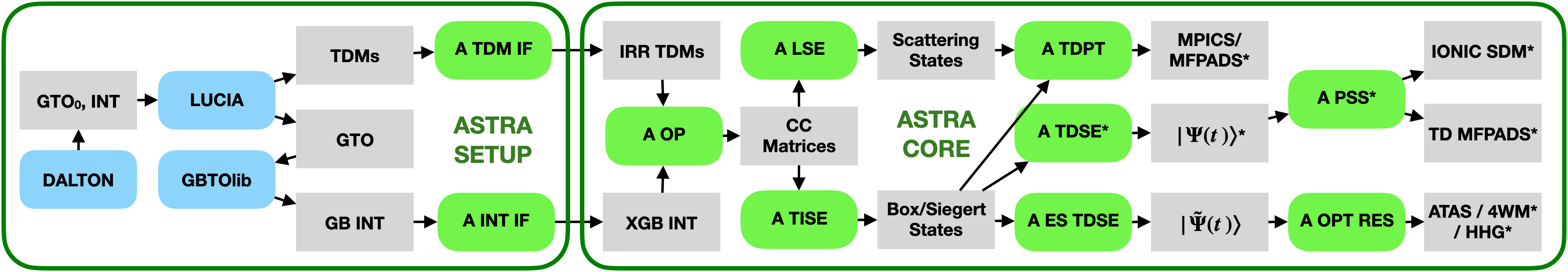
Figure 1: astra flow scheme. Rounded boxes represent executables, whereas square boxes represent databases. The “A” prefix indicates an executable from the astra suite. In the setup section (left frame), from a set of configuration files (not shown), the astra Setup script invokes, in sequence: i) dalton, to compute a starting set of GTO and their associated integrals; ii) lucia, to optimize the orbitals, to compute the correlated ionic states, as well as the TDM between them; iii) gbtolib, to compute, from the optimized orbitals, the hybrid integrals with the B-splines in the molecular region. See text for details on the steps that involve only astra components. Starred elements are currently under development.

The flow diagram in Fig. 1 illustrates how the different external and internal components of astra are connected with each other. The external components are managed by a setup script. One interface (A TDM IF) converts the TDMs generated by lucia to their reduced spin-adapted form. A second interface (A INT IF) converts the hybrid integral generated by gbtolib to the internal database of astra and complements the hybrid integrals with those involving the additional set of B-splines that extends beyond the molecular region.

The right frame of the flow diagram delimits the core section of astra. The astra operator program (A OP) generates the representation of arbitrary operators in the SACC space, starting from the reduced TDM, the hybrid integrals, and the specifics of the close-coupling configuration file (not shown). Subsequently, the astra TISE program determines the eigenstates and eigenvalues of the system with either vanishing or outgoing boundary conditions. In parallel, the Lippmann-Schwinger Equation solver (A LSE) determines the scattering states. The generalized and the confined eigenstates of the system can then be used to evaluate stationary observables, such as the one-photon total ionization cross section (see Sec. V), the photoelectron emission due to external pulses (A TDSE, A PSS), by solving the TDSE in the full CC basis, or the optical response by solving the TDSE in a reduced model space of Siegert states (A ES TDSE, A OPT RES). Due to its reliance on quantum-chemistry external tools, astra only handles molecular spatial symmetry groups that are subgroups of $D_{2h}$ Hamermesh (1989).

IV.1 CASCI ionic states and TDM

The molecular orbitals can be determined using lucia for several wave function methods: Hartree-Fock, Complete Active Space Self-Consistent Field calculations (CASSCF), and Generalized and Restricted-Active-Space SCF calculations (GASSCF and RASSCF). Molecular ionization processes start from a neutral state and lead to the production of multiple ionic states with different symmetries and multiplicities. It is therefore advantageous to optimize the orbitals so they provide a balanced representation of a set of target states with different number of electrons, multiplicities, spatial symmetry, and energy. Such optimizations go under the name of state-averaged (SA) MCSCF calculations, and lucia is capable of optimizing the orbitals for an ensemble of such states. This makes lucia a well-suited QC engine for generating the orbitals and CI-expansions that subsequently are used in the photoionization codes.

In a subsequent step, lucia computes the required TDMs between all the ionic states in the CC expansion, as well as the overlap, Hamiltonian, and dipole matrix elements between all the states obtained by augmenting these ions by any of the active orbitals. For one-electron photoionization processes, one- and two-electron density matrices are sufficient, but lucia can also calculate the three-electron TDMs required for double photoionization. The TDMs are obtained in lucia over spin-orbitals and are subsequently spin-adapted by the astra interface. The lucia code determines the TDMs from CI expansions in the Slater determinant (SD) basis. However, in order to assure that the involved states have well-defined spin of the involved states, these states are defined in terms of spin-adapted configuration state functions (CSFs). The calculations of the TDMs and the inner part of a direct CI-step are thus preceded by a transformation from the CSF to the SD basis.

The expansion of a CI-state in terms of Slater determinants is realized using the formalism of spin-strings  Knowles and Handy (1984); Olsen et al. (1988); Helgaker et al. (2000). In this formalism, a SD is expressed as an alpha-spin-string, which is an ordered product of the creation-operators for the alpha-spin-orbitals, times a beta-spin-string, which is an ordered product of creation operators for beta-spin orbitals. The use of spin-strings provides a formally simple approach that can perform the CI-optimization and the subsequent calculation of TDMs in an efficient manner. An advantage of the spin-string formalism is that the information required to determine the action of a general operator on a CI expansion is easy to determine and store. In the present implementation, only information about single-electron removal and addition from strings is determined and stored. The action of operators containing several creation or annihilation operators is constructed on the fly from the lists of one-electron removals and additions.

The TDMs are also written and computed in terms of spin-strings Olsen (2000b); Kähler and Olsen (2017). A TDM is thus written as matrix with indices defining spin-strings,

$$\rho^{BA}_{\nu,\mu}=\langle A|\mathcal{O}^{\dagger}_{\mu}\mathcal{O}_{\nu}|B\rangle.$$ (25)

By letting $\mathcal{O}$  be strings of one-, two-, and three-electron annihilation operators, the one-, two- and three-electron density matrices of Eq.(7) are obtained. The various forms of the TDMs are calculated using a common suite of routines, where the states $\mathcal{O}_{\mu}|A\rangle,\mathcal{O}_{\nu}|B\rangle$ first are determined as expansions in SDs, $|I\rangle$,

$$\mathcal{O}_{\mu}|A\rangle={\sum}_{I}C^{A}_{\mu I}|I\rangle,\quad\mathcal{O}_{\nu}|B\rangle={\sum}_{I}C^{B}_{\nu I}|I\rangle.$$ (26)

For a given state A, the dimension of $C^{A}_{\mu I}$ and the operation count for its evaluation is approximately $N^{n}N_{\mathrm{det}}$, where $N$ is the number of active orbitals, $n$ is the order of the TDM, and $N_{\mathrm{det}}$  is the number of SDs in the expansion. In a second step, the TDM is obtained by matrix multiplication,

$$\rho^{BA}_{\nu,\mu}=\langle A|\mathcal{O}^{\dagger}_{\mu}\mathcal{O}_{\nu}|B\rangle={\sum}_{I}C^{A\ast}_{\mu I}C^{B}_{\nu I}.$$ (27)

This matrix multiplication scales as $N^{2n}N_{\mathrm{det}}$. For an example with 20 active orbitals and 1 million SDs, the operation count for the evaluation of $C^{B}_{\nu I}$ for a two-electron TDM is about $4\times 10^{8}$ and the following matrix-multiplication requires about $3\times 10^{11}$ operations. In the above estimates, simplifications arising from spatial symmetry were neglected. For a molecule with $N_{\mathrm{IRR}}$ irreducible representations, the operation count the the matrix multiplication is reduced by a factor of about $N_{\mathrm{IRR}}^{2}$. On a single core of a modern CPU, the discussed TDM for a molecule with 4 irreducible representations may thus be evaluated in a few seconds.

IV.2 Orbital basis

As commented in Sec. III.2, the expressions for the CC matrix elements suggest a natural partition of the orbitals in inactive, active, virtual, and external, which helps simplify their calculation. Figure 2 illustrates schematically the different orbitals.

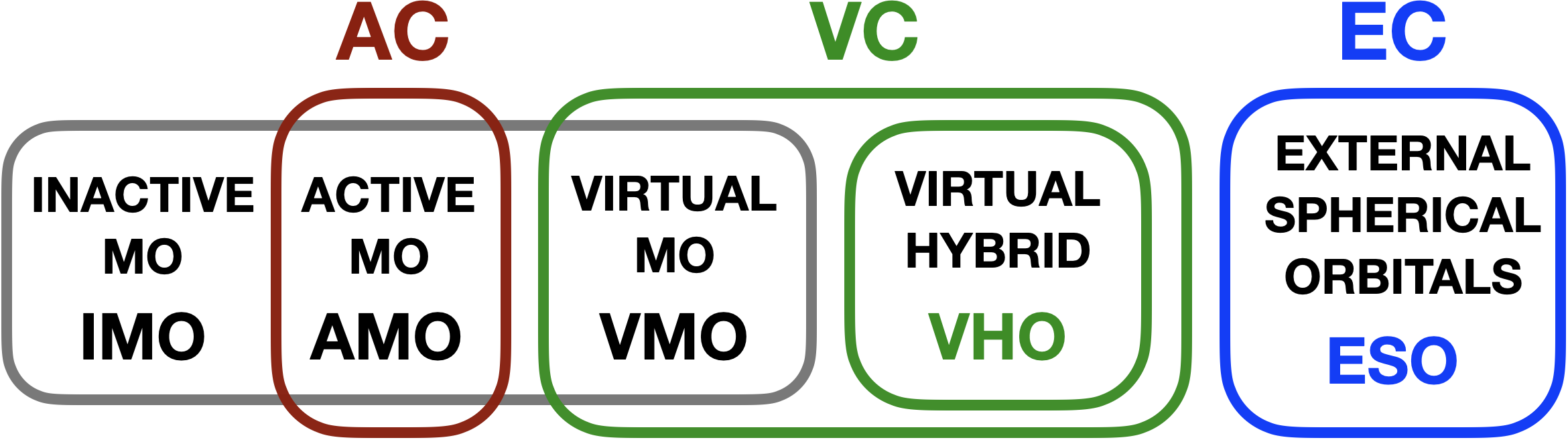
Figure 2: Schematic classification of the electronic orbitals used in astra CC expansion. The labels over the frames, AC, VC, and EC, indicate the active, virtual, and external component of the close-coupling channel obtained by augmenting a given ion by the full set of the non-inactive orbitals.

An initial set of atomic GTO orbitals are used to generate an orthonormal set of molecular orbitals (MO), $\phi^{M}_{i}$, $\langle\phi_{i}^{M}|\phi_{j}^{M}\rangle=\delta_{ij}$, optimized by means of a self-consistent-field calculation (HF, RASSCF, CASSCF, etc.). All MOs are negligible beyond a certain distance $R_{\mathrm{mol}}$ from the molecular barycenter. We call $r<R_{\mathrm{mol}}$ the molecular region. The MOs are divided in inactive orbitals (IMO), which are doubly occupied in all the ions, active orbitals (AMO), which have variable occupation numbers in the ions, and virtual orbitals (VMO), unoccupied in the ions,

$$\left\{\phi^{M}_{i}\right\}=\left\{\phi^{IM}_{i}\right\}_{i\in I_{IM}}\cup\left\{\phi^{AM}_{i}\right\}_{i\in I_{AM}}\cup\left\{\phi^{VM}_{i}\right\}_{i\in I_{VM}}$$

The MOs are assumed to be adequate to represent the correlated state of the $N-1$ electrons of the ion. However, they are normally insufficient to describe the state of an $N-$th electron in interaction with the ion, particularly for energies close to or above the ionization continuum. The virtual hybrid orbitals (VHO) are obtained by complementing the virtual MOs with a set of internal spherical B-splines Brosolo et al. (1992); Bachau et al. (2001); Marante et al. (2014), with support within the molecular region,

$$\chi^{\mathrm{int}}_{n\ell m}(\vec{r})=N_{n}r^{-1}B^{\mathrm{int}}_{n}(r)\,X_{\ell m}(\hat{r}),$$ (28)

where $X_{\ell m}(\hat{r})$ are real spherical harmonics and $N_{n}$ are normalization constants. The internal B-splines are orthonormalized to the MOs,

$$\phi^{VH}_{i}=\sum_{nm\ell}\chi^{\mathrm{int}}_{n\ell m}\,c_{nm\ell,i}+\sum_{j}\phi^{M}_{j}c_{ji},$$ (29)

$$\langle\phi^{VH}_{i}|\phi^{M}_{j}\rangle=0,\quad\langle\phi^{VH}_{i}|\phi^{VH}_{j}\rangle=\delta_{ij}.$$ (30)

This second step is carried out by gbtolib Mašín et al. (2020), by performing a Gram-Schmidt orthogonalization of the B-spline basis with the MOs (leaving the MOs unchanged) followed by a symmetric orthogonalization of the resulting set. The program also evaluates the monoelectronic and bielectronic integrals involving these hybrid orbitals.

The MOs and VHOs together afford to the CC space considerable flexibility for the description of a photoelectron subject to the polycentric field of the ion. Finally, the external spherical orbitals (ESO) are spherical B-splines that extend the internal B-spline set beyond the molecular region

$$\phi^{E}_{n\ell m}(\vec{r})=N_{n}r^{-1}\,B^{\mathrm{ext}}_{n}(r)\,X_{\ell m}(\hat{r}).$$ (31)

The MOs and the external B-splines have effectively disjoint support

$$\phi^{M}_{i}(\vec{r})\,\phi^{E}_{n\ell m}(\vec{r})\simeq 0,\quad\forall\vec{r},$$ (32)

which means that the integral of any local operator between an external B-spline and an hybrid orbital can be expressed in terms of integrals between B-spline functions only.

IV.3 Matrix elements

Taking into account the different groups of orbitals used to form the CC channels, we can further simplify the expression for the matrix elements of the different operators given in section III. The structure of the Hamiltonian matrix is schematized in Fig. (3), where the colored regions identify coupling between channels while the white areas correspond to regions with null matrix elements.

Figure 3: Block-structure of the Hamiltonian matrix between the CC states. The parts in white are empty. While the blocks are not to scale, it is clear that the matrix is highly sparse. There are essentially five different types of blocks (colored online), which correspond to as many separately optimized formulas and set of integrals: 1 for (99), 2 for (100), 3 for (101) and for 4, 5 see (102).

The evaluation of the overlap and of one-body operators is relatively simple. The most complex monoelectronic matrix elements to evaluate are those between AC states, which involves both 1B-TDM and 2B-TDM [see (14)]. Overall, however, purely monoelectronic operators are straightforward to evaluate. In this section, therefore, we will focus on the Hamiltonian only. Apart for the complex absorbing potential, which affects exclusively the diagonal blocks between external orbitals, the rest of the Hamiltonian is Hermitian. Therefore, without loss of generality, we can limit the description of the Hamiltonian matrix elements to the upper triangular set of blocks of the close-coupling matrix. The evaluation of an Hamiltonian matrix element requires the 3B-TDM only when both CC states belong to an AC. Since this matrix elements involves MOs only, it is convenient to carry out the calculation directly within lucia. astra is then left with the minimal task of evaluating, from the Hamiltonian matrix element between CC states, only those involving at least a VC or EC state, as detailed in App. C.4.

Let’s now consider the general expression (15) for the other blocks. For the active-virtual blocks (AV), the Hamiltonian is

$$\begin{split}H^{AV}_{Ap,Bq}&=\delta_{AB}\tilde{h}_{pq}+W^{BA}_{pr}\tilde{h}_{rq}\\ &+[pq|rs]Q^{BA}_{sr}+[ps|rq]W^{BA}_{sr}+[qt|rs]P^{BA}_{ps,tr},\end{split}$$

whereas the blocks between active and external states are zero, $H^{AE}_{Ap,Bq}=0$. Notice that the AV blocks are the only ones involving 2B-TDMs. Since there are comparatively few such elements, the calculation is inexpensive. For the VV block, the Hamiltonian contains both local and non-local inter-channel coupling potentials,

$$\begin{split}H^{VV}_{Ap,Bq}&=\delta_{AB}(E_{A}\delta_{pq}+\tilde{h}_{pq})+\\ &+[pq|rs]Q^{BA}_{sr}+[ps|rq]W^{BA}_{sr},\end{split}$$

whereas in the VE and EE blocks only the local potential remains (X = V, E),

$$\begin{split}H^{XE}_{Ap,Bq}=\delta_{AB}(E_{A}\delta_{pq}+\tilde{h}_{pq})+[pq|rs]Q^{BA}_{sr}.\end{split}$$ (33)

The local potential $[pq|rs]Q^{BA}_{sr}$ describes the repulsion between two disjoint distributions of charge, one confined within and one outside the molecular region, i.e., the multipolar electrostatic coupling between channels. The expression, therefore, can be conveniently rearranged by means of a multipole expansion of the electron-electron repulsion energy

$$\frac{1}{|\vec{r}-\vec{r}^{\prime}|}=\sum_{\ell m}\frac{4\pi}{2\ell+1}\frac{r_{<}^{\ell}}{r_{>}^{\ell+1}}X_{\ell m}(\hat{r})X_{\ell m}(\hat{r}^{\prime}),$$ (34)

where $X_{\ell m}(\hat{r})$ are real spherical harmonics Homeier and Steinborn (1996). The bielectronic matrix element $[pq|rs]$ then becomes,

$$[pq|rs]=\sum_{\ell m}o^{(\ell m)}_{pq}M^{(\ell m)}_{rs},$$

where

$$o^{(\ell m)}_{pq}=\langle p|\frac{X_{\ell m}(\hat{r})}{r^{\ell+1}}|q\rangle,\quad M^{(\ell m)}_{rs}=\frac{4\pi\langle r|r^{\ell}X_{\ell m}(\hat{r})|s\rangle}{2\ell+1}.$$

We can now recognize that the one-body part of the Hamiltonian $\tilde{h}_{pq}$ defined in (16) already contains a multipolar nuclear attraction potential, whose associated set of moments are given by

$$M_{\mathrm{nuc}}^{(\ell m)}=\frac{4\pi}{2\ell+1}\sum_{\alpha}^{N_{\mathrm{at}}}Z_{\alpha}R_{\alpha}^{\ell}X_{\ell m}(\hat{R}_{\alpha}).$$ (35)

It is convenient, therefore, to gather the nuclear attraction and the electronic repulsion terms in a single transition multipolar momentum $\mathcal{M}^{(\ell m)}_{AB}$, defined as,

$$\mathcal{M}^{(\ell m)}_{AB}={\sum_{rs}}^{\prime}M^{(\ell m)}_{rs}Q^{BA}_{sr}+2\sum_{x}^{\mathrm{core}}M_{xx}^{(\ell m)}-M_{\mathrm{nuc}}^{(\ell m)},$$ (36)

The monopolar momentum, of course, is simply the ionic charge, $\mathcal{M}_{AB}^{(00)}=\delta_{AB}Z_{\mathrm{ion}}$, and the expression for the Hamiltonian in the outer region given in (33) can therefore be rewritten as:

$$\begin{split}H^{XE}_{Ap,Bq}&=\delta_{AB}(s_{pq}E_{A}+t_{pq}-Z_{\mathrm{ion}}o^{(00)}_{pq})+\\ &+\sum_{\ell m}^{\ell>0}o^{(\ell m)}_{pq}\mathcal{M}^{(\ell m)}_{AB}.\end{split}$$ (37)

where $t_{pq}$ is a kinetic-energy matrix element.

V Results

This section illustrates astra performance by comparing its results with well established and independent single-ionization codes, together with experimental references, when available. We apply astra to the calculation of selected bound and resonant state parameters, and total photoionization cross section of three reference model systems: the boron atom, the nitrogen molecule, and formaldehyde, H₂CO, as a representative of an open-shell atomic system, a diatomic molecule, and a simple polyatomic molecule, respectively. The results are compared with the best values available in the literature, with which we find an excellent agreement. In the case of N₂, we consider different levels of approximation to illustrate both the consistency of the method with independent benchmark calculations, such as CIS, as well as the flexibility with which electronic correlation in ionization can be treated already within the current implementation of astra.

V.1 Boron

In this section, we discuss the computation of the bound state energies, resonance parameters, and photoionization cross-section of atomic boron and compare the results with the newstock suite of atomic photoionization codes Carette et al. (2013) as well as with a dedicated three-active-electron atomic code (taec) Argenti and Moccia (2016). Boron doublet CC space is built from ions with both singlet and triplet multiplicity. This comparison, therefore, is particularly relevant because it allows us to test the correct implementation of the TDMCC method when TDMs between states with different multiplicity are required. Although both astra and newstock use equivalent CC expansions, the two approaches are intrinsically different. newstock, as an atomic photoionization code, uses the full $SO(3)$ symmetry of the atom, whereas astra uses the $D_{2h}$ abelian point group. newstock relies on the non-relativistic multi-configuration Hartree-Fock (MCHF) program of the ATSP2K Froese Fischer et al. (2007) package to compute the parent-ion states. To obtain the equivalent degree of local electron correlation, we employ the same number of ionic states in astra and newstock calculations. The ionic states are optimized by including all possible single and double excitations from the reference determinant with active orbitals up to the principal quantum number $n=4$. taec Argenti and Moccia (2016) uses a virtually complete two-electron basis for the two active valence electrons of the B⁺ ion in the field of a polarizable core, as well as an optimized set of several thousands configurations selected from the full-CI three-active-electron space, and a significantly larger CC expansions compared with either newstock or astra. As one may expect from a dedicated program, therefore, taec results are closer to the experimental values listed in the NIST database Kramida et al. (2022).

Table 1: Comparison of the energies of the first 11 singlet and triplet bound states of B II, $E-E_{2s^{2}}$ (eV).

Conf.	astra	newstock	taec Argenti and Moccia (2016)	Exp. Kramida et al. (2022)
$2s2p$ (${}^{3}{P^{o}}$)	4.6563	4.6308	4.6391	4.6317
$2s2p$ (${}^{1}{P^{o}}$)	9.3240	9.3421	9.1187	9.1000
$2p^{2}$ (${}^{3}{P^{e}}$)	12.373	12.256	12.287	12.266
$2p^{2}$ (${}^{1}{D^{e}}$)	12.856	12.860	12.706	12.691
$2p^{2}$ (${}^{1}{S^{e}}$)	16.012	16.001	15.835	15.827
$2s3s$ (${}^{3}{S^{e}}$)	16.036	16.037	16.095	16.089
$2s3s$ (${}^{1}{S^{e}}$)	17.166	17.300	17.069	17.062
$2s3p$ (${}^{3}{P^{o}}$)	17.839	17.831	17.858	17.853
$2s3p$ (${}^{1}{P^{o}}$)	17.880	17.910	17.874	17.866
$2s3d$ (${}^{3}{D^{e}}$)	18.652	18.650	18.681	18.678
$2s3d$ (${}^{1}{D^{e}}$)	19.230	19.380	19.183	19.178

In constructing the CC expansion for astra and newstock calculations, we have included the first 12 parent ions, which are listed in Table 1. For the astra computation, the ionic Hartree-Fock orbitals are generated with dalton Aidas et al. (2014) using the aug-cc-pVQZ basis. In astra and newstock, the results of the ionic states with dominant configurations up to $2s3d(^{1}\mathrm{D^{e}})$ are compared in Table 1 relative to the $2s^{2}(^{1}\mathrm{S^{e}})$ ionic ground state. The agreement between our results and the experimental values is remarkable. The values computed with astra lie within 0.03 to 0.2 eV of the experimental values, which is deemed sufficient to ascertain the consistency of astra’s implementation. In both astra and newstock, the twelve parent ions are coupled to photoelectrons with angular momentum up to $l_{max}=3$, within a quantization box of 300 a.u., employing B-splines of order 7 and node separation of 0.3 a.u. In astra, $R_{\mathrm{mol}}=20$ a.u. and a single CAP is used, which starts at $R_{\alpha}=200$ a.u.

Table 2: Bound state energies of B I, $E-E_{2s^{2}2p}$ (eV).

Conf.	astra	newstock	taec Argenti and Moccia (2016)	Exp. Kramida et al. (2022)
$2s2p^{2}$ (${}^{4}\mathrm{P^{e}}$)	3.584	3.564		3.552
$2s^{2}3s$ (${}^{2}{S^{e}}$)	4.869	4.881	4.958	4.964
$2s2p^{2}$ (${}^{2}{D^{e}}$)	5.916	5.927	5.939	5.933
$2s^{2}3p$ (${}^{2}{P^{o}}$)	5.993	5.990	6.021	6.027
$2s^{2}3d$ (${}^{2}{D^{e}}$)	6.707	6.682	6.785	6.790

Table 2 lists the first few bound-state energies of B I with doublet and quartet symmetries. For the $2s^{2}2p(^{2}P^{o})$ ground state, the absolute value of energy obtained from astra is -24.600 14 a.u. which differs from more accurate non-relativistic MCHF calculations Froese Fischer et al. (2013) by 0.0538 a.u. This energy difference is commensurate with the value of 0.044 735 a.u estimated for the K-shell correlation energy Davidson et al. (1991), which is not accounted for in the present calculation. The residual discrepancy is compatible with the larger active space used in the MCHF calculation.

Table 3: Comparison of effective quantum number, $n^{*}$ and resonance width $\Gamma$ (a.u.), of ${}^{2}{P^{o}}$ resonances between $2s^{2}$ and $2s2p(^{3}{P^{o})}$ thresholds. The notation 5.94[-3] stands for $5.94\times 10^{-3}$.

	astra		newstock		taec Argenti and Moccia (2016)
Conf.	$n^{*}$	$\Gamma$	$n^{*}$	$\Gamma$	$n^{*}$	$\Gamma$
$2s2p3s$	2.146	5.94[-3]	2.131	5.58[-3]	2.140	5.73[-3]
$2s2p4s$	3.120	1.79[-3]	3.157	1.63[-3]	3.157	1.59[-3]
$2s2p5s$	4.170	6.98[-4]	4.164	6.96[-4]	4.161	6.69[-4]
$2s2p6s$	5.172	3.59[-4]	5.166	3.60[-4]	5.162	3.44[-4]
$2s2p7s$	6.173	2.10[-4]	6.167	2.10[-4]	6.163	2.00[-4]

Table 4: Comparison of effective quantum number, $n^{*}$ and resonance width $\Gamma$ (a.u.), of ${}^{2}{S^{e}}$ resonances between $2s^{2}$ and $2s2p(^{3}{P^{o}})$ thresholds.

	astra		newstock		taec Argenti and Moccia (2016)
Conf.	$n^{*}$	$\Gamma$	$n^{*}$	$\Gamma$	$n^{*}$	$\Gamma$
$2s2p3p$	2.765	4.99[-4]	2.743	5.22[-4]	2.733	4.70[-4]
$2s2p4p$	3.767	1.81[-4]	3.754	1.89[-4]	3.736	1.67[-4]
$2s2p5p$	4.766	8.51[-5]	4.756	8.96[-5]	4.736	7.75[-5]
$2s2p6p$	5.765	4.67[-5]	5.756	4.93[-5]	5.736	4.21[-5]
$2s2p7p$	6.765	3.15[-5]	6.756	2.99[-5]	6.735	2.54[-5]

Table 5: Comparison of effective quantum number, $n^{*}$ and resonance width $\Gamma$ (a.u.), of ${}^{2}{D^{e}}$ resonances between $2s^{2}$ and $2s2p(^{3}{P^{o}})$ thresholds.

	astra		newstock		taec Argenti and Moccia (2016)
Conf.	$n^{*}$	$\Gamma$	$n^{*}$	$\Gamma$	$n^{*}$	$\Gamma$
$2s2p3p$	2.581	1.95[-3]	2.579	1.88[-3]	2.568	1.74[-3]
$2s2p4p$	3.596	6.75[-4]	3.594	6.46[-4]	3.585	5.68[-4]
$2s2p5p$	4.601	3.12[-4]	4.599	2.98[-4]	4.585	2.87[-4]
$2s2p6p$	5.601	1.70[-4]	5.601	1.62[-4]	5.588	1.54[-4]
$2s2p7p$	6.603	1.06[-4]	6.601	9.77[-5]	6.588	9.34[-5]
$2s2p4f$	4.013	1.56[-7]	4.013	1.07[-7]	4.009	1.57[-7]
$2s2p5f$	5.012	1.37[-7]	5.012	9.73[-8]	5.009	1.19[-7]
$2s2p6f$	6.012	1.32[-7]	6.011	7.27[-8]	6.008	8.65[-8]

In astra, the resonance parameters are obtained by diagonalizing the multi-channel CC Hamiltonian in the presence of a CAP, whereas newstock enforces outgoing boundary conditions using exterior-complex scaling (ECS) Simon (1979); Lindroth (1995); McCurdy and Martín (2004). Table 3 compares the effective quantum number, $n^{*}=[2(E_{thr}-E_{n})]^{-1/2}$, and resonance width, $\Gamma$, of selected autoionizing states with ${}^{2}P^{o}$ symmetry, between the the $2s^{2}(^{1}{S^{e}})$ and $2s2p(^{3}{P^{o}})$ B⁺ thresholds. The results for the dominant $2s2p(^{3}{P^{o}})ns$ series from astra are in excellent agreement with those obtained with newstock and taec. Table 4 shows the parameters for the first few terms of the $2s2p(^{3}{P^{o}})np\,({{}^{2}S^{e}})$ autoionizing states. The resonance parameters for the two main series, $2s2p(^{3}{P^{o}})np$ and $2s2p(^{3}{P^{o}})nf$ of ${}^{2}{D^{e}}$ autoionizing states are listed in Table 5.

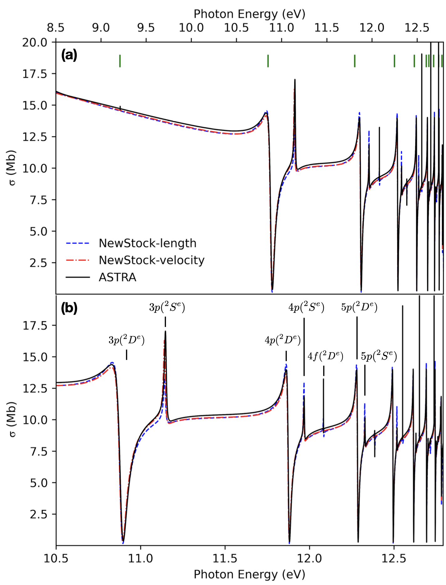
Figure 4: (Color online) (a) Total photoionization cross-section between the $2s^{2}(^{1}S^{e})$ and $2s2p({{}^{3}P^{o}})$ thresholds, from ${{}^{2}P^{o}}$ ground state of atomic boron, computed with astra (solid black line) and compared with the length (dashed blue line) and the velocity (dash-dotted red line) gauge results from newstock. The solid green lines indicate the positions of the bound states of ${}^{2}P^{e}$ symmetry. (b) Same cross-section as in the top panel, magnified in the resonant region, which exhibits autoionizing states with both ${}^{2}S^{e}$ and ${}^{2}D^{e}$ symmetry. The notation $n\ell(^{2}L^{e})$ denotes a resonance with dominant configuration $2s2pn\ell$ coupled to ${}^{2}L^{e}$ symmetry.

Figure 4 compares the total photoionization cross-section of boron, from the ${}^{2}{P^{o}}$ ground state to the energy region between the $2s^{2}$ and the $2s2p$ B⁺ thresholds, computed in the length gauge with astra, with the one computed with newstock, both in length and in velocity gauge. As discussed in Sec. III, in this work, astra evaluates the total cross section using the optical theorem (24), whereas the cross section in newstock is computed from the dipole transition matrix elements between the ground state and a complete set of scattering states of the atom. The two calculations, which differ entirely in their methodology, are in remarkable agreement with each other. In particular, astra accurately reproduces the characteristic asymmetry of the multi-channel resonant profiles of the many autoionizing states in this region.

Figure 4a covers the whole energy interval between the first and second threshold. Figure 4b shows a close up on the resonant region, and identifies selected terms in the three main resonant series. The broad $2s2pnp$ $({{}^{2}D^{e}})$ and the narrow $2s2p3p(^{2}S^{e})$ series dominate the total cross section. A much narrower $2s2pnf(^{2}D^{e})$ series is visible near the second ionization threshold. As shown in Fig. 4a, the boron spectrum computed with astra exhibits a few additional ultra-narrow resonant features, highlighted by vertical tics (green online), that deserve some comments. By comparing the positions of the Rydberg bound states in newstock and astra, it can be shown that this series corresponds to ${}^{2}P^{e}$ bound states. These bound states manifest themselves as vanishingly narrow resonances in the photoionization spectrum due to the miniscule coupling of the ${}^{2}P^{e}$ bound states to the ${}^{2}D^{e}$ continuum. Similar minor symmetry mixing are to be expected in a molecular code because, in $D_{2h}$ symmetry, the distinction between some $SO(3)$ irreducible representations is enforced dynamically, through numerical cancellations, rather than geometrically. That said, the mixing is small indeed. The largest of these resonances, at $\sim 9.2$ eV, has a width of just $\approx 10^{-13}$ a.u., comparable to machine precision, whith the higher terms of the series being narrower still. Far from representing a failure of the code, therefore, such small values testify the remarkable accuracy with which astra does reproduce the spherical symmetry of the atom.

The agreement between the two different ab-initio approaches shows that the astra formalism, based on non-standard high-order TDMs between ionic states with different multiplicities and designed for molecular systems, is consistent and can be used to obtain accurate results for atoms Puskar et al. (2023) as well.

V.2 Nitrogen Molecule

The nitrogen molecule is an ideal system to test the accuracy of states in the ionization continuum, thanks to the availability of several theoretical and experimental benchmarks in the literature. In this subsection, we report on several comparisons, within the fixed-nuclei approximation (FNA). First, we ascertain that, to the minimal CIS level, astra exactly reproduces the same result as an independent ad hoc CIS code, as it should. Next, we test astra consistency and performance with the CC space constructed from correlated ions by comparing our results with those obtained with xchem Marante et al. (2017b), a state-of-the art molecular-ionization code, as well as with experimental values.

V.2.1 Comparison with ad hoc CIS Code

The astra suite has been benchmarked against an ad hoc CIS code for the N₂ molecule, described in App. D. In the CIS model, the ionic states for the CC expansion are obtained by creating a vacancy in any of the valence orbitals of the Hartree-Fock determinant of the N₂ ground state. All these single-configuration ions are subsequently coupled to all available VMOs and VHOs. The CC space obtained with this approach, therefore, coincides with the CIS space from the HF ground state of N₂. The HF ground state was computed using a 6-31G basis, whereas for the hybrid orbitals we used B-splines of order 6, with a node separation of 0.77 a.u. and angular momentum $\ell\leq 2$, within a 20 a.u. quantization box. The formulas for the transition-density matrices in the CIS basis, and the CC matrix elements of the Hamiltonian and the dipole operators, are particularly simple, as shown in App. D. The density matrices were used to test, in the CIS case, the consistency of the TDMs generated by lucia, as well as that of the spin-adapted reduced TDMs evaluated by astra. The matrix elements of the Hamiltonian, computed separately by the CIS code, were used to ascertain the correctness of the astra structure code. The singlet states energy obtained from the Hamiltonian diagonalization in astra agree with those computed with the CIS code within $10^{-12}$ a.u., which is compatible with the propagation of error entailed by the necessary operations, executed with machine precision.

V.2.2 Comparison with xchem in CI-singles subspace

astra accounts for the matrix elements between poly-centric GTOs and B-splines, as well as for the exchange terms between hybrid and ionic orbitals. This feature allows us to use B-splines across the whole radial range, thus providing the flexibility necessary to achieve the large photoelectron energies typical of core spectroscopies (several hundreds eV) as well as to describe the continuum of comparatively large molecules.

As detailed in the previous section, we ascertained that astra predictions coincide with those of an ad-hoc CIS code, when the same hybrid integrals are used. In the present section, we show that, in the CIS case, the results generated by astra are compatible with those computed with xchem, an independent and well established suite of molecular photoionization codes. Like astra, xchem is based on the CC ansatz and on the use of Gaussian-B-spline hybrid functions Marante et al. (2017a, b); Klinker et al. (2018c, a); Borràs et al. (2021). In contrast with astra, however, xchem employs a different algorithm to evaluate CC matrix elements, and it confines B-splines beyond a certain distance $R_{0}$ to limit their overlap with the ionic poly-centric GTOs. In xchem, the molecular and the external regions are bridged by a diffuse set of monocentric GTOs $G_{i\ell k}(r)=r^{\ell+2k}\exp{(-\alpha_{i}r^{2})}$ Marante et al. (2014).

Table 6 compares the energy of the N₂ ground state and of the first few excited singlet states, as well as the dipole oscillator strengths from the former to the latter, obtained by diagonalizing the CC Hamiltonian computed either with xchem, using the 6-31G basis, or with astra, using the 6-31G and the larger cc-pVQZ basis. In all these cases, the CC expansion includes the $X\phantom{A}\!\!\!^{2}\Sigma_{g}^{+}$, $A\phantom{A}\!\!\!^{2}\Pi_{u}$ and $B\phantom{A}\!\!\!^{2}\Sigma_{u}^{+}$ parent ions, augmented by single-electron states with $\ell\leq 2$, in a 400 a.u. quantization box. The ions were confined to a sphere with radius $R_{\mathrm{mol}}=20$ a.u. and two CAP were employed, starting at 100 and 200 a.u. with a strength of $10^{-6}$ and $10^{-5}$, respectively. The ionic states are obtained from the HF configuration by removing one electron from the $3\sigma_{g}$, $1\pi_{u}$, and $2\sigma_{u}$ orbitals. The B-splines were of order 8, the node separation chosen as $\Delta r=0.5$ a.u. and for the diffuse GTOs in xchem we followed the same even-tempered set of exponents $\alpha_{i}$ defined in Klinker et al. (2018a), with $k=2$. The nitrogen molecule is aligned along the $\hat{z}$ axis and the internuclear distance is set to the experimental equilibrium value $R=1.098$ Å Huber and Herzberg (1979).

Table 6: Energy of and dipole oscillator strength (OS) between the ground state and the first few bright states of $\mathrm{N_{2}}$, computed with xchem and astra in the CI-singles limit, using a 6-31G basis for the HF orbitals. The energies are relative to astra ground state.

	Energy (eV)		OS (a.u.)
State	xchem	astra	xchem	astra
$X\,{{}^{1}\mathrm{\Sigma_{g}^{+}}}$	00.004	00.000	-	-
$1\,\,{{}^{1}\mathrm{\Pi_{u}^{\phantom{+}}}}$	15.236	15.236	0.2062	0.2066
$1\,\,{{}^{1}\mathrm{\Sigma_{u}^{+}}}$	16.267	16.287	0.2053	0.2098
$2\,\,{{}^{1}\mathrm{\Pi_{u}^{\phantom{+}}}}$	16.311	16.321	0.0812	0.0802

The energies computed with xchem and astra using the 6-31G basis differ by no more than 0.02 eV, which is a remarkable agreement, given how different the virtual monoelectronic orbitals in the molecular region are for these two methods. The oscillator strength is more sensitive to the quality of the underlying electronic numerical basis. Nevertheless, astra’s results do not deviate more than 1% from those of xchem.

In Fig. 5, we compare the quantum defect $\mu_{n}\equiv n-n^{*}$ of four Rydberg series converging to the first ionization threshold, $X\,{{}^{2}\Sigma_{g}^{+}}$. The quantum defects obtained with the two methods are within $0.5\%$ for all values of $n^{*}$.

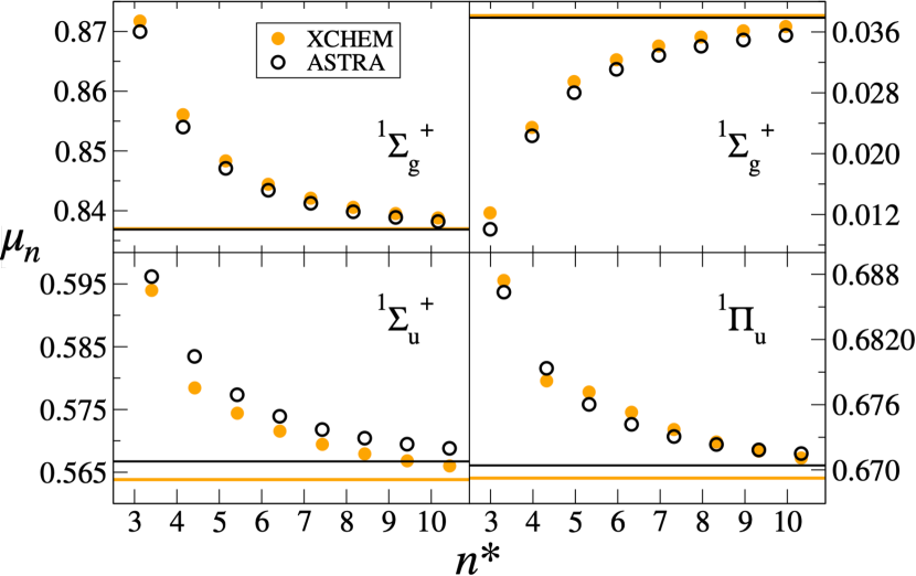
Figure 5: Quantum defect $\mu_{n}^{\Gamma}$ vs the effective principal quantum number $n^{*}$ for four Rydberg series of bound states in three symmetries, computed with xchem (filled circles, yellow online) and astra (black empty circles) within the same CI-singles CC space used in Table 6. Horizontal lines indicate $\mu_{\infty}^{\Gamma}=\lim_{n\to\infty}\mu_{n}^{\Gamma}$.

The agreement, therefore, is not restricted to the first few bound states, which may be well represented by GTOs alone, but it extends to Rydberg states with large quantum numbers and with a radial size well beyond the molecular region. These positive comparisons shows that, for the present calculation: i) the two different configuration spaces made available to the $N$-th electron in xchem and astra are equivalent, and ii) astra correctly employs the gbtolib hybrid basic integrals.

V.2.3 CC with correlated ions

In this section, we go beyond the CIS approximation by considering the CC expansion obtained from the $X\,{\Sigma_{g}^{+}}$, $A\,{{}^{2}\Pi_{u}}$ and $B\,{{}^{2}\Sigma_{u}^{+}}$ correlated ions augmented by virtual orbitals with asymptotic angular momentum up to $\ell_{max}=3$. The ions are computed by means of a CASCI calculation Helgaker et al. (2000), over the $\{2\sigma_{g/u},3\sigma_{g/u},1\pi_{u},1\pi_{g}\}$ set of active orbitals, keeping the core $1\sigma_{g/u}$ orbitals inactive (doubly occupied), and employing three different GTO bases: 6-31G, cc-pVDZ, and cc-pVTZ. Table 7 compares the energies of the first five singlet bound states obtained with astra in the three different bases, alongside those obtained with xchem in the minimal 6-31G basis. All the energies are relative to the ground state obtained with astra with the cc-pVTZ basis. For the xchem calculations, the same active space defined for astra is employed to perform a CASCI and obtain the correlated ionic states. The same basis of diffused GTOs utilized in the CIS calculations is used to complement the polycentric GTOs at short range. Once again, the agreement between xchem and astra is excellent.

Table 7: Energy of the first five singlet states of $\mathrm{N_{2}}$, in eV, obtained by including correlated parent ions in the CC (see text for details) and using different GTO basis. The energy values are with respect to the astra ground state when the basis set used to generate the molecular orbitals is cc-pVTZ.

	xchem	astra
State	6-31G	6-31G	cc-pVDZ	cc-pVTZ
$1\,\,{{}^{1}\mathrm{\Sigma_{g}^{+}}}$	0.639	0.631	0.128	0.000
$1\,\,{{}^{1}\mathrm{\Pi_{g}^{\phantom{+}}}}$	12.890	12.889	10.841	10.219
$1\,\,{{}^{1}\mathrm{\Sigma_{u}^{-}}}$	13.142	13.138	11.078	10.467
$2\,\,{{}^{1}\mathrm{\Sigma_{g}^{+}}}$	15.051	15.051	13.038	12.784
$1\,\,{{}^{1}\mathrm{\Delta_{u}^{\phantom{+}}}}$	15.636	15.639	13.622	13.411

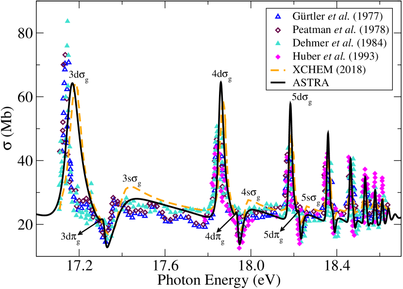
Figure 6: (Color online) Total photoionization cross section of N₂ in the Hopfield resonances region. The spectrum computed with astra (solid black line) is compared with four independent measurements (triangles and diamonds) Gürtler et al. (1977); Peatman et al. (1978); Dehmer et al. (1984); Huber et al. (1993) and another theoretical spectrum obtained with xchem (dashed line) Klinker et al. (2018a).

In the present implementation, the CC expansion only consists of correlated ionic states augmented with an extra electron either in a bound or unbound orbital. A truncated CC expansion may be insufficient to accurately reproduce all the resonant states in the energy region of interest. This is because, in the CC expansion, the response of the ionic bound electrons to an additional electron is described only in terms of the expansion on a small set of states. While the CC captures well the polarization of the ion when the additional electron is located at several Bohr radii from the nucleus, it cannot describe well dynamic correlation at short-range, such as the Coulomb hole Süle et al. (1995), which has components in the multiple-ionization states of the ion itself. A standard way of dealing with this deficiency of the CC approach is to extend the expansion to include a pseudo-channel with a large number of $N$-electron configurations built out of localized orbitals, without constraining $N-1$ electrons to any specific set of eigenstates of the ionic Hamiltonian. This pseudo channel, which is sometimes referred to as the $\mathcal{Q}$ space Feshbach (1962), can be very large. The ck-mesa code Douguet et al. (2018) has an efficient way of including the $\mathcal{Q}$ space via an optical potential built entirely out of GTOs P. Saxe, B. H. Lengsfield, R. Martin and Page (1990). xchem can also account for the $\mathcal{Q}$ space, even if it does so explicitly, which is more demanding than via an optical potential Douguet et al. (2018). The inclusion of the $\mathcal{Q}$ space in astra is outside the scope of the present work. One viable approach to circumvent this limitation is extending the CC expansion so to include closed ionization channels whose parent ions are augmented only by AMO, VMO, and VHO, and in which the extra parent ions do not have to accurately reproduce any eigenstates of the ion.

We followed this approach to reproduce the high-resolution synchrotron radiation photoionization spectrum of N₂, in the vicinity of the Hopfield series of autoionizing states Klinker et al. (2018a). Besides the three parent ions $X\phantom{A}\!\!\!^{2}\Sigma_{g}^{+}$, $A\phantom{A}\!\!\!^{2}\Pi_{u}$ and $B\phantom{A}\!\!\!^{2}\Sigma_{u}^{+}$ we have used in the previous calculations, we added another 15 to the CC: $2\phantom{A}\!\!\!^{2}\Sigma_{g}^{+}$, $1\phantom{A}\!\!\!^{2}\Sigma_{g}^{-}$, ${\operatorname{1-2}}\phantom{A}\!\!\!^{2}\Delta_{g}$, $1\phantom{A}\!\!\!^{2}\Phi_{g}$, ${\operatorname{2-4}}\phantom{A}\!\!\!^{2}\Pi_{u}$, $2\phantom{A}\!\!\!^{2}\Sigma_{u}^{+}$, ${\operatorname{1-2}}\phantom{A}\!\!\!^{2}\Delta_{u}$, ${\operatorname{1-3}}\phantom{A}\!\!\!^{2}\Pi_{g}$ and $1\phantom{A}\!\!\!^{2}\Sigma_{u}^{-}$, to define the close ionization channels. In Fig. 6 we show the comparison of the photoionization cross section computed with astra, the xchem result reported in Klinker et al. (2018a) alongside four experimental spectra Gürtler et al. (1977); Peatman et al. (1978); Dehmer et al. (1984); Huber et al. (1993). The theoretical signals have been convoluted with a 0.015 eV width normalized Gaussian to account for the experimental resolution. In the photoionization spectrum we can distinguish the three Hopfield series of resonances converging to the $B\phantom{A}\!\!\!^{2}\Sigma_{u}^{+}$ ionization threshold: $ns\sigma_{g}$, $nd\sigma_{g}$ and $nd\pi_{g}$, for which we indicate the first three terms. The astra result is in very good agreement with both the xchem calculation and with the experimental spectra. For the first resonant feature corresponding to $3d\sigma_{g}$, both theoretical the results show a broader peak than the measured value, which is likely due to residual electronic correlation missing in the early terms of the Rydberg series.

The size of the close-coupling space, in this case, is 16418 for the $A_{g}$ $D_{2h}$ symmetry, and 10918 for all the other $D_{2h}$ symmetries considered. The calculations were conducted on a standalone workstation equipped with two 2.8GHz Intel Xeon Platinum-8362 processors (32 cores each). While the current implementation of astra is serial, lapack Anderson et al. (1999) diagonalization routines employ multithreaded drivers that occupied, on average, between 17 and 19 cores. The calculation of the CC matrix elements for all the operators, the full diagonalization of the real and complex Hamiltonian and the calculation of the photoionization cross section took $\sim$2 hours.

V.3 Formaldehyde

To test astra on a non-linear polyatomic molecule, we selected formaldehyde, H₂CO, for which resonably accurate experimental Cooper et al. (1996); Tanaka et al. (2017) and theoretical Cacelli et al. (2001) photoionization cross sections are available. As for N₂, we used the FNA at the equilibrium geometry: $R_{\mathrm{CO}}=1.21$ Å, $R_{\mathrm{CH}}=1.12$ Å, $\measuredangle\mathrm{HCH}=116.5^{\mathrm{o}}$ Wang et al. (2022); Gurvich et al. (1989). As detailed below, we conducted calculations with astra at several levels of accuracy. In our largest calculation, the molecular orbitals are optimized by a state average MCSCF calculation on the first ten neutral state of the molecule, the VHO and ESO orbitals are computed with $\ell\leq 4$, and the CC expansion includes the first 37 molecular ions. The first ten ions are augmented with the full set of internal and external orbitals (AMO, VMO, VHO, and ESO), whereas the remaining 27 ions, which are all closed in the energy region of interest, are augmented by the internal orbitals only (AMO, VMO, and VHO).

Figure 7 compares the photoionization cross section of formaldehyde computed with astra between 11 eV and 22 eV, using the highest level of electronic correlation described above, with Cacelli et al. RPA calculation Cacelli et al. (2001), and with two measurements: one from a lower-resolution 1996 experiment by Cooper et al. Cooper et al. (1996) and the other from a higher-resolution 2017 experiment by Tanaka et al. Tanaka et al. (2017).

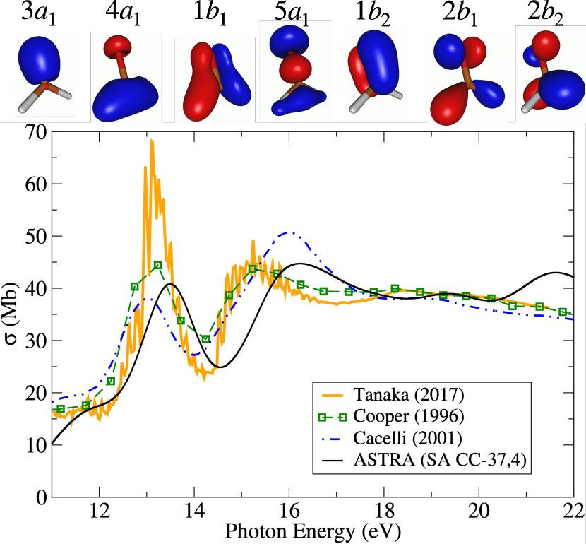
Figure 7: (Color online) Formaldehyde total photoionization cross section above the ionization threshold. The astra result (black-solid line) is obtained by including 37 ions in the CC expansion with $\ell\leq 4$. The ions were obtained through a CASCI using the orbitals coming from a SA-MCSCF calculation (see text for details). The astra sepctrum is compared with the RPA calculation in Cacelli et al. (2001) (dotted-dash line) and two measurements, with lower (dashed line and squares) and higher spectral resolution (orange-solid line) Cooper et al. (1996); Tanaka et al. (2017). The top of the figure shows the first seven molecular orbitals included in the astra active space, in ascending energy order, up to the LUMO ($2b_{2}$) Schaftenaar and Noordik (2000); Schaftenaar et al. (2017).

The spectrum exhibits two prominent shape resonances, a narrower one near 13 eV, and a broader less pronounced one at 15 eV. In the higher-resolution experiment by Tanaka, the first peak has smaller width and larger height. Considering the different resolutions, however, the results of the two experiments are compatible with each other. The results from astra are convoluted with a 1.2 eV Gaussian window, the same as in Cacelli et al. (2001), in line with the $\approx 5\%$ resolution reported by Cooper Cooper et al. (1996). The RPA calculation Cacelli et al. (2001) predicts well the position of the first peak, which it underestimates by just $0.2$ eV, while it overestimates the position of the second peak by about 1 eV. Furthermore, the height of the first and second peak are significantly under- and over-estimated, respectively. These results suggest that both resonances are highly sensitive to correlation. In the astra results, the position of the first peak is overestimated by about 0.2 eV, but its magnitude is in better agreement with the experiment by Cooper. Similarly to Cacelli’s result, the position of the second peak predicted by astra is about 1 eV above the experimental value. The peak height, however, is almost coincident with one observed in the experiment.

The results obtained with astra are arguably the ones in best agreement with the experiment, to date. However, they also suggest that the theoretical model used here is still incomplete. Two possible causes for the discrepancy with the experiment are the residual dynamic correlation not captured by the CC expansion, and the fixed-nuclei approximation, which prevents us from accounting for the effects of nuclear motion and rearrangement in the molecular ion. On the electronic-structure side, ideally, the CC expansion should include a flexible and large pseudo-channel formed by arbitrary localized configurations. On the nuclear side, one should treat consistently nuclear motion and nuclear rearrangement on multiple excited electronic potential energy surfaces in a molecule with several degrees of freedom. While we plan to tackle both of these challenges in the future, these are formidable tasks beyond the scope of the present work.

To illustrate the effect of the CC basis on formaldehyde photoionization cross-section, within the current capabilities of astra, in Fig. 8 we compare the results obtained with seven different calculations, carried out with progressively more demanding parameters.

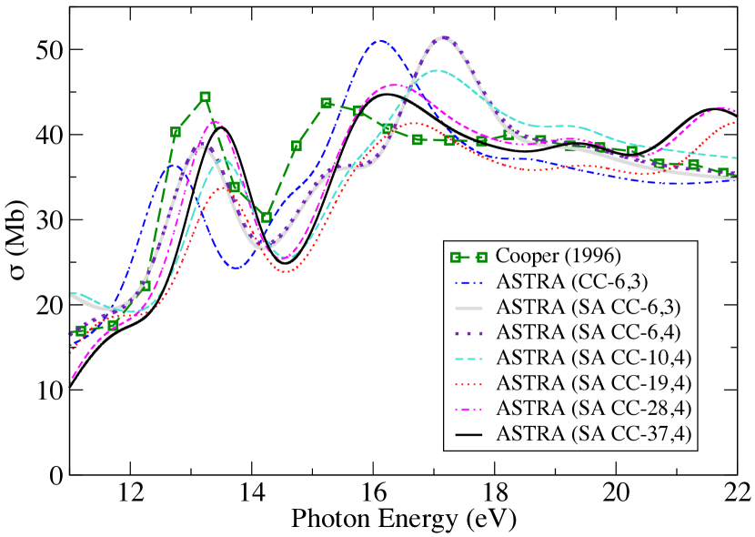
Figure 8: (Color online) Formaldehyde total photoionization cross section above the ionization threshold. Seven astra spectra are shown together with Cooper’s experiment ($\Delta E\approx 1.2$ eV) Cooper et al. (1996). Six of the astra calculations employed the same SA-MCSCF orbitals to perform the CASCI for the ionic states and they differ in the number of ions included in the CC expansion and in the maximum angular momentum considered for the partial waves. The format SA CC-N,L means that the calculation was performed by using the SA orbitals and a CC expansion with N ions and $\ell\leq L$.

In the first calculation, the CC expansion comprises six ionic states, ${\operatorname{1-2}}\!\!\!\phantom{A}^{2}B_{1}$, $1\!\!\!\phantom{A}^{2}B_{2}$, ${\operatorname{1-3}}\!\!\!\phantom{A}^{2}A_{1}$, obtained from a CASCI calculation of 12 electrons in the 9 active orbitals, $\{3a_{1},4a_{1},1b_{1},5a_{1},1b_{2},2b_{1},2b_{2},6a_{1},3b_{1}\}$, whereas the two core orbitals $1a_{1}$ and $2a_{1}$ (corresponding to the O$1s$ and C$1s$ K shells) were doubly occupied. These orbitals are obtained from the HF calculation of the neutral molecule within the cc-PVTZ GTO basis. To build the CC channels, each of these ions was augmented by an electron in any of the GTO (AMO, in the notation of Sec. III) and hybrid orbitals (VHO), and B-splines with asymptotic angular momentum $\ell\leq 3$ spanning the whole quantization box (ESO). The B-spline and $V_{\textsc{CAP}}$ parameters coincide with those used for nitrogen.

This first astra calculation reproduces the characteristic double-hump structure of the spectrum and it is in very good agreement with the results by Cacelli et al. Cacelli et al. (2001). In particular, the absolute magnitude of the two peaks in the two independent calculations are remarkably similar. Both theoretical calculations, however, underestimate the position and magnitude of the first peak, and overestimate the energy and magnitude of the second peak, compared with the experiment.

In the other six astra calculations, the molecular GTO orbitals are optimized through a SA-MCSCF step over the first 10 neutral states, with equal weights. The ions are subsequently determined by a CASCI calculation with the same number and type of inactive and active orbitals as in the first case.

In the second calculation, the CC space is generated from the first six ionic states only, augmented with orbitals with $\ell\leq 3$. The first and the second calculation, therefore, differ only in the optimization of the ion orbitals. The calculation reproduces very well the position of the first peak, quite possibly a coincidence, whereas the second peak splits into a shoulder around the position of the peak observed in the experiment and in a prominent third peak around 17 eV, with no correspondence in the measured data.

In the third calculation, the ions in the CC expansion coincide with those in the second calculation, but all the ions are now augmented with orbitals with $\ell\leq 4$. The second and the third calculation, therefore, differ only in the photoelectron partial-wave expansion. Both photoionization cross sections are almost identical except in the energy region approaching the ionization threshold ($E<12$ eV), which indicates that in the region of interest, the partial wave expansion is close to convergence for $\ell\leq 4$.

The fourth calculation coincides with the third, except that the CC expansion is extended to include the first 10 ions, each augmented by both the internal (AMO, VMO, and VHO) and by the external (ESO) partial-wave orbitals. The shoulder observed in the two previous spectra is greatly reduced and the magnitude of the second peak decreases, being closer to the experiment. The position of the first peak gets shifted 0.2 eV to higher energies and it’s magnitude decreases by 2 Mb.

In the remaining three calculations, we investigated the convergence of the cross section using the same number of fully-augmented partial-wave channels as in the fourth, but adding 9, 18, and 27 other ions to the CC expansion, each augmented by the internal orbitals only. Since the corresponding channels are all closed in the energy region of interest, these last three calculations include progressively more dynamic correlation. Going from 10 to 19 to 28 ions, the position of the second peak is lowered by almost 1 eV. The position of the first peak is only marginally affected. The inclusion of nine other ions, from 28 to 37, has a comparatively small effect, which suggests that these calculations are close to convergence for the present choice of orbitals.

VI Conclusions and Perspectives

We have described a transition-density-matrix approach to the close-coupling method (TDMCC) for molecular photoionization, implemented in the astra code, and used it to compute the bound-state parameters, autoionizing-state parameters, and the single-photon integral photoionization cross section of benchmark atomic and molecular systems. The TDMCC method scales well with the size of the CI space of the parent ion, and it delivers results in excellent agreement with those in the literature.

In future works, we will explore the scalability of astra by studying the ionization process in increasingly larger systems. Preliminary calculations indicate that ASTRA is capable of simulating the ionization of molecules as large as metallo-porphyrines, organometallic compounds comprised of $37$ or more atoms, which opens a new way to the detailed predictions of wave-function-based methods for the ionization of molecules of biological interest.

From the methodological point of view, the astra program has several natural directions along which to evolve. First, is the calculation of multichannel scattering states, which will allow us to determine photoelectron angular distributions Wu et al. (2011); Dowek and Decleva (2022), either in stationary regime, or as a result of the interaction of a target molecule with an ultrashort pulse of radiation. Second, is the extension of the calculation of the ionic states and of their TDMs from the present CASCI level to the more general RASCI Malmqvist et al. (1990); Lischka et al. (2018); Zhou et al. (2019); Casanova (2022) level. This extension will be particularly useful to describe highly conjugated systems. Third, we plan to use the SACC space as the basis for the time-dependent description of the photoionization wavepackets generated by the interaction of a target molecule with a sequence of ultrashort ionizing pulses Harkema et al. (2021); Leshchenko et al. (2023); Borràs et al. (2021). This direction will allow us to reproduce transient-absorption spectra Kobayashi et al. (2019); Kraus et al. (2018); Zin (2021); Rebholz et al. (2021), four-wave mixing spectra Cao et al. (2018); Warrick et al. (2018); Fidler et al. (2022), and photoelectron spectra Schuurman and Blanchet (2022) for state-of-the-art experiments.

In the longer term, we plan to explore also the many other natural extensions of the TDMCC formalism of astra, such as the inclusion of a Q-space for the accurate description of short-range correlation Schneider et al. (1991), the inclusion of double-escape channels Zhaunerchyk et al. (2015); Mucke et al. (2015); Lablanquie et al. (2016), to reproduce molecular double-ionization processes, as well as the description of multi-fragment systems Murillo-Sánchez et al. (2018); Lee et al. (2021); Allum et al. (2022); Howard et al. (2023); Rolles (2023) (e.g., a dissociating molecule, or a loosely bound aggregate) in terms of the TDMs of its separated components, in which the TDMs of the whole aggregate naturally factorizes, thus leading to drastic reduction in computational cost.

Appendix A Second-quantization formalism

In this section we summarize the correspondence between antisymmetric electronic functions in the first-quantization coordinate representation and the associated Fock space, as well as some basic properties of many-body operators in second-quantization (SQ). For a general description of the SQ formalism, we refer the reader to the first chapter in Helgaker et al. (2000).

Let’s gather the spatial coordinate $\vec{r}$ and the spin coordinate $\zeta\in\left\{-\frac{1}{2},\frac{1}{2}\right\}$ of an electron in the coordinate $\mathrm{x}=(\vec{r},\zeta)$. The state space for a single electron is spanned by a basis of spin orbitals $\phi_{P}(\mathrm{x})=\varphi_{p}(\vec{r}){{}^{2}\chi_{\pi}(\zeta)}$, where $\varphi_{p}(\vec{r})\in\mathcal{L}^{2}(\mathbb{R}^{3})$, ${}^{2}\chi_{\pi}(\zeta)=\langle\zeta|\pi\rangle=\delta_{\sigma\pi}$, and $P=(p,\pi)$ is a spin-orbital index, with $\pi\in\left\{-\frac{1}{2},\frac{1}{2}\right\}$. In an $N$-electron system, the state space is spanned by Slater determinants $|\mathbf{P}\rangle$ built from arbitrary selections $\mathbf{P}=(P_{1},\ldots,P_{N})$ of $N$ distinct spinorbitals from a complete one-particle basis, and defined as

$$\langle\mathbf{x}| \mathbf{P}\rangle=\frac{1}{\sqrt{N!}}\left|\begin{array}[]{cccc}\phi_{P_{1}}(\mathbf{x}_{1})&\phi_{P_{2}}(\mathbf{x}_{1})&\cdots&\phi_{P_{N}}(\mathbf{x}_{1})\\ \phi_{P_{1}}(\mathbf{x}_{2})&\phi_{P_{2}}(\mathbf{x}_{2})&\cdots&\phi_{P_{N}}(\mathbf{x}_{2})\\ \vdots&\vdots&\ddots&\vdots\\ \phi_{P_{1}}(\mathbf{x}_{N})&\phi_{P_{2}}(\mathbf{x}_{N})&\cdots&\phi_{P_{N}}(\mathbf{x}_{N})\end{array}\right|$$ (43)

$$=\sqrt{N!}\,\hat{\mathcal{A}}\,\,\left[\phi_{P_{1}}(\mathbf{x}_{1})\phi_{P_{2}}(\mathbf{x}_{2})\cdots\phi_{P_{N}}(\mathbf{x}_{N})\right]=$$

$$=\left|\phi_{P_{1}}\phi_{P_{2}}\cdots\phi_{P_{N}}\right|,$$

where $\mathbf{x}=(\mathrm{x}_{1},\mathrm{x}_{2},\ldots,\mathrm{x}_{N})$ are the electronic coordinates, $\hat{\mathcal{A}}=\frac{1}{N!}\sum_{\mathcal{P}\in\mathcal{S}_{N}}(-1)^{p}\mathcal{P}$ is the antisymmetrizer, $\hat{\mathcal{A}}^{2}=\hat{\mathcal{A}}$, $\hat{\mathcal{A}}^{\dagger}=\hat{\mathcal{A}}$, $\mathcal{S}_{N}$ is the symmetric group (group of permutations of $N$ objects), and $\mathcal{P}$ and $p$ are a permutation and its parity, respectively. These antisymmetric functions can be expressed in an equivalent way with the SQ formalism.

In SQ, the state of a system is expanded on a basis of occupation states that specify, for each spinorbital in an ordered list, if it is occupied by an electron or not. A state in which spinorbitals 1, 3, 4, and 7 are occupied, for example, is indicated by the ket $|1,0,1,1,0,0,1,0,0,0,\ldots\rangle$. The total number of electrons in any such occupation state is given by $N_{e}=\sum_{n}n_{i}$, where $n_{i}$ are the occupation numbers. A state with no electrons is represented by the so-called vacuum state, $|-\rangle=|0,0,0,0,\ldots\rangle$, $\langle-|-\rangle=1$. The space spanned by all occupation-number states with finite number of electrons is referred to as Fock space. To describe the action of arbitrary observables in this space, it is convenient to introduce operators that rise or lower the occupancy of a given spinorbital. The annihilation operator $a_{P}$ removes an electron from the spinorbital $P$, if full, and annihilate the state otherwise. It acts on an occupation-number state as

$$a_{P}\,|k_{1},\,\cdots,k_{P},\cdots\rangle=\delta_{k_{P}\,1}\,\,\Gamma^{\mathbf{k}}_{P}\,\,|k_{1},\,\cdots,\,0_{P},\,\cdots\rangle,$$ (44)

where $\Gamma^{\mathbf{k}}_{P}=(-1)^{k_{1}+k_{2}+\ldots+k_{P-1}}$. The adjoint of $a_{P}$, $a_{P}^{\dagger}$, adds an electron to spinorbial $P$, if empty, and annihilate the state otherwise,

$$a_{P}^{\dagger}|k_{1},\,\cdots,k_{P},\cdots\rangle=\delta_{k_{P}\,0}\,\,\Gamma^{\mathbf{k}}_{P}\,\,|k_{1},\,\cdots,\,1_{P},\,\cdots\rangle.$$ (45)

Creation and annihilation operators satisfy the following well-known anti-commutation relations,

$$\{a_{I},a_{J}\}=\{a^{\dagger}_{I},a^{\dagger}_{J}\}=0,\qquad\{a^{\dagger}_{I},a_{J}\}=\delta_{IJ}.$$ (46)

The correspondence between first and second-quantization formalism is completed by a phase convention for the equivalence between Slater determinants and occupation-number states. Here, we adopt the following convention

$$\left|\phi_{P_{1}}\phi_{P_{2}}\cdots\phi_{P_{N}}\right|\quad\leftrightarrow\quad a_{P_{1}}^{\dagger}a_{P_{2}}^{\dagger}\cdots a_{P_{N}}^{\dagger}|-\rangle.$$ (47)

A.0.1 Operators in second-quantization formalism

In first quantization, the definition of one-body operators, $\langle\mathbf{x}|\hat{O}|\mathbf{x}^{\prime}\rangle=\sum_{i=1}^{N_{e}}o(x_{i};x_{i}^{\prime})$, and of the two-body Coulomb repulsion operator, $\langle\mathbf{x},\mathbf{x}^{\prime}|\hat{G}|\mathbf{x},\mathbf{x}^{\prime}\rangle=\sum_{i,j<i}|\vec{r}_{i}-{\vec{r}_{j}}^{\prime}|^{-1}$, depend explicitly on the number of particles in the system. In SQ, on the other hand, these operators do not explicitly depend on the number of electrons, which is a major advantage,

$$\hat{O} = \sum_{RS}o_{RS}a^{\dagger}_{R}a_{S},$$ (48)

$$\hat{G} = \frac{1}{2}\sum_{PQRS}[PQ|RS]\,a^{\dagger}_{P}a^{\dagger}_{R}a_{S}a_{Q}.$$ (49)

where

$$o_{RS} = \iint dx\,dx^{\prime}\,\phi^{*}_{R}(x)o(x,x^{\prime})\phi_{S}(x^{\prime}),$$

$$\left[PQ|RS\right] = \iint dx\,dx^{\prime}\,\frac{\phi_{P}^{*}(x)\phi_{Q}(x)\,\phi_{R}^{*}(x^{\prime})\phi_{S}(x^{\prime})}{r_{12}}.$$

In astra, we need to evaluate matrix elements of strings of creation and annihilation operators between states $|A\rangle$ and $|B\rangle$ with well-defined spin, $S_{A}$, $S_{B}$, and spin projections, $\Sigma_{A}$, $\Sigma_{B}$, respectively. To this end, it is convenient to expand the operators in spherical tensors, $\mathcal{O}_{T\tau}$, and make use of Wigner-Eckart theorem,

$$\langle A_{\Sigma_{A}}|\mathcal{O}_{T\tau}|B_{\Sigma_{B}}\rangle=\frac{C_{S_{B}\Sigma_{B},T\tau}^{S_{A}\Sigma_{A}}}{\sqrt{2S_{A}+1}}\,\langle A\|\mathcal{O}_{T}\|B\rangle,$$ (50)

where $C_{a\alpha,b\beta}^{c\gamma}$ are Clebsch-Gordan coefficients and $\langle A\|\mathcal{O}_{T}\|B\rangle$ is a reduced matrix element Varshalovich et al. (1988). To treat spin tensors $\mathcal{O}_{T\tau}$ consistently, it is necessary to adopt the convention on the phase imparted to these operators by the ladder spin operators,

$$\begin{split}&[\hat{S}_{\pm},\mathcal{O}_{T\tau}]=\sqrt{T(T+1)-\tau(\tau\pm 1)}\,\mathcal{O}_{T\tau\pm 1},\\ &[\hat{S}_{z},\mathcal{O}_{T\tau}]=\tau\,\mathcal{O}_{T\tau},\end{split}$$ (51)

where the rising and lowering operators $\hat{S}_{\pm}=\hat{S}_{x}\pm i\hat{S}_{y}$ are related to the spherical tensor component of spin through $\hat{S}_{\pm}=\mp\sqrt{2}S_{\pm 1}$. The convention in (LABEL:eq:PhaseConventionSphericalTensors1) is consistent with Helgaker et al. (2012) (see Eq. 2.3.1), as well as with Varshalovich et al. (1988) (see Eq. 1 in ch. 3).

For each orbital $p$, the two creation operators $a^{\dagger}_{p_{\pi}}$, with $\pi=\pm\frac{1}{2}$, comply with the phase conventions (LABEL:eq:PhaseConventionSphericalTensors1), whereas the adjoint operators $a_{p_{\pi}}\equiv(a_{p_{\pi}}^{\dagger})^{\dagger}$ do not. For this reason, it is convenient to define a second set of tensors operators $b^{\dagger}_{p_{\pi}}$ and $b_{p_{\pi}}$,

$$b^{\dagger}_{p_{\pi}}=a^{\dagger}_{p_{\pi}},\qquad b_{p_{\pi}}=(-1)^{\frac{1}{2}+\pi}a_{p_{-\pi}},$$ (52)

which satisfy (LABEL:eq:PhaseConventionSphericalTensors1), as well as the convention

$$(b_{p_{\pi}})^{\dagger}=(-1)^{\frac{1}{2}+\pi}b^{\dagger}_{p_{-\pi}}.$$ (53)

Two spherical tensors $A_{T\tau}$ and $B_{J\mu}$ can be coupled to a rank-$K$ tensor as

$$[A_{T}\otimes B_{J}]_{K\kappa}\equiv\sum_{\tau\mu}C_{T\tau,J\mu}^{K\kappa}\,A_{T\tau}B_{J\mu}.$$ (54)

Conversely, the product of two spherical tensors can be expanded in spin-coupled products

$$A_{T\tau}B_{J\mu}=\sum_{K\kappa}C_{T\tau,J\mu}^{K\kappa}[A_{T}\otimes B_{J}]_{K\kappa}.$$ (55)

In particular,

$$\begin{split}a^{\dagger}_{P}a^{\dagger}_{Q}&=a^{\dagger}_{p_{\pi}}a^{\dagger}_{q_{\theta}}=b^{\dagger}_{p_{\pi}}b^{\dagger}_{q_{\theta}}=\sum_{T\tau}C_{\frac{1}{2}\pi,\frac{1}{2}\theta}^{T\tau}\,[b^{\dagger}_{p}\otimes b^{\dagger}_{q}]_{T\tau},\\ a^{\dagger}_{P}a^{\dagger}_{Q}a^{\dagger}_{R}&=\sum_{J\mu T\tau}C_{\frac{1}{2}\pi,T\tau}^{J\mu}C_{\frac{1}{2}\theta,\frac{1}{2}\rho}^{T\tau}\,[b^{\dagger}_{p}\otimes[b^{\dagger}_{q}\otimes b^{\dagger}_{r}]_{T}]_{J\mu}.\end{split}$$ (56)

These expressions, when used in combination with Wigner-Eckart’s theorem, allow us to compute matrix elements for arbitrary values of $n$ spin magnetic quantum numbers from selected matrix elements in which two of those $n$ quantum numbers are fixed,

$$\langle A\|\mathcal{O}_{T}\|B\rangle=\frac{\sqrt{2S_{A}+1}}{C_{S_{B}M,T0}^{S_{A}M}}\,\,\langle A_{M}|\mathcal{O}_{T0}|B_{M}\rangle.$$ (57)

This step is essential for the current astra implementation, which relies on quantum-chemistry calculations that consider a single well-defined spin-projection $M$ at a time. For tensors with an equal number of creation and annihilation operators, with $T=0,\,1,\,2$, it is always possible to find an $M$ such that $C_{S_{A}M,T0}^{S_{B}M}\neq 0$. Notice that

$$\begin{split}[b_{p}\otimes b_{q}]_{T\tau}&=(-1)^{1-T}[b_{q}\otimes b_{p}]_{T\tau},\\ [b^{\dagger}_{p}\otimes b^{\dagger}_{q}]_{T\tau}&=(-1)^{1-T}[b^{\dagger}_{q}\otimes b^{\dagger}_{p}]_{T\tau}.\end{split}$$ (58)

Appendix B Transition Density Matrices

astra evaluates matrix elements within a CC space obtained by augmenting a given set of multiconfiguration ionic states with arbitrary single-electron functions. To this end, it is convenient to define the first, second, and third order transition-density matrices (TDMs) as the matrix elements between ionic states of strings containing one, two, or three creator operators followed by an equal number of annihilation operators (normal order),

$$\rho^{BA}_{QP} = \langle A|a^{\dagger}_{P}a_{Q}|B\rangle,$$ (59)

$$\pi^{BA}_{RS,PQ} = \langle A|a^{\dagger}_{P}a^{\dagger}_{Q}a_{S}a_{R}|B\rangle,$$ (60)

$$\gamma^{BA}_{STU,PQR} = \langle A|a^{\dagger}_{P}a^{\dagger}_{Q}a^{\dagger}_{R}a_{U}a_{T}a_{S}|B\rangle.$$ (61)

The rest of this section describes the coupling scheme used in astra to express these TDMs in terms of their reduced counterpart.

B.0.1 Inactive, active, and virtual orbitals.

In the expressions that involve TDMs between ionic states, it is convenient to distinguish between: i) inactive spinorbitals, which are identically represented in all of the ions, and which we designate with the letters $W$, $X$, $Y$, $Z$; ii) active orbitals, i.e., those without a well defined occupation in the CI of the ion; and, iii) virtual orbitals, which lie outside the active space, and hence have zero occupation in all the ions. Any TDM element with virtual-orbitals indexes, of course, is zero. The matrix elements with inactive orbitals, which also often vanish, admit simple expressions in terms of lower-order density matrices. In particular,

$$\rho^{BA}_{QX}=\rho^{BA}_{XQ}=\delta_{AB}\delta_{XQ},$$

$$\begin{split}&\pi^{BA}_{XS,PQ}=\pi^{BA}_{SX,QP}=\\ &\quad=(1-\delta_{XS})(1-\delta_{PQ})\left(\delta_{PX}\rho^{BA}_{SQ}-\delta_{QX}\rho^{BA}_{SP}\right),\\ &\pi^{BA}_{RS,PX}=\pi^{BA}_{SR,XP}=\\ &\quad=(1-\delta_{RS})(1-\delta_{PX})\left(\delta_{SX}\rho^{BA}_{RP}-\delta_{RX}\rho^{BA}_{SP}\right),\\ &\pi^{BA}_{RS,XY}=\pi^{BA}_{XY,SR}=\\ &\quad=\delta_{AB}(1-\delta_{RS})(1-\delta_{XY})(\delta_{SY}\delta_{RX}-\delta_{SX}\delta_{RY}),\\ &\pi^{BA}_{XP,YQ}=-\pi^{BA}_{XP,QY}=\\ &\quad=(1-\delta_{XP})(1-\delta_{YQ})(\delta_{XY}\rho^{BA}_{PQ}-\delta_{QX}\delta_{PY}\delta_{AB}),\\ &\pi^{BA}_{XY,ZQ}=\delta_{AB}(1-\delta_{XY})(1-\delta_{ZQ})\times\\ &\quad\times(\delta_{XZ}\delta_{QY}-\delta_{QX}\delta_{YZ}).\end{split}$$

These formulas allow us to incorporate the two-body interactions with the electrons in the core orbitals in effective one-body operators.

B.0.2 Reduced Transition Density Matrices

The quantum chemistry code lucia does not provide arbitrary TDM elements, since it restricts the total spin projection to be the same for the two ions. However, within this constraint, lucia does provide a sufficient number of independent matrix elements to reconstruct all the others by means of the Wigner Eckart theorem (WE). To take advantage of this theorem, it is necessary to cast the string of operators involved in the TDM in terms of well-defined spin tensors. As discussed in the previous section, the first step to use creators and destructor operators consistently with the phase conventions for spherical tensors, we have to express them in terms of the $b$ and $b^{\dagger}$ operators. Subsequently, we can apply WE to express any TDM elements in terms of reduced matrix elements of its tensorial components.

In the case of the one-body TDM,

$$\rho^{BA}_{QP} = (-1)^{\frac{1}{2}-\theta}\langle A|b^{\dagger}_{p\pi}b_{q-\theta}|B\rangle=$$

$$= (-1)^{\frac{1}{2}-\theta}\sum_{T\tau}C_{\frac{1}{2}\pi,\frac{1}{2}-\theta}^{T\tau}\langle A|[b^{\dagger}_{p}\otimes b_{q}]_{T\tau}|B\rangle=$$

$$= \frac{(-1)^{\frac{1}{2}-\theta}}{\Pi_{S_{A}}}\sum_{T}\mathsf{R}^{BA}_{[q,p]_{T}}\sum_{\tau}C_{\frac{1}{2}\pi,\frac{1}{2}-\theta}^{T\tau}C_{S_{B}\Sigma_{B},T\tau}^{S_{A}\Sigma_{A}}$$

where $\Pi_{ab\cdots}=\sqrt{(2a+1)(2b+1)\cdots}$ and we have introduced the notation $\mathsf{R}^{BA}_{[q,p]_{T}}$ to designate the reduced one-body TDM,

$$\mathsf{R}^{BA}_{[q,p]_{T}}=\langle A\|[b^{\dagger}_{p}\otimes b_{q}]_{T}\|B\rangle.$$ (63)

To evaluate the reduced one-body TDMs from selected matrix elements between states with the same spin projection, let’s consider the cases $T=0,1$ separately. For $T=0$, the matrix $\mathsf{R}^{BA}_{[q,p]_{0}}$ is non zero only if the two ions have the same multiplicity. For any value of their projection $\Sigma_{A}=\Sigma_{B}$, we can compute the reduced matrix element as

$$\begin{split}\mathsf{R}^{BA}_{[q,p]_{0}}&=\sqrt{S_{A}+1/2}\,\sum_{\sigma}\rho^{BA}_{q_{\sigma}p_{\sigma}}.\end{split}$$ (64)

For $T=1$, the reduced matrix element is zero if both $A$ and $B$ are singlet states. For parent ions with an odd number of electrons, it is possible to compute $\mathsf{R}^{BA}_{[q,p]_{1}}$ from the uncoupled density matrix between the states with $\Sigma_{A}=\Sigma_{B}=\Sigma=1/2$,

$$\begin{split}\mathsf{R}^{BA}_{[q,p]_{1}}&=\frac{\sqrt{S_{A}+1/2}}{C_{S_{B}1/2,10}^{S_{A}1/2}}(\rho^{BA}_{q_{\alpha}p_{\alpha}}-\rho^{BA}_{q_{\beta}p_{\beta}}).\end{split}$$ (65)

For parent ions with an even number of electrons, the matrix element between ions with different spin can be computed choosing $\Sigma_{A}=\Sigma_{B}=\Sigma=0$ (which is required if one of the two spin is zero). For parent ions with the same, non-zero spin, however, it is necessary to use any other spin projection (e.g., $\Sigma_{A}=\Sigma_{B}=\Sigma=1$)

$$\begin{split}\mathsf{R}^{BA}_{[q,p]_{1}}&=\frac{\sqrt{S_{A}+1/2}}{C_{S_{B}\Sigma,10}^{S_{A}\Sigma}}(\rho^{BA}_{q_{\alpha}p_{\alpha}}-\rho^{BA}_{q_{\beta}p_{\beta}}).\end{split}$$ (66)

In the two-body TDM, we first couple the spin of the two creation operators and those of the two annihilation operators to a total spin $T=0,\,1$ and $J=0,\,1$, respectively. These are subsequently coupled to a total spin $K=0,\,1,\,2$,

$$\pi^{BA}_{RS,PQ}=-(-1)^{-\sigma-\rho}\langle A|b^{\dagger}_{p\pi}b^{\dagger}_{q\theta}b_{s_{-\sigma}}b_{r_{-\rho}}|B\rangle=$$

$$=-(-1)^{-\sigma-\rho}\Pi_{S_{A}}^{-1}\sum_{JTK}\mathsf{\Pi}^{BA}_{[[sr]_{J},[pq]_{T}]_{K}}\,\times$$ (67)

$$\times\,\sum_{\mu\tau\kappa}C_{S_{B}\Sigma_{B},K\kappa}^{S_{A}\Sigma_{A}}C_{T\tau,J-\mu}^{K\kappa}C_{\frac{1}{2}-\sigma,\frac{1}{2}-\rho}^{J-\mu}C_{\frac{1}{2}\pi,\frac{1}{2}\theta}^{T\tau}$$

where the reduced matrix element $\mathsf{\Pi}^{BA}_{[[sr]_{J},[pq]_{T}]_{K}}$ is

$$\mathsf{\Pi}^{BA}_{[[sr]_{J},[pq]_{T}]_{K}}=\langle A\|[[b^{\dagger}_{p}\otimes b^{\dagger}_{q}]_{T}\otimes[b_{s}\otimes b_{r}]_{J}]_{K}\|B\rangle.$$

As shown in (58), spin-coupled electron pairs anti-commute or commute depending on whether they form a singlet or a triplet, respectively, which implies the following permutation symmetries,

$$\begin{split}\mathsf{\Pi}^{BA}_{[[sr]_{J},[pq]_{T}]_{K}}&=(-1)^{J+1}\mathsf{\Pi}^{BA}_{[[rs]_{J},[pq]_{T}]_{K}}=\\ &=(-1)^{T+1}\mathsf{\Pi}^{BA}_{[[sr]_{J},[qp]_{T}]_{K}}=\\ &=(-1)^{J+T}\mathsf{\Pi}^{BA}_{[[rs]_{J},[qp]_{T}]_{K}}.\end{split}$$ (68)

The two-body reduced matrix elements have the following expression in terms of TDMs between states with the same spin projection $\Sigma_{A}=\Sigma_{B}=\Sigma$,

$$\begin{split}\mathsf{\Pi}^{BA}_{[[sr]_{J},[pq]_{T}]_{K}}&=\frac{(-1)^{J}\Pi_{S_{A}}}{C_{S_{B}\Sigma,K0}^{S_{A}\Sigma}}\sum_{\pi\theta\sigma\rho\tau}(-1)^{\tau}\,\times\\ &\times\,C_{T\tau,J-\tau}^{K0}C_{\frac{1}{2}\sigma,\frac{1}{2}\rho}^{J\tau}C_{\frac{1}{2}\pi,\frac{1}{2}\theta}^{T\tau}\pi^{BA}_{r_{\rho}s_{\sigma},p_{\pi}q_{\theta}}.\end{split}$$

Finally, the coupling scheme for the 3B-TDM is

$$\gamma^{BA}_{STU,PQR} = \zeta\langle A|b^{\dagger}_{p\pi}b^{\dagger}_{q\theta}b^{\dagger}_{r\rho}b_{u_{-\upsilon}}b_{t_{-\tau}}b_{s_{-\sigma}}|B\rangle=$$ (69)

$$= \frac{\zeta}{\Pi_{S_{A}}}\sum_{CDFJK}\mathsf{\Gamma}^{BA}_{[[[ut]_{F}s]_{J},[[pq]_{C}r]_{D}]_{K}}\,\,\times$$

$$\times \sum_{\gamma\delta\varphi\mu\kappa}C_{\frac{1}{2}\pi,\frac{1}{2}\theta}^{C\gamma}C_{C\gamma,\frac{1}{2}\rho}^{D\delta}C_{\frac{1}{2}-\upsilon,\frac{1}{2}-\tau}^{F\varphi}\times$$

$$\times C_{F\varphi,\frac{1}{2}-\sigma}^{J\mu}C_{D\delta,J\mu}^{K\kappa}C_{S_{B}\Sigma_{B},K\kappa}^{S_{A}\Sigma_{A}}$$

where $\zeta=(-1)^{-1/2-\upsilon-\tau-\sigma}$ and

$$\mathsf{\Gamma}^{BA}_{[[[ut]_{F}s]_{J},[[pq]_{C}r]_{D}]_{K}}=$$ (70)

$$=\langle A\|\,[[[b^{\dagger}_{p}\otimes b^{\dagger}_{q}]_{C}\otimes b^{\dagger}_{r}]_{D}\otimes[[b_{u}\otimes b_{t}]_{F}\otimes b_{s}]_{J}]_{K}\|B\rangle.$$

Appendix C Matrix elements between CC states

This appendix derives the overlap as well as the matrix elements of one-body and two-body operators between CC states, without and with spin adaptation. The evaluation of each of the relevant matrix elements between CC states starts with the reduction of the corresponding operator string.

C.1 Overlap

The CC states are generally not orthogonal, so it is necessary to evaluate their overlap,

$$\langle A,P|B,Q\rangle=\langle A|a_{P}a^{\dagger}_{Q}|B\rangle.$$ (71)

In normal form, the string of operators is

$$a_{P}a_{Q}^{\dagger}=S_{PQ}-a^{\dagger}_{Q}a_{P},$$ (72)

where $S_{PQ}=\langle P|Q\rangle$, and hence

$$\langle A,P|B,Q\rangle=\langle A|a_{P}a^{\dagger}_{Q}|B\rangle=S_{PQ}\delta_{AB}-\rho^{BA}_{PQ}.$$ (73)

The CC states built from internal active orbitals, therefore, in general are not normalized,

$$\langle A,P|A,P\rangle=1-\rho^{AA}_{PP}.$$ (74)

Using (73) and (11), we obtain the expression for the overlap between SACC states,

$$\begin{split}&\langle A,p|B,q\rangle=\\ &=\sum_{\Sigma_{A}\Sigma_{B}\pi\theta}C_{S_{A}\Sigma_{A},\frac{1}{2}\pi}^{S\Sigma}C_{S_{B}\Sigma_{B},\frac{1}{2}\theta}^{S\Sigma}\left(S_{pq}\delta_{\pi,\theta}\delta_{AB}-\rho^{BA}_{p_{\pi}q_{\theta}}\right)=\\ &=\delta_{AB}S_{pq}-\sum_{\Sigma_{A}\Sigma_{B}\pi\theta}C_{S_{A}\Sigma_{A},\frac{1}{2}\pi}^{S\Sigma}C_{S_{B}\Sigma_{B},\frac{1}{2}\theta}^{S\Sigma}\rho^{BA}_{p_{\pi}q_{\theta}}.\end{split}$$

Summing the Clebsch-Gordan coefficients, we can rewrite the overlap as

$$\langle A,p|B,q\rangle=\delta_{AB}S_{pq}+W_{pq}^{BA},$$

where

$$W^{BA}_{pq}=\eta\sum_{T}\mathsf{R}^{BA}_{[p,q]_{T}}\Pi_{T}\left\{\begin{array}[]{ccc}T&1/2&1/2\\ S&S_{B}&S_{A}\end{array}\right\},$$

and $\eta=(-1)^{S_{B}-1/2+S}$.

C.2 One-body operators

The matrix element between CC states of a generic spin-free one-body operator is

$$\langle A,P|\hat{O}|B,Q\rangle=o_{RS}\langle A|a_{P}a^{\dagger}_{R}a_{S}a^{\dagger}_{Q}|B\rangle,$$ (75)

where summation over repeated magnetic quantum numbers and orbital indexes is implied. In normal form, the operator string reads

$$\begin{split}a_{P}a_{R}^{\dagger}a_{S}a_{Q}^{\dagger}=\delta_{PR}\delta_{QS}+S_{PQ}a^{\dagger}_{R}a_{S}-\delta_{PR}a^{\dagger}_{Q}a_{S}\\ -\delta_{QS}a^{\dagger}_{R}a_{P}+a^{\dagger}_{Q}a^{\dagger}_{R}a_{P}a_{S},\end{split}$$ (76)

and hence the matrix element becomes

$$\begin{split}\langle A,P|\hat{O}|B,Q\rangle&=o_{PQ}\,\delta_{AB}+S_{PQ}\,O_{AB}-\\ &-o_{PS}\,\rho^{BA}_{S,Q}-\rho^{BA}_{P,R}\,o_{RQ}+o_{RS}\,\pi^{BA}_{SP,QR}\end{split}$$

where $O_{AB}=\langle A|\hat{O}|B\rangle$. Notice that we can evaluate $O_{AB}$ within astra starting from the one-body TDM provided by lucia. Such one-body spin-free operator vanish unless $\Sigma_{A}=\Sigma_{B}$

$$\langle A|\hat{O}|B\rangle=o_{rs}\langle A|a^{\dagger}_{r\sigma}a_{s\sigma}|B\rangle=o_{rs}\rho^{BA}_{s_{\sigma}r_{\sigma}}.$$ (77)

Since the two spin projections coincide, the expression for $\rho$ becomes

$$\begin{split}\rho^{BA}_{s_{\sigma}r_{\sigma}}&=\sum_{T}\frac{\mathsf{R}^{BA}_{[s,r]_{T}}}{\Pi_{S_{A}}}\sum_{\tau\sigma}(-1)^{\frac{1}{2}-\sigma}C_{\frac{1}{2}\sigma,\frac{1}{2}-\sigma}^{T\tau}C_{S\Sigma,T\tau}^{S\Sigma}=\\ &=\sum_{T}\frac{C_{S\Sigma,T0}^{S\Sigma}\mathsf{R}^{BA}_{[s,r]_{T}}}{\Pi_{S_{A}}}\sum_{\sigma}(-1)^{\frac{1}{2}-\sigma}C_{\frac{1}{2}\sigma,\frac{1}{2}-\sigma}^{T0}=\\ &=\frac{\mathsf{R}^{BA}_{[s,r]_{0}}}{\sqrt{2}\,\Pi_{S_{A}}}.\end{split}$$

We introduce here the quantity

$$Q^{BA}_{sr}=\frac{\sqrt{2}\,\mathsf{R}^{BA}_{[s,r]_{0}}}{\Pi_{S_{A}}}$$ (78)

with which

$$\langle A|\hat{O}|B\rangle=o_{rs}\frac{\Pi^{-1}_{S_{A}}}{\sqrt{2}}\mathsf{R}^{BA}_{[s,r]_{0}}=o_{rs}Q^{BA}_{sr}/2.$$ (79)

The extra factor of $2$ in the definion of $Q^{BA}_{rs}$ is the legacy of an arbitrary convention. As shown further down, $Q^{BA}_{rs}$ is containd also in the expression of two-body operators, where it appears without prefactors.

It is now possible to obtain the expression for the matrix element between SACC states. After some straightforward recoupling of tensor operators and contraction of Clebsch-Gordan coefficients, one finds

$$\begin{split}&\langle A,p|\hat{O}|B,q\rangle=S_{pq}\,O_{AB}+o_{pq}\,\delta_{AB}+\\ &+\eta\sum_{T}\left(\mathsf{R}^{BA}_{[p,r]_{T}}o_{rq}+o_{ps}\mathsf{R}^{BA}_{[s,q]_{T}}\right)\,\Pi_{T}\times\\ &\qquad\times\left\{\begin{array}[]{ccc}T&1/2&1/2\\ S&S_{B}&S_{A}\end{array}\right\}+\\ &+\eta\,o_{rs}\sum_{KTJ}(-1)^{J+K}\,\mathsf{\Pi}^{BA}_{[[ps]_{J},[qr]_{T}]_{K}}\,\Pi_{KTJ}\times\\ &\qquad\times\,\left\{\begin{array}[]{ccc}S_{A}&K&S_{B}\\ 1/2&S&1/2\end{array}\right\}\left\{\begin{array}[]{ccc}J&T&K\\ 1/2&1/2&1/2\end{array}\right\}.\end{split}$$ (80)

We can condense the notation by using the tensor $W_{pq}^{BA}$ introduced above, and the new tensor

$$\begin{split}P^{BA}_{ps,qr}&=\eta\sum_{KTJ}(-1)^{J+K}\mathsf{\Pi}^{BA}_{[[ps]_{J},[qr]_{T}]_{K}}\,\Pi_{KTJ}\times\\ &\times\left\{\begin{array}[]{ccc}S_{A}&K&S_{B}\\ 1/2&S&1/2\end{array}\right\}\left\{\begin{array}[]{ccc}J&T&K\\ 1/2&1/2&1/2\end{array}\right\},\end{split}$$ (81)

with which the matrix element becomes

$$\begin{split}&\langle A,p|\hat{O}|B,q\rangle=S_{pq}\,O_{AB}+o_{pq}\,\delta_{AB}+\\ &+W^{BA}_{pr}\,o_{rq}+o_{ps}\,W^{BA}_{sq}+o_{rs}\,P^{BA}_{ps,qr}.\end{split}$$ (82)

The orbitals used to augment the ions do not include inactive orbitals. As a consequence, the summation over the orbital indexes in the third and fourth term can be restricted to the active orbitals only. On the other hand, inactive orbitals do give a contribution to the fifth term, which can be expressed in terms of one-body density matrices. By explicitly indicating the summation over orbitals indexes, and labelling with a prime the sums over active orbitals only, the result reads

$$\langle A,p|\hat{O}|B,q\rangle=S_{pq}\,O_{AB}+o_{pq}\,\delta_{AB}+\langle O\rangle_{\mathrm{core}}\,W^{BA}_{pq}+$$

$$+{\sum_{r}}^{\prime}\left(W^{BA}_{pr}o_{rq}+o_{pr}W^{BA}_{rq}\right)+{\sum_{rs}}^{\prime}o_{rs}P^{BA}_{ps,qr},$$ (83)

where $\langle O\rangle_{\mathrm{core}}=2\sum_{x}o_{xx}$. Notice that only when both ions are augmented by an active internal orbital do all terms in the expression contribute to the matrix element. If one of the two orbitals is external, only one of the terms involving the $B$ tensors survive. If both orbitals are external, only the first two terms survive.

C.3 Two-body operators

The matrix element of a two-body spin-free operator between CC states is

$$\langle A,P|\hat{G}|B,Q\rangle=\frac{1}{2}[TU|RS]\langle A|a_{P}a^{\dagger}_{T}a^{\dagger}_{R}a_{S}a_{U}a^{\dagger}_{Q}|B\rangle.$$ (84)

A term on the right-hand side vanish, of course, unless the spin projections of $T$ and $U$, and of $R$ and $S$ coincide. For the sake of clarity, however, we do not split the orbital and spin indexes yet. In normal form, the operator string reads

$$\begin{split}&a_{P}a_{T}^{\dagger}a_{R}^{\dagger}a_{S}a_{U}a_{Q}^{\dagger}=\\ &=\delta_{PR}\delta_{QS}\,a^{\dagger}_{T}a_{U}-\delta_{UQ}\delta_{PR}\,a^{\dagger}_{T}a_{S}-\\ &-\delta_{TP}\delta_{QS}\,a^{\dagger}_{R}a_{U}+\delta_{TP}\delta_{UQ}\,a^{\dagger}_{R}a_{S}+\\ &+\delta_{PR}\,a^{\dagger}_{T}a^{\dagger}_{Q}a_{U}a_{S}+\delta_{QS}\,a^{\dagger}_{T}a^{\dagger}_{R}a_{U}a_{P}-\\ &-\delta_{PQ}\,a^{\dagger}_{T}a^{\dagger}_{R}a_{U}a_{S}+\delta_{UQ}\,a^{\dagger}_{T}a^{\dagger}_{R}a_{P}a_{S}+\\ &+\delta_{TP}\,a^{\dagger}_{Q}a^{\dagger}_{R}a_{U}a_{S}+a^{\dagger}_{T}a^{\dagger}_{Q}a^{\dagger}_{R}a_{U}a_{P}a_{S}.\end{split}$$ (85)

The general expression for the matrix element, considering that the operator is spin free, becomes

$$\begin{split}&\langle A,P|\hat{G}|B,Q\rangle=G_{AB}S_{PQ}+\\ &+\delta_{\pi\theta}[pq|rs]\rho^{BA}_{s_{\rho},r_{\rho}}-[ps|rq]\rho^{BA}_{s_{\pi},r_{\theta}}+\\ &+[pt|rs]\pi^{BA}_{t_{\pi}s_{\rho},r_{\rho}q_{\theta}}+[qt|rs]\pi^{BA}_{p_{\pi}s_{\rho},r_{\rho}t_{\theta}}-\\ &-\frac{1}{2}[tu|rs]\gamma^{BA}_{u_{\tau}s_{\rho}p_{\pi},t_{\tau}r_{\rho}q_{\theta}}.\end{split}$$ (86)

We can now obtain an expression for the matrix element of the two-body operator between SACC states. The full expression of the result is not only lenghty to derive but also rather long. Luckily, as in the case of the overlap and of the one-body operators, it is possible to express it in condensed form with the help of ad hoc auxiliary tensors. We have already defined three of these tensors, $Q^{BA}_{sr}$, $W^{BA}_{rs}$, and $P^{BA}_{rs,tu}$. It is now convenient to define

$$C^{BA}_{psu,trq}=\frac{\eta}{2}\sum_{CDFJK}(-1)^{K+D+C-1/2}\,\Pi_{CDFJK}\times$$

$$\times\left\{\begin{array}[]{ccc}S_{A}&K&S_{B}\\ 1/2&S&1/2\end{array}\right\}\left\{\begin{array}[]{ccc}J&C&1/2\\ 1/2&K&D\end{array}\right\}\left\{\begin{array}[]{ccc}C&1/2&J\\ F&1/2&1/2\end{array}\right\}\times$$ (93)

$$\times\,\,\mathsf{\Gamma}^{BA}_{[[[ps]_{F}u]_{J},[[tr]_{C}q]_{D}]_{K}}.$$ (94)

After making the necessary contractions, the total electron-electron repulsion matrix element between SACC states can be rewritten as

$$\langle A,p|\hat{G}|B,q\rangle = S_{pq}\,G_{AB}+$$ (95)

$$+ [pq|rs]\,Q^{BA}_{sr}+[ps|rq]\,W^{BA}_{sr}+$$

$$+ [pt|rs]\,P^{BA}_{ts,qr}+[qt|rs]\,P^{BA}_{ps,tr}+$$

$$+ [tu|rs]\,C^{BA}_{psu,trq}.$$

Notice that the last term involving the third-order TDM needs to be evaluated exclusively when both ions are augmented by an active ionic orbital. Since in this case all the orbitals involved are GTOs, the matrix element is most conveniently evaluated within the lucia Quantum Chemistry code, which also computes the TDMs.

C.4 Hamiltonian matrix elements

As in the case of the mono-electronic operators, it is convenient to factor out the contribution of the inactive orbitals in the two-body matrix element. In doing so, it will emerge that the core orbitals contribute to the inter-electronic repulsion as an effective one-body potential. The most natural context to separate effective one-body and two-body terms is in the evaluation of the full Hamiltonian, which we presently proceed to carry out.

Here, we assume that the Hamiltonian is diagonal in the ion basis, $\langle A|H|B\rangle=E_{A}\delta_{AB}$. The matrix element of the total Hamiltonian between SACC states then becomes

$$\begin{split}&\langle A,p|\hat{H}|B,q\rangle=\\ &=\delta_{AB}(S_{pq}E_{A}+h_{pq})+\\ &+W^{BA}_{pr}h_{rq}+h_{ps}W^{BA}_{sq}+h_{rs}P^{BA}_{ps,qr}+\\ &+[pq|rs]Q^{BA}_{sr}+[ps|rq]W^{BA}_{sr}+\\ &+[pt|rs]P^{BA}_{ts,qr}+[qt|rs]P^{BA}_{ps,tr}+\\ &+[tu|rs]C^{BA}_{psu,trq}.\end{split}$$ (96)

All the summations over the ionic orbitals can be restricted to the active orbitals only, provided that the mono-electronic Hamiltonian $h_{pq}$ is replaced by an effective Hamiltonian $\tilde{h}_{pq}$ that incorporates the Coulomb and exchange terms with the core,

$$\tilde{h}_{pq}=h_{pq}+2J^{\mathrm{core}}_{pq}-K^{\mathrm{core}}_{pq},$$ (97)

where

$$J^{\mathrm{core}}_{pq}=\sum_{x}^{\mathrm{core}}[pq|xx],\quad K^{\mathrm{core}}_{pq}=\sum_{x}^{\mathrm{core}}[px|xq].$$ (98)

The total matrix element of the Hamiltonian reads

$$\langle A,p|\hat{H}|B,q\rangle=$$

$$=\delta_{AB}(S_{pq}E_{A}+\tilde{h}_{pq})\,+\,E_{\mathrm{core}}\,W^{BA}_{pq}\,+$$

$$+{\sum_{r}}^{\prime}\Big{(}W^{BA}_{pr}\tilde{h}_{rq}+\tilde{h}_{pr}W^{BA}_{rq}\Big{)}+{\sum_{rs}}^{\prime}\tilde{h}_{rs}P^{BA}_{ps,qr}$$

$$+{\sum_{rs}}^{\prime}\Big{(}[pq|rs]Q^{BA}_{sr}+[ps|rq]W^{BA}_{sr}\Big{)}+$$ (99)

$$+{\sum_{rst}}^{\prime}\Big{(}[pt|rs]P^{BA}_{ts,qr}+[qt|rs]P^{BA}_{ps,tr}\Big{)}+$$

$$+{\sum_{turs}}^{\prime}[tu|rs]C^{BA}_{psu,trq}.$$

Notice that in this formulation, the matrix elements lend themselves to an efficient implementation. The Hamiltonian matrix elements between active channels can be computed by the lucia program. In astra, therefore, (99) is used only when at least one of the two augmented orbital-indexes, $p$ or $q$, does not correspond to an active internal orbital. Let’s assume, therefore, without loss of generality, that $q$ is a virtual orbital (the case in which $p$ is virtual and $q$ isn’t is obtained by Hermitian conjugation). The expression then greatly simplifies to

$$\langle A,p|\hat{H}|B,q\rangle=\delta_{AB}(S_{pq}E_{A}+\tilde{h}_{pq})+$$

$$+{\sum_{r}}^{\prime}W^{BA}_{pr}\tilde{h}_{rq}+{\sum_{rs}}^{\prime}\Big{(}[pq|rs]Q^{BA}_{sr}+[ps|rq]W^{BA}_{sr}\Big{)}+$$

$$+{\sum_{rst}}^{\prime}[qt|rs]P^{BA}_{ps,tr}\qquad\qquad q\in\mathrm{VO}.$$ (100)

If both $p$ and $q$ are virtual orbitals, the formula simplifies further to

$$\langle A,p|\hat{H}|B,q\rangle=\delta_{AB}(S_{pq}E_{A}+\tilde{h}_{pq})+$$

$$+{\sum_{rs}}^{\prime}\Big{(}[pq|rs]Q^{BA}_{sr}+[ps|rq]W^{BA}_{sr}\Big{)}.$$ (101)

Owing to the compact support character of the spherical numerical functions used to describe the $N-$th electron at large distances, and to the rapid decrease with $r$ of any of the GTO active orbitals used to build the ions, for all practical purposes, the product of most of the former functions with any of the latter is zero. The virtual orbitals with this property are effectively external to the molecular region. If either $p$ or $q$ is an external spherical orbital (ESO), then the expression for the Hamiltonian simplifies even further. For example, if $q$ is an ESO,

$$\langle A,p|\hat{H}|B,q\rangle=\delta_{AB}(S_{pq}E_{A}+\tilde{h}_{pq})+$$

$$+{\sum_{rs}}^{\prime}[pq|rs]Q^{BA}_{sr}\qquad\qquad q\in\mathrm{ESO}.$$ (102)

Finally, if $q$ is an AMO and $p$ is an ESO, their supports are effectively disjoint and hence the Hamiltonian matrix element vanishes entirely.

C.4.1 Matrix elements between AC blocks.

The evaluation with the TDMCC formalism of the Hamiltonian matrix elements between ionic states that are both augmented by active orbitals requires the use of 3-body TDMs, which is both computationally and logistically demanding. For this reason, it is convenient to use auxiliary matrix elements that are generated by the same code that prepares the TDMs. lucia can generate elements of the form

$$\langle A|a_{P}\hat{H}a^{\dagger}_{Q}|B\rangle,$$ (103)

in which the ion and electron spins are not coupled. Once a sufficient number of such independent matrix elements are available, it is possible to extract the reduced matrix elements of the associated singlet and triplet operators $[b_{p}\hat{H}b_{q}^{\dagger}]_{T\tau}$, and from these evaluate those between SACC states. Let’s define

$$\begin{split}&\mathsf{H}^{AB}_{[p,q]_{T}}\equiv(-1)^{T+1}\langle A\|[b_{p}\hat{H}b^{\dagger}_{q}]_{T}\|B\rangle=(-1)^{T+1}\Pi_{S_{A}}^{-1}\times\\ &\times\sum_{\Sigma_{A}\Sigma_{B}\pi\theta\tau}(-1)^{\frac{1}{2}-\pi}C_{\frac{1}{2}-\pi,\frac{1}{2}\theta}^{T\tau}C_{S_{B}\Sigma_{B},T\tau}^{S_{A}\Sigma_{A}}\langle A|a_{P}\hat{H}a^{\dagger}_{Q}|B\rangle.\end{split}$$

The reduced element $\mathsf{H}^{AB}_{[p,q]_{T}}$ can be determined from the matrix elements between states with a same (suitable) $\Sigma=\Sigma_{A}=\Sigma_{B}$, and operators with the same spin projection, $\pi=\theta$,

$$\mathsf{H}^{AB}_{[p,q]_{T}}=\sum_{\theta}\frac{\Pi_{S_{A}}C_{\frac{1}{2}\theta,\frac{1}{2}-\theta}^{T0}}{(-1)^{\frac{1}{2}-\theta}C_{S_{B}\Sigma,T0}^{S_{A}\Sigma}}\langle A|a_{P}\hat{H}a^{\dagger}_{Q}|B\rangle,$$

Notice that this is the same relation as the one between $W^{BA}_{[q,p]_{T}}$ and $\rho^{BA}_{q_{\theta}p_{\theta}}$. Once the matrix elements $\mathsf{H}^{AB}_{[p,q]_{T}}$ are available, the Hamiltonian between SACC states can be shown to be given by

$$\langle A,p|\hat{H}|B,q\rangle=-\eta\sum_{T}\mathsf{H}^{AB}_{[p,q]_{T}}\Pi_{T}\left\{\begin{array}[]{ccc}T&1/2&1/2\\ S&S_{B}&S_{A}\end{array}\right\}.$$

Appendix D CIS Model

astra was tested for consistency by comparison with a CIS model, in which the configuration space comprises a single determinant for the neutral ground state, $|\mathbf{K}\rangle$, as well as all the single excitations $|\mathbf{K}_{A}^{P}\rangle=a_{P}^{\dagger}a_{A}|\mathbf{K}\rangle$ ($P\neq A$, $\langle P|Q\rangle=\delta_{PQ}$ $\forall P,\,Q$). This space, of course, coincides with the CC space generated by all the ions $|A\rangle=|\mathbf{K}_{A}\rangle\equiv a_{A}|\mathbf{K}\rangle$. All CIS states are ortonormal,

$$\langle\mathbf{K}_{A}^{P}|\mathbf{K}_{B}^{Q}\rangle=\delta_{PQ}\delta_{AB},\quad\langle\mathbf{K}|\mathbf{K}\rangle=1,\quad\langle\mathbf{K}_{A}^{P}|\mathbf{K}\rangle=0.$$

The matrix elements of arbitrary one-body and two-body operators between such CIS states are readily determined with Slater rules Szabo et al. (1982). For monoelectronic operators,

$$\begin{split}&\langle\mathbf{K}|\hat{\mathcal{O}}|\mathbf{K}\rangle=\sum_{I\in\mathbf{K}}o_{II}=\langle\hat{\mathcal{O}}\rangle_{\mathbf{K}},\quad\langle\mathbf{K}|\hat{\mathcal{O}}|\mathbf{K}_{B}^{Q}\rangle=o_{AQ},\\ &\langle\mathbf{K}_{A}^{P}|\hat{\mathcal{O}}|\mathbf{K}_{B}^{Q}\rangle=\delta_{AB}\left[\delta_{PQ}\left(\langle\hat{\mathcal{O}}\rangle_{\mathbf{K}}-o_{AA}\right)+o_{PQ}\right].\end{split}$$

Let us introduce the notation $\langle IJ||KL\rangle=\langle IJ|KL\rangle-\langle IJ|LK\rangle=[IK|JL]-[IL|JK]$. For the matrix elements between CIS states of the inter-electronic repulsion then are

$$\begin{split}\langle\mathbf{K}|&\hat{G}|\mathbf{K}\rangle=\frac{1}{2}\sum_{I,J\in\mathbf{K}}\langle IJ\|IJ\rangle,\\ \langle\mathbf{K}|&\hat{G}|\mathbf{K}_{B}^{Q}\rangle=\sum_{I\in\mathbf{K}}\langle BI\|QI\rangle,\\ \langle\mathbf{K}_{A}^{P}|&\hat{G}|\mathbf{K}_{A}^{P}\rangle=\frac{1}{2}\sum_{I,J\in\mathbf{K}_{A}^{P}}\langle IJ\|IJ\rangle,\end{split}$$

$$\begin{split}\langle\mathbf{K}_{A}^{P}|&\hat{G}|\mathbf{K}_{A}^{Q\neq P}\rangle=\sum_{I\in\mathbf{K}}\langle AI\|QI\rangle+\langle AP\|QP\rangle,\\ \langle\mathbf{K}_{A}^{P}|&\hat{G}|\mathbf{K}_{B\neq A}^{P}\rangle=\sum_{I\in\mathbf{K}}\langle BI\|AI\rangle+\langle BP\|AP\rangle,\\ \langle\mathbf{K}_{A}^{P}|&\hat{G}|\mathbf{K}_{B\neq A}^{Q\neq P}\rangle=\langle BP\|AQ\rangle.\end{split}$$

If the initial state is a closed-shell Hartree-Fock state, then the expressions can be simplified into sums over the doubly occupied orbitals. These results are sufficient to implement an ad hoc code to test the accuracy of the results obtained with the more sophisticated astra code, in the CIS limit.

Thanks to its simplicity, the CIS approximation offers also a way of testing the consistency of the phase conventions in the interface between lucia and astra. Indeed, within the CIS approximation, the TDM have the following elementary expressions

$$\begin{split}\rho^{BA}_{QP}&=\langle\mathbf{K}|a_{A}^{\dagger}a_{P}^{\dagger}a_{Q}a_{B}|\mathbf{K}\rangle=\\ &=(1-\delta_{AP})\,(1-\delta_{BQ})\,(\delta_{AB}\delta_{PQ}-\delta_{AQ}\delta_{PB}),\end{split}$$

$$\begin{split}&\pi^{BA}_{RS,PQ}=\langle\mathbf{K}|a_{A}^{\dagger}a^{\dagger}_{P}a^{\dagger}_{Q}a_{S}a_{R}a_{B}|\mathbf{K}\rangle=\\ &=(1-\delta_{AP})(1-\delta_{AQ})(1-\delta_{PQ})\times\\ &\times(1-\delta_{BR})(1-\delta_{BS})(1-\delta_{RS})\times\\ &\left(\delta_{AB}\delta_{PR}\delta_{QS}-\delta_{AB}\delta_{QR}\delta_{PS}\ +\delta_{QB}\delta_{AR}\delta_{PS}\right.\\ &\left.-\delta_{PB}\delta_{AR}\delta_{QS}+\delta_{PB}\delta_{QR}\delta_{AS}-\delta_{QB}\delta_{PR}\delta_{AS}\right).\end{split}$$

References

- Kraus and Wörner (2018) Peter M. Kraus and Hans Jakob Wörner, “Perspectives of Attosecond Spectroscopy for the Understanding of Fundamental Electron Correlations,” Angew. Chem. 57, 5228–5247 (2018).
- Hentschel et al. (2001) Michael Hentschel, Reinhard Kienberger, Christian Spielmann, Georg A. Reider, Nenad Milosevic, Thomas Brabec, Paul B Corkum, U. Heinzmann, Markus Drescher, and Ferenc Krausz, “Attosecond metrology.” Nature 414, 509–513 (2001).
- Paul et al. (2001) P M Paul, E S Toma, P Breger, G Mullot, F. Augé, Ph. Balcou, H G Muller, and P Agostini, “Observation of a Train of Attosecond Pulses from High Harmonic Generation,” Science 292, 1689–1692 (2001).
- Krausz and Ivanov (2009) Ferenc Krausz and Misha Yu. Ivanov, “Attosecond physics,” Rev. Mod. Phys. 81, 163–234 (2009).
- Nisoli et al. (2017) Mauro Nisoli, Piero Decleva, Francesca Calegari, Alicia Palacios, and Fernando Martín, “Attosecond Electron Dynamics in Molecules,” Chem. Rev. 117, 10760–10825 (2017).
- Palacios and Martín (2020) Alicia Palacios and Fernando Martín, “The quantum chemistry of attosecond molecular science,” WIREs Computational Molecular Science 10, 1–28 (2020).
- Borrego-Varillas et al. (2022) Rocío Borrego-Varillas, Matteo Lucchini, and Mauro Nisoli, “Attosecond spectroscopy for the investigation of ultrafast dynamics in atomic, molecular and solid-state physics,” Reports on Progress in Physics 85, 066401 (2022).
- Leone and Neumark (2023) Stephen R. Leone and Daniel M. Neumark, “Probing matter with nonlinear spectroscopy,” Science 379, 536–537 (2023).
- Feldhaus et al. (2013) J Feldhaus, M Krikunova, M Meyer, Th Möller, R Moshammer, a Rudenko, Th Tschentscher, and J Ullrich, “AMO science at the FLASH and European XFEL free-electron laser facilities,” J. Phys. B: At. Mol. Opt. Phys. 46, 164002 (2013).
- Hartmann et al. (2018) N. Hartmann, G Hartmann, R Heider, M S Wagner, Markus Ilchen, J Buck, A O Lindahl, C Benko, J. Grünert, J Krzywinski, J Liu, A A Lutman, A Marinelli, T Maxwell, A A Miahnahri, S P Moeller, M Planas, J Robinson, A K Kazansky, N M Kabachnik, J Viefhaus, T Feurer, R Kienberger, R N Coffee, and W Helml, “Attosecond time–energy structure of X-ray free-electron laser pulses,” Nature Photonics 12, 215–220 (2018).
- Popmintchev et al. (2010) Tenio Popmintchev, Ming-Chang Chen, Paul Arpin, Margaret M. Murnane, and Henry C. Kapteyn, “The attosecond nonlinear optics of bright coherent X-ray generation,” Nature Photonics 4, 822–832 (2010).
- Sansone et al. (2011) Giuseppe Sansone, Luca Poletto, and Mauro Nisoli, “High-energy attosecond light sources,” Nature Photonics 5, 655–663 (2011).
- Chini et al. (2014) Michael Chini, Kun Zhao, and Zenghu Chang, “The generation, characterization and applications of broadband isolated attosecond pulses,” Nature Photonics 8, 178–186 (2014).
- Calegari et al. (2016) Francesca Calegari, Giuseppe Sansone, Salvatore Stagira, Caterina Vozzi, and Mauro Nisoli, “Advances in attosecond science,” J. Phys. B: At. Mol. Opt. Phys. 49, 062001 (2016).
- Kühn et al. (2017) Sergei Kühn, Mathieu Dumergue, Subhendu Kahaly, Sudipta Mondal, Miklós Füle, Tamás Csizmadia, Balázs Farkas, Balázs Major, Zoltán Várallyay, Eric Cormier, Mikhail Kalashnikov, Francesca Calegari, Michele Devetta, Fabio Frassetto, Erik Månsson, Luca Poletto, Salvatore Stagira, Caterina Vozzi, Mauro Nisoli, Piotr Rudawski, Sylvain Maclot, Filippo Campi, Hampus Wikmark, Cord L Arnold, Christoph M Heyl, Per Johnsson, Anne L’Huillier, Rodrigo Lopez-Martens, Stefan Haessler, Maïmona Bocoum, Frederik Boehle, Aline Vernier, Gregory Iaquaniello, Emmanuel Skantzakis, Nikos Papadakis, Constantinos Kalpouzos, Paraskevas Tzallas, Franck Lépine, Dimitris Charalambidis, Katalin Varjú, Károly Osvay, and Giuseppe Sansone, “The ELI-ALPS facility: the next generation of attosecond sources,” J. Phys. B: At. Mol. Opt. Phys. 50, 132002 (2017).
- Midorikawa (2022) Katsumi Midorikawa, “Progress on table-top isolated attosecond light sources,” Nature Photonics 16, 267–278 (2022).
- Saito et al. (2019) Nariyuki Saito, Hiroki Sannohe, Nobuhisa Ishii, Teruto Kanai, Nobuhiro Kosugi, Yi Wu, Andrew Chew, Seunghwoi Han, Zenghu Chang, and Jiro Itatani, “Real-time observation of electronic, vibrational, and rotational dynamics in nitric oxide with attosecond soft x-ray pulses at 400 eV,” Optica 6, 1542 (2019).
- Duris et al. (2020) Joseph Duris, Siqi Li, Taran Driver, Elio G. Champenois, James P. MacArthur, Alberto A. Lutman, Zhen Zhang, Philipp Rosenberger, Jeff W. Aldrich, Ryan Coffee, Giacomo Coslovich, Franz-Josef Decker, James M. Glownia, Gregor Hartmann, Wolfram Helml, Andrei Kamalov, Jonas Knurr, Jacek Krzywinski, Ming-Fu Lin, Jon P. Marangos, Megan Nantel, Adi Natan, Jordan T. O’Neal, Niranjan Shivaram, Peter Walter, Anna Li Wang, James J. Welch, Thomas J. A. Wolf, Joseph Z. Xu, Matthias F. Kling, Philip H. Bucksbaum, Alexander Zholents, Zhirong Huang, James P. Cryan, and Agostino Marinelli, “Tunable isolated attosecond X-ray pulses with gigawatt peak power from a free-electron laser,” Nature Photonics 14, 30–36 (2020).
- Callegari et al. (2021) Carlo Callegari, Alexei N. Grum-Grzhimailo, Kenichi L. Ishikawa, Kevin C. Prince, Giuseppe Sansone, and Kiyoshi Ueda, “Atomic, molecular and optical physics applications of longitudinally coherent and narrow bandwidth Free-Electron Lasers,” Physics Reports 904, 1–59 (2021), arXiv:2008.11024 .
- Mirian et al. (2021) Najmeh S. Mirian, Michele Di Fraia, Simone Spampinati, Filippo Sottocorona, Enrico Allaria, Laura Badano, Miltcho B. Danailov, Alexander Demidovich, Giovanni De Ninno, Simone Di Mitri, Giuseppe Penco, Primož Rebernik Ribič, Carlo Spezzani, Giulio Gaio, Mauro Trovó, Nicola Mahne, Michele Manfredda, Lorenzo Raimondi, Marco Zangrando, Oksana Plekan, Kevin C. Prince, Tommaso Mazza, Richard J. Squibb, Carlo Callegari, Xi Yang, and Luca Giannessi, “Generation and measurement of intense few-femtosecond superradiant extreme-ultraviolet free-electron laser pulses,” Nature Photonics 15, 523–529 (2021).
- Calegari et al. (2014) Francesca Calegari, D. Ayuso, A. Trabattoni, L. Belshaw, S. De Camillis, S. Anumula, F. Frassetto, Luca Poletto, Alicia Palacios, Piero Decleva, J. B. Greenwood, Fernando Martín, and Mauro Nisoli, “Ultrafast electron dynamics in phenylalanine initiated by attosecond pulses,” Science 346, 336–339 (2014).
- Ueda et al. (2019) Kiyoshi Ueda, Emma Sokell, Stefan Schippers, Friedrich Aumayr, Hossein Sadeghpour, Joachim Burgdörfer, Christoph Lemell, Xiao-Min Tong, Thomas Pfeifer, Francesca Calegari, Alicia Palacios, Fernando Martin, Paul Corkum, Giuseppe Sansone, Elena V Gryzlova, Alexei N Grum-Grzhimailo, Maria Novella Piancastelli, Peter M Weber, Tobias Steinle, Kasra Amini, Jens Biegert, Nora Berrah, Edwin Kukk, Robin Santra, Alfred Müller, Danielle Dowek, Robert R Lucchese, C William McCurdy, Paola Bolognesi, Lorenzo Avaldi, Till Jahnke, Markus S Schöffler, Reinhard Dörner, Yann Mairesse, Laurent Nahon, Olga Smirnova, Thomas Schlathölter, Eleanor E B Campbell, Jan-Michael Rost, Michael Meyer, and Kazuo A Tanaka, “Roadmap on photonic, electronic and atomic collision physics: I. Light–matter interaction,” J. Phys. B: At. Mol. Opt. Phys. 52, 171001 (2019).
- Månsson et al. (2021) Erik P. Månsson, Simone Latini, Fabio Covito, Vincent Wanie, Mara Galli, Enrico Perfetto, Gianluca Stefanucci, Hannes Hübener, Umberto De Giovannini, Mattea C. Castrovilli, Andrea Trabattoni, Fabio Frassetto, Luca Poletto, Jason B. Greenwood, François Légaré, Mauro Nisoli, Angel Rubio, and Francesca Calegari, “Real-time observation of a correlation-driven sub 3 fs charge migration in ionised adenine,” Communications Chemistry 4, 73 (2021).
- Armstrong et al. (2021) Gregory S. J. Armstrong, Margarita A. Khokhlova, Marie Labeye, Andrew S. Maxwell, Emilio Pisanty, and Marco Ruberti, “Dialogue on analytical and ab initio methods in attoscience,” The European Physical Journal D 75, 209 (2021), arXiv:2101.09335 .
- Olsen (2000a) Jeppe Olsen, “LUCIA, a general CI code written by J. Olsen, University of Aarhus with contributions from H. Larsen and M. Fülscher.” (2000a).
- Burke and Schey (1962) Philip George Burke and Harry M Schey, “Elastic scattering of low-energy electrons by atomic hydrogen,” Phys. Rev. 126, 147 (1962).
- Rudek et al. (2012) Benedikt Rudek, Sang-kil Son, Lutz Foucar, Sascha W. Epp, Benjamin Erk, Robert Hartmann, Marcus Adolph, Robert Andritschke, Andrew Aquila, Nora Berrah, Christoph Bostedt, John Bozek, Nicola Coppola, Frank Filsinger, Hubert Gorke, Tais Gorkhover, Heinz Graafsma, Lars Gumprecht, Andreas Hartmann, Günter Hauser, Sven Herrmann, Helmut Hirsemann, Peter Holl, André Hömke, Loic Journel, Christian Kaiser, Nils Kimmel, Faton Krasniqi, Kai-Uwe Kühnel, Michael Matysek, Marc Messerschmidt, Danilo Miesner, Thomas Möller, Robert Moshammer, Kiyonobu Nagaya, Björn Nilsson, Guillaume Potdevin, Daniel Pietschner, Christian Reich, Daniela Rupp, Gerhard Schaller, Ilme Schlichting, Carlo Schmidt, Florian Schopper, Sebastian Schorb, Claus-Dieter Schröter, Joachim Schulz, Marc Simon, Heike Soltau, Lothar Strüder, Kiyoshi Ueda, Georg Weidenspointner, Robin Santra, Joachim Ullrich, Artem Rudenko, and Daniel Rolles, “Ultra-efficient ionization of heavy atoms by intense X-ray free-electron laser pulses,” Nature Photonics 6, 858–865 (2012).
- Hao et al. (2019) Yajiang Hao, Ludger Inhester, Sang-Kil Son, and Robin Santra, “Theoretical evidence for the sensitivity of charge-rearrangement-enhanced x-ray ionization to molecular size,” Physical Review A 100, 013402 (2019).
- Rudenko et al. (2017) A. Rudenko, L. Inhester, K. Hanasaki, X. Li, S. J. Robatjazi, Benjamin Erk, R. Boll, K. Toyota, Y. Hao, O. Vendrell, C. Bomme, E. Savelyev, B. Rudek, L. Foucar, S. H. Southworth, C. S. Lehmann, B. Kraessig, T. Marchenko, M. Simon, Kiyoshi Ueda, K. R. Ferguson, M. Bucher, T. Gorkhover, S. Carron, R. Alonso-Mori, J. E. Koglin, J. Correa, G. J. Williams, S. Boutet, L. Young, C. Bostedt, S.-K. Son, Robin Santra, and D. Rolles, “Femtosecond response of polyatomic molecules to ultra-intense hard X-rays,” Nature 546, 129–132 (2017).
- Natalense and Lucchese (1999) Alexandra P. P. Natalense and Robert R. Lucchese, “Cross section and asymmetry parameter calculation for sulfur 1s photoionization of SF6,” The Journal of Chemical Physics 111, 5344–5348 (1999).
- Gong et al. (2022) Xiaochun Gong, Wenyu Jiang, Jihong Tong, Junjie Qiang, Peifen Lu, Hongcheng Ni, Robert Lucchese, Kiyoshi Ueda, and Jian Wu, “Asymmetric Attosecond Photoionization in Molecular Shape Resonance,” Physical Review X 12, 011002 (2022).
- Venuti et al. (1998) M Venuti, M Stener, and Piero Decleva, “Valence photoionization of C6H6 by the B-spline one-centre expansion density functional method,” Chemical Physics 234, 95–109 (1998).
- Stener and Decleva (1998) M Stener and Piero Decleva, “Photoionization of first and second row hydrides by the B-spline one-centre expansion density functional method,” Journal of Electron Spectroscopy and Related Phenomena 94, 195–209 (1998).
- Toffoli et al. (2002) D Toffoli, M Stener, G Fronzoni, and P Decleva, “Convergence of the multicenter B-spline DFT approach for the continuum,” Chemical Physics 276, 25 (2002).
- Decleva et al. (2022) Piero Decleva, Mauro Stener, and Daniele Toffoli, “Continuum Electronic States: The Tiresia Code,” Molecules 27, 2026 (2022).
- Petretti et al. (2010) Simon Petretti, Yulian V. Vanne, Alejandro Saenz, Alberto Castro, and Piero Decleva, “Alignment-Dependent Ionization of <math display="inline"> <msub> <mi mathvariant="bold">N</mi> <mn>2</mn> </msub> </math> , <math display="inline"> <msub> <mi mathvariant="bold">O</mi> <mn>2</mn> </msub> </math> , and <math display="inline"> <msub> <mi>CO,” Physical Review Letters 104, 223001 (2010).
- Canton et al. (2011) Sophie E. Canton, Etienne Plésiat, John D. Bozek, Bruce S. Rude, Piero Decleva, and Fernando Martín, “Direct observation of Young’s double-slit interferences in vibrationally resolved photoionization of diatomic molecules,” Proceedings of the National Academy of Sciences 108, 7302–7306 (2011).
- Plésiat et al. (2012) Etienne Plésiat, Luca Argenti, Edwin Kukk, Catalin Miron, Kiyoshi Ueda, Piero Decleva, and Fernando Martín, “Intramolecular electron diffraction in vibrationally resolved <math display="inline"> <mi>K</mi> </math> -shell photoionization of methane,” Physical Review A 85, 023409 (2012).
- Argenti et al. (2012) Luca Argenti, T D Thomas, Etienne Plésiat, X-J Liu, C Miron, T Lischke, G Prümper, K Sakai, T Ouchi, Ralph Püttner, V Sekushin, T Tanaka, M. Hoshino, H Tanaka, Piero Decleva, Kiyoshi Ueda, and Fernando Martín, “Double-slit experiment with a polyatomic molecule: vibrationally resolved C 1s photoelectron spectra of acetylene,” New Journal of Physics 14, 033012 (2012).
- Lara-Astiaso et al. (2018) Manuel Lara-Astiaso, Mara Galli, Andrea Trabattoni, Alicia Palacios, David Ayuso, Fabio Frassetto, Luca Poletto, Simone De Camillis, Jason Greenwood, Piero Decleva, Ivano Tavernelli, Francesca Calegari, Mauro Nisoli, and Fernando Martín, “Attosecond Pump-Probe Spectroscopy of Charge Dynamics in Tryptophan,” J. Phys. Chem. Lett. 9, 4570–4577 (2018).
- Neufeld et al. (2019) Ofer Neufeld, David Ayuso, Piero Decleva, Misha Y Ivanov, Olga Smirnova, and Oren Cohen, “Ultrasensitive Chiral Spectroscopy by Dynamical Symmetry Breaking in High Harmonic Generation,” Physical Review X 9, 031002 (2019).
- De Giovannini et al. (2012) U. De Giovannini, D. Varsano, M. A. L. L. Marques, H. Appel, E. K. U. K. U. Gross, and Angel Rubio, “Ab initio angle- and energy-resolved photoelectron spectroscopy with time-dependent density-functional theory,” Phys. Rev. A 85, 062515 (2012).
- De Giovannini et al. (2013) Umberto De Giovannini, Gustavo Brunetto, Alberto Castro, Jessica Walkenhorst, and Angel Rubio, “Simulating pump-probe photoelectron and absorption spectroscopy on the attosecond timescale with time-dependent density functional theory.” ChemPhysChem 14, 1363–76 (2013).
- Awasthi et al. (2008) Manohar Awasthi, Yulian V Vanne, Alejandro Saenz, Alberto Castro, and Piero Decleva, “Single-active-electron approximation for describing molecules in ultrashort laser pulses and its application to molecular hydrogen,” Physical Review A 77, 063403 (2008).
- Kukk et al. (2013) E Kukk, D Ayuso, T D Thomas, Piero Decleva, M Patanen, Luca Argenti, E Plésiat, A Palacios, K Kooser, O Travnikova, S Mondal, M Kimura, K Sakai, C Miron, Fernando Martín, and Kiyoshi Ueda, “Effects of molecular potential and geometry on atomic core-level photoemission over an extended energy range: The case study of the CO molecule,” Physical Review A 88, 033412 (2013).
- Ayuso et al. (2014) D. Ayuso, A. Palacios, P. Decleva, and F. Martín, “Dissociative and non-dissociative photoionization of molecular fluorine from inner and valence shells,” Journal of Electron Spectroscopy and Related Phenomena 195, 320–326 (2014).
- Lode et al. (2020) Axel U.J. Lode, Camille Lévêque, Lars Bojer Madsen, Alexej I. Streltsov, and Ofir E. Alon, “Colloquium : Multiconfigurational time-dependent Hartree approaches for indistinguishable particles,” Reviews of Modern Physics 92, 011001 (2020).
- Haxton et al. (2011) Daniel J. Haxton, K. V. Lawler, and C. William McCurdy, “Multiconfiguration time-dependent Hartree-Fock treatment of electronic and nuclear dynamics in diatomic molecules,” arXiv [physics.atom-ph] 1101, 013406 (2011), arXiv:arXiv:1101.4832v1 .
- Sawada et al. (2016) Ryohto Sawada, Takeshi Sato, and Kenichi L. Ishikawa, “Implementation of the multiconfiguration time-dependent Hatree-Fock method for general molecules on a multiresolution Cartesian grid,” Physical Review A 93, 023434 (2016), arXiv:1601.01389 .
- Liao et al. (2017) Chen-ting Liao, Xuan Li, Daniel J Haxton, Thomas N Rescigno, Robert R Lucchese, C. William McCurdy, and Arvinder Sandhu, “Probing autoionizing states of molecular oxygen with XUV transient absorption: Electronic-symmetry-dependent line shapes and laser-induced modifications,” Physical Review A 95, 043427 (2017).
- Miyagi and Madsen (2013) Haruhide Miyagi and Lars Bojer Madsen, “Time-dependent restricted-active-space self-consistent-field theory for laser-driven many-electron dynamics,” Physical Review A 87, 062511 (2013), arXiv:1304.5904 .
- Omiste and Madsen (2021) Juan J. Omiste and Lars Bojer Madsen, “Photoionization of aligned excited states in neon by attosecond laser pulses,” J. Phys. B: At. Mol. Opt. Phys. 54, 054001 (2021), arXiv:2011.05659 .
- Bauch et al. (2014) S. Bauch, L. K. Sørensen, and Lars Bojer Madsen, “Time-dependent generalized-active-space configuration-interaction approach to photoionization dynamics of atoms and molecules,” Physical Review A 90, 062508 (2014).
- Chattopadhyay et al. (2015) S. Chattopadhyay, S. Bauch, and Lars Bojer Madsen, “Electron-correlation effects in enhanced ionization of molecules: A time-dependent generalized-active-space configuration-interaction study,” Physical Review A 92, 063423 (2015), arXiv:1508.01629 .
- Sato and Ishikawa (2013) Takeshi Sato and Kenichi L. Ishikawa, “Time-dependent complete-active-space self-consistent-field method for multielectron dynamics in intense laser fields,” Phys. Rev. A 88, 023402 (2013), arXiv:arXiv:1304.5835v1 .
- Li et al. (2021) Yang Li, Takeshi Sato, and Kenichi L. Ishikawa, “Implementation of a time-dependent multiconfiguration self-consistent-field method for coupled electron-nuclear dynamics in diatomic molecules driven by intense laser pulses,” Physical Review A 104, 043104 (2021), arXiv:2106.14777 .
- Sato et al. (2018) Takeshi Sato, Himadri Pathak, Yuki Orimo, and Kenichi L. Ishikawa, “Communication: Time-dependent optimized coupled-cluster method for multielectron dynamics,” The Journal of Chemical Physics 148, 051101 (2018).
- Toffoli and Decleva (2016) Daniele Toffoli and Piero Decleva, “A Multichannel Least-Squares B-Spline Approach to Molecular Photoionization: Theory, Implementation, and Applications within the Configuration-Interaction Singles Approximation,” Journal of Chemical Theory and Computation 12, 4996–5008 (2016).
- Hoerner et al. (2020) Paul Hoerner, Wen Li, and H Bernhard Schlegel, “Angular Dependence of Strong Field Ionization of 2-Phenylethyl- N , N -dimethylamine (PENNA) Using Time-Dependent Configuration Interaction with an Absorbing Potential,” The Journal of Physical Chemistry A 124, 4777–4781 (2020).
- Carlström et al. (2022) Stefanos Carlström, Michael Spanner, and Serguei Patchkovskii, “General time-dependent configuration-interaction singles. I. Molecular case,” Physical Review A 106, 043104 (2022), arXiv:2204.09966 .
- Bachau et al. (2001) H. Bachau, E. Cormier, P. Decleva, J. E. Hansen, and F. Martín, “Applications of B -splines in atomic and molecular physics,” Reports on Progress in Physics 64, 1815–1943 (2001).
- Yip et al. (2008) F L Yip, C W McCurdy, and T N Rescigno, “Hybrid Gaussian–discrete-variable representation approach to molecular continuum processes: Application to photoionization of diatomic Li,” Physical Review A 78, 023405 (2008).
- Greenman et al. (2017) Loren Greenman, Robert R. Lucchese, and C. William McCurdy, “Variational treatment of electron-polyatomic-molecule scattering calculations using adaptive overset grids,” Phys. Rev. A 96, 052706 (2017).
- Burke et al. (1977) Philip George Burke, I Mackey, and I Shimamura, “R-matrix theory of electron-molecule scattering,” J. Phys. B: At. Mol. Phys. 10, 2497 (1977).
- Gorfinkiel and Tennyson (2005) Jimena D Gorfinkiel and J Tennyson, “Electron impact ionization of small molecules at intermediate energies: the molecular R -matrix with pseudostates method,” J. Phys. B: At. Mol. Opt. Phys. 38, 1607–1622 (2005).
- Harvey et al. (2014) Alex G Harvey, Danilo S Brambila, Felipe Morales, and Olga Smirnova, “An R-matrix approach to electron–photon–molecule collisions: photoelectron angular distributions from aligned molecules,” J. Phys. B: At. Mol. Opt. Phys. 47, 215005 (2014).
- Mašín et al. (2020) Zdeněk Mašín, Jakub Benda, Jimena D. Gorfinkiel, Alex G. Harvey, and Jonathan Tennyson, “UKRmol+: A suite for modelling electronic processes in molecules interacting with electrons, positrons and photons using the R-matrix method,” Comp. Phys. Commun. 249, 107092 (2020).
- Brown et al. (2020) Andrew C. Brown, Gregory S.J. Armstrong, Jakub Benda, Daniel D.A. Clarke, Jack Wragg, Kathryn R. Hamilton, Zdeněk Mašín, Jimena D. Gorfinkiel, and Hugo W. van der Hart, “RMT: R-matrix with time-dependence. Solving the semi-relativistic, time-dependent Schrödinger equation for general, multielectron atoms and molecules in intense, ultrashort, arbitrarily polarized laser pulses,” Comp. Phys. Commun. 250, 107062 (2020), arXiv:1905.06156 .
- Cacelli (1991) Ivo Cacelli, “The calculation of photoionisation cross sections of simple polyatomic molecules by L2 methods,” Physics Reports 205, 283–351 (1991).
- Cacelli et al. (2001) Ivo Cacelli, Roberto Moccia, and Raffaele Montuoro, “Calculation of the differential photoionization cross-section of formaldehyde,” Chem. Phys. Lett. 347, 261–267 (2001).
- Schneider and Rescigno (1988) Barry I. Schneider and Thomas N. Rescigno, “Complex Kohn variational method: Application to low-energy electron-molecule collisions,” Phys. Rev. A 37, 3749–3754 (1988).
- McCurdy and Rescigno (1989) C. William McCurdy and Thomas N. Rescigno, “Collisions of electrons with polyatomic molecules: Electron-methane scattering by the complex Kohn variational method,” Physical Review A 39, 4487–4493 (1989).
- Schneider et al. (1990) Barry I. Schneider, Thomas N. Rescigno, and C. W. McCurdy, “Resonant vibrational excitation of H2CO by low-energy electron impact,” Phys. Rev. A 42, 3132–3134 (1990).
- Rescigno et al. (1993) T N Rescigno, B H Lengsfield, and A E Orel, “Interchannel coupling and ground state correlation effects in the photoionization of CO,” The Journal of Chemical Physics 99, 5097–5103 (1993).
- Williams et al. (2012) J B Williams, C S Trevisan, M S Schöffler, Till Jahnke, I Bocharova, H Kim, B Ulrich, R Wallauer, F Sturm, Thomas N. Rescigno, A. Belkacem, R Dörner, Th Weber, C. William McCurdy, and A. L. Landers, “Probing the dynamics of dissociation of methane following core ionization using three-dimensional molecular-frame photoelectron angular distributions,” J. Phys. B: At. Mol. Opt. Phys. 45, 194003 (2012).
- Douguet et al. (2018) Nicolas Douguet, Barry I. Schneider, and Luca Argenti, “Application of the complex Kohn variational method to attosecond spectroscopy,” Physical Review A 98, 023403 (2018), arXiv:1807.02183 .
- Majety and Scrinzi (2015) Vinay Pramod Majety and Armin Scrinzi, “Static field ionization rates for multi-electron atoms and small molecules,” J. Phys. B: At. Mol. Opt. Phys. 48, 245603 (2015).
- Scrinzi (2022) Armin Scrinzi, “tRecX — An environment for solving time-dependent Schrödinger-like problems,” Comp. Phys. Commun. 270, 108146 (2022).
- Marante et al. (2017a) Carlos Marante, Markus Klinker, Tor Kjellsson, Eva Lindroth, Jesús González-Vázquez, Luca Argenti, and Fernando Martín, “Photoionization using the xchem approach: Total and partial cross sections of Ne and resonance parameters above the threshold,” Phys. Rev. A 96, 022507 (2017a).
- Marante et al. (2017b) Carlos Marante, Markus Klinker, Inés Corral, Jesús González-Vázquez, Luca Argenti, and Fernando Martín, “Hybrid-Basis Close-Coupling Interface to Quantum Chemistry Packages for the Treatment of Ionization Problems,” Journal of Chemical Theory and Computation 13, 499–514 (2017b).
- Klinker et al. (2018a) Markus Klinker, Carlos Marante, Luca Argenti, Jesús González-Vázquez, and Fernando Martín, “Electron Correlation in the Ionization Continuum of Molecules: Photoionization of N2 in the Vicinity of the Hopfield Series of Autoionizing States,” J. Phys. Chem. Lett. 9, 756–762 (2018a).
- Klinker et al. (2018b) Markus Klinker, Carlos Marante, Luca Argenti, Jesús González-Vázquez, and Fernando Martín, “Partial cross sections and interfering resonances in photoionization of molecular nitrogen,” Phys. Rev. A 98, 033413 (2018b).
- Marggi Poullain et al. (2019) Sonia Marggi Poullain, Markus Klinker, Jesús González-Vázquez, and Fernando Martín, “Resonant photoionization of O2 up to the fourth ionization threshold,” Physical Chemistry Chemical Physics 21, 16497–16504 (2019).
- Borràs et al. (2021) Vicent J. Borràs, Jesús González-Vázquez, Luca Argenti, and Fernando Martín, “Molecular-Frame Photoelectron Angular Distributions of CO in the Vicinity of Feshbach Resonances: An XCHEM Approach,” Journal of Chemical Theory and Computation 17, 6330–6339 (2021).
- Borràs et al. (2023) Vicent J Borràs, Jesús González-Vázquez, Luca Argenti, and Fernando Martín, “Attosecond photoionization delays in the vicinity of molecular Feshbach resonances,” Science advances 9, eade3855 (2023).
- Ruberti et al. (2018) M. Ruberti, P. Decleva, and V. Averbukh, “Full Ab Initio Many-Electron Simulation of Attosecond Molecular Pump–Probe Spectroscopy,” Journal of Chemical Theory and Computation 14, 4991–5000 (2018).
- Ruberti (2019) M. Ruberti, “Restricted Correlation Space B-Spline ADC Approach to Molecular Ionization: Theory and Applications to Total Photoionization Cross-Sections,” Journal of Chemical Theory and Computation 15, 3635–3653 (2019).
- Bandarage and Lucchese (1993) Gunadya Bandarage and Robert R. Lucchese, “Multiconfiguration multichannel Schwinger study of the C(1 s ) photoionization of CO including shake-up satellites,” Physical Review A 47, 1989–2003 (1993).
- Stratmann and Lucchese (1995) R E Stratmann and Robert R. Lucchese, “A graphical unitary group approach to study multiplet specific multichannel electron correlation effects in the photoionization of O2,” J. Chem. Phys. 102, 8493 (1995).
- Lucchese et al. (2007) R. R. Lucchese, J. Söderström, T. Tanaka, M. Hoshino, M. Kitajima, H. Tanaka, A. De Fanis, J. E. Rubensson, and Kiyoshi Ueda, “Vibrationally resolved partial cross sections and asymmetry parameters for nitrogen K -shell photoionization of the N2 O molecule,” Phys. Rev. A 76 (2007), 10.1103/PhysRevA.76.012506.
- Hamermesh (1989) Morton. Hamermesh, Group Theory and its Application to Physical Problems, 2nd ed. (Dover, Reading, Massachusetts, 1989).
- Helgaker et al. (2000) Trygve Helgaker, Poul Jørgensen, and Jeppe Olsen, Molecular Electronic-Structure Theory (Wiley, 2000) Chap. 1, pp. 1–33.
- McWeeny and Sutcliffe (1969) R McWeeny and B T Sutcliffe, Methods of molecular quantum mechanics, 2nd ed. (Academic Press, London, 1969).
- Rescigno and McCurdy (2000) T N Rescigno and C W McCurdy, “Numerical grid methods for quantum-mechanical scattering problems,” Physical Review A 62, 032706 (2000).
- Varshalovich et al. (1988) D A Varshalovich, A N Moskalev, and V K Khersonskii, Quantum Theory of Angular Momentum (WORLD SCIENTIFIC, Singapore, 1988).
- MUGA et al. (2004) J MUGA, J PALAO, B NAVARRO, and I EGUSQUIZA, “Complex absorbing potentials,” Physics Reports 395, 357–426 (2004).
- Siegert (1939) A. J. F. Siegert, “On the Derivation of the Dispersion Formula for Nuclear Reactions,” Physical Review 56, 750–752 (1939).
- McCurdy and Rescigno (1979) C. W. McCurdy and T. N. Rescigno, “Basis-set calculation of Siegert eigenvalues: Partial resonance widths,” Physical Review A 20, 2346–2351 (1979).
- Riss and Meyer (1993) U V Riss and H D Meyer, “Calculation of resonance energies and widths using the complex absorbing potential method,” J. Phys. B: At. Mol. Opt. Phys. 26, 4503–4535 (1993).
- Newton (2013) R G Newton, Scattering Theory of Waves and Particles, Theoretical and Mathematical Physics (Springer Berlin Heidelberg, 2013).
- Taylor (2012) J R Taylor, Scattering Theory: The Quantum Theory of Nonrelativistic Collisions, Dover Books on Engineering (Dover Publications, 2012).
- Aidas et al. (2014) Kestutis Aidas, Celestino Angeli, Keld L. Bak, Vebjørn Bakken, Radovan Bast, Linus Boman, Ove Christiansen, Renzo Cimiraglia, Sonia Coriani, Pål Dahle, Erik K. Dalskov, Ulf Ekström, Thomas Enevoldsen, Janus J. Eriksen, Patrick Ettenhuber, Berta Fernández, Lara Ferrighi, Heike Fliegl, Luca Frediani, Kasper Hald, Asger Halkier, Christof Hättig, Hanne Heiberg, Trygve Helgaker, Alf Christian Hennum, Hinne Hettema, Eirik Hjertenaes, Stinne Høst, Ida-Marie Høyvik, Maria Francesca Iozzi, Branislav Jansík, Hans Jørgen Aa. Jensen, Dan Jonsson, Poul Jørgensen, Joanna Kauczor, Sheela Kirpekar, Thomas Kjaergaard, Wim Klopper, Stefan Knecht, Rika Kobayashi, Henrik Koch, Jacob Kongsted, Andreas Krapp, Kasper Kristensen, Andrea Ligabue, Ola B. Lutnaes, Juan I. Melo, Kurt V. Mikkelsen, Rolf H. Myhre, Christian Neiss, Christian B. Nielsen, Patrick Norman, Jeppe Olsen, Jógvan Magnus H. Olsen, Anders Osted, Martin J. Packer, Filip Pawlowski, Thomas B. Pedersen, Patricio F. Provasi, Simen Reine, Zilvinas Rinkevicius, Torgeir A. Ruden, Kenneth Ruud, Vladimir V. Rybkin, Pawel Sałek, Claire C. M. Samson, Alfredo Sánchez de Merás, Trond Saue, Stephan P. A. Sauer, Bernd Schimmelpfennig, Kristian Sneskov, Arnfinn H. Steindal, Kristian O. Sylvester-Hvid, Peter R. Taylor, Andrew M. Teale, Erik I. Tellgren, David P. Tew, Andreas J. Thorvaldsen, Lea Thøgersen, Olav Vahtras, Mark A. Watson, David J. D. Wilson, Marcin Ziolkowski, and Hans Ågren, “The Dalton quantum chemistry program system,” Wiley Interdisciplinary Reviews: Computational Molecular Science 4, 269–284 (2014).
- Olsen et al. (1988) Jeppe Olsen, Björn O. Roos, Poul Jo/rgensen, and Hans Jo/rgen Aa. Jensen, “Determinant based configuration interaction algorithms for complete and restricted configuration interaction spaces,” The Journal of Chemical Physics 89, 2185–2192 (1988).
- Knowles and Handy (1984) P.J. Knowles and N.C. Handy, “A new determinant-based full configuration interaction method,” Chem. Phys. Lett. 111, 315–321 (1984).
- Olsen (2000b) Jeppe Olsen, “The initial implementation and applications of a general active space coupled cluster method,” The Journal of Chemical Physics 113, 7140–7148 (2000b).
- Kähler and Olsen (2017) Sven Kähler and Jeppe Olsen, “Non-orthogonal internally contracted multi-configurational perturbation theory (NICPT): Dynamic electron correlation for large, compact active spaces,” The Journal of Chemical Physics 147, 174106 (2017).
- Brosolo et al. (1992) M. Brosolo, P. Decleva, and A. Lisini, “Continuum wavefunctions calculations with least-squares schemes in a B-splines basis,” Comp. Phys. Commun. 71, 207–214 (1992).
- Marante et al. (2014) Carlos Marante, Luca Argenti, and Fernando Martín, “Hybrid Gaussian– B-spline basis for the electronic continuum: Photoionization of atomic hydrogen,” Physical Review A 90, 012506 (2014).
- Homeier and Steinborn (1996) Herbert H.H. Homeier and E.Otto Steinborn, “Some properties of the coupling coefficients of real spherical harmonics and their relation to Gaunt coefficients,” Journal of Molecular Structure: THEOCHEM 368, 31–37 (1996).
- Carette et al. (2013) T Carette, J M Dahlström, L Argenti, and E Lindroth, “Multiconfigurational Hartree-Fock close-coupling ansatz: Application to the argon photoionization cross section and delays,” Physical Review A 87, 023420 (2013).
- Argenti and Moccia (2016) Luca Argenti and Roberto Moccia, “Autoionizing states of atomic boron,” Phys. Rev. A 93, 042503 (2016).
- Froese Fischer et al. (2007) Charlotte Froese Fischer, Georgio Tachiev, Gediminas Gaigalas, and Michel R Godefroid, “An MCHF atomic-structure package for large-scale calculations,” Comp. Phys. Commun. 176, 559–579 (2007).
- Kramida et al. (2022) A. Kramida, Yu. Ralchenko, J. Reader, and NIST ASD Team, “NIST Atomic Spectra Database (version 5.10),” (2022).
- Froese Fischer et al. (2013) Charlotte Froese Fischer, Simon Verdebout, Michel Godefroid, Pavel Rynkun, Per Jönsson, and Gediminas Gaigalas, “Doublet-quartet energy separation in boron: A partitioned-correlation-function-interaction method,” Physical Review A 88, 062506 (2013).
- Davidson et al. (1991) Ernest R. Davidson, Stanley A. Hagstrom, Subhas J. Chakravorty, Verena Meiser Umar, and Charlotte Froese Fischer, “Ground-state correlation energies for two- to ten-electron atomic ions,” Physical Review A 44, 7071–7083 (1991).
- Simon (1979) Barry Simon, “The definition of molecular resonance curves by the method of exterior complex scaling,” Physics Letters A 71, 211–214 (1979).
- Lindroth (1995) E Lindroth, “Photodetachment of H- and Li-,” Physical Review A 52, 2737–2749 (1995).
- McCurdy and Martín (2004) C. William McCurdy and Fernando Martín, “Implementation of exterior complex scaling in B-splines to solve atomic and molecular collision problems,” J. Phys. B: At. Mol. Opt. Phys. 37, 917 (2004).
- Puskar et al. (2023) Nicolette G. Puskar, Yen-Cheng Lin, James D. Gaynor, Maximilian C. Schuchter, Siddhartha Chattopadhyay, Carlos Marante, Ashley P. Fidler, Clare L. Keenan, Luca Argenti, Daniel M. Neumark, and Stephen R. Leone, “Measuring autoionization decay lifetimes of optically forbidden inner valence excited states in neon atoms with attosecond noncollinear four-wave-mixing spectroscopy,” Physical Review A 107, 033117 (2023), arXiv:2212.14443 .
- Klinker et al. (2018c) Markus Klinker, Carlos Marante, Luca Argenti, Jesús González-Vázquez, and Fernando Martín, “Partial cross sections and interfering resonances in photoionization of molecular nitrogen,” Physical Review A 98, 033413 (2018c).
- Huber and Herzberg (1979) K P Huber and G Herzberg, Molecular Spectra and Molecular Structure (Springer US, Boston, MA, 1979).
- Gürtler et al. (1977) P Gürtler, V Saile, and E.E. Koch, “High resolution absorption spectrum of nitrogen in the vacuum ultraviolet,” Chem. Phys. Lett. 48, 245–250 (1977).
- Peatman et al. (1978) Wm. B Peatman, B Gotchev, P Gürtler, E E Koch, and V Saile, “Transition probabilities at threshold for the photoionization of molecular nitrogen,” The Journal of Chemical Physics 69, 2089–2095 (1978).
- Dehmer et al. (1984) P M Dehmer, P J Miller, and W A Chupka, “Photoionization of N2 X , and 1 near threshold. Preionization of the Worley-Jenkins Rydberg series,” The Journal of Chemical Physics 80, 1030–1038 (1984).
- Huber et al. (1993) K P Huber, G Stark, and K Ito, “Rotational structure in the Hopfield series of N2,” The Journal of Chemical Physics 98, 4471–4477 (1993).
- Süle et al. (1995) Péter Süle, Oleg V Gritsenko, Ágnes Nagy, and Evert Jan Baerends, “Correlation energy density from ab initio first- and second-order density matrices: A benchmark for approximate functionals,” The Journal of Chemical Physics 103, 10085–10094 (1995).
- Feshbach (1962) Herman Feshbach, “A unified theory of nuclear reactions. II,” Annals of Physics 19, 287–313 (1962).
- P. Saxe, B. H. Lengsfield, R. Martin and Page (1990) P. Saxe, B. H. Lengsfield, R. Martin and M. Page, “MESA (Molecular Electronic Structure Applications),” (1990).
- Anderson et al. (1999) E. Anderson, Z. Bai, C. Bischof, S. Blackford, J. Demmel, J. Dongarra, J. Du Croz, A. Greenbaum, S. Hammarling, A. McKenney, and D. Sorensen, LAPACK Users’ Guide, 3rd ed. (Society for Industrial and Applied Mathematics, Philadelphia, PA, 1999).
- Cooper et al. (1996) Glyn Cooper, Jennifer E Anderson, and C.E. Brion, “Absolute photoabsorption and photoionization of formaldehyde in the VUV and soft X-ray regions (3–200 eV),” Chem. Phys. 209, 61–77 (1996).
- Tanaka et al. (2017) H K Tanaka, F V Prudente, A Medina, R R T Marinho, M G P Homem, L E Machado, and M M Fujimoto, “Photoabsorption and photoionization cross sections for formaldehyde in the vacuum-ultraviolet energy range,” The Journal of Chemical Physics 146, 094310 (2017).
- Wang et al. (2022) Kedong Wang, Yan Wang, Haiyang Qiao, Jie Liu, Haoxing Zhang, and Guojun Li, “Outer Valence Photoionization and Autoionization of Formaldehyde,” The Journal of Physical Chemistry A 126, 5559–5564 (2022).
- Gurvich et al. (1989) L V Gurvich, I V Veyts, and C B Alcock, Thermodynamic Properties of Individual Substances (New York, 1989).
- Schaftenaar and Noordik (2000) G Schaftenaar and J H Noordik, “Molden: a pre- and post-processing program for molecular and electronic structures.” Journal of computer-aided molecular design 14, 123–34 (2000).
- Schaftenaar et al. (2017) Gijs Schaftenaar, Elias Vlieg, and Gert Vriend, “Molden 2.0: quantum chemistry meets proteins,” Journal of Computer-Aided Molecular Design 31, 789–800 (2017).
- Wu et al. (2011) Guorong Wu, Paul Hockett, and Albert Stolow, “Time-resolved photoelectron spectroscopy: from wavepackets to observables,” Physical Chemistry Chemical Physics 13, 18447 (2011).
- Dowek and Decleva (2022) Danielle Dowek and Piero Decleva, “Trends in angle-resolved molecular photoelectron spectroscopy,” Physical Chemistry Chemical Physics 24, 24614–24654 (2022).
- Malmqvist et al. (1990) Per Aake. Malmqvist, Alistair Rendell, and Bjoern O. Roos, “The restricted active space self-consistent-field method, implemented with a split graph unitary group approach,” The Journal of Physical Chemistry 94, 5477–5482 (1990).
- Lischka et al. (2018) Hans Lischka, Dana Nachtigallová, Adélia J. A. Aquino, Péter G. Szalay, Felix Plasser, Francisco B. C. Machado, and Mario Barbatti, “Multireference Approaches for Excited States of Molecules,” Chemical Reviews 118, 7293–7361 (2018).
- Zhou et al. (2019) Chen Zhou, Laura Gagliardi, and Donald G. Truhlar, “Multiconfiguration Pair-Density Functional Theory for Iron Porphyrin with CAS, RAS, and DMRG Active Spaces,” The Journal of Physical Chemistry A 123, 3389–3394 (2019).
- Casanova (2022) David Casanova, “Restricted active space configuration interaction methods for strong correlation: Recent developments,” WIREs Computational Molecular Science 12, 1–24 (2022).
- Harkema et al. (2021) N. Harkema, C. Cariker, E. Lindroth, L. Argenti, and A. Sandhu, “Autoionizing Polaritons in Attosecond Atomic Ionization,” Phys. Rev. Lett. 127, 023202 (2021), arXiv:2103.17077 .
- Leshchenko et al. (2023) Vyacheslav Leshchenko, Stephen J. Hageman, Coleman Cariker, Gregory Smith, Antoine Camper, Bradford K. Talbert, Pierre Agostini, Luca Argenti, and Louis F. DiMauro, “Kramers–Kronig relation in attosecond transient absorption spectroscopy,” Optica 10, 142 (2023).
- Kobayashi et al. (2019) Yuki Kobayashi, Kristina F Chang, Tao Zeng, Daniel M. Neumark, and Stephen R. Leone, “Direct mapping of curve-crossing dynamics in IBr by attosecond transient absorption spectroscopy,” Science 365, 79–83 (2019).
- Kraus et al. (2018) Peter M Kraus, Michael Zürch, Scott K Cushing, Daniel M Neumark, and Stephen R Leone, “The ultrafast X-ray spectroscopic revolution in chemical dynamics,” Nature Reviews Chemistry 2, 82–94 (2018).
- Zin (2021) “Sub-7-femtosecond conical-intersection dynamics probed at the carbon K-edge,” Science 371, 489–494 (2021).
- Rebholz et al. (2021) Marc Rebholz, Thomas Ding, Victor Despré, Lennart Aufleger, Maximilian Hartmann, Kristina Meyer, Veit Stooß, Alexander Magunia, David Wachs, Paul Birk, Yonghao Mi, Gergana Dimitrova Borisova, Carina Da Costa Castanheira, Patrick Rupprecht, Georg Schmid, Kirsten Schnorr, Claus Dieter Schröter, Robert Moshammer, Zhi-Heng Loh, Andrew R. Attar, Stephen R. Leone, Thomas Gaumnitz, Hans Jakob Wörner, Sebastian Roling, Marco Butz, Helmut Zacharias, Stefan Düsterer, Rolf Treusch, Günter Brenner, Jonas Vester, Alexander I. Kuleff, Christian Ott, and Thomas Pfeifer, “All-XUV Pump-Probe Transient Absorption Spectroscopy of the Structural Molecular Dynamics of Di-iodomethane,” Physical Review X 11, 031001 (2021).
- Cao et al. (2018) Wei Cao, Erika R. Warrick, Ashley Fidler, Stephen R. Leone, and Daniel M. Neumark, “Excited-state vibronic wave-packet dynamics in H2 probed by XUV transient four-wave mixing,” Physical Review A 97, 023401 (2018).
- Warrick et al. (2018) Erika R. Warrick, Ashley P. Fidler, Wei Cao, Etienne Bloch, Daniel M. Neumark, and Stephen R. Leone, “Multiple pulse coherent dynamics and wave packet control of the N2 dark state by attosecond four-wave mixing,” Faraday Discussions 212, 157–174 (2018).
- Fidler et al. (2022) Ashley P Fidler, Yen-cheng Lin, James D Gaynor, C. William McCurdy, Stephen R Leone, Robert R Lucchese, and Daniel M Neumark, “State-selective probing of <math> <msub> <mi>CO</mi> <mn>2</mn> </msub> </math> autoionizing inner valence Rydberg states with attosecond extreme ultraviolet four-wave-mixing spectroscopy,” Physical Review A 106, 063525 (2022).
- Schuurman and Blanchet (2022) Michael S. Schuurman and Valérie Blanchet, “Time-resolved photoelectron spectroscopy: the continuing evolution of a mature technique,” Phys. Chem. Chem. Phys. 24, 20012–20024 (2022).
- Schneider et al. (1991) Barry I. Schneider, Thomas N. Rescigno, B. H. Lengsfield, and C. W. McCurdy, “Accurate ab initio treatment of low-energy electron collisions with ethylene,” Physical Review Letters 66, 2728–2730 (1991).
- Zhaunerchyk et al. (2015) V. Zhaunerchyk, M. Kamińska, M. Mucke, R. J. Squibb, J H D Eland, M. N. Piancastelli, L. J. Frasinski, J. Grilj, M. Koch, B. K. McFarland, E. Sistrunk, M. Gühr, R. N. Coffee, C. Bostedt, J. D. Bozek, P. Salén, P v d Meulen, P. Linusson, R. D. Thomas, M. Larsson, L. Foucar, J. Ullrich, K. Motomura, S. Mondal, K. Ueda, R. Richter, K. C. Prince, O. Takahashi, T. Osipov, L. Fang, B. F. Murphy, N. Berrah, and R. Feifel, “Disentangling formation of multiple-core holes in aminophenol molecules exposed to bright X-FEL radiation,” Journal of Physics B: Atomic, Molecular and Optical Physics 48, 244003 (2015).
- Mucke et al. (2015) M. Mucke, V. Zhaunerchyk, L. J. Frasinski, R. J. Squibb, M. Siano, J H D Eland, P. Linusson, P. Salén, P v d Meulen, R. D. Thomas, M. Larsson, L. Foucar, J. Ullrich, K. Motomura, S. Mondal, K. Ueda, T. Osipov, L. Fang, B. F. Murphy, N. Berrah, C. Bostedt, J. D. Bozek, S. Schorb, M. Messerschmidt, J. M. Glownia, J. P. Cryan, R. N. Coffee, O. Takahashi, S. Wada, M. N. Piancastelli, R. Richter, K. C. Prince, and R. Feifel, “Covariance mapping of two-photon double core hole states in C 2 H 2 and C 2 H 6 produced by an x-ray free electron laser,” New Journal of Physics 17, 073002 (2015).
- Lablanquie et al. (2016) P. Lablanquie, F. Penent, and Y. Hikosaka, “Multi-electron coincidence spectroscopy: double photoionization from molecular inner-shell orbitals,” Journal of Physics B: Atomic, Molecular and Optical Physics 49, 182002 (2016).
- Murillo-Sánchez et al. (2018) Marta L. Murillo-Sánchez, Sonia Marggi Poullain, Juan J. Bajo, María E. Corrales, Jesús González-Vázquez, Ignacio R. Solá, and Luis Bañares, “Halogen-atom effect on the ultrafast photodissociation dynamics of the dihalomethanes ch2icl and ch2bri,” Phys. Chem. Chem. Phys. 20, 20766–20778 (2018).
- Lee et al. (2021) J. W. L. Lee, D. S. Tikhonov, P. Chopra, S. Maclot, A. L. Steber, S. Gruet, F. Allum, R. Boll, X. Cheng, S. Düsterer, B. Erk, D. Garg, L. He, D. Heathcote, M. Johny, M. M. Kazemi, H. Köckert, J. Lahl, A. K. Lemmens, D. Loru, R. Mason, E. Müller, T. Mullins, P. Olshin, C. Passow, J. Peschel, D. Ramm, D. Rompotis, N. Schirmel, S. Trippel, J. Wiese, F. Ziaee, S. Bari, M. Burt, J. Küpper, A. M. Rijs, D. Rolles, S. Techert, P. Eng-Johnsson, M. Brouard, C. Vallance, B. Manschwetus, and M. Schnell, “Time-resolved relaxation and fragmentation of polycyclic aromatic hydrocarbons investigated in the ultrafast XUV-IR regime,” Nature Communications 12, 6107 (2021).
- Allum et al. (2022) Felix Allum, Valerija Music, Ludger Inhester, Rebecca Boll, Benjamin Erk, Philipp Schmidt, Thomas M Baumann, Günter Brenner, Michael Burt, Philipp V Demekhin, Simon Dörner, Arno Ehresmann, Andreas Galler, Patrik Grychtol, David Heathcote, Denis Kargin, Mats Larsson, Jason W L Lee, Zheng Li, Bastian Manschwetus, Lutz Marder, Robert Mason, Michael Meyer, Huda Otto, Christopher Passow, Rudolf Pietschnig, Daniel Ramm, Kaja Schubert, Lucas Schwob, Richard D Thomas, Claire Vallance, Igor Vidanović, Clemens von Korff Schmising, René Wagner, Peter Walter, Vitali Zhaunerchyk, Daniel Rolles, Sadia Bari, Mark Brouard, and Markus Ilchen, “A localized view on molecular dissociation via electron-ion partial covariance,” Communications Chemistry 5, 42 (2022).
- Howard et al. (2023) Andrew J. Howard, Mathew Britton, Zachary L. Streeter, Chuan Cheng, Ruaridh Forbes, Joshua L. Reynolds, Felix Allum, Gregory A. McCracken, Ian Gabalski, Robert R. Lucchese, C. William McCurdy, Thomas Weinacht, and Philip H. Bucksbaum, “Filming enhanced ionization in an ultrafast triatomic slingshot,” Communications Chemistry 6, 81 (2023).
- Rolles (2023) Daniel Rolles, “Time-resolved experiments on gas-phase atoms and molecules with xuv and x-ray free-electron lasers,” Advances in Physics: X 8, 2132182 (2023), https://doi.org/10.1080/23746149.2022.2132182 .
- Helgaker et al. (2012) Trygve Helgaker, Sonia Coriani, Poul Jørgensen, Kasper Kristensen, Jeppe Olsen, and Kenneth Ruud, “Recent Advances in Wave Function-Based Methods of Molecular-Property Calculations,” Chem. Rev. 112, 543–631 (2012).
- Szabo et al. (1982) A Szabo, A Szabó, and N S Ostlund, Modern Quantum Chemistry: Introduction to Advanced Electronic Structure Theory (Macmillan, 1982).