Fast and Interpretable Nonlocal Neural Networks for Image Denoising via Group-Sparse Convolutional Dictionary Learning

Abstract

Nonlocal self-similarity within natural images has become an increasingly popular prior in deep-learning models. Despite their successful image restoration performance, such models remain largely uninterpretable due to their black-box construction. Our previous studies have shown that interpretable construction of a fully convolutional denoiser (CDLNet), with performance on par with state-of-the-art black-box counterparts, is achievable by unrolling a dictionary learning algorithm. In this manuscript, we seek an interpretable construction of a convolutional network with a nonlocal self-similarity prior that performs on par with black-box nonlocal models. We show that such an architecture can be effectively achieved by upgrading the $\ell_{1}$ sparsity prior of CDLNet to a weighted group-sparsity prior. From this formulation, we propose a novel sliding-window nonlocal operation, enabled by sparse array arithmetic. In addition to competitive performance with black-box nonlocal DNNs, we demonstrate the proposed sliding-window sparse attention enables inference speeds greater than an order of magnitude faster than its competitors.

I Background and Introduction

Nonlocal self-similarity (NLSS) of natural images has proven to be a powerful signal prior for classical and deep-learning based image restoration. However, state-of-the-art NLSS deep-learning methods are widely constructed as black-boxes, often rendering their analysis and improvement beholden to trial and error. Additionally, current implementations of the NLSS prior in deep-learning separately process overlapping image windows, falsely neglecting the dependency between these overlaps. Here, we address these two shortcomings of nonlocal deep neural networks (DNNs) from the perspective of interpretable architecture design and sparse array arithmetic.

A growing literature of DNNs, derived as direct parameterizations of classical image restoration algorithms, perform on par with state-of-the-art black-box fully convolutional neural networks, without employing common deep-learning tricks (such as batch-normalization, residual learning, and feature domain processing). This interpretable construction has been shown to be instrumental in obtaining parameter and dataset efficiency[1, 2, 3, 4, 5]. Our previous work, CDLNet [1], introduced a unique interpretable construction, based on convolutional dictionary learning, and achieved novel robustness to mismatches in observed noise-level during training and inference. By incorporating the NLSS prior into CDLNet, we demonstrate the first instance of an interpretable network bridging the performance gap to state-of-the-art nonlocal black-box methods for image denoising.

Nonlocal layers attempt to model long-range image dependencies by computing pixel-wise self-similarity metrics. To tame the quadratic computational complexity of this operation, image-restoration DNNs generally rely on computing an overlapping window NLSS (OW-NLSS) of the input, by which overlapping image windows are processed independently by the layer/network and subsequently averaged on overlapping regions to produce the final output [2, 6]. Naturally, OW-NLSS incurs a runtime penalty by redundant overlap processing and a restoration penalty due to the disregard for the correlation among these overlapping regions. In this work, we propose a novel sliding-window NLSS (SW-NLSS) operation that addresses these shortcomings.

Previous work used a patch-based group-sparsity prior and OW-NLSS in an interpretably constructed DNN [2]. However, this approach did not achieve competitive performance with black-box NLSS DNNs. In contrast, we propose to enforce pixel-wise group-sparsity of a latent representation with a dimensionality reduction on the number of channels. We also propose the novel SW-NLSS operation, and achieve denoising performance on par with the state-of-the-art methods at a fraction of the inference time.

We highlight the following contributions:

• a novel and efficient sliding-window nonlocal self-similarity operation which addresses the modeling and computational shortcomings of overlapping-window NLSS.

• a novel thresholding operation, inspired by a group-sparsity prior, which utilizes a reduced channel dimension of the latent space to achieve state-of-the-art inference speeds.

• an interpretable nonlocal CNN with competitive natural image denoising performance to state-of-the-art black-box models.

• a fast and open-source implementation in the Julia programming language [7].

In Section II, we introduce the mathematics and notation behind classical convolutional dictionary learning and group-sparse representation. We also provide context for related black-box and interpretable deep-learning methods. In Section III, we introduce our sliding-window nonlocal CNN derived from group-sparse convolutional dictionary learning, dubbed GroupCDL. In Section IV, we show experimental results that compare GroupCDL to state-of-the-art deep learning methods.

II Preliminaries and Related Work

TABLE I: Notation

$\bm{x}\in\mathbb{R}^{NC}$	a vector valued image with $N=N_{1}\times N_{2}$ pixels,
	and vectorized channels, $\bm{x}=[\bm{x}_{1}^{T},\,\cdots,\,\bm{x}_{C}^{T}]^{T}$.
$\bm{x}_{c}\in\mathbb{R}^{N}$	the $c$-th subband/feature-map/channel of $\bm{x}$.
$\bm{x}[n]\in\mathbb{R}^{C}$	the $n$-th pixel of $\bm{x}$, $n\in[1,\,N]$.
$\bm{x}_{c}[n]\in\mathbb{R}$	the $n$-th pixel of the $c$-th channel of $\bm{x}$.
$\vec{n}\in[1,N_{1}]\times[1,N_{2}]$	the spatial coordinates of the $n$-th pixel of $\bm{x}$.
$\bm{u}\circ\bm{v}\in\mathbb{R}^{N}$	the element-wise product of two vectors.
$\bm{D}\in\mathbb{R}^{NC\times QM}$	a 2D $M$ to $C$ channel synthesis convolution
	operator with stride $s_{c}$, where $Q=N/s_{c}^{2}$.
$\bm{D}^{T}\in\mathbb{R}^{QM\times NC}$	a 2D $C$ to $M$ channel analysis convolution
	operator with stride $s_{c}$, where $Q=N/s_{c}^{2}$.
$\bm{U}\in\mathbb{R}^{Q\times N}$	a $Q\times N$ matrix with elements $\bm{U}_{ij}\in\mathbb{R}$.
$\bm{U}_{i:}\in\mathbb{R}^{N},~{}\bm{U}_{:j}\in\mathbb{R}^{Q}$	the $i$-th row, $j$-th column of matrix $\bm{U}$.
$\bm{U}\otimes\bm{V}\in\mathbb{R}^{QM\times NC}$	Kronecker product of $\bm{U}\in\mathbb{R}^{Q\times N}$ and $\bm{V}\in\mathbb{R}^{M\times C}$,
	i.e. the block matrix with $\bm{V}$s scaled by $\bm{U}_{ij}~{}\forall~{}i,j$.
$\bm{I}_{N}\in\mathbb{R}^{N\times N}$	the $N$ by $N$ identity matrix.
$\bm{y}=(\bm{I}_{C}\otimes\bm{U})\bm{x}$	the matrix $\bm{U}$ applied channel-wise,
	i.e. $\bm{y}_{c}=\bm{U}\bm{x}_{c}\in\mathbb{R}^{Q}~{}\forall~{}1\leq c\leq C$.
$\bm{y}=\overline{\bm{V}}x\equiv(\bm{V}\otimes\bm{I}_{N})\bm{x}$	the matrix $\bm{V}$ applied pixel-wise,
	i.e. $\bm{y}[i]=\bm{V}\bm{x}[i]\in\mathbb{R}^{M},~{}\forall~{}1\leq i\leq N$.

II-A Dictionary Learning and Group-Sparse Representation

We consider the observation model of additive white Gaussian-noise (AWGN),

$$\bm{y}=\bm{x}+\bm{\nu},\quad\textnormal{where}\quad\bm{\nu}\sim\mathcal{N}(\bm{0},\sigma^{2}\bm{I}).$$ (1)

Here, the ground-truth image $\bm{x}\in\mathbb{R}^{NC}$ is contaminated with AWGN of noise-level $\sigma$, resulting in observed image $\bm{y}\in\mathbb{R}^{NC}$. In the cases of grayscale and color images, we consider $\bm{x},\bm{y}$ as vectors in $\mathbb{R}^{N}$ or $\mathbb{R}^{N3}$, respectively. For convenience and clarity of notation, we denote images in the vectorized form, and any linear operation on an image as a matrix vector multiplication (see Table I for details). In implementation, fast algorithms are used and these matrices are not actually formed, except when explicitly mentioned.

We frame our signal-recovery problem in terms of a (given) $s_{c}$-strided convolutional dictionary $\bm{D}\in\mathbb{R}^{NC\times QM}$, with $Q=N/s_{c}^{2}$, i.e. the columns of $\bm{D}$ are formed by integer translates of a set of $M$ (vectorized) 2D convolutional filters, each having $C$ channels. We assume $\exists\,\bm{z}\in\mathbb{R}^{QM}\,\operatorname{\mathrm{s.t.}\,}\,\bm{x}\approx\bm{D}\bm{z}$. The rich works of sparse-representation and compressed-sensing provide guarantees based on assumptions of sparsity in $\bm{z}$ and regularity on the columns of $\bm{D}$ [8]. We refer to $\bm{z}$ as our sparse-code, latent-representation, or subband-representation of $\bm{x}$.

A popular classical paradigm for estimating $\bm{x}$ from an observed noisy $\bm{y}$ is the Basis Pursuit DeNoising (BPDN) model,

$$\underset{\bm{z}}{\mathrm{minimize}}~{}\frac{1}{2}\lVert\bm{y}-\bm{D}\bm{z}\rVert_{2}^{2}+\lambda\psi(\bm{z}),$$ (2)

where $\psi:\mathbb{R}^{QM}\rightarrow\mathbb{R}_{+}$ is a chosen regularization function. The Lagrange-multiplier term $\lambda>0$ provides a trade-off between satisfying observation consistency and obeying the prior-knowledge encoded by $\psi$. A popular approach to solving (2) is the proximal-gradient method (PGM) [9], involving the proximal-operator of $\psi$, defined as

$$\operatorname{\mathbf{prox}}_{\tau\psi}(\bm{v})\coloneqq\operatorname*{arg\,min\,}_{\bm{x}}\tau\psi(\bm{x})+\frac{1}{2}\lVert\bm{x}-\bm{v}\rVert_{2}^{2},\quad\tau>0.$$ (3)

PGM can be understood as a fixed point iteration involving the iterative application of a gradient-descent step on the $\ell_{2}$ term of (2) followed by application of the proximal operator of $\psi$,

$$\bm{z}^{(k+1)}=\operatorname{\mathbf{prox}}_{\tau\psi}(\bm{z}^{(k)}-\eta\bm{D}^{T}(\bm{D}\bm{z}^{(k)}-\bm{y})),$$ (4)

where $\tau=\eta\lambda$, and $\eta>0$ is a step-size parameter.

When $\psi$ is the sparsity-promoting $\ell_{1}$-norm, the proximal operator is given in closed-form by element-wise soft-thresholding,

$$\operatorname{\mathrm{ST}}_{\tau}(\bm{z})=\bm{z}\circ\left(1-\frac{\tau}{\lvert\bm{z}\rvert}\right)_{+},$$ (5)

where $(\cdot)_{+}$ denotes projection onto the positive orthant $\mathbb{R}_{+}$. The resulting PGM iterations are commonly referred to as the Iterative Soft-Thresholding Algorithm (ISTA) [9].

More sophisticated priors ($\psi$) can be used to obtain better estimates of our desired ground-truth image by exploiting correlations between “related” image-pixels. One such prior is group-sparsity,

$$\psi(\bm{z}) =\sum_{\begin{subarray}{c}m=1\\ j=1\end{subarray}}^{M,Q}\sqrt{\sum_{i=1}^{Q}\bm{\Gamma}_{ij}\bm{z}_{m}[i]^{2}}=\lVert\sqrt{(\bm{I}_{M}\otimes\bm{\Gamma})\bm{z}^{2}}\rVert_{1},$$ (6)

where $\bm{\Gamma}\in\mathbb{R}_{+}^{Q\times Q}$ is a row-normalized adjacency matrix (i.e. $\lVert\bm{\Gamma}_{i:}\rVert_{1}=1$), and $\cdot^{2}$ and $\sqrt{\cdot}$ are taken element-wise. Group-sparse regularization may be understood as encouraging similar latent-pixels to share the same channel-wise sparsity pattern, and has been shown to improve denoising performance under classical patch-based sparse coding methods [10], as well as recent interpretably constructed DNNs [2].

In general, the group-sparse regularizer (6) does not have a closed form proximal-operator. Motivated by the operator proposed in [2], we propose an approximate solution, group-thresholding,

$$\operatorname{\mathrm{GT}}_{\tau}(\bm{z};\,\bm{\Gamma}) =\bm{z}\circ\left(1-\frac{\tau}{\sqrt{(\bm{I}_{M}\otimes\bm{\Gamma})\bm{z}^{2}}}\right)_{+}.$$ (7)

Note that the operator proposed in Lecouat et. al [2] is equivalent to (7) when the adjacency matrix is row-normalized. This approximate solution has the desirable property of reducing to element-wise soft-thresholding (5) when $\bm{\Gamma}$ is the identity matrix.

The BPDN (2) problem can be made more expressive by opting to learn an optimal dictionary from a dataset of noisy images $\mathcal{D}=\{\bm{y}\}$. We express the (convolutional) dictionary learning problem as,

$$\underset{\{\bm{z}\},\bm{D}\in\mathcal{C}}{\mathrm{minimize}}~{}\sum_{\bm{y}\in\mathcal{D}}\frac{1}{2}\lVert\bm{y}-\bm{D}\bm{z}\rVert_{2}^{2}+\lambda\psi(\bm{z}),$$ (8)

where constraint set $\mathcal{C}=\{\bm{D}\,:\,\lVert\bm{D}_{:j}\rVert_{2}^{2}\leq 1~{}\forall\,j\}$ ensures that the regularization term is not rendered useless by an arbitrary scaling of latent coefficients. Solving (8) generally involves alternating sparse-pursuit (ex. (4)) and a dictionary update with fixed sparse-codes (ex. projected gradient descent) [11].

II-B Unrolled and Dictionary Learning Networks

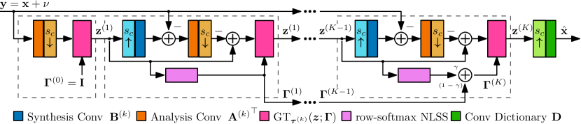
Figure 1: The GroupCDL Architecture. The network begins with no prior of group-sparsity ($\bm{\Gamma}^{(0)}=\bm{I}$). In the second layer, and each subsequent $\Delta K$ layers, the adjacency matrix $\bm{\Gamma}^{(k)}$ is updated by a row-normalized NLSS computation on the latent representation $\bm{z}^{(k)}$. NLSS is computed with dense arithmetic (on image patches) during training, and with sparse arithmetic (on the entire image) during inference.

Approaches in [12, 13, 14] explore the construction of DNNs as unrolled proximal gradient descent machines with proximal-operators that are implemented by a black-box CNN, learned end-to-end. Although these methods contribute to more principled DNN architecture design in image-processing, their use of black-box neural networks, such as UNets [15] and ResNets [16], ultimately side-step the goal of full interpretability. In contrast, our previous work CDLNet [1] introduces a CNN as a direct parameterization of convolutional PGM (4) with an $\ell_{1}$ prior, with layers defined as,

$$\begin{gathered}\bm{z}^{(0)}=\bm{0},\quad\text{for }~{}k=0,1,\dots,K-1,\\ \bm{z}^{(k+1)}=\operatorname{\mathrm{ST}}_{\bm{\tau}^{(k)}}\left(\bm{z}^{(k)}-{\bm{A}^{(k)}}^{T}(\bm{B}^{(k)}\bm{z}^{(k)}-\bm{y})\right),\\ \bm{\tau}^{(k)}=\bm{\tau}^{(k)}_{0}+\hat{\sigma}\bm{\tau}^{(k)}_{1},\quad\hat{\bm{x}}=\bm{D}\bm{z}^{(K)}.\end{gathered}$$ (9)

Parameters $\Theta=\{\bm{D},\,\{{\bm{A}^{T}}^{(k)},\,\bm{B}^{(k)},\,\bm{\tau}_{0}^{(k)},\bm{\tau}^{(k)}_{1}\}_{0=1}^{K-1}\}$ are optimized by back-propagation of a supervised or unsupervised loss function. In this manuscript, we extend the formulation and direct parameterization of CDLNet by introducing a novel implementation of the group-sparsity prior, embodied in the proposed GroupCDL architecture (see Section III). We also show that the noise-adaptive thresholding of CDLNet, derived from BPDN (2), extends to GroupCDL.

Zheng et. al [17] propose a DNN architecture based on a classical dictionary learning formulation of image denoising. However, this network heavily employs black-box models such as UNets [15] and multi-layer perceptrons (MLPs). Our proposed method differentiates itself by using a direct parameterization of variables present in the classical proximal gradient method (4) with a group-sparsity regularizer (6). Furthermore, Zheng et. al’s experimental setup does not match a bulk of the existing image denoising literature (by training on a larger set of images) and their network exists in the ultra-high parameter count regime ($\approx 17$ M), making a fair comparison beyond the scope of this paper.

Directly parameterized dictionary learning networks [1, 3, 2, 18, 4, 5] have gained some popularity in recent years due to their simple design and strong structural similarities to popular ReLU-activation DNNs. This connection was first established in the seminal work of Gregor et. al [19] in the form of the Learned Iterative Shrinkage Thresholding Algorithm (LISTA). Here, we build upon this literature by proposing a novel nonlocal operator (11) for the convolutional dictionary learning formulation of a DNN, derived from a group-sparsity prior (6). We also demonstrate that such a network can compete well with (and sometimes outperform) state-of-the-art methods, without sacrificing interpretability.

Lecouat et. al [2] propose a nonlocal CNN derived from a patch-based dictionary learning algorithm with a group-sparsity prior, dubbed GroupSC. It is well established that the independent processing of image patches and subsequent overlap and averaging (path-processing) is inherently suboptimal to the convolutional model, due to the lack of consensus between pixels in overlapping patch regions [4]. Our method is in-part inspired by GroupSC, but proposes a novel version of the group-sparsity mechanism adapted to the convolutional model and fast application of the network at inference.

II-C Nonlocal Networks

The nonlocal self-similarity prior in image-restoration DNNs is commonly formulated with OW-NLSS to manage its quadratic complexity [6, 2]. The overlap is especially important to ensure that artifacts do not occur on local-window boundaries. Despite such networks often being formulated as CNNs, their window-based inference ultimately diminishes the powerful shift-invariance prior and increases computational cost due to additional processing of overlapping regions (see Section III-B).

To reduce computational burden and correctly account for dependencies between neighboring local windows, we propose a novel sliding-window NLSS, enabled by sparse matrix arithmetic. Recent works have proposed other so-called “sparse attention” mechanisms, however, they have either not been in the context of image restoration [20], not employed a sliding-window [21], or have employed a complicated hashing algorithm to exploit extremely long-range dependencies [22].

III Proposed Method

We consider the problem of image restoration under the AWGN model (1), though, in principle, the methods presented may be adapted to other degradation models with relative ease. Besides being a fundamental building block of many inverse-problem approaches, AWGN is a popular and successful model for camera noise after white-balance and gamma-correction [23].

III-A The GroupCDL Architecture

We propose a neural network architecture as a direct parameterization of PGM (4) on the convolutional BPDN problem with a group-sparsity prior, dubbed GroupCDL. The GroupCDL architecture is equivalent to replacing the CDLNet [1] architecture’s (9) soft-thresholding with group-thresholding w.r.t a row-normalized adjacency matrix $\bm{\Gamma}$, as described in Algorithm 1 and shown in Figure 1. Here, noise-adaptive thresholds are computed using parameters $\bm{\tau}_{0},\,\bm{\tau}_{1}\in\mathbb{R}^{M}_{+}$, ${\bm{A}^{T}}^{(k)},\bm{B}^{(k)}$ are 2D ($C$ to $M$ channel, stride-$s_{c}$) analysis and ($M$ to $C$ channel, stride-$s_{c}$) synthesis convolutions, respectively, and $\bm{D}$ is our 2D ($M$ to $C$ channel, stride-$s_{c}$) synthesis convolutional dictionary. For an input noisy image $\bm{y}\in\mathbb{R}^{NC}$, our latent representation is thus of the form $\bm{z}\in\mathbb{R}^{QM}$, where $Q=N/s_{c}^{2}$.

The adjacency matrix of the group-sparsity prior ($\bm{\Gamma}\in\mathbb{R}^{Q\times Q}_{+}$) encodes similarity between latent subband pixels $\bm{z}[i],\,\bm{z}[j]~{}\forall\,i,\,j$. To manage computational complexity while staying true to the convolutional inductive bias of the network, we form this adjacency using a local sliding-window of size $W\times W$. Motivated by the nonlocal similarity computations of black-box networks [6], we compute the similarity after transforming $\bm{z}[i]$ and $\bm{z}[j]$ along the channel dimension. Specifically, we first compute similarities at the $k$-th layer of the network as,

$$\bm{S}^{(k)}_{ij}=\begin{cases}-\lVert\bm{W}_{\theta}\bm{z}^{(k)}[i]-\bm{W}_{\phi}\bm{z}^{(k)}[j]\rVert_{2}^{2},&\lVert\vec{i}-\vec{j}\rVert_{\infty}\leq W\\ -\infty,&\text{otherwise}\end{cases}$$ (10)

where $\bm{W}_{\theta},\bm{W}_{\phi}\in\mathbb{R}^{M_{h}\times M}$ are learned pixel-wise transforms shared across all layers. That is, similarities $\bm{S}^{(k)}_{ij}$ are only computed for spatial locations $i$ and $j$ within a $W\times W$ window centered on $i$. The similarity matrix is then normalized via a row-wise softmax operation. To reduce computational complexity, we only compute similarity every $\Delta K$ layers. We employ a convex combination of this normalized similarity and the adjacency of the previous layer ($\bm{\Gamma}^{(k-1)}$) with a learned parameter $\gamma\in[0,1]$ (see Alg. 1), to ensure smooth updates. We consider circular boundary conditions when forming nonlocal windows in (10), resulting in a block-circulant with circulant block sparsity pattern for $\bm{S}$ and $\bm{\Gamma}$, as depicted in Figure 2.

Mimicking the use of subband transforms in the similarity computation (10), we introduce two additional subband transforms, $\bm{W}_{\alpha}\in\mathbb{R}^{M\times M_{h}},\bm{W}_{\beta}\in\mathbb{R}_{+}^{M\times M_{h}}$, into the group-thresholding operation,

$$\begin{gathered}\operatorname{\mathrm{GT}}_{\bm{\tau}}(\bm{z};\,\bm{\Gamma})=\bm{z}\circ\left(1-\frac{\bm{\tau}}{\bm{\xi}}\right)_{+},\\ \bm{\xi}=\overline{\bm{W}_{\beta}}\sqrt{(\bm{I}_{M_{h}}\otimes\bm{\Gamma})(\overline{\bm{W}^{T}_{\alpha}}\bm{z})^{2}},\\ \end{gathered}$$ (11)

where $\bm{\xi}\in\mathbb{R}_{+}^{QM}$ contributes to the image-adaptive spatially varying threshold. Here, $\overline{\bm{W}}$ refers to a pixel-wise application of a matrix $\bm{W}$ (see Table I). In contrast to (7), $\bm{W}_{\alpha}$ allows the adjacency-weighted energy of the latent representation to be computed in a compressed subband domain (by setting $M_{h}<<M$). Then, $\bm{W}_{\beta}$ maps this energy back to the uncompressed subband domain ($M$ channels), pixel-wise. In Section IV-E, we empirically show that the use of a compressed subband domain has a positive impact on denoising performance and an even greater impact on reducing inference time.

1 Input: noisy image $\bm{y}$, estimated noise-level $\hat{\sigma}$ ;

2 Parameters: $\Theta=\{\gamma,\,\bm{W}_{\{\theta,\phi,\alpha,\beta\}},\,\bm{D},\,\{{\bm{A}^{T}}^{(k)},\,\bm{B}^{(k)},\,\bm{\tau}^{(k)}_{\{0,1\}}\}_{0=1}^{K-1}\}$ ;

3 Preprocess: $\tilde{\bm{y}}=\bm{y}-\mathrm{mean}(\bm{y})$ ;

4 Initialize: $\bm{z}^{(0)}=\mathbf{0}$, $\bm{\Gamma}^{(0)}=\bm{I}$, $\bm{\tau}^{(k)}=\bm{\tau}^{(k)}_{0}+\hat{\sigma}\bm{\tau}^{(k)}_{1}\,\,\forall\,\,k$ ;

5 for $k=0,1,\dots,K-1$ do

    /​​/Update row-normalized adjacency

6    if $k=1$ then

       $\bm{\Gamma}^{(1)}=\operatorname{\mathbf{softmax}}(\bm{S}^{(1)})$ /​​/Eq. (10)

7      

8   else if $\mathrm{mod}(k+1,\,\Delta K)=0$ then

       $\bm{\Gamma}^{(k)}=\gamma\operatorname{\mathbf{softmax}}(\bm{S}^{(k)})+(1-\gamma)\bm{\Gamma}^{(k-1)}$ /​​/Eq. (10)

9      

10   else

11       $\bm{\Gamma}^{(k)}=\bm{\Gamma}^{(k-1)}$ ;

12      

13   $\bm{r}={\bm{A}^{T}}^{(k)}(\bm{B}^{(k)}\bm{z}^{(k)}-\tilde{\bm{y}})$;

    $\bm{z}^{(k+1)}=\operatorname{\mathrm{GT}}_{\bm{\tau}^{(k)}}\left(\bm{z}^{(k)}-\bm{r};\bm{\Gamma}^{(k)}\right)$ /​​/Eq. (11)

14   

15Output: $\hat{\bm{x}}=\bm{D}\bm{z}^{(K)}+\mathrm{mean}(\bm{y})$ ;

Algorithm 1 Group-sparse Convolutional Dictionary Learning Network (GroupCDL) Forward Pass

III-B Sliding-window vs. Patch based Self-Attention

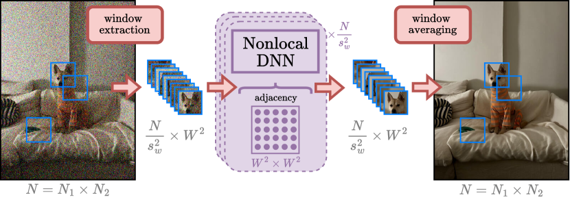
(a) OW-NLSS

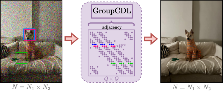
(b) SW-NLSS

Figure 2: (a) In OW-NLSS, the input image is divided into overlapping windows (of size $W\times W$ and with window-stride $s_{w}\times s_{w}$), processed independently via a DNN with dense self-attention. The denoised windows are then placed in their original positions and averaged on their overlaps. (b) In the proposed SW-NLSS, the entire image is processed in a single forward pass, made possible by sparse matrix arithmetic. The adjacency matrix has a block-circulant with circulant blocks (BCCB) sparsity pattern, where the number of non-zeros in each row/column is at most $W^{2}$. The adjacency matrix is computed in the subband domain, with spatial dimension $Q=N/s_{c}^{2}$, where $s_{c}$ is the convolution stride. Hence, the effective image-domain window-size is $s_{c}W\times s_{c}W$.

The SW-NLSS employed by GroupCDL (10) is favorable to the independent OW-NLSS employed by GroupSC [2] and black-box DNNs [6, 24], because it naturally encourages agreement on overlapping regions and centers the nonlocal windows on each pixel. As shown in Figure 2, OW-NLSS additionally incurs computational overhead by processing overlapping pixels multiple times. This burden inherent to OW-NLSS can be expressed in terms of the image dimensions $N=N_{1}\times N_{2}$, window-size $W\times W$, and window-stride $s_{w}\times s_{w}$. We express the burden factor as a ratio of the number of pixels processed by a single OW-NLSS layer over an SW-NLSS layer,

$$\frac{N_{1}/s_{w}\times N_{2}/s_{w}\times W^{2}}{N_{1}\times N_{2}}=\frac{W^{2}}{s_{w}^{2}}.$$ (12)

Common nonlocal window sizes, $45\times 45$, and window-strides, $7\times 7$, such as used by NLRN [6], make this burden factor 41 times the computational complexity of an equivalent SW-NLSS. GroupCDL’s use of strided convolution may add an additional $s_{c}^{2}\times$ computational benefit compared to common NLSS implementations by computing similarities over a reduced spatial dimension $Q=N/s_{c}^{2}$. We further explore the relation between computation time and denoising performance of these two NLSS inference methods in Section IV-D.

III-C Group-Thresholding vs. Black-box Attention

Nonlocal self-similarity is used across domains in DNNs, from transformer architectures [21] to nonlocal image restoration networks [6, 24]. The underlying formula behind these methods is most commonly dot-product attention (DPA), given below,

$$\bm{z}^{(k+1)} =(I_{M_{\mathrm{out}}}\otimes\bm{\Gamma})\overline{\bm{W}_{v}}\bm{z}^{(k)}$$ (13)

$$\bm{\Gamma} =\operatorname{\mathbf{softmax}}(\bm{S}^{(k)})$$ (14)

$$\bm{S}^{(k)}_{ij} =\frac{\bm{z}^{(k)}[j]^{T}\bm{W}_{q}^{T}\bm{W}_{k}\bm{z}^{(k)}[i]}{\sqrt{M_{h}}},$$ (15)

where $\bm{z}^{(k)}\in\mathbb{R}^{NM_{\mathrm{in}}}$, $\bm{W}_{q},\bm{W}_{k},\in\mathbb{R}^{M_{h}\times M_{\mathrm{in}}}$, $\bm{W}_{v}\in\mathbb{R}^{M_{\mathrm{out}}\times M_{\mathrm{in}}}$, and $\bm{z}^{(k+1)}\in\mathbb{R}^{NM_{\mathrm{out}}}$. Learned matrices $\bm{W}_{q},\bm{W}_{k},\bm{W}_{v}$ are understood to transform the input signal $\bm{z}^{(k)}$ to so-called query, key, and value signals.

Both DPA and the proposed GT (11) make use of a normalized adjacency matrix ($\bm{\Gamma}$), computed in an asymmetric feature domain. Both use this adjacency to weight the current spatial features, identically over channels. However, in DPA, the weighting directly results in the layer’s output (via matrix multiplication, see (13)), whereas in GT, this weighting informs a spatially adaptive soft-thresholding.

The proposed GT’s decoupling of adjacency application and output dimension is key in allowing group-thresholding to be computationally efficient, as the adjacency matrix-vector multiplication can be performed in a compressed subband domain. In contrast, DPA operating in a compressed feature domain ($M_{\mathrm{out}}<<M_{\mathrm{in}}$) would harm the capacity of the network’s latent representation. In Section IV-E we show empirical evidence for favoring the negative-norm similarity in GT over the dot-product similarity of DPA.

IV Experimental Results

IV-A Experimental Setup

Architecture: We denote the network detailed in Algorithm 1 as GroupCDL. GroupCDL and CDLNet are trained with noise-adaptive thresholds ($\bm{\tau}^{(k)}=\bm{\tau}^{(k)}_{0}+\hat{\sigma}\bm{\tau}^{(k)}_{1}$) unless specified using the -B suffix, indicating the models are noise-blind ($\bm{\tau}^{(k)}=\bm{\tau}^{(k)}_{0}$). The hyperparameters for these architectures are given in Table II, unless otherwise specified.

TABLE II: Architectures of the GroupCDL models, CDLNet models, and variants presented in the experimental section. We use $C=3$ and $C=1$ for color and grayscale denoising networks, respectively. A filter size of $7\times 7$ is used for all models. Conv-stride $s_{c}=2$, adjacency update period $\Delta K=5$, is used unless otherwise specified.

Name	Task	$K$	$M$	$M_{h}$	$W$
CDLNet(-S,-B)	Gray	30	169	-	-
GroupCDL(-S,-B)	Gray	30	169	64	35
CDLNet(-S,-B)	Color	24	96	-	-
GroupCDL(-S,-B)	Color	24	96	48	35

Dataset and Training: Let $f_{\Theta}$ denote the GroupCDL DNN as a function of parameters $\Theta$. Let $\mathcal{D}=\{(\bm{y},\sigma,\bm{x})\}$ denote a dataset of noisy and ground-truth natural image pairs, with noise-level $\sigma$. Grayscale (and color) GroupCDL models are trained on the (C)BSD432 [25] dataset with the supervised mean squared error (MSE) loss,

$$\underset{\begin{subarray}{c}\bm{W}_{\theta},~{}\bm{W}_{\phi},~{}\bm{W}_{\alpha},\\ \bm{W}_{\beta}\geq 0,~{}\gamma\in[0,1],\\ \bm{D}\in\mathcal{C},~{}\{\bm{\tau}^{(k)}\geq 0\}_{k=0}^{K-1},\\ \{\bm{A}^{(k)}\in\mathcal{C},~{}\bm{B}^{(k)}\in\mathcal{C}\}_{k=0}^{K-1}\end{subarray}}{\mathrm{minimize}}\quad\sum_{\{\bm{y},\sigma,\bm{x}\}\in\mathcal{D}}\lVert f_{\Theta}(\bm{y},\sigma)-\bm{x}\rVert_{2}^{2},$$ (16)

where $\mathcal{C}=\{\bm{D}\,:\,\lVert\bm{D}_{:j}\rVert_{2}^{2}\leq 1~{}\forall\,j\}$. We use the Adam optimizer with default parameters [26], and project the network parameters onto their constraint sets after each gradient step. The dataset is generated online with random crops, rotations, flips, and AWGN of noise-level $\sigma$ sampled uniformly within $\sigma^{\mathrm{train}}$ for each mini-batch element. All models are trained with the same hyperparameters given in [1], however, GroupCDL models are trained for 270k iterations with a batch-size of 32.

Test and validation performance is evaluated on several datasets. The dataset name, along with (arithmetic) average dimensions, are provided to better understand reported inference timings: Set12 (362 $\times$ 362), CBSD68 [25] (481 $\times$ 321), Urban100 [27] (1030 $\times$ 751), and NikoSet10 (1038 $\times$ 779).

Training Initialization: CDLNet models are initialized as ISTA with $\bm{\tau}_{0}=10^{-2},~{}\bm{\tau}_{1}=0$, and a base dictionary $\bm{D}$ that has been spectrally normalized. Details are given in [1]. GroupCDL models are initialized with a trained CDLNet model. Pixel-wise transforms $\bm{W}_{\{\theta,\phi,\alpha\}}$ are initialized with the same weights drawn from a Glorot Uniform distribution centered at zero [28], and $\bm{W}_{\beta}$ is drawn from a similar Glorot Uniform distribution, tailored to the positive orthant. We initialize parameter $\gamma=0.8$.

Group-Thresholding Training vs. Inference: A GroupCDL model, with nonlocal window-size $W$ and conv-stride $s_{c}$, is trained using image crops of dimension $s_{c}W\times s_{c}W$ such that a single nonlocal window is used during training. Dense arithmetic is used in construction and application of the normalized adjacency matrix $\bm{\Gamma}^{(k)}$ throughout training.

On inference of a noisy image $\bm{y}\in\mathbb{R}^{NC}$, with latent representation $\bm{z}\in\mathbb{R}^{QM}$ ($Q=N/s_{c}^{2}$), the adjacency matrix $\bm{\Gamma}~{}\in~{}\mathbb{R}_{+}^{Q\times Q}$ is constructed with a block circulant with circulant blocks (BCCB) sparsity pattern and sparse matrix arithmetic is used. The adjacency matrix requires an allocation of $Q\times W^{2}\times\text{{sizeof(float)}}$ bytes. For a high resolution image of size $1024\times 1024$ (such as images in the Urban100 dataset [27]) and a conv-stride of $2$, this results in roughly $2.6$ GB of memory required to store $\bm{\Gamma}^{(k)}$ and $\bm{\Gamma}^{(k-1)}$, which is by and large the memory consumption of inference.

Hardware: All models were trained on a single core Intel Xeon CPU with 2.90 GHz clock and a single NVIDIA A100 GPU. CDLNet pre-training takes roughly 6 hours, and GroupCDL training takes approximately an additional 36 hours. Note that training and inference can take place on GPUs with as low as 16 GB of memory. For code-base compatibility reasons, all inference timings in Tables III, IV were determined by running models (provided by the authors of the respective papers), and our trained GroupCDL/CDLNet models, on a single core Intel Xeon CPU with 2.90 GHz clock and a NVIDIA Quadro RTX-8000 GPU.

IV-B Single Noise-Level Performance

In this section, we demonstrate the fast inference speed and competitive denoising performance of the proposed GroupCDL. All models are trained on a single noise-level and tested at the same noise-level ($\sigma^{\mathrm{train}}=\sigma^{\mathrm{test}}$). We compare GroupCDL to its fully convolutional counterpart (CDLNet), the non-learned nonlocal method BM3D [29, 30], popular local and nonlocal black-box CNNs [31, 32, 6], and a patch-processing dictionary learning based nonlocal DNN (GroupSC) [2].

TABLE III: Grayscale denoising performance (PSNR (dB)/ $100\times$SSIM) and GPU inference runtimes. All learned methods are trained on BSD432 [25] with an MSE loss function ($\sigma=\sigma^{\mathrm{train}}=\sigma^{\mathrm{test}}$). Learned parameter counts are displayed below the method names.

Dataset	Noise $\sigma$	BM3D [29]	DnCNN [31]	CDLNet [1]	GroupSC [2]	GCDN [32]	NLRN [6]	GroupCDL-S
		-	556k	507k	68k	6M	340k	550k
Set12	15	32.37/89.52	32.86/90.31	32.87/90.43	32.85/90.63	33.14/90.72	33.16/90.70	33.05/90.73
	25	29.97/85.04	30.44/86.22	30.52/86.55	30.44/86.42	30.78/86.87	30.80/86.89	30.75/86.93
	50	26.72/76.76	27.18/78.29	27.42/79.41	27.14/77.97	27.60/79.57	27.64/79.80	27.63/80.04
time (s)		0.010	0.119	0.019	22.07	404.8	25.62	0.68
BDS68 [25]	15	31.07/87.17	31.73/89.07	31.74/89.18	31.70/89.63	31.83/89.33	31.88/89.32	31.82/89.41
	25	28.57/80.13	29.23/82.78	29.26/83.06	29.20/83.36	29.35/83.32	29.41/83.31	29.38/83.51
	50	25.62/68.64	26.23/71.89	26.35/72.69	26.17/71.83	26.38/73.89	26.47/72.98	26.47/73.32
time (s)		0.011	0.039	0.022	23.63	539.7	26.66	0.65
Urban100 [27]	15	32.35/92.20	32.68/92.55	32.59/92.85	32.72/93.08	33.47/93.58	33.42/93.48	33.07/93.40
	25	29.70/87.77	29.92/87.97	30.03/89.00	30.05/89.12	30.95/90.20	30.88/90.03	30.61/90.03
	50	25.95/77.91	26.28/78.74	26.66/81.11	26.43/80.02	27.41/81.60	27.40/82.44	27.29/83.05
time (s)		0.030	0.096	0.090	93.33	1580	135.8	3.56

TABLE IV: Color Denoising performance, PSNR (dB), and GPU inference runtimes on CBSD68 [25] . All learned methods are trained on CBSD432 [25] ($\sigma=\sigma^{\mathrm{train}}=\sigma^{\mathrm{test}}$).

Model	Params	time (s)	Noise-level ($\sigma$)
			10	15	25	30	50
BM3D [29]	-	0.019	34.56	33.49	30.68	28.05	27.36
DnCNN [31]	668k	0.054	36.31	33.99	31.31	-	28.01
CDLNet	694k	0.009	36.31	34.04	31.39	30.52	28.18
GroupSC [2]	119k	40.81	36.40	34.11	31.44	30.58	28.05
RNAN [24]	8.96M	1.92	36.60	-	-	30.73	28.35
GroupCDL-S	698k	0.39	36.43	34.19	31.58	30.70	28.37

(a) Noisy
20.38/45.63

(b) CDLNet [1]
29.49/86.56

(c) GroupSC [2]
29.43/86.35

(d) NLRN [6]
29.97/87.19

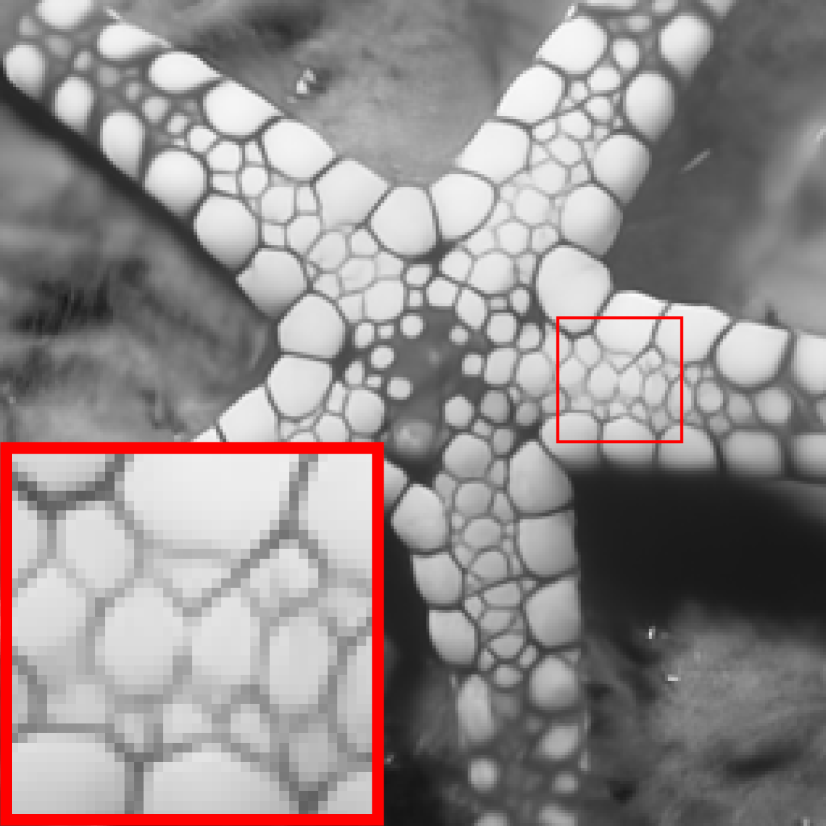
(e) GCDN [32]
29.93/87.22

(f) GroupCDL
29.87/87.18

Figure 3: Visual comparison for grayscale denoising models ($\sigma^{\mathrm{test}}=\sigma^{\mathrm{train}}=25$) on the starfish test image. PSNR (dB)/$100\times$SSIM reported for each image.

Table III shows the grayscale denoising performance and inference speed of the aforementioned models across several common datasets. We include a learned parameter count as a crude measure of expressivity of the model. The group-sparsity prior of GroupCDL significantly increases denoising performance compared to the unstructured sparsity prior of CDLNet, though at a detriment to inference speed. We observe that GroupCDL has denoising performance superior to other dictionary learning based networks using group sparsity prior (GroupSC) and competitive performance with state-of-the-art black-box methods (GCDN, NLRN). Most notably, GroupCDL has the fastest inference runtime among nonlocal methods, with at least an order of magnitude difference. These timing differences between GroupCDL and NLRN (or GroupSC) correspond well with the analysis in Section III-B regarding the use of sliding-window sparse nonlocal processing vs. overlapping-window nonlocal processing.

Table IV shows the color image denoising performance and inference speed of the aforementioned classical benchmark [29, 30], local DNN [31], nonlocal patch-processing DNN [2], and black-box nonlocal DNN [24] against the proposed GroupCDL. We observe that GroupCDL outperforms the interpretable patch-processing dictionary learning DNN (GroupSC) and CNNs (DnNN, CDLNet). GroupCDL performs competitively to the black-box nonlocal DNN (RNAN [24]) at a faction of the learned parameter count and inference time.

(a) Noisy
18.01/24.57

(b) CDLNet [1]
28.63/79.37

(c) GroupSC [2]
28.68/79.65

(d) RNAN [24]
28.78/80.22

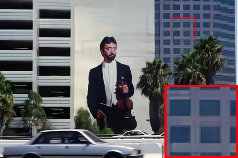
(e) GroupCDL
28.80/80.26

(f) Noisy
18.12/15.75

(g) CDLNet [1]
30.53/75.43

(h) GroupSC [2]
30.39/75.20

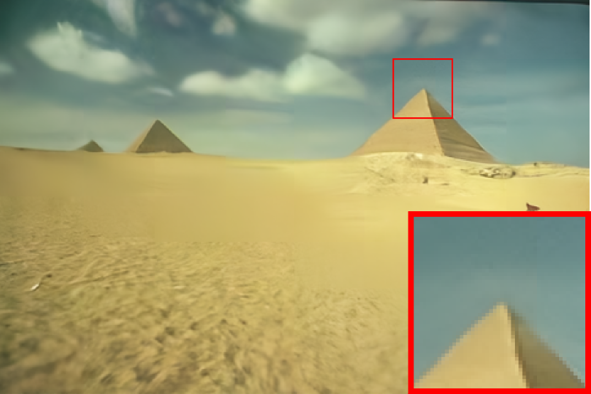
(i) RNAN [24]
30.54/75.27

(j) GroupCDL
30.69/76.22

(k) Noisy
20.52/34.79

(l) CDLNet [1]
31.10/87.70

(m) GroupSC [2]
31.06/87.44

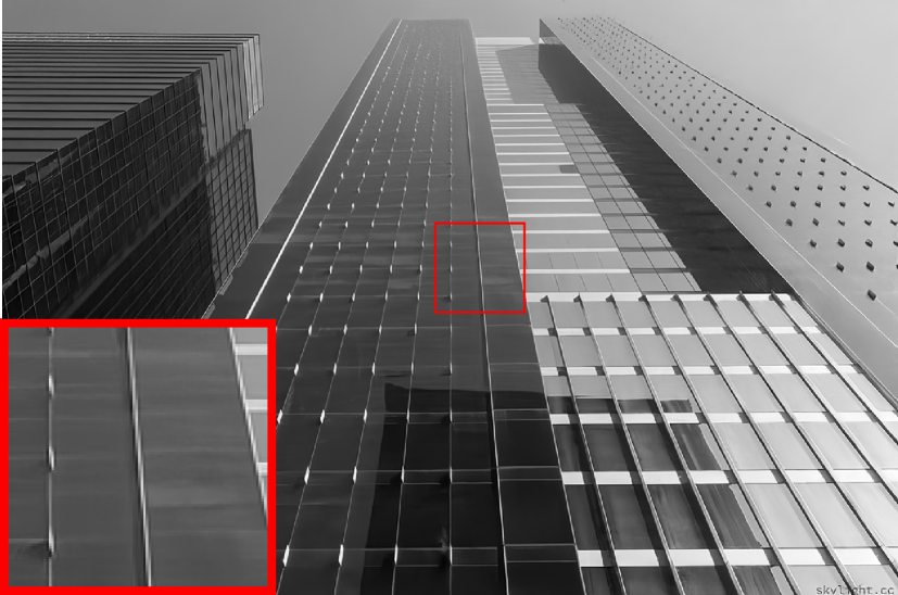
(n) NLRN [6]
32.20/89.46

(o) GroupCDL
31.96/89.55

Figure 4: Visual comparison of deep denoisers. Top and middle rows: color denoisers for $\sigma^{\mathrm{train}}=\sigma^{\mathrm{test}}=50$. Bottom row: grayscale denoisers $\sigma^{\mathrm{train}}=\sigma^{\mathrm{test}}=25$. PSNR/$100\times$SSIM shown in respective captions.

Figures 3 and 4 highlight the qualitative differences between the previously mentioned methods. We observe that the group-sparsity prior of GroupCDL is instrumental in suppressing unwanted denoising artifacts (present in CDLNet’s results), especially in constant image regions where edges are otherwise hallucinated (see Figure 4 (g) vs (j)). Note that GroupSC produces low spatial-frequency artifacts throughout the image, likely introduced by independent processing of image patches (see Figure 4 (c,h,m)). Further, GroupCDL’s results appear qualitatively indistinguishable to those of state-of-the-art black-box models, at a fraction of the inference time.

IV-C Noise-Level Generalization

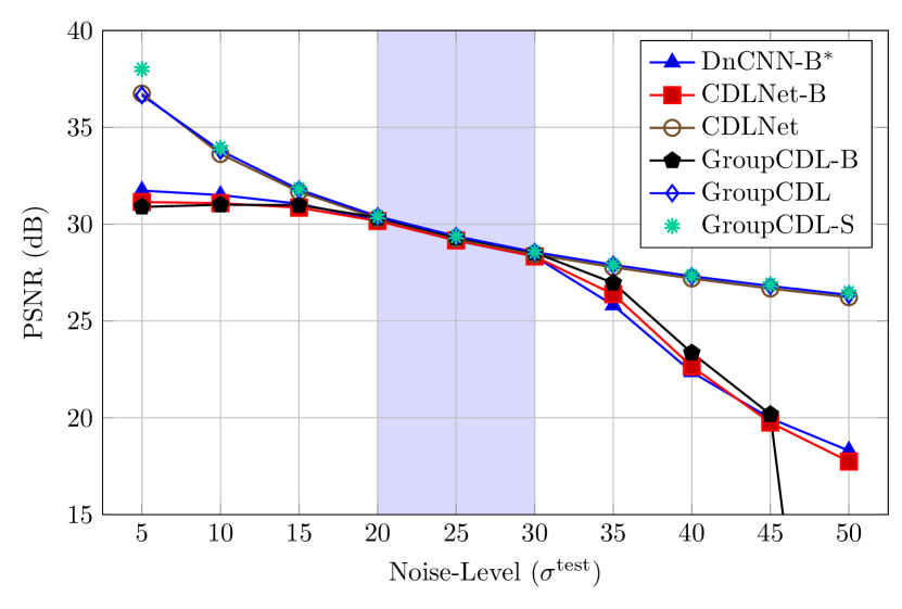
Figure 5: Noise-level generalization of different grayscale denoising networks tested on BSD68 [25]. GroupCDL-S is trained at $\sigma^{\mathrm{test}}$ for each point on the graph. All other networks are trained on $\sigma^{\mathrm{train}}=[20,30]$.

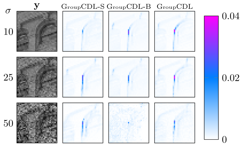
Figure 6: Visualization of normalized adjacency $\bm{\Gamma}^{(K)}_{i:}$ for input nonlocal window $\bm{y}$ at noise-levels $\sigma=10,25,50$. Columns GroupCDL-S, GroupCDL-B, and GroupCDL visualize the adjacency of models trained under conditions of $\sigma^{\mathrm{train}}=\sigma$, $\sigma^{\mathrm{train}}\in[20,30]$ without noise-adaptive thresholds, and $\sigma^{\mathrm{train}}\in[20,30]$ with noise-adaptive thresholds, respectively. Catastrophic failure of GroupCDL-B model is observed for $\sigma>\sigma^{\mathrm{train}}$. The same noise-realization is used across models and noise-levels (with appropriate scaling).

In this section, we look at the denoising performance of trained denoising DNNs on inference of input images with noise-levels ($\sigma^{\mathrm{test}}$) outside their training noise-level range ($\sigma^{\mathrm{train}}$). Figure 5 shows the performance of grayscale image denoisers, trained over the range $\sigma^{\mathrm{train}}=[20,30]$. The figure shows, as also noted in [33, 1, 3], black-box DNNs (such as DnCNN [31]) and dictionary learning DNNs without noise-adaptive thresholds exhibit a catastrophic failure on inference above their training noise-level range. A less striking but analogous failure is seen on inference below the training noise-level, where a mere plateau in performance is obtained as the denoising problem becomes easier.

In addition to the observations noted in [1], Figure 5 shows that the proposed novel group-thresholding scheme (11) is able to obtain near-perfect noise-level generalization (w.r.t GroupCDL-S performance). This serves as empirical evidence for the interpretation of the unrolled network as performing some approximate/accelerated group-sparse BPDN, as the noise-adaptive thresholds ($\bm{\tau}=\bm{\tau}_{0}+\hat{\sigma}\bm{\tau}_{1}$) appear to correspond very well to their classical counter-parts from which they are derived.

We further investigate the behavior of the proposed group-thresholding across noise-levels in Figure 6. The figure shows a single input nonlocal window $\bm{y}$ across noise-levels $\sigma$ and the computed adjacency values of the three types of GroupCDL models (GroupCDL-S, GroupCDL-B, GroupCDL).

In agreement with the catastrophic failure of the noise-level blind GroupCDL-B model of Figure 5, the adjacency visualizations of GroupCDL-B in Figure 6 show a catastrophic failure in the similarity computations of the network above $\sigma^{\mathrm{train}}$, as no structure is found. We observe a similar pattern in the GroupCDL models (with noise-adaptive thresholds) to the visualizations of GroupCDL-S, however, the single noise-level models seem to have more variation in their computed similarities across noise-levels. This could suggest room for improvement in GroupCDL by parametrizing the similarity computations of (7) and (10) to also be noise-adaptive. However, this subtle dissimilarity may also be due to the fact that each row-element for the GroupCDL-S column in Figure 6 is from a different trained model with different weights (i.e. with similarities computed in different domains), whereas the visualizations from the GroupCDL column are all from the same model.

IV-D Sliding vs. Overlapping Window Nonlocal Processing

From Figure 2, it is clear that the OW-NLSS strategy (used by NLRN [6] and GroupSC [2]) is able to achieve a denoising to speed trade-off by reducing the amount of overlap between windows, i.e. increasing window-stride ($s_{w}$). SW-NLSS can also achieve a similar performance-speed trade-off by instead reducing the nonlocal window-size ($W$) during inference.

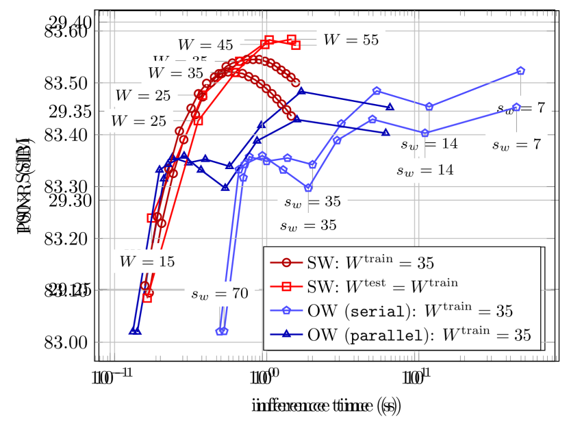
Figure 7: Inference-time vs. denoising-performance trade-off for GroupCDL. Circle, pentagon, and triangle markers are generated by the same trained GroupCDL model ($W^{\mathrm{train}}=35$) under different inference strategies (SW-NLSS w/ window-size $W$, OW-NLSS w/ window-stride $s_{w}$). The square markers are each generated by a GroupCDL with a different training window-size $W^{\mathrm{train}}$. Performance (a) PSNR, (b) $100\times$SSIM, is evaluated on BSD68 [25] with $\sigma^{\mathrm{train}}=\sigma^{\mathrm{test}}=25$. OW-NLSS (serial,parallel) curves are generated via processing independent overlapping windows either sequentially or all at once, respectively. The same noise-realization for the dataset was used across all evaluations plotted. Note that $W$ corresponds between SW curve markers vertically (the same inference time), and $s_{w}$ corresponds between OW curve markers horizontally (the same PSNR/SSIM).

(a) Noisy

(b) $s_{w}=70$, 29.59 / 82.83 / 0.09

(c) $s_{w}=35$, 29.72 / 83.29 / 0.33

(d) $s_{w}=32$, 29.72 / 83.45 / 0.40

(e) Ground Truth

(f) $W=15$, 29.57 / 82.92 / 0.08

(g) $W=25$, 29.79 / 83.69 / 0.16

(h) $W=35$, 29.83 / 83.75 / 0.29

Figure 8: Comparison of inference-speed/denoising trade-off between OW-NLSS (b-d) and SW-NLSS (f-h) processing by a color GroupCDL model ($\sigma^{\mathrm{train}}=\sigma^{\mathrm{test}}=50$, $W^{\mathrm{train}}=35$). PSNR (dB) / $100\times$SSIM / GPU inference-time (s) shown in respective captions. Zoomed-in regions highlight blocking artifacts exist across shown OW-NLSS window-strides ($s_{w}$), whereas SW-NLSS processing exhibits no blocking artifacts across inference window-sizes ($W$). Yellow arrows (b-d) point to specific blocking artifact boundaries of OW-NLSS. Orange arrows (f) point to edge/texture hallucination artifacts of SW-NLSS with a small windowsize. The inclusion of (d) ($s_{w}=32$), demonstrates that blocking artifacts are not merly a result of the effective spatial windowsize ($s_{c}W=70$) being divisible by the overlapping window-stride. The same noise-realization is used across all methods (b-d, f-h).

Figure 7 plots the denoising performance vs. inference time trade-off attainable by GroupCDL under the SW-NLSS strategy and the OW-NLSS strategy. The SW: $W^{\mathrm{train}}=35$, and OW curves show a single GroupCDL model (trained with a nonlocal window-size $W^{\mathrm{train}}=35$) under SW-NLSS inference with varying nonlocal window-size $W^{\mathrm{test}}$, and OW-NLSS inference with varying window-stride $s_{w}$, respectively. Each point in the SW: $W^{\mathrm{train}}=W^{\mathrm{test}}$ curve shows the performance of a GroupCDL model trained with a different non-local window-size and performing SW-NLSS inference with their respective training window-size.

First, we observe that SW-NLSS consistently out-performs OW-NLSS across the PSNR-speed and SSIM-speed trade-offs – in both parallel and serial window processing forms of OW-NLSS. This agrees well with the burden-factor analysis in Section III-B. The curves further highlight that competitive denoising performance in OW-NLSS inference is predicated on using a small window-stride, in order to compensate for the neglect of dependencies between overlapping window regions by window-averaging. Second, we observe that increasing the training window-size $W^{\mathrm{train}}$ has diminishing returns on denoising performance. This is consistent with the intuition that non-local similarities of natural images are generally located close to the pixel of interest. Lastly, we observe that the OW-NLSS curves of Figure 7 are not monotonically increasing with smaller window-stride, and in-fact have significant drops in the SSIM curves (Fig. 7 (b), blue triangle and pentagon curves). The source of this behavior is windowing artifacts, highlighted visually in Figure 8. These visualizations show that the denoising-speed trade-off exhibited by OW-NLSS processing comes with the penalty of unnatural artifacts in the form of grid-lines corresponding to the spatial pattern of window overlaps. In contrast, the proposed SW-NLSS does not exhibit windowing artifacts. Instead, as the window-size decreases, SW-NLSS processing transitions to fully convolutional CDLNet processing, and artifacts associated with FCNNs (such as hallucinated edges) are observed.

IV-E Ablation Studies

In this section we examine the denoising and inference time performance of the GroupCDL model under different hyperparameters associated with the proposed group-thresholding operation (11), (10). Table V shows the effect of the update-period parameter ($\Delta K$), which determines how often we update the adjacency $\bm{\Gamma}^{(k)}$ in the network (every $\Delta K$ layers, see Alg. 1). We observe that decreasing the update frequency increases denoising performance, with diminishing returns, at cost to the inference speed of the network.

TABLE V: Effect of update frequency ($\Delta K$). Grayscale denoising performance averaged over the NikoSet10 dataset ($\sigma^{\mathrm{train}}=\sigma^{\mathrm{test}}=25$).

$\Delta K$	PSNR/$100\times$SSIM	time (s)
2	30.22/86.88	4.01
3	30.22/86.87	4.72
5	30.21/86.87	3.47
10	30.21/86.87	3.24
15	30.19/86.79	3.18

TABLE VI: Effect of NLSS feature compression. Grayscale denoising performance averaged over the NikoSet10 dataset ($\sigma^{\mathrm{train}}=\sigma^{\mathrm{test}}=25$).

feature-compression	$M_{h}$	sim_fun	PSNR/$100\times$SSIM	time (s)
none	n/a	-distance	30.19/86.79	8.64
$\bm{W}_{\{\theta,\phi\}}$	64	-distance	30.21/86.86	8.13
$\bm{W}_{\{\theta,\phi,\alpha,\beta\}}$	169	-distance	30.21/86.89	8.89
$\bm{W}_{\{\theta,\phi,\alpha,\beta\}}$	64	-distance	30.21/86.87	3.47
$\bm{W}_{\{\theta,\phi,\alpha,\beta\}}$	32	-distance	30.20/86.84	2.00
$\bm{W}_{\{\theta,\phi,\alpha,\beta\}}$	64	dot	30.11/86.55	3.43

Table VI shows the effect of employing learned pixel-wise transforms in the similarity computation (10) ($\bm{W}_{\theta}$, $\bm{W}_{\phi}$) and group-thresholding (11) ($\bm{W}_{\alpha}$, $\bm{W}_{\beta}$). The table also shows the effect of employing channel reduction in these transforms ($M_{h}<<M=169$) and a comparison of using the negative distance similarity (as presented in (10)) or, as more commonly used in black-box nonlocal and transformer DNNs, the dot-product similarity (15). From these experiments, we observe that the use of pixel-wise transforms increases denoising performance. Most importantly, we observe only a marginal decrease in performance for setting the latent similarity channel dimension less than the latent subband dimension $M_{h}<M$. This marginal decrease is met by a massive reduction in GPU inference time, which is predicted well by the channel reduction ration $M/M_{h}=169/64\approx 8.89/3.47$. This demonstrates one of the advantages of the proposed group-thresholding operation over black-box dot-product attention, in that the latent similarity channel dimension $M_{h}$ is decoupled from the layer’s output channel dimension and can be tuned to achieve a better trade-off between speed and performance.

V Discussion and Conclusion

GroupCDL adapts the classical, patch-processing based, group-sparsity prior to convolutional sparse coding (CSC) and applies it to the direct-parametrization unrolling frame-work of CDLNet [1]. In contrast to the group-sparsity prior of Lecouat et. al’s patch-based dictionary learning network (GroupSC) [2], which employ’s overlapping window processing, we formulate our group-sparsity prior on convolutional sparse codes, and in doing so naturally arrive at a sliding-window nonlocal self-similarity consistent with the CSC model. As discussed in Section III-B and empirically validated in Section IV-D, the proposed SW-NLSS enjoys an improved denoising performance over OW-NLSS by properly accounting for correlations between neighboring image regions and centering similarity computations on each latent pixel of interest. The sparse array arithmetic employed at inference time, enables orders of magnitude speed-up for the proposed design compared to state-of-the-art competitor networks (Section IV-B).

Notably, GroupCDL’s performance comes without the use of common deep-learning operations, such as batch-normalization [34] or residual learning [31], and instead relies on the tools of classical signal processing and optimization such as basis-pursuit denoising and proximal operators.

The fast inference of GroupCDL is aided by a novel decoupling of the latent subband dimension ($M$) from the hidden adjacency/similarity dimension ($M_{h}$) (see Equation (11)). This allows the computational bottleneck of sparse-matrix dense-vector multiplication to be tuned without harming the capacity of the latent representation (Table VI) – something which is not achievable in the dot-product attention employed by black-box nonlocal and transformer networks (Section III-B).

Similar to CDLNet [1], GroupCDL is formulated as a direct parameterization of the proximal gradient method (4). We show that this derivation allows for near perfect generalization outside of its training noise-level range (Fig. 5), simply by parametrizing its thresholds as an affine function of the input noise-level, as suggested by the classical BPDN formulation (2) and the universal thresholding theorem [8, 1]. In contrast, black-box networks [31] are shown to fail catastrophically above the noise-level range and simply plateau in performance when the noise-level decreases (i.e. the problem becomes easier). In GroupCDL, generalization is additionally observed in its adjacency matrix (Fig. 6).

In future work, we aim to adapt GroupCDL to other imaging modalities. We believe GroupCDL’s speed, performance, interpretability, and robustness are well suited to tackle large signal reconstruction problems with nonlocal image-domain artifacts, such compressed sensing magnetic resonance imaging. The unsupervised learning and demosaicing work of CDLNet [1] may be adapted for GroupCDL to this end.

References

- [1] N. Janjušević, A. Khalilian-Gourtani, and Y. Wang, “CDLNet: Noise-adaptive convolutional dictionary learning network for blind denoising and demosaicing,” IEEE Open Journal of Signal Processing, vol. 3, pp. 196–211, 2022.
- [2] B. Lecouat, J. Ponce, and J. Mairal, “Fully trainable and interpretable non-local sparse models for image restoration,” in European Conference on Computer Vision (ECCV), 2020.
- [3] N. Janjušević, A. Khalilian-Gourtani, and Y. Wang, “Gabor is enough: Interpretable deep denoising with a gabor synthesis dictionary prior,” in 2022 IEEE 14th Image, Video, and Multidimensional Signal Processing Workshop (IVMSP), 2022, pp. 1–5.
- [4] D. Simon and M. Elad, “Rethinking the CSC model for natural images,” in Advances in Neural Information Processing Systems, 2019, pp. 2274–2284.
- [5] M. Scetbon, M. Elad, and P. Milanfar, “Deep k-svd denoising,” IEEE Transactions on Image Processing, vol. 30, pp. 5944–5955, 2019.
- [6] D. Liu, B. Wen, Y. Fan, C. C. Loy, and T. S. Huang, “Non-local recurrent network for image restoration,” in Advances in Neural Information Processing Systems, 2018, pp. 1680–1689.
- [7] J. Bezanson, A. Edelman, S. Karpinski, and V. B. Shah, “Julia: A fresh approach to numerical computing,” SIAM Review, vol. 59, no. 1, pp. 65–98, 2017. [Online]. Available: https://doi.org/10.1137/141000671
- [8] S. Mallat, A Wavelet Tour of Signal Processing: The Sparse Way. Elsevier Science, 2008.
- [9] A. Beck and M. Teboulle, “A fast iterative shrinkage-thresholding algorithm for linear inverse problems,” SIAM Journal on Imaging Sciences, vol. 2, pp. 183–202, 01 2009.
- [10] J. Mairal, F. Bach, J. Ponce, G. Sapiro, and A. Zisserman, “Non-local sparse models for image restoration,” in Proceedings of 12th IEEE International Conference on Computer Vision (ICCV), 2009, pp. 2272–2279.
- [11] J. Mairal, F. Bach, J. Ponce, and G. Sapiro, “Online dictionary learning for sparse coding,” in Proceedings of the 26th International Conference on Machine Learning (ICML), 2009, pp. 689–696.
- [12] G. Ongie, A. Jalal, C. A. Metzler, R. G. Baraniuk, A. G. Dimakis, and R. Willett, “Deep learning techniques for inverse problems in imaging,” IEEE Journal on Selected Areas in Information Theory, vol. 1, no. 1, pp. 39–56, 2020.
- [13] D. Gilton, G. Ongie, and R. Willett, “Neumann networks for linear inverse problems in imaging,” IEEE Transactions on Computational Imaging, vol. 6, pp. 328–343, 2019.
- [14] ——, “Deep equilibrium architectures for inverse problems in imaging,” IEEE Transactions on Computational Imaging, vol. 7, pp. 1123–1133, 2021.
- [15] O. Ronneberger, P. Fischer, and T. Brox, “U-Net: Convolutional networks for biomedical image segmentation,” Medical Image Computing and Computer-Assisted Intervention, p. 234–241, 2015.
- [16] K. He, X. Zhang, S. Ren, and J. Sun, “Deep residual learning for image recognition,” in Proceedings of the IEEE conference on computer vision and pattern recognition, 2016, pp. 770–778.
- [17] H. Zheng, H. Yong, and L. Zhang, “Deep convolutional dictionary learning for image denoising,” in Proceedings of the IEEE/CVF Conference on Computer Vision and Pattern Recognition (CVPR), June 2021, pp. 630–641.
- [18] H. Sreter and R. Giryes, “Learned convolutional sparse coding,” in Proceedings of IEEE International Conference on Acoustics, Speech and Signal Processing (ICASSP), 2018, pp. 2191–2195.
- [19] K. Gregor and Y. LeCun, “Learning fast approximations of sparse coding,” in Proceedings of the 27th International Conference on Machine Learning (ICML), 2010, pp. 399–406.
- [20] R. Child, S. Gray, A. Radford, and I. Sutskever, “Generating long sequences with sparse transformers,” URL https://openai.com/blog/sparse-transformers, 2019.
- [21] T. Dao, D. Y. Fu, S. Ermon, A. Rudra, and C. Ré, “FlashAttention: Fast and memory-efficient exact attention with IO-awareness,” in Advances in Neural Information Processing Systems, 2022.
- [22] Y. Mei, Y. Fan, and Y. Zhou, “Image super-resolution with non-local sparse attention,” in Proceedings of the IEEE/CVF Conference on Computer Vision and Pattern Recognition (CVPR), June 2021, pp. 3517–3526.
- [23] D. Khashabi, S. Nowozin, J. Jancsary, and A. W. Fitzgibbon, “Joint demosaicing and denoising via learned nonparametric random fields,” IEEE Transactions on Image Processing, vol. 23, pp. 4968–4981, 2014.
- [24] Y. Zhang, K. Li, B. Zhong, and Y. Fu, “Residual non-local attention networks for image restoration,” in International Conference on Learning Representations, 2019.
- [25] D. Martin, C. Fowlkes, D. Tal, and J. Malik, “A database of human segmented natural images and its application to evaluating segmentation algorithms and measuring ecological statistics,” in Proceedings of 8th IEEE International Conference on Computer Vision (ICCV), vol. 2, 2001, pp. 416–423.
- [26] D. P. Kingma and J. Ba, “Adam: A method for stochastic optimization,” in International Conference on Learning Representations (ICLR), 2015.
- [27] J.-B. Huang, A. Singh, and N. Ahuja, “Single image super-resolution from transformed self-exemplars,” in Proceedings of the IEEE Conference on Computer Vision and Pattern Recognition (CVPR), June 2015.
- [28] X. Glorot and Y. Bengio, “Understanding the difficulty of training deep feedforward neural networks,” in Proceedings of the Thirteenth International Conference on Artificial Intelligence and Statistics, ser. Proceedings of Machine Learning Research, Y. W. Teh and M. Titterington, Eds., vol. 9. Chia Laguna Resort, Sardinia, Italy: PMLR, 13–15 May 2010, pp. 249–256. [Online]. Available: https://proceedings.mlr.press/v9/glorot10a.html
- [29] K. Dabov, A. Foi, V. Katkovnik, and K. Egiazarian, “Image denoising by sparse 3-D transform-domain collaborative filtering,” IEEE Transactions on Image Processing, vol. 16, no. 8, pp. 2080–2095, 2007.
- [30] D. Honzátko and M. Kruliš, “Accelerating block-matching and 3d filtering method for image denoising on gpus,” 11 2017.
- [31] K. Zhang, W. Zuo, Y. Chen, D. Meng, and L. Zhang, “Beyond a gaussian denoiser: Residual learning of deep CNN for image denoising,” IEEE Transactions on Image Processing, vol. 26, no. 7, p. 3142–3155, 2017.
- [32] D. Valsesia, G. Fracastoro, and E. Magli, “Deep graph-convolutional image denoising,” IEEE Transactions on Image Processing, vol. 29, pp. 8226–8237, 2020.
- [33] S. Mohan, Z. Kadkhodaie, E. P. Simoncelli, and C. Fernandez-Granda, “Robust and interpretable blind image denoising via bias-free convolutional neural networks,” in International Conference on Learning Representations (ICLR), 2020.
- [34] S. Ioffe and C. Szegedy, “Batch normalization: Accelerating deep network training by reducing internal covariate shift,” in International conference on machine learning. PMLR, 2015, pp. 448–456.