Excitations of quantum Ising chain CoNb2O6 in low transverse field: quantitative description of bound states stabilized by off-diagonal exchange and applied field

Abstract

We present experimental and theoretical evidence of novel bound state formation in the low transverse field ordered phase of the quasi-one-dimensional Ising-like material CoNb2O6. High resolution single crystal inelastic neutron scattering measurements observe that small transverse fields lead to a breakup of the spectrum into three parts, each evolving very differently upon increasing field. This can be naturally understood starting from the excitations of the ordered phase of the transverse field Ising model, domain wall quasiparticles (solitons). Here, the transverse field and a staggered off-diagonal exchange create one-soliton hopping terms with opposite signs. We show that this leads to a rich spectrum and a special field, when the strengths of the off-diagonal exchange and transverse field match, at which solitons become localized; the highest field investigated is very close to this special regime. We solve this case analytically and find three two-soliton continua, along with three novel bound states. Perturbing away from this novel localized limit, we find very good qualitative agreement with the experimental data. We also present calculations using exact diagonalization of a recently refined Hamiltonian model for CoNb2O6 and using diagonalization of the two-soliton subspace, both of which provide a quantitative agreement with the observed spectrum. The theoretical models qualitatively and quantitatively capture a variety of non-trivial features in the observed spectrum, providing insight into the underlying physics of bound state formation.

I Introduction

The transverse field Ising chain (TFIC) is an important model in condensed matter physics because it displays the key paradigms of both a continuous quantum phase transition from an ordered phase to a quantum paramagnetic phase as a function of field, as well as, in the ordered phase, of fractionalization of local spin flips into pairs of domain wall quasiparticles (solitons) [1]. The pure TFIC model can be mapped to non-interacting fermions [2, 3], which in the ordered phase represent these solitons. However, a variety of different additional subleading terms in the spin Hamiltonian, such as a longitudinal field [4] or an XY exchange [5] can stabilize two-soliton bound states. Here we explore a regime where novel bound states can be stabilized by the interplay of applied transverse field and off-diagonal exchange.

The material CoNb2O6 has been seen as a realization of TFIC physics for over a decade [5, 6, 7, 8, 9]. Among the key experimental observations is the qualitative change in the nature of quasiparticles from domain walls in the ordered phase to coherently propagating spin flips in the high-field paramagnetic phase. Moreover, a fine structure of bound states was observed just below the critical transverse field, consistent with predictions for a universal E8 spectrum expected in the presence of a perturbing longitudinal field, which in this case arises from mean-field effects of the three dimensional magnetic order [5, 9]. The crystal structure is orthorhombic (space group $Pbcn$), with Co^2+ ions with effective spin-$\frac{1}{2}$ arranged in zigzag chains running along the $c$-axis, with dominant nearest-neighbour ferromagnetic Ising exchange (see Fig. 1A). At the lowest temperatures, small three-dimensional interactions between chains stabilize a ground state with ferromagnetic ordering along the zigzag chains and with an antiferromagnetic pattern between chains [10, 11, 12, 13, 14]. While the dominant magnetic physics in CoNb2O6 can be captured by a TFIC Hamiltonian, additional terms in the Hamiltonian beyond the dominant Ising exchange are needed to explain various features of the spectrum [5, 15]. In particular, a staggered off-diagonal exchange term was recently proposed on symmetry grounds and shown to reproduce well the zero-field spectrum using density matrix renormalization group numerics [15].

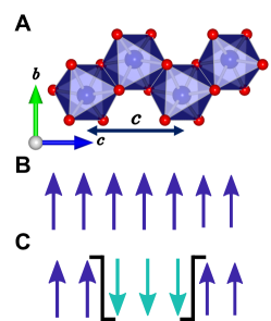
Figure 1: A) A single zigzag chain in CoNb2O6. Blue spheres represent Co^2+ ions, red spheres O^2- ions. The crystallographic unit cell length along the chain direction, $c$, is indicated. B) Ground state and C) excited state of a ferromagnetic Ising chain, obtained by reversing a spin cluster in the center. Only the boundaries (solid lines) cost energy, and they are the left and right solitons respectively. A spin-flip neutron scattering process creates such a pair of left and right solitons.

In this work, we present high resolution single crystal inelastic neutron scattering (INS) data as a function of low to intermediate transverse field in the ordered phase. This regime has also been explored by THz spectroscopy [16], which probe the zone-centre ($\mathbf{Q}=0$) excitations. The INS data reveal a rich evolution of the magnetic spectrum with increasing field: the spectrum splits into three parts with each part behaving very differently. The top two parts are sharp modes, with the top mode becoming progressively flatter and the middle one progressively more dispersive in field, while the lowest energy part is a continuum where the intensity moves from bottom to top upon increasing field.

We seek to understand this rich behaviour in terms of a recently refined Hamiltonian model for CoNb2O6, which proposed all relevant additional exchange terms down to 2% of the Ising exchange [17]. We find that the experimental data agree very well with the results obtained using numerical exact diagonalization (ED) calculations for this full Hamiltonian, where interchain coupling effects are treated in a mean field approximation. To obtain a physical understanding of the spectrum, we start from a picture of soliton quasiparticles, which hop due to both the applied transverse field and the off-diagonal exchange. The competition between these hopping effects leads to soliton hopping terms that alternate along the two legs of the zigzag chain, resulting in two bands with dispersions that are tuned by the applied field. The relevance of a model with alternating hopping of solitons for explaining features in THz spectroscopy data obtained on CoNb2O6 was already mentioned in [16], where solitons were treated as non-interacting. Here we take into account fully the interactions between solitons as we find that this is crucial for a full understanding of the observed spectrum. A spin-flip neutron scattering process creates two-soliton excitations (Fig. 1C), which interact via hard-core repulsion and various nearest-neighbour interaction terms. We solve a minimal model in the two-soliton subspace and find three continua and up to three bound states depending on the values of the Hamiltonian parameters. To understand the character of these bound states, we first focus on the limit where solitons are localized due to the hopping term on alternate bonds being zero, a theoretical situation not previously explored. In this limit, novel bound states arise due to hard core repulsion. We then perturb away from this limit in first order perturbation theory, obtaining analytic expressions for the dispersions and intensities in INS, which give strong qualitative agreement with the data. The results indicate that this regime is indeed realized in CoNb2O6 at intermediate transverse field.

The rest of this paper is organized as follows: Sec. II provides details of the inelastic neutron scattering experiments while Sec. III introduces the model Hamiltonian and provides a qualitative overview of the experimental results. In Sec. IV, we solve the model Hamiltonian in first order perturbation theory in the two-soliton subspace. In Sec. V, we provide a physical picture of the spectrum by starting from the limit where individual solitons are localized and perturbing around this limit. Sec. VI contains our conclusions, and the Appendices give further technical details of the calculations.

II Experimental details

Inelastic neutron scattering measurements of the magnetic excitations were performed on a large single crystal (6.76 g) of CoNb2O6 grown using a floating-zone technique [18] and already used in previous INS experiments [5]. The magnetic field was applied along the crystallographic $b$-direction, which is transverse to the local Ising axis of all the spins. The measurements were performed using the indirect geometry time-of-flight spectrometer OSIRIS at the ISIS facility. OSIRIS was operated with PG(002) analyzers to measure the inelastic scattering of neutrons with a fixed final energy of $E_{f}=1.82$ meV as a function of energy transfer and wavevector transfer in the horizontal $(h0l)$ scattering plane. Throughout this paper, we express the wavevector transfer in the inelastic neutron scattering experiments as $\mathbf{Q}=(2\pi h/a,0,2\pi l/c)$ where $(h,0,l)$ are expressed in reciprocal lattice units of the orthorhombic structural unit cell, with lattice parameters ${a=14.1337}$ Å, $b=5.7019$ Å  and $c=5.0382$ Å  at 2.5 K [13]. The sample was attached to the cold finger of a dilution refrigerator inside a vertical 7.5 T cryomagnet and measurements were taken at a temperature of 0.1 K. The average counting time at each field was around 7 hours.

For each field, two sample orientations were measured ($c$-axis oriented in the scattering plane at 25^∘ and 60^∘ with respect to the incident beam direction). Throughout this paper, the data panels presented are a combination of data from these two orientations, with the wavevector projected along the chain direction $l$ as the physics considered is one-dimensional. The two orientations were chosen such that the projected $l$ values covered a large part of the Brillouin zone along the chain direction. The INS data at one of the measured fields (2.5 T, in Fig. 2Q) was briefly reported in [15].

The data shown have had an estimate of the non-magnetic background subtracted off, and have then been divided by the squared isotropic Co^2+ magnetic form factor $f^{2}(\mathbf{Q})$ and by the neutron polarization factor. The latter was calculated under the assumption that all inelastic scattering is in the polarizations perpendicular to the Ising ($z$) axes and that the dynamical structure factor satisfies $S^{xx}(\mathbf{Q},\omega)=S^{yy}(\mathbf{Q},\omega)$, an approximation which is found to be valid to a large extent for the model Hamiltonian (3) in the low transverse field regime. Here,

$$S^{xx}(\mathbf{Q},\omega)=\sum_{\lambda_{f}}|\langle\lambda_{f}|S^{x}(\mathbf{Q})|\text{GS}\rangle|^{2}\delta(E_{\lambda_{f}}-\hbar\omega),$$ (1)

where the sum extends over all excited states $|\lambda_{f}\rangle$ of energy $E_{\lambda_{f}}$ relative to the ground state $|\text{GS}\rangle$ and where $S^{x}(\mathbf{Q})=\sum_{j}\exp(i\mathbf{Q}\cdot\mathbf{r}_{j})S^{x}_{j}$, with $j$ running over all sites. Under the above assumption, the wavevector dependence of the neutron polarization factor is

$$\mathscr{P}(\mathbf{Q})=1+\frac{\left(\frac{2\pi h}{a}\right)^{2}\sin^{2}{\gamma}+\left(\frac{2\pi l}{c}\right)^{2}\cos^{2}{\gamma}}{\mathbf{Q}^{2}}.$$ (2)

Dividing the raw inelastic neutron scattering intensities by $\mathscr{P}(\mathbf{Q})f^{2}(\mathbf{Q})$ then gives $S^{xx}(\mathbf{Q},\omega)$ up to an overall scale factor. Eq. (2) is appropriate for the experimentally observed zero-field magnetic structure of CoNb2O6 and takes into account the two different chains per crystallographic unit cell with Ising directions at an angle of $\pm\gamma$ to the $c$-direction in the $ac$-plane. We have taken $\gamma$ to be 30^∘[13].

III Evolution of the magnetic excitations with applied field

In this section, we first introduce the model Hamiltonian and relate this to the zero field spectrum, introducing the concept of two-soliton states. In applied field, the spectrum splits into three components with different evolution in field. We show in the following sections that this rich behaviour can be naturally understood in a picture of solitons with dispersions tuned by the transverse field.

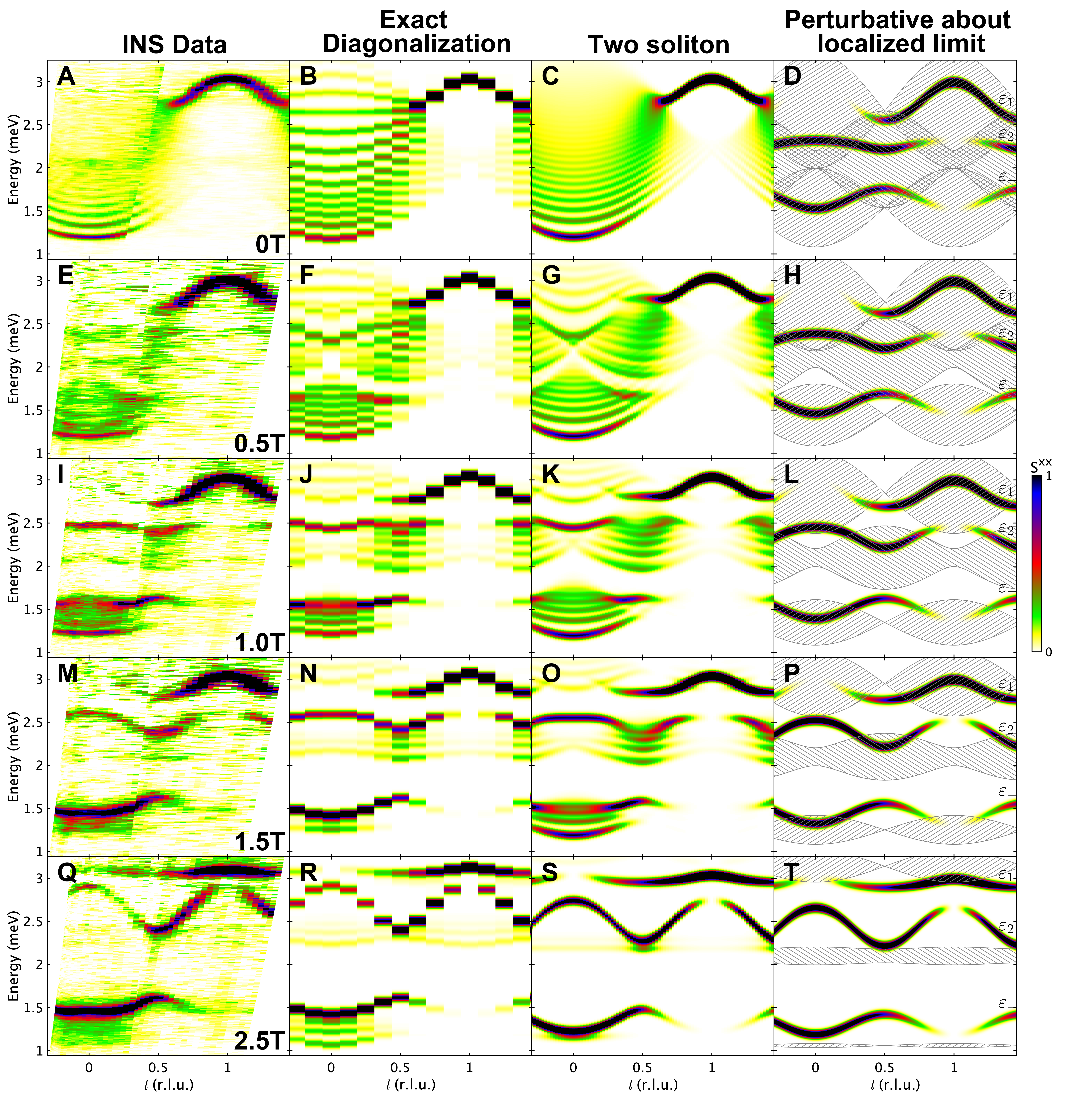
Figure 2: Evolution of the INS spectrum and calculated spectrum for the full Hamiltonian in (3), as a function of applied magnetic field, increasing from top to bottom. Columns left to right: Inelastic neutron scattering data (A adapted from [5]); $S^{xx}$ as calculated by ED on 16 sites (8 unit cells) with periodic boundary conditions; $S^{xx}$ as calculated by diagonalization of the two-soliton subspace (see Sec. IV.2) on 100 sites (50 unit cells) with periodic boundary conditions; $S^{xx}$ as calculated analytically by perturbing about the localized limit for $\lambda_{\text{MF}}$=0 (see Sec. V). In the right-most column, the hatched patches represent the two-soliton continua; in this approximation, the continua have no scattering intensity except where the bound states overlap them and create a resonance. In each panel, color indicates $S^{xx}$, as defined in (1) and further normalized by the total number of sites, on a linear scale indicated by the colorbar. The calculations have been convolved with a Gaussian of FWHM $0.067$ meV to mimic the estimated experimental resolution effects and calculated intensities are shown in absolute units of meV^-1. The intensities for the data in panels E, I, M, Q, have been multiplied by a common scale factor to bring them visually into agreement with the corresponding calculations in column 2. The data in A come from a different experiment so a separate scale factor was used for those intensities to bring them into agreement with those in panel B.

III.1 Model Hamiltonian

We use the single-chain Hamiltonian model for CoNb2O6 recently refined in [17]. It is convenient to write this in three parts:

$$\mathcal{H}=\mathcal{H}_{1}+\mathcal{H}_{2}+\mathcal{H}_{3}$$ (3)

where

$$\mathcal{H}_{1}=J \sum_{j}\left[-S_{j}^{z}S_{j+1}^{z}-\lambda_{S}\left(S_{j}^{x}S_{j+1}^{x}+S_{j}^{y}S_{j+1}^{y}\right)\right.$$

$$+ \left.(-1)^{j}\lambda_{yz}\left(S_{j}^{y}S_{j+1}^{z}+S_{j}^{z}S_{j+1}^{y}\right)\right]+\sum_{j}h_{y}S_{j}^{y},$$ (4)

$$\mathcal{H}_{2}=J \sum_{j}\left[-\lambda_{A}\left(S_{j}^{x}S_{j+1}^{x}-S_{j}^{y}S_{j+1}^{y}\right)\right.$$

$$+ \left.\lambda_{\text{AF}}S_{j}^{z}S_{j+2}^{z}+\lambda_{\text{AF}}^{xy}\left(S_{j}^{x}S_{j+2}^{x}+S_{j}^{y}S_{j+2}^{y}\right)\right],$$ (5)

and

$$\mathcal{H}_{3}=J \sum_{j}2\lambda_{\text{MF}}\left(\langle S^{y}\rangle S^{y}_{j}-\langle S^{z}\rangle S^{z}_{j}\right),$$ (6)

and where $z$ is the Ising direction (in the crystallographic $ac$ plane, defined as the direction of the moments in zero applied field), $y$ is parallel to the crystallographic $b$-direction and $x$ completes a right-handed coordinate system.

This Hamiltonian, with parameter values in Table 1, is a refinement of the minimal model proposed in Ref. [15] and was recently deduced using a simultaneous fit to the spectrum in zero field, large transverse field, and large near-longitudinal field [17]. One can regard $\mathcal{H}_{1}$ as the minimal Hamiltonian needed to qualitatively reproduce all key features of the excitation spectrum, while the terms in $\mathcal{H}_{2}$ are sub-leading and are added in order to achieve quantitative agreement. This applies to both the data in Ref. [17] as well as data in low transverse field presented here. Finally, $\mathcal{H}_{3}$ captures the effects of the weak interchain interactions at a mean-field level. The given form with a constant $\lambda_{\text{MF}}>0$ applies throughout the field range explored here (0 to $2.5$ T $\parallel b$) as the magnetic order pattern between chains does not change in this field range [19] and as, for this magnetic structure, all the interchain interactions that have a net contribution to the mean field are Heisenberg-like [17]. The different signs in front of the $S_{j}^{y}$ and $S_{j}^{z}$ terms reflect the fact that the $S^{y}$-components of spins on neighbouring chains are parallel (polarized by the applied field $h_{y}$), whereas the $S^{z}$ components are (spontaneously) aligned antiparallel by the antiferromagnetic interchain interactions.

The dominant term in the model Hamiltonian is the first term in $\mathcal{H}_{1}$, the nearest neighbour ferromagnetic Ising exchange. The second term is a nearest neighbour ferromagnetic XY exchange term ($\lambda_{S}$), which causes single spin flips to hop. The third term is a staggered off-diagonal exchange term ($\lambda_{yz}$) which causes solitons to hop with a sign that alternates along the legs of the zigzag chain. The transverse field term ($h_{y}=g_{y}\mu_{B}B_{y}$) flips single spins; for a fixed number of domain walls, this is equivalent to soliton hopping by one site. We will show that the competition between these two one-soliton hopping terms leads to a rich field-dependent spectrum.

The spectrum in zero field (Fig. 2A data, 2B calculation) can be qualitatively understood in terms of the minimal Hamiltonian $\mathcal{H}_{1}+\mathcal{H}_{3}$. A spin-flip neutron scattering event creates a pair of solitons (domain walls) and for the pure Ising chain, the energy is independent of the separation between these solitons [see Fig. 1C]. In the presence of the staggered off-diagonal exchange ($\lambda_{yz}$), the solitons become dispersive [15], resulting in a continuum of scattering in energy-momentum space, covering a large energy extent near $l=0$. A longitudinal interchain mean field ($\mathcal{H}_{3}$) acts as an effective linear potential confining the solitons into a series of bound states, as seen in Fig. 2A near $l=0$. The sharp mode in the data near $l=1$ is a two-soliton kinetic bound state stabilized by the XY ($\lambda_{S}$) exchange [5].

The terms in $\mathcal{H}_{2}$ do not change the qualitative content of the spectrum but are important for quantitative agreement with the experimental data. The first term in $\mathcal{H}_{2}$ is an antisymmetric diagonal nearest neighbour exchange ($\lambda_{A}$). The second and third terms are a next nearest neighbour antiferromagnetic XXZ exchange ($\lambda_{\text{AF}}$ and $\lambda_{\text{AF}}^{xy}$ respectively). The second term is needed to account for the energy of the kinetic bound state near $l=1$ [5], while the first and third are needed to explain the details of the dispersions seen in very high field [17]. Fig. 2B demonstrates that very good quantitative agreement has been achieved between the experimental zero-field data and exact diagonalization calculations using the full Hamiltonian (3).

$J$	$2.48(2)\text{~{}meV}$
$\lambda_{S}$	$0.251(6)$
$\lambda_{yz}$	$0.226(3)$
$g_{y}$	$3.32(2)$
$\lambda_{A}$	$-0.021(1)$
$\lambda_{AF}$	$0.077(3)$
$\lambda_{AF}^{xy}$	$0.031(1)$
$\lambda_{\text{MF}}$	$0.0158(2)$

Table 1: Hamiltonian parameters used in (4)-(6), from Ref. [17]

III.2 Spectrum in small to intermediate transverse field

The key feature of the evolution of the spectrum as a function of field, shown in the first column of Fig. 2, is the break-up of the observable spectrum into three parts, each evolving very differently upon increasing field. The top part, which evolves out of the zero-field high-energy kinetic bound state, is a sharp mode that becomes progressively flatter upon increasing field and spreads out over the whole Brillouin zone. In contrast, the middle part is dominated by a sharp mode that becomes progressively more dispersive upon increasing field and appears to trade intensity with the top mode. The lowest energy part is dominated by a continuum spread, with intensity moving from bottom to top upon increasing field. All features and trends in the INS data are quantitatively captured by exact diagonalization (ED) calculations using the full Hamiltonian in (3) with the expectation values $\langle S^{y}\rangle$ and $\langle S^{z}\rangle$ in the mean-field term ${\cal H}_{3}$ calculated self-consistently; these calculations are shown in the second column of Fig. 2.

The breakup of the spectrum in field is clearly illustrated in Fig. 2I at 1 T. The lowest energy part of the spectrum centred around $1.4~{}$meV shows a set of excitations extending over a broad energy range with clear sharp modes visible both at the bottom and the top of this range. Those excitations are clearly separated from another set of states centred around $2.25$ meV with a clear sharp mode near $2.5$ meV. At higher energies still, there is the vestige of the zero-field kinetic bound state near $l=1$, now clearly separated from the rest of the spectrum. All the observed features, both dispersions and wavevector-dependence of intensities, are well captured by the ED calculations in Fig. 2J.

The 2.5 T data (Fig. 2Q) shows even more contrasting behaviour between the different parts of the spectrum. The sharp mode at the top of the low energy continuum now extends all the way from the Brillouin zone center to $l\approx 0.6$ and has gained in intensity compared to the continuum below it. In the middle energy region the sharp mode has become strongly dispersive, with the middle continuum losing nearly all its scattering intensity, and the top sharp mode has become almost entirely flat and spread out over almost all the Brillouin zone. Again, all these features are well reproduced in Fig. 2R. The spectra at 0.5 T (Figs. 2E and F) and 1.5 T (Figs. 2M and N) interpolate between 0, 1 and 2.5 T and show the gradual evolution of the spectrum.

The ED calculations quantitatively capture every feature and trend described above. We stress that the parameters used in this calculation were not fit to the finite transverse field data presented here, but are fixed to the values proposed in [17]. This excellent agreement between data and calculation gives further support to the Hamiltonian proposed in [17] and motivates our search for a physical picture of the excitations. In the following sections, we will introduce a picture of solitons on the zigzag chains and show that the breaking up of the spectrum and very different evolution of the different parts in field can be captured quantitatively and understood phenomenologically in terms of solitons hopping and bound state formation.

IV Two-soliton model

In (4) to (6), all $\lambda$ terms are $\ll 1$ such that the dominant term is the ferromagnetic Ising term. This means that it is sufficient for our purposes to consider two-soliton excitations, and neglect mixing with four-or-more-soliton excitations, since those occur at much higher energy. More systematically, we may write the Hamiltonian as

$$\mathcal{H}=\mathcal{H}_{\rm Ising}+\mathcal{V},$$

with $\mathcal{H}_{\rm Ising}$ denoting the Ising Hamiltonian, and $\mathcal{V}$ containing all other terms in $\mathcal{H}$. We now treat $\mathcal{V}$ as a perturbation of order $\delta$, and define a Schrieffer-Wolff transformation,

$$\mathcal{H}^{\prime}=e^{\mathcal{S}}\mathcal{H}e^{-\mathcal{S}},$$

with $\mathcal{S}^{\dagger}=-\mathcal{S}$. We require that

$$[\mathcal{H}^{\prime},\mathcal{H}_{\rm Ising}]=0,$$ (7)

i.e., that $\mathcal{H}^{\prime}$ conserves the number of solitons (domain walls). By expanding $\mathcal{S}=\mathcal{S}_{1}\delta+\mathcal{S}_{2}\delta^{2}+...$, and enforcing (7) up to order $\delta^{n}$ with $n\in\mathbb{Z}^{+}$, we obtain a systematic perturbative series for the effective Hamiltonian within subspaces with a fixed number of solitons. Up to lowest order in $\delta$, we arrive at

$$\mathcal{H}^{\prime}\approx\mathcal{H}_{\rm Ising}+\mathcal{V}_{\rm conserv}=\sum_{i\geq 0}\mathcal{P}_{i}\mathcal{H}\mathcal{P}_{i},$$ (8)

with $\mathcal{V}_{\rm conserv}$ denoting the soliton number conserving terms in $\mathcal{V}$, and $\mathcal{P}_{i}$ standing for the projector to the sector with exactly $i$ solitons. We have verified that the second order terms, $\sim\delta^{2}$, are negligible compared to this leading contribution.

Relying on these insights, we now start by considering the effect of the effective Hamiltonian  (8), first on a single soliton, and then within the two-soliton sector. We focus on the minimal Hamiltonian $\mathcal{H}_{1}+\mathcal{H}_{3}$, yielding a good qualitative understanding of the spectrum, and leave the discussion of $\mathcal{H}_{2}$ to the Appendices. We further assume that the most important contribution from the mean field interchain coupling $\mathcal{H}_{3}$ is a $z$ magnetic field,

$$\mathcal{H}_{3}\approx-h_{z}\sum_{j}S_{j}^{z},\quad{\rm with}\;h_{z}=2J\lambda_{\rm MF}\langle S^{z}\rangle\approx J\lambda_{\rm MF},$$

assuming $\langle S^{z}\rangle=1/2$. For convenience, we define the unconventional raising and lowering operators,

$$S_{j}^{\pm}=S_{j}^{y}\mp iS_{j}^{x},$$ (9)

which obey the usual commutation relations. Note that this is equivalent to performing the calculations in a spin basis rotated by $\pi/2$ around the $z$ axis, obtained via the canonical transformation $S^{x}_{j}\rightarrow-S^{y}_{j}$ and $S^{y}_{j}\rightarrow S^{x}_{j}$ in $\mathcal{H}$.

IV.1 Action of the Hamiltonian on a single soliton

In this section we consider the spectrum of deconfined solitons under the Hamiltonian $\mathcal{H}_{1}$ projected to the single soliton sector. The confining mean field $\mathcal{H}_{3}$ will be introduced in Sec. IV.2, where we discuss the spectrum in the two-soliton sector.

Let us define the “left” soliton state, a single domain wall at the link $(j-1,j)$, separating up spins on the left and down spins on the right,

$$|j\rangle_{L} =\left|\cdots\uparrow\uparrow\uparrow_{j-1}\downarrow_{j}\downarrow\downarrow\cdots\right\rangle.$$ (10)

Here, the arrows indicate the eigenstates of $S_{j}^{z}$ with eigenvalues $\pm 1/2$. We now consider the action of the Hamiltonian $\mathcal{H}_{1}$ on this state, term by term.

• Ising exchange: The single soliton state $|j\rangle_{L}$ is an eigenstate, with excitation energy $\epsilon_{0}=J/2$ above the ground state.

• XY exchange $\lambda_{S}$: This term flips two adjacent spins in opposite directions. Acting on $|j\rangle_{L}$, it creates two additional domain walls by flipping the spins at sites $j-1$ and $j$, and can therefore be dropped.

• transverse field $h_{y}$: This term flips a single spin,

  $$V_{y}=\dfrac{h_{y}}{2}\sum_{j}\left(S^{+}_{j}+S^{-}_{j}\right),$$

  where we have used the unconventional raising and lowering operators (9). To conserve the number of solitons when acting on $|j\rangle_{L}$, the flipped spin must be either at $j$ or $j-1$,

  $$\mathcal{P}_{1}V_{y}|j\rangle_{L}=\frac{h_{y}}{2}\left(|j+1\rangle_{L}+|j-1\rangle_{L}\right).$$

  Therefore, the transverse field gives rise to a nearest neighbour hopping term for the domain wall.

• staggered off-diagonal exchange $\lambda_{yz}$: Similarly to the transverse field $h_{y}$, this term results in a single spin flip,

  $$V_{yz} =\dfrac{J\lambda_{yz}}{2}\sum_{j}(-1)^{j}\left(S_{j}^{+}+S_{j}^{-}\right)\left(S_{j+1}^{z}-S_{j-1}^{z}\right).$$

  Here, the operator $S_{j}^{+}+S_{j}^{-}$ can flip the spin at site $j$ if and only if the spins on sites $j+1$ and $j-1$ are opposite, due to the factor $S_{j+1}^{z}-S_{j-1}^{z}$. Therefore, $V_{yz}$ yields spin flip processes confined to domain walls. We find

  $$\mathcal{P}_{1}V_{yz}|j\rangle_{L} =\frac{J\lambda_{yz}}{2}(-1)^{j+1}\left(|j+1\rangle_{L}-|j-1\rangle_{L}\right),$$

  a hopping term similar to the effect of the field $h_{y}$, but with a different sign structure across links.

To obtain the spectrum of this hopping Hamiltonian, we write a Schrödinger equation for the soliton. We define the state

$$|\psi_{L}\rangle=\sum_{j^{\prime}}\psi_{L}(j^{\prime})|j^{\prime}\rangle_{L},$$

where $\psi_{L}(j)={}_{L}\langle j|\psi\rangle$ is the wavefunction of the soliton. Using the expressions derived for $\mathcal{P}_{1}\mathcal{H}_{1}|j\rangle_{L}$ above, the Schrödinger equation,

$${}_{L}\langle j|\mathcal{H}_{1}|\psi_{L}\rangle=\omega\,\psi_{L}(j),$$

can be rewritten as

$$\frac{1}{2}\sum_{\Delta=\pm 1}\left(h_{y}+(-1)^{j}J\lambda_{yz}\Delta\right)\psi_{L}(j-\Delta)=\left(\omega-\frac{J}{2}\right)\psi_{L}(j).$$

This equation describes a staggered hopping of solitons, with hopping amplitudes

$$h_{\pm}=\dfrac{1}{2}\left(h_{y}\pm J\lambda_{yz}\right)$$ (11)

alternating on even/odd bonds.

Since $\mathcal{H}$ is invariant under translations by two lattice sites, we can use the following Bloch ansatz,

$$\psi_{L}(2p+\sigma)=\psi_{L\sigma}e^{ikpc},\quad{\rm with}\;\sigma=0,1.$$

where $k=2\pi l/c$ is the soliton momentum. In the following, we will interchangeably use the symbols $k$ and $l$ when referring to momentum along the chain direction, with the only difference that $k$ is in absolute units whereas $l$ is in reciprocal lattice units. In the above equation, the coefficients $\psi_{L\sigma}$ differentiate between the even and odd sublattices, reflecting the two-site unit cell of the Hamiltonian. From now on, we will reserve the index $p$ for labelling the unit cells, whereas $j$ will be used as a label of lattice sites. With this convention, the Schrödinger equation reduces to

$$\left(h_{+}e^{-ikc}+h_{-}\right)\psi_{L1} =\left(\omega-\frac{J}{2}\right)\psi_{L0},$$

$$\left(h_{+}e^{ikc}+h_{-}\right)\psi_{L0} =\left(\omega-\frac{J}{2}\right)\psi_{L1},$$

yielding a pair of bands, $\omega_{\pm}$, with bonding / anti-bonding orbitals

$$\left(\frac{J}{2}-\omega_{\pm}\right)^{2} =\left(h_{+}e^{-ikc}+h_{-}\right)\left(h_{+}e^{ikc}+h_{-}\right)$$

$$=h_{+}^{2}+h_{-}^{2}+2h_{+}h_{-}\cos kc.$$ (12)

Importantly, the dispersion vanishes if $h_{+}=0$ or $h_{-}=0$. In these limits, the hopping amplitude vanishes either on odd or on even bonds, and the domain wall can only move between two sites, giving rise to flat localized bands, as previously noted in [16]. This localized limit will serve as a convenient starting point for perturbative considerations in Sec. V, allowing us to obtain a simple qualitative picture for the evolution of the INS spectrum with magnetic field $h_{y}$.

Above we considered a single “left” soliton, describing a domain wall with up spins on the left and down spins on the right. Another type of domain wall excitation is a “right” soliton, separating a domain of down spins on the left from up spins on the right,

$$|j\rangle_{R}=\left|\cdots\downarrow\downarrow\downarrow_{j-1}\uparrow_{j}\uparrow\uparrow\cdots\right\rangle.$$

The arguments described above can be repeated for right solitons, with the only difference being that the hopping induced by $\lambda_{yz}$ is of opposite sign compared to the case of left solitons. This interchanges the hopping amplitudes $h_{+}$ and $h_{-}$ in the Schrödinger equations, but leaves the dispersion (IV.1) unaltered. Therefore, both solitons become localized at the same critical magnetic field $h_{y}$.

IV.2 Solution of the Hamiltonian in the two-soliton subspace

We now turn to the spectrum of the effective Hamiltonian within the two-soliton subspace. In Sec. IV.1 we obtained two distinct soliton dispersions, $\omega_{\pm}$, describing bonding/anti-bonding orbitals. Therefore, we expect three continua in the two-soliton subspace, arising from the pairings $(\omega_{+},\omega_{+})$, $(\omega_{+},\omega_{-})$ and $(\omega_{-},\omega_{-})$. However, the solitons interact, due both to hard-core repulsion and to nearest neighbour soliton-soliton interactions encoded in $\mathcal{H}_{1}$. Moreover, the full Hamiltonian also includes a confining $z$ magnetic field, $\mathcal{H}_{3}$, yielding an attractive interaction between the two solitons in a pair. Below, we take into account all of these effects by considering $\mathcal{H}_{1}+\mathcal{H}_{3}$ projected to the relevant subspace with $\mathcal{P}_{2}$ and show that a full understanding of the spectrum cannot neglect these interactions.

Assuming $h_{z}>0$, the relevant low energy excitations correspond to a single domain of down spins inserted into a background of up spins. Therefore, it is convenient to use the following basis, with a “left” soliton on the left and a “right” soliton on the right,

$$|j_{L},j_{R}\rangle=\left|\cdots\uparrow\uparrow_{j_{L}-1}\downarrow_{j_{L}}\cdots\downarrow_{j_{R}-1}\uparrow_{j_{R}}\uparrow\cdots\right\rangle,$$

with $j_{L}<j_{R}$. Similarly to the procedure followed in Sec. IV.1, we can derive a Schrödinger equation within the two-soliton subspace by considering the effect of $\mathcal{P}_{2}\mathcal{H}_{1}$ and $\mathcal{H}_{3}$ on the basis states.

The transverse field $h_{y}$ and staggered off-diagonal exchange $\lambda_{yz}$ again give rise to hopping terms for the left and right solitons, with a correction term arising for nearest neighbor solitons $j_{R}=j_{L}+1$ due to hard core repulsion,

$$\mathcal{P}_{2}V_{y}|j_{L},j_{R}\rangle=\frac{h_{y}}{2}\sideset{}{{}^{\prime}}{\sum}_{\Delta=\pm 1}\left(|j_{L}+\Delta,j_{R}\rangle+|j_{L},j_{R}+\Delta\rangle\right),$$

and

$$\mathcal{P}_{2}V_{yz}|j_{L},j_{R}\rangle=$$

$$\frac{J\lambda_{yz}}{2}\sideset{}{{}^{\prime}}{\sum}_{\Delta=\pm 1}\Delta\left((-1)^{j_{L}}|j_{L}-\Delta,j_{R}\rangle-(-1)^{j_{R}}|j_{L},j_{R}-\Delta\rangle\right).$$

Here $\sideset{}{{}^{\prime}}{\sum}$ denotes a restricted summation constrained to valid basis states, by dropping the unphysical terms $|j_{L}+1,j_{R}\rangle$ and $|j_{L},j_{R}-1\rangle$ for neighboring solitons $j_{R}=j_{L}+1$.

Besides these familiar terms, two new types of contributions arise compared to the single soliton case. The XY exchange term,

$$V_{S}=\frac{-J\lambda_{S}}{2}\sum_{j}\left(S_{j}^{+}S_{j+1}^{-}+S_{j}^{-}S_{j+1}^{+}\right),$$

gives rise to a nearest neighbor interaction term between solitons,

$$\mathcal{P}_{2}V_{S}|j_{L},j_{R}\rangle=-\frac{J\lambda_{S}}{2}\delta_{j_{R}-j_{L},1}\sum_{\Delta=\pm 1}|j_{L}-\Delta,j_{R}-\Delta\rangle.$$

This term shifts the center of mass coordinate of the soliton pair by one lattice site, without changing the relative coordinate $j_{R}-j_{L}$. Finally, the magnetic field $h_{z}$ leads to an attractive potential between the left and right soliton,

$$\mathcal{H}_{3}|j_{L},j_{R}\rangle=h_{z}(j_{R}-j_{L})|j_{L},j_{R}\rangle.$$

Based on these relations, we construct the two-particle Schrödinger equation for the wavefunction $\Psi(j_{L},j_{R})$ defined through

$$|\Psi\rangle=\sum_{j_{L}<j_{R}}\Psi(j_{L},j_{R})|j_{L},j_{R}\rangle.$$

Relying on translational invariance for the center of mass coordinate, it is convenient to write

$$\Psi(2p_{L}+\sigma_{L},2p_{R}+\sigma_{R})=e^{ikc(p_{L}+p_{R})/2}\Phi_{\sigma_{L}\sigma_{R}}^{(k)}(p_{R}-p_{L}),$$ (13)

with $p_{L/R}$ labeling the two site unit cells, $\sigma_{L/R}=0,1$ distinguishing the even and odd sublattice and ${c(p_{L}+p_{R})/2}$ being the position of the center of mass of the soliton pair. For a fixed center of mass momentum $k$, we obtain coupled equations for $\Phi_{\sigma_{L}\sigma_{R}}^{(k)}(n)$, defined on the half line $n\geq 0$ with boundary conditions $\Phi_{00}^{(k)}(0)=\Phi_{11}^{(k)}(0)=\Phi_{10}^{(k)}(0)=0$. We present more details on the numerical solution of these equations in Appendix A.

The two-soliton Schrödinger equation derived above yields a spectrum consisting of three continua and three bound states across a wide range of parameters, see Appendix C. As mentioned above, the origin of the three continua can be understood as due to the three different ways of combining the two bands of solitons into two-soliton continua. The origin of the bound states, which we term $\varepsilon$ bound states to avoid confusion, will be explored in the following section, Sec. V.

Before turning to the detailed study of the $\varepsilon$ bound states, we conclude this section by deriving a formula for the INS spectrum within the two-soliton model, showing that the dominant contribution stems from the three bound states. To this end, we approximate the ground state $|\text{GS}\rangle$ appearing in the dynamical structure factor $S^{xx}$, Eq. (1), as the ground state of the Ising Hamiltonian, $|\text{GS}\rangle\approx|...\uparrow\uparrow\uparrow...\rangle$. Acting with the spin operator $S^{x}(k)$ creates a soliton pair. Using the unconventional raising and lowering operators $S_{j}^{\pm}=S_{j}^{y}\mp iS_{j}^{x}$, we can write the resulting state as

$$S^{x}(k)|\text{GS}\rangle\approx-\dfrac{i}{2}\sum_{j}e^{ikjc/2}|j,j+1\rangle,$$

where $k=2\pi l/c$ is the soliton pair center of mass momentum. By substituting the eigenstates $|\lambda_{f}\rangle$ with the solutions of the two-soliton Schrödinger equation constructed above, we arrive at the overlaps

$$|\langle\lambda_{f}|S^{x}(k)|\text{GS}\rangle|^{2}\sim\left|\Phi_{01}^{(k)}(0)+\Phi_{10}^{(k)}(1)\right|^{2}.$$ (14)

Therefore, the $\varepsilon$ bound states, which we will show to have a large weight on the configurations with nearest neighbor domain walls, give the dominant contribution to the dynamical spin structure factor (1).

The INS intensity as calculated above is shown in the third column of Fig. 2. The calculation uses the full Hamiltonian with the same parameters as in the ED calculations, except that the spin vector expectation value $\langle\mathbf{S}\rangle=(0,0,1/2)$ is assumed fixed, rather than using a self-consistent value. This is a good approximation since even at 2.5 T, the self-consistent value as calculated by ED is $\langle\mathbf{S}\rangle=(0,-0.150,0.473)$. The agreement between the observed spectrum and the model is still quantitative — all features and trends are captured — but not quite as strong as for the exact diagonalization calculation. For instance, there is a small overall energy shift, most visible by comparing Figs. 2R and S; in the latter, energies are shifted to lower values. However all key features are well reproduced at all measured fields.

To gain more insight into the structure and magnetic field dependence of this INS signal, we examine the $\varepsilon$ bound states in the next section, by relying on a perturbative argument around the localized limit $h_{-}=0$.

V The localized limit

As derived in Sec. IV.1, the staggered off-diagonal exchange $\lambda_{yz}$ and the transverse field $h_{y}$ in the leading order Hamiltonian $\mathcal{H}_{1}$ lead to hopping terms of opposite sign for the solitons. A particularly interesting situation arises when these terms are matched, such that $h_{-}=0$, resulting in localized single solitons. This localized limit serves as a convenient starting point for perturbative considerations, shedding light on the structure and magnetic field dependence of the $\varepsilon$ bound states, as well as the three two-soliton continua. First, in Sec. V.1, we set $h_{-}=0$, and study the two-soliton spectrum, in particular, the nature of the two-soliton bound states. We then examine the effect of a small non-zero delocalizing term $h_{-}$ in Sec. V.2. Predictions for the evolution of the INS spectra with decreasing transverse field $h_{y}$, and comparisons of these to the experimental data, are discussed in Sec. V.3. For most of this section, we focus on the leading order Hamiltonian $\mathcal{H}_{1}$, with a brief comment about the mean field $\mathcal{H}_{3}$ at the end of the section.

V.1 Localized limit $h_{-}=0$

For simplicity, we start by setting $\lambda_{S}=0$ as well, and only keep the staggered off-diagonal exchange $\lambda_{yz}$ and the transverse field $h_{y}$. We will discuss the effect of the nearest neighbor exchange $\lambda_{S}$ later. Under these simplifications, a left soliton can hop between the two sites of a unit cell $p$, $2p\leftrightarrow 2p+1$, with rate $h_{-}$, whereas it hops between neighboring unit cells $p-1$ and $p$, through sites $2p-1\leftrightarrow 2p$, with rate $h_{+}$, see Fig. 3A. For $h_{-}=0$, we obtain the following eigenstates with energies $\omega_{\pm}$,

$$|p\rangle_{L}^{\pm}\equiv\dfrac{1}{\sqrt{2}}\left(|2p-1\rangle_{L}\pm|2p\rangle_{L}\right),\quad\omega_{\pm}=\frac{J}{2}\pm h_{+},$$

symmetric and antisymmetric under the inversion exchanging the even and odd sublattices, respectively. For a right soliton, the role of $h_{-}$ and $h_{+}$ is interchanged, leading to symmetric / antisymmetric eigenstates localized within a single unit cell $p$,

$$|p\rangle_{R}^{\pm}\equiv\dfrac{1}{\sqrt{2}}\left(|2p\rangle_{R}\pm|2p+1\rangle_{R}\right),\text{ with }\omega_{\pm}=\frac{J}{2}\pm h_{+}.$$

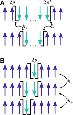
Figure 3: Soliton hopping in the localized limit. A) In the case of well separated solitons, they can hop independently, with each soliton hopping between two sites with matrix element $h_{+}$. B) When solitons are in adjacent unit cells, hopping is constrained by hard-core repulsion between solitons.

Relying on these observations, we can construct the localized two-soliton eigenstates by considering a left soliton confined to sites $2p-1$ and $2p$, and a right soliton on $2p^{\prime}$ and $2p^{\prime}+1$. For $p^{\prime}>p$, the solitons do not interact, and we obtain the eigenstates

$$|p\rangle_{L}^{-}\otimes|p^{\prime}\rangle_{R}^{-},\text{ with energy }\omega_{--}=J-2h_{+},$$

$$\dfrac{1}{\sqrt{2}}\left[|p\rangle_{L}^{+}\otimes|p^{\prime}\rangle_{R}^{-}\pm|p\rangle_{L}^{-}\otimes|p^{\prime}\rangle_{R}^{+}\right],\text{ with }\omega_{+-}=J,$$

$$|p\rangle_{L}^{+}\otimes|p^{\prime}\rangle_{R}^{+},\text{ with }\omega_{++}=J+2h_{+}.$$

The eigenvalue $\omega_{+-}=J$ is doubly degenerate, and the eigenstates were chosen to be symmetric / antisymmetric under inversion. We now construct delocalized eigenstates with a well defined center of mass momentum $k$ as follows

$$|n,k\rangle^{\pm}=\dfrac{1}{\sqrt{N}}\sum_{\text{cells},p}e^{ikc(2p+n)/2}|p\rangle_{L}^{\pm}\otimes|p+n\rangle_{R}^{\pm},$$

$$|n,k\rangle^{0}_{\pm}=\dfrac{1}{\sqrt{2N}}\sum_{\text{cells},p}e^{ikc(2p+n)/2}\left(|p\rangle_{L}^{+}\otimes|p+n\rangle_{R}^{-}\right.$$

$$\qquad\qquad\qquad\qquad\qquad\quad\left.\pm|p\rangle_{L}^{-}\otimes|p+n\rangle_{R}^{+}\right),$$ (15)

with $N$ denoting the number of unit cells, and $n\geq 1$. These eigenstates correspond to the three two-soliton continua arising from the different pairing of bonding / anti-bonding orbitals. In the localized limit considered here, we obtain highly degenerate flat bands at energies $J\pm 2h_{+}$ and $J$, reflected by the free index $n$ standing for the relative coordinate between the left and right solitons.

Placing the left soliton to sites $2p-1$ and $2p$, and the right soliton to $2p^{\prime}$ and $2p^{\prime}+1$ with $p=p^{\prime}$ gives rise to interaction through hard core repulsion, see Fig. 3B. In this case, the eigenstates can be obtained by diagonalizing a $3\times 3$ matrix acting on the three allowed configurations, yielding

$$|\varepsilon_{\pm},p\rangle=\dfrac{1}{2}\left(|2p-1,2p\rangle+|2p,2p+1\rangle\right.$$

$$\hskip 85.35826pt\left.\pm\sqrt{2}|2p-1,2p+1\rangle\right),$$

$$|\varepsilon_{0},p\rangle=\dfrac{1}{\sqrt{2}}\left(|2p-1,2p\rangle-|2p,2p+1\rangle\right),$$

with energies $\varepsilon_{\pm}=J\pm\sqrt{2}h_{+}$ and $\varepsilon_{0}=J$. The corresponding momentum eigenstates form non-degenerate flat bands (Fig. 4A) given by

$$|\varepsilon_{\alpha},k\rangle=\dfrac{1}{\sqrt{N}}\sum_{\text{cells},p}e^{ikpc}|\varepsilon_{\alpha},p\rangle,\text{ for }\alpha=\pm,0.$$ (16)

These states are the origin of the $\varepsilon$ bound states found through the numerical solution of the two-soliton Schrödinger equation in Sec. IV.

We now consider the effect of a weak symmetric exchange $\lambda_{S}$, while keeping $h_{-}=0$. As discussed in Sec. IV, this term only affects nearest neighbor solitons by shifting the center of mass coordinate. Therefore, the three continua, (V.1), with solitons residing in different unit cells are not affected. In contrast, the symmetric exchange acts non-trivially on the bound states  (16), inducing an energy shift calculated perturbatively as

$$\varepsilon_{\alpha}\longrightarrow\varepsilon_{\alpha}(k)\approx\varepsilon_{\alpha}+\langle\varepsilon_{\alpha},k|\,V_{S}\,|\varepsilon_{\alpha},k\rangle,$$

yielding dispersive bands

$$\varepsilon_{\pm}(k)=J\pm\sqrt{2}h_{+}-\dfrac{J\lambda_{S}}{4}\left(1+\cos{kc}\right),$$

$$\varepsilon_{0}(k)=J+\dfrac{J\lambda_{S}}{2}\left(1+\cos{kc}\right).$$ (17)

The full spectrum of the localized limit $h_{-}=0$, with weak symmetric exchange $\lambda_{S}$ is illustrated in Fig. 4B, showing the three highly degenerate flat continua, and the three dispersive $\varepsilon$ bound states, which become delocalized by $\lambda_{S}$. Note that in CoNb2O6, $\lambda_{S}$ is large enough that the dispersion causes the $\varepsilon_{0}$ and $\varepsilon_{+}$ bands to cross, leading to band inversion. This effect is discussed quantitatively in Appendix D and illustrated in Fig. 4C. The band inversion further suppresses the dispersion of the top mode, as well as mixing the character of the two bands.

V.2 Effects of weak delocalizing hopping $h_{-}$

Figure 4: Dispersions and intensities as a function of wavevector and energy at different stages of perturbation away from the purely localized limit. The $x$-axis is momentum in reciprocal lattice units, $l=kc/(2\pi)$, vertical axis is energy relative to $J$. In each panel, color indicates $S^{xx}$, as defined in (1) and further normalized by the total number of sites, on a linear scale indicated by the colorbar; black lines represent $\varepsilon$ bound states while gray hatched patches represent continua. The calculated intensities have been convolved with a Gaussian of FWHM $0.033J$ and are shown in absolute units of $1/J$. In all panels, $h_{+}=0.2J$. In A-D) the calculation uses the perturbative regime of Sec. V. A) Bound states and continua are both dispersionless for $h_{-}=0$ and $\lambda_{S}=0$. B) For finite $\lambda_{S}$, bound states become dispersive but continua remain flat and highly degenerate. C) Band inversion occurs between the top two bound states $\varepsilon_{+}$ and $\varepsilon_{0}$ for $J\lambda_{S}>2\sqrt{2}h_{+}/3$ (see Appendix D), resulting in modes labelled $\varepsilon_{1,2}$, such that $\varepsilon_{1}$ inherits the structure of the state $\varepsilon_{0}$ close to $l=0$ and $l=1$ while retaining the character of $\varepsilon_{+}$ elsewhere, with $\varepsilon_{2}$ showing the opposite behavior. This is reflected by the change in intensity distribution from B to C near $l=0,1$. D) Continua become dispersive for finite $h_{-}$. E) Same as D, but calculated using the full two-soliton model in Sec. IV, which predicts hybridization between the lowest two bound states, $\varepsilon_{2}$ and $\varepsilon_{-}$, and the continua they overlap.

As shown above, the localized limit $h_{-}=0$ provides remarkable insight into the structure of the two-soliton spectrum obtained near to this limit. We can gain a more detailed understanding of the evolution of the spectrum with decreasing transverse field by considering the effect of a weak delocalizing hopping term $h_{-}$ perturbatively. The first important effect of $h_{-}\neq 0$ is lifting the high degeneracy of the three continua and broadening these bands. Secondly, a finite $h_{-}$ can mix the $\varepsilon$ bound states constructed in the previous section with the continua in $k$ regions where they overlap in energy.

We first explore the first effect, by focusing on the continua, and applying degenerate perturbation theory within each band separately. We note that for weak $h_{-}$ and $\lambda_{S}$, the bottom and top bands remain well separated from the $\varepsilon$ bound states. Assuming also $\lambda_{S}\gg h_{-}$, the middle continuum overlaps with the middle bound state only in the vicinity of $k=\pi/c$, see Fig. 4D. Therefore, our treatment of neglecting the hybridization between the continua and the $\varepsilon$ bound states is justified in the limit of weak couplings $h_{+}\gg\lambda_{S}\gg h_{-}$, apart from the case of the middle band in the vicinity of $k=\pi/c$. While the experimental parameters lie outside of this well controlled region, we will demonstrate below that a first order perturbative expansion grants valuable insight into the evolution of the INS spectra for the whole range of applied transverse fields.

Denoting the hopping term by $V_{h_{-}}$, we find that the matrix elements between the single soliton eigenstates of the localized limit are

$$_{\alpha}^{\pm}\langle p^{\prime}|V_{h_{-}}|p\rangle_{\alpha}^{\pm}=\pm\dfrac{h_{-}}{2}\left(\delta_{p^{\prime},p+1}+\delta_{p^{\prime},p-1}\right),\;\;\alpha=L,R.$$ (18)

Up to first order in perturbation theory, the energy shifts of the three continua can be evaluated by considering the matrix elements of $V_{h_{-}}$ between the two-soliton eigenstates of the localized limit, (V.1), within each band separately. Relying on the relations (18), we obtain for the top and bottom bands

$${}^{\pm}\langle n^{\prime},k^{\prime}|V_{h_{-}} |n,k\rangle^{\pm}=$$

$$\pm\delta_{k,k^{\prime}}\,h_{-}\cos\left(\frac{kc}{2}\right)\left(\delta_{n,n^{\prime}+1}+\delta_{n,n^{\prime}-1}\right).$$

For a fixed center of mass momentum $k$, this equation corresponds to an effective nearest neighbor hopping Hamiltonian for the relative coordinate $n$, with hopping amplitude $\pm h_{-}\cos(kc/2)$, subject to the hard core constraint $n>0$. Therefore, for the bottom and top bands we find the spectrum,

$$\omega_{\sigma\sigma}=J+2\sigma\left(h_{+}+h_{-}\cos\left(\frac{kc}{2}\right)\cos\left(\frac{qc}{2}\right)\right),\;\;\sigma=\pm 1,$$

with approximate unnormalized eigenstates

$$|q,k\rangle^{\pm}\sim\sum_{\begin{subarray}{c}\text{cell separation},\\ n>0\end{subarray}}\sin\left(\frac{qnc}{2}\right)\,|n,k\rangle^{\pm}.$$

Here, $k$ is the total momentum of the soliton pair and $q$ is the relative momentum of the two solitons, and the factor $\sin(qnc/2)$ reflects hard core repulsion $n>0$. Thus, the weak hopping $h_{-}$ broadens the bands, most strongly around $k=0$, but the high degeneracy still persists at $k=\pi/c$, see Fig. 4D.

Turning to the middle continuum, we have to calculate four types of matrix elements between the two-soliton states $|n,k\rangle_{\pm}^{0}$. We obtain

$${}_{-}^{0}\langle n^{\prime},k^{\prime}|V_{h_{-}}|n,k\rangle_{+}^{0}=\,_{+}^{0}\langle n^{\prime},k^{\prime}|V_{h_{-}}|n,k\rangle_{-}^{0}$$

$$\hskip 56.9055pt=\delta_{k,k^{\prime}}\,i\,h_{-}\sin\left(\frac{kc}{2}\right)\left(\delta_{n^{\prime},n+1}-\delta_{n^{\prime},n-1}\right),$$

$${}_{-}^{0}\langle n^{\prime},k^{\prime}|V_{h_{-}}|n,k\rangle_{-}^{0}=\,_{+}^{0}\langle n^{\prime},k^{\prime}|V_{h_{-}}|n,k\rangle_{+}^{0}=0.$$

We can now calculate the broadening of this band by diagonalizing this matrix within a given total momentum sector $k$. We find that the eigenstates in the middle band remain at least twofold degenerate everywhere, yielding the spectrum

$$\omega_{+-}=J-2h_{-}\sin\left(\frac{kc}{2}\right)\sin\left(\frac{qc}{2}\right),$$

with approximate unnormalized eigenstates

$$|q,k\rangle^{0}_{1}\sim\!\sum_{\begin{subarray}{c}\text{cell separation},\\ n>0\end{subarray}}\!\!\left(e^{iqcn/2}-e^{-i(qc/2+\pi)n}\right)|n,k\rangle^{0}_{\xi(n)},$$

$$|q,k\rangle^{0}_{2}\sim\!\sum_{\begin{subarray}{c}\text{cell separation},\\ n>0\end{subarray}}\!\!\left(e^{iqcn/2}-e^{-i(qc/2+\pi)n}\right)|n,k\rangle^{0}_{\xi(n+1)},$$

with $\xi(n)=\pm$ for $n$ even/odd, and $q$ again standing for the relative momentum. Thus, the middle band remains highly degenerate around $k=0$, but it is broadened away from this point, most strongly around $k=\pi/c$.

We note that these dispersions of the continua can be understood based on the single-soliton spectrum as given in (IV.1). In the limit of small $h_{-}$, (IV.1) becomes

$$\omega_{\pm}=\frac{J}{2}\pm(h_{+}+h_{-}\cos kc).$$ (19)

The three continua constructed above correspond to the three different types of soliton pairs. Denoting the individual solitons’ momenta by $k_{1}$ and $k_{2}$, we obtain the energies

$$\omega_{++}= J+2h_{+}+h_{-}(\cos k_{1}c+\cos k_{2}c)$$

$$= J+2h_{+}+2h_{-}\cos\left(\frac{kc}{2}\right)\cos\left(\frac{qc}{2}\right),$$

$$\omega_{--}= J-2h_{+}-h_{-}(\cos k_{1}c+\cos k_{2}c)$$

$$= J-2h_{+}-2h_{-}\cos\left(\frac{kc}{2}\right)\cos\left(\frac{qc}{2}\right),$$

$$\omega_{+-}= J+h_{-}(\cos k_{1}c-\cos k_{2}c)$$

$$= J-2h_{-}\sin\left(\frac{kc}{2}\right)\sin\left(\frac{qc}{2}\right),$$

with total wavevector $k=k_{1}+k_{2}$, and relative momentum $q=k_{1}-k_{2}$, in accordance with the expressions derived above.

The second important effect of the hopping $h_{-}$ is mixing the $\varepsilon$ bound states with the continua where they overlap in energy. In these regions, the originally bound soliton pair can become delocalized, broadening out the INS signal, as shown in Fig. 4E.

V.3 Comparison with INS data

We conclude this section by describing the INS intensity predicted by these perturbative arguments. In the localized limit $h_{-}=0$, the continua (V.1) have no overlap with nearest neighbor soliton pairs $|j,j+1\rangle$ so do not contribute to the overlap (14) and to the resulting INS spectrum. The $\varepsilon$ bound states (16), on the other hand, have the property that

$$\langle\varepsilon_{\pm},k|S^{x}(k)|\text{GS}\rangle=-i\sqrt{N}\frac{e^{ikc/2}+1}{4},$$

$$\langle\varepsilon_{0},k|S^{x}(k)|\text{GS}\rangle=-i\sqrt{N}\frac{e^{ikc/2}-1}{2\sqrt{2}},$$

following from comparing (16) to (13). Therefore, the different bound states contribute differently to the INS spectrum $S^{xx}(\mathbf{Q},\omega)$. This structure is inherited by the bound states away from the limit $h_{-}=0$.

In the absence of band inversion ($J\lambda_{S}<2\sqrt{2}h_{+}/3$), the three bound states can be labeled by $\varepsilon_{\pm,0}$, such that the bottom and top modes $\varepsilon_{\pm}$ yield strong signals in the vicinity of $l=0$ and are suppressed near $l=1$ [note that $l=kc/(2\pi)$], whereas the middle band $\varepsilon_{0}$ behaves in the opposite way, see Fig. 4B. If $\lambda_{S}$ is large enough for band inversion to occur, the top and middle bands acquire new labels $\varepsilon_{1,2}$, with $\varepsilon_{1}$ retaining the structure of $\varepsilon_{+}$ around $l=0.5$ but inheriting the character of $\varepsilon_{0}$ around $l=0$ and $l=1$, and the reverse holding for $\varepsilon_{2}$. This results in a transfer of intensity between the top two bound states in the vicinity of $l=0$ and $l=1$. That is, the top mode is strong at $l=1$ and weak at $l=0$, and this is opposite to the middle band (Fig. 4C).

For small but finite $h_{-}$, the lowest $\varepsilon$ bound state mode $\varepsilon_{-}$, which is strong around $l=0$ in the limit $h_{-}=0$, is pushed into the bottom continuum due to the strong broadening of the continuum with $h_{-}$. The mixing between these states leads to a signal smeared out across a larger range of energies. Similarly, the middle bound state mode mixes with the middle continuum around $l=0.5$, smearing and eventually almost completely washing out the signal, see Fig. 4E. However, for $\lambda_{S}$ large enough to lead to band inversion, the top mode does not hybridize with the continuum around $l=1$, even for large $h_{-}$. This is because the upper continuum consists of states that are even under exchange of the even and odd sublattices, whereas the bound state $\varepsilon_{0}$ is odd, shedding light on the remarkably sharp INS spectrum of the top state around $l=1$, even far from the localized limit $h_{-}=0$. That is, the top mode $\varepsilon_{1}$ is sharp at all fields in Fig. 2 in the data (first column) and in the calculation (third column), even though there are regions where it overlaps with states originating from the top continuum, as illustrated in Fig. 2, last column.

This right-most column of Fig. 2 shows the INS intensity as calculated in this section, using the same parameters as for the middle two columns but with no longitudinal mean field ($\mathcal{H}_{3}=0$). Comparing Fig. 2T and P with Q and M respectively, it is seen that the above description is in remarkable qualitative agreement with the experimental results in large fields 2.5 T and 1.5 T. The agreement is especially good at 2.5 T (compare Figs. 2S and T), which is close to the localized limit. This agreement is strongly supportive of the model presented in this section, especially given that the model is relatively simple and completely analytically tractable. At lower fields, the agreement is expected to be less good as the solitons are now more delocalized and so a perturbative treatment around the localized limit is expected to be less quantitatively accurate. Nevertheless, several key trends are still reproduced: in particular, the top mode $\varepsilon_{1}$ is captured at all fields, the middle mode $\varepsilon_{2}$ is captured down to 1 T, and the lowest mode $\varepsilon_{-}$ is captured down to 1.5 T.

The calculations in the right-most column of Fig. 2 include the effect of band inversion on the top two bound states, as well as the terms in $\mathcal{H}_{2}$, as explained in Appendix D. We note that the full Hamiltonian also contains a $z$ magnetic field, $\mathcal{H}_{3}$, changing the nature of the continua. This term introduces a linear confinement, splitting the continua into confinement bound states, which cannot be captured in this calculation. Despite these important effects, the tightly bound $\varepsilon$ bound states remain relatively unaffected by the confinement, and the qualitative predictions for the INS spectra presented in this section still hold, see Appendix C. We note that, at first order, a finite longitudinal mean field ($\mathcal{H}_{3}$) would be expected to increase the energies of all the $\varepsilon$-bound states, which would bring the calculated dispersions in the right-most column of Fig. 2 into closer agreement with the experimental data (left-most column).

VI Conclusions

We investigated the spectrum of the Ising chain material CoNb2O6 as a function of low to intermediate transverse field in the ordered phase using inelastic neutron scattering experiments. We compared the measured spectrum to predictions based on a recently refined Hamiltonian containing all relevant sub-leading terms beyond the dominant Ising exchange and found strong quantitative agreement. We then sought a physical picture of the excitations. We found that by restricting the Hilbert space to the two-soliton subspace at first order in perturbation theory, very good agreement between the calculation and experiment was still achieved. The resulting spectrum in general has three continua and three bound states, of which only the bound states contribute significant weight to the inelastic neutron scattering intensity. In order to understand the character of the bound states, we considered the localized limit, in which the soliton hopping term on alternate bonds is zero. This occurs when the applied field matches the strength of the off-diagonal exchange. We found that the bound states in this limit are of two solitons in adjacent unit cells, stabilized by hardcore repulsion leading to a change in delocalization energy. The bound states survive well away from the localized limit, suggesting that this picture has a broader domain of validity than might initially be expected. Using this physical picture, we have been able to gain both qualitative and quantitative understanding of the low energy spectrum of CoNb2O6 in the low transverse field ordered phase.

Appendix A Solution of the two-soliton Schrödinger equation

In this Appendix we present more details on the derivation and numerical solution of the two-soliton Schrödinger equation constructed in Sec. IV. Using the action of $\mathcal{P}_{2}\mathcal{H}_{1}$ and $\mathcal{H}_{3}$ on the basis states, the Schrödinger equation,

$$\langle j_{L},j_{R}|\mathcal{H}_{1}\mathcal{P}_{2}+\mathcal{H}_{3}|\Psi\rangle=\omega\Psi(j_{L},j_{R}),$$

yields

$$\dfrac{1}{2}\sideset{}{{}^{\prime}}{\sum}_{\Delta=\pm 1}\left[\left(h_{y}+\Delta(-1)^{j_{L}}J\lambda_{yz}\right)\Psi(j_{L}-\Delta,j_{R})+\left(h_{y}-\Delta(-1)^{j_{R}}J\lambda_{yz}\right)\Psi(j_{L},j_{R}-\Delta)\right]$$

$$-\frac{J\lambda_{S}}{2}\delta_{j_{R}-j_{L},1}\sum_{\Delta=\pm 1}\Psi(j_{L}-\Delta,j_{R}-\Delta)+h_{z}(j_{R}-j_{L})\Psi(j_{L},j_{R}) =(\omega-2\epsilon_{0})\Psi(j_{L},j_{R}).$$

Here $\epsilon_{0}=J/2$ is the energy cost of a single domain wall, and $\sideset{}{{}^{\prime}}{\sum}$ stands for a constrained summation restricted to the physical domain of $\Psi(j_{L}^{\prime},j_{R}^{\prime})$, $j_{L}^{\prime}<j_{R}^{\prime}$. Introducing the center of mass momentum $k$, and rewriting this equation in terms of $\Phi_{\sigma_{L}\sigma_{R}}^{(k)}(n)$ according to (13), with $n$ labeling the distance between two-site unit cells, leads to

$$h_{+}e^{-ikc/2}\Phi_{10}^{(k)}(n+ 1)+h_{-}\Phi_{10}^{(k)}(n)+h_{-}e^{-ikc/2}\Phi_{01}^{(k)}(n-1)+h_{+}\Phi_{01}^{(k)}(n)+2nh_{z}\Phi_{0,0}^{(k)}(n)=(\omega-2\epsilon_{0})\Phi_{00}^{(k)}(n), n\geq 1,$$

$$h_{-}\Phi_{00}^{(k)}(n)+h_{+}e^{ikc/2}\Phi_{00}^{(k)}(n-1)+h_{-}e^{-ikc/2}\Phi_{11}^{(k)}(n-1)$$

$$\qquad+h_{+}\Phi_{11}^{(k)}(n)+h_{z}(2n-1)\Phi_{10}^{(k)}(n)-J\lambda_{S}\,\delta_{n,1}\cos\left(\frac{kc}{2}\right)\Phi_{01}^{(k)}(n-1)=(\omega-2\epsilon_{0})\Phi_{10}^{(k)}(n), n\geq 1,$$

$$h_{+}e^{-ikc/2}\Phi_{11}^{(k)}(n+1)+h_{-}\Phi_{11}^{(k)}(n)+h_{+}\Phi_{00}^{(k)}(n)+h_{-}e^{ikc/2}\Phi_{00}^{(k)}(n+1)$$

$$\qquad\qquad+h_{z}(2n+1)\Phi_{01}^{(k)}(n)-J\lambda_{S}\,\delta_{n,0}\cos\left(\frac{kc}{2}\right)\Phi_{10}^{(k)}(n+1)=(\omega-2\epsilon_{0})\Phi_{01}^{(k)}(n), n\geq 0,$$

$$h_{-}\Phi_{01}^{(k)}(n)+h_{+}e^{ikc/2}\Phi_{01}^{(k)}(n-1)+h_{+}\Phi_{10}^{(k)}(n)+h_{-}e^{ikc/2}\Phi_{10}^{(k)}(n+1)+2nh_{z}\Phi_{11}^{(k)}(n)=(\omega-2\epsilon_{0})\Phi_{11}^{(k)}(n), n\geq 1,$$

with boundary conditions $\Phi_{00}^{(k)}(0)=\Phi_{11}^{(k)}(0)=\Phi_{10}^{(k)}(0)=0$. This set of equations can be solved numerically by truncating them at a large maximal distance between the solitons, $n_{\rm max}$ or by using periodic boundary conditions on a finite ring. By defining the vector

$$\bm{\Phi}^{(k)}=\begin{pmatrix}\Phi_{01}^{(k)}(0)\\[5.0pt] \Phi_{00}^{(k)}(1)\\[5.0pt] \Phi_{11}^{(k)}(1)\\[5.0pt] \Phi_{10}^{(k)}(1)\\[5.0pt] \Phi_{01}^{(k)}(1)\\[5.0pt] \Phi_{00}^{(k)}(2)\\[5.0pt] \Phi_{11}^{(k)}(2)\\ \vdots\end{pmatrix},$$

we obtain a matrix equation, allowing us to determine the low energy spectrum.

Appendix B Effect of subleading terms $\mathcal{H}_{2}$ in the two-soliton picture

In this Appendix we briefly discuss the correction terms to the two-soliton Schrödinger equation derived in Appendix A arising from the subleading couplings in $\mathcal{H}_{2}$. We examine the action of $\mathcal{H}_{2}$ term by term. Following the convention of Sec. IV, we rewrite $\mathcal{H}_{2}$ in a rotated basis, $S^{x}_{j}\rightarrow-S^{y}_{j}$ and $S^{y}_{j}\rightarrow S^{x}_{j}$.

We first consider the anti-symmetric nearest neighbor coupling,

$$V_{A}=\frac{J\lambda_{A}}{2}\sum_{\text{sites},j}\left(S_{j}^{+}S_{j+1}^{+}+S_{j}^{-}S_{j+1}^{-}\right),$$ (20)

raising or lowering two neighboring spins. Projected to the single soliton subspace, this term moves the soliton by two sites,

$$\mathcal{P}_{1}V_{A}|j\rangle_{L}=\dfrac{J\lambda_{A}}{2}\left(|j-2\rangle_{L}+|j+2\rangle_{L}\right).$$

In the two-soliton region, we obtain a next to nearest neighbor hopping term for the left and right solitons, whenever permitted by the hard core constraint $j_{R}>j_{L}$. Applying the representation (13), we get the following contribution to the left hand side of the Schrödinger equation for $(\omega-2\epsilon_{0})\Phi_{\sigma_{L}\sigma_{R}}^{(k)}(n)$,

$$J\lambda_{A} \cos\left(\frac{kc}{2}\right)\left[\Phi_{\sigma_{L}\sigma_{R}}^{(k)}(n+1)\right.$$

$$\left.+(1-\delta_{n,0}-\delta_{n,1}(1-\delta_{\sigma_{L},0}\delta_{\sigma_{R},1}))\,\Phi_{\sigma_{L}\sigma_{R}}^{(k)}(n-1)\right].$$

The perturbation

$$V_{\text{AF}}^{xy}=\frac{J\lambda_{\text{AF}}^{xy}}{2}\sum_{\text{sites},j}\left(S_{j}^{+}S_{j+2}^{-}+S_{j}^{-}S_{j+2}^{+}\right)$$ (21)

flips a pair of next nearest neighbor spins in opposite directions. Acting on a single soliton, $V_{\rm AF}^{xy}|j\rangle_{L}$ always leaves the single soliton subspace. In the presence of two solitons, $|j_{L},j_{R}\rangle$, however, we get a non-vanishing short range contribution for $j_{R}\leq j_{L}+2$,

$$\mathcal{P}_{2}V_{\rm AF}^{xy}|j_{L},j_{R}\rangle=\dfrac{J\lambda_{\rm AF}^{xy}}{2} \sum_{\Delta=\pm 1}\left(\delta_{j_{R},j_{L}+1}\,|j_{L}+2\Delta,j_{R}+2\Delta\rangle\right.$$

$$\qquad+\left.\delta_{j_{R},j_{L}+2}\,|j_{L}+\Delta,j_{R}+\Delta\rangle\right).$$

This term shifts the center of mass coordinate by $\pm 2$ or $\pm 1$ sites for a spin down domain of length $j_{R}-j_{L}=1$ and $j_{R}-j_{L}=2$, respectively. In the Schrödinger equation, it leads to the following four extra contributions on the left hand side,

$$J\lambda_{\rm AF}^{xy}\cos(kc)\Phi_{01}^{(k)}(0) \longleftarrow(\omega-2\epsilon_{0})\Phi_{01}^{(k)}(0),$$

$$J\lambda_{\rm AF}^{xy}\cos(kc)\Phi_{10}^{(k)}(1) \longleftarrow(\omega-2\epsilon_{0})\Phi_{10}^{(k)}(1),$$

$$J\lambda_{\rm AF}^{xy}\frac{1+e^{-ikc}}{2}\Phi_{11}^{(k)}(1) \longleftarrow(\omega-2\epsilon_{0})\Phi_{00}^{(k)}(1),$$

$$J\lambda_{\rm AF}^{xy}\frac{1+e^{ikc}}{2}\Phi_{00}^{(k)}(1) \longleftarrow(\omega-2\epsilon_{0})\Phi_{11}^{(k)}(1).$$

Finally, the effect of the perturbation

$$V_{\text{AF}}=J\lambda_{\text{AF}}\sum_{\text{sites},j}S_{j}^{z}S_{j+2}^{z}$$ (22)

is to lower the energy of all states relative to the fully aligned (ground) state. This term is diagonal in the two-soliton basis $|j_{L},j_{R}\rangle$, yielding an energy shift depending on the size of the spin down domain. If there is only a single spin flip, $j_{R}-j_{L}=1$, only two antiferromagnetic bonds are satisfied, whereas if there are two or more spin flips, $j_{R}-j_{L}\geq 2$, four antiferromagnetic bonds are satisfied, i.e.,

$$V_{\text{AF}}|j,j+1\rangle =-J\lambda_{\text{AF}}|j,j+1\rangle$$

$$V_{\text{AF}}|j,j+2\rangle =-2J\lambda_{\text{AF}}|j,j+2\rangle,$$

where only the energy difference between the excited state and the ground state has been kept. These considerations lead to the energy shift

$$\omega-2\epsilon_{0}\longrightarrow\omega-2\epsilon_{0}-J\lambda_{\rm AF},\quad{\rm if}\;\;2n+\sigma_{R}-\sigma_{L}=1,$$

$$\omega-2\epsilon_{0}\longrightarrow\omega-2\epsilon_{0}-2J\lambda_{\rm AF},\quad{\rm if}\;\;2n+\sigma_{R}-\sigma_{L}>1,$$

on the left hand side of the Schrödinger equation for $\Phi_{\sigma_{L}\sigma_{R}}^{(k)}(n)$.

Appendix C Bound states in the two-soliton spectrum

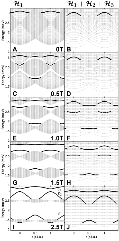
Figure 5: Eigenstates of the two-soliton Hamiltonian as a function of wavevector and energy at different fields, increasing from top to bottom. In each panel, states with the character of the $\varepsilon$ bound states have been highlighted in black. These states have been identified by being well separated from other states in energy, or, where they overlap with other states, by having high INS intensity and discarding regions with strong hybridization. Left column: Solution of $\mathcal{H}_{1}$. Three continua and three bound states can be seen at every non-zero field. $\varepsilon_{1}$, $\varepsilon_{2}$ and $\varepsilon_{-}$ are defined in Appendix D. Right column: solution of $\mathcal{H}=\mathcal{H}_{1}+\mathcal{H}_{2}+\mathcal{H}_{3}$. This comparison illustrates the key effect of $\mathcal{H}_{3}$, i.e., the presence of a longitudinal mean field: all continua are split into confinement bound states, but the $\varepsilon$ bound states are left essentially intact. This column is to be compared with the third column of Fig. 2, which shows the intensities under the same conditions.

In this Appendix, the two-soliton spectrum in various regimes is briefly discussed. The left column of Fig. 5 shows the two-soliton spectrum as a function of field for the minimal Hamiltonian $\mathcal{H}_{1}$. In this case, the spectrum consists of three continua and three bound states, whose origins are discussed in Sec. V, at every non-zero field. The right hand column of Fig. 5 shows the same calculation for the full Hamiltonian $\mathcal{H}_{1}+\mathcal{H}_{2}+\mathcal{H}_{3}$, where $\mathcal{H}_{3}$ is the confining mean field. In this case, the mean field splits the continua into a series of confinement bound states, but the $\varepsilon$ bound states are left mostly intact, because they are tightly bound.

Appendix D Bound state inversion and matrix elements of $\mathcal{H}_{2}$ in the localized limit

In this Appendix, we consider the spectrum near the localized limit, $h_{-}=0$, obtained when the transverse field satisfies $h_{y}=J\lambda_{yz}$. When $3J\lambda_{S}/(2\sqrt{2})>h_{+}$, as is the case for the experimentally relevant parameters, the top two $\varepsilon$ bound state modes cross each other, so we must use degenerate perturbation theory within the subspace of these top two modes to calculate the resulting spectrum.

The unperturbed bound states and their energies are given in (16). In the following, we consider the effects of various other terms in the Hamiltonian in (4) to (6), starting with the second term in $\mathcal{H}_{1}$. We consider the matrix elements between the two highest energy modes ($|\varepsilon_{+},k\rangle$ and $|\varepsilon_{0},k\rangle$) for the perturbation

$$V_{S}=\frac{-J\lambda_{S}}{2}\sum_{\text{sites},j}S_{j}^{+}S_{j+1}^{-}+S_{j}^{-}S_{j+1}^{+}.$$

This perturbation allows single spin flips to hop by one site. The diagonal matrix elements are

$$\langle\varepsilon_{+},k|V_{S}|\varepsilon_{+},k^{\prime}\rangle= \frac{-J\lambda_{S}}{4}(1+\cos kc)\,\delta_{k,k^{\prime}}$$

$$\langle\varepsilon_{0},k|V_{S}|\varepsilon_{0},k^{\prime}\rangle= \frac{+J\lambda_{S}}{2}(1+\cos kc)\,\delta_{k,k^{\prime}},$$

and are consistent with the expressions given in Sec. V. Within the degenerate subspace, off-diagonal matrix elements are

$$\langle\varepsilon_{0},k|V_{S}|\varepsilon_{+},k^{\prime}\rangle=\frac{iJ\lambda_{S}}{2\sqrt{2}}\sin(kc)\,\delta_{k,k^{\prime}}$$

and Hermitian conjugate. Eigenvalues and eigenvectors are then obtained by direct diagonalization, with the dynamical correlations $S^{xx}$ obtained from the eigenvectors as described in Sec. V.3. We term the resulting modes $\varepsilon_{1}$ and $\varepsilon_{2}$.

We also derive the matrix elements of the next nearest neighbour terms in $\mathcal{H}_{2}$. Consistent with the considerations above, we only keep the diagonal matrix elements between bound states of the same type, as well as the off-diagonal matrix elements between the middle and top modes $\varepsilon_{0}$ and $\varepsilon_{+}$, which show a strong mixing at the experimental parameters. The effect of the perturbation $V_{\text{AF}}$, (22), is to lower the energy of all states relative to the fully aligned (ground) state. However, as discussed in Appendix  B, this energy shift is different for states with a single spin flip compared to states with at least two spin flips, corresponding to two and four satisfied antiferromagnetic bonds, respectively. This leads to matrix elements

$$\langle\varepsilon_{+},k|V_{\text{AF}}|\varepsilon_{+},k^{\prime}\rangle=\langle\varepsilon_{-},k|V_{\text{AF}}|\varepsilon_{-},k^{\prime}\rangle= -\frac{3}{2}J\lambda_{\text{AF}}\delta_{k,k^{\prime}}$$

$$\langle\varepsilon_{0},k|V_{\text{AF}}|\varepsilon_{0},k^{\prime}\rangle= -J\lambda_{\text{AF}}\delta_{k,k^{\prime}}$$

$$\langle\varepsilon_{0},k|V_{\text{AF}}|\varepsilon_{+},k^{\prime}\rangle= \;0.$$

This perturbation also shifts the energies of all the continua by $-2J\lambda_{\text{AF}}$.

The effect of the perturbation $V_{\text{AF}}^{xy}$, (21), is to hop single spin flips by two sites. This leads to matrix elements

$$\langle\varepsilon_{+},k|V_{\text{AF}}^{xy}|\varepsilon_{+},k^{\prime}\rangle=\langle\varepsilon_{-},k|V_{\text{AF}}^{xy}|\varepsilon_{-},k^{\prime}\rangle= \frac{J\lambda_{\text{AF}}^{xy}}{2}\cos(kc)\delta_{k,k^{\prime}}$$

$$\langle\varepsilon_{0},k|V_{\text{AF}}^{xy}|\varepsilon_{0},k^{\prime}\rangle= J\lambda_{\text{AF}}^{xy}\cos(kc)\delta_{k,k^{\prime}}$$

$$\langle\varepsilon_{0},k|V_{\text{AF}}^{xy}|\varepsilon_{+},k^{\prime}\rangle= \;0.$$

To first order, this perturbation vanishes when acting on the continua. However, it mixes the continua with the bound states.

The interchain mean field term, $\mathcal{H}_{3}$, is

$$V_{z}=-h_{z}\sum_{\text{sites},j}S_{j}^{z}$$

under the approximation that $\langle\mathbf{S}\rangle=(0,0,1/2)$. The effect of this term on the bound states is determined by the matrix elements

$$\langle\varepsilon_{+},k|V_{z}|\varepsilon_{+},k^{\prime}\rangle=\langle\varepsilon_{-},k|V_{z}|\varepsilon_{-},k^{\prime}\rangle= \frac{3}{2}h_{z}\delta_{k,k^{\prime}}$$

$$\langle\varepsilon_{0},k|V_{z}|\varepsilon_{0},k^{\prime}\rangle= h_{z}\delta_{k,k^{\prime}}$$

$$\langle\varepsilon_{0},k|V_{z}|\varepsilon_{+},k^{\prime}\rangle= \;0.$$

The effect of this term on the continua is to confine the soliton pairs into a series of bound states; this effect cannot be captured within the current picture.

Finally we note that the first term in $\mathcal{H}_{2}$, $V_{A}$, (20), vanishes when projected to the subspace of bound states, since this term causes solitons to hop by two sites at a time. To understand the effect of this term on the continua, we note that $V_{A}$, a hopping term to a neighboring unit cell, shifts the single soliton dispersion relations as

$$\omega_{\pm}\longrightarrow\omega_{\pm}+J\lambda_{A}\cos(kc).$$

In contrast to the effect of the hopping $h_{-}$, $V_{A}$ induces the same shift in the energies of bonding / antibonding orbitals. As a result, this perturbation leads to the same energy change for the three continua,

$$\omega_{\sigma,\sigma^{\prime}} \longrightarrow\omega_{\sigma,\sigma^{\prime}}+J\lambda_{A}\left[\cos(k_{1}c)+\cos(k_{2}c)\right]$$

$$=\omega_{\sigma,\sigma^{\prime}}+J\lambda_{A}\cos\left(\dfrac{kc}{2}\right)\cos\left(\dfrac{qc}{2}\right),$$

for $\sigma,\sigma^{\prime}=\pm$, with total and relative momenta given by $k=k_{1}+k_{2}$ and $q=k_{1}-k_{2}$, respectively.

Alternatively, these spectra can be obtained by applying first order perturbation theory around the localized limit, similarly to the analysis of the hopping $h_{-}$ presented in the main text. To this end, we first evaluate the effect of $V_{A}$ on the states $|n,k\rangle$ constructed in Sec. V.2. We find

$${}^{\pm}\langle n^{\prime},k^{\prime}|V_{A}|n,k\rangle^{\pm}=^{0}_{\pm}\langle n^{\prime},k^{\prime}|V_{A}|n,k\rangle^{0}_{\pm}$$

$$\hskip 56.9055pt=J\lambda_{A}\cos\left(\frac{kc}{2}\right)\left(\delta_{n^{\prime},n+1}+\delta_{n^{\prime},n-1}\right)\delta_{k,k^{\prime}},$$

corresponding to an effective nearest neighbor hopping Hamiltonian for the relative coordinate $n$, with hopping amplitude $J\lambda_{A}\cos(kc/2)$, subject to the hard core constraint $n>0$. For the top and bottom continua, the hopping amplitude due to $V_{h_{-}}$ is also real, so the $|q,k\rangle^{\pm}$ states constructed in Sec. V.2 are also eigenstates of $V_{A}$ and the change in the energies is

$$\frac{{}^{\pm}\langle q,k|V_{A}|q,k\rangle^{\pm}}{{}^{\pm}\langle q,k|q,k\rangle^{\pm}}=2J\lambda_{A}\cos\left(\frac{kc}{2}\right)\cos\left(\frac{qc}{2}\right).$$

For the middle continuum, we consider the effect of ${V_{h_{-}}+V_{A}}$ on the plane wave

$$\sum_{n}e^{iqcn/2}(|n,k\rangle^{0}_{+}+|n,k\rangle^{0}_{-}).$$

We find that the perturbation corresponds to an effective nearest neighbour hopping Hamiltonian for the relative coordinate $n$, with complex hopping amplitude $t=J\lambda_{A}\cos(kc/2)+ih_{-}\sin(kc/2)=t^{\prime}+it^{\prime\prime}=|t|e^{i\varphi}$. This yields the dispersion

$$\omega^{A}_{+-}=J+2|t|\cos\left(\frac{qc}{2}+\varphi\right)$$

$$=J+2t^{\prime}\cos\left(\frac{qc}{2}\right)-2t^{\prime\prime}\sin\left(\frac{qc}{2}\right)=$$

$$J-2h_{-}\sin\left(\frac{kc}{2}\right)\sin\left(\frac{qc}{2}\right)+2J\lambda_{A}\cos\left(\frac{kc}{2}\right)\cos\left(\frac{qc}{2}\right).$$

The eigenstates satisfying the hard core repulsion boundary condition at $n=0$ can be obtained by noting that the plane wave with relative momentum $q$ is degenerate with the plane wave with relative momentum $-q-4\varphi/c$. Mixing these plane waves leads to the unnormalized eigenstates satisfying the hard core constraint,

$$\sum_{\begin{subarray}{c}\text{cell separation},\\ n>0\end{subarray}}\left(e^{iqcn/2}-e^{-i(qc/2+2\varphi)n}\right)\left(|n,k\rangle^{0}_{+}+|n,k\rangle^{0}_{-}\right).$$

For the plane wave

$$\sum_{n}e^{iqcn/2}(|n,k\rangle^{0}_{+}-|n,k\rangle^{0}_{-}),$$

the effect of $V_{h_{-}}+V_{A}$ corresponds to an effective nearest neighbour hopping Hamiltonian for the relative coordinate $n$, with complex hopping amplitude $t^{*}$, such that the argument above applies with $\varphi\rightarrow-\varphi$. Thus, the effect of the perturbation $V_{A}$ is to add $2J\lambda_{A}\cos(kc/2)\cos(qc/2)$ to the energies of all continua, as anticipated based on the single soliton dispersion relation. We also note that the argument above yields the following two degenerate eigenstates in the presence of $V_{h_{-}}$ but without $V_{A}$, i.e. for $\varphi=\pi/2$,

$$\sum_{n>0}\left(e^{icq_{\pm}n/2}-e^{-i(cq_{\pm}/2+\pi)n}\right)\left(|n,k\rangle^{0}_{+}\pm|n,k\rangle^{0}_{-}\right),$$

with $q_{+}-q_{-}=\pi$. The eigenstates constructed in the main text are the symmetric / antisymmetric combinations of these eigenstates.

For $\lambda_{A}<0$ and $h_{-}>0$ such as is found experimentally, the perturbation $V_{A}$ leads the top continuum to narrow and the bottom continuum to broaden, and the middle continuum to broaden around what would otherwise be the nodes. The plots in the right-most column of Fig. 2 include the effects of all terms in $\mathcal{H}_{1}$ and $\mathcal{H}_{2}$, but not $\mathcal{H}_{3}$ since it is not possible to include the effects of this last term on the continua in this framework.

References

- Sachdev [1999] S. Sachdev, Quantum Phase Transitions (Cambridge University Press, London, 1999).
- Pfeuty [1970] P. Pfeuty, The one-dimensional Ising model with a transverse field, Ann. Phys. (NY) 57, 79 (1970).
- Lieb et al. [1961] E. Lieb, T. Schultz, and D. Mattis, Two soluble models of an antiferromagnetic chain, Ann. Phys. (NY) 16, 407 (1961).
- McCoy and Wu [1978] B. M. McCoy and T. T. Wu, Two-dimensional Ising field theory in a magnetic field: Breakup of the cut in the two-point function, Phys. Rev. D 18, 1259 (1978).
- Coldea et al. [2010] R. Coldea, D. A. Tennant, E. M. Wheeler, E. Wawrzynska, D. Prabhakaran, M. Telling, K. Habicht, P. Smeibidl, and K. Kiefer, Quantum criticality in an Ising chain: Experimental evidence for emergent E8 symmetry, Science 327, 177 (2010).
- Kinross et al. [2014] A. W. Kinross, M. Fu, T. J. Munsie, H. A. Dabkowska, G. M. Luke, S. Sachdev, and T. Imai, Evolution of quantum fluctuations near the quantum critical point of the transverse field Ising chain system CoNb2O6, Phys. Rev. X 4, 031008 (2014).
- Morris et al. [2014] C. M. Morris, R. Valdés Aguilar, A. Ghosh, S. M. Koohpayeh, J. Krizan, R. J. Cava, O. Tchernyshyov, T. M. McQueen, and N. P. Armitage, Hierarchy of bound states in the one-dimensional ferromagnetic Ising chain CoNb2O6 investigated by high-resolution time-domain terahertz spectroscopy, Phys. Rev. Lett. 112, 137403 (2014).
- Liang et al. [2015] T. Liang, S. M. Koohpayeh, J. W. Krizan, T. M. McQueen, R. J. Cava, and N. P. Ong, Heat capacity peak at the quantum critical point of the transverse Ising magnet CoNb2O6, Nat. Commun. 6, 7611 (2015).
- Amelin et al. [2020] K. Amelin, J. Engelmayer, J. Viirok, U. Nagel, T. Rõõm, T. Lorenz, and Z. Wang, Experimental observation of quantum many-body excitations of E8 symmetry in the Ising chain ferromagnet CoNb2O6, Phys. Rev. B 102, 104431 (2020).
- Maartense et al. [1977] I. Maartense, I. Yaeger, and B. M. Wanklyn, Field-induced magnetic transitions of CoNb2O6 in ordered state, Solid State Commun. 21, 93 (1977).
- Scharf et al. [1979] W. Scharf, H. Weitzel, I. Yaeger, I. Maartense, and B. M. Wanklyn, Magnetic-structures of CoNb2O6, J. Magn. Magn. Mater. 13, 121 (1979).
- Mitsuda et al. [1994] S. Mitsuda, K. Hosoya, T. Wada, H. Yoshizawa, T. Hanawa, M. Ishikawa, K. Miyatani, K. Saito, and K. Kohn, Magnetic ordering in one-dimensional system CoNb2O6 with competing interchain interactions, J. Phys. Soc. Jpn. 63, 3568 (1994).
- Heid et al. [1995] C. Heid, H. Weitzel, P. Burlet, M. Bonnet, W. Gonschorek, T. Vogt, J. Norwig, and H. Fuess, Magnetic phase-diagram of CoNb2O6 - a neutron-diffraction study, J. Magn. Magn. Mater. 151, 123 (1995).
- Weitzel et al. [2000] H. Weitzel, H. Ehrenberg, C. Heid, H. Fuess, and P. Burlet, Lifshitz point in the three-dimensional magnetic phase diagram of CoNb2O6, Phys. Rev. B 62, 12146 (2000).
- Fava et al. [2020] M. Fava, R. Coldea, and S. A. Parameswaran, Glide symmetry breaking and Ising criticality in the quasi-1d magnet CoNb2O6, Proc. Natl. Acad. Sci. USA 117, 25219 (2020).
- Morris et al. [2021] C. M. Morris, N. Desai, J. Viirok, D. Hüvonen, U. Nagel, T. Rõõm, J. W. Krizan, R. J. Cava, T. M. McQueen, S. M. Koohpayeh, R. K. Kaul, and N. P. Armitage, Duality and domain wall dynamics in a twisted Kitaev chain, Nat. Phys. 17, 832 (2021).
- Woodland et al. [2023] L. Woodland, D. Macdougal, I. M. Cabrera, J. D. Thompson, D. Prabhakaran, R. I. Bewley, and R. Coldea, Tuning the confinement potential between spinons in the Ising chain compound CoNb2O6 using longitudinal fields and quantitative determination of the microscopic Hamiltonian, Phys. Rev. B 108, 184416 (2023).
- Prabhakaran et al. [2003] D. Prabhakaran, F. R. Wondre, and A. T. Boothroyd, Preparation of large single crystals of ANb2O6 (A=Ni, Co, Fe, Mn) by the floating-zone method, J. Cryst. Growth 250, 72 (2003).
- Wheeler [2007] E. M. Wheeler, Neutron scattering from low-dimensional quantum magnets, Ph.D. thesis, University of Oxford (2007).
- [20] Data archive weblink, http://dx.doi.org/10.5287/ora-braxw4ez1.