Generalized entropy for general subregions in
quantum gravity

Abstract

We consider quantum algebras of observables associated with subregions in theories of Einstein gravity coupled to matter in the $G_{N}\rightarrow 0$ limit. When the subregion is spatially compact or encompasses an asymptotic boundary, we argue that the algebra is a type II von Neumann factor. To do so in the former case we introduce a model of an observer living in the region; in the latter, the ADM Hamiltonian effectively serves as an observer. In both cases the entropy of states on which this algebra acts is UV finite, and we find that it agrees, up to a state-independent constant, with the generalized entropy. For spatially compact regions the algebra is type $\text{II}_{1}$, implying the existence of an entropy maximizing state, which realizes a version of Jacobson’s entanglement equilibrium hypothesis. The construction relies on the existence of well-motivated but conjectural states whose modular flow is geometric at an instant in time. Our results generalize the recent work of Chandrasekaran, Longo, Penington, and Witten on an algebra of operators for the static patch of de Sitter space.

Preprint MIT-CTP/5571

1 Introduction

A major lesson of modern physics is that it is fruitful to study entanglement measures in many-body quantum mechanical systems. These measures have many applications across physics, from quantum computing to the emergence of spacetime from conformal field theory. To discuss such measures in quantum mechanical systems, the usual starting point is a tensor product decomposition of the Hilbert space, from which one can obtain reduced density matrices. However, if one wishes to study entanglement measures in local quantum field theory by dividing the degrees of freedom according to where they live in space, there is an obstruction. While the Hilbert space of local quantum field theory has a tensor product decomposition in a lattice regularization, and thereby has reduced density matrices associated with a subregion, those reduced density matrices are ill-defined in the continuum limit. Said another way, subregions do not carry renormalized density matrices, but they do carry local operators and their algebras. Despite the absence of reduced density matrices, and correspondingly the absence of well-defined entanglement entropies, these local algebras possess relative entanglement measures such as mutual information and relative entropy  [1, 2].

In this work we are interested not in quantum field theory, but in quantum gravity coupled to matter in the $G_{N}\to 0$ limit. In this regime there is an effective field theory description at low energies [3, 4], where one can still divide space into subregions and associate local operators and thus their algebra with a region. Remarkably, coupling to gravity is expected to strengthen the tools of information theory by providing a renormalized notion of entanglement entropy for subregions given via the generalized entropy

$$S_{\text{gen}}=\left\langle\frac{A}{4\hbar G_{N}}\right\rangle+S_{\text{EE}},$$ (1.1)

consisting of a Bekenstein-Hawking-like term involving the area of the entangling surface and a term representing the entanglement entropy of the state of quantum fields restricted to the subregion. Each term in (1.1) is separately UV divergent—the second due to infinite vacuum entanglement in quantum field theory, the first due to loop effects that renormalize the gravitational coupling $G_{N}$—but a number of arguments suggest that these divergences cancel in their contributions to $S_{\text{gen}}$ in order to make it UV-finite and regulator-independent [5, 6, 7, 8, 9, 10]. This hints that $S_{\text{gen}}$ may represent the true entropy of the fundamental quantum gravitational degrees of freedom, which organizes into a sum of the two terms in (1.1) when working within the low energy effective theory.

This interpretation of $S_{\text{gen}}$ underlies many of the connections that have been discovered between quantum information and quantum gravity. These have their origin in black hole thermodynamics [11, 12], which first motivated the introduction of the generalized entropy in order to make sense of the second law of thermodynamics in the presence of black holes [13, 11]. The resulting generalized second law, which states that $S_{\text{gen}}$ increases under evolution to the future along the black hole horizon, provides a semiclassical upgrade of the classical area theorem of general relativity [14, 15]. This procedure of replacing areas with generalized entropies has been applied in several other contexts [16, 10, 17], leading to various semiclassical generalizations of classical theorems of general relativity, while at the same time providing information-theoretic explanations for why the theorems are true. Foremost among these is the quantum focusing conjecture [10], a semiclassical generalization of the classical focusing theorem that implies a number of other interesting statements about quantum field theory and semiclassical general relativity, such as the quantum null energy condition [10, 18, 19, 20] and the generalized second law for causal horizons [21, 22].

In holographic contexts, the generalized entropy features prominently in the Ryu-Takayanagi (RT) formula and its quantum generalizations [23, 24, 25, 26, 27]. The quantum-corrected formula states that the entanglement entropy of a subregion in the boundary conformal field theory is equal to the generalized entropy of a specific subregion in the dual bulk spacetime. The bulk subregion is selected by extremizing the generalized entropy over all choices of subregions in the bulk whose asymptotic boundary is the boundary subregion. The resulting bulk region is called an entanglement wedge, and its spatial boundary is known as a quantum extremal surface (QES). Considerations of entanglement entropies computed via the RT formula and quantum extremal surfaces have led to a wealth of ideas in holography and quantum gravity, including bulk reconstruction [28, 29, 30], connections between holography and quantum error correction [31, 32, 33, 34, 35, 36, 37], and the black hole information problem and the island formula [38, 39, 40, 41, 42, 43].

In fact, it has been shown that the semiclassical bulk dynamics are largely determined by demanding that the bulk geometry be consistent with the RT and QES formulas [44, 45, 46, 47, 48], allowing one to postulate that the bulk geometry arises entirely from the entanglement structure of the dual conformal field theory [49, 50]. The arguments leading to the derivation of bulk dynamics from the RT formula bear a close resemblance to previous works deriving the Einstein equation from horizon thermodynamics [51]. This connection is most explicit in Jacobson’s recent entanglement equilibrium conjecture, where the Einstein equation is argued to follow purely from bulk quantum gravity arguments and an assumption that the vacuum state restricted to a subregion has maximal entropy [52].

Given the wide range of applications and insights that rely on a notion of entanglement entropy for local subregions in quantum gravity, it is unsettling that such subregions are at the same time problematic. The culprit is diffeomorphism invariance, which tends to forbid the existence of localized gauge-invariant observables in both classical and quantum gravitational theories [53, 54, 55, 56]. The fact that diffeomorphisms can change the location of a subregion requires that the subregion be specified in an invariant manner; doing so leads to gravitational dressing of observables that can interfere with local algebraic properties such as microcausality [57, 58, 55, 56]. More generally, introducing a boundary gives rise to gravitational edge modes from diffeomorphisms acting near the boundary, leading to the concept of an extended phase space for quasilocal gravitational charges [59, 60, 61, 62, 63, 64, 65, 66, 67, 68, 69, 70].

Despite the challenges posed by diffeomorphism invariance, the numerous applications of generalized entropy detailed above suggest it should be well defined for generic subregions in semiclassical gravity [71]. Ideally it would arise as an entropy of a quasilocal operator algebra associated with the subregion, and this algebra would enable rigorous discussions of entanglement entropy and other quantum information theoretic quantities. A further desideratum of such an algebraic description is that it would make manifest the finiteness of the generalized entropy, demonstrating that the split into an area and entanglement entropy term as in (1.1) should simply be viewed as a choice of renormalization scheme. Doing so would bolster existing arguments in favor of finiteness of generalized entropy by providing an independent justification that does not rely on Euclidean methods, symmetry, or specific field content.

The goal of the present paper is to offer a proposal for such a quasilocal algebra of observables for subregions in semiclassical quantum gravity. This algebra is constructed in the limit of small gravitational coupling $G_{N}\rightarrow 0$, in which gravitational backreaction is suppressed. In this limit, the description in terms of quantum field theory in a fixed background is expected to capture the leading behavior, which can be further corrected order by order in the $G_{N}$ expansion. Since gravity can be treated as a low-energy effective field theory in this limit, one expects the language of local quantum field theory and von Neumann algebras [1, 72, 73] to be applicable in order to provide a description of the subregion algebras. In constructing such algebras, we will find that gravitational constraints arising from diffeomorphism invariance enter the description in a crucial way. Imposing these constraints results in an algebra in which entanglement entropy can be uniquely defined up to an overall additive ambiguity. Under regularization, this entropy agrees with generalized entropy up to the additive ambiguity, which can be thought of as a universal entanglement divergence.

Our construction of local gravitational algebras relies heavily on recent insights that have been made on strict large-$N$ limits in holography. These began with the works of Leutheusser and Liu [74, 75], which noted that the large $N$ limit of a holographic CFT above the Hawking-Page phase transition produces an emergent type $\text{III}_{1}$ von Neumann algebra, indicating the presence of a black hole horizon in the bulk gravitational theory. Type $\text{III}_{1}$ algebras are ubiquitous in quantum field theories when restricting to subregions [79, 80], and the emergent holographic algebra is naturally interpreted as the algebra of bulk quantum fields restricted to the black hole exterior. Subsequent work argued that generic causally complete subregions in the bulk theory should be associated with emergent type $\text{III}_{1}$ algebras in the boundary CFT [81, 82, 83]. An important further development was made by Witten, who demonstrated that the inclusion of $\frac{1}{N}$ corrections significantly changes the properties of the emergent algebras, resulting in algebras of type II [84]. Unlike their type III counterparts, type II von Neumann algebras possess well-defined notions of density matrices and traces [85, 86], and hence allow for renormalized entanglement entropies to be defined [87, 88, 89]. The renormalized entropy was then shown to agree, up to a state-independent constant, with the generalized entropy in the cases of the static patch of de Sitter space and the AdS black hole [90, 91]. Further investigations into algebraic constructions in JT gravity also yielded emergent type II algebras [92, 93], suggesting that such algebras appear generically in gravitational theories.

We will argue here that the same mechanism leading to type II algebras in the dS static patch and the AdS black hole applies to arbitrary subregions in quantum gravity. Thus, the appropriate algebraic formulation of gravitational subregions is in terms of type II von Neumann algebras. This represents a substantial generalization of the constructions presented in [84, 90, 91], which all involved symmetric configurations in which the subregion is bounded by a Killing horizon. Making the generalization to generic subregions requires two key modifications of the original arguments.

1. First, we will show that treating perturbative gravity carefully beyond linear order requires imposing gravitational constraints associated with subregion-preserving diffeomorphisms even when these diffeomorphisms are not isometries.

2. Second, we will argue that there are states on the subregion algebra whose modular flow generates boost-like diffeomorphisms in an infinitesimal neighborhood of a Cauchy slice, even when there is no global boost symmetry.

The details of our construction of a type II algebra for subregions in quantum gravity will closely follow the construction for the de Sitter static patch given by Chandrasekaran, Longo, Penington, and Witten (CLPW) in [90]. Most notably, this procedure involves the introduction of an observer degree of freedom within the subregion to serve as an anchor for gravitationally dressing operators in the subregion algebra. Rather than arguing for the existence of such an observer degree of freedom from first principles, we will show that introducing the observer has the desired effect of producing a local gravitational algebra in which the renormalized entropy agrees with the subregion generalized entropy. Additional arguments in favor of the existence of the observer come from considerations of the algebra for a region which extends out to infinity, discussed in section 5.5. In this case, the asymptotic boundary can be used as the observer, but since the resulting type II algebra must have a nontrivial commutant, we end up concluding that the local algebra associated with the causal complement must be associated with a type II algebra constructed with an observer degree of freedom. Further speculations on the nature of the observer are given in the discussion, section 6.4.

The final step in the construction of the algebra concerns energy conditions imposed on the observer. Just as in the CLPW construction, the observer can be restricted to have positive (or bounded below) energy, which is implemented via a projection in the crossed product algebra. For local gravitational subregions, this projection results in an algebra of type $\text{II}_{1}$, which, in particular, possesses a maximal entropy state. Intriguingly, the existence of a maximal entropy state for the gravitational subregion immediately implies a version of Jacobson’s entanglement equilibrium hypothesis [52]. When applied to the asymptotic boundary, the positive energy projection coincides with the positivity of the ADM energy, but due to certain sign differences, produces a type $\text{II}_{\infty}$ algebra, similar to the case of the AdS black hole [84, 91]. This suggests that bounded subregions in quantum gravity are associated with type $\text{II}_{1}$ algebras, while subregions that encompass an asymptotic boundary are type $\text{II}_{\infty}$. More succinctly, type II algebras arise for gravitational subregions with compact entangling surfaces.

The basic argument leading to the type II gravitational algebras is straightforward to state, and so we begin in section 2 with an overview of the argument. This section serves to clarify the logic of the paper and to emphasize the major results. The assumptions entering into the argument are then listed in section 2.1 to provide an easy reference for later discussions in the paper. A reader interested in understanding the main claims of this work is encouraged to read section 2 and then also section 6 which discusses numerous possible applications of the present work. The remaining sections provide further justifications and explanations of the assumptions listed in section 2.1 and describe in greater detail the properties of the type II gravitational algebras. Section 3 is devoted to describing the constraints appearing in gravity and their relation to diffeomorphism invariance. Following this, section 4 describes the relation between the boost diffeomorphism and modular flow, and gives evidence for the geometric modular flow conjecture. Section 5 gives details related to the type II gravitational algebras, leading to a demonstration that the algebraic entropy agrees with the subregion generalized entropy up to a state-independent constant. Several appendices are included that provide further details on gravitational constraints, von Neumann algebras, modular theory, and practical calculations within the crossed product algebra.

Note about related work: Shortly after this paper was first posted on the arXiv, two other papers appeared [94, 95] which have conceptual overlap with this one. We are also aware of forthcoming work by Kudler-Flam, Leutheusser, and Satishchandran [96] which realizes the crossed product explicitly for free fields on certain backgrounds, and of forthcoming work by Freidel and Gesteau [97] which discusses connections between crossed products and gravitational edge modes.

2 Outline of the construction

We begin with an overview of the general arguments leading to type II algebras for gravitational subregions and an associated calculation of generalized entropy, in order to clarify the major assumptions needed to reach the conclusion. The arguments will be based on purely bulk quantum gravitational considerations, in a low energy and weak gravitational coupling limit, $\varkappa\rightarrow 0$, with $\varkappa=\sqrt{32\pi G_{N}}$.

Free graviton theory

The first step is to consider the theory of Einstein gravity minimally coupled to matter in the strict $\varkappa\rightarrow 0$ limit. This limit suppresses gravitational backreaction, and hence is described in terms of quantum fields propagating on a background with a fixed metric $g_{ab}^{0}$ which we will take to be globally hyperbolic. Treating gravity as an effective field theory, the gravitons can be quantized in a similar manner to the ordinary matter fields. This is done by expanding the metric around the background according to

$$g_{ab}=g_{ab}^{0}+\varkappa h_{ab},$$ (2.1)

and quantizing the metric perturbation $h_{ab}$ as a free, massless, spin-2 field. The coefficient of $h_{ab}$ is chosen to give it a canonical normalization in the quadratic action, and this also suppresses graviton interactions in the $\varkappa\rightarrow 0$ limit.

Diffeomorphisms that preserve the decomposition (2.1) are generated by vector fields $\varkappa\xi^{a}$ proportional to $\varkappa,$ which act trivially on matter fields in the $\varkappa\to 0$ limit while generating an abelian algebra of linearized gauge transformations for the graviton, $\delta_{\varkappa\xi}h_{ab}=\pounds_{\xi}g_{ab}^{0}.$ Because the action of diffeomorphisms is suppressed in $\varkappa$, there is no issue in defining arbitrary subregions in the background geometry and analyzing the algebra of matter fields and free gravitons restricted to these subregions. We will fix a subregion $\mathcal{S}$ by choosing it to coincide with the domain of dependence $D(\Sigma)$ of a partial Cauchy slice $\Sigma$ with boundary $\tilde{\partial}\Sigma$, where the $\tilde{\partial}$ notation refers to the finite-distance boundary of $\Sigma$, and excludes any asymptotic boundaries (see figure 1). We will use the symbol $\bar{\Sigma}$ to denote a complementary partial Cauchy slice, also with boundary $\tilde{\partial}\bar{\Sigma}=\tilde{\partial}\Sigma,$ so that $\Sigma_{c}=\Sigma\cup\bar{\Sigma}$ is a Cauchy slice for the spacetime. According to general arguments from algebraic quantum field theory [79, 80], the algebra $\mathcal{A}_{\text{QFT}}$ associated with $\mathcal{S}$ is a von Neumann factor of type $\text{III}_{1}$ for any quantum field theory with a UV fixed point. This algebra is realized as a collection of bounded operators acting on a Hilbert space $\mathcal{H}_{\text{QFT}}$. By assuming Haag duality [98, 1], the algebra of quantum fields for the complementary domain of dependence $\mathcal{S}^{\prime}=D(\bar{\Sigma})$ can be taken to coincide with the commutant algebra $\mathcal{A}_{\text{QFT}}^{\prime}$ consisting of all bounded operators acting on $\mathcal{H}_{\text{QFT}}$ that commute with $\mathcal{A}_{\text{QFT}}$. This commutant algebra is also type $\text{III}_{1}$.

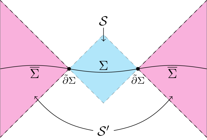
(a)

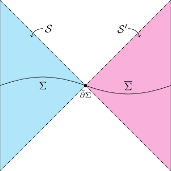
(b)

Figure 1: Two examples of a partial Cauchy slice $\Sigma,$ its causal development $\mathcal{S}$, the complementary region $\mathcal{S}^{\prime},$ and the entangling surface $\partial\Sigma.$ In example (1(a)), $\mathcal{S}$ is bounded while $\mathcal{S}^{\prime}$ is unbounded, while in example (1(b)), both $\mathcal{S}$ and $\mathcal{S}^{\prime}$ are unbounded.

The subregion $\mathcal{S}$ can either be bounded, by which we mean that it has a bounded Cauchy surface $\Sigma$, as in figure 1(1(a)), or unbounded, meaning it contains a complete asymptotic boundary, as in figure 1(1(b)). The constructions we are about to describe for of the gravitational algebras in each case are similar, with the main qualitative difference being that bounded regions will result in type $\text{II}_{1}$ algebras while unbounded regions will result in type $\text{II}_{\infty}$ algebras. Since the algebra of the causal complement $\mathcal{S}^{\prime}$ naturally arises as the commutant of the subregion algebra, both cases can be handled at once if $\mathcal{S}$ is chosen to be a bounded subregion in an open universe, so that $\mathcal{S}^{\prime}$ is unbounded. We therefore restrict attention to this case for the remainder of this section. Since $\Sigma$ then has no asymptotic boundaries, we will simply write $\partial\Sigma$ for $\tilde{\partial}\Sigma$.

Gravitational interactions and constraints

The next step is to consider corrections coming from the $\varkappa$ expansion. A significant change is that at first interacting order in $\varkappa$, all matter fields $\phi$ transform under rescaled diffeomorphisms, $\delta_{\xi}\phi=\varkappa\pounds_{\xi}\phi$. The transformation of the graviton is similar, $\delta_{\xi}h_{ab}=\varkappa\pounds_{\xi}h_{ab}+\pounds_{\xi}g^{0}_{ab}$, with the first term representing the diffeomorphism transformation of the spin-2 field $h_{ab}$, and the second term still interpreted as a linearized gauge transformation. Because of these nontrivial transformations, care has to be taken in order to ensure that the algebra we construct is diffeomorphism-invariant. It is useful to break this problem into two parts: first, ensuring that the algebra is invariant under diffeomorphisms that are supported locally within the subregion $\mathcal{S}$, and then ensuring invariance under the wider class of diffeomorphisms that act simultaneously on $\mathcal{S}$ and $\mathcal{S}^{\prime}$.

Diffeomorphism invariance within $\mathcal{S}$ can be addressed either by gravitationally dressing operators within the subregion, or by partially fixing the gauge to set up a well-defined coordinate system within $\mathcal{S}$. The local gravitational dressing can be constructed perturbatively in the $\varkappa$ expansion [58, 56], and it is generally expected that the algebra $\mathcal{A}_{\text{QFT}}$ remains type $\text{III}_{1}$ upon including these perturbative corrections [74, 75, 84]. Operators in $\mathcal{A}_{\text{QFT}}^{\prime}$ must similarly be gravitationally dressed, and it is important to choose this dressing to ensure that $\mathcal{A}_{\text{QFT}}$ and $\mathcal{A}_{\text{QFT}}^{\prime}$ remain commutants of each other. A straightforward way to enforce this requirement is to dress both sets of operators to the entangling surface $\partial\Sigma$ which is held fixed (see, e.g. [99]); doing so should prevent the gravitational dressings for the different subregions from overlapping, thus preserving microcausality.

Because such dressings are necessarily quasilocal, there remain additional conditions from requiring invariance under diffeomorphisms that act in both $\mathcal{S}$ and $\mathcal{S}^{\prime}$. Of particular importance are diffeomorphisms that generate boosts around the entangling surface, as in figure 2. These diffeomorphisms are generated by vector fields $\xi^{a}$ that are future-directed in $\mathcal{S}$, past-directed in $\mathcal{S}^{\prime}$, and tangent to the null boundaries of the subregions so that they map $\mathcal{S}$ and $\mathcal{S}^{\prime}$ into themselves. Furthermore, $\xi^{a}$ must vanish at the entangling surface $\partial\Sigma$ and have constant surface gravity $\kappa$ on $\partial\Sigma$, defined by the relation

$$\nabla_{a}\xi_{b}\overset{\partial\Sigma}{=}\kappa n_{ab},$$ (2.2)

where $n_{ab}$ is the unit binormal to $\partial\Sigma$, i.e., the unique antisymmetric tensor that is normal to $\partial\Sigma$, co-oriented with the normal bundle of $\partial\Sigma$, and satisfies $n^{ab}n_{ab}=-2$.

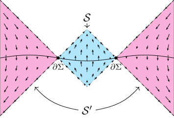
Figure 2: A vector field $\xi^{a}$ that is future-directed in $\mathcal{S},$ past-directed in $\mathcal{S}^{\prime},$ tangent to the null boundaries, and approximates a boost near the entangling surface $\partial\Sigma.$

We will choose one such diffeomorphism and study the effects of imposing it as a constraint on the algebras $\mathcal{A}_{\text{QFT}}$ and $\mathcal{A}_{\text{QFT}}^{\prime}.$ This can be done by writing an expression for the associated constraint functional in the full nonlinear theory of gravity, and imposing that constraint on $\mathcal{A}_{\text{QFT}}$ and $\mathcal{A}_{\text{QFT}}^{\prime}$ order by order in $\varkappa$. However, just as in the CLPW construction [90], it is problematic to impose this constraint solely on the quantum field degrees of freedom comprising $\mathcal{A}_{\text{QFT}}$ and $\mathcal{A}_{\text{QFT}}^{\prime}$. Instead, we introduce an observer degree of freedom into the subregion $\mathcal{S}$ by tensoring in an additional Hilbert space $\mathcal{H}_{\text{obs}}=L^{2}(\mathbb{R})$. This observer is used both to define location of the subregion beyond leading order in $\varkappa$ and to serve as a clock providing a physical notion of time evolution for quantum fields within $\mathcal{S}$. It is not necessary to view the observer as a literal particle following a worldline within the subregion, and, as discussed in section 5.5, the construction of the gravitational subregion algebra is largely agnostic to the details of the observer model. The main requirement is that the observer couple universally to gravity via its energy-momentum, which implies that the observer Hamiltonian must appear in the gravitational constraints. Following CLPW [90], we take the observer’s Hamiltonian to be the position operator $H_{\text{obs}}=\hat{q}$, in which case the conjugate momentum $\hat{p}=-i\frac{d}{dq}$ has the interpretation of the time measured by the observer. The full observer algebra is taken to be the set of all bounded operators acting on $\mathcal{H}_{\text{obs}}$, $\mathcal{A}_{\text{obs}}=\mathcal{B}(\mathcal{H}_{\text{obs}})$. The complementary region $\mathcal{S}^{\prime}$ must also have an observer degree of freedom, but because $\mathcal{S}^{\prime}$ contains an asymptotic boundary, the role of the observer is played by the ADM Hamiltonian $H_{\text{ADM}}$. It acts on a separate Hilbert space $\mathcal{H}_{\text{ADM}}$, and the full asymptotic observer algebra includes all bounded operators on this Hilbert space, $\mathcal{A}_{\text{ADM}}=\mathcal{B}(\mathcal{H}_{\text{ADM}})$.

Together, the full kinematical algebra is $(\mathcal{A}_{\text{QFT}}\vee\mathcal{A}_{\text{QFT}}^{\prime})\otimes\mathcal{A}_{\text{obs}}\otimes\mathcal{A}_{\text{ADM}}$, which acts on the Hilbert space $\mathcal{H}_{\text{kin}}=\mathcal{H}_{\text{QFT}}\otimes\mathcal{H}_{\text{obs}}\otimes\mathcal{H}_{\text{ADM}}$. The tensor product structure reflects the fact that $\mathcal{A}_{\text{obs}}$ and $\mathcal{A}_{\text{ADM}}$ commute with the quantum field degrees of freedom before imposing the gravitational constraint. As explained in section 3, the constraint is given by

$$\mathcal{C}[\xi]=H_{\xi}^{g}+H_{\text{obs}}+H_{\text{ADM}},$$ (2.3)

where $H_{\xi}^{g}$ is the operator generating the flow of $\xi^{a}$ on the quantum field algebras $\mathcal{A}_{\text{QFT}}$ and $\mathcal{A}_{\text{QFT}}^{\prime}$ instantaneously on $\Sigma_{c}$. It takes the form of a local integral of the matter and graviton stress tensors, as explained in section 3.2.

Crossed product algebra

To implement the constraint at the level of the subregion algebra, we need to determine the operators in $\mathcal{A}_{\text{QFT}}\otimes\mathcal{A}_{\text{obs}}$ that commute with $\mathcal{C}[\xi]$. Because both algebras already commute with $H_{\text{ADM}}$, the desired subalgebra consists of all operators commuting with the flow of $\mathcal{C}=H_{\xi}^{g}+H_{\text{obs}}=H_{\xi}^{g}+\hat{q}$. This can alternatively be characterized as the set of operators on $\mathcal{H}_{\text{QFT}}\otimes\mathcal{H}_{\text{obs}}$ commuting with $\mathcal{C}$ as well as $\mathcal{A}_{\text{QFT}}^{\prime}$. As explained in appendix B, the resulting von Neumann algebra is the crossed product of $\mathcal{A}_{\text{QFT}}$ by the flow generated by $H_{\xi}^{g}.$ It is generated by elements of the form $e^{iH_{\xi}^{g}\hat{p}}\mathsf{a}e^{-iH_{\xi}^{g}\hat{p}}$ with $\mathsf{a}\in\mathcal{A}_{\text{QFT}}$, along with $e^{i\hat{q}t}$ for $t\in\mathbb{R}$; in other words, the gauge-invariant algebra for the subregion $\mathcal{S}$ is given by

$$\mathcal{A}^{\mathcal{C}}=\{e^{iH_{\xi}^{g}\hat{p}}\mathsf{a}e^{-iH_{\xi}^{g}\hat{p}},e^{i\hat{q}t}\,|\,\mathsf{a}\in\mathcal{A}_{\text{QFT}},t\in\mathbb{R}\}^{\prime\prime},$$ (2.4)

where $S^{\prime\prime}$ denotes the smallest von Neumann algebra containing the set $S$. We can think of the operators $e^{i\hat{q}t}$ as generating the algebra of operators that are diagonal in the observer energy basis, and the operators $e^{iH_{\xi}^{g}\hat{p}}\mathsf{a}e^{-iH_{\xi}^{g}\hat{p}}$ as being dressed versions of operators in $\mathcal{A}_{\text{QFT}}$ where the observer clock has been synchronized with the time experienced by field-theoretic degrees of freedom.

Properly implementing the constraints at the level of the Hilbert space effectively eliminates the factor of $\mathcal{H}_{\text{ADM}}$ from $\mathcal{H}_{\text{kin}}$ (see section 5.1 and [90]), leading to the representation of $\mathcal{A}^{\mathcal{C}}$ acting on $\mathcal{H}_{\text{QFT}}\otimes\mathcal{H}_{\text{obs}}$ described above. In this description, the ADM Hamiltonian is represented by $H_{\text{ADM}}=-\mathcal{C}=-H_{\xi}^{g}-\hat{q}$. By construction, this operator, along with $\mathcal{A}_{\text{QFT}}^{\prime}$, generates the commutant algebra,

$$(\mathcal{A}^{\mathcal{C}})^{\prime}=\{\mathsf{b}^{\prime},e^{i(H_{\xi}^{g}+\hat{q})s}|\mathsf{b}^{\prime}\in\mathcal{A}_{\text{QFT}}^{\prime},s\in\mathbb{R}\}^{\prime\prime},$$ (2.5)

and this is naturally identified as the algebra associated with the complementary subregion $\mathcal{S}^{\prime}$. This algebra is an equivalent representation of the crossed product of $\mathcal{A}_{\text{QFT}}^{\prime}$ by the flow generated by $H_{\xi}^{g}$.

Geometric modular flow

Having obtained the subregion algebra $\mathcal{A}^{\mathcal{C}}$ as a crossed product with respect to the flow generated by $H_{\xi}^{g}$, the next task is to determine the type of the resulting von Neumann algebra. Our claim is that this algebra is type $\text{II}_{\infty}$, and coincides with the crossed product of $\mathcal{A}_{\text{QFT}}$ with respect to a modular automorphism group, in direct analogy with previous examples for subregions with boost symmetry [84, 90, 91].

This claim relies on a conjecture that $H_{\xi}^{g}$ is in fact proportional to the modular Hamiltonian for some state on the algebra $\mathcal{A}_{\text{QFT}}$. The intuitive argument for this conjecture is that any flow that agrees with the vacuum modular flow in the UV (i.e., on degrees of freedom localized close to the entangling surface) should define a valid modular flow for some state on the algebra. Since any entangling surface looks locally like Rindler space at short enough distances, we need only require that the flow generated by $H_{\xi}^{g}$ agree near the entangling surface with the vacuum modular flow for this local Rindler space. As is well known from the work of Bisognano and Wichmann [100], the vacuum modular flow of Rindler space is simply the geometric flow of a boost that fixes the entangling surface. Hence, by choosing $\xi^{a}$ to look like a boost with constant surface gravity near $\partial\Sigma$, we conjecture this ensures that $H_{\xi}^{g}$ generates a modular flow of some state $|\Psi\rangle\in\mathcal{H}_{\text{QFT}}$. The surface gravity determines the constant of proportionality between $H_{\xi}^{g}$ and $h_{\Psi}$,

$$h_{\Psi}=\beta H_{\xi}^{g}=\frac{2\pi}{\kappa}H_{\xi}^{g},$$ (2.6)

as follows from the Unruh effect [101] associated with the local Rindler space near the entangling surface. Equivalently, this relation implies that $|\Psi\rangle$ satisfies the KMS condition at inverse temperature $\beta=\frac{2\pi}{\kappa}$ for the flow generated by $H_{\xi}^{g}$. Additional arguments in favor of this geometric modular flow conjecture are presented in section 4.

Note that when $\xi^{a}$ does not generate a symmetry of the background metric, the Hamiltonian generating the flow of $\xi^{a}$ will be time-dependent. This means that the time-independent operator $H_{\xi}^{g}$ only generates this flow instantaneously on the initial Cauchy surface $\Sigma_{c}$, and hence the modular flow looks local only in the vicinity of $\Sigma_{c}$. Fortunately, this is all that is needed to identify the modular crossed product algebra with the gauge-invariant gravitational algebra. Due to time dependence, the Hamiltonian constructed on a different Cauchy slice will differ from $H_{\xi}^{g}$, and therefore define a different KMS state. This will result in an isomorphic crossed-product algebra whose states and operators are simply related to those of $\mathcal{A}^{\mathcal{C}}$.

Modular operators and density matrices

In addition to supporting the conclusion that $\mathcal{A}^{\mathcal{C}}$ is a type $\text{II}_{\infty}$ von Neumann algebra, the assumption that $\beta H_{\xi}^{g}$ is a modular Hamiltonian of some state on $\mathcal{A}_{\text{QFT}}$ allows one to leverage the full machinery of modular theory (reviewed in appendix C) in order to compute density matrices and entropies in $\mathcal{A}^{\mathcal{C}}$. The existence of well-defined density matrices, along with the related existence of a renormalized trace, are key features of type II von Neumann factors, and both are uniquely determined up to a state-independent multiplicative constant. These properties follow from the fact that the modular operator $\Delta_{\widehat{\Phi}}$ associated to $\mathcal{A}^{\mathcal{C}}$ for any state $|\widehat{\Phi}\rangle\in\mathcal{H}_{\text{QFT}}\otimes\mathcal{H}_{\text{obs}}$ factorizes into separate operators respectively affiliated with $\mathcal{A}^{\mathcal{C}}$ and $(\mathcal{A}^{\mathcal{C}})^{\prime}$ according to

$$\Delta_{\widehat{\Phi}}=\rho_{\widehat{\Phi}}(\rho_{\widehat{\Phi}}^{\prime})^{-1}.$$ (2.7)

The factors in this relation determine the density matrix $\rho_{\widehat{\Phi}}$ for $\mathcal{A}^{\mathcal{C}}$ and the density matrix $\rho_{\widehat{\Phi}}^{\prime}$ for $(\mathcal{A}^{\mathcal{C}})^{\prime}$.

As a concrete demonstration of this factorization, we consider a class of states of the form $|\widehat{\Phi}\rangle=|\Phi\rangle\otimes|f\rangle$ where $|\Phi\rangle\in\mathcal{H}_{\text{QFT}}$ and $|f\rangle=f(q)$ is a wavefunction in $\mathcal{H}_{\text{obs}}$. The factors of the modular operator can be determined exactly (see section 5.2 and appendix E), resulting in the density matrices

$$\rho_{\widehat{\Phi}} =\frac{1}{\beta}e^{i\hat{p}\frac{h_{\Psi}}{\beta}}f\Big{(}\hat{q}-\frac{h_{\Psi}}{\beta}\Big{)}e^{\frac{\beta\hat{q}}{2}}\Delta_{\Phi|\Psi}e^{\frac{\beta\hat{q}}{2}}f^{*}\Big{(}\hat{q}-\frac{h_{\Psi}}{\beta}\Big{)}e^{-i\hat{p}\frac{h_{\Psi}}{\beta}}$$ (2.8)

$$\rho_{\widehat{\Phi}}^{\prime} =\frac{1}{\beta}\Delta_{\Psi|\Phi}^{-\frac{1}{2}}J_{\Phi|\Psi}J_{\Psi}e^{\frac{\beta\hat{q}}{2}}\,\Big{|}f\Big{(}\hat{q}+\frac{h_{\Psi}}{\beta}\Big{)}\Big{|}^{2}e^{\frac{\beta\hat{q}}{2}}J_{\Psi}J_{\Psi|\Phi}\Delta_{\Psi|\Phi}^{-\frac{1}{2}},$$ (2.9)

where the relative modular operators $\Delta_{\Phi|\Psi}$, $\Delta_{\Psi|\Phi}$ and modular conjugations $J_{\Psi}$, $J_{\Psi|\Phi}$, $J_{\Phi|\Psi}$ are defined in appendix C.

Generalized entropy

With the expression for $\rho_{\widehat{\Phi}}$ in hand, the entropy can be computed as the expectation value of $-\log\rho_{\widehat{\Phi}}$,

$$S(\rho_{\widehat{\Phi}})=\langle\widehat{\Phi}|-\log\rho_{\widehat{\Phi}}|\widehat{\Phi}\rangle.$$ (2.10)

In order to simplify the computation of the logarithm, we impose the same semiclassical assumption on the observer wavefunction $f(q)$ as employed in [90, 91], namely that it is slowly varying. This amounts to assuming that the entanglement between the observer and the quantum field degrees of freedom is negligible, and allows us to ignore commutators of the form $[f\left(\hat{q}-\frac{h_{\Psi}}{\beta}\right),\Delta_{\Phi|\Psi}]$ appearing in $\log\rho_{\widehat{\Phi}}$. Under this assumption, the entropy can be expressed as (see section 5)

$$S(\rho_{\widehat{\Phi}})=-S_{\text{rel}}(\Phi||\Psi)-\beta\langle H_{\text{obs}}\rangle_{f}+S_{f}^{\text{obs}}+\log\beta,$$ (2.11)

where $S_{\text{rel}}(\Phi||\Psi)$ is the relative entropy between the states $|\Phi\rangle$ and $|\Psi\rangle$ in the algebra $\mathcal{A}_{\text{QFT}}$, and $S_{f}^{\text{obs}}$ is the entropy associated with the probability distribution derived from the observer’s wavefunction. This expression for the entropy is manifestly UV finite for a wide class of states and hence defines a good notion of renormalized entropy for the subregion. This formula for the entropy is closely related to expressions from [90, 91] applicable to subregions possessing boost symmetry. Note that the multiplicative ambiguity in the definition of $\rho_{\widehat{\Phi}}$ translates to a state-independent additive ambiguity in $S(\rho_{\widehat{\Phi}})$, reflected in the constant $\log\beta$ term in (2.11). This ambiguity is discussed in more detail in sections 5.2 and 5.3.

We can also relate $S(\rho_{\widehat{\Phi}})$ to the generalized entropy for the subregion. Because $|\Psi\rangle$ is a KMS state for $H_{\xi}^{g}$, the relative entropy in (2.11) can be expressed as a free energy with respect to the one-sided Hamiltonian for the subregion $H^{\Sigma}_{\xi}$,

$$S_{\text{rel}}(\Phi||\Psi)=\beta\langle H_{\xi}^{\Sigma}\rangle_{\Phi}-S_{\Phi}^{\text{mat}}+\text{const.},$$ (2.12)

with the constant state-independent. Each term in this expression is separately UV divergent, but the combination is finite for states with finite relative entropy with respect to $|\Psi\rangle$. To convert this to a generalized entropy, we note that when the local gravitational constraints are satisfied on the subregion Cauchy surface $\Sigma$, the total energy in the subregion is related to the bounding area according to (see section 3.1)

$$H_{\xi}^{\Sigma}+H_{\text{obs}}=-\frac{\kappa}{2\pi}\frac{A}{4G_{N}}.$$ (2.13)

This relation is the integrated form of the first law of local subregions, an analog of the first law of black hole mechanics that is applicable to generic subregions in gravitational theories. Applying these relations to (2.11), we arrive at the result

$$S(\rho_{\widehat{\Phi}})=\left\langle\frac{A}{4G_{N}}\right\rangle_{\widehat{\Phi}}+S^{\text{mat}}_{\Phi}+S_{f}^{\text{obs}}+\text{const.}=S_{\text{gen}}+\text{const.},$$ (2.14)

demonstrating that the algebraic entropy $S(\rho_{\widehat{\Phi}})$ computed in $\mathcal{A}^{\mathcal{C}}$ agrees with the subregion generalized entropy up to a state-independent constant. Note that invoking the local first law of subregions simplifies the derivation of the generalized entropy from (2.11) relative to the original arguments appearing in [90, 91].

Type $\text{II}_{1}$/Type $\text{II}_{\infty}$ algebras from energy conditions

We next turn to the question of energy conditions satisfied by the observer. Although we do not at present have a detailed model for the observer, a reasonable requirement to avoid instabilities is that the observer energy be bounded below, as was assumed by CLPW in [90]. This can be implemented by acting with a step function projection $\Pi_{\text{o}}=\Theta(H_{\text{obs}})=\Theta(\hat{q})$, on all elements of $\mathcal{A}^{\mathcal{C}}$. The resulting algebra $\widetilde{\mathcal{A}}=\Pi_{\text{o}}\mathcal{A}^{\mathcal{C}}\Pi_{\text{o}}$ consists of all operators of the form $\Pi_{\text{o}}\,\widehat{\mathsf{a}}\,\Pi_{\text{o}}$, with $\widehat{\mathsf{a}}\in\mathcal{A}^{\mathcal{C}}$. As explained in section 5.4 and appendix B, the effect of this projection on the algebra can be diagnosed by evaluating the trace of $\Pi_{\text{o}}$ in $\mathcal{A}^{\mathcal{C}}$. This trace is defined on $\widehat{\mathsf{a}}\in\mathcal{A}^{\mathcal{C}}$ by

$$\widehat{\operatorname{Tr}}\;\widehat{\mathsf{a}}=2\pi\beta\langle\Psi|\langle 0|_{p}e^{-\frac{\beta\hat{q}}{2}}\,\widehat{\mathsf{a}}\,e^{-\frac{\beta\hat{q}}{2}}|0\rangle_{p}|\Psi\rangle,$$ (2.15)

where $|0\rangle_{p}$ is the zero momentum eigenstate. $\widehat{\operatorname{Tr}}$ can be viewed as a renormalized version of the standard Hilbert space trace that preserves cyclicity $\widehat{\operatorname{Tr}}(\widehat{\mathsf{a}}\,\widehat{\mathsf{b}})=\widehat{\operatorname{Tr}}(\widehat{\mathsf{b}}\,\widehat{\mathsf{a}})$ and satisfies good physical properties including faithfulness, semifiniteness, and normality. See section 5.2 and appendix B for further discussion of this trace.

From this definition, the trace of $\Pi_{\text{o}}$ is readily evaluated,

$$\widehat{\operatorname{Tr}}(\Pi_{\text{o}})=\beta\int_{0}^{\infty}dye^{-\beta y}=1.$$ (2.16)

Because $\widehat{\operatorname{Tr}}(\Pi_{\text{o}})$ is finite, the projected algebra $\widetilde{\mathcal{A}}$ is a factor of type $\text{II}_{1}$. This matches the algebra type obtained by CLPW for the static patch of de Sitter space. Type $\text{II}_{1}$ algebras have the property of possessing a maximum entropy state whose density matrix coincides with the identity operator. This state is given by

$$|\Psi_{\text{max}}\rangle=|\Psi,\sqrt{\beta}e^{-\frac{\beta q}{2}}\Theta(q)\rangle.$$ (2.17)

The existence of such a maximal entropy state immediately implies a version of Jacobson’s entanglement equilibrium hypothesis [52], which conjectured that the entropy of the vacuum for small causal diamonds is maximal in quantum gravity theories. Given the form of the maximal entropy state (2.17), we see that it is the KMS state $|\Psi\rangle$ that defines the maximal entropy state, which reduces to the vacuum state only for special choices of subregions and matter content.

The energy conditions for the complementary region $\mathcal{S}^{\prime}$ can also be analyzed from the perspective of the commutant algebra $(\mathcal{A}^{\mathcal{C}})^{\prime}$. As discussed in section 5.5, the ADM Hamiltonian is represented on $\mathcal{H}_{\text{QFT}}\otimes\mathcal{H}_{\text{obs}}$ by the operator $-H_{\xi}^{g}-\hat{q}$, and hence the projection to positive ADM energy is implemented by $\Pi_{\text{ADM}}=\Theta\left(-\frac{h_{\Psi}}{\beta}-\hat{q}\right)\in(\mathcal{A}^{\mathcal{C}})^{\prime}$. Equation (2.15) also defines a trace on $(\mathcal{A}^{\mathcal{C}})^{\prime}$, and on $\Pi_{\text{ADM}}$ this trace is infinite,

$$\widehat{\operatorname{Tr}}(\Pi_{\text{ADM}})=\infty.$$ (2.18)

Accordingly, the projected algebra $\Pi_{\text{ADM}}(\mathcal{A}^{\mathcal{C}})^{\prime}\Pi_{\text{ADM}}$ remains type $\text{II}_{\infty}$. This reflects a generic feature of unbounded subregion algebras: the projection to positive ADM energy is always infinite for such gravitational algebras due to the way the ADM Hamiltonian appears in the gravitational constraint. The resulting picture is that bounded subregions are associated with type $\text{II}_{1}$ algebras possessing maximal entropy states, while unbounded subregions produce type $\text{II}_{\infty}$ algebras and correspondingly have no maximal entropy state.

2.1 List of assumptions

The construction outlined above provides evidence that local subregions in gravity should be associated with type II von Neumann algebras, and that doing so leads to an algebraic interpretation of the generalized entropy. This conclusion relies on a number of assumptions, which we list here in order to clarify the logic of the argument. In much of the remainder of the paper, we discuss these assumptions in greater detail and give partial evidence for them.

Assumptions:

1. There exist algebras $\mathcal{A}_{\text{QFT}}$, $\mathcal{A}_{\text{QFT}}^{\prime}$ (which we call “kinematical”) describing the quantum field degrees of freedom (including linearized gravitons) associated with the causally complementary subregions $\mathcal{S}$ and $\mathcal{S}^{\prime}$. These algebras are perturbatively definable order by order in the $\varkappa$ expansion, and remain type $\text{III}_{1}$ and commutants of each other to all orders in $\varkappa$.

2. There exist auxiliary observer degrees of freedom associated with the subregions $\mathcal{S}$ and $\mathcal{S}^{\prime}$ described by type $\text{I}_{\infty}$ algebras $\mathcal{A}_{\text{obs}},\mathcal{A}_{\text{obs}}^{\prime}$ that commute with $\mathcal{A}_{\text{QFT}}$ and $\mathcal{A}_{\text{QFT}}^{\prime}$ to all orders in $\varkappa$.

3. The physical gravitational algebra arises from imposing the constraint $\mathcal{C}[\xi]=H_{\xi}^{g}+H_{\text{observers}}$, where $H_{\xi}^{g}$ is the generator of a specific boost-like flow on $\mathcal{A}_{\text{QFT}}$ and $\mathcal{A}_{\text{QFT}}^{\prime}$, and $H_{\text{observers}}$ refers to the Hamiltonian of the auxiliary observer degrees of freedom associated with $\mathcal{S}$ and $\mathcal{S}^{\prime}$.

4. The flow generated by $H_{\xi}^{g}$ coincides with the modular flow for some state on the algebras $\mathcal{A}_{\text{QFT}}$, $\mathcal{A}_{\text{QFT}}^{\prime}$.

5. The local gravitational constraints hold on a Cauchy surface $\Sigma$ for the subregion $\mathcal{S}$, allowing the application of the first law of local subregions in the computation of the entropy.

6. The energies of the auxiliary observer degrees of freedom in A2 with respect to a future-directed vector field are bounded below.

We use assumptions A1-A4 to obtain a type II algebra for the subregion as a crossed product with respect to a modular flow. We use A5 to rewrite the entropy associated with this crossed product algebra as the generalized entropy up to a state-independent constant. Finally, we only use assumption A6 to argue that the algebra for a bounded subregion is actually type $\text{II}_{1}$ and therefore possesses a maximal entropy state; the preceding arguments connecting the algebraic entropy to generalized entropy are independent of assumption A6.

Assumption A1 is the starting point for finding the crossed product algebra in section 5.1 and implicitly has many working parts. For example, when we say that the kinematical algebras are definable order by order in $\varkappa$, we have in mind that the operators in $\mathcal{A}_{\text{QFT}}$ and $\mathcal{A}_{\text{QFT}}^{\prime}$ commute with the constraints generated by diffeomorphisms compactly supported on $\mathcal{S}$ and $\mathcal{S}^{\prime}$ respectively, order by order in $\varkappa$. That is, these operators are gravitationally dressed within $\mathcal{S}$ and $\mathcal{S}^{\prime}$. It also implicitly assumes a prescription for specifying the boundary of the subregion in a diffeomorphism-invariant manner, a topic on which we briefly comment in section 3.3. Furthermore we are assuming that all of the thorny questions related to Einstein gravity as a nonrenormalizable low-energy effective theory can be answered to produce renormalized and dressed operators (whose endpoints are presumably local up to a resolution scale $\varkappa$). These assumptions go beyond classic results [79, 80] proving that UV-complete, non-gravitational, Lagrangian field theories have type $\text{III}_{1}$ factors associated with subregions. Even so, Assumption A1 is not really new; it is in line with recent works [74, 84, 75, 90, 91, 81, 82, 83] (including CLPW) concerning operator algebras in large $N$ theories.

In introducing observers or using ADM energy as an effective observer in Assumption A2, we are following the lead of CLPW [90] for a bounded subregion and [84, 91] for one that includes an asymptotic boundary. In the first case this introduction is, in a sense, phenomenological, and it proves quite useful. We would however like to arrive at it from more fundamental considerations, perhaps as a consequence of specifying a subregion in a theory of gravity. Assumption A3 is analogous to the constraint considered by CLPW in the static patch of de Sitter space, although our constraint does not in general generate an isometry. This assumption is on solid ground and is discussed in detail in section 3. Assumption A4 really has two parts, since the state at this order in $\varkappa$ is a sum of two terms, one being a Gibbs-like distribution for the matter degrees of freedom and the other a state for linearized gravitons. When the subregion is a ball in flat space and the matter is a CFT, this Gibbs-like distribution coincides with the CFT vacuum, as follows from the Hislop-Longo theorem [102] as well as the classic argument by Casini, Huerta, and Myers [103], while in the static patch of de Sitter the vacuum is such a state (with $\xi$ generating time translations). We argue in section 4 that an analogous (generically excited) state exists more generally for subregions of matter QFT. Note that for the specific case where $\mathcal{S}$ admits a stationary null slice, a state with local modular flow on that slice can be realized using ideas from [104, 105, 106].

Assumption A5 is well motivated from the perspective of gravitational constraints; however, it is also somewhat schematic since it involves sums of terms that are separately UV divergent. The resulting first law arising from this constraint can nevertheless be viewed as a Lorentzian argument in favor of finiteness of the generalized entropy, since it is used to convert the generalized entropy into an expression involving a relative entropy. It and Assumption A6 appear chiefly in sections 5.3 and 5.4.

3 Gravitational constraints

One of the main points of the present work is that type II von Neumann algebras arise in the treatment of gravitational subsystems as a consequence of diffeomorphism invariance. In any quantum theory with gauge symmetries, there are constraints that must be imposed on the Hilbert space and the algebra of observables. At the classical level, the constraints generate gauge transformations via Poisson brackets, so at the quantum level, gauge-invariant operators are ones that commute with the quantized constraints. Thus, to understand the consequences of diffeomorphism invariance for algebras of observables in gravity, we must begin by studying the structure of the corresponding classical constraints.

In this section, we explain how diffeomorphism constraints appear in the theory of perturbative gravitons coupled to matter quantized around a fixed background. In subsection 3.1, we explain the structure of diffeomorphism constraints in nonlinear general relativity minimally coupled to matter. In subsection 3.2, we study perturbative gravitons by taking the small-$G_{N}$ limit of the nonlinear constraints, and explain certain subtleties in the structure of the constraints via an analogy to $U(1)$ gauge theory. In subsection 3.3, we discuss issues related to gauge-fixing the regions $\mathcal{S}$ and $\mathcal{S}^{\prime}$; while we do not completely resolve the issue of gauge-fixing, we explain some features that a good gauge-fixing prescription should have.

3.1 Constraints in nonlinear gravity

One key feature of a classical theory with gauge symmetries, as explained e.g. in [107], is a redundancy of the configuration space variables for describing solutions to the equations of motion; even if initial data is specified for all configuration space variables, their values under dynamical evolution are not completely determined. In a phase space formulation of the theory, this leads to a too-large “kinematical” phase space in which physical configurations live on a constraint submanifold. In classical field theories, as explained e.g. in [108], the kinematical phase space should be thought of as (a particular quotient of) the space of field configurations, with the constraint submanifold containing field configurations satisfying the equations of motion. The kinematical phase space is equipped with a symplectic form whose restriction to the constraint submanifold develops degeneracies corresponding to gauge symmetries. A gauge symmetry of the configuration space variables, written e.g. as $\phi\mapsto\phi+\epsilon\delta\phi,$ induces a flow on the constraint submanifold that is a degenerate direction for the induced symplectic form. One can show, as in [108], that for any such flow there exists a functional $\mathcal{C}$ on phase space that (i) vanishes on the constraint submanifold, and (ii) generates the flow via Poisson brackets, in the sense that for any function $f$ on phase space we have

$$\{f,\mathcal{C}\}|_{\text{constraint submanifold}}=\delta f.$$ (3.1)

Consequently, $\mathcal{C}$ commutes with gauge-invariant functions on the constrained phase space.

The story is similar in quantum theory. Under canonical quantization, the phase-space functional $\mathcal{C}$ must turn into an operator $\hat{\mathcal{C}}$ that commutes with all gauge-invariant operators. In place of the kinematical phase space of the classical theory, we consider a kinematical algebra of operators in the quantum theory. The physical operators are the ones that commute with the constraints; these are called “dressed operators.” These dressed operators can be identified by studying the commutation relations between constraints and kinematical operators.

We now apply the above considerations to gravitational theories. In any gravity theory, diffeomorphisms with compact support on a Cauchy slice are gauge symmetries. For any such diffeomorphism, there is an associated constraint that must vanish in the physical theory. More generally, diffeomorphisms with non-compact support are generated by a Hamiltonian that consists of a constraint term, which vanishes on physical configurations, and a boundary term that remains nonzero even after the constraints are imposed. Taking $\zeta^{a}$ to be a vector field generating a diffeomorphism and $\Sigma_{c}$ to be a complete Cauchy surface for the spacetime region where the diffeomorphism acts, the expression for the gravitational Hamiltonian $H_{\zeta}^{g}$ is given by

$$H_{\zeta}^{g}=\int_{\Sigma_{c}}C_{\zeta}\;+H_{\zeta}^{\text{bdy}}.$$ (3.2)

Precise expressions for the constraint and boundary terms can be derived from any canonical formulation of the classical gravitational theory; see appendix A for a review of the derivation using covariant phase space techniques. For general relativity minimally coupled to matter, the constraint current $C_{\zeta}$ takes the form

$$C_{\zeta}=\left(\frac{1}{8\pi G_{N}}(G\indices{{}^{a}_{b}}+\Lambda\delta\indices{{}^{a}_{b}})-T\indices{{}^{a}_{b}}\right)\zeta^{b}\epsilon_{a\ldots}$$ (3.3)

where $G\indices{{}^{a}_{b}}$ is the Einstein tensor, $\Lambda$ is the cosmological constant, $T\indices{{}^{a}_{b}}$ is the matter stress tensor, and $\epsilon_{a\ldots}$ is the spacetime volume form.

To obtain the crossed product in section 2, we imposed a constraint associated with a vector field $\xi^{a}$ that generates a boost around an entangling surface (see again figure 2). More specifically, we considered splitting a spacetime Cauchy surface $\Sigma_{c}$ into two pieces $\Sigma_{c}=\Sigma\cup\bar{\Sigma}.$ The domain of dependence of $\Sigma$ was called $\mathcal{S}$ and the domain of dependence of $\bar{\Sigma}$ was called $\mathcal{S}^{\prime}.$ We required that $\xi^{a}$ be future-directed in the interior of $\mathcal{S}$, past directed in the interior of $\mathcal{S}^{\prime}$, vanishing at the entangling surface $\partial\Sigma$, and tangent to the null boundaries of $\mathcal{S}$ and $\mathcal{S}^{\prime}$ (see again figure 2). We also required that $\xi^{a}$ approach a global time translation at any asymptotic boundaries, and that on $\partial\Sigma$ there is a constant $\kappa$ satisfying

$$\nabla_{a}\xi_{b}\overset{\partial\Sigma}{=}\kappa n_{ab},$$ (3.4)

where $n_{ab}$ is the unit binormal to $\partial\Sigma$. The constancy of $\kappa$ is a quasilocal version of the zeroth law of black hole mechanics applicable to general subregions, and we show in some examples in section 4 that it is tied to the existence of a KMS state associated with the flow of $\xi^{a}$. Note that for reasons discussed in footnote 2, we also required that the entangling surface $\partial\Sigma$ be compact.

The boundary term in equation (3.2) for the vector field $\xi^{a}$ is determined by the topology of the Cauchy surface $\Sigma_{c}.$ For every asymptotic boundary in $\Sigma_{c},$ the boundary term $H_{\xi}^{\text{bdy}}$ picks up a corresponding ADM Hamiltonian. Due to the time orientation of $\xi^{a}$, the ADM Hamiltonian comes with a positive sign for an asymptotic boundary of $\Sigma,$ and a negative sign for an asymptotic boundary of $\bar{\Sigma}.$ As explained in [90], imposing the identity $H_{\xi}^{g}=0$ directly on the kinematical algebras $\mathcal{A}_{\text{QFT}}$ or $\mathcal{A}_{\text{QFT}}^{\prime}$ completely trivializes the algebra. For regions with asymptotic boundaries this is not an issue, because the boundary term in equation (3.2) is nonzero, so imposing the constraint does not set $H_{\xi}^{g}$ to zero, but rather relates it to the ADM Hamiltonian. If either $\Sigma$ or $\bar{\Sigma}$ does not have an asymptotic boundary, then it is necessary to introduce an auxiliary “observer” degree of freedom in that region to take the place of the boundary term. We assume that the observers are weakly coupled to the matter degrees of freedom, but couple to gravity via their energy-momenta. We will remain agnostic about the details of the observers — see section 6.4 for further discussion — but will assume that the observers act as clocks that measure time along the flow $\xi^{a}$, in that we have

$$H_{\text{obs}}=-\int_{\Sigma}(T_{\text{obs}})^{a}{}_{b}\xi^{b}\epsilon_{a\ldots}$$ (3.5)

in the region $\mathcal{S},$ or

$$H_{\text{obs}}^{\prime}=\int_{\bar{\Sigma}}(T_{\text{obs}}^{\prime})^{a}{}_{b}\xi^{b}\epsilon_{a\ldots}$$ (3.6)

in the region $\mathcal{S}^{\prime}.$ The sign difference between these two equations is due to the fact that $\xi^{a}$ is past-directed on $\bar{\Sigma}.$

When an observer is coupled to gravity, its stress-energy must be included as a contribution to the stress-energy tensor appearing in the constraint current (3.3). The total Hamiltonian for $\xi^{a},$ computed via equation (3.2), can then be written in an explicit form. For convenience, as in section 2, we now restrict to the case where $\Sigma$ is bounded and $\bar{\Sigma}$ is unbounded. In this case, the full gravitational Hamiltonian, including the observer contribution, is given by

$$H_{\xi}^{\text{total}}=\int_{\Sigma_{c}}C_{\xi}^{\text{mat}}+H_{\text{obs}}-H_{\text{ADM}}^{\bar{\Sigma}},$$ (3.7)

where $C_{\xi}^{\text{mat}}$ denotes the constraint current (3.3) without the observer-stress energy included. Going forward, we will reserve the symbol $H_{\xi}^{g}$ for the Hamiltonian that generates the flow of $\xi^{a}$ purely on the gravitational and matter degrees of freedom, without acting on the observer. With this choice of notation, equation (3.2) can be expressed in convenient form as

$$H_{\xi}^{g}+H_{\text{obs}}+H_{\text{ADM}}^{\bar{\Sigma}}=\int_{\Sigma_{c}}C_{\xi}^{\text{mat+obs}}\equiv\mathcal{C}[\xi].$$ (3.8)

After quantization, $\mathcal{C}[\xi]$ becomes an operator $\hat{\mathcal{C}}[\xi]$ that must commute with physical observables. If $\Sigma$ were unbounded, we would replace $H_{\text{obs}}$ by $-H_{\text{ADM}}^{\Sigma}$; if $\bar{\Sigma}$ were bounded, we would replace $H_{\text{ADM}}^{\bar{\Sigma}}$ by $-H_{\text{obs}}^{\prime}.$ Going forward, we will remain in the $\Sigma$-bounded, $\bar{\Sigma}$-unbounded scenario, and therefore will drop the superscript “$\bar{\Sigma}$” from $H_{\text{ADM}}^{\bar{\Sigma}}$; analogous results for other scenarios can be obtained by appropriate substitution of observer Hamiltonians for ADM Hamiltonians:

$$\begin{split}\mathcal{C}_{\text{$\mathcal{S}$ bounded, $\mathcal{S}^{\prime}$ unbounded}}[\xi]&=H_{\xi}^{g}+H_{\text{obs}}+H_{\text{ADM}}^{\bar{\Sigma}}.\\ \mathcal{C}_{\text{$\mathcal{S}$ unbounded, $\mathcal{S}^{\prime}$ bounded}}[\xi]&=H_{\xi}^{g}-H_{\text{ADM}}^{\Sigma}-H_{\text{obs}}^{\prime}.\\ \mathcal{C}_{\text{$\mathcal{S}$ bounded, $\mathcal{S}^{\prime}$ bounded}}[\xi]&=H_{\xi}^{g}+H_{\text{obs}}-H_{\text{obs}}^{\prime}.\\ \mathcal{C}_{\text{$\mathcal{S}$ unbounded, $\mathcal{S}^{\prime}$ unbounded}}[\xi]&=H_{\xi}^{g}-H_{\text{ADM}}^{\Sigma}+H_{\text{ADM}}^{\bar{\Sigma}}.\end{split}$$ (3.9)

As explained in section 5.5, the sign difference between observer and ADM Hamiltonians as they appear in these equations is responsible for producing a type $\text{II}_{\infty}$ algebra for unbounded regions after imposing a positive energy condition, instead of a type $\text{II}_{1}$ algebra in the bounded case.

In addition to the global constraints discussed above, it is also important to consider the individual contributions to the constraint coming from $\Sigma$ and $\bar{\Sigma}$. Formally, since the global constraint is expressible as an integral over the complete Cauchy surface $\Sigma_{c}$, it can be expressed as a sum of two quasilocal contributions

$$\mathcal{C}[\xi]=\int_{\Sigma}C_{\xi}+\int_{\bar{\Sigma}}C_{\xi}.$$ (3.10)

These quasilocal constraints lead to important relations that are used to interpret the entropies of the type II gravitational algebras in terms of generalized entropies. Since the partial Cauchy surface $\Sigma$ has a non-asymptotic boundary, we may apply equation (3.2) to obtain an expression for $\int_{\Sigma}C_{\xi}$ in terms of a gravitational Hamiltonian $H_{\xi}^{\Sigma}$ and a boundary term coming from the entangling surface $\partial\Sigma.$ In general relativity, the boundary term is proportional to the area of $\partial\Sigma,$ which can be derived by relating it to the Noether charge of [109, 110] and using the constancy of the surface gravity $\kappa$ (see appendix A). The expression is

$$\int_{\Sigma}C_{\xi}^{\text{mat}+\text{obs}}=H_{\xi}^{\Sigma}+H_{\text{obs}}+\frac{\kappa}{2\pi}\frac{A}{4G_{N}}.$$ (3.11)

An analogous relation can be derived for the complementary region $\bar{\Sigma}.$ If we write $H_{\xi}^{g}=H_{\xi}^{\Sigma}-H_{\xi}^{\bar{\Sigma}}$ to emphasize that $\xi^{a}$ is past-directed on $\bar{\Sigma},$ the identity is

$$\int_{\bar{\Sigma}}C^{\text{mat}}_{\xi}=-H_{\xi}^{\bar{\Sigma}}+H_{\text{ADM}}-\frac{\kappa}{2\pi}\frac{A}{4G_{N}}.$$ (3.12)

Note that adding these two equations together gives

$$\mathcal{C}[\xi] =\left(H_{\xi}^{\Sigma}+H_{\text{obs}}+\frac{\kappa}{2\pi}\frac{A}{4G_{N}}\right)+\left(-H_{\xi}^{\bar{\Sigma}}+H_{\text{ADM}}-\frac{\kappa}{2\pi}\frac{A}{4G_{N}}\right)$$

$$=H_{\xi}^{\Sigma}-H_{\xi}^{\bar{\Sigma}}+H_{\text{obs}}+H_{\text{ADM}}$$ (3.13)

in agreement with equation (3.8).

From equation (3.11), we see that if the constraints $C_{\xi}^{\text{mat}+\text{obs}}=0$ are satisfied locally on the partial Cauchy slice $\Sigma$, then the total $\xi$-energy within the subregion is related to the area of the boundary. We may assume this for the present purposes, as it is part of our assumption A1 from section 2.1. In section 5, we will use equation (3.11) to relate the entropy computed in a crossed product algebra to the generalized entropy of Bekenstein.

To connect with familiar concepts from gravitational thermodynamics, it is useful to take a variation of equation (3.11) at fixed $\kappa$, which leads to an infinitesimal relation

$$\delta H_{\xi}^{\Sigma}+\delta H_{\text{obs}}=-\frac{\kappa}{2\pi}\delta\frac{A}{4G_{N}}.$$ (3.14)

We call this the first law of local subregions. It is a generalization to arbitrary subregions of various other thermodynamic relations that have appeared previously in gravity such as the first law of black hole mechanics [12], the first law of event horizons [111], and the first law of causal diamonds [52, 112, 113]. The integrated form of the first law (3.11) could therefore be referred to as a quasilocal equation of state or Smarr relation. Note that quasilocal Smarr relations and first laws have recently been explored in [114].

3.2 Perturbative constraints for nonlinear gravitons

In the previous subsection, we described the structure of diffeomorphism constraints in general relativity coupled to matter. The setting of section 2 is the $G_{N}\to 0$ limit of this theory, where general relativity is treated as an effective field theory of gravitons. The constraints of this theory can be studied by expanding the exact nonlinear constraints of the previous section order by order in the graviton coupling.

Perturbative gravitons around a fixed background are field configurations of the form

$$g_{ab}=g^{0}_{ab}+\varkappa h_{ab},$$ (3.15)

with $\varkappa=\sqrt{32\pi G_{N}}$, and where $G_{N}$ is treated as a vanishingly small formal parameter. The tensor $g^{0}_{ab}$ is a metric solving Einstein’s equations (possibly with a classical source or cosmological constant), and $h_{ab}$ is a generic symmetric tensor that we call a graviton field. The gauge symmetries of the perturbative graviton theory are inherited from the full nonlinear theory of gravity. Every compactly supported diffeomorphism is a gauge symmetry of the nonlinear theory; however, when studying perturbative gravitons, we have already done a partial gauge-fixing by restricting the background metric to be exactly $g^{0}_{ab},$ and the residual gauge symmetries correspond to compactly supported diffeomorphisms that do not alter this choice. In practice, this means that the gauge symmetries of perturbative gravitons are compactly supported diffeomorphisms that are formally proportional to $\varkappa,$ i.e., $\delta_{\varkappa\zeta}g_{ab}=\varkappa\pounds_{\zeta}g_{ab}.$ Because $g_{ab}^{0}$ is held fixed under these transformations, their effect is to alter the metric fluctuation $h$ by

$$\delta_{\varkappa\zeta}h_{ab}=\pounds_{\zeta}g^{0}_{ab}+\varkappa\pounds_{\zeta}h_{ab}=\overset{0}{\nabla}_{a}\zeta_{b}+\overset{0}{\nabla}_{b}\zeta_{a}+\varkappa\pounds_{\zeta}h_{ab}.$$ (3.16)

If a matter field $\phi$ is present, then these diffeomorphisms act on the matter field by

$$\delta_{\varkappa\zeta}\phi=\varkappa\pounds_{\zeta}\phi.$$ (3.17)

In the limit $\varkappa\to 0,$ the transformation of matter fields is neglected, and the graviton field is transformed by the addition of the pure-gauge term $\overset{0}{\nabla}_{a}\zeta_{b}+\overset{0}{\nabla}_{b}\zeta_{a}.$ This the usual abelian gauge symmetry of the free graviton theory; it is abelian because the commutator $[\varkappa\zeta_{1},\varkappa\zeta_{2}]=O(\varkappa^{2})$ is neglected in the $\varkappa\to 0$ limit.

If the background metric $g^{0}_{ab}$ admits a compactly supported Killing vector field $X^{a}$, then the associated diffeomorphism is a symmetry of the background metric. This has an important effect on the theory of gravitons, which can be thought of in two different ways. The traditional perspective, which is called the study of “linearization instabilities” [115, 116, 117], notes that the vector field $\varkappa X^{a}$ produces no change in the fields at leading order. Consequently, the constraints of the full theory cannot be treated by considering only perturbative corrections to the leading-order constraints; to fix this issue, a constraint corresponding to $X^{a}$ must be imposed at leading order. An alternative perspective notes that $X^{a}$ generates a transformation that maps field configurations of the form (3.15) into other field configurations of that form, so it must be imposed as a gauge symmetry at leading order in any consistent truncation of the full nonlinear theory. In either perspective, the linear theory of gravitons can only be consistently embedded into a nonlinear theory of gravity if one takes into account the gauge transformation $\delta_{X}g_{ab}=\pounds_{X}g_{ab},$ which acts on the metric fluctuation $h_{ab}$ by

$$\delta_{X}h_{ab}=\pounds_{X}h_{ab},$$ (3.18)

and on matter fields by

$$\delta_{X}\phi=\pounds_{X}\phi.$$ (3.19)

Crucially, this transformation acts on all fields at leading order. In [90], a crossed product algebra was obtained for the static patch of de Sitter space by imposing a constraint corresponding to the static patch’s boost isometry. In the same work, a crossed product algebra was obtained for the exterior of a static black hole by requiring the (non-compactly supported) Schwarzschild time translation to generate the same physical flow as the ADM Hamiltonian.

The main point of this paper is to argue that crossed product algebras and generalized entropies can be associated to subregions in general backgrounds in the $\varkappa\to 0$ limit of quantum gravity, even in the absence of isometries. We contend that the linearization instability is a red herring — every constraint has a contribution at subleading order that can affect the linearized theory, whether or not the leading-order contribution of that constraint vanishes. Without taking these effects into account, it is possible to miss important aspects of the theory. For example, the gravitational Gauss law that expresses the Hamiltonian in gravity as a boundary term only becomes nontrivial at first interacting order in $\varkappa$ beyond the linearized theory, which Marolf has argued is a crucial point behind the holographic nature of gravity [118]. We will argue here that a similar effect is responsible for producing the crossed-product subregion algebras and finite renormalized entropies. To understand this claim, we will expand the quantities from subsection 3.1 as power series in the gravitational coupling $\varkappa.$

The constraint current $C_{\varkappa\zeta},$ computed via equation (3.3), admits an expansion in $\varkappa$ as

$$C_{\varkappa\zeta}=4(G^{(1)})^{a}{}_{b}\zeta^{b}\epsilon_{a\ldots}+\varkappa\left(4(G^{(2)})^{a}{}_{b}-(T^{(0)})^{a}{}_{b}+2h(G^{(1)})^{a}{}_{b}\right)\zeta^{b}\epsilon_{a\ldots}+O(\varkappa^{2}),$$ (3.20)

where we have expanded the Einstein tensor as

$$G^{a}{}_{b}=(G^{(0)})^{a}{}_{b}+\varkappa(G^{(1)})^{a}{}_{b}+\varkappa^{2}(G^{(2)})^{a}{}_{b}+\dots,$$ (3.21)

introduced the notation $h\equiv(g^{0})^{ab}h_{ab},$ and have assumed that the background metric $g^{0}$ solves Einstein’s equations with cosmological constant $\Lambda$. As in [56], we can construct physical observables in the theory of a nonlinear graviton coupled to matter by imposing the integral of equation (3.20) as a constraint order by order in $\varkappa.$ Once the linearized constraints have been imposed, we may neglect terms proportional to $G^{(1)},$ as terms proportional to $G^{(1)}$ generate linearized diffeomorphisms on the graviton field. The residual constraint current is

$$C_{\varkappa\zeta}=\varkappa\left(4(G^{(2)})^{a}{}_{b}-(T^{(0)})^{a}{}_{b}\right)\zeta^{b}\epsilon_{a\dots}+O(\varkappa^{2}).$$ (3.22)

In the language of section 2.1, restricting our attention to this expression is part of assumption A1, which implies that the kinematical algebras consist of dressed operators that already satisfy all of the linearized constraints. In practice, this means that the kinematical operators are gauge-invariant under the abelian gauge symmetry of the free graviton; constructing them is analogous to constructing gauge-invariant operators in pure Maxwell theory. Note that imposing the linearized constraints also entails fixing the location of the subregion boundary in a diffeomorphism-invariant way at lowest perturbative order, which we discuss further in subsection 3.3.

The next step in studying the quantum theory is to restrict to the subalgebra of operators that commute with an operator version of

$$\mathcal{C}^{(1)}[\varkappa\zeta]\equiv\int_{\Sigma_{c}}\left(4(G^{(2)})^{a}{}_{b}-(T^{(0)}_{\text{mat}+\text{obs}})^{a}{}_{b}\right)\zeta^{b}\epsilon_{a\ldots}.$$ (3.23)

We will restrict our attention to the vector field $\xi^{a}$ defined in the previous subsection. The constraint $\mathcal{C}^{(1)}[\varkappa\xi]$ can be written in terms of fundamental physical quantities using equation (3.8). Using the fact that the observer and ADM Hamiltonians rescale linearly under the substitution $\xi^{a}\to\varkappa\xi^{a},$ we have

$$\mathcal{C}^{(1)}[\varkappa\xi]=(H_{\varkappa\xi}^{g})^{(1)}+H_{\text{obs}}^{(0)}+(H_{\text{ADM}}^{\bar{\Sigma}})^{(0)},$$ (3.24)

where we have expanded $H_{\varkappa\zeta}^{g}$ as

$$H_{\varkappa\xi}^{g}=\frac{1}{\varkappa}(H_{\varkappa\xi}^{g})^{(-1)}+(H_{\varkappa\xi}^{g})^{(0)}+\varkappa(H_{\varkappa\xi}^{g})^{(1)}+O(\varkappa^{2}).$$ (3.25)

Note that while $(H_{\varkappa\xi}^{g})^{(1)}$ appears multiplying $\varkappa$ in equation (3.25), it is quadratic in the graviton field.

The commutators of $\mathcal{C}^{(1)}[\varkappa\xi]$ in the quantum theory can be studied at leading order in $\varkappa$ by studying the Poisson brackets of the corresponding classical quantity. As explained in the previous subsection, the functional $H^{g}_{\varkappa\xi}$ generates diffeomorphisms with respect to $\varkappa\xi$ on the kinematical algebra of gravity and matter fields, i.e.,

$$\{h_{ab},H_{\varkappa\xi}^{g}\} =\pounds_{\xi}g^{0}_{ab}+\varkappa\pounds_{\xi}h_{ab},$$ (3.26)

$$\{\phi,H_{\varkappa\xi}^{g}\} =\varkappa\pounds_{\xi}\phi.$$ (3.27)

By matching linear-in-$\varkappa$ terms in equation (3.26), we see that $(H_{\varkappa\xi}^{g})^{(1)}$ must generate diffeomorphisms on kinematical fields with no $\varkappa$ suppression. I.e., we have

$$\{h,(H_{\varkappa\xi}^{g})^{(1)}\} =\pounds_{\xi}h,$$ (3.28)

$$\{\phi,(H_{\varkappa\xi}^{g})^{(1)}\} =\pounds_{\xi}\phi.$$ (3.29)

$(H_{\varkappa\xi}^{g})^{(-1)}$ is a constant and has vanishing Poisson brackets with all fields, and $(H_{\varkappa\xi}^{g})^{(0)}$ generates the linearized diffeomorphism $\delta h_{ab}=\pounds_{\xi}g^{0}_{ab}.$ Note that while $(H_{\varkappa\xi}^{g})^{(1)}$ appears multiplying $\varkappa$ in equation (3.25), it is quadratic in the graviton field.

Our conclusion is that there is a constraint operator corresponding to $\mathcal{C}^{(1)}[\varkappa\xi]$ that must commute with physical operators, and that it consists of pieces corresponding to observer and ADM Hamiltonians, together with a piece that generates diffeomorphisms on the kinematical algebra of observables. There is a small subtlety associated to the fact that the constraint we are really told to impose is $\varkappa\mathcal{C}^{(1)}[\varkappa\xi],$ not $\mathcal{C}^{(1)}[\varkappa\xi].$ From the perspective of the perturbative graviton theory, where $\varkappa$ is a formal parameter, imposing one of these constraints is not the same as imposing the other. But in order for the perturbative graviton theory to embed consistently within the full nonlinear theory, where $\varkappa$ really is just a number, both constraints must be imposed.

To understand this last point, it may be helpful to consider an analogy to $U(1)$ Maxwell theory coupled to a charged scalar. The fundamental fields are a gauge field $A_{\mu}$ and a complex scalar $\phi$, which transform under gauge transformations as $A_{\mu}\mapsto A_{\mu}+\partial_{\mu}\lambda,$ $\phi\mapsto e^{i\lambda}\phi.$ The quasilocal constraints in a region $\mathcal{S}$ correspond to gauge transformations for functions $\lambda(x)$ that are compactly supported within $\mathcal{S}.$ The algebra of operators commuting with these constraints is generated by (i) local field strength operators $dA$, (ii) Wilson lines with no endpoints in the interior of $\mathcal{S}$, (iii) scalar fields $\phi$ dressed to conjugate fields $\bar{\phi}$ by Wilson lines, (iv) scalar fields $\phi$ dressed by Wilson lines that end on the boundary of $\mathcal{S}$, and (v) other extended operators. See figure 3. In our language, the algebra generated by these operators is the kinematical algebra $\mathcal{A}_{\text{QFT}}.$

Figure 3: Several types of “kinematical” operators in scalar-Maxwell theory that are invariant under compact gauge transformations supported within a region. There are charged scalars dressed to each other, charged scalars dressed to the boundary of the region, local field strength operators, and Wilson lines with no endpoints in the interior of the region. Any kinematical operator including a Wilson line with an endpoint on the boundary is not invariant under the global constraints of the theory.

This algebra only satisfies some of the constraints associated with the full theory. One additional constraint that one could consider comes from a gauge transformation for a function $\lambda(x)$ that is constant in a neighborhood of $\mathcal{S},$ and that vanishes at infinity. This constraint does not commute with any operators in $\mathcal{A}_{\text{QFT}}$ that involve Wilson lines ending on the boundary of $\mathcal{S},$ so restricting to the subalgebra commuting with this constraint would remove all operators of this kind from $\mathcal{A}_{\text{QFT}}.$ If one wants to keep these operators in the theory in order to have quasilocal charged scalars localized to the region $\mathcal{S},$ it is necessary to augment the theory by an auxiliary Hilbert space $\mathcal{H}_{\text{charge}}$ whose algebra is generated by a single operator $Q$ that transforms, under gauge transformations constant in a neighborhood of $\mathcal{S}$, as $Q\mapsto e^{-i\lambda}Q.$ This operator plays the role of the observer Hamiltonian in the gravity construction described above. The kinematical operators $\phi e^{i\int A}$ and $Q$ are not invariant under the constant gauge transformation, but combinations like $\phi e^{i\int A}Q$ are. Properly accounting for the constant gauge transformation therefore requires restricting to a subalgebra of $\mathcal{A}_{\text{QFT}}\otimes\mathcal{B}(\mathcal{H}_{\text{charge})},$ just as accounting for the boost transformation in gravity required restricting to a subalgebra of $\mathcal{A}_{\text{QFT}}\otimes\mathcal{A}_{\text{obs}}.$

To make a more precise analogy between the Maxwell theory example and the gravity example, we may treat the Maxwell field $A_{\mu}$ perturbatively around the vacuum as $A_{\mu}=0+\alpha a_{\mu},$ where $\alpha$ is the Maxwell coupling. The constant gauge transformation should be suppressed by a factor of $\alpha,$ so it acts as

$$\delta_{\alpha}a_{\mu}=0,\qquad\delta_{\alpha}\phi=i\alpha\phi,\qquad\delta_{\alpha}Q=-i\alpha Q.$$ (3.30)

The leading order piece of the constraint corresponding to this transformation generates the $\alpha\to 0$ part of this transformation, so it is trivial on the kinematical algebra $\mathcal{A}_{\text{QFT}}\otimes\mathcal{B}(\mathcal{H}_{\text{charge}}).$ In analogy with equation (3.29), the subleading piece $\mathcal{C}^{(1)}[\alpha]$ satisfies the Poisson brackets

$$\{\phi,\mathcal{C}^{(1)}[\alpha]\}=i\phi,\qquad\{Q,\mathcal{C}^{(1)}[\alpha]\}=-iQ.$$ (3.31)

The operators $\phi e^{i\int A}$ and $Q$, which must be removed from $\mathcal{A}_{\text{QFT}}\otimes\mathcal{B}(\mathcal{H}_{\text{charge}})$ in the full theory, fail to commute with $\mathcal{C}^{(1)}[\alpha].$ The operator $\phi e^{i\int A}Q,$ which remains in the full theory, does commute with $\mathcal{C}^{(1)}[\alpha].$ So we conclude, as claimed above, that treating a gauge theory perturbatively around a fixed configuration requires applying subleading constraints to the leading order kinematical algebras, at least if one wants to retain quasilocal operators associated to subregions.

From this point of view, our approach in gravity is incomplete, but it has the virtue of being in the right direction. In assumption A1 we assume that the kinematical algebras $\mathcal{A}_{\text{QFT}}$ and $\mathcal{A}_{\text{QFT}}^{\prime}$ built from metric fluctuations and matter commute with the leading $O(\varkappa^{0})$ part of the constraints, at least for diffeomorphisms that have compact support inside $\mathcal{S}$ and $\mathcal{S}^{\prime}$. This is in complete analogy with the quasilocal algebras constructed in the Maxwell theory example described above. While imposing a single constraint at subleading order is clearly not the end of the story, we expect the other constraints at $O(\varkappa)$ will not significantly change the structure of the algebras. Our expectation is that dressing within the subregions $\mathcal{S}$ and $\mathcal{S}^{\prime}$ can account for $O(\varkappa)$ terms in the constraints that generate diffeomorphisms compactly supported in $\mathcal{S}$ and $\mathcal{S}^{\prime}.$ As for diffeomorphisms that “straddle” $\mathcal{S}$ and $\mathcal{S}^{\prime}$, like the boost constraint we impose, our expectation is that these will only lead to a richer crossed product. We discuss this along with a potential relation to gravitational edge modes in section 6.5.

3.3 Fixing a region

An important issue to address when working with generic subregions in gravity is the problem of specifying the entangling surface in a diffeomorphism-invariant manner. Even in the linearized theory at $\varkappa=0$, if $\partial\Sigma$ is not extremal in the background spacetime, linearized diffeomorphisms of the graviton field, $\delta_{\varkappa\zeta}h_{ab}=\pounds_{\zeta}g_{ab}^{0}$, can result in $\mathcal{O}(\varkappa)$ changes in the area, which translate to large $\mathcal{O}(\varkappa^{-1})$ changes in the generalized entropy. Hence, appropriate gauge-fixing conditions are needed to specify the surface location at linear order. Although we do not give a complete treatment of this issue, we outline a set of gauge-fixing conditions that lead to sensible results for the entropy calculations in section 5.

A convenient condition to impose at leading order in $\varkappa$ is that the quasilocal gravitational Hamiltonian $H_{\xi}^{\Sigma}$ appearing in the subregion constraint (3.11) have no contribution at first order in perturbations around its background value. In terms of the $\varkappa$ expansion,

$$H_{\xi}^{\Sigma}=\frac{1}{\varkappa^{2}}(H_{\xi}^{\Sigma})^{(-2)}+\frac{1}{\varkappa}(H_{\xi}^{\Sigma})^{(-1)}+(H_{\xi}^{\Sigma})^{(0)}+\ldots,$$ (3.32)

$(H_{\xi}^{\Sigma})^{(-2)}$ denotes the constant background value, and $(H_{\xi}^{\Sigma})^{(-1)}$ is the quantity we propose to set to zero as a gauge-fixing condition. Note that $(H_{\xi}^{\Sigma})^{(-1)}$ is linear in $h_{ab}$ and receives no contribution from the matter fields.

One reason for choosing this condition is that it holds automatically when $\xi^{a}$ is a Killing vector of the background metric, such as in the de Sitter static patch or a black hole exterior. The fact that $(H_{\xi}^{\Sigma})^{(-1)}$ vanishes identically in these cases leads to various first law relations, as is apparent in the Iyer-Wald formalism [109, 110]. Applied, for example, to the exterior region of a static black hole, the vanishing of $(H_{\xi}^{\Sigma})^{(-1)}$ results in the first law of black hole mechanics, relating the first-order change in the black hole area to the first-order change in the ADM Hamiltonian, assuming the constraints hold. Since $(H_{\xi}^{\Sigma})^{(-1)}$ is identically zero when $\xi^{a}$ is a Killing vector of $g_{ab}^{0}$, it does not define a gauge-fixing condition in this case; however, the entangling surface is also extremal when $\xi^{a}$ is Killing, which suppresses the effect of linearized diffeomorphisms in calculations of the entropy.

A context in which $(H_{\xi}^{\Sigma})^{(-1)}=0$ does define a gauge-fixing condition is for a causal diamond in a maximally symmetric space [52]. In that case, $(H_{\xi}^{\Sigma})^{(-1)}$ is proportional to the first order change in the volume of $\Sigma$. The gauge-fixing condition thus requires that the radius of the ball be adjusted to compensate for metric perturbations that change the volume. This is representative of the generic case, where small transverse deformations of the entangling surface can be used to enforce the gauge-fixing condition $(H_{\xi}^{\Sigma})^{(-1)}=0$.

When enforcing this gauge condition and imposing the constraints, the local first law relation (3.11) expanded to first order in perturbations gives

$$H_{\text{obs}}^{(-1)}=-4\kappa A^{(1)},$$ (3.33)

where $H_{\text{obs}}^{(-1)}$ denotes the coefficient of the $\mathcal{O}(\varkappa^{-1})$ contribution to $H_{\text{obs}}$. The analogous relation derived from (3.12) when working on $\bar{\Sigma}$ with an asymptotic boundary reads $H_{\text{ADM}}^{(-1)}=4\kappa A^{(1)}$. Here there is a choice of whether to allow $\mathcal{O}(\varkappa^{-1})$ changes in the observer energy and ADM Hamiltonian. If taking the perspective that $H_{\text{obs}}$ should enter at the same order as ordinary matter, the natural condition is to set $H_{\text{obs}}^{(-1)}=H_{\text{ADM}}^{(-1)}=0$, which then fixes $A^{(1)}=0$. This is the perspective we will take in this work. However, it appears consistent to formally allow the observer and ADM Hamiltonian to have $\mathcal{O}(\varkappa^{-1})$ contributions, which appear in the entropy formulas derived in section 5.3 as $\mathcal{O}(\varkappa^{-1})$ contributions to the generalized entropy. This latter choice appears to be related to the canonical ensemble discussed in [91] for the AdS black hole, since in that case the fluctuations in the area can appear at order $\varkappa$. Imposing instead that $H_{\text{obs}}$ and $H_{\text{ADM}}$ have no $\varkappa^{-1}$ contribution is then analogous to the microcanonical ensemble of [91], whose corresponding area fluctuations are order $\varkappa^{2}$.

As a final comment, note that the condition $(H_{\xi}^{\Sigma})^{(-1)}=0$ does not fully fix the location of the entangling surface; rather, it should be viewed as a single condition determining the overall size of the region. Linearized diffeomorphisms of the graviton affect the area at order $\varkappa^{2}$ and hence the entropy at order $\varkappa^{0}$, which highlights the importance of fixing the entangling surface location at this order. Although we do not treat this problem in detail in the present work, we offer a proposal for how this gauge-fixing might work. We first note that the entangling surface of a causal diamond in a maximally symmetric space can be viewed as an extremum of the functional $A-kV$, where $V$ is the spatial volume and $k$ is a parameter determining the radius. Since in this case $V$ is related to the subregion Hamiltonian $H_{\xi}^{\Sigma}$ at first order, this suggests that for more generic subregions, the surface could be fixed by demanding that it extremize the functional $\frac{\kappa A}{8\pi G_{N}}+\mathcal{V}[\xi]$, where $\mathcal{V}[\xi]$ is a geometric functional whose first order variation agrees with $(H_{\xi}^{\Sigma})^{(-1)}$. This extremization prescription generalizes the Ryu-Takayanagi procedure [24, 23, 25], which corresponds to $\mathcal{V}[\xi]=0$, resulting in an extremal area entangling surface. Although the details of the gauge-fixing prescription for the region do not appear to affect the relation between algebraic entropy and generalized entropy derived in section 5.3, a more careful treatment of this issue is an important goal for future work.

4 Local modular Hamiltonian

A key assumption that underlies many of the results in this work is assumption A4 from section 2.1, asserting that $H_{\xi}^{g}$ is proportional to a modular Hamiltonian for some state on the type $\text{III}_{1}$ algebras $\mathcal{A}_{\text{QFT}}$, $\mathcal{A}_{\text{QFT}}^{\prime}$. As discussed in section 3.2, $H_{\xi}^{g}$ can be constructed as a local integral over the complete Cauchy surface $\Sigma_{c}$ of the matter and graviton stress tensors weighted by the vector $\xi^{a}$. Thus the assumption that $H_{\xi}^{g}$ is proportional to a modular Hamiltonian may seem at first surprising. Except for special symmetric configurations such as regions bounded by a Killing horizon or a conformal Killing horizon for a CFT, vacuum modular Hamiltonians of subregions are generically given by complicated, nonlocal expressions. The path integral construction of the density matrix for a subregion [120, 121] gives some indications as to why this is the case. The density matrix can be expressed as a Euclidean time-ordered exponential of the integral of the stress tensor [122], but unless this Euclidean time evolution is a symmetry so that the generator is conserved, the time-ordered exponential does not reduce to a simple exponential of a local Hamiltonian. This clearly precludes $H_{\xi}^{g}$ from being proportional to the modular Hamiltonian for the vacuum state for most choices of subregions; however, the possibility remains that $H_{\xi}^{g}$ corresponds to the modular Hamiltonian of some other excited state, provided that $\xi$ approximates a boost near $\partial\Sigma$.

In this section we discuss this assumption and collect evidence in its favor from a number of viewpoints. We begin by pointing out that the requisite KMS states exist in regulated quantum field theories whose associated von Neumann algebras are type I, a canonical example of which is lattice field theory. This argument extends to any algebra possessing a faithful semifinite normal trace, and hence applies to type II algebras as well. Going to the continuum in which the quantum field theory algebra becomes type III, we note that the converse of Connes’s cocycle derivative theorem provides a characterization of the set of operators that can serve as modular Hamiltonians for this algebra. The theorem suggests that given a modular flow of an arbitrary state, one can subtract off the nonlocal terms from its modular Hamiltonian to arrive at the generator of the local diffeomorphism flow, as asserted in assumption A4. As a final piece of evidence, we adapt the arguments of Casini, Huerta, and Myers [103], to demonstrate the existence of the proposed states for causal diamonds in flat-space conformal field theory weakly deformed by relevant operators.

4.1 Regulated vs. continuum KMS states

Suppose we consider non-gravitational field theory in a lattice approximation, so that the algebra of operators in a subregion is type I and carries well-defined density matrices (any other regulator producing a type I algebra suffices for this argument). Then there is a procedure for constructing the desired state. We can split the Hamiltonian into separate local contributions from the subregion Cauchy surface $\Sigma$ and its complement $\bar{\Sigma}$,

$$H_{\xi}^{g}=H_{\xi}^{\Sigma}-H_{\xi}^{\bar{\Sigma}}.$$ (4.1)

We then form a density matrix for the algebra $\mathcal{A}_{\text{QFT}}$ that is thermal with respect to the subregion Hamiltonian, $\rho=e^{-\beta H_{\xi}^{\Sigma}}/Z_{\xi}$. This density matrix can be used to compute expectation values of operators $\mathsf{a}\in\mathcal{A}_{\text{QFT}}$ by taking traces, $\langle\mathsf{a}\rangle_{\rho}=\operatorname{Tr}(\rho\mathsf{a})$, and therefore defines a state on the algebra. Furthermore, we can verify that the flow generated by $H_{\xi}^{g}$ satisfies the KMS condition for the state defined by $\rho$. Defining the flowed operator $\mathsf{a}_{z}\equiv e^{izH_{\xi}^{g}}\mathsf{a}e^{-izH_{\xi}^{g}}$ where $z$ is a complex parameter, the KMS condition is the statement that

$$\langle\mathsf{a}_{s}\mathsf{b}\rangle_{\rho}=\langle\mathsf{b}\mathsf{a}_{s+i\beta}\rangle_{\rho}.$$ (4.2)

This statement follows by noting that $H_{\xi}^{g}$ and $H_{\xi}^{\Sigma}$ generate the same flow on $\mathsf{a}$, since $H_{\xi}^{\bar{\Sigma}}$ commutes with $\mathsf{a}$. Hence, $\mathsf{a}_{z}=\rho^{-i\frac{z}{\beta}}\mathsf{a}\rho^{i\frac{z}{\beta}}$, and by expressing the expectation values in (4.2) in terms of the trace, the equality of the two expressions follows by the cyclicity of the trace.

This argument seems to imply that for any reasonable choice of Hamiltonian $H$, the associated thermal density matrix defines a state for which the flow generated by $H$ satisfies the KMS condition. The main restriction on the form of $H$ is that its spectrum be bounded below, or, equivalently, that the correlation function $\langle\mathsf{b}\mathsf{a}_{z}\rangle_{\rho}$ is analytic in the strip $0\leq\imaginary(z)\leq\beta$. There can also be additional physical restrictions on $H$ when taking a continuum limit, such as requiring the energy of the KMS state to remain finite as the lattice spacing is taken to zero. Since the KMS condition for the type I algebra follows from the existence of a density matrix and cyclicity of the trace, it is clear that similar arguments apply for type II von Neumann algebras as well.

However, in the continuum limit, the algebra $\mathcal{A}_{\text{QFT}}$ is type $\text{III}_{1}$, which means that the trace employed in the above argument does not actually exist. Hence it is a nontrivial task to determine if there is a state which satisfies the KMS condition with respect to a given flow. Another subtlety is that the modular flow for any state $|\Phi\rangle$ on a type $\text{III}_{1}$ algebra is an outer automorphism, which implies that its modular Hamiltonian $h_{\Phi}$ cannot be split into local, one-sided contributions. Although it is common practice to formally make the split $h_{\Phi}=h_{\Phi}^{\Sigma}-h_{\Phi}^{\bar{\Sigma}}$, the objects $h_{\Phi}^{\Sigma}$, $h_{\Phi}^{\bar{\Sigma}}$ have UV divergent fluctuations, and hence do not even define unbounded operators. Such divergences also occur when splitting $H_{\xi}^{g}$ into local contributions $H_{\xi}^{\Sigma}$, $H_{\xi}^{\bar{\Sigma}}$ as in (4.1). The fact that the splittings of both $H_{\xi}^{g}$ and $h_{\Phi}$ exhibit similar divergences offers a clue for how one would argue that $H_{\xi}^{g}$ defines a valid modular Hamiltonian.

The point is that the inability to split either operator is a UV issue, related to the infinite entanglement between degrees of freedom localized close to the entangling surface. Modular flow is strongly constrained by the requirement that it preserve this entanglement structure close to $\partial\Sigma$, but is largely unconstrained on how it acts on degrees of freedom well-separated from the boundary. Zooming in close to the entangling surface, the subregion locally resembles Rindler space. As is well-known from the results of Bisognano and Wichmann [100], the vacuum modular flow of a Lorentz-invariant quantum field theory in Rindler space coincides with the flow generated by the boost Hamiltonian. Hence, the natural expectation is that the modular flow of any state will approximate a geometric flow that looks like a boost close to the entangling surface.

Here, we would like to employ a stronger conjecture, namely that any one-parameter group of automorphisms of $\mathcal{A}_{\text{QFT}}$ that looks like a boost near $\partial\Sigma$ (and possibly subject to additional restrictions close to $\partial\Sigma$) coincides with the modular flow of some state on $\mathcal{A}_{\text{QFT}}$. Since $H_{\xi}^{g}$ generates such a flow, this conjecture implies that it is proportional to the modular Hamiltonian of some state. Note that the modular flow $U_{\text{mod}}(s)=\exp[isH_{\xi}^{g}]$ will generally not be the same as the flow generated by the vector field $\xi^{a}.$ This is because when $\xi^{a}$ is not an isometry, the Hamiltonian generating the flow along $\xi^{a}$ is time-dependent, i.e., it depends on the choice of Cauchy slice. Denoting the time-dependent generator $H(\lambda)$, the flow along the vector $\xi^{a}$ is given by a time-ordered exponential $U_{\xi}(s)=\mathcal{T}\exp[i\int_{0}^{s}d\lambda H(\lambda)]$. The important point is that $H_{\xi}^{g}$ agrees with $H(\lambda)$ at $\lambda=0$, and hence it generates the action of the diffeomorphism instantaneously on the initial Cauchy surface. This action approaches a boost near the entangling surface, where $\xi^{a}$ approximates a Killing vector for the local Rindler space. Because of this, the effects of time-dependence should be suppressed near the entangling surface, suggesting that in that region the modular flow approximates the local diffeomorphism flow.

4.2 Converse of the cocycle derivative theorem

More evidence for this conjecture comes from the following characterization of the space of modular Hamiltonians on a von Neumann algebra. Suppose $h_{0}$ is the modular Hamiltonian of some state $|\Phi_{0}\rangle$. Then choosing any two Hermitian operators $\mathsf{a}\in\mathcal{A}_{\text{QFT}}$, $\mathsf{b}^{\prime}\in\mathcal{A}_{\text{QFT}}^{\prime}$, the operator

$$h_{\mathsf{a}\mathsf{b}^{\prime}}\equiv\mathsf{a}+h_{0}+\mathsf{b}^{\prime}$$ (4.3)

is a modular Hamiltonian for some other state $|\Phi_{\mathsf{a}\mathsf{b}^{\prime}}\rangle$. This fact follows from the converse of the cocycle derivative theorem in the theory of modular automorphism groups [123], [124, Theorem 3.8], and is explained in more detail in appendix D. This is the converse statement of the fact that any two modular Hamiltonians are related by operators from $\mathcal{A}_{\text{QFT}}$ and $\mathcal{A}_{\text{QFT}}^{\prime}$ as in equation (4.3), with $\mathsf{a}$ and $\mathsf{b}^{\prime}$ constructed from Connes cocycles [123, 124, 1].

The relevance of the relation (4.3) to the present problem is that $\mathsf{a}$ and $\mathsf{b}^{\prime}$ should be viewed as operators localized away from the entangling surface, so that adding them to the modular Hamiltonian does not affect the flow close to $\partial\Sigma$. Any two flows that agree near $\partial\Sigma$ should be generated by Hamiltonians that are related as in (4.3). Since we expect all modular flows to look like a boost near $\partial\Sigma$, this then suggests that any flow that looks like a boost near $\partial\Sigma$ is the modular flow for some state. It further suggests that although a generic modular Hamiltonian will be a sum of a local integral of the stress tensor and additional multilocal contributions, the multilocal contributions should be given by operators from within the algebras $\mathcal{A}_{\text{QFT}}$, $\mathcal{A}_{\text{QFT}}^{\prime}$. If this is the case, the nonlocal pieces of the modular Hamiltonian can be canceled by adding operators as in (4.3), resulting in a modular Hamiltonian consisting of only a local piece that generates the boost about the entangling surface $\partial\Sigma$.

It is possible that these ideas arguing for $H_{\xi}^{g}$ to be proportional to a modular Hamiltonian for some state could be upgraded into a proof of the conjecture. Such an investigation would be fruitful also in determining what the precise conditions on the vector field $\xi^{a}$ must be. In section 2, we described some conditions on its behavior within the subregions $\mathcal{S}$ and $\mathcal{S}^{\prime}$. Some of these just ensure that the flow generated by $H_{\xi}^{g}$ will preserve the algebras $\mathcal{A}_{\text{QFT}}$ and $\mathcal{A}_{\text{QFT}}^{\prime}$. The condition that $\xi^{a}$ have constant surface gravity $\kappa$ goes beyond this, and is likely an important point in proving that there is a KMS state for the flow. Constancy of $\kappa$ has an interpretation of a zeroth law of thermodynamics, which is an equilibrium statement about the ability to define a constant temperature for the system. Since the KMS condition is also an equilibrium statement, it seems likely that the requirement of constant surface gravity is an important characterization of generic modular flows. It remains to be seen what further conditions can be derived for modular flows.

4.3 CFT and weakly deformed CFT

As a final justification for assumption A4, we consider a nontrivial example in which the necessary KMS state is not the vacuum. Note that assumption A4 implicitly contains two parts. At leading order in the $\varkappa\to 0$ limit the generator $H_{\xi}^{g}$ is a sum of two terms. One is constructed from the matter stress tensor, and the other is quadratic in metric fluctuations. To show that $H_{\xi}^{g}$ generates a modular flow one must then show that there is a KMS state for the flow generated by $H_{\xi}^{g}$ both of the matter fields and of metric fluctuations.

Finding the metric fluctuation part of such a KMS state is in principle a matter of direct computation. After all, the graviton part of $H_{\xi}^{g}$ is a known quadratic “Hamiltonian” for a free spin-2 field. We relegate it to future work and do not consider it further.

In the rest of this section we focus on the matter part of the problem where we can draw upon existing results. There are two notable examples where KMS states of the sort we want are known to exist. The first is in flat-space conformal field theories, where $\mathcal{S}$ is the causal development of a ball $\Sigma$ of radius $R$ on the surface $t=0$. In that case Hislop and Longo [102] and Casini, Huerta, and Myers [103] have shown that the CFT vacuum is in fact a KMS state of the sort we wish, with a modular Hamiltonian given by the matter part of $H_{\xi}^{g}$. In that case $\xi^{a}$ is a conformal killing vector that fixes $\mathcal{S}$, with $\xi^{\alpha}\partial_{\alpha}=\frac{(R^{2}-(t^{2}+r^{2}))}{2R^{2}}\partial_{t}-\frac{tr}{R^{2}}\partial_{r}$ where $r$ is the distance from the center of the ball. Notably this vector field approaches a boost near the entangling surface $r=R$, and has constant surface gravity at $\partial\Sigma$, consistent with our expectations for $\xi^{a}$ mentioned above. In this instance the flow generated by (the matter part of) $H_{\xi}^{g}$ is geometric not only at the instant in time $t=0$ where we define the KMS state, but throughout the causal development $\mathcal{S}$. Shortly we will show that a small perturbation of this state continues to serve as a KMS state for relevant deformations that are small relative to the size of the ball.

The second instance where there are known examples of the desired KMS states is in the theory of a free 1+1-dimensional Dirac fermion where they have been constructed numerically in [125] when $\mathcal{S}$ is the causal development of an interval. By [102, 103] the vacuum is a KMS state, but many other states were considered where the modular flow was generated by $H_{\xi}$, characterized by an effective local temperature $\xi^{t}=\beta(x)$. In particular those authors found a finite energy density in the interval when $\xi$ approached a boost near $\partial\Sigma$ [126], i.e. when $\beta$ vanished linearly at the edge of the interval. Moreover, for general $\beta(x)$ these states have a time-dependent stress tensor one-point function, as one would expect for a superposition of excited states.

Now let us go beyond the case of a flat space CFT in the causal development of a ball by turning on relevant deformations. First let us recall the methods of Casini, Huerta, and Myers for an undeformed CFT. By mapping the causal development $\mathcal{S}$ of a ball $\Sigma$ of radius $R$ to a Rindler wedge, they showed that the CFT vacuum, restricted to the ball, has a modular Hamiltonian

$$H_{\xi}=\int d\Sigma_{\alpha}\xi_{\beta}T^{\alpha\beta}=\frac{\beta}{2R^{2}}\int_{r<R}d^{d-1}x(R^{2}-r^{2})T^{tt}(x)\,,\qquad\beta=2\pi R\,.$$ (4.4)

Here $\xi$ is the conformal Killing vector that fixes $\mathcal{S}$ and in the second equality we have written the integral over the constant time slice at $t=0$. The flat space stress tensor $T^{\mu\nu}$ can be mapped through a Weyl transformation to one $\widetilde{T}^{\mu\nu}$ on hyperbolic space through the combination of the coordinate transformation

$$\begin{split}t&=R\frac{\sinh\left(\frac{\tau}{R}\right)}{\cosh(u)+\cosh\left(\frac{\tau}{R}\right)}\,,\\ r&=R\frac{\sinh(u)}{\cosh(u)+\cosh\left(\frac{\tau}{R}\right)}\,,\end{split}$$ (4.5)

followed by the Weyl rescaling $\eta_{\mu\nu}\to g_{\mu\nu}=\Omega^{2}\eta_{\mu\nu}$ with

$$\Omega=\cosh(u)+\cosh\left(\frac{\tau}{R}\right)\,.$$ (4.6)

Up to a state-independent piece coming from the Weyl anomaly we have

$$H_{\xi}=\beta\int d\Sigma\,\widetilde{T}_{\tau\tau}\,,$$ (4.7)

with $d\Sigma$ the volume form on hyperbolic space. Here we have used that, at $t=\tau=0$, $T_{\tau\tau}=\Omega^{d}\widetilde{T}_{\tau\tau}$. The CFT vacuum restricted to $\mathcal{S}$ can be mapped to the thermal state on hyperbolic space at temperature $T=\frac{1}{\beta}=\frac{1}{2\pi R}$. In particular, vacuum correlation functions in $\mathcal{S}$ can be obtained from hyperbolic space where modular flow is equivalent to time translation. Since the state is thermal in hyperbolic space, this guarantees that these correlation functions obey the KMS condition with respect to the flow generated by $H_{\xi}$.

As alluded to above, these expressions for $H_{\xi}$ should not be taken too literally since we cannot split the modular Hamiltonian into a piece living entirely inside the ball and a piece outside. What is true is that vacuum correlation functions of operators inside $\mathcal{S}$ can be computed on hyperbolic space at finite temperature, and so these expressions for $H_{\xi}$ should be understood as a recipe that defines an algebraic state.

Now, starting in Minkowski space, let us turn on a very small relevant deformation $\lambda$ for an operator $O$ of dimension $\Delta$. The flat space stress tensor is deformed as $T_{\mu\nu}=T^{(0)}_{\mu\nu}-\lambda O\eta_{\mu\nu}$, where $T^{(0)}_{\mu\nu}$ is the stress tensor of the undeformed CFT. By a small deformation, what we really mean is that we work in conformal perturbation theory in the coupling $\lambda$, which we expect to be valid when $|\lambda|R^{d-\Delta}\ll 1.$ We then postulate the existence of an algebraic state described by a “modular Hamiltonian”

$$H_{\xi}=\int d\Sigma_{\alpha}\xi_{\beta}T^{\alpha\beta}=\frac{1}{2R^{2}}\int_{r<R}d^{d-1}x(R^{2}-r^{2})\beta(r)T^{tt}(x)\,,$$ (4.8)

where in addition to deforming the stress tensor we have allowed ourselves the freedom to adjust the vector field $\xi^{\alpha}$ perturbatively in $\lambda$ away from the expression above, i.e. at $t=0$,

$$\xi^{t}=\frac{R^{2}-r^{2}}{2R^{2}}\beta(r)\,,$$ (4.9)

where $\beta(r)=2\pi R(1+\delta\beta(r))$ where $\delta\beta$ is a correction that is suppressed by powers of $\lambda$.

Now the algebraic state that corresponds to $H_{\xi}$, roughly speaking the density matrix $e^{-H_{\xi}}/\operatorname{Tr}(e^{-H_{\xi}})$, is our candidate KMS state. We would now like to see if it satisfies two conditions. First, do correlation functions in this state respect the KMS condition? Second, is the energy in the ball finite in this state? To answer both of these questions it is convenient to map this modular Hamiltonian into one in hyperbolic space. The map above tells us that

$$H_{\xi}=\int d\Sigma\,\beta(u)\left(\widetilde{T}^{(0)}_{\tau\tau}+\lambda(u)\widetilde{O}\right)\,.$$ (4.10)

The freedom to adjust the vector field $\xi^{0}$ has turned into a position-dependent temperature $\beta(u)$, while the relevant deformation has turned into an effective position-dependent coupling in the Hamiltonian

$$\lambda(u)=\lambda\Omega^{\Delta-d}=\lambda\left(2\cosh^{2}\left(\frac{u}{2}\right)\right)^{\Delta-d}\,.$$ (4.11)

Also $\widetilde{O}$ is the transformed version of $O$, $\widetilde{O}=\Omega^{-\Delta}O$. Note that this coupling dies off near the boundary of hyperbolic space, which corresponds to the entangling surface $\partial\Sigma$ back in Minkowski space. With the position-dependent coupling, the hyperbolic space stress tensor is $\widetilde{T}_{\tau\tau}=\widetilde{T}_{\tau\tau}^{(0)}+\lambda(u)\widetilde{O}$. Because $\beta(u)=2\pi R(1+\delta\beta(u))$, $\delta\beta$ then multiplies the $\tau\tau$ component of the stress tensor evaluated at $\delta\beta=0$, and so the correction proportional to $\delta\beta$ can be interpreted as a perturbation in the $\tau\tau$ component of the metric, this thermal state corresponds to a deformed CFT in the deformed geometry

$$ds^{2}\approx-(1+\delta\beta(u))d\tau^{2}+R^{2}\left(du^{2}+\sinh^{2}(u)d\Omega_{d-2}^{2}\right)\,,$$ (4.12)

where $\tau\sim\tau-2\pi iR$. Note that the sources, the metric and coupling $\lambda(u)$, have a time translation symmetry, and consequently there are no issues associated with time-dependence of the modular Hamiltonian. In this example, modular flow is just translation in $\tau.$

From this last form (4.10) of $H_{\xi}$ we see that $t=0$ correlation functions in this state, upon being mapped to thermal correlators in hyperbolic space, respect the KMS condition. The reason is the same one mentioned above for an undeformed CFT in the vacuum. Namely, modular flow simply acts as time translation on operators in hyperbolic space, combined with the fact that the state in hyperbolic space is thermal (albeit in a way that depends locally in space, a form of hydrostatic equilibrium). As for finite energy, we evaluate the energy density in conformal perturbation theory, and then use a Weyl rescaling to map it back to the energy density in Minkowski space.

The conformal integrals in this problem involve the vacuum CFT correlators $\langle OO\rangle$ and $\langle TOO\rangle$ and are in general intractable. For this reason we content ourselves with the asymptotic behavior of the flat space energy density near the entangling surface, or, in hyperbolic space, near the conformal boundary of hyperbolic space. To compute that behavior we consider CFTs with a holographic dual and perform the computation using the AdS/CFT dictionary. We can do that here since the correlators $\langle OO\rangle$ and $\langle TOO\rangle$ are universal in any CFT and are fixed by the dimension of $O$.

The gravitational problem we wish to solve is that of Einstein gravity with negative cosmological constant minimally coupled to a massive scalar field $\phi$ dual to $O$, where our boundary conditions are that the metric on the conformal boundary is (4.12) and the source encoded in the near-boundary behavior of $\phi$ is the position-dependent coupling (4.11). Setting the AdS radius to unity and introducing a formal expansion parameter $\varepsilon$ that counts powers of the original source $\lambda$, the scalar and metric profiles read

$$\phi =\varepsilon\phi^{(1)}+O(\varepsilon^{3})\,,$$ (4.13)

$$ds^{2} =-\left(\frac{r^{2}}{R^{2}}-1\right)d\tau^{2}+r^{2}(du^{2}+\sinh^{2}(u)d\Omega_{d-2}^{2})+\frac{dr^{2}}{\frac{r^{2}}{R^{2}}-1}+\varepsilon^{2}h_{\mu\nu}^{(2)}dx^{\mu}dx^{\nu}+O(\varepsilon^{4})\,.$$

The leading order configuration is just the topological hyperbolic black hole with temperature $\frac{1}{2\pi R}$. The Klein-Gordon equation for $\phi$ and the Einstein’s equations for $h_{\mu\nu}$ can be solved order by order in $\varepsilon$, with the result that $\phi^{(1)}$ solves the Klein-Gordon equation in the leading order metric, while $h_{\mu\nu}^{(2)}$ solves the linearized Einstein’s equations with a stress tensor source generated by $\phi^{(1)}$, of the form

$$\begin{split}\Box^{(0)}\phi^{(1)}&=\Delta(\Delta-d)\phi^{(1)}\,,\\ \mathcal{D}^{(0)}_{\mu\nu}{}^{\rho\sigma}h_{\rho\sigma}^{(2)}&=T_{\mu\nu}^{(2)}\,,\end{split}$$ (4.14)

where $\mathcal{D}^{(0)}$ is the differential operator that generates the left-hand-side of the linearized Einstein’s equations and $T_{\mu\nu}^{(2)}=\partial_{\mu}\phi^{(1)}\partial_{\nu}\phi^{(1)}-\frac{1}{2}\left(g^{(0)\mu\nu}\partial_{\mu}\phi^{(1)}\partial_{\nu}\phi^{(1)}+\Delta(\Delta-d)(\phi^{(1)})^{2}\right)$ is the stress tensor sourced by $\phi^{(1)}$. The metric fluctuation $h^{(2)}$ encodes the boundary stress tensor of order $\lambda^{2}$, which is what we want to find.

To proceed we solve these equations by separation of variables. We decompose the position-dependent source for $O$ into normalizable eigenfunctions $\mathcal{U}_{k}(u)$ of the scalar Laplacian on hyperbolic space with eigenvalues $k(k+2-d)$. At large $u$ these eigenfunctions behave as $e^{-ku}$. That is,

$$\phi^{(1)}=\sum_{k}\mathcal{R}_{k}(r)\mathcal{U}_{k}(u)\,,$$ (4.15)

where the sum runs over those $k$ appearing in the decomposition of the source (4.11). The radial functions $\mathcal{R}_{k}(r)$ then decouple by symmetry and satisfy a radial equation. The lowest value of $k$ dominates the behavior of $\phi$ at large $u$ near the boundary of hyperbolic space and is given by $k=d-\Delta$. For that value the radial equation can be simply solved to give $\mathcal{R}_{d-\Delta}(r)\propto\lambda r^{\Delta-d}$, and it encodes the large-$u$ expectation value of $\widetilde{O}$, $\langle\widetilde{O}\rangle\propto\lambda e^{(\Delta-d)u}$. Going back to flat space we have $\langle O\rangle\propto\lambda(R-r)^{-2\left(\Delta-\frac{d}{2}\right)}$.

Now this scalar profile generates a stress tensor which in turn backreacts to create a metric fluctuation $h_{\mu\nu}^{(2)}$, which we can gauge-fix to be of the form

$$h^{(2)}_{\mu\nu}dx^{\mu}dx^{\nu}=h^{(2)}_{\tau\tau}(u,r)d\tau^{2}+h^{(2)}_{uu}(u,r)du^{2}+h^{(2)}(u,r)\sinh^{2}(u)d\Omega_{d-2}^{2}\,.$$ (4.16)

It is in general quite complicated to solve these linearized Einstein’s equations in the presence of this source. For the moment let us dial $\delta\beta(u)=0$. As in solving the Klein-Gordon equation, it is convenient to exploit the symmetries of hyperbolic space. One can expand the metric fluctuations and stress tensor into a basis of appropriate eigenfunctions. For example the $\tau\tau$ components are scalars from the point of view of hyperbolic space and can be expanded into a basis of eigenfunctions of the scalar Laplacian, while the other components can be expanded in a basis of tensor eigenfunctions. The smallest eigenvalue appearing in $\phi^{(1)}$ fixes the smallest eigenvalues appearing in the stress tensor $T^{(2)}$. In particular, the large-$u$ behavior of the $\tau\tau$ and $uu$ components of the stress tensor is $\sim\lambda^{2}e^{2(\Delta-d)u}$, while the large-$u$ behavior of the angular components is $\sim\lambda^{2}e^{2(\Delta-d+1)u}$. These source the metric fluctuations $(h^{(2)}_{\tau\tau},h^{(2)}_{uu},h^{(2)})$ to have the form $\sim\lambda^{2}e^{2(\Delta-d)u}$. These in turn, generate a boundary stress tensor $\langle\widetilde{T}_{\mu\nu}\rangle$ whose $\tau\tau$ and $uu$ components scale as $\sim\lambda^{2}e^{2(\Delta-d)u}$, and whose angular components scale as $\sim\lambda^{2}e^{2(\Delta-d+1)u}$. Mapping back to flat space we see that this state has an energy density

$$\langle T_{tt}\rangle\sim\lambda^{2}(R-r)^{2\left(\frac{d}{2}-\Delta\right)}\,.$$ (4.17)

There are corrections that, at large $u$, are suppressed relative to this leading contribution by $e^{-2nu}\sim(R-r)^{2n}$ for $n=1,2,\ldots$. This energy density remains finite for dimensions in the range $\Delta\in\left(\frac{d-2}{2},\frac{d}{2}\right)$, diverging for $\Delta>\frac{d}{2}$. However these states have finite energy in the larger range $\Delta\in\left(\frac{d-2}{2},\frac{d+2}{2}\right)$.

This is almost, but not quite what we wanted. On the one hand we have good KMS states for sufficiently relevant deformations, but on the other these states have diverging energy for large enough conformal dimension $\Delta>\frac{d+2}{2}$. This is where the freedom to tune the vector field in $H_{\xi}$ becomes useful. Let us now turn on a perturbation $\delta\beta\sim\lambda^{2}e^{2(\Delta-d)u}$. (Really we mean $\lambda^{2}$ times the normalizable hyperbolic harmonic with $k=2(d-\Delta)$.) By the same arguments above, this gives another contribution to the energy density $\langle\widetilde{T}_{\tau\tau}\rangle\sim\lambda^{2}e^{2(\Delta-d)u}$. By tuning the strength of this perturbation in $\delta\beta$ we can eliminate the contribution above, so that now the asymptotic growth of the flat space energy density is given by the first correction to (4.17), going as $\langle T_{tt}\rangle\sim\lambda^{2}(R-r)^{2\left(\frac{d+2}{2}-\Delta\right)}$. After this tuning the energy density is finite in the range $\Delta\in\left(\frac{d-2}{2},\frac{d+2}{2}\right)$, and the energy is finite in the range $\Delta\in\left(\frac{d-2}{2},\frac{d+4}{2}\right)$. We can keep going and tune the coefficient of a perturbation $\delta\beta\sim\lambda^{2}e^{2(\Delta-d-1)u}$ to further extend the range in which the energy is finite.

Taking stock, we see that, provided our region is the causal development of a ball at $t=0$ in flat space, we can construct a KMS state to quadratic order in conformal perturbation theory for a relevant coupling. We map this state to a generalized thermal state in hyperbolic space, implying that equal-time correlation functions on the $t=0$ slice obey the KMS condition. And, with some tuning of the vector field $\xi$ near the entangling surface, we can arrange for the state to have finite energy.

5 Crossed product algebra

We now have all the ingredients needed to construct the type II von Neumann algebra associated with the subregion $\mathcal{S}$, utilizing the assumptions A1-A4 described in section 2.1. The point of these four assumptions is to reduce the construction of the subregion algebra to the same sequence of steps as were employed by CLPW in their construction of the algebra for the de Sitter static patch [90]. Assumption A1 asserting the existence of the type $\text{III}_{1}$ algebras $\mathcal{A}_{\text{QFT}}$ and $\mathcal{A}_{\text{QFT}}^{\prime}$ is no different from the analogous statement employed by CLPW, and has been justified by a number of recent works on large $N$ limits in holography [74, 75, 81, 82, 83]. Assumption A2 asserting the existence of an observer and an associated type $\text{I}_{\infty}$ algebra is also directly analogous to the assumption made by CLPW. Additional evidence in favor of this assumption will be described in section 5.5 when we consider asymptotic dressing, but for the moment we will simply take it as a postulate and see that it produces sensible results for the subregion entropy.

Assumptions A3 and A4 are novel ideas employed in the present work, and both are necessary to lift the boost symmetry requirement in the CLPW construction. Sections 3 and 4 have been devoted to justifying these assumptions, and together they imply that a constraint must be imposed to obtain the gravitational subregion algebra, and that the matter and graviton contribution to this constraint generates a modular flow on $\mathcal{A}_{\text{QFT}}$ and $\mathcal{A}_{\text{QFT}}^{\prime}$.

Once these assumptions have been made, the type II algebra for the subregion follows directly from the CLPW construction [90]. We will repeat the analysis below, emphasizing two improvements we make to the original work. First, we provide an exact computation of the modular operators and density matrices for a natural set of states on the type II algebra without assuming any semiclassical conditions on the observer’s wavefunction. The semiclassical conditions are only employed in the computation of the entropy from the density matrix, where they can be interpreted as the statement that the observer is weakly entangled with the quantum fields. This ensures that the observer and matter contributions to the total entropy of the state takes the form of a simple sum $S^{\text{obs}}+S^{\text{QFT}}$. Second, we show that the resulting expression for the entropy can be directly converted to a generalized entropy by employing the integrated first law of local subregions, equation (3.11), assuming the local gravitational constraints are satisfied. The applicability of this local constraint is the content of assumption A5 of section 2.1. Applying this first law avoids having to consider the dynamics of the subregion horizon as was done in [90, 91], and allows the entropy to be expressed in terms of instantaneous quantities on the subregion Cauchy surface $\Sigma$.

The analysis in this section will be done for a bounded subregion within a spacetime with an asymptotic boundary, so that $\mathcal{S}$ is bounded and $\mathcal{S}^{\prime}$ is unbounded. The other cases described in section 3.1 can be handled analogously. The distinction between bounded and unbounded only appears in deriving the consequences of assumption A6, which demands that the observer degree of freedom have energy that is bounded below. For a bounded subregion, this results in an algebra of type $\text{II}_{1}$, while for an unbounded subregion it yields a type $\text{II}_{\infty}$ algebra. The implications of these different algebra types for the bounded and unbounded cases are explored in sections 5.4 and 5.5.

Throughout this section, we extensively employ results from modular theory for von Neumann algebras. We encourage the reader to refer to appendix C for a brief overview of this topic and an explanation of the notation employed for the various modular operators appearing in this section. For more general background on von Neumann algebras and crossed products, see appendix B.

5.1 Crossed product from constraints

As outlined in section 2, the starting point is the type $\text{III}_{1}$ algebra $\mathcal{A}_{\text{QFT}}$ describing the quantum field theory degrees of freedom of matter fields and gravitons in the bounded subregion $\mathcal{S}$. These operators act on a Hilbert space $\mathcal{H}_{\text{QFT}}$, and, assuming Haag duality, the commutant algebra $\mathcal{A}_{\text{QFT}}^{\prime}$ acting on this Hilbert space describes the quantum field theory degrees of freedom in the causal complement $\mathcal{S}^{\prime}$, which is assumed to include asymptotic boundaries. In addition, the auxiliary observer degree of freedom acts on a Hilbert space $\mathcal{H}_{\text{obs}}=L^{2}(\mathbb{R})$, and its algebra is taken to be the algebra of all bounded operators on this Hilbert space $\mathcal{A}_{\text{obs}}=\mathcal{B}(\mathcal{H}_{\text{obs}})$. Hence, the total Hilbert space for the subregion algebra and its commutant is $\mathcal{H}_{\mathcal{S}}=\mathcal{H}_{\text{QFT}}\otimes\mathcal{H}_{\text{obs}}$, and the kinematical algebra before imposing the gravitational constraint is $\mathcal{A}_{\text{QFT}}\otimes\mathcal{A}_{\text{obs}}$. In particular, $\mathcal{A}_{\text{obs}}$ is assumed to commute with $\mathcal{A}_{\text{QFT}}$; it is only after imposing the constraint that these degrees of freedom become noncommuting.

The gravitational constraint to impose is given by (3.8), which we reproduce here,

$$\mathcal{C}[\xi]=H_{\xi}^{g}+H_{\text{obs}}+H_{\text{ADM}}.$$ (5.1)

$H_{\xi}^{g}$ is an operator acting on $\mathcal{H}_{\text{QFT}}$ that generates the action of the boost vector $\xi^{a}$ on the algebras $\mathcal{A}_{\text{QFT}}$, $\mathcal{A}_{\text{QFT}}^{\prime}$ infinitesimally near the subregion Cauchy surface $\Sigma$. The observer Hamiltonian acts on a single-particle Hilbert space $\mathcal{H}_{\text{obs}}$, and hence the simplest choice for this Hamiltonian is $H_{\text{obs}}=\hat{q}$. The final component of the constraint is the ADM Hamiltonian. Since $H_{\text{ADM}}$ is assumed to commute with the kinematical algebras $\mathcal{A}_{\text{QFT}}$, $\mathcal{A}_{\text{QFT}}^{\prime}$, and $\mathcal{A}_{\text{obs}}$, it should be represented as an operator acting on a separate Hilbert space $\mathcal{H}_{\text{ADM}}$, which is tensored with $\mathcal{H}_{\mathcal{S}}$. This is directly analogous to the setup considered by CLPW when including an observer in the complementary patch of de Sitter [90, section 4.2], which was argued to be necessary when imposing the constraint at the level of the Hilbert space. The result of the CLPW analysis is that the constrained Hilbert space can be mapped to the subregion Hilbert space $\mathcal{H}_{\mathcal{S}}$, and the algebra of operators commuting with $\mathcal{C}[\xi]$ can be taken to act on $\mathcal{H}_{\mathcal{S}}$.

Since $H_{\text{ADM}}$ commutes with $\mathcal{A}_{\text{QFT}}$ and $\mathcal{A}_{\text{obs}}$, its presence in the constraint $\mathcal{C}[\xi]$ does not affect the construction of the subregion algebra when representing it on $\mathcal{H}_{\mathcal{S}}$. Hence, in terms of operators acting on $\mathcal{H}_{\mathcal{S}}$, the subregion algebra can be characterized as the algebra $\mathcal{A}^{\mathcal{C}}$ of operators that commute with $\mathcal{C}=H_{\xi}^{g}+H_{\text{obs}}=H_{\xi}^{g}+\hat{q}$, as well as with $\mathcal{A}_{\text{QFT}}^{\prime}$. The simplest such operator is $\hat{q}=H_{\text{obs}}$. The remaining operators are constructed as dressed versions of the operators in $\mathcal{A}_{\text{QFT}}$. Defining the momentum operator $\hat{p}=-i\frac{d}{dq}$, it is straightforward to see that $\mathcal{C}$ commutes with operators of the form $e^{i\hat{p}H_{\xi}^{g}}\mathsf{a}e^{-i\hat{p}H_{\xi}^{g}}$ with $\mathsf{a}\in\mathcal{A}_{\text{QFT}}$. As explained in appendix B, these operators generate the full algebra $\mathcal{A}^{\mathcal{C}}$, in that we have

$$\mathcal{A}^{\mathcal{C}}=\{e^{i\hat{p}H_{\xi}^{g}}\mathsf{a}e^{-i\hat{p}H_{\xi}^{g}},e^{i\hat{q}t}|\mathsf{a}\in\mathcal{A}_{\text{QFT}},t\in\mathbb{R}\}^{\prime\prime},$$ (5.2)

where we recall that ^′′ denotes taking the double commutant of the operators appearing in this set. Note that this algebra contains arbitrary bounded functions of $\hat{q}$, although since $\hat{q}$ itself is unbounded, it is only an operator affiliated with $\mathcal{A}^{\mathcal{C}}$. Appendix B also explains that this algebra is identified as the crossed product of $\mathcal{A}_{\text{QFT}}$ by the flow generated by $H_{\xi}^{g}$. Since $\mathcal{A}^{\mathcal{C}}$ was realized as a commutant of the set of operators $\{\mathcal{C},\mathcal{A}_{\text{QFT}}^{\prime}\}$, these operators generate the commutant algebra $(\mathcal{A}^{\mathcal{C}})^{\prime}$. Hence the commutant algebra is immediately identified as

$$(\mathcal{A}^{\mathcal{C}})^{\prime}=\{\mathsf{b}^{\prime},e^{i(H_{\xi}^{g}+\hat{q})s}|\mathsf{b}^{\prime}\in\mathcal{A}_{\text{QFT}}^{\prime},s\in\mathbb{R}\}^{\prime\prime}.$$ (5.3)

Here we note that $\mathcal{C}=H_{\xi}^{g}+\hat{q}$ is an operator affiliated with $(\mathcal{A}^{\mathcal{C}})^{\prime}$. This operator should be identified with $-H_{\text{ADM}}$ in order to realize the full constraint (5.1) as the trivial operator $0$ when acting on $\mathcal{H}_{\mathcal{S}}$. This identification is derived in [90] (with $-H_{\text{ADM}}$ replaced with $H_{\text{obs}}^{\prime}$, the observer Hamiltonian in the complementary patch of de Sitter space) through a proper treatment of the constraint in terms of a simple BRST complex.

We now apply assumption A4 to identify the flow generated by $H_{\xi}^{g}$ with the modular flow of some state $|\Psi\rangle\in\mathcal{H}_{\text{QFT}}$. This implies that the modular Hamiltonian for $|\Psi\rangle$ is given by

$$h_{\Psi}=\beta H_{\xi}^{g},\qquad\beta=\frac{2\pi}{\kappa}.$$ (5.4)

The inverse temperature $\beta$ is determined in this relation by matching to the Unruh temperature upon zooming in close to the entangling surface [101], where the flow approaches a local Rindler boost. Since this then implies that $\mathcal{A}^{\mathcal{C}}$ is the crossed product of a type $\text{III}_{1}$ algebra by its modular automorphism group, we conclude that it is a type $\text{II}_{\infty}$ von Neumann factor, as explained in appendix B and [128, 84].

5.2 Modular operators and density matrices

One of the most useful features of a type $\text{II}_{\infty}$ algebra is that any modular operator factorizes into a product of an operator affiliated with the algebra and an operator affiliated with the commutant. This coincides with the fact that modular flow is an inner automorphism for type II algebras, and hence is generated by an element in the algebra (see e.g. [1, chapter V.2.4]). This is in stark contrast with type $\text{III}_{1}$ algebras, where modular flow is an outer automorphism, and, as discussed in section 4, any attempt to split a modular Hamiltonian into an element of the algebra and an element of the commutant leads to UV divergences.

The factorization of the modular operator gives rise to two interconnected properties of the von Neumann algebra: the existence of a trace and the existence of density matrices. These properties are discussed in detail in [84]; here, we briefly review how they arise. Consider a cyclic-separating state $|\widehat{\Phi}\rangle\in\mathcal{H}_{\mathcal{S}}$ whose modular operator $\Delta_{\widehat{\Phi}}$ for $\mathcal{A}^{\mathcal{C}}$ factorizes according to

$$\Delta_{\widehat{\Phi}}=\rho_{\widehat{\Phi}}(\rho_{\widehat{\Phi}}^{\prime})^{-1},$$ (5.5)

with $\rho_{\widehat{\Phi}}\in\mathcal{A}^{\mathcal{C}}$ and $\rho_{\widehat{\Phi}}^{\prime}\in(\mathcal{A}^{\mathcal{C}})^{\prime}$. The operator $\rho_{\widehat{\Phi}}$ can be used to construct a trace on the algebra, given by

$$\widehat{\operatorname{Tr}}(\widehat{\mathsf{a}})=\langle\widehat{\Phi}|\,\rho_{\widehat{\Phi}}^{-1}\widehat{\mathsf{a}}\,|\widehat{\Phi}\rangle,$$ (5.6)

for which the cyclicity property $\widehat{\operatorname{Tr}}(\widehat{\mathsf{a}}\,\widehat{\mathsf{b}})=\widehat{\operatorname{Tr}}(\widehat{\mathsf{b}}\,\widehat{\mathsf{a}})$ follows straightforwardly from standard identities for the modular operator. This definition of the trace also immediately implies that $\rho_{\widehat{\Phi}}$ functions as a density matrix, since it is a Hermitian, positive operator in $\mathcal{A}^{\mathcal{C}}$ satisfying

$$\widehat{\operatorname{Tr}}(\rho_{\widehat{\Phi}}\widehat{\mathsf{a}})=\langle\widehat{\Phi}|\,\widehat{\mathsf{a}}\,|\widehat{\Phi}\rangle,\qquad\widehat{\operatorname{Tr}}(\rho_{\widehat{\Phi}})=1.$$ (5.7)

A subtlety associated with the above definitions of $\rho_{\widehat{\Phi}}$ and $\widehat{\operatorname{Tr}}$ is that the factorization property (5.5) defines the density matrices only up to rescaling $\rho_{\widehat{\Phi}}\rightarrow\lambda\rho_{\widehat{\Phi}}$, $\rho_{\widehat{\Phi}}^{\prime}\rightarrow\lambda\rho_{\widehat{\Phi}}^{\prime}$, where $\lambda$ is an element of the center of the von Neumann algebra. Since $\mathcal{A}^{\mathcal{C}}$ is a factor, this coincides with a constant rescaling ambiguity for $\rho_{\widehat{\Phi}}$, and an associated rescaling ambiguity for the trace defined by (5.6). Importantly, the rescaling ambiguity is state-dependent, since the density matrices $\rho_{\widehat{\Phi}}$ for different states $|\widehat{\Phi}\rangle$ can be rescaled independently. Since this would lead to a state-dependent additive ambiguity in the entropy $S(\rho_{\widehat{\Phi}})=\langle\widehat{\Phi}|-\log\rho_{\widehat{\Phi}}|\widehat{\Phi}\rangle$, it is important to resolve. An easy way to fix the relative normalization of density matrices for different states is to use the fact, reviewed in appendix B, that the trace defined by equation (5.6) for any state $|\widehat{\Phi}\rangle$ is faithful, normal, and semifinite, and that any two traces with these properties are related by a constant factor. So to resolve the state-dependent normalization ambiguity in $\rho_{\widehat{\Phi}}$ into a single state-independent ambiguity, we simply choose the normalization of $\rho_{\widehat{\Phi}}$ so that equation (5.6) is independent of $|\widehat{\Phi}\rangle$. In practice, a straightforward way of doing this is to choose a fixed operator $\widehat{\mathsf{e}}\in\mathcal{A}^{\mathcal{C}}$ with finite trace, and normalize the density matrices $\rho_{\widehat{\Phi}}$ so that the trace of $\widehat{\mathsf{e}}$, as defined by (5.6), is unity:

$$\widehat{\operatorname{Tr}}(\widehat{\mathsf{e}})=\langle\widehat{\Phi}|\,\rho_{\widehat{\Phi}}^{-1}\widehat{\mathsf{e}}\,|\widehat{\Phi}\rangle=1.$$ (5.8)

This allows density matrices for different states to be compared in a meaningful way by reducing the normalization ambiguity to a single choice, which is the normalization of $\widehat{\mathsf{e}}.$ Equivalently, one can fix a choice of trace $\widehat{\operatorname{Tr}},$ then normalize all the density matrices $\rho_{\widehat{\Phi}}$ to satisfy $\widehat{\operatorname{Tr}}(\rho_{\widehat{\Phi}}).$

To demonstrate the factorization of the modular operator for the algebra $\mathcal{A}^{\mathcal{C}}$ explicitly, we consider a class of classical-quantum states $|\widehat{\Phi}\rangle\in\mathcal{H}_{\mathcal{S}}$, defined as tensor product states of the form

$$|\widehat{\Phi}\rangle=|\Phi,f\rangle\equiv|\Phi\rangle\otimes f(q)$$ (5.9)

where $|\Phi\rangle$ is a state in $\mathcal{H}_{\text{QFT}}$ and $f(q)$ is a normalized wavefunction for a state in $\mathcal{H}_{\text{obs}}=L^{2}(\mathbb{R})$. The modular operator $\Delta_{\widehat{\Phi}}$ for this state is determined by the relation

$$\langle\widehat{\Phi}|\,\widehat{\mathsf{a}}\,\widehat{\mathsf{b}}\,|\widehat{\Phi}\rangle=\langle\widehat{\Phi}|\,\widehat{\mathsf{b}}\,\Delta_{\widehat{\Phi}}\,\widehat{\mathsf{a}}\,|\widehat{\Phi}\rangle$$ (5.10)

for any two operators $\widehat{\mathsf{a}},\widehat{\mathsf{b}}\in\mathcal{A}^{\mathcal{C}}$. We can determine $\Delta_{\widehat{\Phi}}$ by solving this relation on an additive basis of algebra elements of the form $\widehat{\mathsf{a}}=e^{i\hat{p}\frac{h_{\Psi}}{\beta}}\mathsf{a}e^{-i\hat{p}\frac{h_{\Psi}}{\beta}}e^{iu\hat{q}}$, $\widehat{\mathsf{b}}=e^{i\hat{p}\frac{h_{\Psi}}{\beta}}\mathsf{b}e^{-i\hat{p}\frac{h_{\Psi}}{\beta}}e^{iv\hat{q}}$. The calculation is somewhat involved, so the details are presented in appendix E. A technical tool that facilitates the computation is to assume that the state $|\Phi\rangle$ for the quantum field degrees of freedom is canonically purified with respect to the KMS state $|\Psi\rangle$. This implies that it is fixed by the modular conjugation operation $J_{\Psi}|\Phi\rangle=|\Phi\rangle$, and furthermore that $\Delta_{\Phi|\Psi}^{\frac{1}{2}}|\Psi\rangle=|\Phi\rangle$, where $\Delta_{\Phi|\Psi}$ is the relative modular operator of the states $|\Phi\rangle$, $|\Psi\rangle$ for the algebra $\mathcal{A}_{\text{QFT}}$. However, the assumption of canonical purification is not strictly necessary, and we present expressions for general states $\ket{\Phi}$ at the end of this subsection. See appendix C for additional details on modular theory and canonical purifications.

With the assumption that $|\Phi\rangle$ is canonically purified, the factors of the modular operator $\Delta_{\widehat{\Phi}}$ are given by

$$\rho_{\widehat{\Phi}} =\frac{1}{\beta}e^{i\hat{p}\frac{h_{\Psi}}{\beta}}f\Big{(}\hat{q}-\frac{h_{\Psi}}{\beta}\Big{)}e^{\frac{\beta\hat{q}}{2}}\Delta_{\Phi|\Psi}e^{\frac{\beta\hat{q}}{2}}f^{*}\Big{(}\hat{q}-\frac{h_{\Psi}}{\beta}\Big{)}e^{-i\hat{p}\frac{h_{\Psi}}{\beta}}$$ (5.11)

$$\rho_{\widehat{\Phi}}^{\prime} =\frac{1}{\beta}\Delta_{\Psi|\Phi}^{-\frac{1}{2}}e^{\frac{\beta\hat{q}}{2}}\,\Big{|}f\Big{(}\hat{q}+\frac{h_{\Psi}}{\beta}\Big{)}\Big{|}^{2}e^{\frac{\beta\hat{q}}{2}}\Delta_{\Psi|\Phi}^{-\frac{1}{2}}.$$ (5.12)

To see that $\rho_{\widehat{\Phi}}$ is in $\mathcal{A}^{\mathcal{C}}$, we move the factors of $e^{i\hat{p}\frac{h_{\Psi}}{\beta}}$ inward in the expression (5.11) using the relation $e^{i\hat{p}\frac{h_{\Psi}}{\beta}}g(\hat{q})e^{-i\hat{p}\frac{h_{\Psi}}{\beta}}=g(\hat{q}+\frac{h_{\Psi}}{\beta})$, allowing $\rho_{\widehat{\Phi}}$ to equivalently be expressed as

$$\rho_{\widehat{\Phi}}=\frac{1}{\beta}f(\hat{q})e^{\frac{\beta\hat{q}}{2}}e^{i\hat{p}\frac{h_{\Psi}}{\beta}}\Delta_{\Psi}^{-\frac{1}{2}}\Delta_{\Phi|\Psi}\Delta_{\Psi}^{-\frac{1}{2}}e^{-i\hat{p}\frac{h_{\Psi}}{\beta}}e^{\frac{\beta\hat{q}}{2}}f^{*}(\hat{q}),$$ (5.13)

where $\Delta_{\Psi}=e^{-h_{\Psi}}$ is the modular operator for the KMS state $|\Psi\rangle$. Although neither $\Delta_{\Psi}$ nor $\Delta_{\Phi|\Psi}$ is an element of $\mathcal{A}_{\text{QFT}}$, the product $\Delta_{\Psi}^{-\frac{1}{2}}\Delta_{\Phi|\Psi}\Delta_{\Psi}^{-\frac{1}{2}}$ is in $\mathcal{A}_{\text{QFT}}.$ This can be checked by formally expressing the modular operators in terms of factorized density matrices $\Delta_{\Phi|\Psi}=\rho_{\Phi}\otimes(\rho_{\Psi}^{\prime})^{-1}$, $\Delta_{\Psi}=\rho_{\Psi}\otimes(\rho_{\Psi}^{\prime})^{-1}$, with a more rigorous argument given in the discussion surrounding equation (C.36) of appendix C. Hence, the expression (5.13) is explicitly a product of elements of $\mathcal{A}^{\mathcal{C}}$. Similarly, we can express $\rho_{\widehat{\Phi}}^{\prime}$ as

$$\rho_{\widehat{\Phi}}^{\prime}=\frac{1}{\beta}\Delta_{\Psi|\Phi}^{-\frac{1}{2}}\Delta_{\Psi}^{\frac{1}{2}}e^{\beta\hat{q}+h_{\Psi}}\,\Big{|}f\Big{(}\hat{q}+\frac{h_{\Psi}}{\beta}\Big{)}\Big{|}^{2}\Delta_{\Psi}^{\frac{1}{2}}\Delta_{\Psi|\Phi}^{-\frac{1}{2}}.$$ (5.14)

Again applying the density matrix expression for the modular operators or the arguments leading to equation (C.36), one sees that $\Delta_{\Psi|\Phi}^{-\frac{1}{2}}\Delta_{\Psi}^{\frac{1}{2}}$ and $\Delta_{\Psi}^{\frac{1}{2}}\Delta_{\Psi|\Phi}^{-\frac{1}{2}}$ are in $\mathcal{A}_{\text{QFT}}^{\prime}$. Thus, (5.14) expresses $\rho_{\widehat{\Phi}}^{\prime}$ manifestly as a product of elements of $(\mathcal{A}^{\mathcal{C}})^{\prime}$.

The normalization ambiguity in both $\rho_{\widehat{\Phi}}$ and its associated trace $\widehat{\operatorname{Tr}}$ defined by (5.6) can be resolved by requiring $\widehat{\operatorname{Tr}}(\Pi_{\text{o}})=1$, where $\Pi_{\text{o}}=\Theta(\hat{q})$, with $\Theta$ the Heaviside step function. This choice will prove convenient later in section 5.4 when projecting to the type $\text{II}_{1}$ subalgebra associated with positive observer energy. The calculation of $\widehat{\operatorname{Tr}}(\Pi_{\text{o}})$ directly from (5.6) is messy, but because any (faithful, semifinite, normal) trace is equivalent up to rescaling, we can instead use the definition of the trace defined in appendix B, given by

$$\widehat{\operatorname{Tr}}(\widehat{\mathsf{a}})=2\pi\beta\langle\Psi|\langle 0|_{p}e^{-\frac{\beta\hat{q}}{2}}\,\widehat{\mathsf{a}}\,e^{-\frac{\beta\hat{q}}{2}}|0\rangle_{p}|\Psi\rangle,$$ (5.15)

where $|0\rangle_{p}$ is the zero momentum eigenstate. It is straightforward to check that this trace is normalized to satisfy $\widehat{\operatorname{Tr}}(\Pi_{\text{o}})=1$. It will therefore define the same trace as (5.6) as long as $\widehat{\operatorname{Tr}}(\rho_{\widehat{\Phi}})=1$. Using the identity $h_{\Psi}|\Psi\rangle=0$, one verifies that

$$\widehat{\operatorname{Tr}}(\rho_{\widehat{\Phi}}) =2\pi\langle\Psi|\langle 0|_{p}f(\hat{q})\Delta_{\Phi|\Psi}f^{*}(\hat{q})|0\rangle_{p}|\Psi\rangle=\int dy|f(y)|^{2}\langle\Psi|\Delta_{\Phi|\Psi}|\Psi\rangle=\langle\Phi|\Phi\rangle=1.$$ (5.16)

Hence, the constant prefactors in (5.11) and (5.12) have been chosen consistently to yield density matrices that are normalized in a state-independent way.

Finally, the density matrices for the most general classical quantum state $|\widehat{\Phi}\rangle=|\Phi,f\rangle$ where $|\Phi\rangle$ is not assumed to be canonically purified can be obtained from (5.11) and (5.12) from the observation that any such state can always be expressed as $|\Phi\rangle=\mathsf{u}^{\prime}|\Phi_{c}\rangle$, where $|\Phi_{c}\rangle$ is a canonically purified, and $\mathsf{u}^{\prime}$ is a unitary in $\mathcal{A}_{\text{QFT}}^{\prime}$ [129]. Since $\mathsf{u}^{\prime}\in(\mathcal{A}^{\mathcal{C}})^{\prime}$, we see that $|\widehat{\Phi}\rangle$ is obtained from a canonically purified classical-quantum state $|\widehat{\Phi}_{c}\rangle=|\Phi_{c},f\rangle$ by the action of a unitary from the commutant algebra $(\mathcal{A}^{\mathcal{C}})^{\prime}$. The modular operators for the two states are then related by a simple conjugation,

$$\Delta_{\widehat{\Phi}}=\mathsf{u^{\prime}}\Delta_{\widehat{\Phi}_{c}}(\mathsf{u}^{\prime})^{\dagger}$$ (5.17)

implying the relation for the density matrices

$$\rho_{\widehat{\Phi}}=\rho_{\widehat{\Phi}_{c}},\qquad\rho_{\widehat{\Phi}}^{\prime}=\mathsf{u}^{\prime}\rho_{\widehat{\Phi}_{c}}^{\prime}(\mathsf{u}^{\prime})^{\dagger}.$$ (5.18)

The unitary $\mathsf{u}^{\prime}$ is given explicitly in terms of modular conjugations (see appendix C),

$$\mathsf{u}^{\prime}=J_{\Phi|\Psi}J_{\Psi}.$$ (5.19)

In addition, note that the relative modular operators are related to the canonically purified versions according to

$$\Delta_{\Phi|\Psi}=\Delta_{\Phi_{c}|\Psi},\qquad\Delta_{\Psi|\Phi}=\mathsf{u}^{\prime}\Delta_{\Psi|\Phi_{c}}(\mathsf{u}^{\prime})^{\dagger}.$$ (5.20)

Because of this, the density matrix on the algebra $\mathcal{A}^{\mathcal{C}}$ is unchanged, and the assumption that $|\Phi\rangle$ is canonically purified has no effect on computations related to $\mathcal{A}^{\mathcal{C}}$, such as expectation values of operators, entropies, or other quantum information quantities constructed from the density matrix.

For the commutant algebra $(\mathcal{A}^{\mathcal{C}})^{\prime}$, the full expression for the density matrix when $|\Phi\rangle$ is not a canonical purification follows from (5.12), (5.18), and (5.20), which lead to

$$\rho_{\widehat{\Phi}}^{\prime}=\frac{1}{\beta}\Delta_{\Psi|\Phi}^{-\frac{1}{2}}J_{\Phi|\Psi}J_{\Psi}e^{\frac{\beta\hat{q}}{2}}\Big{|}f\Big{(}\hat{q}+\frac{h_{\Psi}}{\beta}\Big{)}\Big{|}^{2}e^{\frac{\beta\hat{q}}{2}}J_{\Psi}J_{\Psi|\Phi}\Delta_{\Psi|\Phi}^{-\frac{1}{2}}.$$ (5.21)

The factors of $J_{\Phi|\Psi}J_{\Psi}$ and $J_{\Psi}J_{\Psi|\Phi}$ can have an effect on the entropy computation, but we will argue in section 5.5 that these terms drop when imposing a semiclassical assumption on the observer wavefunction $f$.

5.3 Generalized entropy

Having obtained the density matrix (5.11) for the classical-quantum state $|\widehat{\Phi}\rangle$, the next task is to compute the entropy for this state and relate it to the generalized entropy for the subregion $\mathcal{S}$. This involves computing the logarithm of $\rho_{\widehat{\Phi}}$, which is a nontrivial task since $\Delta_{\Phi|\Psi}$ does not commute with the other operators $f(\hat{q}-\frac{h_{\Psi}}{\beta})$, $f^{*}(\hat{q}-\frac{h_{\Psi}}{\beta})$ appearing in the expression for the density matrix. However, following [90, 91], we can simplify this computation by making a semiclassical assumption on the observer wavefunction $f(q)$ by requiring that it be slowly varying, so that commutators of the form $[\Delta_{\Phi|\Psi},f(\hat{q}-\frac{h_{\Psi}}{\beta})]$ are suppressed, being proportional to the derivative of $f(q)$. This assumption amounts to requiring that the observer is not strongly entangled with the quantum field degrees of freedom. To see this, note that although the classical-quantum state $|\Phi\rangle\otimes f(q)$ naively looks unentangled, the quantum field operators that act on this state involve a conjugation by $e^{i\hat{p}\frac{h_{\Psi}}{\beta}}$, as seen in equation (5.2). This conjugation generates entanglement between the observer degree of freedom and the quantum field algebra whenever $|\Phi\rangle$ has nonzero modular energy. Since the operator $h_{\Psi}\otimes\hat{p}$ appears in the conjugation, a state is only unentangled if it is a zero eigenfunction of either $\hat{p}$ or $h_{\Psi}.$ Zero eigenfunctions of $\hat{p}$ are not normalizable, so any normalizable state in $\mathcal{H}_{\mathcal{S}}$ either involves entanglement between the quantum field operators and the observer degree of freedom, or has zero modular energy. For example, any state of the form $\ket{\Psi}\otimes\ket{f}$ has zero modular energy due to the condition $h_{\Psi}\ket{\Psi}=0.$ For states with nonzero modular energy, the point of the semiclassical assumption is to reduce the entanglement as much as possible in order to be able to treat the observer and the quantum fields independently in their contributions to the entropy of the state.

Having made this restriction on $f(q)$, we can compute $\log\rho_{\widehat{\Phi}}$ by retaining only the leading terms in the Baker-Campbell-Hausdorff expansion of the logarithm. Noting that the factors of $e^{\pm i\hat{p}\frac{h_{\Psi}}{\beta}}$ in (5.11) can be moved outside the logarithm, and recalling that the relative modular Hamiltonian is defined by $h_{\Phi|\Psi}=-\log\Delta_{\Phi|\Psi}$, we obtain

$$-\log\rho_{\widehat{\Phi}} =e^{i\hat{p}\frac{h_{\Psi}}{\beta}}\left(h_{\Phi|\Psi}-\beta\hat{q}-\log|f\Big{(}\hat{q}-\frac{h_{\Psi}}{\beta}\Big{)}\Big{|}^{2}+\log\beta\right)e^{-i\hat{p}\frac{h_{\Psi}}{\beta}}$$ (5.22)

$$=e^{i\hat{p}\frac{h_{\Psi}}{\beta}}(h_{\Phi}-h_{\Psi|\Phi}+h_{\Psi})e^{-i\hat{p}\frac{h_{\Psi}}{\beta}}-h_{\Psi}-\beta\hat{q}-\log|f(\hat{q})|^{2}+\log\beta$$ (5.23)

$$=e^{i\hat{p}\frac{h_{\Psi|\Phi}}{\beta}}h_{\Phi}e^{-i\hat{p}\frac{h_{\Psi|\Phi}}{\beta}}-h_{\Psi|\Phi}-\beta\hat{q}-\log|f(\hat{q})|^{2}+\log\beta$$ (5.24)

Arriving at the second line requires the modular Hamiltonian identity $h_{\Phi|\Psi}-h_{\Psi}=h_{\Phi}-h_{\Psi|\Phi}$, which follows from the two equivalent definitions of the Connes cocycle $u_{\Phi|\Psi}(s)$ (see appendix C). The third line uses the fact that $h_{\Phi}-h_{\Psi|\Phi}$ is an operator affiliated with $\mathcal{A}_{\text{QFT}}$, being proportional to the derivative of $u_{\Phi|\Psi}(s)$ at $s=0$, and the fact that the flow generated by $h_{\Psi}$ agrees with the flow generated by $h_{\Psi|\Phi}$ on elements of $\mathcal{A}_{\text{QFT}}$.

The entropy is then defined by the expectation value

$$S(\rho_{\widehat{\Phi}})=\langle\widehat{\Phi}|-\log\rho_{\widehat{\Phi}}|\widehat{\Phi}\rangle=-\widehat{\operatorname{Tr}}\left(\rho_{\widehat{\Phi}}\log\rho_{\widehat{\Phi}}\right).$$ (5.25)

When evaluating this, the only complicated term in (5.24) is the first one, due to the conjugation by $e^{i\hat{p}\frac{h_{\Psi|\Phi}}{\beta}}$. However, when this operator acts on the state $|\Phi,f\rangle$, it has a negligible effect due to the assumption that $f(q)$ is slowly varying, which equivalently means its Fourier transform is sharply peaked around zero momentum. Hence, this assumption implies the approximation

$$\langle\Phi,f|e^{i\hat{p}\frac{h_{\Psi|\Phi}}{\beta}}h_{\Phi}e^{i\hat{p}\frac{h_{\Psi|\Phi}}{\beta}}|\Phi,f\rangle\approx\langle\Phi|h_{\Phi}|\Phi\rangle.$$ (5.26)

Of course, this expression is actually zero since $h_{\Phi}|\Phi\rangle=0$, but keeping it in the expression of the entropy makes it clear that only operators in the subregion algebra $\mathcal{A}^{\mathcal{C}}$ appear. Note that because $e^{i\hat{p}\frac{h_{\Psi}}{\beta}}$ produces a small change in the state $|\Phi,f\rangle$ under the semiclassical assumption, it is tempting to instead use equation (5.22) directly when evaluating the entropy, and simply drop the factors of $e^{i\hat{p}\frac{h_{\Psi}}{\beta}}$ when taking the expectation value in (5.25). The issue with this, as explained in [91, section 3.2], is that the operator $\hat{q}$ has large fluctuations when $f$ is slowly varying, so that a small change in the state can produce a order $1$ change in the expectation value of $\hat{q}$. This argument does not apply to the expectation value of $h_{\Phi}$, which is why it is justified to drop the twirling factors in (5.26), but not when taking an expectation value of $\hat{q}$.

The expectation values to evaluate in the computation of the entropy are therefore given by

$$\langle\widehat{\Phi}|h_{\Phi}-h_{\Psi|\Phi}|\widehat{\Phi}\rangle =\langle\Phi|h_{\Phi}-h_{\Psi|\Phi}|\Phi\rangle=-S_{\text{rel}}(\Phi||\Psi)$$ (5.27)

$$\langle\widehat{\Phi}|-\beta\hat{q}|\widehat{\Phi}\rangle =-\int_{-\infty}^{\infty}dq|f(q)|^{2}\beta q=-\beta\langle H_{\text{obs}}\rangle_{f}$$ (5.28)

$$\langle\widehat{\Phi}|-\log|f(\hat{q})|^{2}|\widehat{\Phi}\rangle =-\int_{-\infty}^{\infty}dq|f(q)|^{2}\log|f(q)|^{2}=S_{\text{obs}}^{f}$$ (5.29)

where (5.27) employs Araki’s expression for the relative entropy, $S_{\text{rel}}(\Phi||\Psi)=\langle\Phi|h_{\Psi|\Phi}|\Phi\rangle=\langle\Phi|h_{\Psi|\Phi}-h_{\Phi}|\Phi\rangle$ [130]. This results in the following expression for the entropy of the classical-quantum state $|\widehat{\Phi}\rangle$,

$$S(\rho_{\widehat{\Phi}})=-S_{\text{rel}}(\Phi||\Psi)-\beta\langle H_{\text{obs}}\rangle_{f}+S_{\text{obs}}^{f}+\log\beta.$$ (5.30)

Since both $|\Phi\rangle$ and $|\Psi\rangle$ are cyclic and separating, the relative entropy in this expression is finite, and hence we find that the entropy $S(\rho_{\widehat{\Phi}})$ computed in the type II algebra is finite.

The expression (5.30) agrees with the analogous result in [91] for the AdS black hole, equation (3.7), upon identifying our $H_{\text{obs}}$ with $-h_{R}$ in their equation. This is the expected identification when working with an asymptotic boundary instead of a local subregion, as discussed in section 3.1. (5.30) differs from the expression given by CLPW, equation (3.18) in [90], by a term involving $\langle\Phi|h_{\Psi}|\Phi\rangle$. We believe this occurs due to an inaccuracy in [90] in computing the density matrix for the state under consideration, as explained in appendix E. However, we note that this term does not seem to contribute significantly to the final expression for the entropy as a generalized entropy, possibly due to the semiclassical assumptions for the observer wavefunction.

Having obtained the expression (5.30) for the entropy of the state $|\widehat{\Phi}\rangle$, we next would like to demonstrate that it agrees with the generalized entropy for the subregion up to a state-independent constant. This involves rewriting the relative entropy in terms of the entropy of the quantum fields restricted to the subregion $\mathcal{S}$. This will obviously introduce UV divergent quantities into the expression for $S(\rho_{\widehat{\Phi}})$, but given that the starting expression is UV finite, such divergent quantities will always appear in combinations in which the divergences cancel. We start by introducing the one-sided density matrices $\rho_{\Phi}$ and $\rho_{\Psi}$ for the quantum field degrees of freedom in the states $|\Phi\rangle$ and $|\Psi\rangle$. Using the identities $h_{\Phi}=-\log\rho_{\Phi}+\log\rho_{\Phi}^{\prime}$ and $h_{\Psi|\Phi}=-\log\rho_{\Psi}+\log\rho_{\Phi}^{\prime}$, the relative entropy defined by (5.27) can be converted to the standard expression

$$S_{\text{rel}}(\Phi||\Psi)=\operatorname{Tr}\left(\rho_{\Phi}\log\rho_{\Phi}-\rho_{\Phi}\log\rho_{\Psi}\right)=-S_{\Phi}^{\text{QFT}}-\langle\log\rho_{\Psi}\rangle_{\Phi}.$$ (5.31)

Since $|\Psi\rangle$ is a KMS state for the flow generated by the Hamiltonian $H_{\xi}^{g}$, the one-sided density matrix for this state will be thermal with respected to the one-sided Hamiltonian $H^{\Sigma}_{\xi}$, introduced in equation (4.1). Hence it may be expressed as

$$\rho_{\Psi}=\frac{e^{-\beta H_{\xi}^{\Sigma}}}{Z_{\xi}},$$ (5.32)

where $Z_{\xi}$ is a normalization factor. This then allows the relative entropy to be expressed as a difference in free energy,

$$S_{\text{rel}}(\Phi||\Psi)=\beta\langle H_{\xi}^{\Sigma}\rangle_{\Phi}-S_{\Phi}^{\text{QFT}}+\log Z_{\xi}$$ (5.33)

where

$$\log Z_{\xi}=-\beta\langle H_{\xi}^{\Sigma}\rangle_{\Psi}+S^{\text{QFT}}_{\Psi}.$$ (5.34)

The final step is to employ the integrated first law of local subregions, obtained from (3.11) after assuming that the gravitational constraints $C_{\xi}=0$ hold locally on the Cauchy slice for the subregion. In the quantum theory, the vanishing of the constraints holds as an operator equation, and hence we should view the area and Hamiltonians appearing in (3.11) as operators as well. Taking the expectation value of this equation in the state $|\widehat{\Phi}\rangle$ implies

$$\beta\langle H_{\xi}^{\Sigma}\rangle_{\Phi}+\beta\langle H_{\text{obs}}\rangle_{f}=-\left\langle\frac{A}{4G_{N}}\right\rangle_{\widehat{\Phi}}.$$ (5.35)

Combining this equation with (5.33) and (5.30) results in the generalized entropy,

$$S(\rho_{\widehat{\Phi}})=\left\langle\frac{A}{4G_{N}}\right\rangle_{\widehat{\Phi}}+S^{\text{QFT}}_{\Phi}+S^{\text{obs}}_{f}+c,$$ (5.36)

where the state-independent constant $c$ is given by

$$c=\log\beta-\log Z_{\xi}.$$ (5.37)

Since the constant term involves $\log\beta$, which appeared as a normalization constant ensuring $\widehat{\operatorname{Tr}}\rho_{\widehat{\Phi}}=1$, we see that the entropy is sensitive to the normalization of the trace $\widehat{\operatorname{Tr}}$. When working with a type $\text{II}_{\infty}$ algebra, there is not any preferred normalization, so this additive ambiguity is unavoidable. However, when working with the projected type $\text{II}_{1}$ algebra in section 5.4, there is a preferred normalization defined by imposing that $\widehat{\operatorname{Tr}}\,\mathbbm{1}=1$ (this condition is not possible on a type $\text{II}_{\infty}$ algebra since in that case the identity has infinite trace; see appendix B). We will use this preferred normalization to interpret the constant terms in the entropy in section 5.4. We therefore see that the entropy in the type II gravitational algebra agrees with the semiclassical generalized entropy $S_{\text{gen}}(\widehat{\Phi})$, up to an additive ambiguity.

Note that although the area term in (5.36) appears to be order $\varkappa^{-2}$, the constant term $c$ compensates the divergent piece so that $S(\rho_{\widehat{\Phi}})$ is finite. This relies on the area $A$ having no contribution at order $\varkappa$, which is the convention employed when fixing the subregion, as discussed in section 3.3. There we noted that one could allow $A$ to be nonzero at order $\varkappa$ by allowing $H_{\text{obs}}$ to have energies at order $\varkappa^{-1}$. This produces an order $\varkappa^{-1}$ contribution to the entropy, as is also apparent in the expression for $S(\rho_{\widehat{\Phi}})$ in (5.30). Although such divergent observer energies complicate the crossed product construction of the algebra, it is interesting that the final entropy formula seems to allow for such formally large contributions.

The derivation of the generalized entropy presented here has the advantage over the analogous one in [90, 91] of only using fields and states defined on the subregion Cauchy surface. This is enabled by assumption A5, and again ties the finiteness of the generalized entropy (or, rather, generalized entropy differences) to the imposition of the local gravitational constraints. It also avoids having to consider dynamics of the Cauchy horizon for the subregion, as was done in [90, 91], which likely would be more complicated in the present context where the subregion has no time-translation symmetry. Note the connection between relative entropy and generalized entropy employed here has appeared previously in studies of semiclassical entropy for Killing horizons. It was an important observation in Casini’s proof of the Bekenstein bound [131], and also features in Wall’s proof of the generalized second law [104].

5.4 Type $\text{II}_{1}$ algebra for bounded subregions

Up to this point, we have employed assumptions A1-A5, which are sufficient to obtain the local gravitational algebra as a crossed product and to relate the entropy of a set of states on this algebra to the generalized entropy. It remains to explore the consequences of assumption A6, which requires the energy of the observer be bounded below. This assumption is implemented in the same way as in the CLPW construction [90], and our discussion and results are closely related to theirs.

The energy condition on the observer is imposed by way of a projection to states of positive observer energy. This projection is given by $\Pi_{\text{o}}=\Theta(H_{\text{obs}})=\Theta(\hat{q})$, where $\Theta$ is the Heaviside step function. Since $\Pi_{\text{o}}$ is a bounded function of $\hat{q}$, it is an element of $\mathcal{A}^{\mathcal{C}}$, and hence acting with it on $\mathcal{A}^{\mathcal{C}}$ results in a subalgebra $\widetilde{\mathcal{A}}$. This subalgebra consists of all operators of the form $\Pi_{\text{o}}\,\widehat{\mathsf{a}}\,\Pi_{\text{o}}$, which we denote by

$$\widetilde{\mathcal{A}}=\Pi_{\text{o}}\mathcal{A}^{\mathcal{C}}\Pi_{\text{o}}.$$ (5.38)

This algebra acts on the projected Hilbert space $\widetilde{\mathcal{H}}=\Pi_{\text{o}}\mathcal{H}_{\mathcal{S}}=\mathcal{H}_{\text{QFT}}\otimes L^{2}(\mathbb{R}^{+})$.

In order to determine the type of the algebra $\widetilde{\mathcal{A}}$, we need to evaluate the trace of the projection $\Pi_{\text{o}}$. In section 5.2, we alluded to the fact that the trace on $\mathcal{A}^{\mathcal{C}}$ was chosen to assign $\widehat{\operatorname{Tr}}\,\Pi_{\text{o}}=1$, which we can verify directly using the definition of the trace given in (5.15),

$$\widehat{\operatorname{Tr}}\,\Pi_{\text{o}}=2\pi\beta\langle\Psi|\langle 0|_{p}e^{-\beta\hat{q}}\Theta(\hat{q})|0\rangle_{p}|\Psi\rangle=\beta\int_{0}^{\infty}dye^{-\beta y}=1.$$ (5.39)

The trace $\widehat{\operatorname{Tr}}$ descends to a trace on the projected algebra $\widetilde{\mathcal{A}}$, and, since $\Pi_{\text{o}}$ acts as the identity in $\widetilde{\mathcal{A}}$, we see that in this algebra, the trace of the identity is $1$. As explained in appendix B, this implies that $\widetilde{\mathcal{A}}$ is a type $\text{II}_{1}$ von Neumann algebra, in direct analogy with the algebra of the static patch of de Sitter [90].

A crucial feature of type $\text{II}_{1}$ algebras is that they possess a maximal entropy state, whose density matrix is given by the identity $\mathbbm{1}$. The purification of this state in $\vphantom{\Big{[}}\widetilde{\mathcal{H}}$ can be taken to be

$$|\widehat{\Psi}_{\text{max}}\rangle=|\Psi,\sqrt{\beta}e^{-\frac{\beta q}{2}}\Theta(q)\rangle,$$ (5.40)

so we see that the KMS state $|\Psi\rangle$ for the quantum fields along with the Boltzmann distribution for the observer determines the maximal entropy state for $\widetilde{\mathcal{A}}$. Using this expression for the maximal entropy state, we can interpret the constant $c$ that appears in the entropy formula (5.36). First, applying the integrated first law to the expression for the partition function (5.34), we have

$$\log Z_{\xi}=\left\langle\frac{A}{4G_{N}}\right\rangle_{\Psi_{\text{max}}}+S_{\Psi}^{\text{QFT}}+\beta\langle H_{\text{obs}}\rangle_{f_{\text{max}}},$$ (5.41)

where we have defined the observer wavefunction $f_{\text{max}}(q)=\sqrt{\beta}e^{\frac{-\beta q}{2}}\Theta(q)$. We also have that the observer entropy in the Boltzmann state is given by

$$S_{f_{\text{max}}}^{\text{obs}} =-\int_{0}^{\infty}dq|f_{\text{max}}(q)|^{2}\log|f_{\text{max}}(q)|^{2}=-\int_{0}^{\infty}dq\beta e^{-\beta q}(\log\beta-\beta q)$$

$$=-\log\beta+\beta\langle H_{\text{obs}}\rangle_{f_{\text{max}}}.$$ (5.42)

The constant term that appears in the entropy formula (5.36) is then given by

$$c=\log\beta-\log Z_{\xi}=-\left\langle\frac{A}{4G_{N}}\right\rangle_{\Psi_{\text{max}}}-S_{\Psi}^{\text{QFT}}-S_{f_{\text{max}}}^{\text{obs}}=-S_{\text{gen}}(\Psi_{\text{max}}),$$ (5.43)

and hence the entropy formula for states on the type $\text{II}_{1}$ algebra reduces to a difference in generalized entropy from the maximal entropy state,

$$S(\rho_{\widehat{\Phi}})=S_{\text{gen}}(\widehat{\Phi})-S_{\text{gen}}(\Psi_{\text{max}}).$$ (5.44)

Finally, we can derive another convenient expression for the entropy by noting that the relative entropy of the observer wavefunction with respect to the maximal entropy state is given by

$$S_{\text{rel}}(f||f_{\text{max}})=\int dq|f(q)|^{2}(\log|f(q)|^{2}-\log|f_{\text{max}}(q)|^{2})=\beta\langle H_{\text{obs}}\rangle_{f}-S_{f}^{\text{obs}}-\log\beta.$$ (5.45)

Plugging this into equation (5.30), we find that the entropy on the algebra is given in terms of a sum of relative entropies,

$$S(\rho_{\widehat{\Phi}})=-S_{\text{rel}}(\Phi||\Psi)-S_{\text{rel}}(f||f_{\text{max}}).$$ (5.46)

Since relative entropies are positive, this expression makes manifest that $S(\rho_{\widehat{\Phi}})$ is always negative, as one expects from the interpretation provided by (5.44) as an entropy difference from the maximal entropy state. The connection between relative entropy and entropy of a type $\text{II}_{1}$ algebra has recently been explored in [88].

Intriguingly, the existence of a maximal entropy state connects to Jacobson’s entanglement equilibrium conjecture [52]. This conjecture was formulated for small causal diamonds in maximally symmetric background geometries, and it was shown that Einstein’s equation can be derived from the assumption that the vacuum state of a CFT coupled to gravity has maximal generalized entropy when restricted to the diamond. Here, we have confirmed the existence of a maximal entropy state for a generic subregion in semiclassical quantum gravity once an energy condition is imposed on the observer. Instead of the vacuum state defining the maximal entropy state, we find that it is the KMS state associated with the boost flow within the diamond that determines the maximal entropy state. Further comments on the application of von Neumann algebras to the entanglement equilibrium conjecture are given in section 6.1.

5.5 Type $\text{II}_{\infty}$ algebra for asymptotic subregions

The discussion up to this point has focused on the gravitational algebras for bounded subregions. However, the crossed product construction applies equally well for subregions that include complete asymptotic boundaries. These arise naturally as causal complements in open universes of the bounded subregions considered above, or otherwise occur when dividing a spacetime with multiple asymptotic boundaries, such as a two-sided black hole. The algebra for such an unbounded region could be constructed from scratch following an identical procedure as described in section 5.1. One simply replaces the observer Hilbert space with a Hilbert space for the ADM Hamilton, $\mathcal{H}_{\text{ADM}}$, and constructs a crossed-product algebra acting on $\mathcal{H}_{\text{QFT}}\otimes\mathcal{H}_{\text{ADM}}$. Alternatively, in the case that the asymptotic subregion $\mathcal{S}^{\prime}$ is the causal complement of a bounded subregion $\mathcal{S}$, the algebra can be realized as the commutant $(\mathcal{A}^{\mathcal{C}})^{\prime}$ of the bounded subregion algebra. Just as in the discussion of the complementary static patch of de Sitter space considered by CLPW [90], these two procedures will yield unitarily equivalent descriptions of the algebra for the subregion $\mathcal{S}^{\prime}$. The identification of $(\mathcal{A}^{\mathcal{C}})^{\prime}$ as the algebra associated with the causal complement $\mathcal{S}^{\prime}$ realizes a version of Haag duality for gravitational subregion algebras.

Since the commutant algebra $(\mathcal{A}^{\mathcal{C}})^{\prime}$ has already been identified in (5.3), we will use this description in the present section to examine the entropy associated with the region $\mathcal{S}^{\prime}$. $(\mathcal{A}^{\mathcal{C}})^{\prime}$ contains a type $\text{III}_{1}$ subalgebra associated with quantum fields restricted to $\mathcal{S}^{\prime}$. In addition, it also contains the operator $\mathcal{C}=H_{\xi}^{g}+\hat{q}$, which, as discussed below (5.3), is identified with $-H_{\text{ADM}}$, in order to be consistent with the global gravitational constraint (5.1). In this sense, the ADM Hamiltonian plays the role of an asymptotic observer, allowing the outside algebra to be interpreted as an algebra of operators dressed to the asymptotic boundary together with the global ADM Hamiltonian.

The entropy of classical-quantum states $|\widehat{\Phi}\rangle=|\Phi,f\rangle$ for this algebra is again consistent with the generalized entropy of the outside subregion. Utilizing the density matrix (5.12) and employing the same semiclassical condition as in section 5.3, the logarithm of the density matrix can be written

$$-\log\rho_{\widehat{\Phi}}^{\prime} =-h_{\Psi|\Phi}-\beta\hat{q}-\log|f\Big{(}\hat{q}+\frac{h_{\Psi}}{\beta}\Big{)}\Big{|}^{2}+\log\beta$$

$$=-h_{\Psi|\Phi}+h_{\Psi}+\beta H_{\text{ADM}}-\log|f(-H_{\text{ADM}})|^{2}+\log\beta$$ (5.47)

Since $h_{\Psi}-h_{\Psi|\Phi}=h_{\Phi|\Psi}-h_{\Phi}=-h_{\Psi|\Phi}^{\prime}+h_{\Phi}^{\prime}$, the expectation value of this term can be expressed as minus a relative entropy for $\mathcal{A}_{\text{QFT}}^{\prime}$. As in section 5.3, we can directly interpret this expectation value as a free energy in $\mathcal{S}^{\prime}$ by making the formal split

$$h_{\Psi}=-\log\rho_{\Psi}+\log\rho_{\Psi}^{\prime},\qquad h_{\Psi|\Phi}=-\log\rho_{\Psi}+\log\rho_{\Phi}^{\prime},$$ (5.48)

and expressing $\rho_{\Psi}^{\prime}$ as a thermal state for the one-sided Hamiltonian $H_{\xi}^{\bar{\Sigma}}$,

$$\rho_{\Psi}^{\prime}=\frac{e^{-\beta H_{\xi}^{\bar{\Sigma}}}}{Z_{\xi}^{\prime}}.$$ (5.49)

This then leads to

$$\langle\Phi|h_{\Psi}-h_{\Psi|\Phi}|\Phi\rangle=\Tr[\rho_{\Phi}^{\prime}(\log\rho_{\Psi}^{\prime}-\log\rho_{\Phi}^{\prime})\big{]}=S_{\Phi^{\prime}}^{\text{QFT}}-\beta\langle H_{\xi}^{\bar{\Sigma}}\rangle_{\Phi}-\log Z_{\xi}^{\prime}.$$ (5.50)

Identifying $\langle\widehat{\Phi}|-\log|f(-H_{\text{ADM}})|^{2}|\widehat{\Phi}\rangle$ with the entropy $S_{\text{ADM}}$ associated with the uncertainty in the ADM Hamiltonian, the outside entropy is given by

$$S(\rho_{\widehat{\Phi}}^{\prime})=\langle\widehat{\Phi}|-\log\rho_{\widehat{\Phi}}^{\prime}|\widehat{\Phi}\rangle=\beta\langle H_{\text{ADM}}\rangle_{\widehat{\Phi}}-\beta\langle H_{\xi}^{\bar{\Sigma}}\rangle_{\widehat{\Phi}}+S_{\Phi^{\prime}}^{\text{QFT}}+S_{\text{ADM}}+\log\beta-\log Z_{\xi}^{\prime}$$ (5.51)

Finally, applying the first law relation for the outside region (3.12) converts this expression to a generalized entropy, up to a state-independent constant,

$$S(\rho_{\widehat{\Phi}}^{\prime})=\left\langle\frac{A}{4G_{N}}\right\rangle_{\widehat{\Phi}}+S_{\Phi^{\prime}}^{\text{QFT}}+S_{\text{ADM}}+c^{\prime}.$$ (5.52)

This algebra can also be restricted to the positive energy sector for $H_{\text{ADM}}$. As in section 5.4, this is implemented via the projection $\Pi_{\text{ADM}}=\Theta(H_{\text{ADM}})=\Theta(-\hat{q}-\frac{h_{\Psi}}{\beta})$. The trace of this projection can be evaluated by noting that the formula (5.15) also defines a trace on $(\mathcal{A}^{\mathcal{C}})^{\prime}$. Hence, using the identity $h_{\Psi}|\Psi\rangle=0$, the trace of $\Pi_{\text{ADM}}$ evaluates to

$$\operatorname{Tr}\Pi_{\text{ADM}}=2\pi\beta\big{\langle}\Psi|\big{\langle}0\big{|}_{p}\,\Theta\Big{(}-\hat{q}-\frac{h_{\Psi}}{\beta}\Big{)}\frac{\beta e^{-\beta\hat{q}}}{|f(\hat{q})|^{2}}\,\big{|}0\big{\rangle}_{p}\big{|}\Psi\big{\rangle}=\beta\int_{-\infty}^{\infty}dqe^{-\beta q}\Theta(-q)=\infty$$ (5.53)

Because this trace is infinite, the projected algebra $\widetilde{\mathcal{A}^{\prime}}=\Pi_{\text{ADM}}(\mathcal{A}^{\mathcal{C}})^{\prime}\Pi_{\text{ADM}}$ remains type $\text{II}_{\infty}$. Hence, the outside region that includes the asymptotic boundary behaves more like the AdS black hole with a type $\text{II}_{\infty}$ algebra [84, 91], while the bounded subregion is more analogous to the static patch of de Sitter, possessing a type $\text{II}_{1}$ algebra [90].

As mentioned above, a unitarily equivalent representation of the outside algebra can given as a crossed product acting on $\mathcal{H}_{\mathcal{S}^{\prime}}=\mathcal{H}_{\text{QFT}}\otimes\mathcal{H}_{\text{ADM}}$. The resulting algebra $\mathcal{A}_{\text{out}}$ is given by

$$\mathcal{A}_{\text{out}}=\{e^{i\hat{p}^{\prime}H_{\xi}^{g}}\mathsf{a}^{\prime}e^{-i\hat{p}^{\prime}H_{\xi}^{g}},e^{is\hat{q}^{\prime}}|\mathsf{a}^{\prime}\in\mathcal{A}_{\text{QFT}}^{\prime},s\in\mathbb{R}\}^{\prime\prime}$$ (5.54)

where $\hat{q}^{\prime}=-H_{\text{ADM}}$ and $\hat{p}^{\prime}=-i\frac{d}{dq^{\prime}}$ is the conjugate momentum. Superficially, the operator associated with the subregion observer $H_{\text{obs}}$ has been eliminated in this description: all operators acting on $\mathcal{H}_{\mathcal{S}^{\prime}}$ are constructed from the ADM Hamiltonian $-\hat{q}^{\prime}$, its conjugate momentum $-\hat{p}^{\prime}$, and the quantum field operators from $\mathcal{A}_{\text{QFT}}$ and $\mathcal{A}_{\text{QFT}}^{\prime}$. Of course, the observer is still present, with the observer Hamiltonian given by the operator $H_{\text{obs}}=\hat{q}^{\prime}+H_{\xi}^{g}$ in the commutant algebra $\mathcal{A}_{\text{out}}^{\prime}$.

What is striking is that when the outside algebra $\mathcal{A}_{\text{out}}$ is represented on $\mathcal{H}_{\mathcal{S}^{\prime}}$, it can be viewed as an algebra constructed entirely from operators dressed to the asymptotic boundary, supplemented by the ADM Hamiltonian. In the context of holography, such operators are expected to be constructible in the CFT using standard techniques as in [132, 26, 29, 30, 133, 134]. Assuming the validity of the arguments in the present work, this algebra of boundary-dressed operators will be type $\text{II}_{\infty}$ in $\varkappa\rightarrow 0$ limit, corresponding to the large $N$ limit in the CFT. Since any representation of a type II algebra must have a nontrivial commutant, this implies the existence of an algebra that is naturally associated with the complementary local subregion $\mathcal{S}$. Since the CFT should furnish such a representation in the large $N$ limit, there must be operators in the CFT corresponding to localized observables in the bulk subregion $\mathcal{S}$. If, as suggested by the bulk geometry, this CFT algebra contains a type $\text{III}_{1}$ subalgebra that is naturally isomorphic to the algebra of bulk quantum fields restricted to $\mathcal{S}$, we can furthermore conclude that there must be an additional degree of freedom associated with the bulk observer. This follows from the simple fact that the commutant of a type II algebra is always type II, so there must be some mechanism to convert the type $\text{III}_{1}$ quantum field theory algebra to a type II algebra that can serve as the commutant. A natural explanation for this mechanism is to conclude that there is some observer degree of freedom in $\mathcal{S}$ that implements a crossed product on the algebra.

Note however that $\mathcal{A}_{\text{out}}$ is insensitive to the details of how the observer is modeled on the inside algebra. These details are present only at the level of choice of representation of the outside algebra. For example, one could instead construct the standard representation of $\mathcal{A}_{\text{out}}$, in which the commutant algebra $\mathcal{A}_{\text{out}}^{\prime}$ is isomorphic to $\mathcal{A}_{\text{out}}$, and hence would also be type $\text{II}_{\infty}$. This would correspond to a bulk wormhole geometry, with each subregion $\mathcal{S}^{\prime}$, $\mathcal{S}$ containing an asymptotic boundary. In this case, the observer Hamiltonian for the complementary region is naturally interpreted as the ADM Hamiltonian at the second asymptotic boundary of the wormhole geometry. However, in representations where $\mathcal{A}_{\text{out}}^{\prime}$ is type $\text{II}_{1}$, a natural expectation is that the commutant algebra describes a local subregion in the bulk with an associated local observer degree of freedom.

Finally, it is worth mentioning that since $\mathcal{A}_{\text{out}}$ includes the ADM Hamiltonian, the commutant algebra consists of operators with zero ADM energy, since they commute with $H_{\text{ADM}}$. From the bulk perspective, ensuring this commutativity is the reason for introducing the observer degree of freedom, allowing operators to be dressed to the observer instead of the asymptotic boundary. This is puzzling from the perspective of the dual CFT, since the ADM Hamiltonian is dual to the CFT Hamiltonian, which only commutes with a small number of topological operators. However, the large $N$ limit required for the emergence of the local bulk algebras generally involves restricting to a code subspace in the CFT, and in some explicit examples operators can be constructed that commute with the CFT Hamiltonian within this code subspace to all orders in the $1/N$ expansion [82, 83]. Investigating such constructions in more detail may therefore provide insight into the nature of the observer degree of freedom.

6 Discussion

In this work we have associated an algebra of operators to a generic subregion $\mathcal{S}$ for theories of Einstein gravity coupled to matter in the $G_{N}\to 0$ limit. When $\mathcal{S}$ is a bounded bulk region, the associated algebra is of type II₁. When $\mathcal{S}$ includes an asymptotic boundary, the associated algebra is of type II_∞. In both cases, physics in the region has some of the properties of ordinary quantum mechanics, in that there are well defined density matrices. In the type II₁ case there is a maximum entropy state; in both cases, there is no minimum entropy state. The existence of density matrices lets us assign UV-finite entropies to regions that are almost well defined up to an ambiguous state-independent constant, which in ordinary quantum mechanics would be fixed through a state counting prescription that sets the entropy of a pure state to zero. After regulating, we see that up to the ambiguous universal constant, our entropy is the generalized entropy of Bekenstein.

Our construction generalizes the work of [90], in which the authors associated a type II₁ algebra to the static patch of de Sitter space and a type II_∞ algebra to the exterior of a static black hole (see also [84, 91]). The main ingredients used in our work resemble theirs. We introduce a model of an observer weakly entangled with gravity; account for an integrated form of a Hamiltonian constraint in the subregion $\mathcal{S}$; use a gravitational First Law associated with a generic subregion; and, crucially, assume the existence of a local state we refer to as a KMS state, whose modular Hamiltonian is proportional to an integrated Hamiltonian constraint. In the absence of gravity there is good reason to think that such states exist in generic local quantum field theories. With gravity, we assume such a state exists and find that this is a consistent assumption leading to a type II algebra and ultimately the generalized entropy. The careful treatment of nonlinear constraints, the gravitational First Law, and the existence of the KMS state are the essential ingredients that allow us to generalize [84, 90, 91] to subregions without boost isometries.

In the rest of this section we discuss a large number of open questions and applications in gravity and von Neumann algebras that are suggested by our work. More broadly, this paper and other recent works suggest a new perspective on observables in theories of quantum gravity that we begin to map out below.

6.1 Applications to semiclassical entropy

One of the most significant outcomes of our analysis is the connection between the manifestly finite entropy for the type II local gravitational algebras and the semiclassical generalized entropy, as exhibited in equation (5.36). This relationship was first identified in [90, 91] for algebras associated with the de Sitter static patch and black hole exteriors; the present paper shows that the relationship continues to hold for a much broader class of subregions in semiclassical gravity. We additionally clarified the role that the local gravitational constraints play in deriving the relationship, which also yielded a simplified derivation by invoking the first law of local subregions that follows from the constraints. Since generalized entropy is such an important quantity in semiclassical quantum gravity, it is worth considering what implications this finite type II entropy has on the question of UV-finiteness of the generalized entropy.

On this point, it is actually the relationship between generalized entropy and relative entropy that is key. Once we have made the assumption A4 on the existence of a KMS state $|\Psi\rangle$ for the flow generated by $H_{\xi}^{g}$, the relative entropy can be converted to the free energy expression (5.33). Imposing the local gravitational constraints $C_{\xi}=0$ in (3.11), consistent with assumption A5, converts this free energy difference to the generalized entropy for the subregion. It is instructive to consider this step in the absence of an observer, in which case the observer Hamiltonian drops from (3.11) and their stress tensor drops from the constraint. This leads to the relationship

$$S_{\text{rel}}(\Phi||\Psi)=-\left\langle\frac{A}{4G_{N}}\right\rangle_{\Phi}-S_{\Phi}^{\text{QFT}}+\left\langle\frac{A}{4G_{N}}\right\rangle_{\Psi}+S_{\Psi}^{\text{QFT}}=-S_{\text{gen}}(\Phi)+S_{\text{gen}}(\Psi)$$ (6.1)

Since the relative entropy is generically finite when $|\Phi\rangle$ and $|\Psi\rangle$ are cyclic-separating, this argument demonstrates that the difference in generalized entropies between two states is finite. One simply needs to ensure that the regularization scheme employed to define the entropy and area operator is consistent with the localized gravitational constraint, so that $\langle\int_{\Sigma}C_{\xi}\rangle_{\Phi,\Psi}=0$. To conclude finiteness of $S_{\text{gen}}(\Phi)$ itself, one would need to be able to argue that generalized entropy is finite in the KMS state $|\Psi\rangle$. In some sense, $S_{\text{gen}}(\Psi)=\infty$ in the $G_{N}\rightarrow 0$ limit, since it is dominated by $\frac{A}{4G_{N}}$ with the area remaining finite. This suggests that full finiteness of $S_{\text{gen}}$ is a nonperturbative statement, that we only expect to see when working with the finite $G_{N}$ quantum gravity description. Nevertheless, finiteness of generalized entropy differences is still a nontrivial statement, since it is not immediately clear that divergences will cancel out in the generalized entropy expression for perturbations that change the area. Invoking the local gravitational constraint allows this cancellation to be derived in the perturbative theory.

Restoring the observer to the discussion does not affect the argument for finiteness of generalized entropy differences. It makes a finite contribution to the matter entropy and affects the area through its backreaction on the geometry, but neither of these effects produce new UV divergences. What the observer adds is the ability to interpret the generalized entropy as an entropy of a von Neumann algebra. This provides a statistical interpretation of the generalized entropy, although not quite a state-counting interpretation due to the fact that the von Neumann algebra is type II. Nevertheless, it opens the door to a number of further investigations into properties of generalized entropy in semiclassical geometries. It could even be viewed as the correct entropic quantity to consider in semiclassical gravity, which reduces to the generalized entropy for classes of states in which the observer is weakly entangled.

An immediate topic to investigate would be to determine how the type II entropy behaves for generic classical-quantum states, lifting the semiclassical assumption that was employed to arrive at equation (5.30). The exact expressions for the density matrices given in (2.8) and (2.9) provide a first step, but it is still a nontrivial problem to compute the logarithm due to noncommutativity between $h_{\Psi}$ and $\Delta_{\Phi|\Psi}$.

A more ambitious goal would be to frame the quantum focusing conjecture [10] in terms of type II gravitational algebras, and to seek a proof from properties of the entropy under algebra inclusions. Our work takes a first step on this problem by giving a prescription for constructing the algebra for generic subregions. Hence, in principle we can meaningfully discuss how the entropy responds to changes in the subregion induced by evolution along a causal horizon. The fact that the entropy of the type II algebras is automatically finite sidesteps tricky issues related to renormalization and finiteness of the generalized entropy; since the type II entropy limits to a generalized entropy difference, it can be taken as a proper definition of the renormalized generalized entropy. A more nontrivial task would be to consistently relate the additive ambiguities in type II entropies between different subregions. This is related to the question of how the algebra for a subregion relates to the algebra for a larger region containing it. In particular, the KMS state for the subregion would not have any obvious relation to the KMS state for the larger region, and hence some work is required to determine how the algebras are related. The fact that crossed products with respect to different states are simply related by Connes cocycles [123, 84] suggests that a natural relation could be achieved for crossed product algebras associated with a subregion and a proper subspace thereof. Clearly the type II gravitational algebras constructed here provide a new set of tools for investigating the quantum focusing conjecture and other semiclassical entropy relations.

Another direction of inquiry relates to higher curvature corrections to the generalized entropy. For Killing horizons, these are given by the Wald entropy [109, 110], but for generic entangling surfaces there can be additional contributions from the extrinsic curvature, as appear in the Dong entropy [138, 139]. Most derivations of the higher curvature entropy functionals rely on Euclidean methods, so a Lorentzian derivation in terms of von Neumann algebras would be enlightening. As we have emphasized, the crossed product construction of gravitational algebras is a consequence of diffeomorphism invariance, and hence would be valid for any diffeomorphism-invariant theory of gravity. As reviewed in appendix A, the constraint operator can always be unambiguously defined, since it is constructed directly from the higher curvature equations of motion. The main subtlety in obtaining the entropy formula is the correct determination of the subregion gravitational Hamiltonian $H_{\xi}^{\Sigma}$, which is sensitive to how ambiguities in the covariant phase space are resolved. These ambiguities propagate into the entropy functional, and hence the main problem to address is how to treat them consistently in the present context. We expect the recent advances in the theory of covariant phase space with boundaries could provide insights into this question [143, 65, 144].

Finally, we noted in section 5.4 that the occurrence of a type $\text{II}_{1}$ algebra for bounded subregions in gravity implies a version of Jacobson’s entanglement equilibrium hypothesis [52]. The main difference is that in place of the vacuum state, the local KMS state $|\Psi\rangle$ determines the maximal entropy state for the subregion. This observation may help resolve some puzzles arising in the original construction, which considered small causal diamonds in maximally symmetric backgrounds. In particular, when working with nonconformal matter fields, it was found that the entropy of the vacuum did not seem to behave correctly in conformal perturbation theory to be consistent with Jacobson’s original hypothesis [145, 146]. It is possible that a more careful treatment of this problem using the algebraic techniques developed here and thinking carefully about the appropriate KMS state for the causal diamond may lead to a resolution of these puzzles. Note that the type II entropy formula provides a missing piece of the entanglement equilibrium hypothesis, namely an independent definition of the entropy, which is provided by equation (5.30). Assuming the equality of this formula with the subregion generalized entropy would yield a derivation of the local subregion constraints, exactly analogous to the derivations of the bulk Einstein equations from the holographic entropy formula [44, 45, 46, 47, 48].

6.2 Holographic applications

Although motivated by large-$N$ limits in holography, our construction of gravitational subregion algebras was performed directly in the bulk, employing purely quantum gravitational arguments. However, given that holography provides concrete, UV-complete models of bulk quantum gravity in terms of a dual CFT, determining how the bulk type II algebras identified here arise in the CFT is a natural direction to pursue. A major component of such a top-down derivation of the gravitational algebra would be the explicit construction of the type $\text{III}_{1}$ algebra of bulk quantum fields, i.e. determining how to justify assumption A1 using a large-$N$ limit. Although a challenging problem, inroads have already been made in some recent works [81, 37, 82, 83], and there is a wide literature devoted to bulk reconstruction in holography that has addressed aspects of this problem as well [132, 26, 29, 30, 133, 134]. An explicit construction of such an algebra in the CFT would also shed light on how to view the observer degree of freedom, which is somewhat enigmatic from the bulk quantum gravitational perspective (see section 6.4 for further discussion).

One area where the holographic picture already provides insight is for subregions whose entangling surfaces extend out to infinity. For example, the AdS-Rindler wedge, or more general entanglement wedges, are all of this flavor. Entanglement wedge duality [28, 29, 30] implies that the dual algebra consists of all local CFT operators in the causally complete boundary region that forms the asymptotic boundary of the entanglement wedge. As a local algebra of a quantum field theory, we know that this algebra should be type $\text{III}_{1}$ for any value of $N$. Focusing on the case of AdS-Rindler, which is an entanglement wedge with boost symmetry, if one were to try directly applying the arguments in this paper, one would find that the asymptotic observer Hamiltonian should correspond to the one-sided asymptotic boost Hamiltonian. This is problematic because this operator corresponds to a one-sided boost Hamiltonian in the dual CFT, which is ill-defined in the continuum. Hence, it is not clear that imposing the gravitational constraints could be interpreted as a legitimate crossed-product construction in this context. We expect similar arguments to apply for more general subregions whose entangling surfaces extend to infinity, and whose corresponding generalized entropy is infinite at finite $G_{N}$. A modification of this idea involving a bulk radial cutoff was recently considered in [147], and the cutoff algebra was argued to be type $\text{II}_{\infty}$. We expect however that a consistent picture of the boundary algebra in the continuum limit should exist that both incorporates the bulk gravitational constraints and also reproduces the type $\text{III}_{1}$ structure.

Entanglement wedges relate to another potential application of our construction to holography: understanding the quantum extremal surface prescription [27]. Quantum extremal surfaces provide the nonperturbative quantum-corrected generalization of the Ryu-Takayanagi formula, and are determined by extremizing the generalized entropy over all choices of entangling surfaces in the bulk. All derivations of this formula to date involve Euclidean path integral methods, which, although highly useful, obscure the algebraic origin of the entropy being computed. It would be of great interest to derive the QES formula in a Lorentzian formulation involving the subregion gravitational algebras constructed in this work. As we have seen, the type II entropy agrees with the generalized entropy, up to a state-independent (but possibly subregion-dependent) constant, and so it would be interesting to understand the extremization procedure in terms of some property of these von Neumann algebras. This motivates a broader investigation into the structure of the full net of von Neumann algebras associated with quantum gravitational subregions.

Note that in order to fix our region in the first place we had to enforce a constraint, that a notion of volume for the region (see section 3.3) was constant. The generalized entropy we find should then be understood as the entropy subject to this constraint. This is reminiscent of the coarse-grained entropies of [135]. Perhaps, in analogy with the behavior of entropy in thermodynamics, by relaxing this constraint we can land on not just the generalized entropy, but an extremization of the generalized entropy over the shape of the entangling surface. This could give a purely Lorentzian derivation of the QES formula.

Finally, we note a possible application of this work to tensor networks in holography. This connection is motivated by the observation that any type $\text{II}_{\infty}$ von Neumann algebra can be realized as a tensor product of a type $\text{II}_{1}$ and a type $\text{I}_{\infty}$ von Neumann algebra (see e.g. [89, section 7.2]). We argued in section 5.5 that subregions that include complete asymptotic boundaries yield algebras of type $\text{II}_{\infty}$, while those associated with a bounded subregion were argued in section 5.4 to be type $\text{II}_{1}$. This suggests that we could view the asymptotic subregion as consisting of an infinite lattice of local subregions, each associated with a type $\text{II}_{1}$ algebra. Operators acting on short distance scales would be represented on an individual type $\text{II}_{1}$ algebra, and operators that mix individual lattice sites would correspond to operators acting on the type $\text{I}_{\infty}$ tensor factor, and together these would generate the full type $\text{II}_{\infty}$ asymptotic algebra. It would be natural to choose the size of the local subregions in the lattice to be on the order of the AdS length and construct the lattice as a hyperbolic tiling as in the HaPPY code [32]. This could provide a tensor network model that incorporates sub-AdS locality, in that the type $\text{II}_{1}$ factors would describe features of the gravitational algebra at short distance scales.

6.3 Geometric modular flow conjecture

The major workhorse behind the results presented here is assumption A4 concerning the existence of a state on the algebra $\mathcal{A}_{\text{QFT}}$ whose modular flow is geometric in the vicinity of Cauchy surface $\Sigma$. It allows the algebra $\mathcal{A}^{\mathcal{C}}$ presented in section 5.1 to be identified as a crossed product of $\mathcal{A}_{\text{QFT}}$ with respect to its modular automorphism group. Furthermore, the existence of a KMS state on $\mathcal{A}_{\text{QFT}}$ for this flow is the key input that, in conjunction with assumption A5, allows the relative entropy $S_{\text{rel}}(\Phi||\Psi)$ appearing in the type II entropy formula (5.30) to be expressed in terms of a generalized entropy, and therefore yields an explanation for the cancellation of UV divergences in generalized entropy differences. We motivated this assumption in section 4 from the intuitive picture that modular flows should approach the local Rindler boost near the entangling surface, and also provided examples in which the associated KMS state can be explicitly constructed.

Given the prominent role it plays in this work, an important direction for future investigation would be to explore the validity of assumption A4 in greater detail. One direction of inquiry would be to determine further geometric constraints on the properties of the flow needed to produce a KMS state. For example, it would be interesting to determine how quickly the flow must approach the local Rindler boost near the entangling surface, and whether this depends on geometric properties of $\partial\Sigma$ such as its extrinsic curvature. We also expect the flow to be highly constrained along the null boundary of the subregion $\mathcal{S}$, and it would be interesting to explore these constraints in further detail. One property to investigate is the behavior of the surface gravity along the null surface, away from the entangling surface. Equation 3.4 gives one definition of surface gravity for the null surface, but a number of other definitions exist that generically do not agree when the surface is not a Killing horizon [148, 149]. These surface gravities depend on the behavior of the generator $\xi^{a}$ on or near the null surface, and hence we expect that conditions relating them to the geometry of the null boundary should arise for modular flows. A particular example of this kind of condition was realized in the construction of a KMS state for deformed CFT in section 4.3.

Because assumption A4 applies in the $\varkappa\rightarrow 0$ limit in which gravity decouples, it could be investigated purely from the perspective of nongravitational algebraic quantum field theory, treating the matter fields and free spin-2 gravitons separately. Hence, one might hope to be able to construct a proof of (or counterexample to) the conjecture in situations where we have some control, such as renormalizable quantum field theories in Minkowski space. We gave one argument in section 4 involving canceling nonlocal terms in the vacuum modular Hamiltonian using operators from $\mathcal{A}_{\text{QFT}}$ and invoking the converse of the cocycle derivative theorem (see appendix D). It is possible this could provide a framework for constructing a general proof, although one would have to carefully analyze that the cancellation of nonlocal terms can be achieved, perhaps in a limiting sense, using only elements from $\mathcal{A}_{\text{QFT}}$.

6.4 Interpretation of the observer

The introduction of an observer degree of freedom into the local subregion algebra played a crucial role in arriving at a nontrivial type II gravitational algebra. It serves as an anchor to which operators in the subregion can be gravitationally dressed, thereby providing a means to satisfy the quasilocal constraints of diffeomorphism invariance. Even when working with an unbounded region where, instead of an observer, the asymptotic boundary and ADM Hamiltonian provide the anchor for dressing, the fact that any representation of a type II algebra must have a nontrivial commutant invariably leads to the conclusion that there is an observer degree of freedom in the complementary subregion, as discussed in section 5.5. Nevertheless, the observer was introduced by hand in the crossed product construction, and it remains an open question how this degree of freedom emerges from either a bulk quantum gravitational or holographic description.

A number of recent ideas have been proposed related to the problem of observers in quantum gravity. CLPW suggest that the observer could emerge as a degree of freedom within the appropriate “code subspace” of the full quantum gravitational Hilbert space in which the subregion algebra is well-defined [90]. This code subspace should roughly be identified as a class of states in which bulk effective field theory provides a good description. A similar proposal advocates for using features of the state defining the background geometry as a means to dress operators [82, 83], and hence in the context of subregion von Neumann algebras one could interpret the observer as being constructed from these features of the background. Susskind has offered a related perspective, arguing that the observer can emerge as a fluctuation of the de Sitter static patch degrees of freedom, and also connected the existence of the observer to the need to gauge-fix the time-translation symmetry in the effective theory [150]. These ideas all share the property of obtaining the observer from an intrinsic degree of freedom of the complete theory.

An alternative viewpoint is that the observer could arise as an external degree of freedom that is consistently coupled to the gravitational theory. For example, a holographic model for a bulk observer as a probe black hole was described in [151, 152]. The black hole arises via entangling the CFT with a reference system, and hence one could interpret the reference system as the extra degree of freedom associated with the observer. The idea of entangling with a reference also plays a prominent role in recent works on black hole evaporation and the information problem [38, 39, 40, 41, 42, 43]. A possibly related idea comes from the recent construction of a constrained instanton for gravity restricted to a subregion with a fixed spatial volume constraint [153]. The constraint is implemented with a Lagrange multiplier in the gravitational action (a la [154]), which resembles the extra observer degree of freedom needed to obtain a nontrivial subregion algebra. Note also that the fixed volume constraint appeared in our construction for certain choices of subregions in relation to the problem of specifying the location of the entangling surface considered in section 3.3. It is therefore possible that a direct relation to the constrained instanton construction could be found.

A possible idea for an intrinsic model of the observer within the bulk quantum gravitational theory relates to our discussion of the constraints in section 3. There it was emphasized that it is important to consider the gravitational constraints at first nonlinear order in the gravitational coupling $\varkappa$, which nevertheless leads to a constraint between quantum fields and the observer that is visible even at $\mathcal{O}(\varkappa^{0})$. It is possible that this constraint could be implemented in the linearized theory by quantizing a single nonlinear graviton mode exactly, and that this extra mode might plausibly play the role of the observer. Such a mode would be nonlocal, related to the difference in times experienced by the quantum fields in the two subregions. A fruitful starting point to explore this idea would be lower dimensional gravitational models such as JT gravity coupled to matter. There, the recently derived gravitational algebra found in [155] may yield the desired nonlinear mode to implement this idea.

A final perspective on the observer is provided by the quasilocal constraint relation (3.11), which, after imposing $C_{\xi}^{\text{mat}+\text{obs}}$ can be rearranged to express the observer Hamiltonian in terms of the area and one-sided boost generator,

$$H_{\text{obs}}=-\frac{\kappa A}{8\pi G}-H_{\xi}^{\Sigma}.$$ (6.2)

The area operator on its own is singular in the quantum theory, as is the one-sided Hamiltonian $H_{\xi}^{\Sigma}$. However, the above relation suggests that their sum defines a UV-finite operator in semiclassical gravity that behaves like a local energy contribution within the subregion. Using this relation, one could interpret the observer as a smoothed-out version of the area operator, which fails to commute with local fields within the subregion when quantum gravitational effects are taken into account. See [84, 91] for related comments concerning this regulated version of the area operator.

6.5 Gravitational edge modes

An intriguing proposal for modeling the observer as an external degree of freedom is provided by gravitational edge modes. Introducing a subregion boundary into a theory with gauge symmetry can cause some gauge transformations to become physical symmetries, whose charges define edge modes. There has been much speculation that entanglement between these edge mode degrees of freedom could provide an interpretation of the area term appearing in the generalized entropy formula. This is motivated by Donnelly’s formula for entropy in nonabelian gauge theories, which expresses the entropy as a sum of a bulk entropy and the expectation value of an operator defined at the entangling surface [156]. This entropy formula is derived in the context of the extended Hilbert space, in which additional degrees of freedom are added to the physical Hilbert space in order to obtain a factorization across spatial boundaries. The physical Hilbert space is recovered by the entangling product described in [61], which implements the gauge constraints on the extended Hilbert space. There has been much work devoted to extending this construction to gravitational theories, see [59, 60, 61, 62, 63, 64, 65, 66, 67, 68, 69, 70].

The similarity to the crossed product construction considered here is readily apparent. The observer appears as an additional degree of freedom needed in order to define the subregion algebra, whose clock is charged under the boost transformation that evolves the subregion forward in time. As discussed by CLPW [90], a nontrivial algebra consistent with the gravitational constraint also requires an observer in the complementary region, and the extended kinematical Hilbert space is a tensor product of both observers’ Hilbert spaces and the Hilbert space of quantum fields. Imposing the constraint yields a physical Hilbert space for the subregion via the crossed product, directly analogous to the constraint imposed for the entangling product for edge modes. The crossed product has a further advantage of not needing to assume that the quantum field Hilbert space factorizes, and therefore can be viewed as a continuum version of the entangling product of [61].

Interpreting the observer as a gravitational edge mode has a bearing on the question of how many degrees of freedom should be associated with the observer. The simple model employed here defined the observer in terms of a single particle Hilbert space. However, such a description is likely too simplistic for a realistic theory. As pointed out by CLPW [90], one needs to at least include a frame for the observer to allow nontrivial angular dependence of the algebra in the de Sitter example. In the context of gravitational edge modes, a natural choice is provided by the infinite-dimensional symmetry algebra that arises from subregion charges, of which the area is a single generator [61, 62, 68]. Taking this idea to its logical conclusion, one should model the observer as a representation of the edge mode symmetry algebra, and consider the crossed product with respect to this much larger group. We have been informed that this connection between observers, edge modes, and crossed products will be explored in upcoming work by Freidel and Gesteau [97].

6.6 Constraints, diffeomorphism invariance, and dressing

We have found that imposing a single gravitational constraint associated with the constant boost about the entangling surface is enough to arrive at type II algebras for gravitational subregions. However, in gravity, all compactly supported diffeomorphisms are gauge transformations, and each is associated with an independent constraint that must be imposed on the Hilbert space and observable algebra. This immediately raises the question of what became of this infinite set of other constraints in the construction of the subregion algebra.

To a large extent, these constraints have been subsumed by assumption A1, asserting the existence of commuting subregion algebras $\mathcal{A}_{\text{QFT}}$, $\mathcal{A}_{\text{QFT}}^{\prime}$ constructed to all orders in the $\varkappa$ expansion. This assumption entails the construction of operators with appropriate gravitational dressings in order to commute with the gravitational constraints order by order in the $\varkappa$ expansion. We described schematically how this procedure might work in section 2 by dressing operators to the entangling surface in order to satisfy microcausality, but a more detailed investigation is warranted, perhaps along the lines of the constructions considered in [58, 55, 56, 158].

As discussed in section 2, the boost constraint is explicitly imposed on these algebras because we do not expect quasilocal dressing within the subregion to produce fully gauge-invariant operators. This can be understood from the perspective of partial gauge-fixing. It is possible to fix the gauge within each subregion relative to the entangling surface without violating microcausality, but a complete gauge fixing also requires the gauges in the separate subregions to be related to each other. The boost constraint of assumption A3 synchronizes the global time variables defined by the observer in each subregion. However, it seems likely that this is insufficient for constructing a complete gauge fixing. Any diffeomorphism that acts as an outer automorphism of the algebras $\mathcal{A}_{\text{QFT}}$ and $\mathcal{A}_{\text{QFT}}^{\prime}$ could potentially lead to a nontrivial constraint that is not solved by the quasilocal construction of the algebras. These transformations include arbitrary diffeomorphisms of the entangling surface, as well as position-dependent boosts. A proposal for handling these constraints would be to give the observer additional degrees of freedom and implement a crossed product with respect to these transformations, as suggested by the gravitational edge mode picture discussed in section 6.5.

One can also consider constraints associated with diffeomorphisms that deform the subregions, such as a time translation of the entangling surface to its future. Satisfying these constraints seems to relate to the problem of specifying the subregion boundary in a diffeomorphism-invariant manner. This question was briefly addressed in section 3.3, which proposed setting the leading order change in the subregion gravitational Hamiltonian $H_{\xi}^{\Sigma}$ to zero as a gauge-fixing condition. This alone does not fully determine the subregion, and we mentioned an additional idea for dynamically fixing the entangling surface $\partial\Sigma$ by extremizing a functional $\frac{\kappa A}{8\pi G_{N}}+\mathcal{V}[\xi]$, where the geometric functional $\mathcal{V}[\xi]$ is related to the subregion Hamiltonian $H_{\xi}^{\Sigma}$. When $\mathcal{V}[\xi]=0$, this procedure reduces to the Ryu-Takayanagi prescription [23, 24, 25], and when $\mathcal{V}[\xi]=-k\frac{\kappa V}{8\pi G_{N}}$, it can lead to bounded subregions which in maximally symmetric spaces reduce to causal diamonds. It seems likely that a wide variety of subregions could be given diffeomorphism-invariant specifications by judiciously choosing the functional $\mathcal{V}[\xi]$.

Finally, a common feature of diffeomorphism-invariant theories is a lack of a preferred notion of time evolution. In our construction, a version of this arises in an arbitrariness in the choice of the boost-generating vector field $\xi^{a}$ away from the boundary of the subregion. Although one should expect this choice to not affect the resulting gravitational algebra, it has a marked effect on various formulas since different choices of vector fields will produce different flows on the algebras $\mathcal{A}_{\text{QFT}}$, $\mathcal{A}_{\text{QFT}}^{\prime}$, and result in different KMS states. Luckily, so long as the vectors agree near the entangling surface, these flows will be related by Connes cocycles (assuming the validity of the geometric modular flow conjecture discussed in section 4), and the resulting crossed product algebras will be unitarily equivalent [123, 84]. This is an instantiation of the background-independence of the gravitational crossed product construction proposed by Witten [84] and is reminiscent of the state-independent notion of thermal time proposed by Connes and Rovelli [159]. Exploring how to leverage this unitary equivalence to obtain unambiguous results for the gravitational subregion algebra and entropies would be an interesting future direction to pursue.

Acknowledgments

We thank Tom Faulkner, Laurent Freidel, Ted Jacobson, Moshe Rozali, and Mark Van Raamsdonk for helpful discussions. This work was initiated at the Galileo Galilei Institute workshop “Reconstructing the Gravitational Hologram with Quantum Information.” KJ thanks the Kavli Institute for Theoretical Physics for their hospitality while this work was being completed. His research was supported in part by an NSERC Discovery Grant and by the National Science Foundation under Grant No. NSF PHY-1748958. JS is supported by the Templeton Foundation via the Black Hole Initiative. AJS is supported by the Air Force Office of Scientific Research under award number FA9550-19-1-036.

Appendix A Covariant phase space and constraints

The gravitational constraints are a key player in the argument leading to local type II von Neumann algebras, being the subjects of assumptions A3 and A5 given in section 2.1, and discussed at length in section 3. This appendix gives an account of how these constraints arise in the canonical theory as a consequence of diffeomorphism gauge symmetry. The covariant phase space formalism [160, 108, 110] is particularly well suited for addressing this point, since it is a canonical formulation of the theory that preserves the manifest diffeomorphism symmetry present in the Lagrangian (see [143, 65, 144] for recent reviews). The treatment of the constraints given here is closely related to the presentation in appendix B of [55].

The starting point is the Lagrangian $L[\phi]$, a differential form of maximal degree in spacetime that is a functional of the dynamical fields, collectively denoted $\phi$, which include the metric $g_{ab}$ and other matter fields $\psi$. Varying the Lagrangian with respect to the dynamical field produces the relations

$$\delta L=E_{\phi}\cdot\delta\phi+d\theta,$$ (A.1)

where $E_{\phi}=0$ define the metric and matter field equations, and $\theta=\theta[\phi;\delta\phi]$ is the symplectic potential current.

Diffeomorphisms are generate by vector fields $\xi^{a}$ and act on the dynamical fields by Lie derivatives,

$$\delta_{\xi}\phi=\pounds_{\xi}\phi.$$ (A.2)

Diffeomorphism-covariance of the Lagrangian implies that

$$\delta_{\xi}L=\pounds_{\xi}L=di_{\xi}L,$$ (A.3)

where $d$ denotes the exterior derivative and $i_{\xi}$ denotes contraction of the vector field $\xi^{a}$ into the differential form. Due to this equation, one can define the Noether current

$$J_{\xi}=\theta[\phi;\pounds_{\xi}\phi]-i_{\xi}L,$$ (A.4)

whose exterior derivative is determined by (A.1) and (A.2) to be

$$dJ_{\xi}=-E_{\phi}\cdot\pounds_{\xi}\phi,$$ (A.5)

so that $J_{\xi}$ is conserved on-shell. Since this equation holds identically for arbitrary vectors $\xi^{a}$, the right hand side can be decomposed uniquely as

$$-E_{\phi}\cdot\pounds_{\xi}\phi=dC_{\xi}+N_{\xi}$$ (A.6)

where $C_{\xi}$ and $N_{\xi}$ depend algebraically on $\xi^{a}$ and not on its derivatives. Because $N_{\xi}=d(J_{\xi}-C_{\xi})$ is exact for arbitrary $\xi^{a}$, it must be the case that it vanishes. The relations

$$N_{\xi}=0$$ (A.7)

are known as the Noether identities, and arise as a consequence of Noether’s second theorem applied to local diffeomorphism symmetry. Therefore, $J_{\xi}-C_{\xi}$ is an identically closed form for arbitrary $\xi^{a}$, and hence must be exact [161]. Thus there must exist a Noether potential $Q_{\xi}$ so that the Noether current is given by

$$J_{\xi}=C_{\xi}+dQ_{\xi}.$$ (A.8)

According to equation (A.6), $C_{\xi}$ consists of specific combinations of the equations of motion, and these combinations define the constraints of the theory. Their role as constraints, as opposed to standard dynamical field equations, follows from the fact that they involve fewer time derivatives than the other equations of motion, and therefore restrict the initial data as opposed to determining dynamics [162, 163].

In the canonical formulation, the constraints play the role of generators of gauge transformations. This is seen by constructing a symplectic current $\omega=\delta\theta$, whose integral over a complete Cauchy surface $\Sigma_{c}$ determines the symplectic form

$$\Omega=\int_{\Sigma_{c}}\omega.$$ (A.9)

Generically there can be additional boundary terms appearing in the expression for $\Omega$ (see the recent treatments in [143, 65, 144]) but we will not display these explicitly; we will comment on how these terms affect some later expressions below. When evaluated on a diffeomorphism transformation, the standard Iyer-Wald identities [110] produce the relation

$$\Omega[\delta\phi,\pounds_{\xi}\phi]=\int_{\Sigma_{c}}\delta C_{\xi}+\int_{\partial\Sigma_{c}}(\delta Q_{\xi}-i_{\xi}\theta)+\int_{\Sigma_{c}}i_{\xi}E_{\phi}\cdot\delta\phi$$ (A.10)

Upon accounting for the boundary terms in the symplectic form and the action and imposing necessary boundary conditions [143, 110], the second integral can be written as a total variation $\int_{\partial\Sigma_{c}}\delta B_{\xi}$, assuming that the vector field $\xi^{a}$ preserves the chosen boundary conditions. For asymptotic boundaries, this generally requires that $\xi^{a}$ approach an asymptotic Killing vector. Since the last integral involves the field equations, the Hamiltonian $H_{\xi}^{g}$ for this transformation is identified with

$$H_{\xi}^{g}=\int_{\Sigma_{c}}C_{\xi}+\int_{\partial\Sigma_{c}}B_{\xi},$$ (A.11)

which generates the dynamics by Hamilton’s equation of motion,

$$\delta H_{\xi}^{g}=\Omega[\delta\phi,\pounds_{\xi}\phi]-\int_{\Sigma_{c}}i_{\xi}E_{\phi}\cdot\delta\phi.$$ (A.12)

Equation (A.11) is the expression of the well-known statement that in gravity, the Hamiltonian is given by an integral of the constraints, up to a boundary term.

Equation (A.12) shows that $H_{\xi}^{g}$ can be viewed as the generator of the field transformation $\pounds_{\xi}\phi$, as it implies the Poisson bracket relation

$$\{\phi,H_{\xi}^{g}\}=\pounds_{\xi}\phi.$$ (A.13)

When $\xi^{a}$ is compactly supported, the boundary term in (A.11) vanishes, and the Hamiltonian becomes purely an integral of the constraint. This compactly supported diffeomorphism is a gauge transformation of the theory, and hence we arrive at the statement that the constraints generate gauge transformations.

To be more explicit about the form of the constraints, we now specialize the theory to general relativity minimally coupled to matter. The dynamical fields consist of the metric $g_{ab}$ and a collection of matter fields $\psi$. The Lagrangian splits into a sum of a gravitational and matter contribution, $L=L^{g}+L^{m}$, with

$$L^{g}=\frac{1}{16\pi G}\epsilon(R-2\Lambda)$$ (A.14)

with $\epsilon$ the spacetime volume form, $R$ the Ricci scalar, and $\Lambda$ the cosmological constant. The constraint is determined by equation (A.6), and its precise form depends on the tensor structure of the matter fields $\psi$. It is always given by a term involving the Einstein equation, plus possible additional terms involving matter equations of motion,

$$C_{\xi}=\epsilon_{a\ldots}\left(\frac{1}{8\pi G}(G\indices{{}^{a}_{b}}+\Lambda\delta\indices{{}^{a}_{b}})-T\indices{{}^{a}_{b}}\right)\xi^{b}+E_{\psi}\text{-terms}.$$ (A.15)

Exact expressions for the $E_{\psi}$ terms are given in [162, 163, 45].

In addition to matter fields, the crossed product construction outlined in section 2 involves including an observer degree of freedom into the theory, who must couple to gravity universally via their energy-momentum. The simplest way to achieve this is to add an auxiliary phase space associated with the observer, which is simply taken to be the standard phase space on $\mathbb{R}^{2}$, with position and momentum coordinates $(q,p)$. As discussed in section 3, the observer is modeled as a clock, with $q$ interpreted as the observer’s energy and the momentum $p$ interpreted as the clock’s time. The observer’s symplectic form is simply given by

$$\Omega_{\text{obs}}=\delta q\wedge\delta p$$ (A.16)

Since $p$ is the clock variable, defined to measure time along the flow of the specific generator $\xi^{a}$ considered in the crossed product construction, this diffeomorphism acts on the observer variables by

$$\delta_{\xi}q=0,\qquad\delta_{\xi}p=1.$$ (A.17)

Hence,

$$\Omega_{\text{obs}}(\delta(q,p),\delta_{\xi}(q,p))=\delta q=\delta H_{\text{obs}}.$$ (A.18)

Note that the constraint (A.15) will be modified to also include the observer’s stress tensor in addition to the matter stress tensor. Taking the extended symplectic form $\Omega_{\text{ext}}$ to be the sum of $\Omega_{\text{obs}}$ and the gravitational symplectic form $\Omega$ defined in (A.9), we find that the Hamiltonian is modified to be

$$H_{\xi}^{g}+H_{\text{obs}}=\int_{\Sigma_{c}}C^{\text{mat}+\text{obs}}_{\xi}+\int_{\partial\Sigma_{c}}B_{\xi},$$ (A.19)

where $C^{\text{mat}+\text{obs}}_{\xi}$ now includes the contribution of the observer’s energy momentum tensor.

Finally, we can also discuss the construction of the local phase space within a subregion. For this, we integrate the symplectic current only over the partial Cauchy surface $\Sigma$,

$$\Omega^{\mathcal{S}}=\int_{\Sigma}\omega.$$ (A.20)

The Iyer-Wald identity now yields the relation for evaluating this subregion symplectic form on a diffeomorphism

$$\Omega^{\Sigma}[\delta\phi,\pounds_{\xi}\phi]=\int_{\Sigma}\delta C_{\xi}+\int_{\partial\Sigma}\delta Q_{\xi}+\int_{\Sigma}i_{\xi}E_{\phi}\cdot\delta\phi$$ (A.21)

where the term $i_{\xi}\theta$ does not contribute at $\partial\Sigma$ since $\xi^{a}$ is taken to vanish there. This equation defines a subregion gravitational Hamiltonian generating the local flow according to

$$H_{\xi}^{\Sigma}=\int_{\Sigma}C_{\xi}+\int_{\partial\Sigma}Q_{\xi},$$ (A.22)

up to an additive constant, which we absorb into the definition of the subregion Hamiltonian $H_{\xi}^{\Sigma}$. In general relativity, the Noether potential is given by [109, 110]

$$-\frac{1}{16\pi G}\epsilon_{ab\ldots}\nabla^{a}\xi^{b}$$ (A.23)

At $\partial\Sigma$, the spacetime volume form decomposes as $\epsilon=-n\wedge\mu$, with $n_{ab}$ the binormal 2-form normalized by $n^{ab}n_{ab}=-2$ and $\mu$ the volume form on $\partial\Sigma$. By choosing $\xi^{a}$ at $\partial\Sigma$ to satisfy

$$\nabla^{a}\xi^{b}\overset{\partial\Sigma}{=}\kappa n^{ab},$$ (A.24)

with the surface gravity $\kappa$ constant, the Noether potential integrated over the boundary becomes

$$\int_{\partial\Sigma}Q_{\xi}=-\frac{\kappa A}{8\pi G}.$$ (A.25)

The localized constraint including the contribution of the observer can then be written as

$$H_{\xi}^{\Sigma}+H_{\text{obs}}+\frac{\kappa A}{8\pi G}=\int_{\partial\Sigma}C_{\xi}^{\text{mat}+\text{obs}}$$ (A.26)

which is employed in (3.11). A similar argument applied to the complementary region $\mathcal{S}^{\prime}$ leads to equation (3.12).

Finally, we briefly comment on possible ambiguities that can arise in the definition of the gravitational Hamiltonian and entropy functionals. These arise from the ability to shift the Lagrangian and symplectic current by boundary terms $L\rightarrow L+d\ell$, $\theta\rightarrow\theta+d\beta$. At physical boundaries, these ambiguities are resolved by boundary conditions and demanding that the full action (including boundary terms) is stationary on-shell [164, 143]. For the subregion phase space, the ambiguities can be resolved by considering the form of the boundary conditions one would impose for a subregion variational principle, even if these boundary conditions are not explicitly imposed [65, 144]. Many of these ambiguities are not relevant for the vector field $\xi^{a}$ considered here, since it vanishes at $\partial\Sigma$. However, specifically in higher curvature gravitational theories, the correct entropy functional is expected to be given by the Dong entropy, which differs from the Wald entropy constructed from the covariant Noether potential by extrinsic curvature terms [138, 139]. These corrections can be viewed as a choice of ambiguities for the covariant phase space [140], and it was suggested in [143] that they might be determined by a more detailed analysis of the boundary conditions for the subregion phase space.

Note however that for any choice of ambiguity terms, equation (A.26) will continue to hold, as will the analogous equation in the complementary region. This is because the constraints on the right hand side are constructed directly from the equations of motion, which do not depend on how the ambiguities are resolved. Hence, although the higher curvature gravitational Hamiltonian $H_{\xi}^{g}$ depends on the choice of ambiguity terms, the entropy functional does as well in such a way that the combination appearing in (A.26) is independent of this choice. It would be interesting to determine how these ambiguities enter into the construction of the crossed product algebra and generalized entropy in higher curvature theories.

Appendix B Types, crossed products, and their use

This appendix gathers some pedagogical background on the aspects of von Neumann type theory and crossed product theory that are relevant for the present work. More detail about the type classification of von Neumann algebras can be found in the review [89], and more detail about crossed products can be found in the review [165].

A von Neumann algebra $\mathcal{A}$ is a set of bounded operators on a Hilbert space $\mathcal{H}$ that contains the identity and is closed under addition, multiplication, scalar multiplication, adjoints, and a particular kind of limit called a “weak limit.” $\mathcal{A}$ is said to be a “factor” if its center is trivial, meaning that the only elements of $\mathcal{A}$ which commute with all of $\mathcal{A}$ are the scalar multiples of the identity.

Von Neumann factors are classified into types based on whether they contain operators that can be treated as density matrices. Usually, a density matrix is defined as a positive operator with unit trace ($\rho\geq 0$ and $\operatorname{Tr}(\rho)=1$), though more generally one sometimes considers unnormalized density matrices where the trace is only required to be finite and nonzero. Not every von Neumann algebra has density matrices. For example, if $\mathcal{H}$ is infinite-dimensional and $\mathcal{A}$ is the set of scalar multiples of the identity, then $\mathcal{A}$ contains no positive operators with finite, nonzero trace. However, there is a sense in which certain von Neumann algebras admit effective or renormalizable density matrices. To define these, we enlarge our definition of what we mean by a “trace.” Rather than taking “trace” to mean the specific Hilbert space trace defined on positive operators by $\operatorname{Tr}(P)=\sum_{j}\bra{e_{j}}P\ket{e_{j}}$ for an orthonormal basis $\ket{e_{j}},$ we take a trace to be any map on $\mathcal{A}$ that has all of the important physical properties enjoyed by the Hilbert space trace.

More precisely, a trace is defined to be a map $\tau$ from the space of positive operators in $\mathcal{A}$ to the set $[0,\infty]$ satisfying certain linearity and cyclicity conditions. Just like the Hilbert space trace, it takes values in the extended positive reals $[0,\infty]$ (some operators have infinite Hilbert space trace) and is naively defined only on positive operators (because not every non-positive operator has a well defined, basis-independent Hilbert space trace), but can be extended to take finite values in $\mathbb{C}$ for any “trace class” operator $T$ satisfying $\tau(\sqrt{T^{\dagger}T})<\infty$. The linearity and cyclicity conditions are spelled out explicitly in [89, definition 6.1]. A physical trace — called “faithful, normal, and semifinite” by mathematicians — is a trace $\tau$ that has good physical properties: nonzero operators have nonzero trace, $\tau$ is continuous in a sense appropriate for functions valued in $[0,\infty]$, and $\tau$ assigns finite trace to at least one nonzero operator. See [89, definition 6.2] for details.

The questions of existence and uniqueness for physical traces on a von Neumann algebra can be thought of as issues of renormalizability and scheme dependence. If a physical trace exists, we can think of it as a renormalization scheme for treating certain infinite-Hilbert-space-trace operators as effective density matrices. If there are multiple inequivalent physical traces, these represent inequivalent renormalization schemes. It has been shown (see e.g. theorem 2.31 of [166]) that on a von Neumann factor $\mathcal{A},$ any two physical traces must be related by a multiplicative constant, $\tau=c\tau^{\prime},$ so for factors the scheme dependence of renormalization is extremely restricted. Among von Neumann factors, we say a factor is type III if it admits no physical trace — i.e., the only faithful and normal trace sends every nonzero positive operator to infinity — and type I or II if it admits a physical trace. The classification is completed by saying that a factor is of type I if it has an orthogonal projector with minimal trace, and type II if it has orthogonal projectors of arbitrarily small trace. Physically, type I factors should be thought of as containing pure states, since they have projectors that are “effectively rank-one” in that they cannot be subdivided further; type II factors should be thought of as containing mixed states, but no pure states. A type II factor is said to be of type II₁ if the identity operator has finite trace, in which case the identity can be treated as the density matrix for a “maximally mixed” state, and plays the role of a state of maximum entropy. A type II factor is said to be of type II_∞ if the identity has infinite trace, in which case there is no state of maximum entropy.

The relevance of all this for the present paper is that it was argued in [79, 80] that within a single superselection sector of a quantum field theory with an ultraviolet fixed point, the algebras of operators localized to subregions are von Neumann factors of type III${}_{1}.$ The subscript in “type III₁” relates to a further classification of type III factors due to Connes [123], and means that every modular operator has spectrum supported on the full positive reals $[0,\infty).$ While type III algebras admit no renormalization schemes, Takesaki proved [128, corollary 9.7] that the crossed product of a type III₁ factor by any of its modular operators is a type II factor (more specifically, a type II_∞ factor). Since type II factors admit essentially unique renormalization schemes, the crossed product of a type III₁ factor by one of its modular operators is a useful tool for renormalizing infinite quantities. This tool is actually computationally practical: Takesaki gave an implicit characterization of the physical trace on a crossed product algebra in [128, lemma 8.2], which was later written as a concrete formula by Witten in [84].

The traditional construction of a crossed product by a modular operator is given as follows. Let $\mathcal{A}$ be a von Neumann algebra acting on the Hilbert space $\mathcal{H},$ and let $L^{2}(\mathbb{R})$ be an auxiliary Hilbert space, so that the total space under consideration is $\mathcal{H}\otimes L^{2}(\mathbb{R}).$ Let $\Delta_{\Psi}$ be the modular operator for some state $\ket{\Psi}$ (see appendix C). The Hilbert space $\mathcal{H}\otimes L^{2}(\mathbb{R})$ can be thought of as the space of square-integrable functions from $\mathbb{R}$ into $\mathcal{H},$ by decomposing a vector $\ket{\psi}\in\mathcal{H}\otimes L^{2}(\mathbb{R})$ in terms of the unnormalized momentum basis as

$$\ket{\psi}=\int dp\ket{\psi(p)}\otimes\ket{p}.$$ (B.1)

In this way, we can identify $\ket{\psi}$ with the function $p\mapsto\ket{\psi(p)}.$ The crossed product $\mathcal{A}\rtimes_{\Delta}\mathbb{R}$ is defined as the smallest von Neumann algebra containing two kinds of operators: (i) the translation operators that act on $L^{2}(\mathbb{R})$ as $\ket{p}\mapsto\ket{p+t}$, and (ii) the twirled operators that act on $\ket{\psi(p)}$ as $\ket{\psi(p)}\mapsto\Delta_{\Psi}^{-ip}\mathsf{a}\Delta_{\Psi}^{ip}\ket{\psi(p)}$ for some $\mathsf{a}\in\mathcal{A}.$ In terms of the position and momentum operators $\hat{q},\hat{p}$ acting on $L^{2}(\mathbb{R}),$ and the modular Hamiltonian $h_{\Psi}=-\log\Delta_{\Psi}$ acting on $\mathcal{H},$ these two kinds of operators can be written

$$\text{(i)}: \quad e^{i\hat{q}t} \quad t\in\mathbb{R},$$ (B.2)

$$\text{(ii)}: \quad e^{ih_{\Psi}\hat{p}}\mathsf{a}e^{-ih_{\Psi}\hat{p}} \quad\mathsf{a}\in\mathcal{A}.$$ (B.3)

Thus we may write the crossed product as

$$\mathcal{A}\rtimes_{\Delta}\mathbb{R}=\{e^{ih_{\Psi}\hat{p}}\mathsf{a}e^{-ih_{\Psi}\hat{p}},e^{i\hat{q}t}\,|\,\mathsf{a}\in\mathcal{A},t\in\mathbb{R}\}^{\prime\prime}$$ (B.4)

where $S^{\prime\prime}$ denotes the double commutant of the set $S$, which is known to be equal to the smallest von Neumann algebra containing all elements of $S$ [167]. Conjugating by the unitary operator $e^{-ih_{\Psi}\hat{p}}$ leads to an equivalent definition of the crossed product algebra with respect to the following set of generators:

$$\mathcal{A}\rtimes_{\Delta}\mathbb{R}\cong\{\mathsf{a}\otimes 1,\Delta_{\Psi}^{it}\otimes e^{i\hat{q}t}\,|\,\mathsf{a}\in\mathcal{A},t\in\mathbb{R}\}^{\prime\prime}.$$ (B.5)

This representation of the crossed product gives an intuitive picture for its physical meaning: the crossed product consists of operators in $\mathcal{A}$ dressed by modular flow, with momentum-space translations in the auxiliary register $L^{2}(\mathbb{R})$ being used to keep track of modular time.

A powerful result known as the commutation theorem for crossed products tells us that the crossed product algebra given in equation (B.4) is exactly the subalgebra of $\mathcal{A}\otimes\mathcal{B}(L^{2}(\mathbb{R}))$ fixed under the flow generated by $h_{\Psi}+\hat{q}$. That is, we have (see e.g. [165, chapter I, theorem 3.11])

$$\mathcal{A}\rtimes_{\Delta}\mathbb{R}=\{\widehat{\mathsf{a}}\in\mathcal{A}\otimes\mathcal{B}(L^{2}(\mathbb{R}))\,|\,e^{i(h_{\Psi}+\hat{q})t}\widehat{\mathsf{a}}e^{-i(h_{\Psi}+\hat{q})t}=\widehat{\mathsf{a}}\text{ for all }t\in\mathbb{R}\}.$$ (B.6)

This is why, in the main text, crossed products arise as a consequence of imposing gauge symmetry; if $h_{\Psi}+\hat{q}$ is the generator of some gauge symmetry, then gauge invariance requires restricting to the crossed product subalgebra.

It is known [128, corollary 9.7] that if $\mathcal{A}$ is a type III₁ factor, then $\mathcal{A}\rtimes_{\Delta}\mathbb{R}$ is a type II_∞ factor. As emphasized above, this means that it has a preferred physical trace that is unique up to rescaling. A concrete formula for the trace can be obtained by unpacking the proof of lemma 8.2 in [128]. In the present notation if $\ket{\Psi}$ is the state whose modular flow is used to define the crossed product, and $\ket{0}_{p}$ is the unnormalizable zero-momentum state, then the formal state $|\widehat{\Psi}\rangle=\ket{\Psi}\otimes\ket{0}_{p}$ has special properties. In particular, its modular flow $\widehat{\Delta}_{\Psi}^{it}$ satisfies

$$\widehat{\Delta}_{\Psi}^{-it}\,\widehat{\mathsf{a}}\,\widehat{\Delta}_{\Psi}^{it}=e^{-i\hat{q}t}\widehat{\mathsf{a}}e^{i\hat{q}t}$$ (B.7)

for all $\widehat{\mathsf{a}}\in\mathcal{A}\rtimes_{\Delta}\mathbb{R}.$ This shows that the modular flow associated to the state $|\tilde{\Psi}\rangle$ is inner. Takesaki then shows that if any algebraic state $\varphi$ has inner modular flow of the form $\mathsf{c}^{it}$ for some positive operator $\mathsf{c}$ affiliated with the algebra, then the map $\tau(\mathsf{a})=\varphi(\mathsf{c}\mathsf{a})$ is a physical trace. In the present context, where $\varphi$ is the algebraic state on the crossed product defined by taking expectation values in $\ket{\Psi}\otimes\ket{0},$ this implies that the map

$$\widehat{\operatorname{Tr}}(\widehat{\mathsf{a}})=(\bra{\Psi}\otimes\bra{0})e^{-\hat{q}}\widehat{\mathsf{a}}(\ket{\Psi}\otimes\ket{0})$$ (B.8)

is a physical trace on $\mathcal{A}\rtimes_{\Delta}\mathbb{R}.$ We have adopted the notation $\widehat{\operatorname{Tr}}$ for the physical trace on a crossed product, as this is the notation used in the main text.

In the main text, the crossed product is not taken exactly by a modular flow, but rather by a modular flow rescaled by an inverse temperature $\beta$ determined by the surface gravity of a vector field $\xi^{a}.$ This requires rescaling $h_{\Psi}$ to $h_{\Psi}/\beta$. The effect of this is to give the crossed product algebra as

$$\mathcal{A}\rtimes_{\Delta}\mathbb{R}=\{e^{i\hat{p}\frac{h_{\Psi}}{\beta}}\mathsf{a}e^{-i\hat{p}\frac{h_{\Psi}}{\beta}},e^{i\hat{q}t}\,|\,\mathsf{a}\in\mathcal{A},t\in\mathbb{R}\}^{\prime\prime},$$ (B.9)

as in equation (2.4), with the isomorphic representation

$$\mathcal{A}\rtimes_{\Delta}\mathbb{R}=\{\mathsf{a}\otimes\mathbbm{1},e^{-i\frac{h_{\Psi}}{\beta}t}\otimes e^{i\hat{q}t}\,|\,\mathsf{a}\in\mathcal{A},t\in\mathbb{R}\}^{\prime\prime}.$$ (B.10)

The commutation theorem tells us that $\mathcal{A}\rtimes_{\Delta}\mathbb{R}$ is exactly the flow-fixed algebra

$$\mathcal{A}\rtimes_{\Delta}\mathbb{R}=\{\widehat{\mathsf{a}}\in\mathcal{A}\otimes\mathcal{B}(L^{2}(\mathbb{R}))\,|\,e^{i\left(\frac{h_{\Psi}}{\beta}+\hat{q}\right)t}\widehat{\mathsf{a}}e^{-i\left(\frac{h_{\Psi}}{\beta}+\hat{q}\right)t}=\widehat{\mathsf{a}}\text{ for all }t\in\mathbb{R}\},$$ (B.11)

as claimed in section 2. Finally, the physical trace is

$$\widehat{\operatorname{Tr}}\left(\widehat{\mathsf{a}}\right)=2\pi\beta(\bra{\Psi}\otimes\bra{0}_{p})e^{-\beta\hat{q}}\widehat{\mathsf{a}}(\ket{\Psi}\otimes\ket{0}_{p}),$$ (B.12)

where $\ket{0}_{p}$ is the unnormalizable zero-momentum state and we have introduced an overall constant $2\pi\beta$ to make certain equations in the main text simpler. In particular, when we produce a type II₁ algebra in section 5.4, the identity in that algebra has unit trace with respect to this normalization.

Appendix C Modular theory

Many of the results in this work rely on properties of modular automorphism groups and Tomita-Takesaki theory for von Neumann algebras. In this appendix, we will collect the main results that are used throughout the paper, to serve as a quick reference for notation and definitions. The discussion here will be informal; precise mathematical statements and proofs of the results quoted here can be found in the cited references. See [73] for an accessible introduction and more detailed explanations. Further mathematical detail can be found in [168, 2], with a complete treatment in [124].

Given a von Neumann algebra $\mathcal{A}$ acting on a Hilbert space $\mathcal{H}$ and a cyclic and separating vector $|\Psi\rangle\in\mathcal{H}$, the Tomita operator $S_{\Psi}$ is an antilinear operator defined by the relation

$$S_{\Psi}\mathsf{a}|\Psi\rangle=\mathsf{a}^{\dagger}|\Psi\rangle,\qquad\forall\mathsf{a}\in\mathcal{A}.$$ (C.1)

It admits a polar decomposition

$$S_{\Psi}=J_{\Psi}\Delta_{\Psi}^{\frac{1}{2}},$$ (C.2)

where the modular conjugation $J_{\Psi}$ is an antiunitary operator satisfying $J_{\Psi}^{2}=1$ and the modular operator $\Delta_{\Psi}=S_{\Psi}^{\dagger}S_{\Psi}$ is Hermitian and positive-definite. Both operators leave the state $|\Psi\rangle$ invariant, $J_{\Psi}|\Psi\rangle=\Delta_{\Psi}|\Psi\rangle=|\Psi\rangle$, and furthermore modular conjugation sends $\Delta_{\Psi}$ to its inverse,

$$J_{\Psi}\Delta_{\Psi}J_{\Psi}=\Delta_{\Psi}^{-1}.$$ (C.3)

The Tomita operator $S_{\Psi}^{\prime}$ for the commutant algebra $\mathcal{A}^{\prime}$ admits a polar decomposition $S_{\Psi}^{\prime}=J_{\Psi}\Delta_{\Psi}^{-1/2},$ so the modular conjugation for $\mathcal{A}^{\prime}$ is the same as for $\mathcal{A}$ and the modular operator is $\Delta_{\Psi}^{-1}.$ Furthermore, if $\mathsf{a}$ is in $\mathcal{A},$ then $J_{\Psi}\mathsf{a}J_{\Psi}$ is in $\mathcal{A}^{\prime}.$

From its definition, one finds that $\Delta_{\Psi}$ satisfies

$$\langle\Psi|\mathsf{a}\mathsf{b}|\Psi\rangle=\langle\Psi|\mathsf{b}\Delta_{\Psi}\mathsf{a}|\Psi\rangle,\qquad\forall\mathsf{a},\mathsf{b}\in\mathcal{A}.$$ (C.4)

The modular Hamiltonian $h_{\Psi}$ is defined by

$$h_{\Psi}=-\log\Delta_{\Psi},$$ (C.5)

and is used to define the modular flow of operators in $\mathcal{A}$,

$$\mathsf{a}_{s}=e^{ish_{\Psi}}\mathsf{a}e^{-ish_{\Psi}}.$$ (C.6)

The flowed operator $\mathsf{a}_{s}$ remains in $\mathcal{A}$ for all real values of $s$, and hence modular flow defines an automorphism of $\mathcal{A}$. When $\mathcal{A}$ is type $\text{III}_{1}$, this automorphism is outer for all values of $s$, implying that $h_{\Psi}$ cannot be expressed as a sum of an element of $\mathcal{A}$ and an element of $\mathcal{A}^{\prime}$.

Although $\Delta_{\Psi}$ does not factorize when $\mathcal{A}$ is type III, it is often helpful to keep in mind the formula for this operator when $\mathcal{A}$ is type I and the Hilbert space factorizes $\mathcal{H}=\mathcal{H}_{\mathcal{A}}\otimes\mathcal{H}_{\mathcal{A}^{\prime}}$. In this case, any state $|\Psi\rangle$ defines a density matrix $\rho_{\Psi}$ for $\mathcal{A}$ acting on $\mathcal{H}_{\mathcal{A}}$ and a density matrix $\rho_{\Psi}^{\prime}$ for $\mathcal{A}^{\prime}$ acting on $\mathcal{H}_{\mathcal{A}^{\prime}}$. In terms of these, the modular operator is given by

$$\Delta_{\Psi}=\rho_{\Psi}\otimes(\rho_{\Psi}^{\prime})^{-1}$$ (C.7)

and the modular Hamiltonian can be expressed as a sum

$$h_{\Psi}=h_{\Psi}^{\mathcal{A}}-h_{\Psi}^{\mathcal{A}^{\prime}},$$ (C.8)

with $h_{\Psi}^{\mathcal{A}}=-\log\rho_{\Psi}$ and $h_{\Psi}^{\mathcal{A}^{\prime}}=-\log\rho_{\Psi}^{\prime}.$ This formal split of the modular Hamiltonian is employed in sections 4 and 5, especially in deriving the generalized entropy formula (5.36), but when $\mathcal{A}$ is type III, the one-sided modular Hamiltonians $h_{\Psi}^{\mathcal{A}}$, $h_{\Psi}^{\mathcal{A}^{\prime}}$ are singular operators.

Given another cyclic and separating state $|\Phi\rangle$, we can define the relative Tomita operator $S_{\Phi|\Psi}$ by the relation

$$S_{\Phi|\Psi}\mathsf{a}|\Psi\rangle=\mathsf{a}^{\dagger}|\Phi\rangle.$$ (C.9)

The polar decomposition $S_{\Phi|\Psi}=J_{\Phi|\Psi}\Delta_{\Phi|\Psi}^{\frac{1}{2}}$ defines the antiunitary relative modular conjugation $J_{\Phi|\Psi}$ and relative modular operator $\Delta_{\Phi|\Psi}$. From the fact that $S_{\Phi|\Psi}S_{\Psi|\Phi}=\mathbbm{1}$, one finds that $J_{\Phi|\Psi}J_{\Psi|\Phi}=\mathbbm{1}$, implying

$$J_{\Phi|\Psi}^{\dagger}=J_{\Psi|\Phi},$$ (C.10)

and also

$$J_{\Phi|\Psi}\Delta_{\Phi|\Psi}^{\frac{1}{2}}J_{\Psi|\Phi}=\Delta_{\Psi|\Phi}^{-\frac{1}{2}}.$$ (C.11)

Similar manipulations yield the following relations for the relative Tomita operator $S_{\Phi|\Psi}^{\prime}$ for the commutant $\mathcal{A}^{\prime},$ with polar decomposition $J_{\Phi|\Psi}^{\prime}(\Delta_{\Phi|\Psi}^{\prime})^{\frac{1}{2}}$:

$$S_{\Phi|\Psi}^{\dagger}=S_{\Phi|\Psi}^{\prime},\qquad J_{\Phi|\Psi}^{\prime}=J_{\Phi|\Psi}^{\dagger},\qquad(\Delta_{\Phi|\Psi}^{\prime})^{1/2}=\Delta_{\Psi|\Phi}^{-1/2}.$$ (C.12)

The relative modular operator may be expressed as $\Delta_{\Phi|\Psi}=S_{\Phi|\Psi}^{\dagger}S_{\Phi|\Psi}$, which leads to a relation analogous to (C.4),

$$\langle\Phi|\mathsf{a}\mathsf{b}|\Phi\rangle=\langle\Psi|\mathsf{b}\Delta_{\Phi|\Psi}\mathsf{a}|\Psi\rangle.$$ (C.13)

The logarithm of $\Delta_{\Phi|\Psi}$ determines the relative modular Hamiltonian

$$h_{\Phi|\Psi}=-\log\Delta_{\Phi|\Psi}.$$ (C.14)

In terms of the formal type I factorization, the relative modular operator and modular Hamiltonian can be expressed

$$\Delta_{\Phi|\Psi} =\rho_{\Phi}\otimes(\rho_{\Psi}^{\prime})^{-1}$$ (C.15)

$$h_{\Phi|\Psi} =h_{\Phi}^{\mathcal{A}}-h_{\Psi}^{\mathcal{A}^{\prime}}.$$ (C.16)

An important set of operators that appear when relating modular flows of different states are the Connes cocycles $u_{\Phi|\Psi}(s)$, $u^{\prime}_{\Psi|\Phi}(s)$, defined by [123, 1, 124]

$$u_{\Phi|\Psi}(s) =\Delta_{\Phi|\Psi}^{is}\Delta_{\Psi}^{-is}=\Delta_{\Phi}^{is}\Delta_{\Psi|\Phi}^{-is}$$ (C.17)

$$u_{\Psi|\Phi}^{\prime}(s) =\Delta_{\Phi|\Psi}^{-is}\Delta_{\Phi}^{is}=\Delta_{\Psi}^{-is}\Delta_{\Psi|\Phi}^{is}$$ (C.18)

The equivalence of these two definitions of the Connes cocycles can be checked using the type I density matrix expressions for the modular operators, which also reveals that $u_{\Phi|\Psi}(s)$ is an element of $\mathcal{A}$ and $u_{\Psi|\Phi}^{\prime}(s)$ is an element of $\mathcal{A}^{\prime}$. These statements remain true even in the case of type III algebras, despite the fact that the factorization of the modular operators is not valid in this situation (see [169] for a recent review of the proof for generic von Neumann algebras). From these definitions, one also verifies that evolution with respect to different modular Hamiltonians $h_{\Phi}$ and $h_{\Psi}$ is related by

$$e^{-ish_{\Phi}}=u_{\Phi|\Psi}(s)e^{-ish_{\Psi}}u_{\Psi|\Phi}^{\prime}(s),$$ (C.19)

implying that any two modular flows on $\mathcal{A}$ are related by an inner automorphism, and similarly for $\mathcal{A}^{\prime}$. This is the content of the cocycle derivative theorem in the theory of von Neumann algebras [123][124, Theorem 3.3].

A useful class of states employed in this work are canonical purifications. Given a fixed vector $|\Psi\rangle\in\mathcal{H}$ and some state $\omega$ on $\mathcal{A}$, there is a unique canonical purification $|\Phi\rangle$ that reproduces the expectation values of $\omega$ on elements of $\mathcal{A}$. The vector $|\Phi\rangle$ is an element of the canonical cone associated with $|\Psi\rangle$, and has the property of possessing the same modular conjugation as $|\Psi\rangle$, i.e. $J_{\Phi}=J_{\Psi}$, and these are equal to the relative modular conjugations $J_{\Psi|\Phi}=J_{\Phi|\Psi}=J_{\Psi}$ [129, 1]. The vector $|\Phi\rangle$ satisfies the properties

$$J_{\Psi}|\Phi\rangle=|\Phi\rangle,\qquad|\Phi\rangle=\Delta_{\Phi|\Psi}^{\frac{1}{2}}|\Psi\rangle.$$ (C.20)

Because all of the modular conjugations are equal, one also finds

$$J_{\Psi}\Delta_{\Phi}J_{\Psi}=\Delta_{\Phi}^{-1},\qquad J_{\Psi}\Delta_{\Phi|\Psi}J_{\Psi}=\Delta_{\Psi|\Phi}^{-1}.$$ (C.21)

When $|\Phi\rangle$ is a cyclic-separating vector that is not in the canonical cone of $|\Psi\rangle$, it can always be written in the form $|\Phi\rangle=\mathsf{u}^{\prime}|\Phi_{c}\rangle$, where $|\Phi_{c}\rangle$ is in the canonical cone and $\mathsf{u}^{\prime}\in\mathcal{A}^{\prime}$ is unitary [129]. Thus, when computing expectation values or entropies for the algebra $\mathcal{A}$, one is always free to assume that the vector for the state under consideration is a canonical purification.

An explicit formula for $\mathsf{u}^{\prime}$ can be obtained by noting that the relative Tomita operators for $|\Phi\rangle$ and $|\Phi_{c}\rangle$ with respect to $|\Psi\rangle$ are related by

$$S_{\Phi|\Psi}=\mathsf{u}^{\prime}S_{\Phi_{c}|\Psi},$$ (C.22)

which follows directly from the definitions of the relative Tomita operators: $S_{\Phi|\Psi}\mathsf{a}|\Psi\rangle=\mathsf{a}^{\dagger}|\Phi\rangle=\mathsf{u}^{\prime}a^{\dagger}|\Phi_{c}\rangle=\mathsf{u}^{\prime}S_{\Phi_{c}|\Psi}\mathsf{a}|\Psi\rangle$. By the uniqueness of the polar decomposition and the fact that $J_{\Phi_{c}|\Psi}=J_{\Psi}$, we then find that

$$\Delta_{\Phi|\Psi}=\Delta_{\Phi_{c}|\Psi},\qquad J_{\Phi|\Psi}=\mathsf{u}^{\prime}J_{\Psi},$$ (C.23)

and hence

$$\mathsf{u}^{\prime}=J_{\Phi|\Psi}J_{\Psi}.$$ (C.24)

Note that other modular operators are related to their canonically purified versions according to

$$\Delta_{\Psi|\Phi}=\mathsf{u}^{\prime}\Delta_{\Psi|\Phi_{c}}(\mathsf{u}^{\prime})^{\dagger},\qquad\Delta_{\Phi}=\mathsf{u}^{\prime}\Delta_{\Phi_{c}}(\mathsf{u}^{\prime})^{\dagger}.$$ (C.25)

We close with a summary of certain useful identities relating products of modular operators that are affiliated with $\mathcal{A}$ or $\mathcal{A}^{\prime}.$ As explained in e.g. [127, remark 5.3.10], an unbounded operator is said to be affiliated with $\mathcal{A}$ if it commutes with every operator in $\mathcal{A}^{\prime}$; equivalently, if every bounded function of the operator is in $\mathcal{A}.$ It is easy to see that the operator $S^{\prime}_{\Psi}S^{\prime}_{\Psi|\Phi}$ is affiliated with $\mathcal{A}$, as for any $\mathsf{a}^{\prime},\mathsf{b}^{\prime}$ in $\mathcal{A}^{\prime},$ we have

$$S_{\Psi}^{\prime}S_{\Psi|\Phi}^{\prime}\mathsf{a}^{\prime}\ket{\mathsf{b}^{\prime}\Phi}=\mathsf{a}^{\prime}\ket{\mathsf{b}^{\prime}\Psi}=\mathsf{a}^{\prime}S^{\prime}_{\Psi}S^{\prime}_{\Psi|\Phi}\ket{\mathsf{b}^{\prime}\Phi},$$ (C.26)

so the operator $[S^{\prime}_{\Psi}S^{\prime}_{\Psi|\Phi},\mathsf{a}^{\prime}]$ vanishes on all states of the form $\ket{\mathsf{b}^{\prime}\Phi}.$ These states are dense in $\mathcal{H}$ by the assumption that $\ket{\Phi}$ is cyclic and separating, so we have $[S_{\Psi}^{\prime}S_{\Psi|\Phi}^{\prime},\mathsf{a}^{\prime}]=0.$ Writing the operator $S_{\Psi}^{\prime}S_{\Psi|\Phi}^{\prime}$ in terms of its polar decomposition and using equations (C.10), (C.11), and (C.12) gives

$$S_{\Psi}^{\prime}S_{\Psi|\Phi}^{\prime}=J_{\Psi}\Delta_{\Psi}^{-\frac{1}{2}}\Delta_{\Psi|\Phi}^{\frac{1}{2}}J_{\Phi|\Psi}.$$ (C.27)

Since $S_{\Psi}^{\prime}S_{\Psi|\Phi}^{\prime}$ is affiliated with $\mathcal{A},$ conjugating this operator by $J_{\Psi}$ produces an operator affiliated with $\mathcal{A}^{\prime}.$ So the operator

$$J_{\Psi}S_{\Psi}^{\prime}S_{\Psi|\Phi}^{\prime}J_{\Psi}=\Delta_{\Psi}^{-\frac{1}{2}}\Delta_{\Psi|\Phi}^{\frac{1}{2}}J_{\Phi|\Psi}J_{\Psi}$$ (C.28)

is affiliated with $\mathcal{A}^{\prime}.$ But we already know via equation (C.24) that $J_{\Phi|\Psi}J_{\Psi}$ is in $\mathcal{A}^{\prime}$, so $\Delta_{\Psi}^{-\frac{1}{2}}\Delta_{\Psi|\Phi}^{\frac{1}{2}}$ must be affiliated with $\mathcal{A}^{\prime}$ as well.

By repeating the logic of the above paragraph but switching the roles of $\mathcal{A}$ and $\mathcal{A}^{\prime},$ using the identities in equation (C.12), and taking adjoints or inverses when convenient, we see that the following operators are affiliated with $\mathcal{A}$ and $\mathcal{A}^{\prime}.$

$$\underline{Affiliatedwith$\mathcal{A}$} \underline{Affiliatedwith$\mathcal{A}'$}$$ (C.29)

S_Ψ|Φ S_Ψ S_Ψ S_Ψ|Φ

J_Ψ|Φ J_Ψ J_Φ|Ψ J_Ψ

$$$\Delta_{\Phi|\Psi}^{\frac{1}{2}} \Delta_{\Psi}^{-\frac{1}{2}}$ $\Delta_{\Psi|\Phi}^{\frac{1}{2}} \Delta_{\Psi}^{-\frac{1}{2}} $$$

These operators satisfy certain useful identities. It is easy to verify the expression

$$S_{\Psi}S_{\Psi|\Phi}=S_{\Psi|\Phi}S_{\Phi}$$ (C.30)

by checking that these operators have the same action on the dense set of states of the form $\ket{\mathsf{a}\Phi}.$ Cocycle manipulations presented in e.g. [170, appendix C][20, appendix A] verify the identity

$$J_{\Phi|\Psi}J_{\Psi}=J_{\Phi}J_{\Phi|\Psi}.$$ (C.31)

Finally, expanding equation (C.30) in terms of polar decompositions and applying equations (C.10), (C.11), (C.12) gives

$$J_{\Psi}\Delta_{\Psi}^{\frac{1}{2}}\Delta_{\Phi|\Psi}^{-\frac{1}{2}}J_{\Psi|\Phi}=J_{\Psi|\Phi}\Delta_{\Psi|\Phi}^{\frac{1}{2}}\Delta_{\Phi}^{-\frac{1}{2}}J_{\Phi}.$$ (C.32)

Left-multiplying by $J_{\Psi}$ and right-multiplying by $J_{\Phi|\Psi}$ gives

$$\Delta_{\Psi}^{\frac{1}{2}}\Delta_{\Phi|\Psi}^{-\frac{1}{2}}=J_{\Psi}J_{\Psi|\Phi}\Delta_{\Psi|\Phi}^{\frac{1}{2}}\Delta_{\Phi}^{-\frac{1}{2}}J_{\Phi}J_{\Phi|\Psi}.$$ (C.33)

By equation (C.29), $J_{\Phi}J_{\Phi|\Psi}$ is affiliated with $\mathcal{A}^{\prime}$ and $\Delta_{\Psi|\Phi}\Delta_{\Phi}^{-1/2}$ is affiliated with $\mathcal{A},$ so these commute, and we have

$$\Delta_{\Psi}^{\frac{1}{2}}\Delta_{\Phi|\Psi}^{-\frac{1}{2}}=J_{\Psi}J_{\Psi|\Phi}J_{\Phi}J_{\Phi|\Psi}\Delta_{\Psi|\Phi}^{\frac{1}{2}}\Delta_{\Phi}^{-\frac{1}{2}}.$$ (C.34)

Applying the identity (C.31) then gives

$$\Delta_{\Psi}^{\frac{1}{2}}\Delta_{\Phi|\Psi}^{-\frac{1}{2}}=\Delta_{\Psi|\Phi}^{\frac{1}{2}}\Delta_{\Phi}^{-\frac{1}{2}}.$$ (C.35)

Repeating these arguments with slight variations, occasionally substituting $\Psi\leftrightarrow\Phi$, gives the following table of identities.

$$\underline{Affiliatedwith$\mathcal{A}$} \underline{Affiliatedwith$\mathcal{A}'$}$$ (C.36)

S_Ψ|Φ S_Ψ = S_Φ S_Ψ|Φ S_Ψ S_Ψ|Φ = S_Ψ|Φ S_Φ

J_Ψ|Φ J_Ψ = J_Φ J_Ψ|Φ J_Φ|Ψ J_Ψ = J_Φ J_Φ|Ψ

$$$\Delta_{\Phi|\Psi}^{\frac{1}{2}} \Delta_{\Psi}^{-\frac{1}{2}} = \Delta_{\Phi}^{\frac{1}{2}} \Delta_{\Psi|\Phi}^{-\frac{1}{2}}$ $\Delta_{\Psi|\Phi}^{\frac{1}{2}} \Delta_{\Psi}^{-\frac{1}{2}} = \Delta_{\Phi}^{\frac{1}{2}} \Delta_{\Phi|\Psi}^{-\frac{1}{2}}$$$

Appendix D Converse of the cocycle derivative theorem

One of the main justifications for assumption A4 provided in section 4 is the fact that any operator $h_{\mathsf{a}\mathsf{b^{\prime}}}$ related to a modular Hamiltonian $h_{0}$ as in equation (4.3) is itself the modular Hamiltonian of some state. To show this, one invokes the converse of the cocycle derivative theorem [123, 124], a version of which can be stated as follows. Suppose that $h_{1}$ is the generator of a flow on a von Neumann algebra $\mathcal{A}$ and on its commutant $\mathcal{A}^{\prime}$ that is related to a modular flow generated by $h_{0}$ according to

$$e^{ish_{1}}=\mathsf{u}(s)e^{ish_{0}}\mathsf{u}^{\prime}(s)$$ (D.1)

where $\mathsf{u}(s)\in\mathcal{A}$ and $\mathsf{u}^{\prime}(s)\in\mathcal{A}^{\prime}$ for all $s\in\mathbb{R}$. Then $h_{1}$ is a modular Hamiltonian of some state. The fact that the exponential on the left hand side of (D.1) involves an $s$-independent generator $h_{1}$ implies that $\mathsf{u}(s)$, $\mathsf{u}^{\prime}(s)$ satisfy certain cocycle conditions, which we can derive by evaluating $e^{i(s+t)h_{1}}$:

$$\mathsf{u}(s+t)e^{i(s+t)h_{0}}\mathsf{u}^{\prime}(s+t) =e^{ish_{1}}e^{ith_{1}}$$

$$=\mathsf{u}(s)e^{ish_{0}}\mathsf{u}^{\prime}(s)\mathsf{u}(t)e^{ith_{0}}\mathsf{u}^{\prime}(t)$$

$$=\big{[}\mathsf{u}(s)e^{ish_{0}}\mathsf{u}(t)e^{-ish_{0}}\big{]}\cdot e^{i(s+t)h_{0}}\cdot\big{[}e^{-ith_{0}}\mathsf{u}^{\prime}(s)e^{ith_{0}}\mathsf{u}^{\prime}(t)\big{]}.$$ (D.2)

where we used $[\mathsf{u}^{\prime}(s),\mathsf{u}(t)]=0$. Hence, $\mathsf{u}(s)$ and $\mathsf{u}^{\prime}(s)$ satisfy the cocycle conditions

$$\mathsf{u}(s+t) =\mathsf{u}(s)e^{ish_{0}}\mathsf{u}(t)e^{-ish_{0}}$$ (D.3)

$$\mathsf{u}^{\prime}(s+t) =e^{-ith_{0}}\mathsf{u}^{\prime}(s)e^{ith_{0}}\mathsf{u}^{\prime}(t),$$ (D.4)

which are the necessary conditions in order to apply the converse of the cocycle derivative theorem as given in [124, Theorem 3.8].

This cocycle identity and the relation (D.1) imply the existence of relative Hamiltonians $h_{1|0}$ and $h_{0|1}$ by the relations

$$e^{ish_{1|0}} =\mathsf{u}(s)e^{ish_{0}}=e^{ish_{1}}(\mathsf{u}^{\prime}(s))^{\dagger}$$ (D.5)

$$e^{ish_{0|1}} =\mathsf{u}(s)^{\dagger}e^{ish_{1}}=e^{ish_{0}}\mathsf{u}^{\prime}(s).$$ (D.6)

To see that these equations define $s$-independent operators $h_{0|1}$ and $h_{1|0}$, we can compute the Baker-Campbell-Hausdorff expansion of the two expressions for the relative Hamiltonian. Writing $\mathsf{u}(s)=e^{isW(s)}$, $\mathsf{u}^{\prime}(s)=e^{isW^{\prime}(s)}$ with $W(s)\in\mathcal{A}$ and $W^{\prime}(s)\in\mathcal{A}^{\prime}$ both Hermitian, this determines two expansions for $h_{1|0}$,

$$ish_{1|0}=\log(e^{isW(s)}e^{ish_{0}}) =\log(e^{ish_{1}}e^{-isW^{\prime}(s)})$$

$$is(W(s)+h_{0})+\frac{(is)^{2}}{2}[W(s),h_{0}]+\ldots =is(h_{1}-W^{\prime}(s))-\frac{(is)^{2}}{2}[h_{1},W^{\prime}(s)]+\ldots$$ (D.7)

On the left hand side, all terms are elements of $\mathcal{A}$ except for $ish_{0}$, since $h_{0}$ generates an automorphism of $\mathcal{A}$ so that commutators $[h_{0},W(s)]$, $[h_{0},[h_{0},W(s)]]$ etc. are all elements of $\mathcal{A}$. Similarly, on the right hand side, the only term that is not an element of $\mathcal{A}^{\prime}$ is $ish_{1}$. Assuming that $\mathcal{A}$ has no center, this implies that all terms beyond the linear term in $s$ must cancel on each side of the above equation, meaning that

$$h_{1|0}=W(0)+h_{0}=h_{1}-W^{\prime}(0),$$ (D.8)

which is $s$-independent. A similar argument holds for $h_{0|1}$.

This argument also reveals that the Hamiltonians are related by the equation

$$h_{1}=W(0)+h_{0}+W^{\prime}(0),$$ (D.9)

which was the condition quoted in section 4 for $h_{1}$ to be a modular Hamiltonian. Hence, for a general Hamiltonian of the form

$$h_{\mathsf{a}\mathsf{b}^{\prime}}=\mathsf{a}+h_{0}+\mathsf{b}^{\prime}$$ (D.10)

with $\mathsf{a}$, $\mathsf{b}^{\prime}$ Hermitian, one can construct the relative Hamiltonian

$$h_{\mathsf{a}\mathsf{b^{\prime}}|0}=\mathsf{a}+h_{0},$$ (D.11)

and from it construct the cocycle

$$\mathsf{u}(s)=e^{ish_{\mathsf{a}\mathsf{b}^{\prime}|0}}e^{-ish_{0}}.$$ (D.12)

With this definition, one immediately verifies that $\mathsf{u}(s)$ satisfies the cocycle identity (D.3). The other relative Hamiltonian can be defined by

$$h_{0|\mathsf{a}\mathsf{b}^{\prime}}=h_{0}+\mathsf{b}^{\prime},$$ (D.13)

and the cocycle

$$\mathsf{u}^{\prime}(s)=e^{-ish_{0}}e^{ish_{0|\mathsf{a}\mathsf{b}^{\prime}}}$$ (D.14)

will satisfy (D.4). One can then apply the converse of the cocycle derivative theorem to conclude that $h_{\mathsf{a}\mathsf{b}^{\prime}}$ is a modular Hamiltonian of some state, as claimed in section 4.

Finally, we comment on the technical requirements for the application of this theorem. Theorem 3.8 of [124] applies to a flow on a von Neumann algebra $\mathcal{A}$ that is related to a modular flow by a cocycle satisfying the condition (D.3). This modular flow is with respect to a faithful, semi-finite, normal weight $\varphi$ on the algebra $\mathcal{A}$. Being a weight, as opposed to a state, means that $\varphi$ may assign infinite expectation value to some operators in $\mathcal{A}$. The semi-finite requirement means that sufficiently many operators in $\mathcal{A}$ have finite expectation values, in the sense that these operators generate the full algebra $\mathcal{A}$. Faithful refers to the fact that no nonzero positive operator in $\mathcal{A}$ is assigned zero expectation value. Finally, the most important requirement is that $\varphi$ is normal, which is a continuity requirement on the expectation values that $\varphi$ assigns to algebra elements. For bounded subregions, one should think of normality as a condition that the entanglement structure of quantum fields near the entangling surface agrees with the local vacuum.

Appendix E Computation of modular operators

An important technical result in the present work is the exact set of expressions (2.8), (2.9) for the modular operator $\Delta_{\widehat{\Phi}}$ of a classical-quantum state $|\widehat{\Phi}\rangle$ for the crossed product algebra $\mathcal{A}^{\mathcal{C}}$ constructed in section 5. In this appendix, we derive these expressions for the modular operator, as well as expressions for a related class of twirled classical-quantum states of the form $|\tilde{\Phi}\rangle=e^{i\hat{p}\frac{h_{\Psi}}{\beta}}|\Phi,f\rangle$. These expressions will be compared to those obtained in [90, 91] under a semiclassical approximation on the observer wavefunction $f$ for the classical-quantum state. We will see explicitly that the modular operator factorizes into a piece affiliated with $\mathcal{A}^{\mathcal{C}}$ and a piece affiliated with $(\mathcal{A}^{\mathcal{C}})^{\prime},$ in agreement with classic theorems showing that this must always be the case in a type II factor (see e.g. [1, chapter V.2.4]). We will interpret the piece of the modular operator affiliated with $\mathcal{A}^{\mathcal{C}}$ as the density matrix for the state $|\widehat{\Phi}\rangle$ in the algebra $\mathcal{A}^{\mathcal{C}}$, and show that this agrees with a natural definition of density matrices related to the algebraic traces defined in appendix B.

We begin with some notation and conventions. We will work with both a position $|y\rangle$ and momentum $|s\rangle$ basis for wavefunctions in $\mathcal{H}_{\text{obs}}=L^{2}(\mathbb{R})$. These satisfy

$$\begin{split}\hat{q}|y\rangle&=y|y\rangle,\quad\langle y^{\prime}|y\rangle=\delta(y^{\prime}-y),\quad e^{ia\hat{p}}|y\rangle=|y-a\rangle\\ \hat{p}|s\rangle&=s|s\rangle,\quad\langle s^{\prime}|s\rangle=\delta(s^{\prime}-s),\quad e^{ib\hat{q}}|s\rangle=|s+b\rangle\\ \langle y|s\rangle&=\frac{e^{isy}}{\sqrt{2\pi}}\end{split}$$ (E.1)

A given state $|f\rangle$ in $\mathcal{H}_{\text{obs}}$ is expressed in these bases as

$$|f\rangle=\int dyf(y)|y\rangle=\int ds\tilde{f}(s)|s\rangle$$ (E.2)

so that $f(y)$ and $\tilde{f}(s)$ are Fourier transforms of each other, with the convention

$$\begin{split}\tilde{f}(s)&=\frac{1}{\sqrt{2\pi}}\int_{-\infty}^{\infty}dyf(y)e^{-isy}\\ f(y)&=\frac{1}{\sqrt{2\pi}}\int_{-\infty}^{\infty}ds\tilde{f}(s)e^{isy}.\end{split}$$ (E.3)

We also keep in mind the Fourier representation of the delta function,

$$2\pi\delta(s)=\int_{-\infty}^{\infty}dye^{-isy}.$$ (E.4)

Given any operator $\mathsf{a}\in\mathcal{A}_{\text{QFT}}$, its modular flow with respect to the state $|\Psi\rangle$ will be denoted

$$\mathsf{a}_{s}\equiv e^{ish_{\Psi}}\mathsf{a}e^{-ish_{\Psi}}=\Delta_{\Psi}^{-is}\mathsf{a}\Delta_{\Psi}^{is}.$$ (E.5)

To determine the modular operator $\Delta_{\widehat{\Phi}}$ of the state $|\widehat{\Phi}\rangle=|\Phi,f\rangle$ for the crossed product algebra $\mathcal{A}^{\mathcal{C}}$, we will explicitly solve the relation

$$\langle\widehat{\Phi}|\,\widehat{\mathsf{a}}\,\widehat{\mathsf{b}}\,|\widehat{\Phi}\rangle=\langle\widehat{\Phi}|\,\widehat{\mathsf{b}}\,\Delta_{\widehat{\Phi}}\,\widehat{\mathsf{a}}\,|\widehat{\Phi}\rangle$$ (E.6)

for generic elements $\widehat{\mathsf{a}},\widehat{\mathsf{b}}\in\mathcal{A}^{\mathcal{C}}$. We take these operators to be

$$\begin{split}\widehat{\mathsf{a}}&=\mathsf{a}_{\frac{\hat{p}}{\beta}}e^{iu\hat{q}}=e^{i\hat{p}\frac{h_{\Psi}}{\beta}}\mathsf{a}e^{-i\hat{p}\frac{h_{\Psi}}{\beta}}e^{iu\hat{q}}\\ \widehat{\mathsf{b}}&=\mathsf{b}_{\frac{\hat{p}}{\beta}}e^{iv\hat{q}}=e^{i\hat{p}\frac{h_{\Psi}}{\beta}}\mathsf{b}e^{-i\hat{p}\frac{h_{\Psi}}{\beta}}e^{iv\hat{q}},\end{split}$$ (E.7)

which additively span the algebra $\mathcal{A}^{\mathcal{C}}$. We will assume that $|\Phi\rangle$ lies in the canonical cone of $|\Psi\rangle$ (see appendix C) throughout the derivation, since the modular operator for more general states is easily obtained by conjugating with $\mathsf{u}^{\prime}=J_{\Phi|\Psi}J_{\Psi}$.

We start by evaluating the left hand side of (E.6) using the Fourier representation of the wavefunction:

$$\langle\widehat{\Phi}|\,\widehat{\mathsf{a}}\,\widehat{\mathsf{b}}\,|\widehat{\Phi}\rangle =\langle\Phi,f|\,\widehat{\mathsf{a}}\,\widehat{\mathsf{b}}\,|\Phi,f\rangle=\int ds^{\prime}ds\tilde{f}(s^{\prime})^{*}\tilde{f}(s)\langle\Phi|\langle s^{\prime}|\mathsf{a}_{\frac{\hat{p}}{\beta}}e^{iu\hat{q}}\mathsf{b}_{\frac{\hat{p}}{\beta}}e^{iv\hat{q}}|s\rangle|\Phi\rangle$$

$$=\int ds^{\prime}ds\tilde{f}(s^{\prime})^{*}\tilde{f}(s)\langle\Phi|\mathsf{a}_{\frac{s^{\prime}}{\beta}}\langle s^{\prime}-u|s+v\rangle\mathsf{b}_{\frac{s+v}{\beta}}|\Phi\rangle$$

$$=\int ds\tilde{f}(s+u+v)^{*}\tilde{f}(s)\langle\Phi|\mathsf{a}_{\frac{s+u+v}{\beta}}\mathsf{b}_{\frac{s+v}{\beta}}|\Phi\rangle$$

$$=\int ds\tilde{f}(s+u)^{*}\tilde{f}(s-v)\langle\Phi|\mathsf{a}_{\frac{s+u}{\beta}}\mathsf{b}_{\frac{s}{\beta}}|\Phi\rangle$$

$$=\int ds\tilde{f}(s+u)^{*}\tilde{f}(s-v)\langle\Psi|\mathsf{b}_{\frac{s}{\beta}}\Delta_{\Phi|\Psi}\mathsf{a}_{\frac{s+u}{\beta}}|\Psi\rangle$$

$$=\int ds\frac{dy^{\prime}dy}{2\pi}f^{*}(y^{\prime})f(y)e^{iy^{\prime}(s+u)}e^{-iy(s-v)}\langle\Psi|\mathsf{b}e^{-is\frac{h_{\Psi}}{\beta}}\Delta_{\Phi|\Psi}e^{is\frac{h_{\Psi}}{\beta}}\mathsf{a}_{\frac{u}{\beta}}|\Psi\rangle$$

$$=\int dsdy^{\prime}dyf^{*}(y^{\prime})f(y)\langle y^{\prime}|u\rangle\langle-v|y\rangle e^{iy^{\prime}s}e^{-iys}\langle\Psi|\mathsf{b}e^{-is\frac{h_{\Psi}}{\beta}}\Delta_{\Phi|\Psi}e^{is\frac{h_{\Psi}}{\beta}}\mathsf{a}_{\frac{u}{\beta}}|\Psi\rangle$$

$$=\langle\Psi,-v|\mathsf{b}\int dse^{-is(\hat{q}+\frac{h_{\Psi}}{\beta})}|f\rangle\Delta_{\Phi|\Psi}\langle f|e^{is(\hat{q}+\frac{h_{\Psi}}{\beta})}\mathsf{a}_{\frac{u}{\beta}}|\Psi,u\rangle$$

$$=\langle\Psi,-v|\mathsf{b}e^{i\hat{p}\frac{h_{\Psi}}{\beta}}\int dse^{-is\hat{q}}e^{-i\hat{p}\frac{h_{\Psi}}{\beta}}|f\rangle\Delta_{\Phi|\Psi}\langle f|e^{i\hat{p}\frac{h_{\Psi}}{\beta}}e^{is\hat{q}}e^{-i\hat{p}\frac{h_{\Psi}}{\beta}}\mathsf{a}_{\frac{u}{\beta}}|\Psi,u\rangle$$ (E.8)

In the fifth line, we have applied the identity (C.13) to flip the order of $\mathsf{a}_{\frac{s+u}{\beta}}$ and $\mathsf{b}_{\frac{s}{\beta}}$. To carry out the $s$-integral in this expression, it helps to introduce an eigenbasis $|\omega\rangle$ for $h_{\Psi}$ satisfying $h_{\Psi}|\omega\rangle=\omega|\omega\rangle$. Computing the matrix elements of the $s$-integral operator in this basis yields

$$\langle\omega^{\prime}|\int dse^{-is\hat{q}}e^{-i\hat{p}\frac{h_{\Psi}}{\beta}}|f\rangle\Delta_{\Phi|\Psi}\langle f|e^{i\hat{p}\frac{h_{\Psi}}{\beta}}e^{is\hat{q}}|\omega\rangle$$

$$= \;\langle\omega^{\prime}|\int dsdy^{\prime}dye^{-is\hat{q}}f\left(\hat{q}-\frac{h_{\Psi}}{\beta}\right)e^{-i\hat{p}\frac{h_{\Psi}}{\beta}}|y^{\prime}\rangle\Delta_{\Phi|\Psi}\langle y|e^{i\hat{p}\frac{h_{\Psi}}{\beta}}f^{*}\left(\hat{q}-\frac{h_{\Psi}}{\beta}\right)e^{is\hat{q}}|\omega\rangle$$

$$= \;\langle\omega^{\prime}|f\left(\hat{q}-\frac{h_{\Psi}}{\beta}\right)\int dsdy^{\prime}dye^{-is\hat{q}}|y^{\prime}+\frac{\omega^{\prime}}{\beta}\rangle\Delta_{\Phi|\Psi}\langle y+\frac{\omega}{\beta}|e^{is\hat{q}}f^{*}\left(\hat{q}-\frac{h_{\Psi}}{\beta}\right)|\omega\rangle$$

$$= \;\langle\omega^{\prime}|2\pi f\left(\hat{q}-\frac{h_{\Psi}}{\beta}\right)\int dy^{\prime}dy\delta(y^{\prime}+\frac{\omega^{\prime}}{\beta}-y-\frac{\omega}{\beta})|y^{\prime}+\frac{\omega^{\prime}}{\beta}\rangle\Delta_{\Phi|\Psi}\langle y+\frac{\omega}{\beta}|f^{*}\left(\hat{q}-\frac{h_{\Psi}}{\beta}\right)|\omega\rangle$$

$$= \;\langle\omega^{\prime}|2\pi f\left(\hat{q}-\frac{h_{\Psi}}{\beta}\right)\int dy|y\rangle\Delta_{\Phi|\Psi}\langle y|f^{*}\left(\hat{q}-\frac{h_{\Psi}}{\beta}\right)|\omega\rangle$$

$$= \;\langle\omega^{\prime}|2\pi f\left(\hat{q}-\frac{h_{\Psi}}{\beta}\right)\Delta_{\Phi|\Psi}f^{*}\left(\hat{q}-\frac{h_{\Psi}}{\beta}\right)|\omega\rangle$$ (E.9)

Plugging this into (E.8) then yields

$$\langle\widehat{\Phi}|\,\widehat{\mathsf{a}}\,\widehat{\mathsf{b}}\,|\widehat{\Phi}\rangle =2\pi\langle\Psi,-v|\mathsf{b}e^{i\hat{p}\frac{h_{\Psi}}{\beta}}f\left(\hat{q}-\frac{h_{\Psi}}{\beta}\right)\Delta_{\Phi|\Psi}f^{*}\left(\hat{q}-\frac{h_{\Psi}}{\beta}\right)e^{-i\hat{p}\frac{h_{\Psi}}{\beta}}\mathsf{a}_{\frac{u}{\beta}}|\Psi,u\rangle$$ (E.10)

To evaluate the right hand side of (E.6), we make use of the assumption that $|\Phi\rangle$ lies in the canonical cone of $|\Psi\rangle$, so that $|\Phi\rangle=\Delta_{\Phi|\Psi}^{\frac{1}{2}}|\Psi\rangle$ (see appendix C). Then we compute

$$\langle\widehat{\Phi}|\,\widehat{\mathsf{b}}\,\Delta_{\widehat{\Phi}}\,\widehat{\mathsf{a}}\,|\widehat{\Phi}\rangle =\langle\Phi,f|\mathsf{b}_{\frac{\hat{p}}{\beta}}e^{iv\hat{q}}\Delta_{\widehat{\Phi}}\mathsf{a}_{\frac{\hat{p}}{\beta}}e^{iu\hat{q}}|\Phi,f\rangle$$

$$=\int ds^{\prime}ds\tilde{f}(s^{\prime})^{*}\tilde{f}(s)\langle\Phi|\mathsf{b}_{\frac{s^{\prime}}{\beta}}\langle s^{\prime}-v|\Delta_{\widehat{\Phi}}|s+u\rangle\mathsf{a}_{\frac{s+u}{\beta}}|\Phi\rangle$$

$$=\int ds^{\prime}ds\tilde{f}(s^{\prime})^{*}\tilde{f}(s)\langle\Phi,-v|\mathsf{b}_{\frac{s^{\prime}}{\beta}}e^{-is^{\prime}\hat{q}}\Delta_{\widehat{\Phi}}e^{is\hat{q}}\mathsf{a}_{\frac{s+u}{\beta}}|\Phi,u\rangle$$

$$=\int ds^{\prime}ds\tilde{f}(s^{\prime})^{*}\tilde{f}(s)\langle\Psi,-v|\Delta_{\Phi|\Psi}^{\frac{1}{2}}\Delta_{\Phi}^{-\frac{1}{2}}\mathsf{b}_{\frac{s^{\prime}}{\beta}}e^{-is^{\prime}\hat{q}}\Delta_{\widehat{\Phi}}e^{is\hat{q}}\mathsf{a}_{\frac{s+u}{\beta}}\Delta_{\Phi}^{-\frac{1}{2}}\Delta_{\Phi|\Psi}^{\frac{1}{2}}|\Psi,u\rangle$$

$$=\int ds^{\prime}ds\tilde{f}(s^{\prime})^{*}\tilde{f}(s)\langle\Psi,-v|\mathsf{b}e^{-is^{\prime}(\hat{q}+\frac{h_{\Psi}}{\beta})}\Delta_{\Psi}^{\frac{1}{2}}\Delta_{\Psi|\Phi}^{-\frac{1}{2}}\Delta_{\widehat{\Phi}}\Delta_{\Psi|\Phi}^{-\frac{1}{2}}\Delta_{\Psi}^{\frac{1}{2}}e^{is(\hat{q}+\frac{h_{\Psi}}{\beta})}\mathsf{a}_{\frac{u}{\beta}}|\Psi,u\rangle$$

$$=2\pi\langle\Psi,-v|\mathsf{b}f^{*}\left(\hat{q}+\frac{h_{\Psi}}{\beta}\right)\Delta_{\Psi}^{\frac{1}{2}}\Delta_{\Psi|\Phi}^{-\frac{1}{2}}\Delta_{\widehat{\Phi}}\Delta_{\Psi|\Phi}^{-\frac{1}{2}}\Delta_{\Psi}^{\frac{1}{2}}f\left(\hat{q}+\frac{h_{\Psi}}{\beta}\right)\mathsf{a}_{\frac{u}{\beta}}|\Psi,u\rangle$$ (E.11)

In the fifth line, we have used equation (C.36), which gives $\Delta_{\Phi|\Psi}^{\frac{1}{2}}\Delta_{\Phi}^{-\frac{1}{2}}=\Delta_{\Psi}^{\frac{1}{2}}\Delta_{\Psi|\Phi}^{-\frac{1}{2}}$ and tells us that this operator is in $\mathcal{A}_{\text{QFT}}^{\prime}$, so it can be commuted past $\mathsf{b}$. We also apply similar manipulations to the operator $\Delta_{\Phi}^{-\frac{1}{2}}\Delta_{\Phi|\Psi}^{\frac{1}{2}}$.

Equating (E.11) with (E.10) gives an equation for $\Delta_{\widehat{\Phi}}$ that is straightforwardly solved,

$$\Delta_{\widehat{\Phi}} =\Delta_{\Psi|\Phi}^{\frac{1}{2}}\frac{1}{f^{*}\left(\hat{q}+\frac{h_{\Psi}}{\beta}\right)}\Delta_{\Psi}^{-\frac{1}{2}}e^{i\hat{p}\frac{h_{\Psi}}{\beta}}f\left(\hat{q}-\frac{h_{\Psi}}{\beta}\right)\Delta_{\Phi|\Psi}f^{*}\left(\hat{q}-\frac{h_{\Psi}}{\beta}\right)e^{-i\hat{p}\frac{h_{\Psi}}{\beta}}\Delta_{\Psi}^{-\frac{1}{2}}\frac{1}{f\left(\hat{q}+\frac{h_{\Psi}}{\beta}\right)}\Delta_{\Psi|\Phi}^{\frac{1}{2}}$$

$$=\Delta_{\Psi|\Phi}^{\frac{1}{2}}\frac{e^{-\frac{\beta\hat{q}}{2}}}{f^{*}\left(\hat{q}+\frac{h_{\Psi}}{\beta}\right)}\cdot\left[e^{i\hat{p}\frac{h_{\Psi}}{\beta}}f\left(\hat{q}-\frac{h_{\Psi}}{\beta}\right)e^{\beta\hat{q}/2}\Delta_{\Phi|\Psi}e^{\beta\hat{q}/2}f^{*}\left(\hat{q}-\frac{h_{\Psi}}{\beta}\right)e^{-i\hat{p}\frac{h_{\Psi}}{\beta}}\right]\cdot\frac{e^{-\frac{\beta\hat{q}}{2}}}{f\left(\hat{q}+\frac{h_{\Psi}}{\beta}\right)}\Delta_{\Psi|\Phi}^{\frac{1}{2}}.$$ (E.12)

One can verify using equation (C.36) that the terms outside of the brackets are elements of $(\mathcal{A}^{\mathcal{C}})^{\prime}$, while the quantity inside the bracket is in $\mathcal{A}^{\mathcal{C}}$, as discussed in section 5.2. We therefore find that the modular operator factorizes into density matrices $\Delta_{\widehat{\Phi}}=\rho_{\widehat{\Phi}}(\rho_{\widehat{\Phi}}^{\prime})^{-1}$. Finally, to lift the requirement that $|\Phi\rangle$ is in the canonical cone of $|\Psi\rangle$, we simply conjugate $\Delta_{\widehat{\Phi}}$ by $\mathsf{u^{\prime}}=J_{\Phi|\Psi}J_{\Psi}$, as explained in section 5.2. Since $\Delta_{\Phi|\Psi}$ is the same as in the canonically purified modular operator, but $\Delta_{\Psi|\Phi}$ is related to the canonically purified version according to equation (C.25), the density matrices are then given by

$$\rho_{\widehat{\Phi}} =\frac{1}{\beta}e^{i\hat{p}\frac{h_{\Psi}}{\beta}}f\left(\hat{q}-\frac{h_{\Psi}}{\beta}\right)e^{\beta\hat{q}/2}\Delta_{\Phi|\Psi}e^{\beta\hat{q}/2}f^{*}\left(\hat{q}-\frac{h_{\Psi}}{\beta}\right)e^{-i\hat{p}\frac{h_{\Psi}}{\beta}}$$ (E.13)

$$\rho_{\widehat{\Phi}}^{\prime} =\frac{1}{\beta}\Delta_{\Psi|\Phi}^{-\frac{1}{2}}J_{\Phi|\Psi}J_{\Psi}e^{\frac{\beta\hat{q}}{2}}\left|f\left(\hat{q}+\frac{h_{\Psi}}{\beta}\right)\right|^{2}e^{\frac{\beta\hat{q}}{2}}J_{\Psi}J_{\Psi|\Phi}\Delta_{\Psi|\Phi}^{-\frac{1}{2}}$$ (E.14)

These expressions can be compared to the density matrices obtained in [90, 91], computed for a similar class of states. To make the comparison, we first note that these works employed a unitarily equivalent algebra obtained from $\mathcal{A}^{\mathcal{C}}$ by conjugating with respect to $e^{-i\hat{p}\frac{h_{\Psi}}{\beta}}$. Denoting this algebra by $\mathcal{A}_{\text{cr}}=e^{-i\hat{p}\frac{h_{\Psi}}{\beta}}\mathcal{A}^{\mathcal{C}}e^{i\hat{p}\frac{h_{\Psi}}{\beta}}$, we see that it is given by

$$\mathcal{A}_{\text{cr}}=\big{\{}\mathsf{a},e^{i\left(\hat{q}-\frac{h_{\Psi}}{\beta}\right)t}|\mathsf{a}\in\mathcal{A}_{\text{QFT}},t\in\mathbb{R}\big{\}}^{\prime\prime}.$$ (E.15)

Under this transformation, the classical-quantum state $|\widehat{\Phi}\rangle$ maps to $|\Phi_{\text{cr}}\rangle=e^{-i\hat{p}\frac{h_{\Psi}}{\beta}}|\Phi,f\rangle$, which we refer to as a twirled state. These states are somewhat more natural for the algebra $\mathcal{A}_{\text{cr}}$ than ones that do not involve twirling since they are states on which it is easy to implement the positive energy projection: since this projection becomes $\Theta(\hat{q}+\frac{h_{\Psi}}{\beta})$ after the conjugation, the projected states are just twirled states with $f(q<0)=0$. The modular operator $\Delta_{\Phi_{\text{cr}}}$ of this state on the algebra $\mathcal{A}_{\text{cr}}$ can be obtained immediately from $\Delta_{\widehat{\Phi}}$ by conjugation. This produces the density matrices for the twirled state

$$\rho_{\Phi_{\text{cr}}} =\frac{1}{\beta}f\left(\hat{q}-\frac{h_{\Psi}}{\beta}\right)e^{\beta\hat{q}/2}\Delta_{\Phi|\Psi}e^{\beta\hat{q}/2}f^{*}\left(\hat{q}-\frac{h_{\Psi}}{\beta}\right)$$ (E.16)

$$\rho_{\Phi_{\text{cr}}}^{\prime} =\frac{1}{\beta}e^{-i\hat{p}\frac{h_{\Psi}}{\beta}}\Delta_{\Psi|\Phi}^{-\frac{1}{2}}J_{\Phi|\Psi}J_{\Psi}e^{\frac{\beta\hat{q}}{2}}\left|f\left(\hat{q}+\frac{h_{\Psi}}{\beta}\right)\right|^{2}e^{\frac{\beta\hat{q}}{2}}J_{\Psi}J_{\Psi|\Phi}\Delta_{\Psi|\Phi}^{-\frac{1}{2}}e^{i\hat{p}\frac{h_{\Psi}}{\beta}}.$$ (E.17)

Interestingly, the expression for $\rho_{\Phi_{\text{cr}}}$ agrees with the form of the density matrix derived in [90, 91] (up to the order of $f$ and $f^{*}$) after accounting for the definition $\hat{x}=-\hat{q}$ and making the appropriate changes to the wavefunction $f$, which is a function of $x$ instead of $q$ in [90, 91]. This is somewhat surprising since their density matrix was computed for the untwirled state $|\Phi,f\rangle$ on $\mathcal{A}_{\text{cr}}$. However, they also employed semiclassical assumptions on the wavefunction $f$ when deriving the density matrix, which appears to make the state largely insensitive to the twirling operation.

The exact density matrix for the untwirled state $|\Phi_{\text{cq}}\rangle=|\Phi,f\rangle$ on the algebra $\mathcal{A}_{\text{cr}}$ can be derived following a similar sequence of steps as employed above. The steps are almost identical if one instead computes the modular operator for the commutant algebra $\mathcal{A}_{\text{cr}}^{\prime}$,

$$\mathcal{A}_{\text{cr}}^{\prime}=\{e^{-i\hat{p}\frac{h_{\Psi}}{\beta}}\mathsf{a}^{\prime}e^{i\hat{p}\frac{h_{\Psi}}{\beta}},e^{i\hat{q}t}|\mathsf{a}^{\prime}\in\mathcal{A}_{\text{QFT}}^{\prime},t\in\mathbb{R}\}^{\prime\prime},$$ (E.18)

and then uses the relation $\Delta_{\Phi_{\text{cq}}}^{\prime}=\Delta_{\Phi_{\text{cq}}}^{-1}$. In this case, one should express a generic state $|\Phi\rangle$ in terms of a canonical purification $|\Phi_{c}\rangle$ according to $|\Phi\rangle=\mathsf{u}|\Phi_{c}\rangle$, with $\mathsf{u}=J_{\Psi|\Phi}J_{\Psi}\in\mathcal{A}_{\text{QFT}}$. This results in the following density matrices for this state:

$$\rho_{\Phi_{\text{cq}}} =\frac{1}{\beta}\Delta_{\Phi|\Psi}^{\frac{1}{2}}J_{\Psi|\Phi}J_{\Psi}e^{\beta\hat{q}/2}\left|f\left(\hat{q}-\frac{h_{\Psi}}{\beta}\right)\right|^{2}e^{\beta\hat{q}/2}J_{\Psi}J_{\Phi|\Psi}\Delta_{\Phi|\Psi}^{\frac{1}{2}}$$ (E.19)

$$\rho_{\Phi_{\text{cq}}}^{\prime} =\frac{1}{\beta}e^{-i\hat{p}\frac{h_{\Psi}}{\beta}}f\left(\hat{q}+\frac{h_{\Psi}}{\beta}\right)e^{\beta\hat{q}/2}\Delta_{\Psi|\Phi}^{-1}e^{\beta\hat{q}/2}f^{*}\left(\hat{q}+\frac{h_{\Psi}}{\beta}\right)e^{i\hat{p}\frac{h_{\Psi}}{\beta}}.$$ (E.20)

The expression for $\rho_{\Phi_{\text{cq}}}$ agrees with that given in [90, 91] upon application of the semiclassical approximation, which implies $\left[\Delta_{\Phi|\Psi}^{\frac{1}{2}},f\left(\hat{q}-\frac{h_{\Psi}}{\beta}\right)\right]\approx 0\approx\left[J_{\Psi|\Phi}J_{\Psi},f\left(\hat{q}-\frac{h_{\Psi}}{\beta}\right)\right]$.

It is also worth comparing the expressions for the twirled state density matrices (E.16), (E.17) to those of the untwirled states (E.19), (E.20). One notices that the expression of the density matrix for $\mathcal{A}_{\text{cr}}$ in the twirled state is similar in structure to the density matrix for $\mathcal{A}_{\text{cr}}^{\prime}$ in the untwirled state, and vice-versa. This just reflects the fact that classical-quantum states for $\mathcal{A}_{\text{cr}}$ behave more like twirled classical-quantum states for $\mathcal{A}_{\text{cr}}^{\prime}$. Of course, neither state is truly classical-quantum, since there is always entanglement between the observer and the quantum field degrees of freedom within the crossed product algebras. Finally, note that the untwirled state $|\Phi_{\text{cq}}\rangle$ for the algebra $\mathcal{A}_{\text{cr}}$ naturally maps to a twirled classical quantum state $|\tilde{\Phi}\rangle=e^{i\hat{p}\frac{h_{\Psi}}{\beta}}|\Phi,f\rangle$ for the original crossed product algebra $\mathcal{A}^{\mathcal{C}}$. The density matrices for this state are obtained by conjugating (E.19) and (E.20) by $e^{i\hat{p}\frac{h_{\Psi}}{\beta}}$, resulting in

$$\rho_{\tilde{\Phi}} =\frac{1}{\beta}e^{i\hat{p}\frac{h_{\Psi}}{\beta}}\Delta_{\Phi|\Psi}^{\frac{1}{2}}J_{\Psi|\Phi}J_{\Psi}e^{\beta\hat{q}/2}\left|f\left(\hat{q}-\frac{h_{\Psi}}{\beta}\right)\right|^{2}e^{\beta\hat{q}/2}J_{\Psi}J_{\Phi|\Psi}\Delta_{\Phi|\Psi}^{\frac{1}{2}}e^{-i\hat{p}\frac{h_{\Psi}}{\beta}}$$ (E.21)

$$\rho_{\tilde{\Phi}}^{\prime} =\frac{1}{\beta}f\left(\hat{q}+\frac{h_{\Psi}}{\beta}\right)e^{\beta\hat{q}/2}\Delta_{\Psi|\Phi}^{-1}e^{\beta\hat{q}/2}f^{*}\left(\hat{q}+\frac{h_{\Psi}}{\beta}\right).$$ (E.22)

To finish off, it is interesting to see how the characterization of the density matrix $\rho_{\widehat{\Phi}}$ from equation (E.13), as the piece of the modular operator $\Delta_{\widehat{\Phi}}$ affiliated with $\mathcal{A}^{\mathcal{C}}$, compares with the usual definition of a density matrix in quantum mechanics. In ordinary quantum mechanics, given a tensor-factorized Hilbert space $\mathcal{H}=\mathcal{H}_{\mathcal{A}}\otimes\mathcal{H}_{\mathcal{A}^{\prime}}$, the density matrix $\rho_{\psi}$ for a state $\ket{\psi}\in\mathcal{H}$ is defined as the unique positive operator in $\mathcal{B}(\mathcal{H}_{\mathcal{A}})$ satisfying

$$\bra{\psi}\mathsf{a}\otimes 1\ket{\psi}=\operatorname{Tr}_{\mathcal{H}_{\mathcal{A}}}(\rho_{\psi}\mathsf{a})$$ (E.23)

for all $\mathsf{a}\in\mathcal{B}(\mathcal{H}_{\mathcal{A}}).$ As explained in appendix B, while the Hilbert space trace is always infinite on a type II von Neumann factor, there is a renormalized notion of the trace that is uniquely defined up to rescaling. On the crossed product, we denote this trace by $\widehat{\operatorname{Tr}},$ and we showed in appendix B that it is given by the formula

$$\widehat{\operatorname{Tr}}(\widehat{\mathsf{a}})=2\pi\beta(\bra{\Psi}\otimes\bra{0}_{p})e^{-\beta\hat{q}}\widehat{\mathsf{a}}(\ket{\Psi}\otimes\ket{0}_{p}),$$ (E.24)

where $\ket{0}_{p}$ is the unnormalized zero-momentum state and $\widehat{\mathsf{a}}$ is an operator in $\mathcal{A}^{\mathcal{C}}.$ It is then natural to define the density matrix $\rho_{\widehat{\Phi}}$ for the state $|\widehat{\Phi}\rangle,$ should one exist, as a positive operator affiliated with $\mathcal{A}^{\mathcal{C}}$ satisfying

$$\langle\widehat{\Phi}|\widehat{\mathsf{a}}|\widehat{\Phi}\rangle=\widehat{\operatorname{Tr}}(\rho_{\widehat{\Phi}}\widehat{\mathsf{a}})$$ (E.25)

for any $\widehat{\mathsf{a}}$ in $\mathcal{A}^{\mathcal{C}}.$ The properties of the renormalized trace discussed in appendix B — in particular, its “faithfulness” — imply that if this operator exists, then it is unique. In fact, there is a theorem showing that this operator always exists (see e.g. [127, theorem 5.3.11]), but since we already have an expression for $\rho_{\widehat{\Phi}}$ computed via the modular operator $\Delta_{\widehat{\Phi}},$ it suffices to plug that expression into equation (E.25) and verify that the identity is satisfied.

Since every operator in $\mathcal{A}^{\mathcal{C}}$ is a limit of finite linear combinations of operators of the form $e^{i\hat{p}\frac{h_{\Psi}}{\beta}}\mathsf{a}e^{-i\hat{p}\frac{h_{\Psi}}{\beta}}g(\hat{q}),$ it suffices to check the identity (E.25) for operators $\widehat{\mathsf{a}}$ of this form. Using the expression for the density matrix $\rho_{\widehat{\Phi}}$ coming from equation (E), we have

$$\widehat{\operatorname{Tr}}(\rho_{\widehat{\Phi}}e^{i\hat{p}\frac{h_{\Psi}}{\beta}}\mathsf{a}e^{-i\hat{p}\frac{h_{\Psi}}{\beta}}g(\hat{q}))$$

$$\quad=2\pi\langle\Psi|\langle 0|_{p}e^{-\beta\hat{q}}e^{i\hat{p}\frac{h_{\Psi}}{\beta}}f\left(\hat{q}-\frac{h_{\Psi}}{\beta}\right)e^{\beta\hat{q}/2}\Delta_{\Phi|\Psi}e^{\beta\hat{q}/2}f^{*}\left(\hat{q}-\frac{h_{\Psi}}{\beta}\right)\mathsf{a}e^{-i\hat{p}\frac{h_{\Psi}}{\beta}}g(\hat{q})\ket{\Psi}\ket{0}_{p}.$$ (E.26)

The leftmost factor of $e^{i\hat{p}\frac{h_{\Psi}}{\beta}}$ can be commuted through $e^{\beta\hat{q}}$ at the expense of translating $\hat{q}$ by $\frac{h_{\Psi}}{\beta},$ but since we have $h_{\Psi}\ket{\Psi}=0,$ all terms involving $h_{\Psi}$ appearing at the left side of the expression trivialize. This introduces the simplification

$$\widehat{\operatorname{Tr}}(\rho_{\widehat{\Phi}}e^{i\hat{p}\frac{h_{\Psi}}{\beta}}\mathsf{a}e^{-i\hat{p}\frac{h_{\Psi}}{\beta}}g(\hat{q}))$$

$$\quad=2\pi\langle\Psi|\langle 0|_{p}e^{-\beta\hat{q}}f\left(\hat{q}\right)e^{\beta\hat{q}/2}\Delta_{\Phi|\Psi}e^{\beta\hat{q}/2}f^{*}\left(\hat{q}-\frac{h_{\Psi}}{\beta}\right)\mathsf{a}e^{-i\hat{p}\frac{h_{\Psi}}{\beta}}g(\hat{q})\ket{\Psi}\ket{0}_{p},$$ (E.27)

and we may now commute both $e^{\beta\hat{q}/2}$ terms to the left side of the expression to obtain the further simplification

$$\widehat{\operatorname{Tr}}(\rho_{\widehat{\Phi}}e^{i\hat{p}\frac{h_{\Psi}}{\beta}}\mathsf{a}e^{-i\hat{p}\frac{h_{\Psi}}{\beta}}g(\hat{q})) =2\pi\langle\Psi|\langle 0|_{p}f\left(\hat{q}\right)\Delta_{\Phi|\Psi}f^{*}\left(\hat{q}-\frac{h_{\Psi}}{\beta}\right)\mathsf{a}e^{-i\hat{p}\frac{h_{\Psi}}{\beta}}g(\hat{q})\ket{\Psi}\ket{0}_{p}.$$ (E.28)

We will now employ the helpful identity that if $\ket{s}$ is a momentum eigenstate, then we have

$$f(\hat{q})\ket{s}=\int dq\,\frac{e^{isq}}{\sqrt{2\pi}}f(q)\ket{q}=\frac{e^{is\hat{q}}}{\sqrt{2\pi}}\ket{f}.$$ (E.29)

Using this identity, and also pulling factors of $e^{\pm i\hat{p}\frac{h_{\Psi}}{\beta}}$ out of $f^{*}\left(\hat{q}-\frac{h_{\Psi}}{\beta}\right),$ we may write the trace expression as

$$\widehat{\operatorname{Tr}}(\rho_{\widehat{\Phi}}e^{i\hat{p}\frac{h_{\Psi}}{\beta}}\mathsf{a}e^{-i\hat{p}\frac{h_{\Psi}}{\beta}}g(\hat{q})) =\langle\Psi|\langle f^{*}|\Delta_{\Phi|\Psi}e^{-i\hat{p}\frac{h_{\Psi}}{\beta}}f^{*}\left(\hat{q}\right)e^{i\hat{p}\frac{h_{\Psi}}{\beta}}\mathsf{a}e^{-i\hat{p}\frac{h_{\Psi}}{\beta}}\ket{\Psi}\ket{g}.$$ (E.30)

We now insert two resolutions of the identity in the momentum basis, $1=\int ds\,\outerproduct{s}{s}=\int ds^{\prime}\,\outerproduct{s^{\prime}}{s^{\prime}},$ to obtain the expression

$$\widehat{\operatorname{Tr}}(\rho_{\widehat{\Phi}}e^{i\hat{p}\frac{h_{\Psi}}{\beta}}\mathsf{a}e^{-i\hat{p}\frac{h_{\Psi}}{\beta}}g(\hat{q}))$$

$$\quad=\int ds\,ds^{\prime}\,\langle f^{*}|s\rangle\innerproduct{s^{\prime}}{g}\bra{s}f^{*}\left(\hat{q}\right)\ket{s^{\prime}}\langle\Psi|\Delta_{\Phi|\Psi}e^{i(s^{\prime}-s)\frac{h_{\Psi}}{\beta}}\mathsf{a}e^{-is^{\prime}\frac{h_{\Psi}}{\beta}}\ket{\Psi}.$$ (E.31)

Since we have $e^{is\frac{h_{\Psi}}{\beta}}\ket{\Psi}=\ket{\Psi},$ we are free to insert this operator at the right end of the expression, and obtain

$$\widehat{\operatorname{Tr}}(\rho_{\widehat{\Phi}}e^{i\hat{p}\frac{h_{\Psi}}{\beta}}\mathsf{a}e^{-i\hat{p}\frac{h_{\Psi}}{\beta}}g(\hat{q}))$$

$$\quad=\int ds\,ds^{\prime}\,\langle f^{*}|s\rangle\innerproduct{s^{\prime}}{g}\bra{s}f^{*}\left(\hat{q}\right)\ket{s^{\prime}}\langle\Psi|\Delta_{\Phi|\Psi}e^{i(s^{\prime}-s)\frac{h_{\Psi}}{\beta}}\mathsf{a}e^{-i(s^{\prime}-s)\frac{h_{\Psi}}{\beta}}\ket{\Psi}.$$ (E.32)

Because $e^{i(s^{\prime}-s)\frac{h_{\Psi}}{\beta}}\mathsf{a}e^{-i(s^{\prime}-s)\frac{h_{\Psi}}{\beta}}$ is in $\mathcal{A},$ we may apply the relative modular operator identity (C.13) to obtain

$$\widehat{\operatorname{Tr}}(\rho_{\widehat{\Phi}}e^{i\hat{p}\frac{h_{\Psi}}{\beta}}\mathsf{a}e^{-i\hat{p}\frac{h_{\Psi}}{\beta}}g(\hat{q}))$$

$$\quad=\int ds\,ds^{\prime}\,\langle f^{*}|s\rangle\innerproduct{s^{\prime}}{g}\bra{s}f^{*}\left(\hat{q}\right)\ket{s^{\prime}}\langle\Phi|e^{i(s^{\prime}-s)\frac{h_{\Psi}}{\beta}}\mathsf{a}e^{-i(s^{\prime}-s)\frac{h_{\Psi}}{\beta}}\ket{\Phi}.$$ (E.33)

We now make the change of variables $s^{\prime}\mapsto s^{\prime}+s$ to obtain

$$\widehat{\operatorname{Tr}}(\rho_{\widehat{\Phi}}e^{i\hat{p}\frac{h_{\Psi}}{\beta}}\mathsf{a}e^{-i\hat{p}\frac{h_{\Psi}}{\beta}}g(\hat{q}))$$

$$\quad=\int ds\,ds^{\prime}\,\langle f^{*}|s\rangle\innerproduct{s^{\prime}+s}{g}\bra{s}f^{*}\left(\hat{q}\right)\ket{s^{\prime}+s}\langle\Phi|e^{is^{\prime}\frac{h_{\Psi}}{\beta}}\mathsf{a}e^{-is^{\prime}\frac{h_{\Psi}}{\beta}}\ket{\Phi}.$$ (E.34)

We now apply equation (E.29) to the term $\bra{s}f^{*}(\hat{q})\ket{s^{\prime}+s}$ to obtain

$$\widehat{\operatorname{Tr}}(\rho_{\widehat{\Phi}}e^{i\hat{p}\frac{h_{\Psi}}{\beta}}\mathsf{a}e^{-i\hat{p}\frac{h_{\Psi}}{\beta}}g(\hat{q}))$$

$$\quad=\frac{1}{\sqrt{2\pi}}\int ds\,ds^{\prime}\,\langle f^{*}|s\rangle\innerproduct{s^{\prime}+s}{g}\bra{f}e^{-is\hat{q}}\ket{s^{\prime}+s}\langle\Phi|e^{is^{\prime}\frac{h_{\Psi}}{\beta}}\mathsf{a}e^{-is^{\prime}\frac{h_{\Psi}}{\beta}}\ket{\Phi}.$$ (E.35)

We may then apply the identity $\ket{s^{\prime}+s}=e^{is^{\prime}\hat{q}}\ket{s}$ to obtain the expression

$$\widehat{\operatorname{Tr}}(\rho_{\widehat{\Phi}}e^{i\hat{p}\frac{h_{\Psi}}{\beta}}\mathsf{a}e^{-i\hat{p}\frac{h_{\Psi}}{\beta}}g(\hat{q}))$$

$$\quad=\frac{1}{\sqrt{2\pi}}\int ds\,ds^{\prime}\,\langle f^{*}|s\rangle\bra{s}e^{-is^{\prime}\hat{q}}\ket{g}\innerproduct{f}{s^{\prime}}\langle\Phi|e^{is^{\prime}\frac{h_{\Psi}}{\beta}}\mathsf{a}e^{-is^{\prime}\frac{h_{\Psi}}{\beta}}\ket{\Phi}.$$ (E.36)

The parameter $s$ now appears only as the resolution of the identity $\int ds\,\outerproduct{s}{s}=1,$ so we may perform that integral to obtain

$$\widehat{\operatorname{Tr}}(\rho_{\widehat{\Phi}}e^{i\hat{p}\frac{h_{\Psi}}{\beta}}\mathsf{a}e^{-i\hat{p}\frac{h_{\Psi}}{\beta}}g(\hat{q})) =\frac{1}{\sqrt{2\pi}}\int ds^{\prime}\,\langle f^{*}|e^{-is^{\prime}\hat{q}}\ket{g}\innerproduct{f}{s^{\prime}}\langle\Phi|e^{is^{\prime}\frac{h_{\Psi}}{\beta}}\mathsf{a}e^{-is^{\prime}\frac{h_{\Psi}}{\beta}}\ket{\Phi}.$$ (E.37)

By inserting a complete position basis, it is easy to verify the identity

$$\bra{f^{*}}e^{-is^{\prime}\hat{q}}\ket{g}=\bra{g^{*}}e^{-is^{\prime}\hat{q}}\ket{f},$$ (E.38)

and we may then use the identity (E.29) in the form $\frac{1}{\sqrt{2\pi}}e^{is^{\prime}\hat{q}}\ket{g^{*}}=g^{*}(\hat{q})\ket{s^{\prime}}$ to obtain

$$\widehat{\operatorname{Tr}}(\rho_{\widehat{\Phi}}e^{i\hat{p}\frac{h_{\Psi}}{\beta}}\mathsf{a}e^{-i\hat{p}\frac{h_{\Psi}}{\beta}}g(\hat{q})) =\int ds^{\prime}\,\bra{s^{\prime}}g(\hat{q})\ket{f}\innerproduct{f}{s^{\prime}}\langle\Phi|e^{is^{\prime}\frac{h_{\Psi}}{\beta}}\mathsf{a}e^{-is^{\prime}\frac{h_{\Psi}}{\beta}}\ket{\Phi}.$$ (E.39)

After some rearranging, we may replace $e^{\pm is^{\prime}\frac{h_{\Psi}}{\beta}}$ with $e^{\pm i\hat{p}\frac{h_{\Psi}}{\beta}},$ and integrate over the complete momentum basis $\int ds^{\prime}\,\outerproduct{s^{\prime}}{s^{\prime}}=1$ to obtain

$$\widehat{\operatorname{Tr}}(\rho_{\widehat{\Phi}}e^{i\hat{p}\frac{h_{\Psi}}{\beta}}\mathsf{a}e^{-i\hat{p}\frac{h_{\Psi}}{\beta}}g(\hat{q})) =\bra{\Phi}\bra{f}e^{i\hat{p}\frac{h_{\Psi}}{\beta}}\mathsf{a}e^{-i\hat{p}\frac{h_{\Psi}}{\beta}}g(\hat{q})\ket{\Phi}\ket{f},$$ (E.40)

as desired.

As a final comment, as emphasized in section 5.2, we note that in the expression (E) for the modular operator, we could have freely multiplied the affiliated-with-$\mathcal{A}^{\mathcal{C}}$ part by a scalar function of $|\widehat{\Phi}\rangle$, and multiplied the affiliated-with-$(\mathcal{A}^{\mathcal{C}})^{\prime}$ part by the reciprocal of that function. This reflects a state-dependent ambiguity in the normalization of the density matrices $\rho_{\widehat{\Phi}}$ and $\rho_{\widehat{\Phi}}^{\prime}.$ In the main text, we resolved this to a state-independent normalization ambiguity by requiring $\widehat{\operatorname{Tr}}(\rho_{\widehat{\Phi}})=1,$ so that the only lingering ambiguity comes from the normalization of the trace. In terms of the calculation presented above for the identity $\widehat{\operatorname{Tr}}(\rho_{\widehat{\Phi}}\widehat{\mathsf{a}})=\langle\widehat{\Phi}|\widehat{\mathsf{a}}|\widehat{\Phi}\rangle$, the normalization condition can be thought of as the special case where $\widehat{\mathsf{a}}$ is the identity operator.

References

- [1] R. Haag, Local quantum physics: Fields, particles, algebras. Springer-Verlag, Berlin, 1992.
- [2] M. Ohya and D. Petz, Quantum entropy and its use. Springer-Verlag Berlin, 1993.
- [3] C. P. Burgess, Quantum Gravity in Everyday Life: General Relativity as an Effective Field Theory, Living Reviews in Relativity 7 (2004) 5. [arXiv:gr-qc/0311082].
- [4] J. F. Donoghue, The effective field theory treatment of quantum gravity, AIP Conf. Proc. 1483 (2012) 73–94. [arXiv:1209.3511].
- [5] L. Susskind and J. Uglum, Black hole entropy in canonical quantum gravity and superstring theory, Phys. Rev. D 50 (1994) 2700–2711. [arXiv:hep-th/9401070].
- [6] T. Jacobson, Black hole entropy and induced gravity, [arXiv:gr-qc/9404039].
- [7] F. Larsen and F. Wilczek, Renormalization of black hole entropy and of the gravitational coupling constant, Nucl. Phys. B 458 (1996) 249–266. [arXiv:hep-th/9506066].
- [8] S. N. Solodukhin, Entanglement entropy of black holes, Living Rev. Rel. 14 (2011) 8. [arXiv:1104.3712].
- [9] J. H. Cooperman and M. A. Luty, Renormalization of Entanglement Entropy and the Gravitational Effective Action, JHEP 12 (2014) 045. [arXiv:1302.1878].
- [10] R. Bousso, Z. Fisher, S. Leichenauer and A. C. Wall, Quantum focusing conjecture, Phys. Rev. D 93 (2016) 064044. [arXiv:1506.02669].
- [11] J. D. Bekenstein, Black Holes and Entropy, Phys. Rev. D 7 (1973) 2333–2346.
- [12] J. M. Bardeen, B. Carter and S. W. Hawking, The four laws of black hole mechanics, Commun. Math. Phys. 31 (1973) 161–170.
- [13] J. D. Bekenstein, Black holes and the second law, Lett. Nuovo Cimento 4 (1972) 737–740.
- [14] S. W. Hawking, Gravitational Radiation from Colliding Black Holes, Phys. Rev. Lett. 26 (1971) 1344–1346.
- [15] S. W. Hawking, Black holes in general relativity, Commun. Math. Phys. 25 (1972) 152–166.
- [16] A. C. Wall, The Generalized Second Law implies a Quantum Singularity Theorem, Class. Quant. Grav. 30 (2013) 165003. [arXiv:1010.5513].
- [17] R. Bousso and N. Engelhardt, Generalized Second Law for Cosmology, Phys. Rev. D 93 (2016) 024025. [arXiv:1510.02099].
- [18] R. Bousso, Z. Fisher, J. Koeller, S. Leichenauer and A. C. Wall, Proof of the Quantum Null Energy Condition, Phys. Rev. D 93 (2016) 024017. [arXiv:1509.02542].
- [19] S. Balakrishnan, T. Faulkner, Z. U. Khandker and H. Wang, A General Proof of the Quantum Null Energy Condition, JHEP 09 (2019) 020. [arXiv:1706.09432].
- [20] F. Ceyhan and T. Faulkner, Recovering the QNEC from the ANEC, Commun. Math. Phys. 377 (2020) 999–1045. [arXiv:1812.04683].
- [21] T. Jacobson, On the nature of black hole entropy, AIP Conf. Proc. 493 (1999) 85–97. [arXiv:gr-qc/9908031].
- [22] T. Jacobson and R. Parentani, Horizon entropy, Found. Phys. 33 (2003) 323–348. [arXiv:gr-qc/0302099].
- [23] S. Ryu and T. Takayanagi, Holographic derivation of entanglement entropy from AdS/CFT, Phys. Rev. Lett. 96 (2006) 181602. [arXiv:hep-th/0603001].
- [24] S. Ryu and T. Takayanagi, Aspects of holographic entanglement entropy, J. High Energy Phys. 2006 (2006) 045.
- [25] V. E. Hubeny, M. Rangamani and T. Takayanagi, A Covariant holographic entanglement entropy proposal, JHEP 07 (2007) 062. [arXiv:0705.0016].
- [26] T. Faulkner, A. Lewkowycz and J. Maldacena, Quantum corrections to holographic entanglement entropy, JHEP 11 (2013) 074. [arXiv:1307.2892].
- [27] N. Engelhardt and A. C. Wall, Quantum Extremal Surfaces: Holographic Entanglement Entropy beyond the Classical Regime, JHEP 01 (2015) 073. [arXiv:1408.3203].
- [28] B. Czech, J. L. Karczmarek, F. Nogueira and M. Van Raamsdonk, The Gravity Dual of a Density Matrix, Class. Quant. Grav. 29 (2012) 155009. [arXiv:1204.1330].
- [29] D. L. Jafferis, A. Lewkowycz, J. Maldacena and S. J. Suh, Relative entropy equals bulk relative entropy, JHEP 06 (2016) 004. [arXiv:1512.06431].
- [30] X. Dong, D. Harlow and A. C. Wall, Reconstruction of Bulk Operators within the Entanglement Wedge in Gauge-Gravity Duality, Phys. Rev. Lett. 117 (2016) 021601. [arXiv:1601.05416].
- [31] A. Almheiri, X. Dong and D. Harlow, Bulk Locality and Quantum Error Correction in AdS/CFT, JHEP 04 (2015) 163. [arXiv:1411.7041].
- [32] F. Pastawski, B. Yoshida, D. Harlow and J. Preskill, Holographic quantum error-correcting codes: Toy models for the bulk/boundary correspondence, JHEP 06 (2015) 149. [arXiv:1503.06237].
- [33] D. Harlow, The Ryu–Takayanagi Formula from Quantum Error Correction, Commun. Math. Phys. 354 (2017) 865–912. [arXiv:1607.03901].
- [34] M. J. Kang and D. K. Kolchmeyer, Entanglement wedge reconstruction of infinite-dimensional von Neumann algebras using tensor networks, Phys. Rev. D 103 (2021) 126018. [arXiv:1910.06328].
- [35] T. Faulkner, The holographic map as a conditional expectation, [arXiv:2008.04810].
- [36] C. Akers, N. Engelhardt, D. Harlow, G. Penington and S. Vardhan, The black hole interior from non-isometric codes and complexity, [arXiv:2207.06536].
- [37] T. Faulkner and M. Li, Asymptotically isometric codes for holography, [arXiv:2211.12439].
- [38] A. Almheiri, N. Engelhardt, D. Marolf and H. Maxfield, The entropy of bulk quantum fields and the entanglement wedge of an evaporating black hole, JHEP 12 (2019) 063. [arXiv:1905.08762].
- [39] G. Penington, Entanglement Wedge Reconstruction and the Information Paradox, JHEP 09 (2020) 002. [arXiv:1905.08255].
- [40] A. Almheiri, R. Mahajan, J. Maldacena and Y. Zhao, The Page curve of Hawking radiation from semiclassical geometry, JHEP 03 (2020) 149. [arXiv:1908.10996].
- [41] A. Almheiri, T. Hartman, J. Maldacena, E. Shaghoulian and A. Tajdini, Replica Wormholes and the Entropy of Hawking Radiation, JHEP 05 (2020) 013. [arXiv:1911.12333].
- [42] G. Penington, S. H. Shenker, D. Stanford and Z. Yang, Replica wormholes and the black hole interior, JHEP 03 (2022) 205. [arXiv:1911.11977].
- [43] A. Almheiri, T. Hartman, J. Maldacena, E. Shaghoulian and A. Tajdini, The entropy of Hawking radiation, Rev. Mod. Phys. 93 (2021) 035002. [arXiv:2006.06872].
- [44] N. Lashkari, M. B. McDermott and M. Van Raamsdonk, Gravitational dynamics from entanglement ’thermodynamics’, JHEP 04 (2014) 195. [arXiv:1308.3716].
- [45] T. Faulkner, M. Guica, T. Hartman, R. C. Myers and M. Van Raamsdonk, Gravitation from Entanglement in Holographic CFTs, JHEP 03 (2014) 051. [arXiv:1312.7856].
- [46] B. Swingle and M. Van Raamsdonk, Universality of Gravity from Entanglement, [arXiv:1405.2933].
- [47] T. Faulkner, F. M. Haehl, E. Hijano, O. Parrikar, C. Rabideau and M. Van Raamsdonk, Nonlinear Gravity from Entanglement in Conformal Field Theories, JHEP 08 (2017) 057. [arXiv:1705.03026].
- [48] A. Lewkowycz and O. Parrikar, The holographic shape of entanglement and Einstein’s equations, JHEP 05 (2018) 147. [arXiv:1802.10103].
- [49] M. Van Raamsdonk, Comments on quantum gravity and entanglement, [arXiv:0907.2939].
- [50] M. Van Raamsdonk, Building up spacetime with quantum entanglement, Gen. Rel. Grav. 42 (2010) 2323–2329. [arXiv:1005.3035].
- [51] T. Jacobson, Thermodynamics of space-time: The Einstein equation of state, Phys. Rev. Lett. 75 (1995) 1260–1263. [arXiv:gr-qc/9504004].
- [52] T. Jacobson, Entanglement Equilibrium and the Einstein Equation, Phys. Rev. Lett. 116 (2016) 201101. [arXiv:1505.04753].
- [53] C. G. Torre, Gravitational observables and local symmetries, Phys. Rev. D 48 (1993) R2373–R2376. [arXiv:gr-qc/9306030].
- [54] S. B. Giddings, Hilbert space structure in quantum gravity: an algebraic perspective, JHEP 12 (2015) 099. [arXiv:1503.08207].
- [55] W. Donnelly and S. B. Giddings, Observables, gravitational dressing, and obstructions to locality and subsystems, Phys. Rev. D 94 (2016) 104038. [arXiv:1607.01025].
- [56] S. B. Giddings and J. Perkins, Perturbative quantum evolution of the gravitational state and dressing in general backgrounds, [arXiv:2209.06836].
- [57] I. Heemskerk, Construction of Bulk Fields with Gauge Redundancy, JHEP 09 (2012) 106. [arXiv:1201.3666].
- [58] W. Donnelly and S. B. Giddings, Diffeomorphism-invariant observables and their nonlocal algebra, Phys. Rev. D 93 (2016) 024030. [arXiv:1507.07921].
- [59] A. P. Balachandran, L. Chandar and A. Momen, Edge states in gravity and black hole physics, Nucl. Phys. B 461 (1996) 581–596. [arXiv:gr-qc/9412019].
- [60] S. Carlip, Statistical mechanics and black hole entropy, [arXiv:gr-qc/9509024].
- [61] W. Donnelly and L. Freidel, Local subsystems in gauge theory and gravity, JHEP 09 (2016) 102. [arXiv:1601.04744].
- [62] A. J. Speranza, Local phase space and edge modes for diffeomorphism-invariant theories, JHEP 02 (2018) 021. [arXiv:1706.05061].
- [63] L. Freidel, M. Geiller and D. Pranzetti, Edge modes of gravity. Part I. Corner potentials and charges, JHEP 11 (2020) 026. [arXiv:2006.12527].
- [64] L. Freidel, M. Geiller and D. Pranzetti, Edge modes of gravity. Part II. Corner metric and Lorentz charges, JHEP 11 (2020) 027. [arXiv:2007.03563].
- [65] V. Chandrasekaran and A. J. Speranza, Anomalies in gravitational charge algebras of null boundaries and black hole entropy, JHEP 01 (2021) 137. [arXiv:2009.10739].
- [66] W. Donnelly, L. Freidel, S. F. Moosavian and A. J. Speranza, Gravitational edge modes, coadjoint orbits, and hydrodynamics, JHEP 09 (2021) 008. [arXiv:2012.10367].
- [67] L. Ciambelli and R. G. Leigh, Isolated surfaces and symmetries of gravity, Phys. Rev. D 104 (2021) 046005. [arXiv:2104.07643].
- [68] L. Ciambelli, R. G. Leigh and P.-C. Pai, Embeddings and Integrable Charges for Extended Corner Symmetry, Phys. Rev. Lett. 128 (2022) . [arXiv:2111.13181].
- [69] A. J. Speranza, Ambiguity resolution for integrable gravitational charges, JHEP 07 (2022) 029. [arXiv:2202.00133].
- [70] W. Donnelly, L. Freidel, S. F. Moosavian and A. J. Speranza, Matrix Quantization of Gravitational Edge Modes, [arXiv:2212.09120].
- [71] E. Bianchi and R. C. Myers, On the Architecture of Spacetime Geometry, Class. Quant. Grav. 31 (2014) 214002. [arXiv:1212.5183].
- [72] H. J. Borchers, On revolutionizing quantum field theory with Tomita’s modular theory, J. Math. Phys. 41 (2000) 3604–3673.
- [73] E. Witten, APS Medal for Exceptional Achievement in Research: Invited article on entanglement properties of quantum field theory, Rev. Mod. Phys. 90 (2018) 045003. [arXiv:1803.04993].
- [74] S. Leutheusser and H. Liu, Causal connectability between quantum systems and the black hole interior in holographic duality, [arXiv:2110.05497].
- [75] S. Leutheusser and H. Liu, Emergent times in holographic duality, [arXiv:2112.12156].
- [76] K. Papadodimas and S. Raju, Remarks on the necessity and implications of state-dependence in the black hole interior, Phys. Rev. D 93 (2016) 084049. [arXiv:1503.08825].
- [77] S. Banerjee, J.-W. Bryan, K. Papadodimas and S. Raju, A toy model of black hole complementarity, JHEP 05 (2016) 004. [arXiv:1603.02812].
- [78] R. Jefferson, Comments on black hole interiors and modular inclusions, SciPost Phys. 6 (2019) 042. [arXiv:1811.08900].
- [79] K. Fredenhagen, On the modular structure of local algebras of observables, Quantum Field Theory: A Selection of Papers in Memoriam Kurt Symanzik (1985) 79–89.
- [80] D. Buchholz and R. Verch, Scaling algebras and renormalization group in algebraic quantum field theory, Reviews in Mathematical Physics 7 (1995) 1195–1239.
- [81] S. Leutheusser and H. Liu, Subalgebra-subregion duality: emergence of space and time in holography, [arXiv:2212.13266].
- [82] E. Bahiru, A. Belin, K. Papadodimas, G. Sarosi and N. Vardian, State-dressed local operators in AdS/CFT, [arXiv:2209.06845].
- [83] E. Bahiru, A. Belin, K. Papadodimas, G. Sarosi and N. Vardian, Holography and Localization of Information in Quantum Gravity, [arXiv:2301.08753].
- [84] E. Witten, Gravity and the crossed product, JHEP 10 (2022) 008. [arXiv:2112.12828].
- [85] Murray, Francis J and Neumann, J v, On rings of operators, Annals of Mathematics (1936) 116–229.
- [86] Murray, Francis J and Von Neumann, John, On rings of operators. II, Transactions of the American Mathematical Society 41 (1937) 208–248.
- [87] I. E. Segal, A note on the concept of entropy, Journal of Mathematics and Mechanics (1960) 623–629.
- [88] R. Longo and E. Witten, A note on continuous entropy, [arXiv:2202.03357].
- [89] J. Sorce, Notes on the type classification of von Neumann algebras, [arXiv:2302.01958].
- [90] V. Chandrasekaran, R. Longo, G. Penington and E. Witten, An algebra of observables for de Sitter space, JHEP 02 (2023) 082. [arXiv:2206.10780].
- [91] V. Chandrasekaran, G. Penington and E. Witten, Large N algebras and generalized entropy, [arXiv:2209.10454].
- [92] G. Penington and E. Witten, Algebras and States in JT Gravity, [arXiv:2301.07257].
- [93] D. K. Kolchmeyer, von Neumann algebras in JT gravity, [arXiv:2303.04701].
- [94] S. Ali Ahmad and R. Jefferson, Crossed product algebras and generalized entropy for subregions, [arXiv:2306.07323].
- [95] M. S. Klinger and R. G. Leigh, Crossed Products, Extended Phase Spaces and the Resolution of Entanglement Singularities, [arXiv:2306.09314].
- [96] J. Kudler-Flam, S. Leutheusser and G. Satishchandran, in preparation.
- [97] L. Freidel and E. Gesteau, in preparation.
- [98] R. Haag and B. Schroer, Postulates of quantum field theory, J. Mathematical Phys. 3 (1962) 248–256.
- [99] A. Almheiri, T. Anous and A. Lewkowycz, Inside out: meet the operators inside the horizon. On bulk reconstruction behind causal horizons, JHEP 01 (2018) 028. [arXiv:1707.06622].
- [100] J. J. Bisognano and E. H. Wichmann, On the duality condition for a hermitian scalar field, J. Math. Phys. (1975) 985–1007.
- [101] W. G. Unruh, Notes on black hole evaporation, Phys. Rev. D 14 (1976) 870.
- [102] P. D. Hislop and R. Longo, Modular structure of the local algebras associated with the free massless scalar field theory, Comm. Math. Phys. 84 (1982) 71–85.
- [103] H. Casini, M. Huerta and R. C. Myers, Towards a derivation of holographic entanglement entropy, JHEP 05 (2011) 036. [arXiv:1102.0440].
- [104] A. C. Wall, A proof of the generalized second law for rapidly changing fields and arbitrary horizon slices, Phys. Rev. D 85 (2012) 104049. [arXiv:1105.3445].
- [105] T. Faulkner, R. G. Leigh, O. Parrikar and H. Wang, Modular Hamiltonians for deformed half-spaces and the averaged null energy condition, Journal of High Energy Physics 2016 (2016) 1–35. [arXiv:1605.08072].
- [106] H. Casini, E. Teste and G. Torroba, Modular Hamiltonians on the null plane and the Markov property of the vacuum state, Journal of Physics A: Mathematical and Theoretical 50 (2017) 364001. [arXiv:1703.10656].
- [107] M. Henneaux and C. Teitelboim, Quantization of gauge systems. Princeton University Press, 1992.
- [108] J. Lee and R. M. Wald, Local symmetries and constraints, J. Math. Phys. 31 (1990) 725–743.
- [109] R. M. Wald, Black hole entropy is the noether charge, Physical Review D 48 (1993) R3427. [arXiv:gr-qc/9307038].
- [110] V. Iyer and R. M. Wald, Some properties of Noether charge and a proposal for dynamical black hole entropy, Phys. Rev. D 50 (1994) 846–864. [arXiv:gr-qc/9403028].
- [111] G. W. Gibbons and S. W. Hawking, Cosmological event horizons, thermodynamics, and particle creation, Physical Review D 15 (1977) 2738.
- [112] P. Bueno, V. S. Min, A. J. Speranza and M. R. Visser, Entanglement equilibrium for higher order gravity, Phys. Rev. D 95 (2017) 046003. [arXiv:1612.04374].
- [113] T. Jacobson and M. Visser, Gravitational Thermodynamics of Causal Diamonds in (A)dS, SciPost Phys. 7 (2019) 079. [arXiv:1812.01596].
- [114] B. Banihashemi, T. Jacobson, A. Svesko and M. Visser, The minus sign in the first law of de Sitter horizons, JHEP 01 (2023) 054. [arXiv:2208.11706].
- [115] A. E. Fischer and J. E. Marsden, Linearization stability of the einstein equations, Bulletin of the American Mathematical Society 79 (1973) 997–1003.
- [116] D. R. Brill and S. Deser, Instability of closed spaces in general relativity, Communications in Mathematical Physics 32 (1973) 291–304.
- [117] V. Moncrief, Spacetime symmetries and linearization stability of the einstein equations. i, Journal of Mathematical Physics 16 (1975) 493–498.
- [118] D. Marolf, Unitarity and Holography in Gravitational Physics, Phys. Rev. D 79 (2009) 044010. [arXiv:0808.2842].
- [119] T. Jacobson, J. M. M. Senovilla and A. J. Speranza, Area deficits and the Bel–Robinson tensor, Class. Quant. Grav. 35 (2018) 085005. [arXiv:1710.07379].
- [120] C. Holzhey, F. Larsen and F. Wilczek, Geometric and renormalized entropy in conformal field theory, Nucl. Phys. B 424 (1994) 443–467. [arXiv:hep-th/9403108].
- [121] P. Calabrese and J. L. Cardy, Entanglement entropy and quantum field theory, J. Stat. Mech. 0406 (2004) P06002. [arXiv:hep-th/0405152].
- [122] G. Wong, I. Klich, L. A. Pando Zayas and D. Vaman, Entanglement Temperature and Entanglement Entropy of Excited States, JHEP 12 (2013) 020. [arXiv:1305.3291].
- [123] A. Connes, Une classification des facteurs de type , Ann. Sci. École Norm. Sup. (4) 6 (1973) 133–252.
- [124] M. Takesaki, Theory of operator algebras. II, vol. 125 of Encyclopaedia of Mathematical Sciences. Springer-Verlag, Berlin, 2003.
- [125] B. Swingle and M. Van Raamsdonk, Enhanced Negative Energy with a Massless Dirac Field, [arXiv:2212.02609].
- [126] M. Van Raamsdonk, Private communication, .
- [127] G. Pedersen, -algebras and Their Automorphism Groups. L.M.S. monographs. Academic Press, 1979.
- [128] M. Takesaki, Duality for crossed products and the structure of von Neumann algebras of type III, Acta Mathematica 131 (1973) 249 – 310.
- [129] H. Araki, Some properties of modular conjugation operator of von neumann algebras and a non-commutative radon-nikodym theorem with a chain rule, Pac. J. Math. 50 (1974) 309–354.
- [130] H. Araki, Relative entropy of states of von Neumann algebras, Publ. Res. Inst. Math. Sci. 11 (1975/76) 809–833.
- [131] H. Casini, Relative entropy and the Bekenstein bound, Class. Quant. Grav. 25 (2008) 205021. [arXiv:0804.2182].
- [132] A. Hamilton, D. Kabat, G. Lifschytz and D. A. Lowe, Holographic representation of local bulk operators, Physical Review D 74 (2006) 066009. [arXiv:hep-th/0606141].
- [133] J. Cotler, P. Hayden, G. Penington, G. Salton, B. Swingle and M. Walter, Entanglement wedge reconstruction via universal recovery channels, Physical Review X 9 (2019) 031011. [arXiv:1704.05839].
- [134] T. Faulkner and A. Lewkowycz, Bulk locality from modular flow, JHEP 07 (2017) 151. [arXiv:1704.05464].
- [135] N. Engelhardt and A. C. Wall, Coarse graining holographic black holes, Journal of High Energy Physics 2019 (2019) 1–50. [arXiv:1806.01281].
- [136] S. Dutta and T. Faulkner, A canonical purification for the entanglement wedge cross-section, JHEP 03 (2021) 178. [arXiv:1905.00577].
- [137] E. Gesteau, Large von Neumann algebras and the renormalization of Newton’s constant, [arXiv:2302.01938].
- [138] X. Dong, Holographic Entanglement Entropy for General Higher Derivative Gravity, JHEP 01 (2014) 044. [arXiv:1310.5713].
- [139] J. Camps, Generalized entropy and higher derivative gravity, Journal of High Energy Physics 2014 (2014) 70. [arXiv:1310.6659].
- [140] A. C. Wall, A Second Law for higher curvature gravity, International Journal of Modern Physics D 24 (2015) 1544014. [arXiv:1504.08040].
- [141] S. Bhattacharyya, F. M. Haehl, N. Kundu, R. Loganayagam and M. Rangamani, Towards a second law for Lovelock theories, Journal of High Energy Physics 2017 (2017) 65. [arXiv:1612.04024].
- [142] S. Hollands, Á. D. Kovács and H. S. Reall, The second law of black hole mechanics in effective field theory, Journal of High Energy Physics 2022 (2022) 258. [arXiv:2205.15341].
- [143] D. Harlow and J.-Q. Wu, Covariant phase space with boundaries, JHEP 10 (2020) 146. [arXiv:1906.08616].
- [144] V. Chandrasekaran, E. E. Flanagan, I. Shehzad and A. J. Speranza, A general framework for gravitational charges and holographic renormalization, Int. J. Mod. Phys. A 37 (2022) 2250105. [arXiv:2111.11974].
- [145] H. Casini, D. A. Galante and R. C. Myers, Comments on Jacobson’s “Entanglement equilibrium and the Einstein equation”, J. High Energy Phys. 2016 (2016) 194. [arXiv:1601.00528].
- [146] A. J. Speranza, Entanglement entropy of excited states in conformal perturbation theory and the Einstein equation, J. High Energy Phys. 26 (2016) 105. [arXiv:1602.01380].
- [147] E. D. Bahiru, Algebra of Operators in AdS-Rindler, [arXiv:2208.04258].
- [148] T. Jacobson and G. Kang, Conformal invariance of black hole temperature, Class. Quant. Grav. 10 (1993) L201–L206. [arXiv:gr-qc/9307002].
- [149] A. Belin, R. C. Myers, S.-M. Ruan, G. Sárosi and A. J. Speranza, Complexity equals anything II, JHEP 01 (2023) 154. [arXiv:2210.09647].
- [150] L. Susskind, A Paradox and its Resolution Illustrate Principles of de Sitter Holography, [arXiv:2304.00589].
- [151] D. L. Jafferis and L. Lamprou, Inside the hologram: reconstructing the bulk observer’s experience, JHEP 03 (2022) 084. [arXiv:2009.04476].
- [152] J. de Boer, D. L. Jafferis and L. Lamprou, On black hole interior reconstruction, singularities and the emergence of time, [arXiv:2211.16512].
- [153] T. Jacobson and M. R. Visser, Partition function for a volume of space, [arXiv:2212.10607].
- [154] J. Cotler and K. Jensen, Gravitational Constrained Instantons, Phys. Rev. D 104 (2021) 081501. [arXiv:2010.02241].
- [155] D. Harlow and J.-q. Wu, Algebra of diffeomorphism-invariant observables in Jackiw-Teitelboim gravity, JHEP 05 (2022) 097. [arXiv:2108.04841].
- [156] W. Donnelly, Entanglement entropy and nonabelian gauge symmetry, Class. Quant. Grav. 31 (2014) 214003. [arXiv:1406.7304].
- [157] E. Shaghoulian, Quantum gravity and the measurement problem in quantum mechanics, arXiv e-prints (2023) arXiv:2305.10635. [arXiv:2305.10635].
- [158] C. Goeller, P. A. Hoehn and J. Kirklin, Diffeomorphism-invariant observables and dynamical frames in gravity: reconciling bulk locality with general covariance, [arXiv:2206.01193].
- [159] A. Connes and C. Rovelli, Von Neumann algebra automorphisms and time thermodynamics relation in general covariant quantum theories, Class. Quant. Grav. 11 (1994) 2899–2918. [arXiv:gr-qc/9406019].
- [160] C. Crnkovic and E. Witten, Covariant description of canonical formalism in geometrical theories, in Three Hundred Years of Gravitation (S. W. Hawking and W. Israel, eds.), ch. 16, pp. 676–684. Cambridge University Press, 1987.
- [161] R. M. Wald, On identically closed forms locally constructed from a field, Journal of Mathematical Physics 31 (1990) 2378–2384.
- [162] M. D. Seifert and R. M. Wald, General variational principle for spherically symmetric perturbations in diffeomorphism covariant theories, Phys. Rev. D 75 (2007) 084029. [arXiv:gr-qc/0612121].
- [163] T. Jacobson, Initial value constraints with tensor matter, Classical and Quantum Gravity 28 (2011) 245011. [arXiv:1108.1496].
- [164] G. Compere and D. Marolf, Setting the boundary free in AdS/CFT, Class. Quant. Grav. 25 (2008) 195014. [arXiv:0805.1902].
- [165] A. Van Daele, Continuous crossed products and type III von Neumann algebras, vol. 31. Cambridge University Press, 1978.
- [166] M. Takesaki, Theory of Operator Algebras I. Encyclopaedia of Mathematical Sciences. Springer Berlin Heidelberg, 2001.
- [167] J. v. Neumann, Zur algebra der funktionaloperationen und theorie der normalen operatoren, Mathematische Annalen 102 (1930) 370–427.
- [168] Sunder, Viakalathur Shankar, An invitation to von Neumann algebras. Springer Science & Business Media, 2012.
- [169] N. Lashkari, Modular zero modes and sewing the states of QFT, JHEP 21 (2020) 189. [arXiv:1911.11153].
- [170] H. Araki and T. Masuda, Positive cones and -spaces for von Neumann algebras, Publ. Res. Inst. Math. Sci. 18 (1982) 759–831 (339–411).