Tree-level Unitarity in SU(2)${}_{L}\times$U(1)${}_{Y}\times$U(1)${}_{Y^{\prime}}$ Models

Abstract

In models with a U(1) gauge extension beyond the Standard Model, one can derive sum rules for the couplings of the theory that are a consequence of tree-level unitarity. In this paper, we provide a comprehensive list of coupling sum rules for a general SU(2)${}_{L}\times$U(1)${}_{Y}\times$U(1)${}_{Y^{\prime}}$ gauge theory coupled to an arbitrary set of fermion and scalar multiplets. These results are of particular interest for models of dark matter that employ an extended gauge sector mediated by a new (dark) $Z^{\prime}$ gauge boson. For the case of a minimal extension of the Standard Model with a U(1)${}_{Y^{\prime}}$ gauge boson, we clarify the definitions of the weak mixing angle and the electroweak $\rho$ parameter. We demonstrate the utility of a generalized $\rho$ parameter (denoted by $\rho^{\prime}$) whose definition naturally follows from the unitarity sum rules developed in this paper.

1 Introduction

The requirement that probabilities cannot exceed unity has profound implications for models of elementary particles and their interactions. This constraint is commonly encountered as the requirement that any successful theory must comply with perturbative unitarity, thus limiting the growth of scattering amplitudes at large energies. For example, consider a $2\rightarrow 2$ scattering of fermions, gauge and/or Higgs bosons, where $s$ is the square of the energy in the center of momentum reference frame. By imposing “tree-level unitarity conditions”, refs. LlewellynSmith:1973yud ; Cornwall:1973tb ; Cornwall:1974km have shown that unbroken or spontaneously broken gauge theories are the only theories with vector bosons that cancel any potential $s^{2}$ growth of the amplitudes in the large $s$ limit. Furthermore, demanding the absence of subleading terms that grow like $s$ requires that the tree-level couplings of gauge fields to scalar fields must arise from gauge-invariant interactions, which in turn imposes various constraints on such couplings in the form of sum rules Weldon:1984wt ; Gunion:1990kf ; Brod:2019bro ; Bishara:2021buy . Similar constraints also arise by considering the allowed tree-level couplings of gauge fields to fermions. Finally, tree-level amplitudes that behave as $s^{0}$ at large energies are also constrained, thus imposing relations among scalar masses and couplings Weldon:1984wt ; Lee:1977yc ; Lee:1977eg .

The consequences of tree-level unitary for models with $N$ Higgs doublets (NHDM) and gauge group SU(2)${}_{L}\times$U(1)_Y have been studied in detail, both in the pure scalar sector Grinstein:2013fia ; Bento:2017eti and in its couplings to fermions Bento:2018fmy . Specific applications have appeared for the softly broken, $\mathbb{Z}_{2}$-symmetric 2HDM Ginzburg:2003fe ; Grinstein:2015rtl , for the most general 2HDM Ginzburg:2005dt ; Kanemura:2015ska , and for all symmetry-constrained versions of the 3HDM Bento:2022vsb .

In this paper, we consider electroweak models with gauge group SU(2)${}_{L}\times$U(1)${}_{Y}\times$U(1)${}_{Y^{\prime}}$ with particular attention given to the most significant sum rules involving the U(1)${}_{Y^{\prime}}$ gauge boson (denoted by $Z^{\prime}$). The idea that the electroweak group could consist of two U(1) factors has a long history. Moreover, in such models, kinetic mixing of the two U(1) gauge bosons is possible. Some early references include Okun:1982xi ; Galison:1983pa ; Holdom:1985ag ; Foot:1991kb , while a recent phenomenological exploration can be found, for example, in ref. Curtin:2014cca . The impact of an extra $Z^{\prime}$ on the oblique radiative corrections Kennedy:1988sn has been addressed in ref. Holdom:1990xp ; Cheng:2022aau , while general implications of $Z$–$Z^{\prime}$ mixing are treated, for example, in Langacker:1991pg ; Babu:1997st ; Langacker:2008yv , under the implicit assumption that $m_{Z^{\prime}}>m_{Z}$. In contrast, a very light gauge boson was considered already in the early 1980s Fayet:1980ss ; Fayet:1980ad . It gained considerable traction as a mediator in a dark sector that includes a candidate for dark matter, where it is normally known as “dark photon”; examples include An:2014twa ; Backovic:2015fnp ; Ilten:2018crw . Note that the proposed new dark gauge boson has also been called the “dark $Z$” in ref. Davoudiasl:2012ag , or the “dark $Z^{\prime}$” in Alves:2013tqa , etc. Constraints on such models from neutrino-electron scattering experiments have been addressed in refs. Bilmis:2015lja ; Lindner:2018kjo , and a number of related studies can be found in refs. delAguila:2011yd ; Ko:2012hd ; Davoudiasl:2013aya ; Ko:2013zsa ; Arcadi:2018tly .

In section 2, we generalize the results of refs. Gunion:1990kf ; Bento:2017eti ; Bento:2018fmy to obtain sum rule constraints on couplings of a general SU(2)${}_{L}\times$U(1)${}_{Y}\times$U(1)${}_{Y^{\prime}}$ gauge theory of gauge bosons, fermions and scalars. We then apply these results to obtain explicit sum rules involving gauge bosons and scalar bosons in section 3 and additional sum rules that include the couplings of gauge bosons and scalar bosons to fermions in section 4. We then highlight in section 5 a few of the most useful sum rules in a theory where the scalar sector only includes scalar eigenstates that are either electrically neutral or singly charged.

In section 6, we focus on an SU(2)${}_{L}\times$U(1)${}_{Y}\times$U(1)${}_{Y^{\prime}}$ model of a dark $Z^{\prime}$, under the assumption that the mass of the $Z^{\prime}$ is less than $m_{Z}$. One can provide exact analytical expressions for this model. Often, the kinetic mixing parameter $\epsilon$ is assumed to be very small but nonzero, and an expansion in $\epsilon\ll 1$ is performed. We demonstrate that unitarity sum rules applied to this model can serve as important consistency checks on the resulting approximate expressions obtained for masses and couplings. In deriving expressions for various observables, we have stressed the importance of the role of the weak mixing angle and the electroweak $\rho$ parameter, and we advocate definitions that are suitable for the model with the extended electroweak gauge group. Moreover, we show that there exists a new $\rho^{\prime}$ parameter (which generalizes the electroweak $\rho$ parameter) that satisfies $\rho^{\prime}=1$ at tree level in a model that only contains scalar multiplets with $T=Y=0$ and/or $T=Y=\frac{1}{2}$ as a consequence of one of the sum rules previously established. Finally, a few brief conclusions are presented in section 7.

2 Tree-level unitarity

In this section, we consider generic gauge boson, scalar and fermions. As mentioned in section 1, to preclude $s^{2}$ amplitude growth, we assume that the vector bosons arise from some gauge theory LlewellynSmith:1973yud ; Cornwall:1973tb ; Cornwall:1974km . In this section we do not specify the gauge group. Throughout the text, we use the results of refs. Gunion:1990kf ; Bento:2017eti ; Bento:2018fmy and follow their notation, where the indices $a,b,c,d,e$ refer to vector bosons, $i,j,k,l$ to scalar bosons, and $n,m,p$ to fermions. Summations with the notation $\sum{}^{\prime}$ are sums over massive states only (i.e., excluding massless would-be Goldstone modes and the photon).

Given a gauge theory, one may define the Feynman rules for gauge-gauge and gauge-scalar vertices as

• $A_{a}^{\alpha}A_{b}^{\beta}A_{c}^{\gamma}:\,ig_{abc}\left[(p_{a}-p_{b})^{\gamma}g^{\alpha\beta}+(p_{b}-p_{c})^{\alpha}g^{\beta\gamma}+(p_{c}-p_{a})^{\beta}g^{\gamma\alpha}\right]$  ,

• $A_{a}^{\alpha}A_{b}^{\beta}\phi_{i}:\,ig_{abi}g^{\alpha\beta}$  ,

• $A_{a}^{\alpha}\phi_{i}\phi_{j}:\,ig_{aij}(p_{i}-p_{j})^{\alpha}$  ,

• $A_{a}^{\alpha}A_{b}^{\beta}\phi_{i}\phi_{j}:\,ig_{abij}g^{\alpha\beta}$  ,

where all the momenta are assumed to be incoming.

We have not provided a Feynman rule for a four-point vector boson vertex. This is not an issue as unitarity also implies that this rule must be related to the three-point vertex, and the latter should satisfy the Jacobi identity. As a further consequence, the fact that the three-point vertex has to satisfy the Jacobi identity also entails that gauge theories are the only consistent theory of vector bosons, as shown by the pioneering work of Llewellyn Smith LlewellynSmith:1973yud , Cornwall, Levin and Tiktopoulos Cornwall:1973tb ; Cornwall:1974km , and later revisited in ref. Bento:2017eti .

Similarly, the Feynman rules involving fermions are

• $A_{a}^{\alpha}\bar{f}_{m}f_{n}:\,i\gamma^{\alpha}\left(g^{L}_{amn}P_{L}+g^{R}_{amn}P_{R}\right)$  ,

• $\phi_{i}\bar{f}_{m}f_{n}:\,i\left(g^{L}_{imn}P_{L}+g^{R}_{imn}P_{R}\right)$  ,

where $P_{R,L}=\frac{1}{2}(1\pm\gamma_{5})$ are the projectors which map Dirac fermions into the chiral basis.

As reviewed in appendix E of ref. Bento:2017eti , tree-level unitarity requires that the scattering amplitude for any tree-level $2\rightarrow 2$ scattering processes cannot grow with the Mandelstam variables $s$ and/or $t$ (after imposing the kinematical constraint $s+t+u=\sum_{i}m_{i}^{2}$ to eliminate the dependent Mandelstam variable $u$ in favor of $s$, $t$ and the squared masses of the two incoming and two outgoing particles). Consequently, any coefficient of $s$ and/or $t$ raised to a positive power that appears in the scattering amplitude must vanish. The conditions obtained by setting these coefficients to zero yield the coupling constant sum rules given in sections 2.1 and 2.2. The relevant tree-level Feynman diagrams used in obtaining the $2\to 2$ scattering amplitudes that yield the coupling constant sum rules are explicitly exhibited in appendix E of ref. Bento:2017eti and appendix A of ref. Bento:2018fmy .

2.1 Tree-level unitarity with bosons

Consider the tree-level Feynman diagrams for the $2\rightarrow 2$ scattering process $A_{a}A_{b}\rightarrow A_{c}A_{d}$ shown in fig. 1 of ref. Bento:2017eti . Tree-level unitarity yields

$$\sum_{e}{}^{\prime}g_{abe}\,g_{cd\bar{e}}\left[m_{e}^{2}+\frac{(m_{a}^{2}-m_{b}^{2})(m_{c}^{2}-m_{d}^{2})}{m_{e}^{2}}\right]$$

$$-\sum_{e}{}^{\prime}g_{ade}\,g_{cb\bar{e}}\left[m_{e}^{2}+\frac{(m_{a}^{2}-m_{d}^{2})(m_{c}^{2}-m_{b}^{2})}{m_{e}^{2}}\right]$$

$$-\sum_{e}g_{ace}\,g_{bd\bar{e}}\left(m_{a}^{2}+m_{b}^{2}+m_{c}^{2}+m_{d}^{2}-2m_{e}^{2}\right)=\sum_{k}\left(g_{abk}\,g_{cd\bar{k}}-g_{adk}\,g_{bc\bar{k}}\right),$$ (1)

where the prime in $\sum^{\prime}$ indicates that the sum only runs over massive gauge bosons. Next, we consider the tree-level Feynman diagrams for $A_{a}A_{b}\rightarrow A_{c}\phi_{i}$ shown in fig. 2 of ref. Bento:2017eti . Tree-level unitarity yields

$$\sum_{e}{}^{\prime}\left[g_{abe}\,g_{\bar{e}ci}\left[\frac{m_{a}^{2}-m_{b}^{2}+m_{e}^{2}}{2m_{e}^{2}}\right]-g_{ace}\,g_{\bar{e}bi}\left[\frac{m_{a}^{2}-m_{c}^{2}+m_{e}^{2}}{2m_{e}^{2}}\right]-g_{bce}\,g_{\bar{e}ai}\right]$$

$$=\sum_{k}\left(g_{cik}\,g_{ab\bar{k}}-g_{bik}\,g_{ac\bar{k}}\right).$$ (2)

Finally, we consider the tree-level Feynman diagrams for $A_{a}A_{b}\rightarrow\phi_{i}\phi_{j}$ shown in fig. 3 of ref. Bento:2017eti . Tree-level unitarity yields

$$\sum_{k}g_{aik}g_{b\bar{k}j}-\frac{1}{2}g_{abij}+\frac{1}{4}\sum_{e}{}^{\prime}\frac{g_{aei}\,g_{\bar{e}bj}}{m_{e}^{2}}-\sum_{e}\frac{1}{2}g_{abe}\,g_{\bar{e}ij}=0.$$ (3)

2.2 Tree-level unitarity involving fermions

Consider the tree-level Feynman diagrams for the $2\to 2$ scattering process $\bar{f}_{m}f_{n}\rightarrow A_{a}A_{b}$ shown in fig. 1 of ref. Bento:2018fmy . Tree-level unitarity yields

$$\sum_{p}\left[m_{p}\left(g^{R}_{a\bar{m}p}\,g^{L}_{b\bar{p}n}+g^{R}_{b\bar{m}p}\,g^{L}_{a\bar{p}n}\right)-m_{m}\,g^{L}_{a\bar{m}p}\,g^{L}_{b\bar{p}n}-m_{n}\,g^{R}_{b\bar{m}p}\,g^{R}_{a\bar{p}n}\right]$$

$$+\sum_{e}{}^{\prime}\left[g_{abe}\left[\frac{m_{a}^{2}-m_{b}^{2}+m_{e}^{2}}{2m_{e}^{2}}\right]\left(m_{n}\,g^{R}_{\bar{e}\bar{m}n}-m_{m}\,g^{L}_{\bar{e}\bar{m}n}\right)\right]=\frac{1}{2}\sum_{k}g_{abk}g^{L}_{\bar{k}\bar{m}n}\,.$$ (4)

Next, we consider the tree-level Feynman diagrams for $\bar{f}_{m}f_{n}\rightarrow A_{a}\phi_{i}$ shown in fig. 2 of ref. Bento:2018fmy . Tree-level unitarity yields

$$\sum_{e}{}^{\prime}\frac{1}{2m_{e}^{2}}g_{aei}(m_{n}\,g^{R}_{\bar{e}\bar{m}n}-m_{m}\,g^{L}_{\bar{e}\bar{m}n})-\sum_{k}g_{aik}\,g^{L}_{\bar{k}\bar{m}n}=\sum_{p}\left(g^{L}_{i\bar{m}p}\,g^{L}_{a\bar{p}n}-g^{R}_{a\bar{m}p}\,g^{L}_{i\bar{p}n}\right)\,.$$ (5)

In both eqs. (2.2)–(5), a similar rule can be obtained by exchanging $L\leftrightarrow R$.

3 Bosons in SU(2)${}_{L}\times$U(1)${}_{Y}\times$U(1)${}_{Y^{\prime}}$

In this section we apply the results obtained in section 2 to an SU(2)${}_{L}\times$U(1)${}_{Y}\times$U(1)${}_{Y^{\prime}}$ gauge theory, with a focus on some relations that are most useful.

3.1 Rule 1

First, we consider $a=d=W^{+}$ and $b=c=W^{-}$ in eq. (2.1). Then,

$$\sum_{e}{}g_{W^{+}W^{-}e}\,g_{W^{-}W^{+}\bar{e}}\,m_{e}^{2}-\sum_{e}g_{W^{+}W^{-}e}\,g_{W^{-}W^{+}\bar{e}}\,(4m_{W}^{2}-2m_{e}^{2})$$

$$=\sum_{k}(g_{W^{+}W^{-}k}\,g_{W^{-}W^{+}\bar{k}}-g_{W^{+}W^{+}k}\,g_{W^{+}W^{+}\bar{k}})\,,$$ (6)

which simplifies to

$$-\sum_{e}{}g_{W^{+}W^{-}e}\,g_{W^{+}W^{-}\bar{e}}\,m_{e}^{2}+\sum_{e}g_{W^{+}W^{-}e}\,g_{W^{+}W^{-}\bar{e}}\,(4m_{W}^{2}-2m_{e}^{2})$$

$$=\sum_{k}(g_{W^{+}W^{-}k}\,g_{W^{-}W^{+}\bar{k}}-g_{W^{+}W^{+}k}\,g_{W^{+}W^{+}\bar{k}})\,.$$ (7)

Since the photon ($\gamma$) is massless, it follows that

$$4m_{W}^{2}\,g_{W^{+}W^{-}\gamma}^{2}+(4m_{W}^{2}-3m_{Z}^{2})g_{W^{+}W^{-}Z}^{2}+(4m_{W}^{2}-3m_{Z^{\prime}}^{2})g_{W^{+}W^{-}Z^{\prime}}^{2}$$

$$=\sum_{k}(g_{W^{+}W^{-}k}\,g_{W^{-}W^{+}\bar{k}}-g_{W^{+}W^{+}k}\,g_{W^{+}W^{+}\bar{k}})\,,$$ (8)

which yields

$$4m_{W}^{2}\,g_{W^{+}W^{-}\gamma}^{2}+(4m_{W}^{2}-3m_{Z}^{2})g_{W^{+}W^{-}Z}^{2}+(4m_{W}^{2}-3m_{Z^{\prime}}^{2})g_{W^{+}W^{-}Z^{\prime}}^{2}$$

$$=\sum_{k}g_{W^{+}W^{-}\phi^{0}_{k}}^{2}-\sum_{k}g_{W^{+}W^{+}\phi^{--}_{k}}\,g_{W^{-}W^{-}\phi^{++}_{k}}\,.$$ (9)

By analyzing eq. (3.1), one may further specialize this result by imposing custodial symmetry. Nevertheless, the parameters involved in the mass diagonalization of the kinetic Lagrangian are more general than those of the Standard Model (SM).

We now examine the case of $a=W^{+}$, $b=W^{-}$, $c=d=Z$:

$$\frac{m_{Z}^{4}}{m_{W}^{2}}g^{2}_{W^{+}W^{-}Z}=\sum_{k}g_{W^{+}W^{-}\phi^{0}_{k}}\,g_{ZZ\phi^{0}_{k}}-\sum_{k}g_{W^{+}Z\phi^{-}_{k}}\,g_{W^{-}Z\phi^{+}_{k}}\,,$$ (10)

which coincides with eq. (4.2) in ref. Gunion:1990kf . We note that the coupling $g_{W^{-}Z\phi^{+}_{k}}$ is not found in a multi-Higgs doublet extension of the SM.

We now compute the case of $a=W^{+}$, $b=W^{-}$, $c=d=Z^{\prime}$. Is is straightforward to see that it is similar to eq. (10),

$$\frac{m_{Z^{\prime}}^{4}}{m_{W}^{2}}g^{2}_{W^{+}W^{-}Z^{\prime}}=\sum_{k}g_{W^{+}W^{-}\phi^{0}_{k}}\,g_{Z^{\prime}Z^{\prime}\phi^{0}_{k}}-\sum_{k}g_{W^{+}Z^{\prime}\phi^{-}_{k}}\,g_{W^{-}Z^{\prime}\phi^{+}_{k}}\,,$$ (11)

with just an interchange of $Z$ with $Z^{\prime}$.

Two further relations can be derived. For $a=W^{+}$, $b=W^{-}$, $c=Z$, $d=Z^{\prime}$:

$$\frac{m_{Z}^{2}m_{Z^{\prime}}^{2}}{m_{W}^{2}}g_{W^{+}W^{-}Z^{\prime}}\,g_{W^{+}W^{-}Z}=\sum_{k}g_{W^{+}W^{-}\phi_{k}^{0}}\,g_{ZZ^{\prime}\phi_{k}^{0}}-\sum_{k}g_{W^{+}Z^{\prime}\phi_{k}^{-}}\,g_{W^{-}Z\phi_{k}^{+}}\,.$$ (12)

For $a=Z$, $b=Z^{\prime}$, $c=Z^{\prime}$, $d=Z$:

$$\sum_{k}g^{2}_{ZZ^{\prime}\phi^{0}_{k}}=\sum_{k}g_{ZZ\phi^{0}_{k}}g_{Z^{\prime}Z^{\prime}\phi^{0}_{k}}\,.$$ (13)

Due to the gauge group structure and invariance, couplings of the form $g_{W^{+}\gamma\phi_{k}^{-}}$ and $g_{\gamma ZZ^{\prime}}$ are forbidden. Then, the rules eqs. (3.1)–(13) are the only non-trivial sum rules for eq. (2.1) with SU(2)${}_{L}\times$U(1)${}_{Y}\times$U(1)${}_{Y^{\prime}}$.

3.2 Rule 2

Analogously to what we did for eq. (2.1) in section 3.1, we now explore the sum rules arising from eq. (2.1). Thus, our first rule is set with $a=W^{-}$, $b=W^{-}$, $c=W^{+}$, $i=\phi_{i}^{+}$:

$$\frac{3}{2}\left[g_{W^{+}W^{-}Z}\,g_{ZW^{-}\phi_{i}^{+}}+g_{W^{+}W^{-}Z^{\prime}}\,g_{Z^{\prime}W^{-}\phi_{i}^{+}}\right]$$

$$=\sum_{k}g_{W^{+}\phi_{i}^{+}\phi_{k}^{--}}\,g_{W^{-}W^{-}\phi_{k}^{++}}-\sum_{k}g_{W^{-}\phi_{i}^{+}\phi_{k}^{0}}\,g_{W^{+}W^{-}\phi_{k}^{0}}\,.$$ (14)

For $a=W^{+}$, $b=W^{+}$, $c=Z$, $i=\phi_{i}^{--}$:

$$g_{W^{+}W^{-}Z}\,g_{W^{+}W^{+}\phi_{i}^{--}}\left(2-\frac{m_{Z}^{2}}{2m_{W}^{2}}\right)$$

$$=\sum_{k}g_{Z\phi_{i}^{--}\phi_{k}^{++}}\,g_{W^{+}W^{+}\phi_{k}^{--}}-\sum_{k}g_{W^{+}\phi_{i}^{--}\phi_{k}^{+}}\,g_{W^{+}Z\phi_{k}^{-}}\,.$$ (15)

For $a=W^{+}$, $b=W^{+}$, $c=Z^{\prime}$, $i=\phi_{i}^{--}$:

$$g_{W^{+}W^{-}Z^{\prime}}\,g_{W^{+}W^{+}\phi_{i}^{--}}\left(2-\frac{m_{Z^{\prime}}^{2}}{2m_{W}^{2}}\right)$$

$$=\sum_{k}g_{Z^{\prime}\phi_{i}^{--}\phi_{k}^{++}}\,g_{W^{+}W^{+}\phi_{k}^{--}}-\sum_{k}g_{W^{+}\phi_{i}^{--}\phi_{k}^{+}}\,g_{W^{+}Z^{\prime}\phi_{k}^{-}}\,.$$ (16)

For $a=W^{+}$, $b=W^{-}$, $c=Z$, $i=\phi_{i}^{0}$:

$$g_{W^{+}W^{-}Z}\left[\frac{1}{2}g_{ZZ\phi_{i}^{0}}-\frac{m_{Z}^{2}}{2m_{W}^{2}}\,g_{W^{+}W^{-}\phi_{i}^{0}}\right]+\frac{1}{2}g_{W^{+}W^{-}Z^{\prime}}\,g_{ZZ^{\prime}\phi_{i}^{0}}$$

$$=\sum_{k}g_{Z\phi_{i}^{0}\phi_{k}^{0}}\,g_{W^{+}W^{-}\phi_{k}^{0}}-\sum_{k}g_{W^{-}\phi_{i}^{0}\phi_{k}^{+}}\,g_{W^{+}Z\phi_{k}^{-}}\,.$$ (17)

For $a=W^{+}$, $b=W^{-}$, $c=Z^{\prime}$, $i=\phi_{i}^{0}$:

$$g_{W^{+}W^{-}Z^{\prime}}\left[\frac{1}{2}g_{Z^{\prime}Z^{\prime}\phi_{i}^{0}}-\frac{m_{Z^{\prime}}^{2}}{2m_{W}^{2}}\,g_{W^{+}W^{-}\phi_{i}^{0}}\right]+\frac{1}{2}g_{W^{+}W^{-}Z}\,g_{ZZ^{\prime}\phi_{i}^{0}}$$

$$=\sum_{k}g_{Z^{\prime}\phi_{i}^{0}\phi_{k}^{0}}\,g_{W^{+}W^{-}\phi_{k}^{0}}-\sum_{k}g_{W^{-}\phi_{i}^{0}\phi_{k}^{+}}\,g_{W^{+}Z^{\prime}\phi_{k}^{-}}\,.$$ (18)

For $a=W^{+}$, $b=Z$, $c=Z^{\prime}$, $i=\phi_{i}^{-}$:

$$g_{W^{+}W^{-}Z}\,g_{W^{+}Z^{\prime}\phi_{i}^{-}}\left(1-\frac{m_{Z}^{2}}{2m_{W}^{2}}\right)-g_{W^{+}W^{-}Z^{\prime}}\,g_{W^{+}Z\phi_{i}^{-}}\left(1-\frac{m_{Z^{\prime}}^{2}}{2m_{W}^{2}}\right)$$

$$=\sum_{k}g_{Z\phi_{i}^{-}\phi_{k}^{+}}\,g_{W^{+}Z^{\prime}\phi_{k}^{-}}-\sum_{k}g_{Z^{\prime}\phi_{i}^{-}\phi_{k}^{+}}\,g_{W^{+}Z\phi_{k}^{-}}\,.$$ (19)

For $a=Z$, $b=W^{-}$, $c=Z$, $i=\phi_{i}^{+}$:

$$g_{W^{+}W^{-}Z}\,g_{W^{-}Z\phi_{i}^{+}}\left(1+\frac{m_{Z}^{2}}{2m_{W}^{2}}\right)=\sum_{k}g_{W^{-}\phi_{i}^{+}\phi_{k}^{0}}\,g_{ZZ\phi_{k}^{0}}-\sum_{k}g_{Z\phi_{i}^{+}\phi_{k}^{-}}\,g_{ZW^{-}\phi_{k}^{+}}\,.$$ (20)

For $a=Z^{\prime}$, $b=W^{-}$, $c=Z^{\prime}$, $i=\phi_{i}^{+}$:

$$g_{W^{+}W^{-}Z^{\prime}}\,g_{W^{-}Z^{\prime}\phi_{i}^{+}}\left(1+\frac{m_{Z^{\prime}}^{2}}{2m_{W}^{2}}\right)=\sum_{k}g_{W^{-}\phi_{i}^{+}\phi_{k}^{0}}\,g_{Z^{\prime}Z^{\prime}\phi_{k}^{0}}-\sum_{k}g_{Z^{\prime}\phi_{i}^{+}\phi_{k}^{-}}\,g_{Z^{\prime}W^{-}\phi_{k}^{+}}\,.$$ (21)

For $a=Z$, $b=W^{-}$, $c=Z^{\prime}$, $i=\phi_{i}^{+}$:

$$g_{W^{+}W^{-}Z}\,g_{W^{-}Z^{\prime}\phi_{i}^{+}}\left(\frac{m_{Z}^{2}}{2m_{W}^{2}}\right)+g_{W^{+}W^{-}Z^{\prime}}\,g_{W^{-}Z\phi_{i}^{+}}$$

$$=\sum_{k}g_{W^{-}\phi_{i}^{+}\phi_{k}^{0}}\,g_{ZZ^{\prime}\phi_{k}^{0}}-\sum_{k}g_{Z^{\prime}\phi_{i}^{+}\phi_{k}^{-}}\,g_{ZW^{-}\phi_{k}^{+}}\,.$$ (22)

For $a=Z^{\prime}$, $b=W^{-}$, $c=Z$, $i=\phi_{i}^{+}$:

$$g_{W^{+}W^{-}Z^{\prime}}\,g_{W^{-}Z\phi_{i}^{+}}\left(\frac{m_{Z^{\prime}}^{2}}{2m_{W}^{2}}\right)+g_{W^{+}W^{-}Z}\,g_{W^{-}Z^{\prime}\phi_{i}^{+}}$$

$$=\sum_{k}g_{W^{-}\phi_{i}^{+}\phi_{k}^{0}}\,g_{ZZ^{\prime}\phi_{k}^{0}}-\sum_{k}g_{Z\phi_{i}^{+}\phi_{k}^{-}}\,g_{Z^{\prime}W^{-}\phi_{k}^{+}}\,.$$ (23)

For $a=Z$, $b=W^{-}$, $c=W^{+}$, $i=\phi_{i}^{0}$:

$$-g_{W^{+}W^{-}Z}\,g_{W^{+}W^{-}\phi_{i}^{0}}\frac{m_{Z}^{2}}{m_{W}^{2}}+g_{W^{+}W^{-}Z}\,g_{ZZ\phi_{i}^{0}}+g_{W^{+}W^{-}Z^{\prime}}\,g_{ZZ^{\prime}\phi_{i}^{0}}$$

$$=\sum_{k}g_{W^{+}\phi_{i}^{0}\phi_{k}^{-}}\,g_{ZW^{-}\phi_{k}^{+}}-\sum_{k}g_{W^{-}\phi_{i}^{0}\phi_{k}^{+}}\,g_{ZW^{+}\phi_{k}^{-}}\,.$$ (24)

For $a=Z^{\prime}$, $b=W^{-}$, $c=W^{+}$, $i=\phi_{i}^{0}$:

$$-g_{W^{+}W^{-}Z^{\prime}}\,g_{W^{+}W^{-}\phi_{i}^{0}}\frac{m_{Z^{\prime}}^{2}}{m_{W}^{2}}+g_{W^{+}W^{-}Z}\,g_{ZZ^{\prime}\phi_{i}^{0}}+g_{W^{+}W^{-}Z^{\prime}}\,g_{Z^{\prime}Z^{\prime}\phi_{i}^{0}}$$

$$=\sum_{k}g_{W^{+}\phi_{i}^{0}\phi_{k}^{-}}\,g_{Z^{\prime}W^{-}\phi_{k}^{+}}-\sum_{k}g_{W^{-}\phi_{i}^{0}\phi_{k}^{+}}\,g_{Z^{\prime}W^{+}\phi_{k}^{-}}\,.$$ (25)

3.3 Rule 3

The case of the third relation, arising from the scattering process $A_{a}A_{b}\rightarrow\phi_{i}\phi_{j}$, is more intricate than the previous scattering processes. There are many possibilities for a given arbitrary model, and many of them are not very useful for realistic models. Here, we will argue that, given the lack of experimental evidence of charged scalars thus far, we will be more interested in neutral and single charged scalars, but not fields with electric charge $Q>1$ such as $\phi^{++}$. Of course, the generalization to such models is straightforward, albeit with tedious calculations. Thus, we study the possibility of initial states with total charge $Q=0$. Then, for $a=W^{+}$, $b=W^{-}$, $i=\phi^{-Q}_{i}$, $j=\phi^{Q}_{j}$:

$$\sum_{k}g_{W^{+}\phi^{-Q}_{i}\phi^{Q-1}_{k}}\,g_{W^{-}\phi^{1-Q}_{k}\phi^{Q}_{j}}-\frac{1}{2}g_{W^{+}W^{-}\phi^{-Q}_{i}\phi^{Q}_{j}}+\frac{1}{4}\sum_{e}{}^{\prime}\frac{g_{W^{+}e\phi_{i}^{-Q}}\,g_{\bar{e}W^{-}\phi^{Q}_{j}}}{m_{e}^{2}}$$

$$-\frac{1}{2}\left(g_{W^{+}W^{-}Z}\,g_{Z\phi_{i}^{-Q}\phi^{Q}_{j}}+g_{W^{+}W^{-}Z^{\prime}}\,g_{Z^{\prime}\phi_{i}^{-Q}\phi^{Q}_{j}}+g_{W^{+}W^{-}A}\,g_{A\phi_{i}^{-Q}\phi^{Q}_{j}}\right)=0\,.$$ (26)

For example, if we choose $Q=0$, then $g_{A\phi_{i}^{0}\phi^{0}_{j}}=0$. Likewise, by choosing $Q>2$ it follows that $g_{W^{+}e\phi_{i}^{-Q}}\,g_{\bar{e}W^{-}\phi^{Q}_{j}}=0$ in light of electric charge conservation.

If we choose $a=Z$, $b=Z$, $i=\phi^{-Q}_{i}$, $j=\phi^{Q}_{j}$:

$$\sum_{k}g_{Z\phi^{-Q}_{i}\phi^{Q}_{k}}\,g_{Z\phi^{-Q}_{k}\phi^{Q}_{j}}-\frac{1}{2}g_{ZZ\phi^{-Q}_{i}\phi^{Q}_{j}}+\frac{1}{4}\sum_{e}{}^{\prime}\frac{g_{Ze\phi_{i}^{-Q}}\,g_{\bar{e}Z\phi^{Q}_{j}}}{m_{e}^{2}}=0\,.$$ (27)

We may further specialize this result into $Q=0$ and $i=j$, which yields

$$\sum_{k}g_{Z\phi^{0}_{i}\phi^{0}_{k}}\,g_{Z\phi^{0}_{k}\phi^{0}_{i}}-\frac{1}{2}g_{ZZ\phi^{0}_{i}\phi^{0}_{i}}+\frac{g_{ZZ^{\prime}\phi_{i}^{0}}\,g_{Z^{\prime}Z\phi^{0}_{i}}}{4m_{Z^{\prime}}^{2}}=0\,.$$ (28)

For $a=Z^{\prime}$, $b=Z^{\prime}$, $i=\phi^{-Q}_{i}$, $j=\phi^{Q}_{j}$:

$$\sum_{k}g_{Z^{\prime}\phi^{-Q}_{i}\phi^{Q}_{k}}\,g_{Z^{\prime}\phi^{-Q}_{k}\phi^{Q}_{j}}-\frac{1}{2}g_{Z^{\prime}Z^{\prime}\phi^{-Q}_{i}\phi^{Q}_{j}}+\frac{1}{4}\sum_{e}{}^{\prime}\frac{g_{Z^{\prime}e\phi_{i}^{-Q}}\,g_{\bar{e}Z^{\prime}\phi^{Q}_{j}}}{m_{e}^{2}}=0\,.$$ (29)

For $a=Z$, $b=Z^{\prime}$, $i=\phi^{-Q}_{i}$, $j=\phi^{Q}_{j}$:

$$\sum_{k}g_{Z\phi^{-Q}_{i}\phi^{Q}_{k}}\,g_{Z^{\prime}\phi^{-Q}_{k}\phi^{Q}_{j}}-\frac{1}{2}g_{ZZ^{\prime}\phi^{-Q}_{i}\phi^{Q}_{j}}+\frac{1}{4}\sum_{e}{}^{\prime}\frac{g_{Ze\phi_{i}^{-Q}}\,g_{\bar{e}Z^{\prime}\phi^{Q}_{j}}}{m_{e}^{2}}=0\,.$$ (30)

For $a=W^{+}$, $b=W^{+}$, $i=\phi^{-}_{i}$, $j=\phi^{-}_{j}$:

$$\sum_{k}g_{W^{+}\phi^{-}_{i}\phi^{0}_{k}}\,g_{W^{+}\phi^{0}_{k}\phi^{-}_{j}}-\frac{1}{2}g_{W^{+}W^{+}\phi^{-}_{i}\phi^{-}_{j}}+\frac{1}{4}\left(\frac{g_{W^{+}Z\phi_{i}^{-}}\,g_{ZW^{+}\phi^{-}_{j}}}{m_{Z}^{2}}+\frac{g_{W^{+}Z^{\prime}\phi_{i}^{-}}\,g_{Z^{\prime}W^{+}\phi^{-}_{j}}}{m_{Z^{\prime}}^{2}}\right)=0\,.$$ (31)

Finally, we have for $a=W^{+}$, $b=Z$, $i=\phi^{-}_{i}$, $j=\phi^{0}_{j}$:

$$\sum_{k}g_{W^{+}\phi^{-}_{i}\phi^{0}_{k}}\,g_{Z\phi^{0}_{k}\phi^{0}_{j}}-\frac{1}{2}g_{W^{+}Z\phi^{-}_{i}\phi^{0}_{j}}+\frac{1}{4}\left(\frac{g_{W^{+}Z\phi_{i}^{-}}\,g_{ZZ\phi^{0}_{j}}}{m_{Z}^{2}}+\frac{g_{W^{+}Z^{\prime}\phi_{i}^{-}}\,g_{Z^{\prime}Z\phi^{0}_{j}}}{m_{Z^{\prime}}^{2}}\right)$$

$$+\frac{1}{2}\left(g_{W^{+}W^{-}Z}\,g_{W^{+}\phi^{-}_{i}\phi^{0}_{j}}\right)=0\,,$$ (32)

and for $a=W^{+}$, $b=Z^{\prime}$, $i=\phi^{-}_{i}$, $j=\phi^{0}_{j}$:

$$\sum_{k}g_{W^{+}\phi^{-}_{i}\phi^{0}_{k}}\,g_{Z^{\prime}\phi^{0}_{k}\phi^{0}_{j}}-\frac{1}{2}g_{W^{+}Z^{\prime}\phi^{-}_{i}\phi^{0}_{j}}+\frac{1}{4}\left(\frac{g_{W^{+}Z\phi_{i}^{-}}\,g_{ZZ^{\prime}\phi^{0}_{j}}}{m_{Z}^{2}}+\frac{g_{W^{+}Z^{\prime}\phi_{i}^{-}}\,g_{Z^{\prime}Z^{\prime}\phi^{0}_{j}}}{m_{Z^{\prime}}^{2}}\right)$$

$$+\frac{1}{2}\left(g_{W^{+}W^{-}Z^{\prime}}\,g_{W^{+}\phi^{-}_{i}\phi^{0}_{j}}\right)=0\,,$$ (33)

which concludes the list of the most relevant sum rules. Note that because $g_{W^{+}Z\phi_{i}^{-}}=0$ in the SM and in many models beyond the SM, most of the rules that include these couplings are sensitive to new physics.

4 Bosons and fermions in SU(2)${}_{L}\times$U(1)${}_{Y}\times$U(1)${}_{Y^{\prime}}$

For the purpose of simplicity, we will separate various interesting cases in the context of this model.

4.1 Rule 1

In both ref. Gunion:1990kf and, with more detailed calculations, in the appendix of Bento:2018fmy , we see that the $s^{1}$ behavior of $\bar{f}_{m}f_{n}\rightarrow A_{a}A_{b}$ at large energies is canceled through the equation

$$\sum_{p}\left(g_{b\bar{m}p}^{L}\,g_{a\bar{p}n}^{L}-g_{a\bar{m}p}^{L}\,g_{b\bar{p}n}^{L}\right)=\sum_{e}g_{abe}\,g_{\bar{e}\bar{m}n}^{L}\,.$$ (34)

Choosing $a=W^{+}$, $b=W^{-}$ and $m=n$ we have

$$\sum_{p}\left(g_{W^{-}\bar{n}p}^{L}\,g_{W^{+}\bar{p}n}^{L}-g_{W^{+}\bar{n}p}^{L}\,g_{W^{-}\bar{p}n}^{L}\right)=(g_{W^{+}W^{-}\gamma}\,g_{\gamma\bar{n}n}^{L}+g_{W^{+}W^{-}Z}\,g_{Z\bar{n}n}^{L}+g_{W^{+}W^{-}Z^{\prime}}\,g_{Z^{\prime}\bar{n}n}^{L})\,,$$ (35)

where we may now consider one generation of fermions, as it simplifies the results. Using $n=d$ and $p=u$ for quarks, we get

$$\left(g_{W^{-}\bar{d}u}^{L}\,g_{W^{+}\bar{u}d}^{L}-g_{W^{+}\bar{d}u}^{L}\,g_{W^{-}\bar{u}d}^{L}\right)=(g_{W^{+}W^{-}A}\,g_{A\bar{d}d}^{L}+g_{W^{+}W^{-}Z}\,g_{Z\bar{d}d}^{L}+g_{W^{+}W^{-}Z^{\prime}}\,g_{Z^{\prime}\bar{d}d}^{L})\,.$$ (36)

Choosing $n=\ell$ and $p=\nu$ for the charged lepton and its neutrino, we get

$$\left(g_{W^{-}\bar{\ell}\nu}^{L}\,g_{W^{+}\bar{\nu}\ell}^{L}-g_{W^{+}\bar{\ell}\nu}^{L}\,g_{W^{-}\bar{\nu}\ell}^{L}\right)=(g_{W^{+}W^{-}A}\,g_{A\bar{\ell}\ell}^{L}+g_{W^{+}W^{-}Z}\,g_{Z\bar{\ell}\ell}^{L}+g_{W^{+}W^{-}Z^{\prime}}\,g_{Z^{\prime}\bar{\ell}\ell}^{L})\,.$$ (37)

Although many more sum rules can be derived [even prior to making use of eq. (2.2)], if we choose $a=\bar{b}$ and $n=m$, one can employ eq. (34) in order to remove the triple gauge vertex (cf. ref. Gunion:1990kf ). This also means that to extract the most useful information concerning $Z^{\prime}$, one must consider it as an external state, which involves many couplings to the new gauge boson. In particular, if we want to study quantitative or qualitative properties of $Z^{\prime}$, we must relate its couplings mostly to SM interactions. The other possibilities with $a\neq\bar{b}$ have the same shortcoming. There is a triple gauge boson vertex but it will involve many unknowns. Yet another possibility is to consider $a=W^{-}$ and $b=Z$, but this rule does not contain information on $Z^{\prime}$.

4.2 Rule 2

For $m=n$, $a=Z$ and $i=\phi_{i}^{0}$:

$$\frac{m_{n}}{2m_{Z}^{2}}g_{ZZ\phi_{i}^{0}}(g_{Z\bar{n}n}^{R}-g_{Z\bar{n}n}^{L})+\frac{m_{n}}{2m_{Z^{\prime}}^{2}}g_{ZZ^{\prime}\phi_{i}^{0}}(g_{Z^{\prime}\bar{n}n}^{R}-g_{Z^{\prime}\bar{n}n}^{L})$$

$$-\sum_{k}g_{Z\phi_{i}^{0}\phi_{k}^{0}}\,g_{\phi_{k}^{0}\bar{n}n}^{L}=\sum_{p}(g_{\phi_{i}^{0}\bar{n}p}^{L}\,g_{Z\bar{p}n}^{L}-g_{Z\bar{n}p}^{R}\,g_{\phi_{i}^{0}\bar{p}n}^{L})\,.$$ (38)

For simplicity, we again consider the case of one generation, where the sum over $p$ yields only one term $p=n$. For example, if $n=f$ (where $f=u$ or $d$) then

$$\frac{m_{f}}{2m_{Z}^{2}}g_{ZZ\phi_{i}^{0}}(g_{Z\bar{f}f}^{R}-g_{Z\bar{f}f}^{L})+\frac{m_{f}}{2m_{Z^{\prime}}^{2}}g_{ZZ^{\prime}\phi_{i}^{0}}(g_{Z^{\prime}\bar{f}f}^{R}-g_{Z^{\prime}\bar{f}f}^{L})$$

$$-\sum_{k}g_{Z\phi_{i}^{0}\phi_{k}^{0}}\,g_{\phi_{k}^{0}\bar{f}f}^{L}=(g_{\phi_{i}^{0}\bar{f}f}^{L}\,g_{Z\bar{f}f}^{L}-g_{Z\bar{f}f}^{R}\,g_{\phi_{i}^{0}\bar{f}f}^{L})\,.$$ (39)

The case in which $a=Z^{\prime}$ is less informative, as every coupling in the rule is dependent on the $Z^{\prime}$. It is straightforward to compute it, similarly as with $Z$.

For $m=n=u$, $a=W^{+}$ and $i=\phi^{-}_{i}$ we get

$$\frac{m_{u}}{2m_{Z}^{2}}g_{W^{+}Z\phi_{i}^{-}}(g_{Z\bar{u}u}^{R}-g_{Z\bar{u}u}^{L})+\frac{m_{u}}{2m_{Z^{\prime}}^{2}}g_{W^{+}Z^{\prime}\phi_{i}^{-}}(g_{Z^{\prime}\bar{u}u}^{R}-g_{Z^{\prime}\bar{u}u}^{L})$$

$$=\sum_{k}g_{W^{+}\phi^{-}_{i}\phi_{k}^{0}}\,g_{\phi_{k}^{0}\bar{u}u}^{L}\,,$$ (40)

and, exchanging $L\leftrightarrow R$, we find

$$\frac{m_{u}}{2m_{Z}^{2}}g_{W^{+}Z\phi_{i}^{-}}(g_{Z\bar{u}u}^{L}-g_{Z\bar{u}u}^{R})+\frac{m_{u}}{2m_{Z^{\prime}}^{2}}g_{W^{+}Z^{\prime}\phi_{i}^{-}}(g_{Z^{\prime}\bar{u}u}^{L}-g_{Z^{\prime}\bar{u}u}^{R})$$

$$=\sum_{k}g_{W^{+}\phi^{-}_{i}\phi_{k}^{0}}\,g_{\phi_{k}^{0}\bar{u}u}^{L}-g_{W^{+}\bar{u}d}^{L}\,g_{\phi_{i}^{-}\bar{d}u}\,.$$ (41)

For $m=n=d$, $a=W^{+}$ and $i=\phi^{-}_{i}$ we get

$$\frac{m_{d}}{2m_{Z}^{2}}g_{W^{+}Z\phi_{i}^{-}}(g_{Z\bar{d}d}^{R}-g_{Z\bar{d}d}^{L})+\frac{m_{d}}{2m_{Z^{\prime}}^{2}}g_{W^{+}Z^{\prime}\phi_{i}^{-}}(g_{Z^{\prime}\bar{d}d}^{R}-g_{Z^{\prime}\bar{d}d}^{L})$$

$$=\sum_{k}g_{W^{+}\phi^{-}_{i}\phi_{k}^{0}}\,g_{\phi_{k}^{0}\bar{d}d}^{L}+g_{\phi_{i}^{-}\bar{d}u}^{L}\,g_{W^{+}\bar{u}d}^{L}\,,$$ (42)

and, exchanging $L\leftrightarrow R$, we find

$$\frac{m_{d}}{2m_{Z}^{2}}g_{W^{+}Z\phi_{i}^{-}}(g_{Z\bar{d}d}^{L}-g_{Z\bar{d}d}^{R})+\frac{m_{d}}{2m_{Z^{\prime}}^{2}}g_{W^{+}Z^{\prime}\phi_{i}^{-}}(g_{Z^{\prime}\bar{d}d}^{L}-g_{Z^{\prime}\bar{d}d}^{R})$$

$$=\sum_{k}g_{W^{+}\phi^{-}_{i}\phi_{k}^{0}}\,g_{\phi_{k}^{0}\bar{d}d}^{R}\,.$$ (43)

This concludes all useful sum rules with fermions.

5 Generic applications

Some of the most interesting applications of tree-level unitarity are the ones that need the least information or where the information is better known. We begin with the rule of eq. (3.1). By assuming a theory of scalar singlets and doublets, we may already drop any coupling with $\phi_{i}^{\pm\pm}$. In these models, eq. (3.1) takes the form

$$4m_{W}^{2}\,g_{W^{+}W^{-}\gamma}^{2}+(4m_{W}^{2}-3m_{Z}^{2})g_{W^{+}W^{-}Z}^{2}+(4m_{W}^{2}-3m_{Z^{\prime}}^{2})g_{W^{+}W^{-}Z^{\prime}}^{2}=\sum_{k}g_{W^{+}W^{-}\phi^{0}_{k}}^{2}\,,$$ (44)

where the third term in the left-hand side of eq. (44) differentiates this sum rule from the one in the SM. Generalizing the electroweak $\rho$ parameter of the SM, we may use eq. (44) to define a new parameter $\rho^{\prime}$. We will discuss the importance and definition of this parameter in section 6.2.4.

Eq. (13) provides another interesting sum rule. We can provide a qualitative interpretation of this sum rule as follows. Let us define the Higgs boson as $\phi^{0}_{1}$. Then, if $g_{ZZ\phi_{k}^{0}}\sim 0$, for $k>1$, and $g_{Z^{\prime}Z^{\prime}\phi_{1}^{0}}\sim 0$ (as one might expect from a hidden sector type of model), we conclude that

$$\sum_{k}g_{ZZ^{\prime}\phi^{0}_{k}}^{2}\sim 0\,.$$ (45)

Although this is not a very strong statement, it does give a way of probing aspects of hidden sectors through $g_{ZZ^{\prime}\phi^{0}_{k}}$.

From eqs. (20) and (21), by assuming couplings of the type $WZ\phi$ and $WZ^{\prime}\phi$ to be zero, or at least approximately zero, we extract that

$$\sum_{k}g_{W^{-}\phi_{i}^{+}\phi^{0}_{k}}g_{ZZ\phi^{0}_{k}} = 0\,,$$

$$\sum_{k}g_{W^{-}\phi_{i}^{+}\phi^{0}_{k}}g_{Z^{\prime}Z^{\prime}\phi^{0}_{k}} = 0\,.$$ (46)

This property is analogous to the one obtained for the $Z$ boson in a NHDM with a SU(2)${}_{L}\times$U(1)_Y gauge group Bento:2017eti .

If the $WZ\phi$ and $WZ^{\prime}\phi$ vertices are absent, then the sum rule given in eq. (4.2) yields

$$\sum_{k}g_{W^{+}\phi_{i}^{-}\phi^{0}_{k}}\,g_{\phi_{k}^{0}\bar{u}u}^{L}=0\,.$$ (47)

Comparing with eqs. (46), suggests a connection between the couplings $g_{ZZ\phi^{0}_{k}}$, $g_{Z^{\prime}Z^{\prime}\phi^{0}_{k}}$ and $g_{\phi_{k}^{0}\bar{u}u}^{L}$, which are all orthogonal to $W\phi\phi$ type couplings.

The sum rules of this section apply to any $Z^{\prime}$ model. In specific cases where expansions are performed, the sum rules can be used in order to check for the consistency of the corresponding expansions, as illustrated in eq. (122) below.

6 Sum rules as model consistency checks

In this section, we study one particular sum rule in the context of a model for a dark sector that is common in the literature Curtin:2014cca ; Babu:1997st ; Davoudiasl:2014mqa ; Davoudiasl:2012ag ; Cheng:2022aau ; Foguel:2022unm . We shall examine a model with an electroweak gauge group SU(2)${}_{L}\times$U(1)${}_{Y}\times$U(1)${}_{Y^{\prime}}$, where all SM particles are neutral under the U(1)${}_{Y^{\prime}}$ [which is often referred to in the literature as U(1)_D], corresponding to the dark sector of the model. The gauge boson associated with U(1)_D will henceforth be denoted by $Z_{D}$. In addition, we add to the model one extra scalar singlet $S$ that is charged under U(1)_D, with $Y^{\prime}=1$. In this model, there are no gauge anomalies.

We shall assume that, when the scalar potential of the model is minimized, the singlet field $S$ acquires a vacuum expectation value,

$$\left\langle S\right\rangle=\frac{v_{D}}{\sqrt{2}}\,.$$ (48)

We then define the following dimensionless ratio,

$$\delta\equiv\frac{2g_{D}v_{D}}{(g^{2}+g^{\prime\,2})^{1/2}v}\,,$$ (49)

where $v\simeq 246$ GeV is the vacuum expectation value of the SM Higgs field and $g$, $g^{\prime}$ are the SU(2)_L and U(1)_Y gauge couplings of the SM electroweak Lagrangian, respectively.

After introducing the singlet scalar field $\hat{S}^{0}$ via

$$S=\frac{1}{\sqrt{2}}\left(v_{D}+\hat{S}^{0}\right)\,,$$ (50)

we note that $\hat{S}^{0}$ can mix with the would-be physical Higgs boson of the SM (denoted by $\phi^{0}$). The physical scalar mass eigenstates $h$ and $S^{0}$ are given by

$$\begin{pmatrix}h\\ S^{0}\end{pmatrix}=\begin{pmatrix}c_{h}&\,\,\,-s_{h}\\ s_{h}&\,\,\,\phantom{-}c_{h}\end{pmatrix}\begin{pmatrix}\phi^{0}\\ \hat{S}^{0}\end{pmatrix}\,,$$ (51)

where $\theta_{h}$ is the corresponding mixing angle, $c_{h}\equiv\sin\theta_{h}$, and $s_{h}\equiv\sin\theta_{h}$.

6.1 The gauge sector Lagrangian

We begin with the Lagrangian

$$\mathcal{L}\supset-\frac{1}{4}W^{a}_{\mu\nu}W^{a\mu\nu}-\frac{1}{4}\hat{B}_{\mu\nu}\hat{B}^{\mu\nu}-\frac{1}{4}\hat{X}_{\mu\nu}\hat{X}^{\mu\nu}+\frac{\epsilon}{2c_{W}}\hat{X}_{\mu\nu}\hat{B}^{\mu\nu}\,,$$ (52)

where the SU(2)_L gauge field strength tensor is given by

$$W^{a}_{\mu\nu}=\partial_{\mu}W^{a}_{\nu}-\partial_{\nu}W^{a}_{\mu}-g\,\epsilon^{abc}\,W^{b}_{\mu}\,W^{c}_{\nu}\,,$$ (53)

and the U(1)_Y and U(1)${}_{Y^{\prime}}$ gauge field strength tensors are respectively given by

$$\hat{B}_{\mu\nu}=\partial_{\mu}\hat{B}_{\nu}-\partial_{\nu}\hat{B}_{\mu}\,,\qquad\quad\hat{X}_{\mu\nu}=\partial_{\mu}\hat{X}_{\nu}-\partial_{\nu}\hat{X}_{\mu}\,.$$ (54)

The Lagrangian exhibited in eq. (52) includes a kinetic mixing term that is governed by a parameter $\epsilon$. Phenomenological considerations suggest that $|\epsilon|\ll 1$. At the pure gauge level, there is no distinction between the fields $\hat{B}$ and $\hat{X}$. What will distinguish between $\hat{B}$ and $\hat{X}$ will be their differing couplings to fermion and scalar fields.

One can obtain canonical kinetic gauge terms by making the transformation

$$\hat{X}^{\mu}=\eta X^{\mu}\,,$$

$$\hat{B}^{\mu}=B^{\mu}+\frac{\epsilon}{c_{W}}\eta X^{\mu}\,,$$ (55)

where

$$\eta\equiv\frac{1}{\sqrt{1-\epsilon^{2}/c_{W}^{2}}}\,.$$ (56)

At this stage, $c_{W}$ is just a convenient notation with no physical meaning. The parameter $c_{W}$ will acquire physical meaning in eq. (62) below.

After these field redefinitions, we may rotate the gauge fields to get the SM photon and a SM-like field $Z^{0}_{\mu}$. We start from the covariant derivative

$$D_{\mu}=\partial_{\mu}+ig\left(T^{+}W^{+}_{\mu}+T^{-}W^{-}_{\mu}\right)+igT_{3}W^{3}_{\mu}+ig^{\prime}Y\hat{B}_{\mu}+ig_{D}Y^{\prime}\hat{X}_{\mu}\,,$$ (57)

where $W_{\mu}^{\pm}=(W_{\mu}^{1}\mp iW_{\mu}^{2})/\sqrt{2}$. After employing (52),

$$D_{\mu}=\partial_{\mu}+ig\left(T^{+}W^{+}_{\mu}+T^{-}W^{-}_{\mu}\right)+igT_{3}W^{3}_{\mu}+ig^{\prime}YB_{\mu}+i\left(g^{\prime}\frac{\epsilon}{c_{W}}\eta Y+g_{D}Y^{\prime}\eta\right)X_{\mu}\,.$$ (58)

When acting on SU(2)_L doublet fields,

$$T^{+}=\frac{1}{\sqrt{2}}\left(\begin{array}[]{cc}0&\ \phantom{-}1\\ 0&\ \phantom{-}0\end{array}\right)\,,\ \ \ \ T^{-}=\frac{1}{\sqrt{2}}\left(\begin{array}[]{cc}0&\ \phantom{-}0\\ 1&\ \phantom{-}0\end{array}\right)\,,\ \ \ \ T_{3}=\frac{1}{2}\left(\begin{array}[]{cc}1&\ \phantom{-}0\\ 0&\ -1\end{array}\right)\,.$$ (59)

By introducing a scalar doublet $\Phi^{T}=\left(\phi^{+},(v+\phi^{0})/\sqrt{2}\right)$, one can diagonalize the quadratic terms of the Lagrangian

$$|D_{\mu}\Phi|^{2}\supset\left(\frac{gv}{2}\right)^{2}W^{+}_{\mu}W^{-\,\mu}+\frac{1}{8}v^{2}\left[g^{2}\left(W^{3}_{\mu}\right)^{2}-2gg^{\prime}W_{\mu}^{3}B^{\mu}+g^{\prime 2}\left(B_{\mu}\right)^{2}\right]\,.$$ (60)

Thus, the $W$ gauge boson coincides with the SM one, with mass

$$m_{W}=\frac{1}{2}gv\,.$$ (61)

Next, we define rotated fields

$$Z_{\mu}^{0}=c_{W}\,W^{3}_{\mu}-s_{W}\,B_{\mu}\,,$$

$$A_{\mu}=s_{W}\,W^{3}_{\mu}+c_{W}\,B_{\mu}\,,$$ (62)

where $s_{W}\equiv\sin\theta_{W}$ and $c_{W}\equiv\cos\theta_{W}$, which defines $g^{\prime}=gt_{W}$ (with $t_{W}\equiv s_{W}/c_{W}$) and the angle $\theta_{W}$ as the angle that rotates to a basis where there is a massless gauge field $A_{\mu}$ (to be identified with the photon $\gamma$). Then, the $Z^{0}$ field has the couplings of the SM massive neutral gauge boson, and we define

$$m_{Z^{0}}=\frac{gv}{2c_{W}}=\frac{m_{W}}{c_{W}}.$$ (63)

We emphasize that the interaction eigenstate field $Z^{0}$ does not correspond to the experimentally observed $Z$ gauge boson since it is not a mass eigenstate field. However, note that the couplings of $Z^{0}$ coincide with those of the massive neutral gauge boson of the Standard Model. Finally, we get for the covariant derivative

$$D_{\mu}= \partial_{\mu}+ig\left(T^{+}W^{+}_{\mu}+T^{-}W^{-}_{\mu}\right)+ieQA_{\mu}+i\frac{g}{c_{W}}\left(T_{3}-Qs_{W}^{2}\right)Z^{0}_{\mu}$$

$$+i\left(gt_{W}\frac{\epsilon}{c_{W}}\eta Y+g_{D}Y^{\prime}\eta\right)X_{\mu}\,,$$ (64)

while keeping in mind that $Z^{0}$ and $X$ are interaction eigenstate fields that must eventually be re-expressed in terms of mass eigenstate vector boson fields.

The remaining scalar kinetic terms are simple to obtain. We are interested in the mass terms of the remaining massive neutral gauge bosons. The covariant derivative acts on the scalars according to their charge, such that

$$D_{\mu}\Phi=\left[\partial_{\mu}+\cdots+i\frac{g}{c_{W}}T_{3}Z^{0}_{\mu}+igt_{W}\frac{\epsilon}{2c_{W}}\eta X_{\mu}\right]\Phi\,,$$

$$D_{\mu}S=\left[\partial_{\mu}+ig_{D}\eta X_{\mu}\right]S\,,$$ (65)

where the scalar field $S$ is defined in eq. (50). Then,

$$|D_{\mu}\Phi|^{2}\supset m_{Z^{0}}^{2}\left[\frac{1}{2}(Z^{0}_{\mu})^{2}-(\eta t_{W}\epsilon)Z^{0}_{\mu}X^{\mu}+\frac{1}{2}(\eta t_{W}\epsilon)^{2}(X^{\mu})^{2}\right]\,,$$ (66)

and

$$|D_{\mu}S|^{2}\supset\frac{1}{2}g_{D}^{2}v_{D}^{2}\eta^{2}(X^{\mu})^{2}=\frac{1}{2}m_{Z^{0}}^{2}\eta^{2}\delta^{2}(X^{\mu})^{2}\,,$$ (67)

where $\delta=g_{D}v_{D}/m_{Z^{0}}$ in light of eqs. (49) and (63). With these definitions, we obtain the squared mass matrix of the neutral massive gauge bosons:

$$\mathcal{M}^{2}_{ZZ_{D}}\equiv\begin{pmatrix}m_{Z^{0}}^{2}&\,\,\,m_{XZ}^{2}\\[3.0pt] m_{XZ}^{2}&\,\,\,m_{X}^{2}\end{pmatrix}=m_{Z^{0}}^{2}\begin{pmatrix}1&\quad-\eta t_{W}\epsilon\\[3.0pt] -\eta t_{W}\epsilon&\quad\eta^{2}t^{2}_{W}\epsilon^{2}+\eta^{2}\delta^{2}\end{pmatrix}\,.$$ (68)

One can now use an orthogonal matrix to diagonalize the mass matrix such that

$$Z^{0}=Z\cos\alpha-Z_{D}\sin\alpha\,,$$ (69)

$$X=Z\sin\alpha+Z_{D}\cos\alpha\,,$$ (70)

where $Z$ and $Z_{D}$ are mass eigenstates with squared masses,

$$m_{Z}^{2}=m_{Z^{0}}^{2}\left[1-\sin^{2}\alpha\left(1-\delta^{2}\eta^{2}\right)+\eta t_{W}\epsilon\sin\alpha\left(\eta t_{W}\epsilon\sin\alpha-2\cos\alpha\right)\right]\,,$$ (71)

$$m_{Z_{D}}^{2}=m_{Z^{0}}^{2}\left[\sin^{2}\alpha\left(1-\delta^{2}\eta^{2}\right)+\delta^{2}\eta^{2}+\eta t_{W}\epsilon\cos\alpha\left(2\sin\alpha+\eta t_{W}\epsilon\cos\alpha\right)\right]\,,$$ (72)

where the mixing angle $\alpha$ can be chosen to lie in the range $-\tfrac{1}{2}\pi<\alpha\leq\tfrac{1}{2}\pi$, with

$$\sin 2\alpha =\frac{-2\xi\eta t_{W}\epsilon}{\sqrt{\left[1-(\eta t_{W}\epsilon)^{2}-\eta^{2}\delta^{2}\right]^{2}+4(\eta t_{W}\epsilon)^{2}}}\,,$$ (73)

$$\cos 2\alpha =\frac{\xi[1-(\eta t_{W}\epsilon)^{2}-\eta^{2}\delta^{2}]}{\sqrt{\left[1-(\eta t_{W}\epsilon)^{2}-\eta^{2}\delta^{2}\right]^{2}+4(\eta t_{W}\epsilon)^{2}}}\,,$$ (74)

and

$$\xi\equiv\operatorname{sgn}(m_{Z}^{2}-m_{Z_{D}}^{2})=\begin{cases}+1&\text{if $m_{Z}>m_{Z_{D}}$}\,,\\ -1&\text{if $m_{Z}<m_{Z_{D}}$}\,.\end{cases}$$ (75)

Using eqs. (73) and (74), one can then derive

$$\cos\alpha =\left(\frac{\xi[1-(\eta t_{W}\epsilon)^{2}-\eta^{2}\delta^{2}]+\sqrt{\left[1-(\eta t_{W}\epsilon)^{2}-\eta^{2}\delta^{2}\right]^{2}+4(\eta t_{W}\epsilon)^{2}}}{2\sqrt{\left[1-(\eta t_{W}\epsilon)^{2}-\eta^{2}\delta^{2}\right]^{2}+4(\eta t_{W}\epsilon)^{2}}}\right)^{1/2}\,,$$ (76)

$$\sin\alpha ={\rm sgn}(-\xi\epsilon)\sqrt{1-\cos^{2}\alpha}\,.$$ (77)

Note that, in light of eqs. (71)–(74), it follows that

$$m_{Z}^{2}-m_{Z_{D}}^{2}=\xi m_{Z^{0}}^{2}\sqrt{\left[1-(\eta t_{W}\epsilon)^{2}-\eta^{2}\delta^{2}\right]^{2}+4(\eta t_{W}\epsilon)^{2}}\,,$$ (78)

which is consistent with the definition of $\xi$ given in eq. (75).

One can also derive expressions for the elements of $\mathcal{M}^{2}_{ZZ_{D}}$ in terms of the physical parameters $m_{Z}^{2}$, $m_{Z_{D}}^{2}$ and $\alpha$:

$$m_{Z^{0}}^{2} = m_{Z}^{2}\cos^{2}\alpha+m_{Z_{D}}^{2}\sin^{2}\alpha\,,$$ (79)

$$m_{X}^{2} = m_{Z}^{2}\sin^{2}\alpha+m_{Z_{D}}^{2}\cos^{2}\alpha\,,$$ (80)

$$m_{XZ}^{2} = \tfrac{1}{2}(m_{Z}^{2}-m_{Z_{D}}^{2})\sin 2\alpha\,.$$ (81)

In terms of the physical fields, the covariant derivative in eq. (6.1) becomes,

$$D_{\mu}= \ \partial_{\mu}+ig\left(T^{+}W^{+}_{\mu}+T^{-}W^{-}_{\mu}\right)+ieQA_{\mu}$$

$$+\left[i\frac{g}{c_{W}}\left(T_{3}-Qs_{W}^{2}\right)c_{\alpha}+i\left(gt_{W}\frac{\epsilon}{c_{W}}\eta Y+g_{D}Y^{\prime}\eta\right)s_{\alpha}\right]Z_{\mu}$$

$$+\left[i\left(gt_{W}\frac{\epsilon}{c_{W}}\eta Y+g_{D}Y^{\prime}\eta\right)c_{\alpha}-i\frac{g}{c_{W}}\left(T_{3}-Qs_{W}^{2}\right)s_{\alpha}\right]Z_{D\mu}\,.$$ (82)

For the convenience of the reader, we list all the relevant model parameters in table 1. The relations between our notation and the notation employed in ref. Babu:1997st are provided in appendix A.

parameter	definition
$v$	$246\leavevmode\nobreak\ {\rm GeV}$
$v_{D}$	$\sqrt{2}\langle S\rangle$
$g$, $g^{\prime}$, $g_{D}$	SU(2)${}_{L}\times$U(1)${}_{Y}\times$U(1)${}_{Y^{\prime}}$ gauge couplings
$\epsilon$	gauge kinetic mixing parameter
$m_{Z^{0}}$	$\tfrac{1}{2}(g^{2}+g^{\prime\,2})^{1/2}v$
$\delta$	$g_{D}v_{D}/m_{Z^{0}}$
$m_{Z}$	mass of the physical (observed) $Z$ boson
$m_{Z_{D}}$	mass of the physical dark $Z$ boson
$\xi$	$\operatorname{sgn}(m_{Z}^{2}-m_{Z_{D}}^{2})$
$c_{W}$	$m_{W}/m_{Z^{0}}$
$t_{W}$	$(1-c_{W}^{2})^{1/2}/c_{W}$
$\eta$	$1/(1-\epsilon^{2}/c_{W}^{2})^{1/2}$
$m_{X}^{2}$	$m_{Z^{0}}^{2}\bigl{[}(\eta t_{W}\epsilon)^{2}+\eta^{2}\delta^{2}\bigr{]}$
$m_{XZ}^{2}$	$-\xi\eta\epsilon t_{W}m_{Z^{0}}^{2}$
$\alpha$	$Z^{0}$–$X$ mixing angle
$c_{h}$, $s_{h}$	cosine and sine of the $\phi^{0}$–$\hat{S}^{0}$ mixing angle

Table 1: A list of the parameters that govern the SU(2)${}_{L}\times$U(1)${}_{Y}\times$U(1)${}_{Y^{\prime}}$ model.

6.1.1 Expansion in $\epsilon$

Starting with the squared mass matrix given in eq. (68), we can expand in $\epsilon$ to obtain

$$\mathcal{M}^{2}_{ZZ_{D}}=m_{Z^{0}}^{2}\begin{pmatrix}1&\ \ -t_{W}\epsilon\\[10.0pt] -t_{W}\epsilon&\ \ \delta^{2}+\epsilon^{2}\left(\frac{\delta^{2}}{c_{W}^{2}}+t_{W}^{2}\right)\end{pmatrix}+\mathcal{O}\left(\epsilon^{3}\right)\,.$$ (83)

Under the assumption that $|\epsilon|\ll 1$, one can approximate

$$\xi=\operatorname{sgn}(1-\delta^{2})\,,$$ (84)

where $\xi$ is defined in eq. (75). Moreover, one must assume that $1-\delta^{2}$ is not too small. Otherwise, the two eigenvalues of $\mathcal{M}^{2}_{ZZ_{D}}$ would be nearly degenerate, and the perturbative analysis that follows would be invalid.

Under the assumptions that $|\epsilon|\ll 1$ and $1-\delta^{2}\sim\mathcal{O}(1)$, the squared masses of the physical gauge bosons given in eqs. (71) and (72) yield

$$m_{Z}^{2}=m_{Z^{0}}^{2}\left[1+\frac{\epsilon^{2}t_{W}^{2}}{1-\delta^{2}}+\mathcal{O}\left(\epsilon^{4}\right)\right]\,,$$ (85)

$$m_{Z_{D}}^{2}=m_{Z^{0}}^{2}\left[1+\epsilon^{2}\left(\frac{1}{c_{W}^{2}}-\frac{t_{W}^{2}}{1-\delta^{2}}\right)+\mathcal{O}\left(\epsilon^{4}\right)\right]\delta^{2}\,.$$ (86)

Likewise, the interaction eigenstate fields $Z^{0}$ and $X$ given in eqs. (69) and (70) can be expressed in terms of the mass eigenstate fields,

$$Z^{0}=\left[1-\frac{\epsilon^{2}t_{W}^{2}}{2(1-\delta^{2})^{2}}+\mathcal{O}\left(\epsilon^{4}\right)\right]Z+\left[\frac{\xi\epsilon t_{W}}{1-\delta^{2}}+\mathcal{O}\left(\epsilon^{3}\right)\right]Z_{D}\,,$$ (87)

$$X=\left[-\frac{\xi\epsilon t_{W}}{1-\delta^{2}}+\mathcal{O}\left(\epsilon^{3}\right)\right]Z+\left[1-\frac{\epsilon^{2}t_{W}^{2}}{2(1-\delta^{2})^{2}}+\mathcal{O}\left(\epsilon^{4}\right)\right]Z_{D}\,.$$ (88)

6.2 Unitarity sum rule

To check the consistency of the model, we shall verify that the sum rule obtained in eq. (44) as a consequence of tree-level unitarity is satisfied. For the convenience of the reader, we repeat here the sum rule given by eq. (44):

$$4m_{W}^{2}\,g_{W^{+}W^{-}\gamma}^{2}+(4m_{W}^{2}-3m_{Z}^{2})\,g_{W^{+}W^{-}Z}^{2}+(4m_{W}^{2}-3m_{Z_{D}}^{2})\,g_{W^{+}W^{-}Z_{D}}^{2}=\sum_{k}g_{W^{+}W^{-}\phi^{0}_{k}}^{2}\,.$$ (89)

Eq. (89) must be satisfied both exactly and order by order in the mixing parameter $\epsilon$, which will serve as a good check of our computations.

6.2.1 Exact sum rule

The sum rule exhibited in eq. (89) follows from the substitution of the parameters

$$g_{W^{+}W^{-}\gamma}^{2}=g^{2}s_{W}^{2}\,,$$ (90)

$$g_{W^{+}W^{-}Z}^{2}=c_{\alpha}^{2}g^{2}c_{W}^{2}\,,$$ (91)

$$g_{W^{+}W^{-}Z_{D}}^{2}=s_{\alpha}^{2}g^{2}c_{W}^{2}\,,$$ (92)

$$g_{W^{+}W^{-}h}^{2}=g^{2}m_{W}^{2}c_{h}^{2}\,,$$ (93)

$$g_{W^{+}W^{-}S^{0}}^{2}=g^{2}m_{W}^{2}s_{h}^{2}\,,$$ (94)

into eq. (89), where $c_{\alpha}\equiv\cos\alpha$ and $s_{\alpha}\equiv\sin\alpha$. The end result is

$$4m_{W}^{2}-3c_{W}^{2}\left(m_{Z}^{2}\cos^{2}\alpha+m_{Z_{D}}^{2}\sin^{2}\alpha\right)=m_{W}^{2}\,,$$ (95)

or equivalently

$$4m_{W}^{2}-\frac{3}{2}c_{W}^{2}\bigl{[}m_{Z}^{2}+m_{Z_{D}}^{2}+(m_{Z}^{2}-m_{Z_{D}}^{2})\cos 2\alpha\bigr{]}=m_{W}^{2}\,.$$ (96)

Using eqs. (71)–(77) in eq. (95), we find

$$4m_{W}^{2}-\frac{3}{2}c_{W}^{2}m_{Z^{0}}^{2}\left[\left(1+(\eta t_{W}\epsilon)^{2}+\eta^{2}\delta^{2}\right)+\left(1-(\eta t_{W}\epsilon)^{2}+\eta^{2}\delta^{2}\right)\right]=m_{W}^{2}\,,$$ (97)

which simplifies to

$$m_{W}^{2}-c_{W}^{2}m_{Z^{0}}^{2}=0\,.$$ (98)

Of course, eq. (98) is true in light of eq. (63).

Alternatively, we can work out eq. (95) by using eq. (79), which again reproduces the result given in eq. (98).

6.2.2 Order by order sum rule in powers of $\epsilon$

We now return to (89). We expand the masses given in eqs. (85) and (86) and the mixing parameters to order $\mathcal{O}(\epsilon^{2})$. We substitute these in the couplings of eqs. (90)–(94), to find

$$g_{W^{+}W^{-}Z}=gc_{W}\left(1-\frac{\epsilon^{2}t_{W}^{2}}{2(1-\delta^{2})^{2}}\right)\,,$$ (99)

$$g_{W^{+}W^{-}Z_{D}}=gc_{W}\left(\frac{\xi\epsilon t_{W}}{1-\delta^{2}}\right)\,.$$ (100)

We thus confirm the sum rule in (89) to order $\mathcal{O}(\epsilon^{2})$. As explained in section 6.3, we have detected some cases in the literature in which the sum rule (89) fails due to the use of inconsistent approximations for the relevant couplings and/or masses.

6.2.3 Defining the weak angle

The weak mixing angle defined in eq. (62) is not equivalent to the corresponding quantity defined in an SU(2)${}_{L}\times$U(1)_Y electroweak theory, since $Z^{0}$ is not a mass eigenstate. Since the Fermi constant and the fine structure constant are, respectively,

$$\frac{G_{F}}{\sqrt{2}}=\frac{g^{2}}{8m_{W}^{2}}\,,\qquad\quad\alpha_{\lower 1.5pt\hbox{$\scriptstyle\rm EM$}}\equiv\frac{e^{2}}{4\pi}=\frac{g^{2}s_{W}^{2}}{4\pi}\,,$$ (101)

and are more precisely measured than $m_{W}$ and $g$, it is common practice to define $\theta_{W}$ via

$$s_{W}^{2}c_{W}^{2}=\frac{\pi\alpha_{\lower 1.5pt\hbox{$\scriptstyle\rm EM$}}}{\sqrt{2}G_{F}m_{Z}^{2}}\,.$$ (102)

Clearly, such an option is not available in an SU(2)${}_{L}\times$U(1)${}_{Y}\times$U(1)${}_{Y^{\prime}}$ electroweak theory.

However, to facilitate a comparison between the gauge groups SU(2)${}_{L}\times$U(1)_Y and SU(2)${}_{L}\times$U(1)${}_{Y}\times$U(1)${}_{Y^{\prime}}$, one can instead define $\theta_{W}$ in terms of the following three input parameters that are common to both theories: the Fermi constant $G_{F}$, the fine structure constant $\alpha_{\lower 1.5pt\hbox{$\scriptstyle\rm EM$}}$, and the $W$ boson mass $m_{W}$. Although $m_{W}$ is not as precisely measured as $m_{Z}$, the choice of $m_{W}$ is convenient since it does not preclude the possibility of additional U(1) gauge groups that weakly mix with the hypercharge U(1)_Y. At tree-level, eq. (101) yields,

$$s^{2}_{W}=\frac{\pi\alpha_{\lower 1.5pt\hbox{$\scriptstyle\rm EM$}}}{\sqrt{2}G_{F}m_{W}^{2}}\,,$$ (103)

which then can be taken as an all-orders definition of $\theta_{W}$.

Next, consider the definition of the $\rho$-parameter,

$$\rho\equiv\frac{m_{W}^{2}}{m_{Z}^{2}c_{W}^{2}}\,.$$ (104)

The dependence of $\rho$ on the weak mixing angle is inconvenient if we wish to use this parameter in both the SU(2)${}_{L}\times$U(1)_Y and SU(2)${}_{L}\times$U(1)${}_{Y}\times$U(1)${}_{Y^{\prime}}$ models. In light of the discussion above, it is convenient to employ eq. (103) to obtain a definition of $\rho$ that is suitable in both models,

$$\rho\equiv\frac{2G_{F}m_{W}^{4}}{m_{Z}^{2}\left(2G_{F}m_{W}^{2}-\sqrt{2}\pi\alpha_{\lower 1.5pt\hbox{$\scriptstyle\rm EM$}}\right)}\,.$$ (105)

Indeed, the SM relation, $\rho=1$ will no longer hold in the SU(2)${}_{L}\times$U(1)${}_{Y}\times$U(1)${}_{Y^{\prime}}$, model, since the relation between $m_{W}$ and $m_{Z}$ is modified as compared to the Standard Model. It is convenient to introduce a related parameter, denoted by $\rho^{\prime}$, whose tree-level value will be equal to 1 in the SU(2)${}_{L}\times$U(1)${}_{Y}\times$U(1)${}_{Y^{\prime}}$, model under the assumption that the Higgs sector consists of SU(2)_L doublets with $Y=\frac{1}{2}$.

6.2.4 A new $\rho^{\prime}$ parameter

In analogy with eq. (104), we define $\rho^{\prime}$ in the SU(2)$\times$U(1)$\times$U(1)^′ model to be 1 at tree level as follows:

$$\rho^{\prime}=\frac{m_{W}^{2}}{\left(m_{Z}^{2}\cos^{2}\alpha+m_{Z_{D}}^{2}\sin^{2}\alpha\right)c_{W}^{2}}=1\,.$$ (106)

Indeed, the statement that $\rho^{\prime}=1$ is simply a consequence of the sum rule given in eq. (89). In turn, eq. (106) applies to a class of models where for the new multiplet of weak isospin $T$ and hypercharge $Y$ (with arbitrary $Y^{\prime}$) satisfies the equation $T(T+1)=3Y^{2}$. Further details can be found in appendix B. One can rewrite eq. (106) in terms of the $\rho$-parameter defined in eq. (104),

$$\rho^{\prime}=\frac{\rho}{\cos^{2}\alpha+\left(\frac{m_{Z_{D}}}{m_{Z}}\right)^{2}\sin^{2}\alpha}=1\,.$$ (107)

It then follows that Altarelli:1991zg

$$\rho-1=\left[\left(\frac{m_{Z_{D}}}{m_{Z}}\right)^{2}-1\right]\sin^{2}\alpha\,.$$ (108)

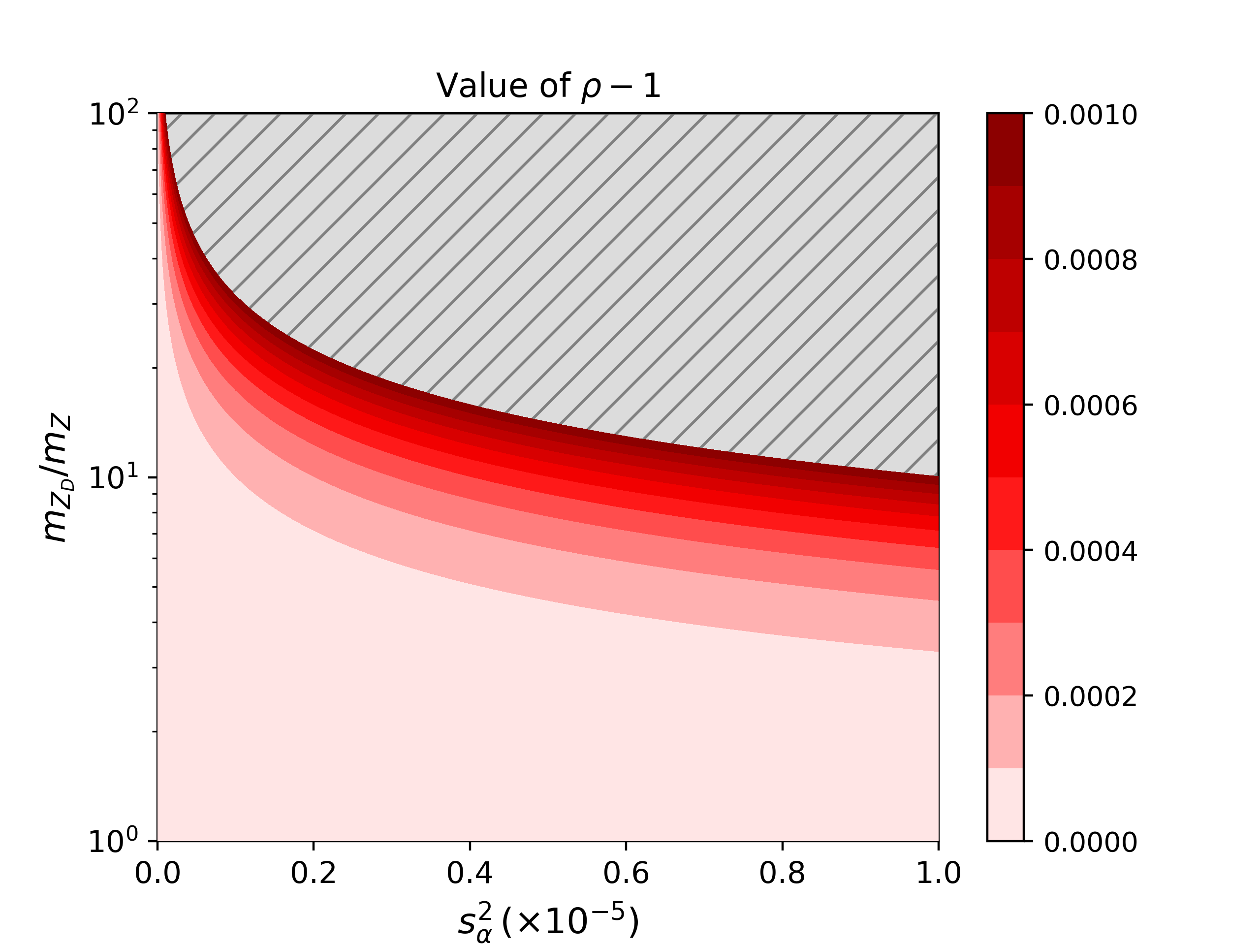
Figure 1: Impact of eq. (108) on the $(s_{\alpha}^{2},\,m_{Z_{D}}/m_{Z})$ plane, for $\rho-1\in[0,1]\times 10^{-3}$. The gray area corresponds to $\rho-1>10^{-3}$

For a given value of $\rho-1$, eq. (108) defines a line in the $(s_{\alpha}^{2},\,m_{Z_{D}}/m_{Z})$ plane, where $s_{\alpha}\equiv\sin{\alpha}$. As an example, let us take $\rho-1\in[0,1]\times 10^{-3}$, as in fig. 1, where the gray area corresponds to $\rho-1>10^{-3}$. We see that, for small values of $\rho-1$, there is a large allowed region, including very large values of $m_{Z_{D}}/m_{Z}$ for small values of $s_{\alpha}^{2}$.

Fig. 2 shows the same plane, but allowing for negative values, $\rho-1\in[-6,10]\times 10^{-4}$. We see that large values of $s_{\alpha}^{2}$ would only be possible if $m_{Z_{D}}$ were almost degenerate with $m_{Z}$. In contrast, very small values of $m_{Z_{D}}/m_{Z}$ require very small values for $s_{\alpha}^{2}$.

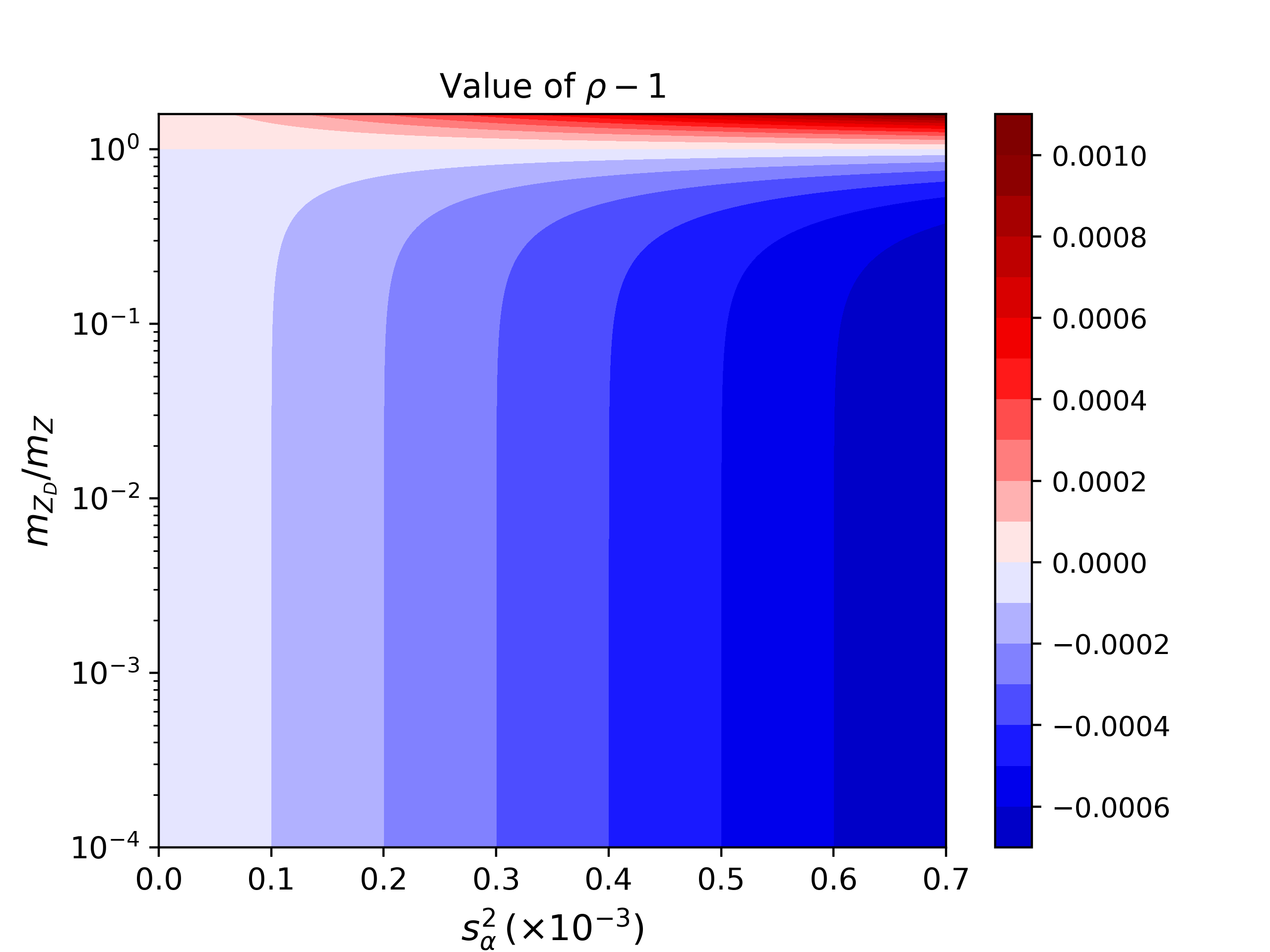
Figure 2: Impact of eq. (108) on the $(s_{\alpha}^{2},\,m_{Z_{D}}/m_{Z})$ plane, for $\rho-1\in[-6,10]\times 10^{-4}$.

Although $\rho=1$ in the Standard Model, $\rho-1$ is negative in the SU(2)${}_{L}\times$U(1)${}_{Y}\times$U(1)${}_{Y^{\prime}}$ model if $m_{Z_{D}}<m_{Z}$. For example, when $\epsilon\ll 1$ and $1-\delta^{2}\sim\mathcal{O}(1)$, it follows that

$$\rho-1\simeq\frac{t_{W}^{2}\epsilon^{2}}{\delta^{2}-1}\,.$$ (109)

Similarly, in the SU(2)${}_{L}\times$U(1)${}_{Y}\times$U(1)${}_{Y^{\prime}}$ model, $\rho-1$ is positive if $m_{Z_{D}}>m_{Z}$.

It is noteworthy that not all models with an extra $Z_{D}$ boson must have $\rho\sim 1$ if $\epsilon\ll 1$, as explained in appendix B. More generally, the elements of the squared mass matrix $\mathcal{M}_{ZZ_{D}}^{2}$ [see eq. (68)] can be related to $\rho$ by using eqs. (79)–(81) and (108). One then obtains:

$$m_{Z^{0}}^{2} = \rho m_{Z}^{2}\,,$$ (110)

$$m_{X}^{2} = \left[\frac{\cos^{2}\alpha(\rho-1)+\sin^{2}\alpha}{\rho-\cos^{2}\alpha}\right]m_{Z_{D}^{2}}=\left(1+\frac{\rho-1}{\tan^{2}\alpha}\right)m_{Z}^{2}\,,$$ (111)

$$m_{XZ}^{2} = (1-\rho)\frac{m_{Z}^{2}}{\tan\alpha}\,.$$ (112)

Any one of the above equations could serve as a definition of $\rho$ in an SU(2)${}_{L}\times$U(1)${}_{Y}\times$U(1)${}_{Y^{\prime}}$ model. For example, employing eq. (112) in the model presented in section 6.1 yields:

$$\rho=\frac{1}{1-\xi\eta t_{W}\epsilon\tan\alpha}\,.$$ (113)

By measuring the $Z\bar{f}f$ interactions and separately determining a value of $\tan\alpha$, one can extract a measurement of $\rho$ in the context of the dark-$Z$ model of section 6.1.

All results presented in section 6.2 involve tree-level parameters. In order to perform a more complete phenomenological study in which the parameters of the model are constrained by precision electroweak observables, one must include the effects of radiative loop corrections. For example, some of the dominant one-loop effects, which can be parameterized by the oblique parameters $S$, $T$, and $U$ Peskin:1991sw , have been incorporated in the analysis of the implications of generalized $Z$–$Z^{\prime}$ mixing in ref. Babu:1997st , More recently, the one-loop radiative corrections to $m_{W}$ in an SU(2)${}_{L}\times$U(1)${}_{Y}\times$U(1)${}_{Y^{\prime}}$ model have been examined in ref. Peli:2023fyb . A more careful treatment of the radiative corrections to the results obtained in this section and the resulting phenomenological consequences, which lie beyond the scope of the tree-level analysis of this work, are currently under investigation and will be reported in a future publication.

6.3 Using unitarity as a consistency test

The model presented in section 6.1 has also been analyzed in ref. Foguel:2022unm . In footnote 3, we noted errors in two of the expressions given in ref. Foguel:2022unm . One way to confirm the presence of such errors is by testing the model for consistency with unitarity, using eq. (89).

For example, eqs. (A.18)–(A.20) of ref. Foguel:2022unm exhibit the neutral vector boson squared masses and the mixing angle $\alpha$ under the assumptions that $|\epsilon|\ll 1$ and $\delta^{2}\ll 1$,

$$m_{Z}^{2}\stackrel{{\scriptstyle\rm?}}{{=}}m_{Z^{0}}^{2}\left(1+\epsilon^{2}t_{W}^{2}\right)\,,$$ (114)

$$m_{Z_{D}}^{2}\stackrel{{\scriptstyle\rm?}}{{=}}\delta^{2}m_{Z^{0}}^{2}\left(1-\epsilon^{2}t_{W}^{2}\right)\,,$$ (115)

$$\sin^{2}\alpha\stackrel{{\scriptstyle\rm?}}{{=}}\epsilon^{2}t^{2}_{W}\,.$$ (116)

Consequently, eqs. (90)–(94) yield:

$$g_{W^{+}W^{-}\gamma}^{2}=g^{2}s_{W}^{2}\,,$$ (117)

$$g_{W^{+}W^{-}Z}^{2}\stackrel{{\scriptstyle\rm?}}{{=}}g^{2}c_{W}^{2}(1-\epsilon^{2}t_{W}^{2})\,,$$ (118)

$$g_{W^{+}W^{-}Z_{D}}^{2}\stackrel{{\scriptstyle\rm?}}{{=}}g^{2}c_{W}^{2}\,\epsilon^{2}t_{W}^{2}\,,$$ (119)

$$g_{W^{+}W^{-}h}^{2}=g^{2}m_{W}^{2}c_{h}^{2}\,,$$ (120)

$$g_{W^{+}W^{-}S^{0}}^{2}=g^{2}m_{W}^{2}s_{h}^{2}\,,$$ (121)

after employing eq. (116). In the equations above, we have used the $\stackrel{{\scriptstyle\rm?}}{{=}}$ notation to indicate expressions that were obtained using an inconsistent expansion in $\epsilon$ and $\delta$ given in ref. Foguel:2022unm , where some terms of $\mathcal{O}(\epsilon^{2}\delta^{2})$ were improperly discarded. This inconsistency becomes evident when evaluating the unitarity sum rule given by eq. (89) using the results of eqs. (117)–(121), which yields

$$m_{W}^{2}-m_{Z^{0}}^{2}(c_{W}^{2}+s_{W}^{2}\epsilon^{2}\delta^{2})+\mathcal{O}\left(\epsilon^{4}\right)\stackrel{{\scriptstyle\rm?}}{{=}}0\,.$$ (122)

As expected, the $\mathcal{O}(\epsilon^{0})$ term in eq. (122) vanishes in light of eq. (63) [cf. eq. (98)]. However, a consistent expansion in $\epsilon$ and $\delta$ should yield exactly zero on the left-hand side of eq. (122) rather than nonzero terms of $\mathcal{O}(\epsilon^{2})$ and $\mathcal{O}(\epsilon^{4})$, respectively.

The impact of the inconsistent expansion in $\epsilon$ and $\delta$ can also be exhibited by computing $\rho^{\prime}$, which was defined in eq. (106). Using eqs. (114)–(116), we obtain

$$\rho^{\prime}=\left(\frac{m_{Z}^{2}}{m^{2}_{Z^{0}}}\cos^{2}\alpha+\frac{m_{Z_{D}}^{2}}{m^{2}_{Z^{0}}}\sin^{2}\alpha\right)^{-1}\stackrel{{\scriptstyle\rm?}}{{=}}1-\epsilon^{2}t_{W}^{2}\delta^{2}+\mathcal{O}\left(\epsilon^{4}\right)\,,$$ (123)

which differs from the expected result of $\rho^{\prime}=1$ by a term of $\mathcal{O}(\epsilon^{2})$. Hence, we conclude that the expansions exhibited in eqs. (114)–(116), which were employed in ref. Foguel:2022unm , violate tree-level unitarity. In a correct analysis, eqs. (118) and (119) should be replaced by eqs. (99) and (100), respectively. Likewise, eqs. (114) and (115) should be replaced by eqs. (85) and (86), respectively, and eq. (116) should be replaced by

$$\sin^{2}\alpha=\frac{\epsilon^{2}t_{W}^{2}}{(1-\delta^{2})^{2}}+\mathcal{O}(\epsilon^{4})\,,$$ (124)

in light of eqs. (87) and (88). After making these substitutions, the unitarity sum rule given by eq. (89) is restored, and the condition $\rho^{\prime}=1$ is satisfied exactly.

This exercise shows the power of the unitarity relations in probing the consistency of a given model and/or the approximations chosen.

7 Conclusions

The requirement of tree-level unitarity yields sum rules among the couplings of a given theory. The corresponding sum rules in electroweak models with an arbitrary scalar sector based on the Standard Model gauge group SU(2)${}_{L}\times$U(1)_Y have been previously obtained in refs. Gunion:1990kf ; Bento:2017eti ; Bento:2018fmy . In this paper, we have expanded the results given in the existing literature by considering models with an enlarged electroweak gauge group, SU(2)${}_{L}\times$U(1)${}_{Y}\times$U(1)${}_{Y^{\prime}}$. We have derived sum rules involving gauge bosons and scalar bosons, and we have obtained additional sum rules that include the couplings of gauge bosons and scalar bosons to fermions. In particular, we found an orthogonality of seemingly unrelated couplings, extending results presented in ref. Bento:2017eti ; Bento:2018fmy for multi-Higgs doublet models with the Standard Model electroweak gauge group.

It is instructive to apply the unitarity sum rules obtained in this paper to a concrete extended electroweak model. Thus, we considered an SU(2)${}_{L}\times$U(1)${}_{Y}\times$U(1)${}_{Y^{\prime}}$ gauge group which has been employed in the literature to provide a model for a dark sector that consists of a new gauge boson (which has been called either a dark $Z^{\prime}$ or a dark photon) that is feebly coupled to the Standard Model via kinetic mixing. The dark $Z^{\prime}$ can then be used to mediate the interactions of a new fermion or scalar that is neutral with respect to the Standard Model gauge group and hence is a candidate for dark matter. In analyzing the SU(2)${}_{L}\times$U(1)${}_{Y}\times$U(1)${}_{Y^{\prime}}$ model described above, we have provided exact analytical results as well as approximate results that are obtained to first and second order in the kinetic mixing parameter. We then demonstrate how the unitarity sum rules can be used to provide consistency checks on these results (which allows one to expose errors that have appeared in the literature due to inconsistent expansions).

Finally, we have introduced a parameter $\rho^{\prime}$ of the SU(2)${}_{L}\times$U(1)${}_{Y}\times$U(1)${}_{Y^{\prime}}$ model that serves as the analog of the $\rho$ parameter of the Standard Model. Whereas the tree-level value for $\rho$ in the Standard Model is $\rho=1$, this latter result is modified in the SU(2)${}_{L}\times$U(1)${}_{Y}\times$U(1)${}_{Y^{\prime}}$ model, whereas the tree-level value of $\rho^{\prime}=1$ is maintained. In this analysis, it is important to define the tree-level value of the weak mixing angle $\theta_{W}$ in terms of $m_{W}$, $\alpha_{\rm EM}$ and the Fermi constant $G_{F}$ in order to apply the same definition of $\theta_{W}$ to both the SU(2)${}_{L}\times$U(1)_Y and SU(2)${}_{L}\times$U(1)${}_{Y}\times$U(1)${}_{Y^{\prime}}$ models. Having done so, one can then relate the definitions of $\rho$ and $\rho^{\prime}$, to physical observables of the SU(2)${}_{L}\times$U(1)${}_{Y}\times$U(1)${}_{Y^{\prime}}$ model. These results can be applied to models of dark photons, such as those in refs. Curtin:2014cca ; Babu:1997st ; Foguel:2022unm , or to more specific studies of dark matter, such as ref. Mondino:2020lsc .

Appendix A Comparison of notation between this paper and others

For the convenience of the reader, we provide a comparison of the notation employed in section 6 with that of ref. Babu:1997st in table 2.

Parameters	This paper	ref. Babu:1997st
sine of the weak angle	$s_{W}$	$\hat{s}_{W}$
kinetic mixing term	$\epsilon$	$-\hat{c}_{W}\sin\chi$
$X$ field rescaling factor	$\eta$	$1/\cos\chi$
squared mass of $Z^{0}$ interaction-eigenstate	$m_{Z^{0}}^{2}$	$\hat{M}_{Z}^{2}$
squared mass of $\hat{X}$ interaction-eigenstate	$\delta^{2}m_{Z^{0}}^{2}$	$\hat{M}_{Z^{\prime}}^{2}$
$Z^{0}$–$X$ squared mass mixing angle	$\alpha$	$\xi$

Table 2: Comparison between the parameters in this paper and those of ref. Babu:1997st .

To obtain the physical mass eigenstates of the neutral gauge boson, the first step is to perform a field redefinition to obtain canonical kinetic energy terms (CK) for the neutral gauge fields. One then constructs the $3\times 3$ squared mass matrix of the neutral gauge bosons. It is straightforward to identify the eigenstate with zero eigenvalue (corresponding to the photon), thereby reducing the relevant neutral gauge boson squared mass matrix to a $2\times 2$ matrix. In the final step, this matrix is diagonalized to obtain the mass-eigenstate fields identified as the $Z$ boson of the SM and the dark $Z$ boson. Schematically, the notation for the fields used in this paper as compared to those of ref. Babu:1997st is indicated below:

$$\text{This paper:}\quad\left(W^{3},\hat{B},\hat{X}\right)\xrightarrow{\rm CK}\left(W^{3},B,X\right)\xrightarrow{\rm Photon}\left(A,Z^{0},X\right)\xrightarrow{\rm Mass}\left(A,Z,Z_{D}\right)\,,$$

$$\text{ref.\leavevmode\nobreak\ \cite[cite]{\@@bibref{Authors Phrase1YearPhrase2}{Babu:1997st}{\@@citephrase{(}}{\@@citephrase{)}}}:}\quad\left(W^{3},\hat{B},\hat{Z^{\prime}}\right)\xrightarrow{\rm CK}\left(W^{3},B,Z^{\prime}\right)\xrightarrow{\rm Photon}\left(A,\hat{Z},Z^{\prime}\right)\xrightarrow{\rm Mass}\left(A,Z_{1},Z_{2}\right)\,.$$ (125)

Note that the model analyzed in ref. Babu:1997st is slightly more general than the one considered here, since the former allows for the new scalar $S$ to have nonzero hypercharge $Y$. Setting the latter to zero corresponds to setting $\delta\hat{M}^{2}=0$ in the notation of ref. Babu:1997st . Moreover, ref. Babu:1997st defines one further field by

$$\hat{A}=\hat{s}_{W}W^{3}+\hat{c}_{W}\hat{B}\,.$$ (126)

This definition is not needed in section 6, and thus we do not make use of it.

Appendix B Algebraic conditions for $\rho^{\prime}=1$

The toy model introduced in section 6 is one of many examples of theories with a tree level value of $\rho^{\prime}=1$. More generally, consider a scalar extended SU(2)${}_{L}\times$U(1)_Y electroweak model, where each scalar multiplet (with weak isospin $T$ and U(1)_Y hypercharge $Y$) satisfies

$$T(T+1)=3Y^{2}\,.$$ (127)

Such models naturally yield $\rho=1$ at tree-level, independently of the values of the neutral scalar field vacuum expectation values.

If we extend the electroweak gauge group to SU(2)${}_{L}\times$U(1)${}_{Y}\times$ U(1)${}_{Y^{\prime}}$, then we must assign U(1)${}_{Y^{\prime}}$ quantum numbers to all the scalar fields. As a concrete example, suppose we consider a scalar sector that contains the SM Higgs doublet field and a second scalar multiplet with gauge quantum numbers $(T,Y,Y^{\prime})$. Then, the squared mass matrix previously obtained in eq. (68) is modified as follows:

$$\mathcal{M}^{2}_{ZZ_{D}}=m_{Z^{0}}^{2}\begin{pmatrix}1-\frac{g^{2}\delta^{2}\left[T(T+1)-3Y^{2}\right]}{2c_{W}^{2}g_{D}^{2}}&\ \ \times\\ \times&\ \ \times\end{pmatrix}\,,$$ (128)

where the matrix elements denoted by $\times$ above are not relevant for this discussion. In particular, the matrix element explicitly exhibited in eq. (128) does not depend on $Y^{\prime}$ and thus can be identified with $m_{Z^{0}}=m_{W}/c_{W}$ when eq. (127) is satisfied. Because the definition of $\rho^{\prime}$ makes use of the relation $m_{Z^{0}}c_{W}=m_{W}$ with $m_{Z^{0}}$ as defined in eq. (63), the analysis of section 6.2.4 implies that $\rho^{\prime}=1$ at tree level when (127) is satisfied, independently of the values of the neutral scalar field vacuum expectation values.

In the toy model introduced in section 6, the SU(2)${}_{L}\times$U(1)${}_{Y}\times$ U(1)${}_{Y^{\prime}}$ gauge quantum numbers of the scalar field $S$ are $(T,Y,Y^{\prime})=(0,0,1)$. In this case, eq. (128) reduces to the squared mass matrix obtained in eq. (68), and we obtain $\rho^{\prime}=1$ as advertised. Moreover, in this simple model, the tree-level value of $\rho\sim 1$ [cf. eq. (109)] because the off-diagonal element of eq. (68) were proportional to the small kinetic mixing parameter $\epsilon$. This latter result does not persist in more general models where eq. (127) is satisfied and $\rho^{\prime}=1$ is obtained. To illustrate this point, consider a modification of the toy model examined in section 6 in which $\epsilon=0$ and $S$ is replaced by a scalar field with gauge quantum numbers $(T,Y,Y^{\prime})$ such that eq. (127) is satisfied. In this case, the squared mass matrix previously obtained in eq. (68) is modified as follows:

$$\mathcal{M}^{2}_{ZZ_{D}}=m_{Z^{0}}^{2}\begin{pmatrix}1&\ \ -\displaystyle\frac{g\,Y\,\delta^{2}}{c_{W}g_{D}}\\[12.0pt] -\displaystyle\frac{g\,Y\,\delta^{2}}{c_{W}g_{D}}&\ \ \delta^{2}\end{pmatrix}\,.$$ (129)

Because this matrix is not diagonal, $\sin\alpha$ is now determined by $v_{D}/v$ and $g_{D}$. In this case, eq. (108) shows that the tree-level value of $\rho$ can deviate significantly from 1, since there is no reason for $\sin\alpha$ to be particularly small.

References

- (1) C.H. Llewellyn Smith, High-Energy Behavior and Gauge Symmetry, Phys. Lett. B 46 (1973) 233.
- (2) J.M. Cornwall, D.N. Levin and G. Tiktopoulos, Uniqueness of spontaneously broken gauge theories, Phys. Rev. Lett. 30 (1973) 1268.
- (3) J.M. Cornwall, D.N. Levin and G. Tiktopoulos, Derivation of Gauge Invariance from High-Energy Unitarity Bounds on the s Matrix, Phys. Rev. D 10 (1974) 1145.
- (4) H.A. Weldon, The Effects of Multiple Higgs Bosons on Tree Unitarity, Phys. Rev. D 30 (1984) 1547.
- (5) J.F. Gunion, H.E. Haber and J. Wudka, Sum rules for Higgs bosons, Phys. Rev. D 43 (1991) 904.
- (6) J. Brod and M. Gorbahn, The Penguin in Generic Extensions of the Standard Model, JHEP 09 (2019) 027 [1903.05116].
- (7) F. Bishara, J. Brod, M. Gorbahn and U. Moldanazarova, Generic one-loop matching conditions for rare meson decays, JHEP 07 (2021) 230 [2104.10930].
- (8) B.W. Lee, C. Quigg and H.B. Thacker, The Strength of Weak Interactions at Very High-Energies and the Higgs Boson Mass, Phys. Rev. Lett. 38 (1977) 883.
- (9) B.W. Lee, C. Quigg and H.B. Thacker, Weak Interactions at Very High-Energies: The Role of the Higgs Boson Mass, Phys. Rev. D 16 (1977) 1519.
- (10) B. Grinstein, C.W. Murphy, D. Pirtskhalava and P. Uttayarat, Theoretical Constraints on Additional Higgs Bosons in Light of the 126 GeV Higgs, JHEP 05 (2014) 083 [1401.0070].
- (11) M.P. Bento, H.E. Haber, J.C. Romão and J.P. Silva, Multi-Higgs doublet models: physical parametrization, sum rules and unitarity bounds, JHEP 11 (2017) 095 [1708.09408].
- (12) M.P. Bento, H.E. Haber, J.C. Romao and J.P. Silva, Multi-Higgs doublet models: the Higgs-fermion couplings and their sum rules, JHEP 10 (2018) 143 [1808.07123].
- (13) I.F. Ginzburg and I.P. Ivanov, Tree level unitarity constraints in the 2HDM with CP violation, hep-ph/0312374.
- (14) B. Grinstein, C.W. Murphy and P. Uttayarat, One-loop corrections to the perturbative unitarity bounds in the CP-conserving two-Higgs doublet model with a softly broken symmetry, JHEP 06 (2016) 070 [1512.04567].
- (15) I.F. Ginzburg and I.P. Ivanov, Tree-level unitarity constraints in the most general 2HDM, Phys. Rev. D 72 (2005) 115010 [hep-ph/0508020].
- (16) S. Kanemura and K. Yagyu, Unitarity bound in the most general two Higgs doublet model, Phys. Lett. B 751 (2015) 289 [1509.06060].
- (17) M.P. Bento, J.C. Romao and J.P. Silva, Unitarity bounds for all symmetry-constrained 3HDMs, JHEP 08 (2022) 273 [2204.13130].
- (18) L.B. Okun, Limits of electrodynamics: paraphotons?, Sov. Phys. JETP 56 (1982) 502.
- (19) P. Galison and A. Manohar, Two ’s or not two s?, Phys. Lett. B 136 (1984) 279.
- (20) B. Holdom, Two U(1)’s and Epsilon Charge Shifts, Phys. Lett. B 166 (1986) 196.
- (21) R. Foot and X.-G. He, Comment on – mixing in extended gauge theories, Phys. Lett. B 267 (1991) 509.
- (22) D. Curtin, R. Essig, S. Gori and J. Shelton, Illuminating Dark Photons with High-Energy Colliders, JHEP 02 (2015) 157 [1412.0018].
- (23) D.C. Kennedy and B.W. Lynn, Electroweak Radiative Corrections with an Effective Lagrangian: Four Fermion Processes, Nucl. Phys. B 322 (1989) 1.
- (24) B. Holdom, Oblique electroweak corrections and an extra gauge boson, Phys. Lett. B 259 (1991) 329.
- (25) Y. Cheng, X.-G. He, F. Huang, J. Sun and Z.-P. Xing, Dark photon kinetic mixing effects for the CDF W-mass measurement, Phys. Rev. D 106 (2022) 055011 [2204.10156].
- (26) P. Langacker and M.-x. Luo, Constraints on additional bosons, Phys. Rev. D 45 (1992) 278.
- (27) K.S. Babu, C.F. Kolda and J. March-Russell, Implications of generalized Z - Z-prime mixing, Phys. Rev. D 57 (1998) 6788 [hep-ph/9710441].
- (28) P. Langacker, The Physics of Heavy Gauge Bosons, Rev. Mod. Phys. 81 (2009) 1199 [0801.1345].
- (29) P. Fayet, Parity violation effects induced by a new gauge boson, Phys. Lett. B 96 (1980) 83.
- (30) P. Fayet, Effects of the Spin 1 Partner of the Goldstino (Gravitino) on Neutral Current Phenomenology, Phys. Lett. B 95 (1980) 285.
- (31) H. An, M. Pospelov, J. Pradler and A. Ritz, Direct Detection Constraints on Dark Photon Dark Matter, Phys. Lett. B 747 (2015) 331 [1412.8378].
- (32) M. Backovic, A. Mariotti and D. Redigolo, Di-photon excess illuminates Dark Matter, JHEP 03 (2016) 157 [1512.04917].
- (33) P. Ilten, Y. Soreq, M. Williams and W. Xue, Serendipity in dark photon searches, JHEP 06 (2018) 004 [1801.04847].
- (34) H. Davoudiasl, H.-S. Lee and W.J. Marciano, ‘Dark’ Z implications for Parity Violation, Rare Meson Decays, and Higgs Physics, Phys. Rev. D 85 (2012) 115019 [1203.2947].
- (35) A. Alves, S. Profumo and F.S. Queiroz, The dark portal: direct, indirect and collider searches, JHEP 04 (2014) 063 [1312.5281].
- (36) S. Bilmis, I. Turan, T.M. Aliev, M. Deniz, L. Singh and H.T. Wong, Constraints on Dark Photon from Neutrino-Electron Scattering Experiments, Phys. Rev. D 92 (2015) 033009 [1502.07763].
- (37) M. Lindner, F.S. Queiroz, W. Rodejohann and X.-J. Xu, Neutrino-electron scattering: general constraints on and dark photon models, JHEP 05 (2018) 098 [1803.00060].
- (38) F. del Aguila, J. de Blas, P. Langacker and M. Perez-Victoria, Impact of extra particles on indirect limits, Phys. Rev. D 84 (2011) 015015 [1104.5512].
- (39) P. Ko, Y. Omura and C. Yu, A Resolution of the Flavor Problem of Two Higgs Doublet Models with an Extra Symmetry for Higgs Flavor, Phys. Lett. B 717 (2012) 202 [1204.4588].
- (40) H. Davoudiasl, H.-S. Lee, I. Lewis and W.J. Marciano, Higgs Decays as a Window into the Dark Sector, Phys. Rev. D 88 (2013) 015022 [1304.4935].
- (41) P. Ko, Y. Omura and C. Yu, Higgs phenomenology in Type-I 2HDM with Higgs gauge symmetry, JHEP 01 (2014) 016 [1309.7156].
- (42) G. Arcadi, T. Hugle and F.S. Queiroz, The Dark Rises via Kinetic Mixing, Phys. Lett. B 784 (2018) 151 [1803.05723].
- (43) H. Davoudiasl, W.J. Marciano, R. Ramos and M. Sher, Charged Higgs Discovery in the W plus ”Dark” Vector Boson Decay Mode, Phys. Rev. D 89 (2014) 115008 [1401.2164].
- (44) A.L. Foguel, G.M. Salla and R.Z. Funchal, (In)Visible signatures of the minimal dark abelian gauge sector, JHEP 12 (2022) 063 [2209.03383].
- (45) R. L. Workman et al. [Particle Data Group Collaboration], Review of Particle Physics, PTEP 2022 (2022) 083C01.
- (46) G. Altarelli, R. Casalbuoni, S. De Curtis, N. Di Bartolomeo, F. Feruglio and R. Gatto, Improved bounds on extended gauge models from new LEP data, Phys. Lett. B 263 (1991) 459.
- (47) M.E. Peskin and T. Takeuchi, Estimation of oblique electroweak corrections, Phys. Rev. D 46 (1992) 381.
- (48) Z. Péli and Z. Trócsányi, Precise prediction for the mass of the W boson in gauged U(1) extensions of the standard model, Phys. Rev. D 108 (2023) L031704 [2305.11931].
- (49) C. Mondino, M. Pospelov, J.T. Ruderman and O. Slone, Dark Higgs Dark Matter, Phys. Rev. D 103 (2021) 035027 [2005.02397].