Cooperative Hardware-Prompt Learning for
Snapshot Compressive Imaging

Abstract

Snapshot compressive imaging emerges as a promising technology for acquiring real-world hyperspectral signals. It uses an optical encoder and compressively produces the 2D measurement, followed by which the 3D hyperspectral data can be retrieved via training a deep reconstruction network. Existing reconstruction models are trained with a single hardware instance, whose performance is vulnerable to hardware perturbation or replacement, demonstrating an overfitting issue to the physical configuration. This defect limits the deployment of pre-trained models since they would suffer from large performance degradation when are assembled to unseen hardware. To better facilitate the reconstruction model with new hardware, previous efforts resort to centralized training by collecting multi-hardware and data, which is impractical when dealing with proprietary assets among institutions. In light of this, federated learning (FL) has become a feasible solution to enable cross-hardware cooperation without breaking privacy. However, the naive FedAvg is subject to client drift upon data heterogeneity owning to the hardware inconsistency. In this work, we tackle this challenge by marrying prompt tuning with FL to snapshot compressive imaging for the first time and propose an federated hardware-prompt learning (FedHP) method. Rather than mitigating the client drift by rectifying the gradients, which only takes effect on the learning manifold but fails to touch the heterogeneity rooted in the input data space, the proposed FedHP globally learns a hardware-conditioned prompter to align the data distribution, which serves as an indicator of the data inconsistency stemming from different pre-defined coded apertures. Extensive experiments demonstrate that the proposed method well coordinates the pre-trained model to indeterminate hardware configurations. We hope this work will inspire future attempts to solve practical problems of snapshot compressive imaging.

1 Introduction

Snapshot compressive imaging (SCI) [38] has recently emerged as a representative computational imaging technology. Coded aperture snapshot spectral imaging (CASSI) [9] system falls in the field of SCI and has gained increasing research attention by efficiently capturing real-world hyperspectral data with a low cost. It takes the 3D hyperspectral signal and produces the 2D measurement, which could be then retrieved by deep reconstruction networks [3, 4, 23, 12, 26, 11, 27, 31] with high-fidelity. So far, the learning prototype of deep reconstruction models is limited to an inflexible scenario, where each model is exclusively compatible with a unique hardware configuration, i.e., a pre-defined coded aperture. Despite their remarkable performance, the pre-trained models are vulnerable to the subtle variation of the coded aperture, presenting an overfitting issue toward the hardware. In practice, this issue greatly hinders the further deployment of pre-trained reconstruction models. Whenever the physical set-up of CASSI experiences inevitable/unknown perturbations, or the hardware instance is directly replaced, the deep reconstruction model needs to be re-trained, which is not only inefficient but also will require expensive computational resources.

To solve the Hardware Overfitting issue of the reconstruction models, previous effort [32] resorts to the centralized learning solutions. (1) A naive treatment is to jointly train a reconstruction model with a series of hardware configurations, i.e., coded apertures. As shown in Fig. 1 right, this solution enhances the generalization ability of reconstruction ($>0.5$dB$+$) by comparison. However, the performance on unseen coded apertures of reconstruction is still non-guaranteed since the model only learns to fit limited number of coded apertures in a purely data-driven manner. Followed by, GST [32] (namely, Self-tuning in Fig. 1) advances the learning by explicitly approximating the posterior distribution of coded apertures in a variational Bayesian framework. Despite the significant performance boost, it poses a strict probabilistic constraint to the hardware, i.e., it is only compatible with the coded apertures drawing from the same posterior. Moreover, both solutions fall in the venue of centralized learning by presuming that hardware instances and hyperspectral data are publicly available. However, the optical system of CASSI and data samples are generally proprietary assets in practice, bearing strict privacy policy constraints.

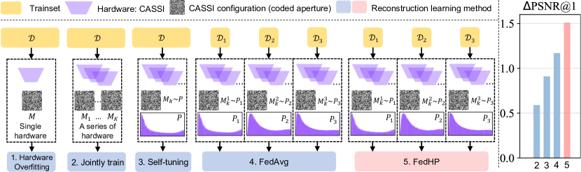
Figure 1: Comparison of existing hyperspectral reconstruction model learning strategies. (1) Training the model with the single hardware instance leads to Hardware Overfitting issue. Both (2) Jointly train and (3) Self-tuning [32] are centralized training solutions. Compared with (4) FedAvg [25], the proposed (5) FedHP better coordinates hardware instances with different configurations. We compare the performance gain of different methods over (1) on the right.

Federated learning [16, 20, 33] enables cross-device/silo collaboration with preserving the privacy. In this work, we resort to FL for improving the robustness of reconstruction to different hardware. By observation, FedAvg outperforms the centralized learning. However, it suffers from degraded performance under heterogeneous data [10, 17]. The heterogeneity in SCI substantially stems from the hardware, since CASSI compressively prepends the data for the network training. Thus, one coded aperture governs a specific input data distribution. We explicitly consider two heterogeneity scenarios. (1) A general case is that the heterogeneity simply attributes to different coded apertures across clients. (2) Besides, we take a step further to consider that heterogeneity owes to the distinct distributions of coded apertures across different clients (see Fig. 1 FedAvg), which pictures the situation where cross-silo hardware instances origin from different manufacturing agents.

To approach the heterogeneity issue, in this work, we propose a Federated Hardware-Prompt (FedHP) learning framework. Existing methods handle the heterogeneity by regularizing the global/local gradients [17, 21], which only take effect on the learning manifold but fail to touch the heterogeneity rooted in the input data space. Motivated by this point, FedHP implicitly observes diverse hardware configurations of different clients and learns a shared prompter to adaptively tune the input data representation, inspired by the nascent research direction of visual prompt learning [14, 1]. By taking the coded aperture as input, the prompter is expected to modify the local data representation into a shared space, thereby bridging the distribution gap between clients. Besides, since prompt learning takes effect on the pre-trained models, FedHP instantiates the reconstruction backbones with locally well-trained models and keeps them frozen throughout the learning, which potentially improves the efficiency than directly optimizing and aggregating the reconstruction backbones in FL. We summarize the contributions as follows:

• We discuss the practical limitations of hardware overfitting and privacy concern in existing hyperspectral reconstruction learning solutions. We introduce FedHP to coordinate the pre-trained reconstruction models to distinct hardware configurations. To the best knowledge, this is the first attempt to discuss the power of FL for solving the practical problem persistent in the field of SCI.

• We uncover and define two types of data heterogeneity scenarios stemming from distinct CASSI configurations. A hardware-conditioned prompt learning method is proposed as a unified solution to solve the data distribution shift across clients. The proposed method provides an orthogonal perspective in handling the heterogeneity to the common practices of regularizing optimization.

• Extensive experiments demonstrate that FedHP outperforms both centralized learning methods and classic federated learning treatments under two heterogeneous scenarios. By collecting the heterogeneous data from a series of real CASSI systems, we provide a benchmark to inspire the future works to this novel research direction of hardware collaboration in SCI.

2 Method

In this section, we firstly introduce the preliminary knowledge of hyperspectral image reconstruction in Section 2.1. We then discuss the centralized learning solutions in Section 2.2 and challenges of federated learning for SCI in Section 2.3. We finally elaborate the proposed FedHP in Section 2.4.

2.1 Preliminary Knowledge

Coded aperture snapshot spectral imaging (CASSI) recently emerges as a promising instrument for hyperspectral signal acquisition. Given the real-world hyperspectral signal $\mathbf{X}\in\mathbb{R}^{H\times W\times N_{\lambda}}$, where $N_{\lambda}$ denotes the number of spectral channels, CASSI performs the compression with the physical coded apterture $\mathbf{M}$ of the size $H\times W$, i.e., $\mathbf{M}_{hw}\in[0,1]$. Accordingly, the encoding process produces a 2D measurement $\mathbf{Y}^{\mathbf{M}}\in\mathbb{R}^{H\times(W+\Delta)}$, where $\Delta$ represents the shifting

$$\mathbf{Y}^{\mathbf{M}}=\sum_{n_{\lambda}=1}^{N_{\lambda}}\mathbf{X}^{\prime}(:,:,{n_{\lambda}})\odot\mathbf{M}+\mathbf{\Omega},\ \ \ \mathbf{X}^{\prime}(h,w,n_{\lambda})=\mathbf{X}(h,w+d(\lambda-\lambda^{*}),n_{\lambda}),$$ (1)

where $\odot$ denotes the pixel-wise multiplication and $\mathbf{\Omega}$ presents the measurement noise. For each spectral wavelength $\lambda$, the corresponding signal $\mathbf{X}(:,:,n_{\lambda})$ is shifted according to the function $d(\lambda-\lambda^{*})$ by referring to the pre-defined anchor wavelength $\lambda^{*}$, such that $\Delta=d(N_{\lambda}-1)$. Following the optical encoder, recent practices train a deep reconstruction network $f(\cdot)$ to retrieve the hyperspectral data $\widehat{\mathbf{X}}\in\mathbb{R}^{H\times W\times N_{\lambda}}$ by taking the 2D measurement $\mathbf{Y}^{\mathbf{M}}$ as input. We define the initial training dataset of the hyperspectral signal as $\mathcal{D}$ and the corresponding dataset for the reconstruction as $\mathcal{D^{\mathcal{M}^{*}}}$

$$\mathcal{D}=\{\mathbf{X}_{i}\}^{i=N}_{i=1},~{}~{}\mathcal{D}^{\mathbf{M}^{*}}=\{\mathbf{Y}_{i}^{\mathbf{M}^{*}},\mathbf{X}_{i}\}^{i=N}_{i=1},$$ (2)

where $\mathbf{X}_{i}$ serves as the ground truth and $\mathbf{Y}_{i}^{\mathbf{M}^{*}}$ is governed by the physical coded aperture $\mathbf{M}^{*}$. The reconstruction model finds the local optimum that minimizes the mean squared loss

$$\widehat{\theta}=\mathop{\arg\min}_{\theta}\frac{1}{N}\sum^{N}_{i=1}||f(\theta;\mathbf{Y}_{i}^{\mathbf{M}^{*}})-\mathbf{X}_{i}||^{2}_{2},\ \ \ \widehat{\mathbf{X}}_{i}=f(\widehat{\theta};\mathbf{Y}_{i}^{\mathbf{M}^{*}}),$$ (3)

where $\theta$ expresses all learnable parameters in the reconstruction model. Thanks to the sophisticated network designs [3, 12, 26], pre-trained reconstruction model demonstrates promising performance when is compatible with a single encoder set-up, where the measurement in training and testing phases are both produced by the same hardware using a fixed coded aperture of $\mathbf{M}^{*}$.

However, previous work [32] uncovered that most existing reconstruction models experience large performance descent (e.g., $>2$dB in terms of PSNR) when handling the input measurements encoded by a different coded aperture $\mathbf{M}^{\dagger}$ from training, i.e., $\mathbf{M}^{\dagger}\neq\mathbf{M}^{*}$. This is because the coded aperture $\mathbf{M}^{*}$ implicitly affects the learning as shown by Eq. (3). We denote this scenario as Hardware Overfitting since the reconstruction models is highly sensitive to the hardware configuration of coded aperture and are hardly compatible with the unseen optical system in the testing phase. To devise the reconstruction network with a new coded aperture $\mathbf{M}^{\dagger}$, a simple solution is to retrain the model with corresponding dataset $\mathcal{D}^{\mathbf{M}^{\dagger}}=\{\mathbf{Y}_{i}^{\mathbf{M}^{\dagger}},\mathbf{X}_{i}\}^{i=N}_{i=1}$and then test upon $\mathbf{M}^{\dagger}$ accordingly. However, retraining does not solve this issue, upon which the reconstruction model is still vulnerable to the slight variation of coded aperture. Besides, drastic computation overhead is introduced. Both of the reasons limit the practical significance of pre-trained deep reconstruction models. In this work, we tackle this challenge by encouraging the robustness of the reconstruction networks toward different hardware configurations, i.e., coded apertures.

2.2 Centralized Learning in SCI

Jointly Train. To solve the above problem, Jointly train serves as a naive solution to train a model with data jointly collected upon a series of hardware. Assuming there are total number of $K$ hardware with different coded apertures, i.e., $\mathbf{M}_{1},\mathbf{M}_{2},...,\mathbf{M}_{K}$. Each hardware produces a training dataset upon $\mathcal{D}$ as $\mathcal{D}^{\mathbf{M}_{k}}=\{\mathbf{Y}_{i}^{\mathbf{M}_{k}},\mathbf{X}_{i}\}_{i=1}^{i=N}$. The joint training dataset for reconstruction is

$$\mathcal{D}^{\mathbf{M}_{1\sim K}}=\mathcal{D}^{\mathbf{M}_{1}}\cup\mathcal{D}^{\mathbf{M}_{2}}\cup\ldots\cup\mathcal{D}^{\mathbf{M}_{K}},$$ (4)

where different coded apertures can be regarded as hardware-driven data augmentation treatments toward the hyperspectral data representation. The reconstruction model will be trained with the same mean squared loss privided in Eq. (3) upon $\mathcal{D}^{\mathbf{M}_{1\sim K}}$. Previous attempts [32] demonstrated that jointly learning indeed brings performance boost for testing measurements upon $\mathbf{M}_{k}$. However, Jointly train only collects limited number of coded apertures, which empowers the robustness in a pure data-driven manner. The performance of reconstruction model on unseen coded apertures is still non-guaranteed. Besides, this method adopts a set of fixed learnable parameters to handle different hardware, failing to adaptively cope with the hardware discrepancies.

Self-tuning. Following Jointly train, recent work of Self-tuning [32] recognizes the coded aperture that plays the role of hyperprameter of the reconstruction network, and develops a hyper-net to explicitly model the posterior distribution of the coded aperture by observing $\mathcal{D}^{\mathbf{M}_{1\sim K}}$. Specifically, the hyper-net $h(\sigma;\mathbf{M}_{k})$ approximates $P(\mathbf{M}|\mathcal{D}^{\mathbf{M}_{1\sim K}})$ by minimizing the Kullback–Leibler divergence between this posterior and a variational distribution $Q(\mathbf{M})$ parameterized by $\sigma$. Compared with Jointly train, Self-tuning learns to adapt to different coded apertures and appropriately calibrates the reconstruction network during training, even if there are unseen coded apertures. However, the variational Bayesian learning poses a strict distribution constraint to the sampled coded apertures, which limits the scope of Self-tuning under the practical setting. Besides, it requires an additional hyper-net for the calibration beyond the reconstruction, leading to burdensome computation overhead.

To sum up, both of the Jointly train and Self-tuning are representative solutions of centralized learning, where the dataset $\mathcal{D}$ and hardware instances with $\mathbf{M}_{1},...,\mathbf{M}_{K}$ from different institutions are publicly available. Such a setting has two-fold limitations. (1) Centralized learning does not take the privacy concern into consideration. In practice, both the hardware instances and hyperspectral dataset are proprietary assets of institutions and thus, corresponding hardware configuration and data information sharing is subject to the rigorous policy constraint. (2) Existing centralized learning methods mainly consider the scenario where coded apertures are sampled from the same distribution, i.e., hardware origin from the same source, which is problematic when it comes to the coded aperture distribution inconsistency especially in the cross-silo case. Considering the above challenges, in the following, we resort to the federated learning (FL) methods. To the best knowledge, this is the first attempt of FL in solving the robustness of reconstruction model toward different hardware.

2.3 Federated Learning in SCI

FedAvg. We firstly tailor FedAvg [25], into snapshot compressive imaging. Specifically, we exploit a practical setting of cross-silo learning in snapshot compressive imaging. Suppose there are $C$ clients, where each client is packaged with a group of hardware following a specific distribution of $P_{c}$

$$\mathbf{M}^{c}_{k}\sim P_{c},$$ (5)

where $\mathbf{M}^{c}_{k}$ represents $k$-th sampled coded aperture in $c$-th client. For simplicity, we use $\mathbf{M}^{c}$ to denote arbitrary coded aperture sample in $c$-th client. Based on the hardware, each client computes a paired dataset $\mathcal{D}^{\mathbf{M}^{c}}$ from the local hyperspectral dataset $\mathcal{D}_{c}$

$$\mathcal{D}_{c}=\{\mathbf{X}_{i}\}^{i=N_{c}}_{i=1},\ \ \ \mathcal{D}^{\mathbf{M}^{c}}=\{\mathbf{Y}_{i}^{\mathbf{M}^{c}},\mathbf{X}_{i}\}^{i=N_{c}}_{i=1},\ \ \ \mathbf{M}^{c}\sim P_{c},$$ (6)

where $N_{c}$ represents the number of hyperspectral data in $\mathcal{D}_{c}$. The local learning objective is

$$\ell_{c}(\theta)=\frac{1}{N}\sum^{N}_{i=1}||\widehat{\mathbf{X}}_{i}-\mathbf{X}_{i}||^{2}_{2},$$ (7)

where $\widehat{\mathbf{X}}_{i}=f(\widehat{\theta};\mathbf{Y}_{i}^{\mathbf{M}^{c}}),\ \mathbf{M}^{c}\sim P_{c}$, we use $\theta$ to denote the learnable parameters of reconstruction model at a client. FedAvg learns a global model $\theta_{G}$ without sharing the hyperspectral signal dataset $\mathcal{D}_{c}$, $\mathcal{D}^{\mathbf{M}^{c}}$, and $\mathbf{M}^{c}$ across different clients. Specifically, the global learning objective $\ell_{G}(\theta)$ is

$$\ell_{G}(\theta)=\sum_{c=1}^{C^{\prime}}\alpha_{c}\ell_{c}(\theta),$$ (8)

where $C^{\prime}$ denotes the number of clients that participate in the current global round and $\alpha_{c}$ represents the aggregation weight. Compared with the centralized learning solutions, FedAvg not only bridges the local hyperspectral data for a more accurate reconstruction, but also collaborates different hardware instances across multiple institutions for a more generalized reconstruction model learning. However, FedAvg shows limitations in two-folds. (1) It has been shown that FedAvg delivers degraded performance under the heterogeneous data [17, 18, 10]. (2) Directly training and aggregating the reconstruction backbones would introduce prohibitive computation. In the following, we will firstly introduce the data heterogeneity in snapshot compressive imaging. Then we develop a Federated Hardware-Prompt (FedHP) method to tackle the heterogeneity without optimizing the backbones.

Data Heterogeneity. We firstly consider the data heterogeneity stems from the different coded apertures samples, i.e., hardware instances. According to Section 2.1, CASSI samples the hyperspectral signal $\mathbf{X}_{i}$ from $\mathcal{D}=\{\mathbf{X}_{i}\}_{i=1}^{i=N}$ and encodes it into a 2D measurement $\mathbf{Y}_{i}^{\mathbf{M}}$, which constitutes $\mathcal{D}^{\mathbf{M}}$ and further serves as the input data for the reconstruction model. To this end, the modality of $\{\mathbf{Y}^{\mathbf{M}}_{i}\}^{i=1}_{i=N}$ is vulnerable to the coded aperture variation. A single coded aperture $\mathbf{M}$ defines a unique input data distribution for the reconstruction, i.e., $\mathbf{Y}_{i}^{\mathbf{M}}\sim P_{\mathbf{M}}(\mathbf{Y}_{i}^{\mathbf{M}})$. For arbitrary distinct coded apertures, we have $P_{\mathbf{M}^{*}}(\mathbf{Y}_{i}^{\mathbf{M}^{*}})\neq P_{\mathbf{M}^{\dagger}}(\mathbf{Y}_{i}^{\mathbf{M}^{\dagger}})\ \texttt{if}\ \mathbf{M}^{*}\neq\mathbf{M}^{\dagger}$. In federated learning, data heterogeneity persistently exists since there is no identical coded aperture across different clients. We name this heterogeneous scenario as Hardware shaking, which potentially can attribute to physical perturbations such as lightning distortion or optical platform fluttering.

We take a step further to consider the other type of data heterogeneity stemming from the distinct distributions of coded apertures . As formulated in Eq. (6), each client collects a coded aperture assemble following the distribution $P_{c}$ for $c$-th client. We have $P_{c}$ differs from one another, i.e., $P_{c1}\neq P_{c2}$ for $c1\neq c2$, $c1,c2\in\{1,...,C\}$. We name this heterogeneous scenario as Manufacturing discrepancy, where hardware instances from different clients (institutions) are produced by distinct manufacturing agencies, so that the distribution $P_{c1}$ and $P_{c2}$ drastically differs as demonstrated in Fig. 1. This turns out to be a more challenging scenario than Hardware shaking. As presented in Section 3.2, classic federated learning methods, e.g., FedProx [21] and SCAFFOLD [17] hardly converge in this setting. By comparison, the proposed method enables an obvious performance boost.

2.4 FedHP: Federated Hardware-Prompt Learning

Hardware-Prompt Learning. Bearing the heterogeneous issue, previous efforts [21, 17] mainly focus on rectifying the global/local gradients upon training, which only takes effect on the learning manifold but fail to touches the heterogeneity rooted in the input data space. Since we explicitly uncover and determine two types of the heterogeneity in snapshot compressive imaging stemming from the hardware inconsistency (Section. 2.3), we resort to reshape the encoded data representations of different clients to a shared space. This can be achieved by collaboratively learning the input data alignment given different coded apertures. In light of the visual prompt tuning advances in large models [24, 2], we devise a hardware-conditioned prompt network in the following.

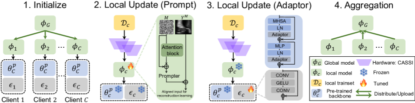
Figure 2: Learning process of FedHP. We take one global round as an example, which consists of (1) Initialize, (2) Local Update (Prompt), (3) Local Update (Adaptor), and (4) Aggregation. For each client, the reconstruction backbone ($\theta_{c}^{p}$), is initialized as pre-trained model upon local training dataset $\mathcal{D}_{c}$ and kept as frozen throughout the training. The prompt net upon hardware configuration, i.e., coded aperture, takes effect on the input data of reconstruction, i.e., $\mathbf{Y}^{\mathbf{M}}$. Adaptors are introduced to enhance the learning, where $\epsilon_{c}$ denotes the parameters of all adaptors.

As shown in the Step 2 of Fig. 2, given the input data $\{\mathbf{Y}_{i}^{\mathbf{M}}\}_{i=1}^{i=N}$ of the reconstruction, the prompt network aligns the input samples, i.e., measurements $\mathbf{Y}^{\mathbf{M}_{i}}$, by adding a prompter conditioned on the hardware configuration. Let $\Phi(\phi;\mathbf{M})$ denote the prompt network (e.g., attention block) parameterized by $\phi$ and $\mathbf{Y}^{\mathbf{M}}_{i}$ is produced upon coded aperture $\mathbf{M}$. Then the resulting input sample is aligned as

$$\mathbf{Y}^{\mathbf{M}}_{i}=\mathbf{Y}^{\mathbf{M}}_{i}+\Phi(\phi;\mathbf{M}).$$ (9)

In the proposed method, the prompt network collaborates different clients with inconsistent hardware configurations. It takes effect by implicitly observing and collecting diverse coded aperture samples of all clients, and jointly learns to react to different hardware settings. The prompter regularizes the input data space and achieves the goal of coping with heterogeneity sourcing from hardware.

Training. As shown in Fig. 2, we demonstrate the training process of proposed FedHP by taking one global round as an example. Since the prompt learning takes effect on pre-trained models, we prepend the $c$-th backbone parameters with the pre-trained model $\theta_{c}^{p}$ on local data $\mathcal{D}^{\mathbf{M}^{c}}$ with Eq. (7). The global prompt network $\phi_{G}$ is randomly initialized and distributed to the $c$-th client

$$\phi_{c}\leftarrow\phi_{G},\ c=1,...,C^{\prime},$$ (10)

where $\phi_{c}$ is the local prompt network and $C^{\prime}$ denotes the number of clients participated in current global round. To enable better response of the pre-trained backbone toward the aligned input data space, we also introduce the adaptors into the transformer backbone. As shown in Fig. 2 Step 3, we show the architecture of the proposed adaptor, which is a CONV-GELU-CONV structure governed by a residual connection. We insert the adaptors behind the LN layers throughout the network.

We then perform local update in each global round. It is composed of two stages. Firstly, we update the local prompt network $\phi_{c}$ for $S_{p}$ iterations, all the other learnable parameters of backbone and adaptors are frozen. The loss then becomes

$$\ell_{c}=\frac{1}{N}\sum^{N}_{i=1}||f(\theta^{p}_{c},\epsilon_{c};\mathbf{Y}_{i}^{\mathbf{M}^{c}}+\Phi(\mathbf{M}^{c}))-\mathbf{X}_{i}||^{2}_{2},$$ (11)

where we use $\epsilon_{c}$ to represent learnable parameters of all adaptors for $c$-th client. Secondly, we tune the adaptors for another $S_{b}$ iterations. Both of the pre-trained backbone and prompt network are frozen. The loss of $c$-th client shares the same formulation as Eq. (11). After the local update, FedHP uploads and aggregates the learnable parameters $\phi_{c}$, $c=1,...,C$ of prompt network. Since the proposed method does not require to optimize and communicate the reconstruction backbones, the underlying cost is drastically reduced considering the marginal model size of prompt network and adptors compared with the backbone, which potentially serves as a supplied benefit of FedHP.

Compared with FedAvg, FedHP adopts the hardware-conditioned prompt to explicitly align the input data representation and handles the data distribution shift attributing to the coded aperture inconsistency (hardware shaking) or coded aperture distribution discrepancy (manufacturing discrepancy), as introduced in Section 2.3.

3 Experiments

3.1 Implementation details

Dataset. Following existing practices [4, 23, 11, 12], we adopt the benchmark training dataset of CAVE [37], which is composed of $32$ hyperspectral images with the spatial size as $512\times 512$. Data augmentation techniques of rotation, flipping are employed. For the federated learning, we equally split the training dataset according to the number of clients $C$. The local training dataset are kept and accessed confidentially by corresponding clients. We employ the widely-used simulation testing dataset for the quantitative evaluation, which consists of ten $256\times 256\times 28$ hyperspectral images collected from KAIST [6]. Besides, we use the real testing data with spatial size of $660\times 660$ collected by a SD-CASSI system [26] for the perceptual evaluation considering the real-world perturbations.

Table 1: PSNR(dB)/SSIM performance on the simulation benchmark testing dataset. We consider the data heterogeneity stem from hardware shaking. We report mean${}_{\pm\texttt{std}}$ among 100 trials.

Scene	FedAvg [25]		FedProx [21]		SCAFFOLD [17]		FedGST [32]		FedHP (ours)
	PSNR	SSIM	PSNR	SSIM	PSNR	SSIM	PSNR	SSIM	PSNR	SSIM
1	31.98±0.19	0.8938±0.0025	31.85±0.21	0.8903±0.0028	31.78±0.24	0.8886±0.0025	32.02±0.14	0.8918±0.0018	32.31±0.19	0.9026±0.0020
2	30.49±0.21	0.8621±0.0041	29.85±0.22	0.8516±0.0037	29.81±0.19	0.8473±0.0031	30.13±0.20	0.8519±0.0038	30.78±0.19	0.8746±0.0034
3	31.78±0.23	0.9088±0.0019	30.80±0.23	0.8968±0.0017	30.92±0.17	0.8961±0.0014	31.19±0.22	0.8975±0.0015	31.62±0.25	0.9109±0.0018
4	39.39±0.23	0.9559±0.0018	39.41±0.22	0.9601±0.0013	39.32±0.20	0.9565±0.0011	38.98±0.27	0.9513±0.0020	39.78±0.29	0.9633±0.0017
5	28.70±0.16	0.8821±0.0044	28.14±0.16	0.8765±0.0036	28.08±0.14	0.8742±0.0032	28.53±0.16	0.8743±0.0041	28.92±0.17	0.8935±0.0039
6	30.53±0.30	0.9054±0.0025	30.04±0.23	0.9054±0.0024	29.87±0.21	0.9011±0.0019	30.29±0.21	0.8949±0.0022	30.77±0.22	0.9172±0.0019
7	30.01±0.20	0.8811±0.0027	29.60±0.20	0.8718±0.0026	29.63±0.19	0.8708±0.0027	29.89±0.18	0.8786±0.0024	30.44±0.19	0.8884±0.0024
8	28.60±0.31	0.8880±0.0023	27.93±0.20	0.8845±0.0018	27.74±0.31	0.8802±0.0018	28.35±0.19	0.8752±0.0016	28.56±0.32	0.8957±0.0021
9	31.45±0.15	0.9012±0.0019	31.29±0.15	0.8961±0.0019	31.22±0.14	0.8929±0.0014	30.80±0.12	0.8880±0.0021	31.34±0.13	0.9043±0.0023
10	29.04±0.13	0.8751±0.0022	28.48±0.15	0.8671±0.0035	28.59±0.13	0.8626±0.0028	28.51±0.13	0.8578±0.0024	29.12±0.13	0.8835±0.0021
Avg.	31.21±0.10	0.8959±0.0017	30.76±0.10	0.8900±0.0016	30.71±0.09	0.8872±0.0013	30.85±0.11	0.8858±0.0017	31.35±0.10	0.9033±0.0014

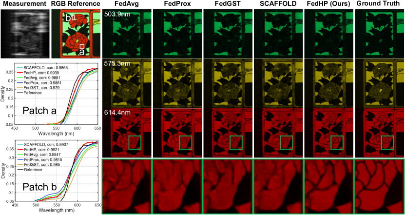
Figure 3: Reconstruction results on simulation data. The density curves compares the spectral consistency of different methods to the ground truth. We use the same coded aperture for all methods.

Hardware. We collect CASSI systems from three agencies, each of which offers a series of coded apertures that corresponds to a unique distributions as presented by federated settings in Fig. 2. No identical coded apertures exists among all systems. As introduced in Section 2.3, two types of data heterogeneity scenarios are discussed. For the case of manufacturing discrepancy, we directly assign CASSI systems from one source to form a client. Besides, we simulate the scenario of hardware shaking by distributing coded apertures from one source to different clients.

Implementation details. We adopt the popular transformer backbone, MST-S [3] for the reconstruction. Besides, the prompt network is instantiated by a SwinIR [22] block. Limited by the real-world hardware, we set the number of clients as $3$ in federated learning. We empirically find that collaborate such amount of clients can be problematic for popular federated learning methods under the very challenging scenario of data heterogeneity (see Section 3.2). For FL methods, we update all clients throughout the training, i.e., $C^{\prime}=C=3$. For the proposed method, we pre-train the client backbones from scratch for $4\times 10^{4}$ iterations on their local data. Notably, the total training iterations of different methods are kept as $1.25\times 10^{5}$ for a fair comparison. The batch is set as $12$. We set the initial learning rate for both of the prompt network and adaptor as $\alpha_{p}=\alpha_{b}=1\times 10^{-4}$ with step schedulers, i.e., half annealing every 2$\times$10⁴ iterations. We train the model with an Adam [19] optimizer ($\beta_{1}=0.9,\beta_{2}=0.999$). We implement the proposed method with PyTorch [28] on an NVIDIA A100 GPU.

Compared Methods. We compare the proposed FedHP with mainstream federated learning methods, including FedAvg [25], FedProx [21], and SCAFFOLD [17]. Besides, GST [32] paves the way for the robustness of the reconstruction toward multiple hardware. Thereby, we take a step further to incorporate this method under the federated setting, dubbed as FedGST. Notably, all the compared methods require to train and aggregate the client backbones without a prompter or adaptor introduced. By comparison, FedHP updates and shares the prompt network, outperforming the others despite an unfair comparison (see Section 3.2). We adopt PSNR and SSIM [34] for the quantitative evaluation.

3.2 Performance

Simulation Results. We quantitatively compare different methods in Table 1 by considering the data heterogeneity stems from hardware shaking. FedHP performs better than the classic federated learning methods. By comparison, FedProx and SCAFFOLD only allows sub-optimal performance, which uncovers the limitations of rectifying the gradient directions in this challenging task. Besides, FedGST works inferior than FedHP, since FedGST approximates the posterior and expects coded apertures strictly follows the identical distribution, which can not be guaranteed in practice. In Fig. 3, we visualize the reconstruction results with sampled wavelengths. FedHP not only enables a more granular retrieval on unseen coded aperture, but also maintains a promising spectral consistency.

Challenging Scenario of Heterogeneity. We further consider a more challenging scenario of manufacturing discrepancy, where the data heterogeneity is highly entangled to the large gap among the coded aperture distributions. We compare different methods in Table 2. By observation, all methods experience large performance degradation, among which FedProx and SCAFFOLD becomes nearly ineffective. Intuitively, it is hard to concur the clients under the large distribution gap, while directly adjusting the input data space better tackles the problem.

Real Results. In Fig. 4, we visually compare the FedAvg with FedHP on the real data. Specifically, both methods are evaluated under an unseen hardware configuration, i.e., coded aperture from an uncertain distribution. The proposed method introduces less distortions among different wavelengths. Such an observation endorses FedHP a great potential in collaborating CASSI systems practically.

Table 2: PSNR(dB)/SSIM performance on the simulation testing dataset. We consider the data heterogeneity stem from manufacturing discrepancy. We report mean${}_{\pm\texttt{std}}$ among 100 trials.

Scene	FedAvg [25]		FedProx [21]		SCAFFOLD [17]		FedGST [32]		FedHP (ours)
	PSNR	SSIM	PSNR	SSIM	PSNR	SSIM	PSNR	SSIM	PSNR	SSIM
1	29.15±0.09	0.8392±0.0065	23.01±0.11	0.5540±0.0069	22.99±0.13	0.5535±0.0066	29.46±0.65	0.8344±0.0067	30.37±0.70	0.8628±0.0084
2	28.28±0.10	0.8102±0.0052	20.91±0.08	0.4486±0.0052	20.89±0.09	0.4474±0.0055	27.89±0.36	0.7733±0.0068	28.67±0.38	0.8160±0.0072
3	28.42±0.11	0.8464±0.0083	17.57±0.11	0.4621±0.0082	17.58±0.12	0.4608±0.0083	28.45±0.50	0.8363±0.0073	29.81±0.68	0.8771±0.0066
4	36.93±0.27	0.9369±0.0036	23.08±0.25	0.4856±0.0036	23.00±0.30	0.4848±0.0038	36.12±0.50	0.9181±0.0050	37.37±0.53	0.9395±0.0032
5	25.84±0.07	0.8037±0.0069	18.99±0.07	0.4316±0.0082	18.99±0.06	0.4301±0.0065	26.21±0.52	0.7988±0.0081	27.47±0.73	0.8487±0.0011
6	27.28±0.04	0.8655±0.0041	19.10±0.04	0.4077±0.0041	19.10±0.04	0.4063±0.0042	27.52±0.49	0.8384±0.0048	28.31±0.45	0.8649±0.0050
7	26.81±0.09	0.8042±0.0094	20.15±0.09	0.4903±0.0093	20.14±0.09	0.4883±0.0098	26.88±0.57	0.7957±0.0073	28.29±0.81	0.8298±0.0108
8	25.77±0.05	0.8473±0.0030	19.89±0.07	0.4402±0.0031	19.89±0.06	0.4395±0.0039	26.22±0.44	0.8206±0.0029	26.54±0.45	0.8470±0.0054
9	28.30±0.09	0.8541±0.0074	18.33±0.11	0.4285±0.0071	18.30±0.11	0.4269±0.0078	27.74±0.48	0.8199±0.0073	29.36±0.63	0.8536±0.0054
10	26.04±0.12	0.8075±0.0035	20.06±0.12	0.3461±0.0036	20.03±0.13	0.3451±0.0036	25.72±0.22	0.7433±0.0046	26.78±0.26	0.8111±0.0076
Avg.	28.63±0.07	0.8496±0.0041	20.85±0.07	0.5405±0.0059	20.00±0.09	0.4374±0.0040	28.24±0.39	0.8177±0.0045	28.98±0.23	0.8481±0.0054

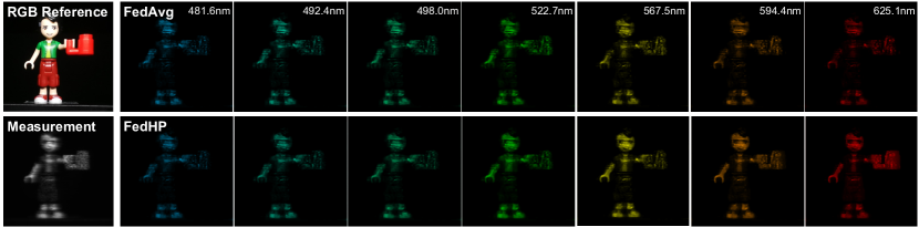
Figure 4: Visualization of reconstruction results on real data. Six representative wavelengths are selected. We use the same unseen coded aperture for both FedAvg and FedHP.

Table 3: Ablation study and complexity analysis under the Hardware shaking. The PSNR (dB)/SSIM are computed among 100 testing trials. We report the number of learnable parameters of different methods and report the accumulative training time of all clients (e.g., $C=3$).

Prompter	Adaptor	FL	PSNR	SSIM	$\#$params (M)	GMACs	Training (days)
✓	✓	✗	30.75±0.11	0.8890±0.0015	0.27	12.78	2.86
✓	✗	✓	31.09±0.10	0.8996±0.0017	0.15	11.01	2.68
✗	✓	✓	19.19±0.01	0.2303±0.0008	0.12	2.87	2.54
✓	✓	✓	31.35±0.10	0.9033±0.0014	0.27	12.78	2.86

3.3 Model Discussion

We conduct model discussion in Table 3. Specifically, we accumulate the total cost (e.g., number of parameters, GMACs, and training time) of all clients in a federated system.

Without FL. We firstly consider a scenario that trains three clients independently without FL. For a fair comparison, each client pre-trains the backbone by using the same procedure as FedHP and are then enhanced with a prompt network and adaptors for efficient fine-tuning. By comparison, FedHP enables an obvious improvement ($0.6$dB) by implicitly sharing the hardware and data.

Without Prompter or Adaptor. We then investigate the effectiveness of the promter and adaptor to the reconstruction, respectively. By observation, directly removing the adaptor leads to limited performance descent. However, only updating and sharing the adaptor hardly helps the training. This indicates that modifying the input data space brings more benefit than adapting the learning manifold. This is determined by the fact that learning manifold is highly correlated with the coded apertures.

4 Related Work

Hyperspectral Image Reconstruction. Hyperspectral image reconstruction methods retrieves the 3D hyperspectral data from 2D measurements produced by CASSI. Learning deep reconstruction models [3, 4, 23, 12, 26, 11, 27] has been the forefront among recent efforts due to high-fidelity reconstruction and high-efficiency. Among them, MST [3] devises the first transformer backbone by computing spectral attention. By observation, existing reconstruction learning strategies mainly considers the compatibility toward a single hardware instance. The leared model can be highly sensitive to the variation of hardware. To tackle this prctical challenge, GST [32] paves the way by proposing a variational Bayesian learning treatment.

Federated Learning. Federated learning [16, 20, 33] collaborates across clients without sharing the privacy-sensitive assets. However, FL learning suffers from client drift across clients attributing to the data heterogeneity issue. One mainstream [17, 21, 36, 13, 29] mainly focus on regularizing the global/local gradients. As another direction, personalized FL methods [7, 5, 8, 30, 15] propose to fine-tune the global model for better adaptability on clients. However, customizing the global model on client data sacrifices the underlying robustness upon data distribution shift [35, 15], which contradicts with our goal of emphasizing the generality across hardware and thus is not considered. In addition, it seems that the power of federated learning have not yet been exploited in the filed of SCI. In this work, the proposed method fills this research gap of adopting federated learning to coordinate hardware.

5 Conclusions

In this work, we have exploited the robustness of the reconstruction model toward the distinct configurations of CASSI in snapshot compressive imaging. We developed Federated Hardware-Prompt (FedHP) by marrying the nascent technology of prompt tuning with federated learning. Specifically, we uncovered and defined two types of data heterogeneity stemming from the hardware and devised an hardware-conditioned prompter to align the input data space. The proposed method serves as a first attempt to demonstrate the feasibility of coordinating multiple hardware. Future works may theoretically exploit the convergence of FedHP under both heterogenious settings. Besides, the behavior of FedHP under a large number of clients (e.g., $>100$) remains to be explored. We hope the proposed work will inspire more research from both FL and SCI community on the challenging problem of CASSI collaboration.

Appendix

Appendix A Social Impact

This work develops a federated learning treatment to enable the collaboration of the CASSI systems with different hardware configurations. The proposed method will practically encourage the cross-institution collaborations with emerging optical system designs engaged. By improving the robustness of the pre-trained reconstruction software backend toward optical encoders, this work will help expedite the efficient and widespread deployment of the deep models on sensors or platforms.

Appendix B Performance on More Clients

Table 4: Performance of FedAvg and FedHP under different number of clients.

$\#$Clients	FedAvg [25]		FedHP
	PSNR	SSIM	PSNR	SSIM
3	31.21±0.10	0.8959±0.0017	31.35±0.10	0.9033±0.0014
4	31.06±0.10	0.8955±0.0018	31.33±0.13	0.9023±0.0018
5	31.05±0.10	0.9025±0.0014	31.32±0.19	0.9029±0.0019

In this section, we discuss the effectiveness of the proposed FedHP on more clients (i.e., $C=4,5$). Specifically, we adopt the same training dataset for different settings and evenly split it according to the number of clients. As shown in Table 4, FedHP consistently outperforms the FedAvg, which indicates that the proposed collaborative learning solution is more robuts to the number of clients. Besides, we observe that FedHP remains a relative stable performance on different number of clients. By comparison, FedAvg suffers from an obvious performance descent when $C=4,5$. Intuitively, FedHP collaboratively learns a global prompter for a client-specific input data space adaptation, which can effectively solve the distribution gap induced by different hardware instances. However, FedAvg learns a shared backbone for different data distributions, which inevitably suffers from the client drift. This issue will be strengthened when more clients participate in the learning. We leave the exploitation of very large number of clients (e.g., $C=100$) into the future works.

Appendix C Algorithm

The learning procedure of proposed FedHP is provided in Algorithm 1. Let us take one global round for example, the learning can be divided into four stages. (1) Initializing the global prompt network from scratch and then distributing it to local clients. Then instantiating the client backbones with the pre-trained models upon the local training dataset. The adaptors are also randomly initialized for a better adaptation of the pre-trained backbones to the aligned input data representation. (2) Local updating of the prompt network, during which all the other learnable parameters in the system are kept fixed. (3) Local updating of the adaptors. Notably, the parameters of the adaptors is only updated and maintained in local. (4) Global aggregation of the local prompt networks.

Algorithm 1 FedHP Training Algorithm

1:Number of global rounds $T$; Number of clients $C$; Number of client subset $C^{\prime}$; Pre-trained models ${\theta}^{p}_{c}$, $c=1,...,C$; Number of local update iterations $S_{p}$, $S_{b}$; Random initialized parameter of prompt network $\phi_{G}$; Random initialized parameter of adaptors of $c$-th client $\epsilon_{c}$; Learning rate $\alpha_{p}$ of prompt network; Learning rate $\alpha_{b}$ of adaptors;

2:$\phi_{G},\epsilon_{c}$, $c=1,...,C$;

3:Server Executes;

4:Randomly choose a set of clients of number $C^{\prime}$;

5:for $t=1,...,T$ do

6:     for $c\in C^{\prime}$ in parallel do

7:         Send global prompt network $\phi_{G}$ to $\phi_{c}$;

8:         $\phi_{c}\leftarrow$ LocalTraining(${\theta}^{p}_{c}$, $\epsilon_{c}$, $\phi_{c}$);

9:     end for

10:     $\phi_{G}\leftarrow\sum^{c=C^{\prime}}_{c=1}\frac{|\mathcal{D}_{c}|}{|\mathcal{D}|}\phi_{c}$;

11:end for

12:return $\phi_{G}$;

13:LocalTraining(${\theta}^{p}_{c}$, $\epsilon_{c}$, $\phi_{c}$);

14:for $s=1,...,S_{p}$ do

15:     $\phi_{c}\leftarrow\phi_{c}-\alpha_{p}\nabla\ell({\theta}^{p}_{c},\epsilon_{c},\phi_{c})$ using $\ell_{c}=\frac{1}{N}\sum^{N}_{i=1}||f(\theta^{p}_{c},\epsilon_{c};\mathbf{Y}_{i}^{\mathbf{M}^{c}}+\Phi(\mathbf{M}^{c}))-\mathbf{X}_{i}||^{2}_{2}$;

16:end for

17:for $s=1,...,S_{b}$ do

18:     $\epsilon_{c}\leftarrow\epsilon_{c}-\alpha_{b}\nabla\ell({\theta}^{p}_{c},\epsilon_{c},\phi_{c})$ using $\ell_{c}=\frac{1}{N}\sum^{N}_{i=1}||f(\theta^{p}_{c},\epsilon_{c};\mathbf{Y}_{i}^{\mathbf{M}^{c}}+\Phi(\mathbf{M}^{c}))-\mathbf{X}_{i}||^{2}_{2}$;

19:end for

20:return $\phi_{c}$ to server;

Appendix D Visualization Results

In this section, we provide more visualization results of different methods. In Figs. 5$\sim$6, we present the reconstruction results of different methods under the scenario of hardware shaking, i.e., the data heterogeneity is naively induced from the different CASSI instances across clients. FedHP enables more fine-grained details retrieval. Besides, we compare the spectral density curves on selected representative spatial regions. The higher correlation to the reference, the better spetrum consistency with the ground truth. In Figs. 7$\sim$8, we show additional real reconstruction results of FedAvg and FedHP on selected wavelengths. By comparison, FedAvg fails to reconstruct some content, while the proposed FedHP allows a more granular result.

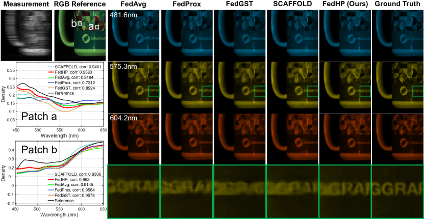
Figure 5: Reconstruction results on simulation data. The density curves compares the spectral consistency of different methods to the ground truth. We use the same coded aperture for all methods.

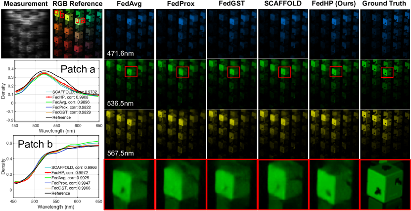
Figure 6: Reconstruction results on simulation data. The density curves compares the spectral consistency of different methods to the ground truth. We use the same coded aperture for all methods.

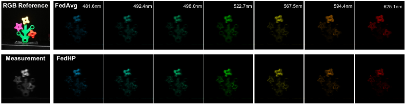
Figure 7: Visualization of reconstruction results on real data. Seven (out of $28$) representative wavelengths are selected. We use the same unseen coded aperture for both FedAvg and FedHP.

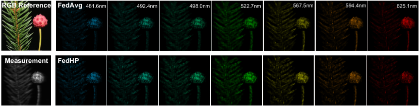
Figure 8: Visualization of reconstruction results on real data. Seven (out of $28$) representative wavelengths are selected. We use the same unseen coded aperture for both FedAvg and FedHP.

Appendix E Coded Aperture Distributions

In Figs. 9$\sim$11, we visualize the different distributions of coded apertures in distinct clients under the scenario of the distribution shift of coded apertures among different clients leads to the data heterogeneity among different local input dataset. This mimics a very challenging scenario where in different clients (e.g., research institutions), the corresponding CASSI systems source from different manufacturers. The proposed FedHP allows a potential collaboration among different institutions for the hyperspectral data acquisition for the first time despite the large distribution gap. By comparison, classic methods of FedProx [21] or SCAFFOLD [17] fail to provide reasonable retrieval results.

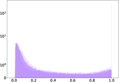
Figure 9: Distribution of Coded apertures in Client $1$ ($C=3$) under the scenario of manufacturing discrepancy. The symmetrical logarithm scale is employed for a better visualization.

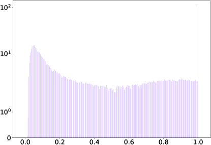
Figure 10: Distribution of Coded apertures in Client $2$ ($C=3$) under the scenario of manufacturing discrepancy. The symmetrical logarithm scale is employed for a better visualization.

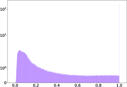
Figure 11: Distribution of Coded apertures in Client $3$ ($C=3$) under the scenario of manufacturing discrepancy. The symmetrical logarithm scale is employed for a better visualization.

References

- Bahng et al. [2022a] Hyojin Bahng, Ali Jahanian, Swami Sankaranarayanan, and Phillip Isola. Exploring visual prompts for adapting large-scale models. arXiv preprint arXiv:2203.17274, 1(3):4, 2022a.
- Bahng et al. [2022b] Hyojin Bahng, Ali Jahanian, Swami Sankaranarayanan, and Phillip Isola. Visual prompting: Modifying pixel space to adapt pre-trained models. arXiv preprint arXiv:2203.17274, 2022b.
- Cai et al. [2022a] Yuanhao Cai, Jing Lin, Xiaowan Hu, Haoqian Wang, Xin Yuan, Yulun Zhang, Radu Timofte, and Luc Van Gool. Mask-guided spectral-wise transformer for efficient hyperspectral image reconstruction. In Proceedings of the IEEE/CVF Conference on Computer Vision and Pattern Recognition, pages 17502–17511, 2022a.
- Cai et al. [2022b] Yuanhao Cai, Jing Lin, Haoqian Wang, Xin Yuan, Henghui Ding, Yulun Zhang, Radu Timofte, and Luc Van Gool. Degradation-aware unfolding half-shuffle transformer for spectral compressive imaging. arXiv preprint arXiv:2205.10102, 2022b.
- Chen and Chao [2021] Hong-You Chen and Wei-Lun Chao. On bridging generic and personalized federated learning for image classification. arXiv preprint arXiv:2107.00778, 2021.
- Choi et al. [2017] Inchang Choi, MH Kim, D Gutierrez, DS Jeon, and G Nam. High-quality hyperspectral reconstruction using a spectral prior. Technical report, 2017.
- Collins et al. [2021] Liam Collins, Hamed Hassani, Aryan Mokhtari, and Sanjay Shakkottai. Exploiting shared representations for personalized federated learning. In International Conference on Machine Learning, pages 2089–2099. PMLR, 2021.
- Fallah et al. [2020] Alireza Fallah, Aryan Mokhtari, and Asuman Ozdaglar. Personalized federated learning with theoretical guarantees: A model-agnostic meta-learning approach. Advances in Neural Information Processing Systems, 33:3557–3568, 2020.
- Gehm et al. [2007] Michael E Gehm, Renu John, David J Brady, Rebecca M Willett, and Timothy J Schulz. Single-shot compressive spectral imaging with a dual-disperser architecture. Optics express, 15(21):14013–14027, 2007.
- Hsu et al. [2019] Tzu-Ming Harry Hsu, Hang Qi, and Matthew Brown. Measuring the effects of non-identical data distribution for federated visual classification. arXiv preprint arXiv:1909.06335, 2019.
- Hu et al. [2022] Xiaowan Hu, Yuanhao Cai, Jing Lin, Haoqian Wang, Xin Yuan, Yulun Zhang, Radu Timofte, and Luc Van Gool. Hdnet: High-resolution dual-domain learning for spectral compressive imaging. In Proceedings of the IEEE/CVF Conference on Computer Vision and Pattern Recognition (CVPR), pages 17542–17551, 2022.
- Huang et al. [2021] Tao Huang, Weisheng Dong, Xin Yuan, Jinjian Wu, and Guangming Shi. Deep gaussian scale mixture prior for spectral compressive imaging. In Proceedings of the IEEE/CVF Conference on Computer Vision and Pattern Recognition (CVPR), pages 16216–16225, 2021.
- Jhunjhunwala et al. [2023] Divyansh Jhunjhunwala, Shiqiang Wang, and Gauri Joshi. Fedexp: Speeding up federated averaging via extrapolation. arXiv preprint arXiv:2301.09604, 2023.
- Jia et al. [2022] Menglin Jia, Luming Tang, Bor-Chun Chen, Claire Cardie, Serge Belongie, Bharath Hariharan, and Ser-Nam Lim. Visual prompt tuning, 2022.
- Jiang and Lin [2023] Liangze Jiang and Tao Lin. Test-time robust personalization for federated learning. In International Conference on Learning Representations, 2023.
- Kairouz et al. [2021] Peter Kairouz, H Brendan McMahan, Brendan Avent, Aurélien Bellet, Mehdi Bennis, Arjun Nitin Bhagoji, Kallista Bonawitz, Zachary Charles, Graham Cormode, Rachel Cummings, et al. Advances and open problems in federated learning. Foundations and Trends® in Machine Learning, 14(1–2):1–210, 2021.
- Karimireddy et al. [2020] Sai Praneeth Karimireddy, Satyen Kale, Mehryar Mohri, Sashank Reddi, Sebastian Stich, and Ananda Theertha Suresh. Scaffold: Stochastic controlled averaging for federated learning. In International Conference on Machine Learning, pages 5132–5143. PMLR, 2020.
- Khaled et al. [2020] Ahmed Khaled, Konstantin Mishchenko, and Peter Richtárik. Tighter theory for local sgd on identical and heterogeneous data. In International Conference on Artificial Intelligence and Statistics, pages 4519–4529. PMLR, 2020.
- Kingma and Ba [2014] Diederik P Kingma and Jimmy Ba. Adam: A method for stochastic optimization. arXiv preprint arXiv:1412.6980, 2014.
- Li et al. [2020a] Tian Li, Anit Kumar Sahu, Ameet Talwalkar, and Virginia Smith. Federated learning: Challenges, methods, and future directions. IEEE signal processing magazine, 37(3):50–60, 2020a.
- Li et al. [2020b] Tian Li, Anit Kumar Sahu, Manzil Zaheer, Maziar Sanjabi, Ameet Talwalkar, and Virginia Smith. Federated optimization in heterogeneous networks. Proceedings of Machine learning and systems, 2:429–450, 2020b.
- Liang et al. [2021] Jingyun Liang, Jiezhang Cao, Guolei Sun, Kai Zhang, Luc Van Gool, and Radu Timofte. Swinir: Image restoration using swin transformer. In Proceedings of the IEEE/CVF International Conference on Computer Vision (ICCV), pages 1833–1844, 2021.
- Lin et al. [2022] Jing Lin, Yuanhao Cai, Xiaowan Hu, Haoqian Wang, Xin Yuan, Yulun Zhang, Radu Timofte, and Luc Van Gool. Coarse-to-fine sparse transformer for hyperspectral image reconstruction. arXiv preprint arXiv:2203.04845, 2022.
- Liu et al. [2023] Pengfei Liu, Weizhe Yuan, Jinlan Fu, Zhengbao Jiang, Hiroaki Hayashi, and Graham Neubig. Pre-train, prompt, and predict: A systematic survey of prompting methods in natural language processing. ACM Computing Surveys, 55(9):1–35, 2023.
- McMahan et al. [2017] Brendan McMahan, Eider Moore, Daniel Ramage, Seth Hampson, and Blaise Aguera y Arcas. Communication-efficient learning of deep networks from decentralized data. In Artificial intelligence and statistics, pages 1273–1282. PMLR, 2017.
- Meng et al. [2020] Ziyi Meng, Jiawei Ma, and Xin Yuan. End-to-end low cost compressive spectral imaging with spatial-spectral self-attention. In European Conference on Computer Vision (ECCV), August 2020.
- Miao et al. [2019] Xin Miao, Xin Yuan, Yunchen Pu, and Vassilis Athitsos. -net: Reconstruct hyperspectral images from a snapshot measurement. In IEEE/CVF Conference on Computer Vision (ICCV), 2019.
- Paszke et al. [2017] Adam Paszke, Sam Gross, Soumith Chintala, Gregory Chanan, Edward Yang, Zachary DeVito, Zeming Lin, Alban Desmaison, Luca Antiga, and Adam Lerer. Automatic differentiation in pytorch. 2017.
- Reddi et al. [2020] Sashank Reddi, Zachary Charles, Manzil Zaheer, Zachary Garrett, Keith Rush, Jakub Konečnỳ, Sanjiv Kumar, and H Brendan McMahan. Adaptive federated optimization. arXiv preprint arXiv:2003.00295, 2020.
- T Dinh et al. [2020] Canh T Dinh, Nguyen Tran, and Josh Nguyen. Personalized federated learning with moreau envelopes. Advances in Neural Information Processing Systems, 33:21394–21405, 2020.
- Wang et al. [2022a] Jiamian Wang, Kunpeng Li, Yulun Zhang, Xin Yuan, and Zhiqiang Tao. S^ 2-transformer for mask-aware hyperspectral image reconstruction. arXiv preprint arXiv:2209.12075, 2022a.
- Wang et al. [2022b] Jiamian Wang, Yulun Zhang, Xin Yuan, Ziyi Meng, and Zhiqiang Tao. Modeling mask uncertainty in hyperspectral image reconstruction. In Computer Vision–ECCV 2022: 17th European Conference, Tel Aviv, Israel, October 23–27, 2022, Proceedings, Part XIX, pages 112–129. Springer, 2022b.
- Wang et al. [2021] Jianyu Wang, Zachary Charles, Zheng Xu, Gauri Joshi, H Brendan McMahan, Maruan Al-Shedivat, Galen Andrew, Salman Avestimehr, Katharine Daly, Deepesh Data, et al. A field guide to federated optimization. arXiv preprint arXiv:2107.06917, 2021.
- Wang et al. [2004] Zhou Wang, Alan C Bovik, Hamid R Sheikh, and Eero P Simoncelli. Image quality assessment: from error visibility to structural similarity. IEEE transactions on image processing, 13(4):600–612, 2004.
- Wu et al. [2022] Shanshan Wu, Tian Li, Zachary Charles, Yu Xiao, Ziyu Liu, Zheng Xu, and Virginia Smith. Motley: Benchmarking heterogeneity and personalization in federated learning. arXiv preprint arXiv:2206.09262, 2022.
- Xu et al. [2021] Jing Xu, Sen Wang, Liwei Wang, and Andrew Chi-Chih Yao. Fedcm: Federated learning with client-level momentum. arXiv preprint arXiv:2106.10874, 2021.
- Yasuma et al. [2010] Fumihito Yasuma, Tomoo Mitsunaga, Daisuke Iso, and Shree K Nayar. Generalized assorted pixel camera: postcapture control of resolution, dynamic range, and spectrum. IEEE transactions on image processing, 19(9):2241–2253, 2010.
- Yuan et al. [2021] Xin Yuan, David J Brady, and Aggelos K Katsaggelos. Snapshot compressive imaging: Theory, algorithms, and applications. IEEE Signal Processing Magazine, 38(2):65–88, 2021.