Abstract

We present mean horizontal branch absolute magnitudes and iron abundances for a sample of 39 globular clusters. These quantities were calculated in an unprecedented homogeneous fashion based on Fourier decomposition of ligt curves of RR Lyrae cluster members. Zero points for the luminosity calibrations are discussed. Our photometrically derived metallicities and distances compare very well with spectroscopic determinations of [Fe/H] and accurate distances obtained using Gaia and Hubble Space Telescope data. The need to distinguish between the results for RRab and RRc stars for a correct evaluation of the $M_{V}$–[Fe/H] relation is discussed. For RRab stars, the relation is non-linear, and the horizontal branch structure plays a significant role. For RRc stars, the relation remains linear and tight, and the slope is very shallow. Hence, the RRc stars seem better indicators of the parental cluster distances. Systematic time-series CCD imaging performed over the last 20 years enabled to discover and classify 330 variables in our sample of globular clusters.

1 Introduction

The Fourier light curve decomposition technique is based on the representation of the observed light curve by a series of harmonics of adequate amplitudes and displacements, $A_{k}$ and $\phi_{k}$, in an equation of the form,

$$m(t)=A_{0}+\sum_{k=1}^{N}{A_{k}\cos\left({2\pi k\over P}\leavevmode\nobreak\ (t-E)+\phi_{k}\right)},$$ (1)

where $m(t)$ is the magnitude at time $t$, $P$ is the pulsation period, and $E$ is the epoch, typically selected as the time of maximum brightness. A linear minimization routine is used to derive the best-fitting values for the amplitudes $A_{k}$ and phases $\phi_{k}$ of the sinusoidal components. The Fourier parameters, defined as $\phi_{ij}=j\phi_{i}-i\phi_{j}$ and $R_{ij}=A_{i}/A_{j}$, are computed from the amplitudes and phases of the harmonics in eq. 1. In principle, a proper combination of some of these Fourier parameters, to be determined on theoretical and/or empirical grounds, can yield appropriate physical stellar parameters. The demonstration of this fact and its practical application has taken a few decades, and it traces its origins to the pioneering work of [44], [39] and [40]. Simon employed hydrodynamic pulsation models to construct light curves and experimented with Fourier decomposition in search of useful correlations, eventually expressing that “Finally, we argue that if a reliable hydrodynamic pulsation code were available, the Fourier technique would be capable of determining masses, luminosities and temperatures of individual stars, in many cases using observations already in hand.” And, in fact, hydrodynamical models were developed in another early work by [41], where the significance of the $\phi_{31}$ parameter in the estimation of the stellar mass and luminosity of RRc stars was demonstrated.

Towards the end of the 20th century, a program aimed at calculating accurate empirical relations for the physical parameters of RR Lyrae stars was developed at the Konkoly Observatory. Soon, robust and simple empirical calibrations emerged for the determination of [Fe/H] [25] and the absolute magnitude [28] in terms of the pulsation period, yielding the Fourier $A_{1}$ and $\phi_{31}$ parameters for a large sample of RRab stars in the globular clusters of the Sculptor dwarf galaxy. The then-recent set of iron abundances [42, 32] and photometric data [31, 34] were employed.

Soon after, it was argued that some hydrodynamical pulsation models did not follow the empirical light curves [28, 29], and then empirical calibrations were preferred [30].

A thorough [Fe/H] calibration for RRc stars [35] employed a sample of 106 calibrator stars in globular clusters and rendered useful formulae for the iron abundance estimation on the Zinn–West metallicity scale [47]. More recently, a further effort to improve the accuracy of the calibrations, using high precision Kepler photometry and detailed spectroscopic iron abundances for RRab and RRc stars, was performed [36]. Twenty-six calibrators were included in the RRab calibration (nine with Blazhko modulations) and 101 calibrators for the RRc calibration.

For nearly 20 years our research group has been interested in performing extensive time-series CCD photometry in the VI bands for a sample of Galactic globular clusters. We aimed at estimating cluster mean metallicities and distances from their member RR Lyrae stars via the Fourier decomposition technique, and from other variables in a cluster when available, e.g. SX Phe via their period–luminosity (P–L) relation, or red giant semi-periodic variables near the tip of the red giant branch (RGB). Meanwhile, other aspects of the clusters under study have been addressed, such as their reddening, stellar membership and a census of their variable star populations; their periods and classifications have also been updated. As a natural by-product we discovered and classified about 330 new variables.

Numerous RR Lyrae light curve decompositions and their implied physical parameters can be found in the literature, but often different calibrations and zero points to estimate [Fe/H] and $M_{V}$ are used. For the determination of these quantities, in earlier investigations, our group also used some different equations, since we were also learning what were probably the best and most reliable calibrations. Hence, we decided to reconsider all our data and determine Fourier fits to pursue homogeneous calculations with the selected calibrations, for our entire sample of globular clusters [1]. The specific calibrations employed will be presented in Section 3.

The present paper is organized as follows. In Section 4, we summarize the resulting values of reddening, [Fe/H] and $M_{V}$ (and, hence, distance) for our sample of globular clusters and compare them with spectroscopically determined iron abundance values, while comparing the distances with well established mean distances based on Gaia and Hubble Space Telescope (HST) data. In Section 5 we will revisit the $M_{V}$–[Fe/H] correlation in light of the homogeneous set of Fourier [Fe/H] and $M_{V}$ values. We highlight the need to split the discussion of results obtained from RRab stars and those from RRc stars, as they are of an obviously different nature. In Section 6 we introduce the role of the HB structure on the $M_{V}$–[Fe/H] relation and discuss its results. Section 7 recounts briefly the census of new variables discovered in this project. Finally, in Section 8 we summarize our results and conclusions.

2 CCD Photometry based on the DIA approach

All our CCD photometry obtained over the years has been performed based on Difference Image Analysis (DIA) through the pipeline DanDIA [7]; [10]; [8]. A detailed description of the method and its caveats can be found in [9]. A good overview of all our procedures applied to the analysis of the individual clusters is found in [21] and [46].

3 The [Fe/H] and $M_{V}$ calibrations employed

3.1 The [Fe/H] calibrations

For the calculation of [Fe/H] we adopted the following calibrations:

$${\rm[Fe/H]}_{\rm J}=-5.038-5.394P+1.345\phi^{(s)}_{31},$$ (2)

and

$${\rm[Fe/H]}_{\rm ZW}=52.466P^{2}-30.075P+0.131\phi^{(c)2}_{31}-0.982\phi^{(c)}_{31}-4.198\phi^{(c)}_{31}P+2.424,$$ (3)

from [25] and [35] for RRab and RRc stars, respectively. The phases $\phi^{(c)}$ and $\phi^{(s)}$ are calculated either based on a cosine or a sine series, respectively, and they are correlated via $\phi^{(s)}=\phi^{(c)}-\pi$. The iron abundance on the [25] scale, [Fe/H]_J, can be converted to the [47] scale via [Fe/H]_J = 1.431 [Fe/H]_ZW + 0.88 [24]. All [Fe/H]_ZW values can be converted to the UVES spectroscopic scale of [13] via [Fe/H]${}_{\rm UV}=-0.413+0.130$ [Fe/H]${}_{\rm ZW}-0.356$ [Fe/H]${}_{\rm ZW}^{2}$.

We have also considered the more recent non-linear calibrations calculated by [36] for both RRab and RRc stars. These calibrations made use of high-precision Kepler photometry and spectroscopic iron abundances for 26 RRab and 101 RRc calibrators. Their resulting equations are, respectively,

$${\rm[Fe/H]_{N}}=-8.65-40.12P+5.96\phi_{31}^{(s)}(K)+6.27\phi_{31}^{(s)}(K)P-0.72\phi_{31}^{(s)}(K){{}^{2}},$$ (4)

where $\phi_{31}^{(s)}(K)=\phi_{31}^{(s)}+0.151$ is given on the Kepler scale [36], and

$${\rm[Fe/H]_{N}}=1.70-15.67P+0.20\phi_{31}^{(c)}-2.41\phi_{31}^{(c)}P+18.0P^{2}+0.17\phi_{31}^{(c)^{2}}.$$ (5)

The [Fe/H]_N values resulting from these calibrations, calibrated with respect to spectroscopic iron abundances, should produce iron abundances on the spectroscopic UVES scale, [Fe/H]_UV.

3.2 The $M_{V}$ calibrations

For the calculation of $M_{V}$ we adopted the calibrations:

$$M_{V}=-1.876\leavevmode\nobreak\ \log P-1.158A_{1}+0.821A_{3}+0.41,$$ (6)

$$M_{V}=-0.961P-0.044\phi^{(s)}_{21}-4.447A_{4}+1.061,$$ (7)

from [30] and [28] for the RRab and RRc stars, respectively. We call attention to the zero points in the above two equations, which do not correspond to those in the original publications. The zero points of eqs. 6 and 7 have been calculated to scale the luminosities of RRab and RRc stars to the distance modulus of 18.5 mag for the Large Magellanic Cloud (LMC) [22]; [37] and [19], assuming a mean magnitude for the RR Lyrae stars in the LMC of $V_{0}=19.064\pm 0.064$ mag [16], and a mean absolute magnitude for the star RR Lyrae of $M_{V}=0.61\pm 0.10$ mag [6]. Other discussions as to these zero points can be found in [27] and [12]. We refer the reader to section 4.2 of [4] for a detailed discussion of the above zero point values that we finally adopted.

4 The Fourier [Fe/H] and distance values for globular clusters

Table 1: Mean values of [Fe/H], on three different scales, and $M_{V}$ from a homogeneous Fourier decomposition of the light curves of cluster member RR Lyrae stars.^1,2

GC

Oo

[Fe/H]ZW

[Fe/H]UV

[Fe/H]N

$M_{V}$

N

[Fe/H]ZW

[Fe/H]UV

[Fe/H]N

$M_{V}$

N

$E(B-V)$

$HBt$

dex

dex

dex

mag

dex

dex

dex

mag

mag

NGC (M)

RRab

RRc

1261

I

–1.48$\pm$0.05

–1.38

–1.27

0.59$\pm$0.04

6

–1.51$\pm$0.13

–1.38

–1.41

0.55$\pm$0.02

4

0.01

–0.71

1851

I

–1.44$\pm$0.10

–1.33

–1.18

0.54$\pm$0.03

10

–1.40$\pm$0.13

–1.28

–1.28

0.59$\pm$0.02

5

0.02

–0.36

3201

I

–1.49$\pm$0.10

–1.39

–1.29

0.60$\pm$0.04

19

–1.47$\pm$0.08

–1.37

–1.36

0.58$\pm$0.01

2

diff.

+0.08

4147

I

–

–

–

–

–

–1.72$\pm$0.26

–1.68

–1.66

0.57$\pm$0.05

6

0.01

+0.55

5272 (M3)

I

–1.56$\pm$0.16

–1.46

–1.46

0.59$\pm$0.05

59

–1.65$\pm$0.14

–1.57

–1.56

0.56$\pm$0.06

23

0.01

+0.08

5904 (M5)

I

–1.44$\pm$0.09

–1.33

–1.19

0.57$\pm$0.08

35

–1.49$\pm$0.11

–1.39

–1.38

0.58$\pm$0.03

22

0.03

+0.31

6171 (M107)

I

–1.33$\pm$0.12

–1.22

–0.98

0.62$\pm$0.04

6

–1.02$\pm$0.18

–0.90

–0.88

0.59$\pm$0.03

4

0.33

–0.73

6229

I

–1.42$\pm$0.07

–1.32

–1.13

0.61$\pm$0.06

12

–1.45$\pm$0.19

–1.32

–1.58

0.53$\pm$0.10

8

0.01

+0.24

62667 (M62)

I

–1.31$\pm$0.11

–1.19

–

0.63$\pm$0.03

40

–1.23$\pm$0.09

–1.11

–

0.51$\pm$0.03

21

diff

+0.55

6362

I

–1.25$\pm$0.06

–1.13

–0.83

0.62$\pm$0.01

2

–1.21$\pm$0.15

–1.09

–1.10

0.59$\pm$0.05

6

0.06

–0.58

6366

I

–0.84

–0.77

–0.31

0.71

1

–

–

–

–

0.80

–0.97

6401

I

–1.36$\pm$0.09

–1.24

–1.04

0.60$\pm$0.07

19

–1.27$\pm$0.23

–1.09

–1.16

0.58$\pm$0.03

9

diff

+0.13

6712

I

–1.25$\pm$0.06

–1.13

–0.82

0.55$\pm$0.03

6

–1.10$\pm$0.04

–0.95

–0.96

0.57$\pm$0.18

3

0.35

–0.62

6934

I

–1.56$\pm$0.14

–1.48

–1.49

0.58$\pm$0.05

15

–1.53$\pm$0.12

–1.41

–1.50

0.59$\pm$0.03

5

0.10

+0.25

6981 (M72)

I

–1.48$\pm$0.11

–1.37

–1.28

0.63$\pm$0.02

12

–1.66$\pm$0.08

–1.60

–1.55

0.57$\pm$0.04

4

0.06

+0.14

7006

I

–1.51$\pm$0.13

–1.40

–1.36

0.61$\pm$0.03

31

–1.53

–1.44

–1.43

0.55

1

0.08

–0.28

Pal 2

I

–1.39$\pm$0.55

–1.09

–1.20

0.52$\pm$0.08

11

–

–

–

–

0.93

–

Pal 13

I

–1.64$\pm$0.15

–1.56

–1.67

0.65$\pm$0.05

4

–

–

–

–

–

0.10

–0.30

288

II

–1.64

–1.58

–1.42

0.38

1

–1.59

–1.52

–1.54

0.58

1

0.03

+0.98

1904 (M79)

II

–1.63$\pm$0.14

–1.55

–1.47

0.41$\pm$0.05

5

–1.71

–1.66

–1.69

0.58

1

diff

+0.74

4590 (M68)

II

–2.07$\pm$0.094

–2.21

–2.01

0.49$\pm$0.07

5

–2.09$\pm$0.03

–2.24

–2.23

0.53$\pm$0.01

15

0.05

+0.17

5024 (M53)

II

–1.94$\pm$0.064

–2.00

–1.68

0.45$\pm$0.05

18

–1.84$\pm$0.13

–1.85

–1.85

0.52$\pm$0.06

3

0.02

+0.81

5053

II

–2.05$\pm$0.144

–2.18

–2.07

0.46$\pm$0.08

3

–2.00$\pm$0.18

–2.05

–2.06

0.55$\pm$0.05

4

0.18

+0.50

52867

II

–1.68$\pm$0.15

–1.64

–

0.52$\pm$0.04

59

–1.71$\pm$0.23

–1.68

–

0.57$\pm$0.04

23

0.24

+0.80

5466

II

–2.04$\pm$0.144

–2.16

–2.01

0.44$\pm$0.09

8

–1.90$\pm$0.21

–1.89

–1.96

0.53$\pm$0.06

5

0.00

+0.58

6139

II

–1.63$\pm$0.02

–1.57

–1.33

0.49$\pm$0.06

2

–1.62$\pm$0.39

–1.55

–1.47

0.56$\pm$0.10

2

diff

–

6205 (M13)

II

–1.60

–1.54

–1.00

0.38

1

–1.70$\pm$0.20

–1.63

–1.71

0.59$\pm$0.05

3

0.02

+0.97

6254 (M10)

II?

–

–

–

–

–

–1.59

–1.52

–1.52

0.52

1

0.25

+1.00

6333 (M9)

II

–1.91$\pm$0.134

–1.96

–1.72

0.47$\pm$0.04

7

–1.71$\pm$0.23

–1.66

–1.66

0.55$\pm$0.04

6

diff

+0.87

6341 (M92)

II

–2.12$\pm$0.184

–2.165

–2.26

0.45$\pm$0.03

9

–2.01$\pm$0.11

–2.11

–2.17

0.53$\pm$0.06

3

0.02

+0.91

68097

II

–1.61$\pm$0.20

–1.55

–

0.53$\pm$0.09

59

–

–

–

–

–

0.08

+0.87

7078 (M15)

II

–2.22$\pm$0.194

–2.46

–2.65

0.51$\pm$0.04

9

–2.10$\pm$0.07

–2.24

–2.27

0.52$\pm$0.03

8

0.08

+0.67

7089 (M2)

II

–1.60$\pm$0.18

–1.51

–1.25

0.53$\pm$0.13

10

–1.76$\pm$0.16

–1.73

–1.76

0.51$\pm$0.08

2

0.06

+0.385

7099 (M30)

II

–2.07$\pm$0.054

–2.21

–1.88

0.40$\pm$0.04

3

–2.03

–2.14

–2.07

0.54

1

0.03

+0.89

74926

II

–1.894,5

–1.93

–0.83

0.37

1

–

–

–

–

–

0.00

+0.76

6402 (M14)

Int

–1.44$\pm$0.17

–1.32

–1.17

0.53$\pm$0.07

24

–1.23$\pm$0.21

–1.12

–1.12

0.58$\pm$0.05

36

0.57

+0.65

6779 (M56)

Int

–1.974

–2.05

–1.74

0.53

1

–1.96

–2.03

–2.05

0.51

1

0.26

+0.98

6388

III

–1.35$\pm$0.05

–1.23

–1.00

0.53$\pm$0.04

2

–0.67$\pm$0.24

–0.64

–0.56

0.61$\pm$0.07

6

0.40

–1.00

6441

III

–1.35$\pm$0.17

–1.23

–0.80

0.43$\pm$0.08

7

–1.02$\pm$0.34

–0.82

–1.00

0.55$\pm$0.08

8

0.51

–0.73

Notes: ¹ Original light curves and Fourier parameters can be found in the papers long list in table 1 of [1]. Unfortunately the table 1 as published in [1] was an older version and exhibits some small differences compared with the present table, which in fact is used for the production of all figures and discussion in the present paper. The present table supersedes that in [1] ² Quoted uncertainties are 1$\sigma$ errors calculated from the scatter in the data for each cluster. The number of stars considered in the calculations is given by $N$. ³ The only RRL V1 is probably not a cluster member. ⁴ This value has –0.21 dex added; see [1] for a discussion. ⁵ Our calculation. ⁶ Based on a single light curve that was not fully covered. ⁷ Metallicity and $M_{V}$ taken from the compilation of [18].

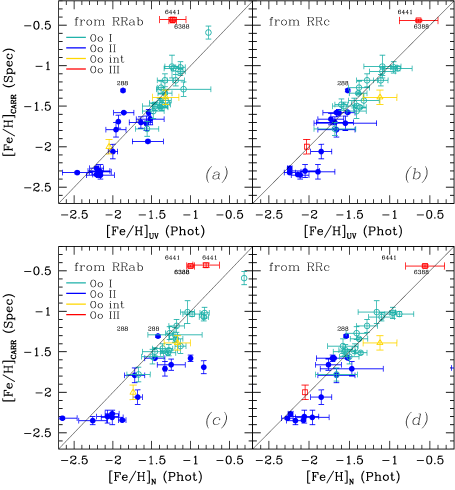
Figure 1: Comparison of the photometric, Fourier decomposition-based [Fe/H]_UV and [Fe/H]_N (Table 1), with equivalent values from high-resolution spectroscopy, [Fe/H]_Carr [13]. (Updated from figure 1 in Arellano Ferro 2022, Rev. Mex. A&A, 58, 257). The color figure can be viewed online.

4.1 Comparison of Fourier [Fe/H] with spectroscopic values

At this point, we would like to compare our photometric calculations of the iron abundances with independent, solidly sustained values. We have chosen to compare with the values given by [13] on the spectroscopic scale [Fe/H]_Carr, for the clusters in Table 1. In Fig. 1, the photometric values [Fe/H]_UV and [Fe/H]_N, obtained as described in the previous section, are plotted versus [Fe/H]_Carr. Given that the results for RRab and RRc stars come from different specific calibrations, the comparison is done separately for both pulsation modes. The top two panels, a and b, show the comparison of [Fe/H]_UV, obtained based on the calibrations of eqs. 2 and 3, duly transformed to the UVES scale. These plots show good agreement between the photometric iron abundance values obtained from the RRab and the RRc stars and the spectroscopic values. There may be a slight hint that the RRc calibration might need a small correction ($\sim-0.2$ dex) for the most metal-poor clusters ([Fe/H]${}_{\rm UV}\leq-1.8$ dex). The bottom two panels, c and d, show the comparison of the values [Fe/H]_N, obtained from the calibrations of [36] (eqs. 4 and 5). For the RRc star, the comparison is satisfactory and comparable to the case in panel b. However, for the RRab stars it is obvious from panel c that the metallicities obtained from eq. 4 are largely overestimated. We do not encourage the use of that calibration for the RRab stars. The same conclusion was reached by Varga et al. in a poster delivered at this IAU Symposium. See also the discussion at the end of the present paper.

4.2 Comparison of Fourier distances with Gaia and HST data based distances

We now proceed to compare the resulting distances from the absolute magnitude determinations resulting from eqs. 6 and 7 described in the previous section. The calculation of the distance involves a value of $E(B-V)$; the adopted values are listed in Table 1. We perform our comparison with accurate critical mean distances from [5], calculated for a large sample of globular clusters using data from Gaia early data release 3 (EDR3) parallaxes, line-of-sight velocity dispersion profiles from Gaia and HST-based proper motions. The top panel of Fig. 2 shows that our distances compare very well with those of BV21. The distance differences are always $<1.9$ kpc and the standard deviation is $0.7$ kpc. The smaller bottom panels show the run of distance differences with [Fe/H]_UV and with the horizontal branch (HB) structural parameter $HBt$. In no case seems there to be a dependence of the distances on either of these quantities.

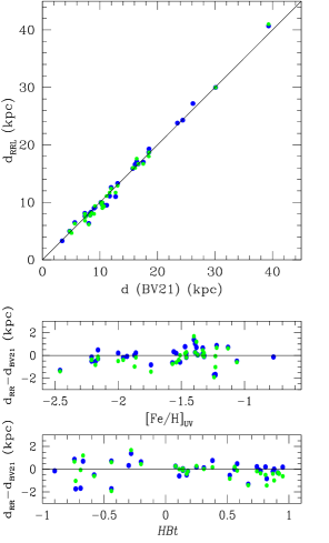
Figure 2: Comparison of distances obtained from the RR Lyrae light curve Fourier decomposition and those of BV21. Blue and green symbols are for distances derived from the calibrations for RRab and RRc, respectively. All distance differences are contained within $\pm 1.9$ kpc of each other and the standard deviation is $0.7$ kpc. (Updated from figure 4 in Arellano Ferro 2022, Rev. Mex. A&A, 58, 257). The color figure can be viewed online.

Individual cluster distances are listed in Table 2. As a complement we have estimated the cluster distances from the P–L relation of SX Phe stars. We have taken into consideration the relations derived by [3] and by [17]. A close look at the table corroborates that these distances are consistent with the determinations from the RR Lyrae stars calculated via the Fourier light curve decomposition.

Table 2: Individual distances for a sample of globular clusters estimated homogeneously from the RR Lyrae stars’ light curve Fourier decompositions and two versions of the SX Phe P–L relation.

GC	$d(kpc)$	$d(kpc)$	$d$ (kpc)	No. of	$d$ (kpc)	$E(B-V)$	d (kpc)
NGC(M)	(RRab)	(RRc)	(SX Phe)	SX Phe	(SX Phe)	mag
			P–L AF11		P–L CS12		BV21
288	9.0$\pm$0.2	8.0	8.8$\pm$0.4	6	9.4$\pm$0.6	0.03	8.988
1261	17.1$\pm$0.4	17.6$\pm$0.7	–	–	–	0.01	16.400
1851	12.6$\pm$0.2	12.4$\pm$0.2	–	–	–	0.02	11.951
1904 (M79)	13.3$\pm$0.4	12.9	–	–	–	0.01	13.078
3201	5.0$\pm$0.2	5.0$\pm$0.1	4.9$\pm$0.3	16	5.2$\pm$0.4	dif	4.737
4147	19.3	18.7$\pm$0.5	–	–	–	0.02	18.535
4590 (M68)	9.9$\pm$0.3	10.0$\pm$0.2	9.8$\pm$0.5	6	–	0.05	10.404
5024 (M53)	18.7$\pm$0.4	18.0$\pm$0.5	18.7$\pm$0.6	13	20.0$\pm$0.8	0.02	18.498
5053	17.0$\pm$0.4	16.7$\pm$0.4	17.1$\pm$1.1	12	17.7$\pm$1.2	0.02	17.537
5272	10.0$\pm$0.2	10.0$\pm$0.4	–	–	–	0.01	10.175
5466	16.6$\pm$0.2	16.0$\pm$0.6	15.4$\pm$1.3	5	16.4$\pm$1.3	0.00	16.120
5904 (M5)	7.6$\pm$0.2	7.5$\pm$0.3	6.7$\pm$0.5	3	7.5$\pm$0.2	0.03	7.479
6139	9.7$\pm$0.7	9.6$\pm$0.6	–	–	–	dif.	10.35
6171	6.5$\pm$0.3	6.3$\pm$0.2	–	–	–	0.33	5.631
6205 (M13)	7.6	6.8$\pm$0.3	7.2$\pm$0.7	4	–	0.02	7.419
6229	30.0$\pm$1.5	30.0$\pm$1.1	27.9	1	28.9	0.01	30.106
6254 (M10)	–	4.7	5.2$\pm$0.3	15	5.6$\pm$0.3	0.25	5.067
6333 (M9)	8.1$\pm$0.2	7.9$\pm$0.3	–	–	–	dif	8.300
6341 (M92)	8.2$\pm$0.2	8.2$\pm$0.4	–	–	–	0.02	8.501
6362	7.8$\pm$0.1	7.7$\pm$0.2	7.1$\pm$0.2	6	7.6$\pm$0.2	0.09	8.300
6366	3.3	–	–	–	–	0.80	3.444
6388	9.5$\pm$1.2	11.1$\pm$1.1	–	–	–	0.40	11.171
6401	6.35$\pm$0.7	6.15$\pm$1.4	–	–	–	dif	8.064
6402 (M14)	9.1$\pm$0.9	9.3$\pm$0.5	–	–	–	0.57	9.144
6441	11.0$\pm$1.8	11.7$\pm$1.0	–	–	–	0.51	12.728
6712	8.1$\pm$0.2	8.0$\pm$0.3	–	–	–	0.35	7.382
6779 (M56)	9.6	9.0		–	–	0.26	10.430
6934	15.9$\pm$0.4	16.0$\pm$0.6	15.8	1	18.0	0.10	15.716
6981 (M72)	16.7$\pm$0.4	16.7$\pm$0.4	16.8$\pm$1.6	3	18.0$\pm$1.0	0.06	16.661
7006	40.7$\pm$1.6	41.0$\pm$1.6	–	–	–	0.08	39.318
7078 (M15)	9.4$\pm$0.4	9.3$\pm$0.6	–	–	–	0.08	10.709
7089 (M2)	11.1$\pm$0.6	11.7$\pm$0.02	–	–	–	0.06	11.693
7099 (M30)	8.32$\pm$0.3	8.1	8.0	1	8.3	0.03	8.458
7492	24.3	–	22.1$\pm$3.2	2	24.1$\pm$3.7	0.00	24.390
Pal2	27.2$\pm$1.8	–	–	–	–	0.93	26.174
Pal 13	23.8$\pm$0.6	–	–	–	–	0.10	23.475

5 The $M_{V}$–[Fe/H] relation

Once we have proven that our photometric determinations of the iron abundances and the absolute magnitudes (hence distances) compare satisfactorily with sound and well-respected independent values, we are in a position to revisit the $M_{V}$–[Fe/H] relation as implied by our results. Before we carry on, let us recall that traditionally, the $M_{V}$–[Fe/H] relation has been considered linear, of the form $M_{V}=\mu$ [Fe/H] + $\gamma$, and that the values of the slope $\mu$ found in the literature range between 0.09 and 0.30 depending on the authors and approach [20, e.g.].

We stress at this point that the values of $M_{V}$ and [Fe/H], obtained from the calibrations for RRab and RRc stars, should not be mixed when displaying the $M_{V}$–[Fe/H] relation since, in doing so, the correlation will turn very noisy and become meaningless, as is obvious from Fig. 3 and the following discussion. In the left panels of Fig. 3, we show the resulting $M_{V}$–[Fe/H] relation based on the results for RRab stars. From top to bottom, panels a, b and c, we display the values of [Fe/H]_ZW, [Fe/H]_UV and [Fe/H]_N, respectively, versus the corresponding $M_{V}$ values from eq. 6. Panel a shows a linear run between [Fe/H]_ZW and $M_{V}$, but the scatter is substantial. Interestingly enough, when [Fe/H]_ZW is converted to the spectroscopic scale, [Fe/H]_UV, panel b, the correlation becomes less dispersed and, most remarkably, it suggests a non-linear trend, very similar in fact to the theoretical predictions of [14] and [45], shown as segmented gray curves in the figure. To the best of our knowledge this is the first empirical $M_{V}$–[Fe/H] relation that follows these theoretical results, at least for RRab results. We will return to this point in the Discussion. In panel c the metallicities from [36] are considered. In this case, and due to the fact noted in Section 4.1 that this calibration overestimates the metallicities, the resulting $M_{V}$–[Fe/H]_N relation turns out to be very scattered and with the RRab results systematically too large.

The quadratic fit in panel b was calculated while excluding the obvious outliers (NGC 288, NGC 7492, M13 based on a single star, and the OoIII type clusters NGC 6388 and NGC 6441), and including M15, and weighing by the number of RRab stars considered in the calculation for each cluster. The correlation is of the form,

$$M_{V}=+0.081(\pm 0.060)\rm[Fe/H]_{\rm UV}^{2}+0.428(\pm 0.207)\rm[Fe/H]_{\rm UV}+1.016(\pm 0.170),$$ (8)

with r.m.s. = 0.060 mag.

Let us turn to the case of the RRc stars, i.e., panels d, e and f on the right of Fig. 3. Now the three panels display linear, tight and very similar correlations. The linear fit in panel e is of the form,

$$M_{V}=0.034(\pm 0.009)\rm[Fe/H]_{\rm UV}+0.601(\pm 0.015),$$ (9)

with r.m.s. = 0.022 mag.

Note that the slope in the above correlation is shallower than the shallowest $M_{V}$–[Fe/H] correlations found in the literature, but it is tight and meaningful. It is also worth to stress that, for the RRc stars, [36]’s calibration is not affected by the bias noticed in their calibration of the RRab stars, and it produces [Fe/H] values that are similar to those of the calibration of [35] (panels d and e).

It shall be obvious now that mixing the RRab and RRc stars in a single $M_{V}$–[Fe/H] relation will lead to a noisy and rather meaningless relation. While this requires some explanation, we shall defer our speculations to the Conclusions.

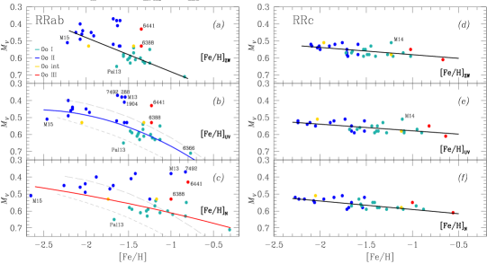
Figure 3: The [Fe/H] versus $M_{V}$ correlations for RRab and RRc stars. The metallicity scales used are, from the top to bottom panels, [Fe/H]_ZW, [Fe/H]_UV and [Fe/H]_N. Cluster type is color coded in the legend in panel (a). All fits have been weighted by the number of RR Lyrae stars included in each cluster. In the panel (b), the gray curves are the theoretical predictions of [14] (long dashes) and [45] (short dashes), which are remarkably similar to the photometric solution. The color figure can be viewed online.

6 The role of the HB structure parameter

In a theoretical study, [20] concluded that the $M_{V}$–[Fe/H] relation is anything but universal, that the slope is also a function of the metallicity range considered, and that for a given metallicity, the luminosity depends on the HB morphology. Following [20], we have adopted the HB type parameter defined as $HBt$ $\equiv(B-R)/(B+V+R)$ [33], where $B,V$ and $R$ are the numbers of HB stars to the blue of the instability strip, RR Lyrae, and those to the red of the instability strip, respectively. We have estimated the value of $HBt$ from the resulting color–magnitude diagrams (CMDs) for almost all clusters in Table 1. Before counting stars we performed a membership analysis using the proper motions, radial velocities and positions available in the different Gaia data releases; [23] and Gaia collaboration (2022) and the membership analysis approach of [11]. For a few clusters for which we have no CMD, we adopted $HBt$ from [43], who also applied membership considerations.

In Fig. 4 the well-known dependence of $HBt$ on metallicity is shown in the left panels for the RRab and the RRc iron abundance solutions. In the right panels, the run of the absolute magnitude $M_{V}$ with $HBt$ is displayed, again separately for the two pulsation modes. The striking feature of these plots is the quadratic correlation between $M_{V}$ and $HBt$ for the RRab solutions, plus the obvious linear correlation of these two quantities for the RRc solutions. The fact that the three parameters [Fe/H]_UV, $M_{V}$ and $HBt$ are interrelated is clear. A multiple regression analysis leads to the following correlations for the RRab and the RRc stars, respectively:

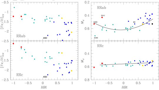
Figure 4: Interdependencies of $M_{V}$, [Fe/H]_UV and the $HBt$ parameter from the solutions for the RRab and the RRc stars. The color figure can be viewed online.

$$M_{V}=A+B\leavevmode\nobreak\ {\rm[Fe/H]}_{\rm UV}+C\leavevmode\nobreak\ {\rm[Fe/H]}_{\rm UV}^{2}+D\leavevmode\nobreak\ {\it HBt}+E\leavevmode\nobreak\ {\it HBt}^{2},$$ (10)

with $A=+1.096(\pm 0.141),B=+0.519(\pm 0.172),C=+0.119(\pm 0.050),D=+0.006(\pm 0.014),E=-0.111(\pm 0.029)$, and r.m.s. = 0.053 mag.

$$M_{V}=+0.609(\pm 0.016)+0.032(\pm 0.009)\leavevmode\nobreak\ \rm[Fe/H]_{\rm UV}+0.015(\pm 0.011)\leavevmode\nobreak\ {\it HBt},$$ (11)

with r.m.s. = 0.024 mag.

We note that in eq. 10 the coefficient $D$ is not significant and that term can therefore be neglected. However, $E$ is significant, hence the quadratic dependence of the calibration on $HBt$ as well as on [Fe/H]_UV. In eq. 11 the coefficient of $HBt$ is not significant, implying a linear correlation between $M_{V}$ and [Fe/H]_UV for the RRc stars’ solutions. If this latter term is ignored, we can see that eqs. 11 and 9 are virtually identical.

The results exposed in this section are in a way the empirical confirmation of the theoretical argumentation of [20], i.e., that a simple linear $M_{V}$–[Fe/H] relation for RR Lyrae in globular clusters is not sufficient but that, for a given metallicity, the luminosity depends on the HB structure, which can be described by the $HBt$ parameter. To this statement we add that this seems indeed the case when the HB luminosities are calculated from RRab stars, whereas the relation remains simple and linear if the luminosity indicators are the overtone RRc stars. If the analysis is performed without distinguishing between both pulsation modes, the presence of RRab stars will contribute to the scatter and non-linearity between $M_{V}$ and [Fe/H]. If RR Lyrae stars are to be used as distance indicators, one should be inclined to prefer the simple RRc stars, and a proper instrument for this purpose could be the $M_{V}$–[Fe/H] relation offered in this work in the form of eq. 9.

7 Variable Stars in our sample of Globular Clusters

The exercise of obtaining accurate photometry in the field of our sample of globular clusters via the DIA, for a time-series of images, as described in Section 2, produces light curves of many point sources in the field of view. Typically between 1000 and 15,000 stars can be isolated and measured, depending on the cluster distance, size, reddening and the prevailing sky conditions during our observations. Exploring all light curves, employing different methods, became a parallel routine in the project. This allowed us to recover the light curves of all known variables and, very often, to find variables not detected previously. The analysis of the light curve shape, period, and the position of the star in the corresponding CMD, generally enables a proper classification of the variable type.

A noteworthy example of the discovery of unexpected variable stars is the case of Palomar 2, well known since a long time as a cluster devoid of variables. However a detailed analysis of our data led to the discovery of 20 RRab stars and 1 RRc. A revision of Gaia DR3 data enabled us to identify 10 additional variables. It has been shown that 16 RRab, 1 RRc and 1 RGB are cluster member stars [2].

Table 3 summarizes the number of variables and their types found during the development of our project. All pertinent details for each cluster, such as their light curves, ephemerides, Fourier fits, classifications and other discussions as to cluster membership and specific peculiarities, can be found in the many original papers referenced and properly coded in table 3 of [1]. The present Table 3 has been updated and edited, and it supersedes table 3 of [1]. In Table 3 we have not included any variable star listed as such in the Gaia DR3 in the corresponding field of each cluster. Many of the Gaia variables coincide with previously known variables and/or may be field stars. Therefore, while we are not aware of a dedicated analysis of these variables, as for example for the case of Palomar 2 [2] or NGC 6139 (Yepez et al. 2023), we have based our star counts on the present edition of the Catalog of Variable Stars in Globular Clusters [15] and our own findings.

Table 3: Number of presently known variables per type and per cluster for the most common variable types, in the globular clusters studied by our group$\dagger$.

GC	RRab	RRc	RRd	SX Phe	Binaries	CW-(AC)-RV	SR, L, M	unclass	Total per cluster
NGC (M)								others $*$
288	0/1	0/1	0/0	0/6	0/1	0/0	0/1	–	0/10
1261	0/16	0/6	0/0	0/3	0/1	0/0	0/3	–	0/29
1904 (M79)	0/6	1/5	0/0	0/5	0/1	0/1	0/14	0/1	1/32
3201	0/72	0/7	0/0	3/24	0/11	0/0	0/8	0/7	3/122
4147	0/5	0/19	0/1	0/0	0/14	0/0	2/2	0/3	2/41
4590 (M68)	0/14	0/16	0/12	4/6	0/0	0/0	0/0	1/2	4/48
5024 (M53)	0/29	2/35	0/0	13/28	0/0	0/0	1/12	–	16/104
5053	0/6	0/4	0/0	0/5	0/0	0/0	0/0	–	0/15
5466	0/13	0/8	0/0	0/9	0/3	0/1	0/0	2/2	0/34
5904 (M5)	2/ 89	1/40	0/0	1/6	1/3	0/2	11/12	0/1	16/152
6171 (M107)	0/15	0/6	0/0	0/1	0/0	0/0	2/3	0/3	2/25
6139	0/4	4/5	0/0	0/0	1/1	0/0	4/7		9/17
6205 (M13)	0/1	1/7	2/2	2/6	1/3	0/3	3/22	0/4	9/44
6229	10/42	5/15	0/0	1/1	0/0	2/5	6/6	0/1	24/69
6254 (M10)	0/0	0/1	0/0	1/15	2/10	0/3	0/5	0/2	3/34
6333 (M9)	0/8	2/10	1/1	0/0	3/4	1/1	5/6	3/4	12/30
6341 (M92)	0/9	0/5	1/1	1/6	0/0	0/1	1/1	0/6	3/23
6362	0/16	0/15	1/3	0/6	0/12	0/0	0/0	0/22	1/52
6366	0/1	0/0	0/0	1/1	1/1	1/1	3/4	–	6/8
6388	1/14	2/23	0/0	0/1	0/10	1/11	42/58	–	46/117
6397	0/0	0/0	0/0	0/5	0/15	0/0	0/1	0/13	0/21
6401	6/23	6/11	0/0	0/0	0/14	0/1	3/3	14/14	15/52
6402 (M14)	0/55	3/56	1/1	1/1	0/3	0/6	18/32		23/154
6441	2/50	0/28	0/1	0/0	0/17	2/9	43/82	0/10	47/187
6528	1/1	1/1	0/0	0/0	1/1	0/0	4/4	–	7/7
6638	3/10	2/18	0/0	0/0	0/0	0/0	3/9	0/25	8/37
6652	0/3	0/1	0/0	0/0	1/2	0/1	0/2	1/5	1/9
6712	0/10	0/4	0/0	0/0	2/2	0/0	5/11	0/8	7/27
6779 (M56)	0/1	0/2	0/0	1/1	3/3	0/2	0/3	1/6	4/12
6934	3/68	0/12	0/0	3/4	0/0	2/3	3/5	1/6	11/92
6981 (M72)	8/37	3/7	0/0	3/3	0/0	0/0	0/1		14/48
7078 (M15)	0/65	0/67	0/32	0/4	0/3	0/2	0/3	0/11	0/176
7089 (M2)	5/23	3/15	0/0	0/2	0/0	0/4	0/0	0/12	8/44
7099 (M30)	1/4	2/2	0/0	2/2	1/6	0/0	0/0	0/3	6/14
7492	0/1	0/2	0/0	2/2	0/0	0/0	1/2	–	3/7
Pal 2	16/16	1/1	0/0	0/0	0/0	0/0	1/1	–	18/18
Pal 13	0/4	0/0	0/0	0/0	0/0	0/0	1/1		1/5
Total per type	58/732	41/454	6/54	39/153	17/141	9/57	162/324	23/171 *	330/1916

$\dagger$. The variable star types have been adopted from the General Catalog of Variable Stars [26, 38]. Entries expressed as $M/N$ indicate the $M$ variables found or reclassified by our program and the total number $N$ of presently known variables. Relevant papers on individual clusters can be found properly coded in table 3 of [1].

$*$. Numbers from this column are not considered in the totals, since they include unclassified or likely field variables.

8 Summary and Conclusions

For nearly two decades, systematic observational scrutiny of the variable star populations in a sample of 39 globular clusters by means of time-series CCD imaging in the VI passbands, and their treatment by the DIA, enabled to collect numerous light curves of variable stars, of many types, contained in these stellar systems. Of particular interest to the present work were the light curves of RR Lyrae stars of both pulsation modes, the fundamental RRab and the first overtone RRc groups. We have performed Fourier decompositions of these light curves and the resulting Fourier parameters have been employed in carefully selected empirical calibrations to calculate, in an unprecedentedly homogeneous manner, the atmospheric iron abundances, [Fe/H], and absolute magnitudess, $M_{V}$, via this photometric approach. Attention was paid to the zero points of the absolute magnitude calibrations.

The mean $M_{V}$ values and estimates of the interstellar reddening led to photometric distances calculated for our sample 39 globular clusters and reported here. The mean iron abundance for a given cluster was calculated on the scale of [47] [Fe/H]_ZW, transformed to the UVES spectroscopic scale of [13] [Fe/H]_UV, and on the scale of [36] [Fe/H]_N.

The photometric [Fe/H]_UV and the spectroscopic [Fe/H]_CARR values taken from [13] were found to be in very good agreement for both the solutions from the RRab and the RRc stars. [36]’s calibration for the RRc stars are also in good agreement with both [Fe/H]_UV and [Fe/H]_CARR. It was found, however, that the photometric values from the calibration for RRab stars of [36] are systematically overestimated relative to the spectroscopic values. This result becomes of particular relevance since the calibration of [36] was used by Gaia to calculate the iron abundances from the photometry of RR Lyrae stars. It is worth noting that a similar result has been reported in a poster presented at this meeting by Varga et al. See also the Q&A section below for further comments on this issue.

Similarly, we have compared our photometric determinations of the accurate mean cluster distances derived by [5]. The agreement is outstanding, yielding distance differences within $\pm 1.9$ kpc for the entire distance range up to 40 kpc.

The resulting $M_{V}$–[Fe/H] relation for the RRab stars looks non-linear and scattered. However, based on the RRc stars the relation remains linear and tight. The latter relation shows only a mild but significant dependence of the luminosity on the metallicity. It is clear that if the $M_{V}$ and [Fe/H] results from RRab and RRc stars are mixed, the resulting $M_{V}$–[Fe/H] relation will be apparently linear, very scattered and steeper. We find that it is important to segregate the RRab and RRc results for a more meaningful interpretation of the $M_{V}$–[Fe/H] relation.

As suggested on theoretical grounds [20], we have empirically shown that the HB type parameter, $HBt$, plays a significant role in the $M_{V}$–[Fe/H] relation if calculated using the RRab stars as tracers, in which case the relation becomes quadratic in [Fe/H] and $HBt$. No dependence on $HBt$ was found for the RRc stars. These results strengthen the notion that RRc stars may be more trusted distance indicators than their more complex RRab counterparts.

While I really do not have an in-depth explanation for the differences in the luminosity dependence on the metallicity for RRab and from RRc stars, it may be relevant to mention that RRab stars carry a greater degree of complexity; they have larger amplitudes, many of them have (undetected) Blazhko modulations, their light curves are asymmetrical and hence prone to more inaccurate Fourier decompositions; as their periods are often longer, their light curves are not fully or rather unevenly covered. Their evolutionary tracks toward the RGB are spread more widely with small variations in age, inner mass structure and chemical differences. The RRc stars, on the other hand, are simpler, easier to decompose and their luminosities are less sensitive to age, mass or chemistry. However I emphasize that the remarks in the present work may require further theoretical input.

Systematic time-series CCD imaging and differential image analysis performed over the last nearly 20 years has enabled us to report and classify 330 newly detected variables in our sample of globular clusters.

9 Acknowledgments

I am indebted to all my friends and colleagues who have accompanied me on this globular cluster journey that has lasted nearly two decades. They number too many to specifically name them all here; their names are all included as co-authors of our papers; to all of them, my gratitude for having shared with me and taught me their expertise. I am particularly thankful to the Time Allocation Committees of several observatories for having generously granted the time needed to push forward our observing strategies. For many years, the project has received support from the Institute of Astronomy and DGAPA, of the National Autonomous University of Mexico, through a range of grant numbers.

Questions and Answers

Clara Martínez-Vázquez: Thanks for your talk and the interesting comments offered! I would like to bring to your attention a set of recently published new $P$–$\phi_{31}$–[Fe/H] relationships for RRab and RRc types. They have been calibrated based on a very large and homogeneous sample of spectroscopic metallicities. The testing of the relations has proven to be very efficient. Here are the papers in case you want to check them: https://iopscience.iop.org/article/10.3847/1538-4357/abefd4 ($P$–$\phi_{31}$–[Fe/H] for RRab) and https://iopscience.iop.org/article/10.3847/1538-4357/ac67ee ($P$–$\phi_{31}$–[Fe/H] for RRc).

AAF: Thank you so much for the references. I will check them carefully.

Héctor Vázquez Ramló: Thanks for the interesting talk. A technical question: if I understood you correctly, you use differential imaging to obtain the light curves of the RR Lyrae in globular clusters. That implies soundly coping with PSF variations from image to image (at least if observations were obtained from the ground, I didn’t get if that is the case). Could you expand a little on this, please? Which package do you use?

AAF: We use Difference Image Analysis (DIA) through the pipeline DanDIA (Bramich 2008, MNRAS, 386, L77; Bramich et al. 2013 MNRAS, 428, 2275). DanDIA is constructed based on the DanIDL library of IDL routines available at http://www.danidl.co.uk. Our use is described in detail in Bramich et al. (2011 MNRAS, 413, 1275). A recent paper where you can gain an overall view of all our procedures is perhaps Yepez et al. (2020, MNRAS, 494, 3212). Regarding the PSF, DanDIA constructs a reference image from a combination of the best images in our collection. Then, it isolates up to 400 stars in the image using some isolation criteria, and it uses those individual PSFs to search for possible trends across the chip, fitting high-order polynomials. The PSF kernel is then used for the individual differential images.

Héctor Vázquez Ramló: Another question regarding the statement of RRc being more suitable for distance measurements, that was an interesting one. It is clear that RRab are more widely used due to their much higher abundance and their higher pulsation amplitude (easier to identify) in comparison with RRc. Out of curiosity, I really don’t know: are there studies exclusively focusing on RRc for estimating distances? Is there a general consensus in the community on that issue?

AAF: There are of course papers dedicated exclusively to RRc stars, for instance one on spectral metallicity determinations by Sneden et al., (2018, AJ, 155, 45), but not on the premise that they may be better distance indicators, I think. This is, in fact, one of the highlights among our results; this, and the fact that absolute magnitudes of mixed samples of RRab and RRc stars will lead to larger uncertainties and mislead calibrations of the famous $M_{V}$–[Fe/H] correlation. I do not think there is, at present, a general consensus on these points, or not just yet. The community has become more interested in the presence of secondary frequencies caused by non-radial modes in RRc stars, I believe, the ones with ratios relative to the overtone frequency ($f_{1}$) known as the $f_{61}/f_{1}\sim 0.61$–$0.65$.

Gergely Hajdu: Thank you very much for the update on globular cluster RR Lyrae. I would like to discourage the use of the Nemec et al. (2013) relations for metallicity estimation of RRab stars. They come from a very small sample of variables, and the authors overfit their data with parameters that are highly correlated (especially their three parameters that all contain $\phi_{31}$), as shown by the large formal errors (4.64 dex on the intercept!). Unfortunately, the baseline Gaia DR3 [Fe/H] estimates are based on this formula, leading to clearly artificial features appearing when the Bailey diagram is colored according to that metallicity estimate (i.e., fig. 35 of https://ui.adsabs.harvard.edu/abs/2022arXiv220606278C/abstract).

AAF: Thanks for your comments. As you may have noticed, in our comparison of the photometric estimates of [Fe/H]_UV vs. the spectroscopic values, [Fe/H]_CARR, we also noticed that something does not work well for the calibration of Nemec et al. (2013) for the RRab stars, since their calibration clearly overestimates the iron abundance values. For the RRc stars, it seems as good as the calibration of Morgan et al. (2007). Thus, it is interesting to note your comments and recommendation against that calibration. By the way, there is a poster at this Symposium by Varga et al.; the authors reached the same conclusion as regards Nemec et al.’s calibration for the RRab and, apparently, they have corrected it.

Vázsony Varga: I also recommend comparision with Fabrizio et al.’s (2021) $\Delta S$ Bailey diagram metallicity distribution. I’d also like to add that the anomalous metal-rich regions in the current Gaia Bailey diagram are likely caused by the small parameter space covered by the calibration data set.

AAF: Thank you for your comments. I have noticed that you also highlight that the calibration of [36] overestimates the iron abundances for RRab stars.

References

- [1] A. Arellano Ferro “A Vindication of the RR Lyrae Fourier Light Curve Decomposition for the Calculation of Metallicity and Distance in Globular Clusters” In Rev. Mexicana Astron. Astrofis. 58, 2022, pp. 257–271 DOI: 10.22201/ia.01851101p.2022.58.02.08
- [2] A. Arellano Ferro, I. Bustos Fierro, S. Muneer and S. Giridhar “RR Lyrae Stars in the Globular Cluster Palomar 2” In Rev. Mexicana Astron. Astrofis. 59, 2023, pp. 3–10 DOI: 10.22201/ia.01851101p.2023.59.01.01
- [3] A. Arellano Ferro et al. In MNRAS 416, 2011, pp. 2265
- [4] A. Arellano Ferro, Sunetra Giridhar and D.. Bramich “CCD time-series photometry of the globular cluster NGC 5053: RR Lyrae, Blue Stragglers and SX Phoenicis stars revisited” In MNRAS 402, 2010, pp. 226–244
- [5] H. Baumgardt and E. Vasiliev “Accurate distances to Galactic globular clusters through a combination of Gaia EDR3, HST, and literature data” In MNRAS 505.4, 2021, pp. 5957–5977 DOI: 10.1093/mnras/stab1474
- [6] G. Benedict et al. “Astrometry with the Hubble Space Telescope: A Parallax of the Fundamental Distance Calibrator RR Lyrae” In AJ 123.1, 2002, pp. 473–484 DOI: 10.1086/338087
- [7] D.. Bramich “A new algorithm for difference image analysis” In MNRAS 386, 2008, pp. L77–L81 arXiv:0802.1273
- [8] D.. Bramich et al. “Difference image analysis: The interplay between the photometric scale factor and systematic photometric errors” In A&A 577, 2015, pp. A108 DOI: 10.1051/0004-6361/201526025
- [9] D.. Bramich, R. Figuera Jaimes, Sunetra Giridhar and A. Arellano Ferro “CCD time-series photometry of the globular cluster NGC 6981: variable star census and physical parameter estimates” In MNRAS 413.2, 2011, pp. 1275–1294
- [10] D.. Bramich et al. “Difference image analysis: extension to a spatially varying photometric scale factor and other considerations” In MNRAS 428, 2013, pp. 2275–2289
- [11] Iván H. Bustos Fierro and J.. Calderón “Extraction of globular clusters members with Gaia DR2 astrometry” In MNRAS 488, 2019, pp. 3024
- [12] C. Cacciari, T.. Corwin and B.. Carney “A Multicolor and Fourier Study of RR Lyrae Variables in the Globular Cluster NGC 5272 (M3)” In AJ 129.1, 2005, pp. 267–302 DOI: 10.1086/426325
- [13] E. Carretta et al. “Intrinsic iron spread and a new metallicity scale for globular clusters” In A&A 508, 2009, pp. 695–706 arXiv:0910.0675
- [14] S. Cassisi et al. “Galactic globular cluster stars: From theory to observation” In A&AS 134, 1999, pp. 103–113 DOI: 10.1051/aas:1999126
- [15] Christine M. Clement et al. “Variable Stars in Galactic Globular Clusters” In AJ 122.5, 2001, pp. 2587–2599 DOI: 10.1086/323719
- [16] Gisella Clementini et al. “Distance to the Large Magellanic Cloud: The RR Lyrae Stars” In AJ 125.3, 2003, pp. 1309–1329 DOI: 10.1086/367773
- [17] R.. Cohen and A. Sarajedini In MNRAS 419, 2012, pp. 342
- [18] R. Contreras et al. “Time-series Photometry of Globular Clusters: M62 (NGC 6266), the Most RR Lyrae-rich Globular Cluster in the Galaxy?” In AJ 140.6, 2010, pp. 1766–1786 DOI: 10.1088/0004-6256/140/6/1766
- [19] Richard de Grijs, James E. Wicker and Giuseppe Bono “Clustering of Local Group Distances: Publication Bias or Correlated Measurements? I. The Large Magellanic Cloud” In AJ 147.5, 2014, pp. 122 DOI: 10.1088/0004-6256/147/5/122
- [20] Pierre Demarque, Robert Zinn, Young-Wook Lee and Sukyoung Yi “The Metallicity Dependence of RR Lyrae Absolute Magnitudes from Synthetic Horizontal-Branch Models” In AJ 119.3, 2000, pp. 1398–1404 DOI: 10.1086/301261
- [21] D. Deras et al. “A new study of the variable star population in the Hercules globular cluster (M13; NGC 6205)” In MNRAS 486.2, 2019, pp. 2791–2808 DOI: 10.1093/mnras/stz642
- [22] Wendy L. Freedman et al. “Final Results from the Hubble Space Telescope Key Project to Measure the Hubble Constant” In ApJ 553.1, 2001, pp. 47–72 DOI: 10.1086/320638
- [23] Gaia Collaboration et al. “The Gaia mission” In A&A 595, 2016, pp. A1 DOI: 10.1051/0004-6361/201629272
- [24] J. Jurcsik “Revision of the [Fe/H] Scales Used for Globular Clusters and RR Lyrae Variables” In Acta Astron. 45, 1995, pp. 653–660
- [25] J. Jurcsik and G. Kovács “Determination of [Fe/H] from the light curves of RR Lyrae stars.” In A&A 312, 1996, pp. 111–120
- [26] E.. Kazarovets et al. “A Catalog of Variable Stars based on the new name list” In Astronomy Reports 53.11, 2009, pp. 1013–1019 DOI: 10.1134/S1063772909110067
- [27] T.. Kinman “The Absolute Magnitude (M_v) of Type ab RR Lyrae Stars” In Information Bulletin on Variable Stars 5354, 2002, pp. 1
- [28] G. Kovács “Relative distance moduli based on the light and color curves of RR Lyrae stars.” In Mem. Soc. Astron. Italiana 69, 1998, pp. 49–57
- [29] G. Kovács and S.. Kanbur “Modelling RR Lyrae pulsation: mission (im)possible?” In MNRAS 295.4, 1998, pp. 834–846 DOI: 10.1046/j.1365-8711.1998.01271.x
- [30] G. Kovács and A.. Walker “Empirical relations for cluster RR Lyrae stars revisited” In A&A 374, 2001, pp. 264
- [31] G. Kovács and E. Zsoldos “A new method for the determination of [Fe/H] in RR Lyrae stars.” In A&A 293, 1995, pp. L57–L60
- [32] Andrew C. Layden “The Metallicities and Kinematics of RR Lyrae Variables. I. New Observations of Local Stars” In AJ 108, 1994, pp. 1016 DOI: 10.1086/117132
- [33] Young-Wook Lee, Pierre Demarque and Robert Zinn “The Horizontal-Branch Stars in Globular Clusters. II. The Second Parameter Phenomenon” In ApJ 423, 1994, pp. 248 DOI: 10.1086/173803
- [34] J. Lub “An atlas of light and colour curves of field RR Lyrae stars.” In A&AS 29, 1977, pp. 345–378
- [35] Siobahn M. Morgan, Jennifer N. Wahl and Rachel M. Wieckhorst “[Fe/H] relations for c-type RR Lyrae variables based upon Fourier coefficients” In MNRAS 374.4, 2007, pp. 1421–1426
- [36] James M. Nemec et al. “Metal Abundances, Radial Velocities, and Other Physical Characteristics for the RR Lyrae Stars in The Kepler Field” In ApJ 773.2, 2013, pp. 181
- [37] G. Pietrzyński et al. “An eclipsing-binary distance to the Large Magellanic Cloud accurate to two per cent” In Nature 495.7439, 2013, pp. 76–79 DOI: 10.1038/nature11878
- [38] N.. Samus et al. “A Catalog of Accurate Equatorial Coordinates for Variable Stars in Globular Clusters” In PASP 121.886, 2009, pp. 1378 DOI: 10.1086/649432
- [39] Norman R. Simon “On Metallicity and RR Lyrae Light Curves” In ApJ 328, 1988, pp. 747 DOI: 10.1086/166333
- [40] Norman R. Simon “The Fourier Decomposition Technique: Interpreting the Variations of Pulsating Stars” In Pulsation and Mass Loss in Stars 148, Astrophysics and Space Science Library, 1988, pp. 27 DOI: 10.1007/978-94-009-3029-2˙2
- [41] Norman R. Simon and Christine M. Clement “A Provisional RR Lyrae Distance Scale” In ApJ 410, 1993, pp. 526 DOI: 10.1086/172771
- [42] Nicholas B. Suntzeff, Robert P. Kraft and T.. Kinman “Summary of Delta S Metallicity Measurements for Bright RR Lyrae Variables Observed at Lick Observatory and KPNO between 1972 and 1987” In ApJS 93, 1994, pp. 271 DOI: 10.1086/192055
- [43] M. Torelli et al. “Horizontal branch morphology: A new photometric parametrization” In A&A 629, 2019, pp. A53 DOI: 10.1051/0004-6361/201935995
- [44] T.. Van Albada and N. Baker “On the Masses, Luminosities, and Compositions of Horizontal-Branch Stars” In ApJ 169, 1971, pp. 311
- [45] Don A. VandenBerg et al. “Models for Old, Metal-poor Stars with Enhanced -Element Abundances. I. Evolutionary Tracks and ZAHB Loci; Observational Constraints” In ApJ 532.1, 2000, pp. 430–452 DOI: 10.1086/308544
- [46] M.. Yepez, A. Arellano Ferro and D. Deras “CCD VI time-series of the extremely metal-poor globular cluster M92: revisiting its variable star population” In MNRAS 494.3, 2020, pp. 3212–3226
- [47] R. Zinn and M.. West “The globular cluster system of the galaxy. III - Measurements of radial velocity and metallicity for 60 clusters and a compilation of metallicities for 121 clusters” In ApJS 55, 1984, pp. 45–66