Large Master Field Optimization: the Quantum Mechanics of two Yang-Mills coupled Matrices
Abstract
We study the large dynamics of two massless Yang-Mills coupled matrix quantum mechanics, by minimization of a loop truncated Jevicki-Sakita effective collective field Hamiltonian. The loop space constraints are handled by the use of master variables. The method is successfully applied directly in the massless limit for a range of values of the Yang-Mills coupling constant, and the scaling behaviour of different physical quantities derived from their dimensions are obtained with a high level of precision. We consider both planar properties of the theory, such as the large ground state energy and multi-matrix correlator expectation values, and also the spectrum of the theory. For the spectrum, we establish that the traced fundamental constituents remain massless and decoupled from other states, and that bound states develop well defined mass gaps, with the mass of the two degenerate lowest lying bound states being determined with a particularly high degree of accuracy. In order to confirm, numerically, the physical interpretation of the spectrum properties of the traced constituents, we add masses to the system and show that, indeed, the traced fundamental constituents retain their ”bare masses”. For this system, we draw comparisons with planar results available in the literature.
1 Introduction
Multi-matrix systems 111We have in mind the path integral or the quantum mechanics of a finite number of matrices. are important in many different physical settings, not only as of finite sized matrices, but particularly in their large limit [1]. They are expected to provide a reduced ansatz for large gauge theories, both in the path integral [2, 3, 4, 5, 6] and Hamiltonian formulations [7, 8], and both for unitary as well as hermitian matrices. Their interpretation as branes [9] has led to the suggestion that they may provide a definition of M theory[10], also argued to be valid for the path integral [11]. The correspondence [12, 13, 14] has highlighted the importance of SYM theory, with its bosonic adjoint scalar sector, and ensuing integrability properties [15] and Hamiltonian reductions [16], [17, 18, 19]. They are used in the study of black holes [20, 21, 22]222There is a vast literature on matrix models; we have tried to highlight only some key developments in their application, with emphasis on YM coupled systems..
We study in this communication the large properties of the Hamiltonian of two massless matrices interacting via a Yang-Mills potential. We are able to study the system directly in the large limit and directly in the massless limit. In general [23, 24], properties of the massless system are obtained by extrapolation of a system with a finite mass parameter to zero. In our case, being able to work directly with the massless system, we are able to obtain the asymptotic scaling behaviour of physical quantities and correlators, and determine their parameters, with a high degree of accuracy.
In addition to its interpretation as a reduced model, or bosonic scalar subsector of SYM, this Hamiltonian has associated with it a number of puzzles, mainly around the properties of its spectrum and of the presence or not of a mass gap [25, 26, 27]. Within the context of the expansion, we provide a definite answer to this question in this article.
Our approach is based on the collective field theory Hamiltonian of Jevicki and Sakita [28]. This Hamiltonian is an exact re-writing of a given theory in terms of its (gauge) invariant variables. The large (planar) background is then obtained semiclassically as the minimum of an effective potential and, when expanded about this large background, the collective field theory Hamiltonian generates corrections systematically 333For a single matrix based example, see for instance [29], [30]. Also, although we consider matrix valued systems in this communication, the same is true of vector valued field theories..
The idea behind the method is to implement a change of variables from the original variables of the theory, generically denoted by , to the invariant set of operators (the collective fields), generically denoted by , and to require explicit hermiticity of the collective field Hamiltonian. This change of variable is accompanied by a Jacobian . In general is not known explicitly, but it satisfies the following equation
This is sufficient to obtain explicitly the collective field Hamiltonian in terms of and its canonical conjugate . In general,
joins two loops into a sum of single loops444The terminology ”loop” is inherited from gauge theories, where the gauge invariant variables are Wilson loops. But in this communication they refer to operators that are invariant under the gauge symmetries allowed by the system under consideration., and splits a given loop into a sum of two (in general smaller) loops. Details of their form will be given in the following.
The collective field Hamiltonian is ideally suited to a numerical approach based on minimisation of the effective potential , in a truncated loop space that can be systematically increased and ascertained for convergence and accuracy. Indeed, already some time ago [31, 32], this approach was successfully implemented in the context of lattice gauge theories with Wilson’s one-plaquette action [33]. Systems of unitary matrices have a phase transition between a strong and weak phase, and it was established in [31, 32] that in the weak coupling phase the minimization has to be accompanied by a constraint:
| (1) |
In other words, the large expectation values of the loop variables must satisfy the constraint that the matrix is semi-positive definite, with a number of eigenvalues saturating to zero in the weak coupling regime. This was shown to also be the case when considering loop equations [34].
This constraint is not difficult to understand: the large limit of the single unitary matrix integral has a well known third order phase transition [35], described in terms of the density of its (phases of) eigenvalues as:
| (2) |
In the strong coupling regime, the density of eigenvalues is periodic with period . For weak coupling, the density of eigenvalues develops finite support within the interval , and outside this finite support.
A similar phase transition and pattern in the density of eigenvalues is present in the large limit of the quantum mechanics of single unitary matrix systems [36, 37, 38, 39]. Systems of hermitian matrices have only one single (weak) phase, so ensuring that outside their finite support in order that the density of states remains non-negative is of paramount importance.
For a single hermitian matrix , with invariants , the density of eigenvalues is simply its Fourier transform, . Then:
So, in this simple case, is seen to have zero eigenvalues when the density matrix has zero eigenvalues, or when . For single matrix systems then, this constraint on is easily related to the requirement that the density is non-negative.
In the case of more complex multi-matrix systems, and in the context of the collective field theory approach, the required constraint is then that the loop space matrix
is semi-positive definite. This follows from the definition of , on the left hand side of the above equation, but no longer apparent once is expressed in terms of loop variables, as on the right hand side of the above equation. The semi-positiveness condition results in a number of inequalities amongst the loop variables. These are the non-linear constraints that large expectation values of invariant operators have to satisfy, some of which are saturated. For instance, if the ’s are hermitian matrices, the operation acting on a single trace loop of a product of these matrices removes everywhere where it is present along the loop and ”opens up an open string”. can then be thought of as a matrix of (linear combinations of) open string inner products, linking to the interpretation as suggested in [40]. 555For a unitary matrices, .
Interest in the development of numerical techniques applicable directly to the large limit properties of multi matrix systems has been rekindled recently [40, 41, 42, 43, 44], and the importance the loop space constraints re-discovered [40, 41, 42, 43], in a program generically referred to as numerical bootstrap. In [40, 43, 45] the constrained optimisation problem uses semidefinite programming in solving loop equations directly in loop space. In [41], the loop equations are iterated and a set of small loops adjusted to satisfy the constraints, and this method is generalized to matrix quantum mechanics in [42], where some exact bounds are also obtained.
In this article we carry out a numerical study of the large limit of the quantum mechanics of two hermitian matrices coupled by a Yang-Mills potential using a truncated collective field Hamiltonian. We are able to carry out this study directly in the massless limit, with the different loop quantities considered exhibiting the expected scaling properties with an extremely high degree of accuracy. As indicated earlier, since the collective hamiltonian is an exact loop space re-writing of the large theory, it has a systematic expansion. In particular then, and as a quantum mechanical system, we are able to study its mass spectrum in addition to the planar properties of the theory. The study of the spectrum and ensuing absence or presence of mass gaps is of particular importance to matrix gauge theories. We believe that currently, this is the only method able to provide information about the large spectrum of the theory.
The issue of constraints is addressed by the use of ”master variables” [32, 44, 46]. These are variables that satisfy the constraints explicitly, of which the original variables are an example. In addition to satisfying the constraints in the planar limit, they can be used to set up the spectrum equations of the theory [46]. For two matrix systems, we keep one of the matrices diagonal and the other as an arbitrary hermitian, so that there are master variables.
The fact that another parameter has been introduced in addition to the truncation parameter may seem undesirable. But the extensive study of two matrix hamiltonians with cubic, quartic and mixed quadratic potential carried in [44] as well as further evidence provided in this article establish the stability and accuracy of this approach666It also opens the possibility of direct studies of stringy (gravity and brane) phenomena emerging from properties of single trace operators of length related to different powers of , as embedded in the AdS/CFT correspondence [12, 13, 14],[16],[48]. This is beyond the scope of this communication. .
Loop equations of the integral correspond to the statement of minimization of the large loop collective effective potential of a suitably defined quantum mechanical Hamiltonian, namely the Fokker-Planck Hamiltonian [34] 777This effective potential also gives the leading Large loop configuration of the bosonic sector of supersymmetric multi matrix Marinari-Parisi [49] type models [50],[51] .. This is the best way to understand that constraints, (which in the collective field approach are encapsulated in the statement that ) arise even in the context of loop equations [34], and as argued differently and more recently in [40]. An extensive study of two matrix loop equations with cubic, quartic and mixed quadratic potential was carried in [44], which were shown to be satisfied to a very high level of accuracy. In this article, however, we are interested in the matrix quantum mechanics Hamiltonian of two Yang-Mills coupled matrices.
This article is organized as follows: after the current Introduction, Section describes the method, the loop truncation and the use of master variables in dealing with the loop space constraints. Their use in obtaining both the large loop background, and concomitant planar quantities, as well as the spectrum, is described. In Section we apply the method to the large limit of the quantum mechanics of two Yang-Mills coupled, massless matrices. We find that the method displays perfect stable convergence directly in this massless limit. Moreover, physical quantities exhibit the scaling behaviour determined by their dimensions with a very high level of accuracy, both for planar quantities and for the spectrum. In other words, the loop truncated collective field Hamiltonian is entirely consistent with the scaling properties of the full massless theory. Only correlators of zero charge of the symmetry of the system are shown to develop non-zero planar expectation values, and we assign charges to spectrum states. For the spectrum, we argue that the two lowest states, the traced constituent single particle states 888These are absent for ., are numerically massless, and associate them with the non-interacting subgroup of the system. Higher energy (bound) states develop well defined mass-gaps. In order to confirm our physical interpretation of the two lowest degenerate states as massless states, we add masses to the system in Section , where it is verified indeed that their ”bare mass” is not corrected. Mass corrected fits to the planar ground state energy, to the first few bound states and to planar correlators are presented, some of which are compared with (the few results available in) the literature. As for the massless case, it is confirmed that only zero charge correlators develop non-zero expectation values, and charges to spectrum states are assigned. Section is left for a conclusion and future outlook. The Appendix discusses estimates of errors in our numerical method.
2 Method, loop truncation and master variables
We consider the quantum mechanics of two hermitian matrices , interacting via a Yang-Mills potential:
is canonical conjugate to , and is a mass. The massless case will be considered first in Section 3 and the massive case in Section 4. Note that in terms of our conventions, ’t Hooft’s coupling is .
The invariant loops are single traces of products of the matrices , up to cyclic permutations:
For instance, with two matrices one has , with three matrices , etc., with an obvious notation. We will continue to refer to the invariant variables as “loops”, for the historical reasons explained in the introduction.
The collective field Hamiltonian [28] in terms of the invariant loops takes the form
where is the canonical conjugate to , and
If has length (number of matrices in the loop) and has length , joins them into a number of loops of length . splits the loop of length into sets of two loops and with total lengths . contains subleading counterterms that need not be considered for the large N background and the spectrum.
We then consider
In order to exhibit explicitly the large dependence, we let
and obtain
| (3) | ||||
| (4) |
It follows that the large background is the minimum of subject to the constraint that is semi-positive definite.999The discussion next in this section follows closely that of [44], which is based on [31, 32, 46].
2.1 Truncation of loop space
For a given (), is truncated to be a matrix, where is the number of loops of length or less. itself, however, depends on loops with lengths up to . If is the number of loops with length or less, then it is seen that in (4) is a function of :
These parameters are listed in the following table for different levels of truncation.
| 4 | 9 | 15 |
| 6 | 15 | 37 |
| 8 | 23 | 93 |
| 10 | 37 | 261 |
| 12 | 57 | 801 |
| 14 | 93 | 2615 |
| 16 | 153 | 8923 |
| 18 | 261 | 31237 |
2.2 Master fields and planar limit.
In order to minimize subject to the constraint , we introduce master variables that explicitly satisfy the constraint:
Specifically, we choose to be diagonal and an arbitrary hermitian matrix. The master field then has real components
The planar limit is obtained by minimizing with respect to the master variables. More precisely, at the minimum,
| (5) | ||||
| (6) |
In general, . The planar background is specified by the large expectation values of all gauge invariant operators.
Details of the numerical algorithm have been given in [44]. In this article, we have chosen a truncation with , that is, and a matrix. For the master field, we took , corresponding to master variables. Evidence for the consistency of the truncation and stability with respect to different values of has been provided in [44], and is also presented in Appendix A for the Yang-Mills coupled systems considered in this communication.
2.3 Spectrum and master variables
It is important to keep in mind that the expansion is an expansion in terms of loop variables. As such, letting
we expand (3) up to second order:
But
and hence the term linear in in vanishes, as a result of (5).
It is important to note that is not the same as . is a matrix ( evaluated at the minimum of ), but is a matrix! In practice, it cannot be calculated in loop space as a loop joining matrix; it would require generating all loops with length or less101010For the truncated system with , one would have to identify loops containing up to matrices.. However, at the minimum, it can be obtained from the planar master field as:
A simple analysis of small fluctuations yields for the spectrum eigenvalues:
| (7) |
As a result of the difference in dimensions between and , there are physical, and in general finite, eigenvalues, with zero eigenvalues [44, 46] 111111It is straightforward to show that the finite eigenvalues of the matrix map to (the square of the) finite eigenvalues of (7). We check at every run that the two sets of eigenvalues are identical. Motivation as to why this mass matrix can also be considered is given in[44, 46]..
3 Massless quantum mechanical system
In this section we consider the two hermitian matrices ( and ) system Hamiltonian
| (8) |
is canonical conjugate to . This system has one dimensional parameter only, 121212Recall that in terms of our conventions, ’t Hooft’s coupling .. Its dimension and that of the fields are:
As such, we expect a simple algebraic dependence on of all physical quantities, simply determined by their dimensions. For instance,
where is any energy of the system.
We considered values of , ranging from to , chosen so that they are reasonably distributed over this range in both a linear and logarithmic scale, as shown in Table 2:
| 1 | 1.28403 | 1.64872 | 2 | 2.6 | 3.25 | 4 | 5 | 6 | 7 | 8 | 9 | 10 | 11 | 12 |
For each value of , and directly in this massless limit, we found that the optimization algorithm exhibited remarkable stable convergence to the system’s minimum. When physical properties are plotted as functions of , they show remarkable agreement with their predicted scaling dependence. We present these results in the next subsections, first for large planar quantities, and then for the spectrum of the theory.
3.1 Planar limit
Table 3 displays a subset of the results obtained for the planar limit of the quantum mechanical system: the ground state large energy, the expectation values of all loops with matrices or less, and an ”angle”, details of which will be given in the following. Following the discussion in Appendix A, we list the ground state energies with decimal places. Loop data is shown with decimal places, as to this accuracy loops odd under and vanish, and the symmetry is realized 131313Only in very few cases is this not the case, and even in those cases the discrepancy is ..
3.1.1 charges
As is known, the system (8) has a global symmetry associated with rotations of the two hermitian matrices and , with generator
In terms of complex matrices , ,
At the planar level, expectation values of correlators with non-zero charges should vanish. In order to evidence this, we display the expectation values of all loops with complex matrices or less in table 4. The vanishing of all listed non-zero charge planar correlators is realized to within at least significant figures 141414We do not display the imaginary part of the generically complex loops, as these are numerically zero to at least decimal places for the loops presented in table 4. The fact that their imaginary part is numerically zero follows from the vanishing of loops in table 3 that are odd under or . .
3.1.2 Scaling behaviour
In figure 1, a plot of large ground state energies versus is shown.
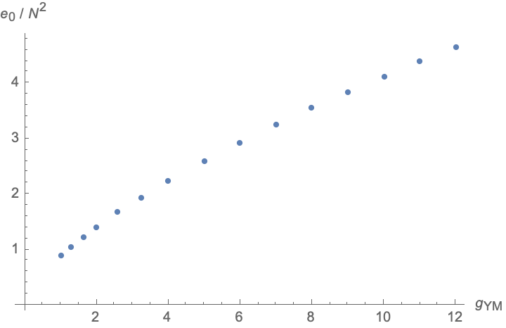
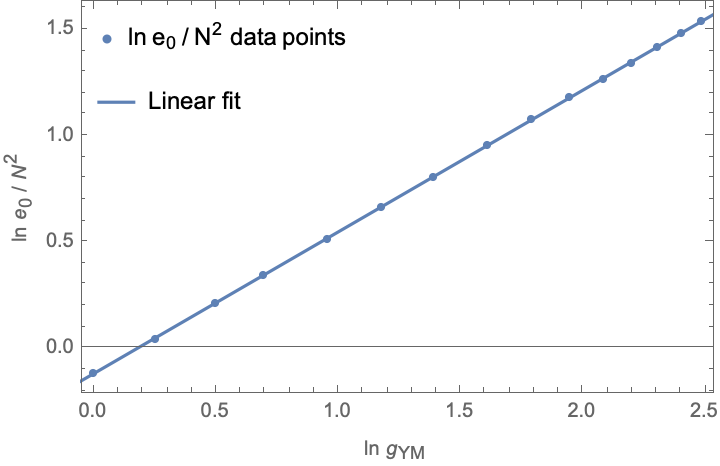
We fit the data to the curve
by performing a linear regression (least squares) fit to the logarithmic plot. We find:
This linear fit is shown in Figure 2.
| 1.0 | 1.28403 | 1.64872 | 2.0 | 2.6 | 3.25 | 4.0 | 5.0 | 6.0 | 7.0 | 8.0 | 9.0 | 10.0 | 11.0 | 12.0 | |
| 0.88904 | 1.05027 | 1.24075 | 1.41124 | 1.68099 | 1.95060 | 2.24021 | 2.59951 | 2.93549 | 3.25320 | 3.55622 | 3.84669 | 4.12662 | 4.39716 | 4.65995 | |
| 1.0000 | 1.0000 | 1.0000 | 1.0000 | 1.0000 | 1.0000 | 1.0000 | 1.0000 | 1.0000 | 1.0000 | 1.0000 | 1.0000 | 1.0000 | 1.0000 | 1.0000 | |
| 0.0000 | 0.0000 | 0.0000 | 0.0000 | 0.0001 | 0.0000 | 0.0000 | 0.0000 | 0.0000 | 0.0000 | -0.0001 | 0.0000 | -0.0001 | 0.0000 | 0.0000 | |
| 0.0000 | 0.0000 | 0.0003 | 0.0000 | 0.0000 | 0.0000 | 0.0000 | 0.0000 | 0.0000 | 0.0000 | 0.0000 | 0.0000 | 0.0000 | 0.0000 | 0.0000 | |
| 0.4651 | 0.3937 | 0.3333 | 0.2931 | 0.2460 | 0.2120 | 0.1846 | 0.1591 | 0.1409 | 0.1271 | 0.1163 | 0.1075 | 0.1002 | 0.0941 | 0.0887 | |
| 0.0000 | 0.0000 | 0.0000 | 0.0000 | 0.0000 | 0.0000 | 0.0000 | 0.0000 | 0.0000 | 0.0000 | 0.0000 | 0.0000 | 0.0000 | 0.0000 | 0.0000 | |
| 0.4651 | 0.3937 | 0.3333 | 0.2930 | 0.2460 | 0.2120 | 0.1846 | 0.1591 | 0.1409 | 0.1271 | 0.1163 | 0.1075 | 0.1002 | 0.0941 | 0.0887 | |
| 0.0000 | 0.0000 | 0.0001 | 0.0000 | 0.0001 | 0.0000 | 0.0000 | 0.0000 | 0.0000 | 0.0000 | -0.0001 | 0.0000 | 0.0000 | 0.0000 | 0.0000 | |
| 0.0000 | 0.0000 | 0.0001 | 0.0000 | 0.0000 | 0.0000 | 0.0000 | 0.0000 | 0.0000 | 0.0000 | 0.0000 | 0.0000 | 0.0000 | 0.0000 | 0.0000 | |
| 0.0000 | 0.0000 | 0.0000 | 0.0000 | 0.0000 | 0.0000 | 0.0000 | 0.0000 | 0.0000 | 0.0000 | 0.0000 | 0.0000 | 0.0000 | 0.0000 | 0.0000 | |
| -0.0001 | 0.0000 | 0.0003 | 0.0000 | 0.0000 | 0.0000 | 0.0000 | 0.0000 | 0.0000 | 0.0000 | 0.0000 | 0.0000 | 0.0000 | 0.0000 | 0.0000 | |
| 0.4364 | 0.3127 | 0.2241 | 0.1732 | 0.1221 | 0.0907 | 0.0687 | 0.0511 | 0.0400 | 0.0326 | 0.0273 | 0.0233 | 0.0203 | 0.0178 | 0.0159 | |
| 0.0000 | 0.0000 | 0.0000 | 0.0000 | 0.0000 | 0.0000 | 0.0000 | 0.0000 | 0.0000 | 0.0000 | 0.0000 | 0.0000 | 0.0000 | 0.0000 | 0.0000 | |
| 0.1949 | 0.1396 | 0.1001 | 0.0773 | 0.0545 | 0.0405 | 0.0307 | 0.0228 | 0.0179 | 0.0146 | 0.0122 | 0.0104 | 0.0090 | 0.0080 | 0.0071 | |
| 0.0467 | 0.0334 | 0.0240 | 0.0185 | 0.0131 | 0.0097 | 0.0074 | 0.0055 | 0.0043 | 0.0035 | 0.0029 | 0.0025 | 0.0022 | 0.0019 | 0.0017 | |
| 0.0000 | 0.0000 | 0.0000 | 0.0000 | 0.0000 | 0.0000 | 0.0000 | 0.0000 | 0.0000 | 0.0000 | 0.0000 | 0.0000 | 0.0000 | 0.0000 | 0.0000 | |
| 0.4364 | 0.3127 | 0.2241 | 0.1732 | 0.1221 | 0.0907 | 0.0687 | 0.0511 | 0.0400 | 0.0326 | 0.0273 | 0.0233 | 0.0202 | 0.0178 | 0.0159 | |
| ”angle” | 0.68489 | 0.68488 | 0.68482 | 0.68478 | 0.68477 | 0.68472 | 0.68474 | 0.68472 | 0.68472 | 0.68471 | 0.68518 | 0.68513 | 0.68516 | 0.68466 | 0.68516 |
| 1,00 | 1,28 | 1,65 | 2,00 | 2,60 | 3,25 | 4,00 | 5,00 | 6,00 | 7,00 | 8,00 | 9,00 | 10,00 | 11,00 | 12,00 | ||
| Energy | 0.88904 | 1.05027 | 1.24075 | 1.41124 | 1.68099 | 1.95060 | 2.24021 | 2.59951 | 2.93549 | 3.25320 | 3.55622 | 3.84669 | 4.12662 | 4.39716 | 4.65995 | |
| 0 | 1.0000 | 1.0000 | 1.0000 | 1.0000 | 1.0000 | 1.0000 | 1.0000 | 1.0000 | 1.0000 | 1.0000 | 1.0000 | 1.0000 | 1.0000 | 1.0000 | 1.0000 | |
| 1 | 0.0000 | 0.0000 | 0.0000 | 0.0000 | 0.0000 | -0.0000 | 0.0000 | 0.0000 | 0.0000 | -0.0001 | -0.0000 | -0.0000 | -0.0000 | -0.0000 | 0.0000 | |
| -1 | 0.0000 | 0.0000 | 0.0000 | 0.0000 | 0.0000 | -0.0000 | 0.0000 | 0.0000 | 0.0000 | -0.0001 | -0.0000 | -0.0000 | -0.0000 | -0.0000 | 0.0000 | |
| 2 | 0.0000 | 0.0000 | -0.0000 | 0.0000 | -0.0000 | -0.0000 | 0.0000 | -0.0000 | -0.0000 | 0.0000 | -0.0000 | 0.0000 | 0.0000 | -0.0000 | 0.0000 | |
| 0 | 0.9303 | 0.7874 | 0.6665 | 0.5861 | 0.4920 | 0.4240 | 0.3692 | 0.3182 | 0.2818 | 0.2542 | 0.2325 | 0.21500 | 0.2004 | 0.1881 | 0.1774 | |
| -2 | 0.0000 | 0.0000 | -0.0000 | 0.0000 | -0.0000 | -0.0000 | 0.0000 | -0.0000 | -0.0000 | 0.0000 | 0.0000 | 0.0000 | -0.0000 | 0.0000 | 0.0000 | |
| 3 | 0.0000 | 0.0000 | 0.0000 | 0.0000 | -0.0000 | 0.0000 | -0.0000 | -0.0000 | 0.0000 | -0.0000 | -0.0000 | -0.0000 | 0.0000 | 0.0000 | -0.0000 | |
| 1 | 0.0000 | 0.0000 | 0.0000 | 0.0000 | 0.0000 | -0.0000 | 0.0000 | 0.0000 | 0.0000 | 0.0000 | -0.0000 | -0.0000 | -0.0000 | -0.0000 | -0.0000 | |
| -1 | 0.0000 | 0.0000 | 0.0000 | 0.0000 | 0.0000 | -0.0000 | 0.0000 | 0.0000 | 0.0000 | 0.0000 | -0.0000 | -0.0000 | -0.0000 | -0.0000 | -0.0000 | |
| -3 | 0.0000 | 0.0000 | 0.0000 | 0.0000 | -0.0000 | 0.0000 | -0.0000 | -0.0000 | 0.0000 | -0.0000 | -0.0000 | -0.0000 | 0.0000 | 0.0000 | -0.0000 | |
| 4 | 0.0000 | 0.0000 | 0.0000 | -0.0000 | 0.0000 | -0.0000 | 0.0000 | -0.0000 | -0.0000 | -0.0000 | -0.0000 | 0.0000 | 0.0000 | 0.0000 | -0.0000 | |
| 2 | 0.0000 | 0.0000 | -0.0000 | 0.0000 | 0.0000 | 0.0000 | 0.0000 | 0.0000 | -0.0000 | -0.0000 | -0.0000 | -0.0000 | 0.0000 | 0.0000 | 0.0000 | |
| 0 | 0.9662 | 0.6923 | 0.4961 | 0.3835 | 0.2703 | 0.2008 | 0.1522 | 0.1130 | 0.0886 | 0.0722 | 0.0604 | 0.0515 | 0.0448 | 0.0395 | 0.0352 | |
| 0 | 1.5589 | 1.11698 | 0.8004 | 0.6187 | 0.4361 | 0.3239 | 0.2456 | 0.1824 | 0.1430 | 0.1164 | 0.0974 | 0.0832 | 0.0723 | 0.0637 | 0.0567 | |
| -2 | 0.0000 | 0.0000 | -0.0000 | 0.0000 | 0.0000 | 0.0000 | 0.0000 | 0.0000 | -0.0000 | -0.0000 | -0.0000 | -0.0000 | 0.0000 | 0.0000 | 0.0000 | |
| -4 | 0.0000 | 0.0000 | -0.0000 | 0.0000 | 0.0000 | 0.0000 | 0.0000 | 0.0000 | -0.0000 | -0.0000 | -0.0000 | -0.0000 | 0.0000 | 0.0000 | 0.0000 |
The accuracy with which the interpolation matches the exact scaling at this level of truncation is remarkable 151515The parameters and their uncertainties are obtained with the Mathematica functions LinearModelFit and NonlinearModelFit. Note that the fit uncertainties are remarkably consistent with the estimated numerical errors associated with this level of loop truncation.. We are then justified in setting and fit the data to the scaling function
| (9) |
with result
| (10) |
Figure 3 displays the fit of the large planar ground state energies to the scaling function (9) with parameter (10). Again, the level of accuracy (10) with which the numerically obtained planar ground state energies match the scaling behaviour (9) at this level of truncation is remarkable.
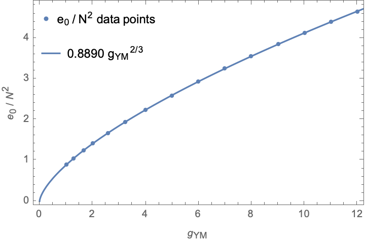
Taking into account possible truncation dependent errors, as estimated in Appendix A, we then list the final scaling dependence on ’t Hooft’s coupling for the planar ground state energy of the massless system as:
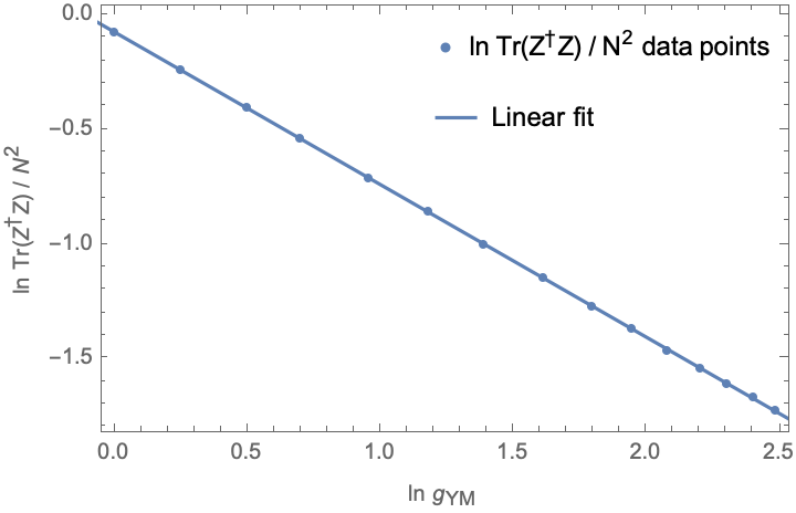
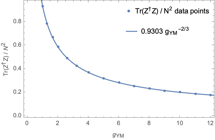
We follow the same analysis for loops with two matrices and consider the correlator . The logarithmic dependence is first approximated by a linear fit, and then matched to the scaling dimensions of the loop correlator:
The results are presented in table 5 and displayed in Figure 4.
| Parameters of (log) linear fit | fixed | Final scaling function | |
|---|---|---|---|
| -0.07219(7) | -0.66672(4) | 0.93027(3) | |
The scaling power for the large planar correlator is again predicted with a high level of accuracy, and their numerical values match with a high level of precision the scaling behaviour. The numerical errors associated with the loop truncation are estimated in Appendix A, and taken into account in the final scaling function presented in table 5.
For invariant loops with matrices, we consider the loops and , and carry out the same analysis, which is summarized in table 6 and figure 5.
| Log linear fit | Final | |||
|---|---|---|---|---|
| Scaling function | ||||
| 0.4441(1) | -1.33340(6) | 1.55895(8) | ||
| -0.0342(2) | -1.3334(1) | 0.96626(8) | ||
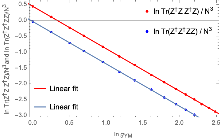
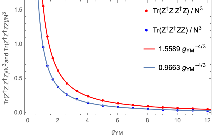
Remarks similar to those given for the previously discussed large planar quantities which concern the high level of accuracy of the numerical results, apply to the invariant loops with matrices considered in this case too.
Finally, we consider an ”angle” defined to be
For the integral with masses, and at large coupling, it has been shown that the two matrices commute [47]. For the quantum mechanical system in the massless limit, we observe, from the data listed in 3 that this ratio remains constant, and we obtain
Again, taking into account possible numerical errors associated with the loop truncation, we obtain
In [42], the large YM quantum mechanics of two matrices with mass was considered, and it was there pointed out that this ratio seemed to show convergence to a constant value at large coupling. We have been able to establish what its value is directly in the massless limit, for all coupling values, with a high degree of accuracy.
3.2 spectrum
We consider in this subsection the numerical results obtained for the spectrum of the theory. These are independent of and are determined from the quadratic hamiltonian as fluctuations about the large planar background, as described in Section 2.3.
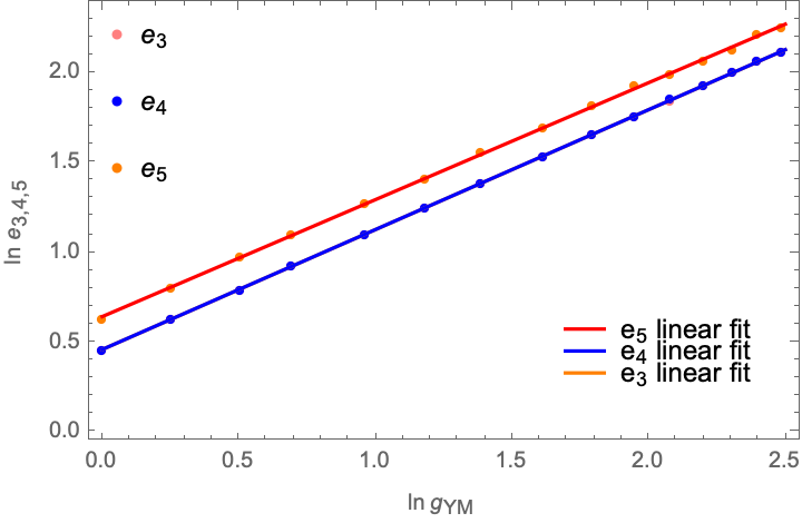
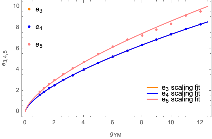
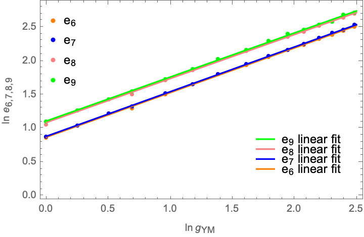
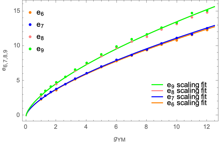
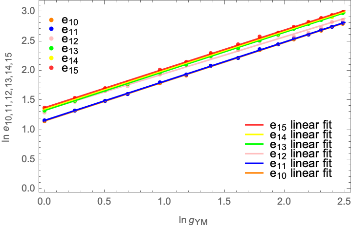
3.2.1 Masses and scaling behaviour
We observe that the mass of the third excited state and of all other higher excited states show the expected increase with coupling. The same is not the case for the two lowest lying states. We will first concentrate on the third and higher excited states, and discuss the two lowest lying states at the end of this subsection.
Numerically, one finds that the lowest lying states are determined quite accurately for small loop truncations, with the next higher lying states then becoming more accurate with larger number loops, and so on.
Table 7 displays the numerical results obtained for the masses of the rd to the th excited state 161616These would be particle states to particle states in the free system with a mass coupling. as a function of the coupling constant . Numerically, one finds that the lowest lying states are determined quite accurately for small loop truncations, with the next higher lying states then becoming more accurate with a larger number loops, and so on. Although the code generates data for all first excited states, we have chosen to list masses up to the th excited state as their masses are stable at this level of truncation. Truncation error estimates are presented in Appendix A.
We then carry out a similar analysis to that of previous subsection, by first performing a linear fit to the dependence of on the logarithm of , comparing it with the the scaling power prediction, and then optimize the match to the scaling dependence of the energies:
The are then adjusted to take into account truncation error estimates. The results are presented in table 8171717The somewhat unconventional notation say, instead of , is meant to help compare final parameter error estimates with those of the current ( loops) truncation level (in this case ) and highlight possible differences within possible multiplets..
| 1.0 | 1.28403 | 1.64872 | 2.0 | 2.6 | 3.25 | 4.0 | 5.0 | 6.0 | 7.0 | 8.0 | 9.0 | 10.0 | 11.0 | 12.0 | |
|---|---|---|---|---|---|---|---|---|---|---|---|---|---|---|---|
| 1.58783 | 1.87590 | 2.21627 | 2.52042 | 3.00208 | 3.48335 | 4.00097 | 4.64009 | 5.24314 | 5.80891 | 6.35076 | 6.87178 | 7.36991 | 7.84974 | 8.32061 | |
| 1.58826 | 1.87666 | 2.21658 | 2.52084 | 3.00301 | 3.48399 | 4.00108 | 4.64333 | 5.24456 | 5.80914 | 6.35230 | 6.87266 | 7.37212 | 7.85155 | 8.32270 | |
| 1.8817 | 2.2384 | 2.6469 | 2.9897 | 3.5754 | 4.1113 | 4.7403 | 5.4561 | 6.1860 | 6.8548 | 7.2816 | 7.8399 | 8.4051 | 9.1596 | 9.5306 | |
| 2.3624 | 2.8549 | 3.3788 | 3.6678 | 4.5283 | 5.2501 | 6.0686 | 6.9439 | 7.8667 | 8.6501 | 9.4171 | 10.217 | 10.864 | 11.630 | 12.340 | |
| 2.4227 | 2.8614 | 3.3845 | 3.8005 | 4.5699 | 5.2754 | 6.0982 | 7.0592 | 8.0208 | 8.7401 | 9.5187 | 10.368 | 11.175 | 11.731 | 12.574 | |
| 2.8920 | 3.5499 | 4.2006 | 4.5165 | 5.6054 | 6.4257 | 7.4950 | 8.5833 | 9.7959 | 10.620 | 11.343 | 12.400 | 13.159 | 14.118 | 14.850 | |
| 3.0224 | 3.5679 | 4.2135 | 4.7529 | 5.6196 | 6.5906 | 7.6095 | 8.7697 | 9.9158 | 10.999 | 11.722 | 12.656 | 13.328 | 14.740 | 15.106 | |
| 3.1770 | 3.7796 | 4.4787 | 4.9936 | 6.0322 | 6.9061 | 8.0139 | 9.2056 | 10.538 | 11.536 | 12.659 | 13.720 | 14.655 | 15.607 | 16.529 | |
| 3.2119 | 3.7908 | 4.4854 | 5.0488 | 6.0746 | 7.0056 | 8.0833 | 9.2782 | 10.605 | 11.620 | 12.732 | 13.763 | 14.762 | 15.718 | 16.576 | |
| 3.6644 | 4.3828 | 5.2722 | 5.7622 | 7.0210 | 8.1770 | 9.3819 | 10.537 | 12.173 | 13.366 | 13.179 | 14.243 | 15.329 | 17.050 | 17.522 | |
| 3.7820 | 4.5010 | 5.3748 | 5.9431 | 7.2252 | 8.2713 | 9.4737 | 10.789 | 12.494 | 13.589 | 15.134 | 16.433 | 17.470 | 18.407 | 19.565 | |
| 3.9256 | 4.5641 | 5.4285 | 6.0557 | 7.3141 | 8.4786 | 9.8013 | 11.268 | 12.813 | 13.813 | 15.230 | 16.737 | 17.774 | 18.540 | 19.990 | |
| 3.9768 | 4.6918 | 5.5272 | 6.1198 | 7.5254 | 8.6510 | 10.060 | 11.526 | 13.202 | 14.089 | 15.555 | 16.916 | 18.021 | 18.930 | 20.128 | |
| 3.9904 | 4.7478 | 5.6144 | 6.3157 | 7.5563 | 8.7746 | 10.124 | 11.600 | 13.250 | 14.597 | 15.666 | 16.972 | 18.166 | 19.639 | 20.415 | |
| 4.2782 | 5.1428 | 6.0890 | 6.7240 | 8.1507 | 9.1677 | 10.767 | 12.325 | 13.917 | 15.308 | 17.491 | 18.728 | 20.168 | 20.714 | 22.509 | |
| 4.7181 | 5.5377 | 6.6292 | 7.1827 | 8.8371 | 10.081 | 11.790 | 13.342 | 15.513 | 16.652 | 18.382 | 19.823 | 21.356 | 22.874 | 23.684 | |
| 4.7579 | 5.6074 | 6.6581 | 7.4679 | 8.9802 | 10.353 | 11.879 | 13.656 | 15.716 | 17.144 | 18.613 | 20.155 | 21.445 | 23.092 | 24.225 | |
| 4.7994 | 5.6289 | 6.6876 | 7.5628 | 9.1130 | 10.473 | 12.018 | 13.895 | 15.768 | 17.276 | 18.952 | 20.882 | 22.208 | 23.219 | 25.016 | |
| 4.8160 | 5.6543 | 6.7112 | 7.6996 | 9.1279 | 10.549 | 12.048 | 13.920 | 15.935 | 17.511 | 19.144 | 20.921 | 22.451 | 23.420 | 25.119 | |
| 5.0709 | 5.8664 | 7.0180 | 7.9112 | 9.4813 | 11.056 | 12.703 | 14.521 | 16.572 | 18.178 | 19.980 | 21.713 | 23.141 | 24.453 | 26.087 | |
| 5.1189 | 5.9758 | 7.1513 | 8.0451 | 9.6420 | 11.162 | 12.899 | 14.915 | 16.728 | 18.454 | 20.172 | 21.979 | 23.337 | 24.548 | 26.198 | |
| 5.5177 | 6.4132 | 7.7126 | 8.6924 | 10.400 | 11.973 | 13.669 | 15.655 | 18.175 | 19.692 | 21.818 | 23.843 | 25.621 | 26.910 | 28.568 | |
| 5.5663 | 6.5097 | 7.7646 | 8.8801 | 10.577 | 12.156 | 14.062 | 15.994 | 18.407 | 20.141 | 22.037 | 24.103 | 25.747 | 27.387 | 29.097 | |
| 5.6155 | 6.6611 | 7.8974 | 8.8917 | 10.701 | 12.409 | 14.195 | 16.348 | 18.606 | 20.372 | 22.472 | 24.597 | 26.309 | 27.733 | 29.533 | |
| 5.6549 | 6.7057 | 7.9368 | 8.9654 | 10.722 | 12.487 | 14.344 | 16.464 | 18.706 | 20.675 | 22.619 | 24.643 | 26.417 | 27.766 | 29.735 | |
| 5.9641 | 6.8887 | 8.2739 | 9.4674 | 11.256 | 12.937 | 14.844 | 16.996 | 19.266 | 21.269 | 23.800 | 25.686 | 27.749 | 29.054 | 31.282 | |
| 6.0821 | 7.0254 | 8.3083 | 9.4841 | 11.329 | 13.063 | 15.009 | 17.416 | 19.623 | 21.800 | 24.063 | 26.090 | 27.884 | 29.207 | 31.400 | |
| 6.1661 | 7.1322 | 8.5372 | 9.6920 | 11.623 | 13.387 | 15.364 | 17.831 | 20.078 | 22.169 | 24.848 | 26.217 | 28.152 | 29.996 | 31.865 | |
| 6.3174 | 7.5318 | 8.8912 | 9.9197 | 11.876 | 13.525 | 15.821 | 18.185 | 20.581 | 22.576 | 25.696 | 28.703 | 30.412 | 30.253 | 34.036 | |
| 6.4214 | 7.7110 | 9.0560 | 10.269 | 12.467 | 14.282 | 16.409 | 18.871 | 21.506 | 23.665 | 26.221 | 28.788 | 30.709 | 32.035 | 34.632 | |
| 6.4975 | 7.7573 | 9.0860 | 10.373 | 12.514 | 14.618 | 16.617 | 19.174 | 21.600 | 23.724 | 26.621 | 29.246 | 31.143 | 32.371 | 35.148 | |
| 6.7837 | 8.0036 | 9.4812 | 10.756 | 12.904 | 14.845 | 16.954 | 19.663 | 22.339 | 24.689 | 26.737 | 29.415 | 31.332 | 33.115 | 35.432 | |
| 6.7997 | 8.0186 | 9.4927 | 10.793 | 12.944 | 14.877 | 17.047 | 19.847 | 22.377 | 24.816 | 27.003 | 29.730 | 31.483 | 33.359 | 35.767 | |
| 6.9259 | 8.0801 | 9.6280 | 10.935 | 13.037 | 15.090 | 17.302 | 19.985 | 22.726 | 24.963 | 27.355 | 29.820 | 32.145 | 33.537 | 36.135 | |
| 7.0077 | 8.2133 | 9.7493 | 11.030 | 13.209 | 15.377 | 17.472 | 20.177 | 23.011 | 25.253 | 27.864 | 29.948 | 32.250 | 34.672 | 36.447 |
| Log linear fit | fixed | Final | ||
|---|---|---|---|---|
| n | Scaling function | |||
| 0.4624(1) | 0.66657(7) | 1.58767(9) | ||
| 0.4627(1) | 0.66656(6) | 1.58806(8) | ||
| 0.645(6) | 0.650(3) | 1.862(8) | ||
| 0.873(6) | 0.660(4) | 2.373(8) | ||
| 0.885(3) | 0.661(2) | 2.406(5) | ||
| 1.09(1) | 0.651(6) | 2.91(2) | ||
| 1.112(7) | 0.652(4) | 2.98(1) | ||
| 1.159(3) | 0.663(2) | 3.170(5) | ||
| 1.167(2) | 0.662(1) | 3.191(5) | ||
| 1.34(2) | 0.62(1) | 3.57(5) | ||
| 1.336(6) | 0.660(3) | 3.77(1) | ||
| 1.361(5) | 0.657(3) | 3.85(1) | ||
| 1.382(7) | 0.655(4) | 3.92(2) | ||
| 1.393(4) | 0.657(3) | 3.97(1) | ||
| 1.457(9) | 0.663(5) | 4.27(2) | ||
| 1.547(7) | 0.656(4) | 4.62(2) | ||
| 1.563(3) | 0.656(2) | 4.70(1) | ||
| 1.567(4) | 0.663(2) | 4.770(9) | ||
| 1.572(3) | 0.665(2) | 4.802(8) | ||
| 1.615(4) | 0.663(2) | 5.001(9) | ||
| 1.633(4) | 0.659(2) | 5.07(1) | ||
| 1.701(5) | 0.664(3) | 5.46(1) | ||
| 1.716(3) | 0.665(2) | 5.547(9) | ||
| 1.728(3) | 0.666(2) | 5.631(8) | ||
| 1.735(2) | 0.666(1) | 5.666(6) | ||
| 1.776(6) | 0.666(3) | 5.90(1) | ||
| 1.790(4) | 0.665(2) | 5.98(1) | ||
| 1.812(4) | 0.664(3 | 6.10(1) | ||
| 1.83(1) | 0.673(8) | 6.32(4) | ||
| 1.866(5) | 0.673(3) | 6.52(2) | ||
| 1.874(6) | 0.675(4) | 6.59(2) | ||
| 1.916(3) | 0.663(2) | 6.76(1) | ||
| 1.917(3) | 0.666(2) | 6.793(9) | ||
| 1.930(3) | 0.664(2) | 6.87(1) | ||
| 1.943(3) | 0.665(2) | 6.960(9) | ||
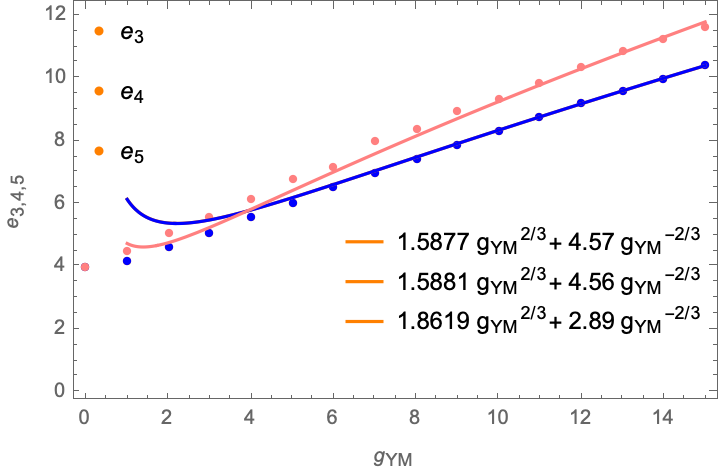
Again we observe an excellent agreement with the expected scaling power of the coupling constant for the masses of the excited states, typically with uncertainties below the level181818The mass is an intriguing discrepancy that may require further later re-examination. However, the quality of its fit to the scaling power law is in line with other excited states.. The two degenerate massive lowest lying states and , of particular physical relevance, are specially accurate.
In figures 6 , 7 and 8, we display the logarithmic linear fits and the fits to the scaling power law of the numerical spectrum data for . This illustrates the patterns of degeneracy, which will be further discussed in the next subsection.
3.2.2 charges
The assignment of charges to the different multiplets is more cleanly carried out in a complex matrices loop basis:
| (11) | |||||
This defines a (complex valued) linear transformation between the complex matrices loop components of a mass eigenvector and its hermitian matrices loop components. It is block diagonal, and as such one can carry out the analysis for each sector of fixed particle number.
We find that the pattern of degeneracies is best evidenced by considering spectra corresponding to truncation subsectors within the planar background ([44]). In this subsection, we base our discussion on a truncation for .
On general grounds, states with non-zero charges should come in doublets . It should be remembered, though, that the present numerical approach is based on hermitian matrices parametrized by real master variables. So typically, the eigenvector components are real. To obtain states of definite charge, the two degenerate eigenvectors have to first be expressed in a complex matrices loop component basis using (3.2.2) and then the linear combinations identified that yield two states of definite opposite charges.
To illustrate the procedure, we display in table 9 the components of the eigenvectors and . The states and are degenerate. As it can be observed from (3.2.2), they essentially ”group” the real and imaginary parts of the states: , with the imaginary part. For the singlet, one has with no imaginary part.
| Doublet | Singlet | ||
|---|---|---|---|
| 0.0643 | -0.0401 | 0.0055 | |
| 0.0830 | 0.1247 | 0.0000 | |
| -0.0643 | 0.0403 | 0.0055 | |
After re-writing the doublet states in a complex matrices loop component basis, one performs the linear combination required to obtain the (chiral) states of definite charge.
The choice of the linear combination coefficients is determined within the particle sector, but they act on the full eigenvector. The first components of the states are displayed in table 10. By construction, and are set to . The table confirms the vanishing of all other components (numerically less than ), except for and . These -particle components also carry charges , respectively, and their enhancement to about results from the fact that the Hamiltonian, unlike the dilatation operator or upon radial quantization, is not number conserving.
| [ZZ] | 1.000 +i0.000 | 0.000 +i0.000 |
|---|---|---|
| -0.001 +i0.001 | -0.001- i0.001 | |
| 0.000 +i0.000 | 1.000 +i0.000 | |
| 0.000 +i0.000 | 0.001 +i0.002 | |
| 0.000 +i0.000 | -0.005 -i0.006 | |
| -0.005 +i0.006 | 0.000 -i0.000 | |
| 0.001 -i0.002 | 0.000 -i0.000 | |
| 0.001 -i0.000 | 0.003 +i0.002 | |
| 0.091 +i0.002 | 0.005 -i0.008 | |
| 0.007 +i0.002 | 0.007 -i0.002 | |
| 0.002 +i0.002 | 0.002 -i0.002 | |
| 0.005 +i0.008 | 0.091 -i0.002 | |
| 0.003 -i0.002 | 0.001 +i0.000 | |
| Charge |
We consider now the next states . They appear as two doubly degenerate states. Their components are displayed in table 11. Again, they ”encode” real and imaginary parts of definite charge states, as can be seen by inspection of (3.2.2) : and similarly for , whereas , and similarly for .
| Doublet | Doublet | |||
|---|---|---|---|---|
| 0.1403 | -0.1403 | -0.0238 | 0.0174 | |
| 0.4269 | 0.4104 | -0.0184 | -0.0239 | |
| -0.4112 | 0.4225 | -0.0243 | 0.0158 | |
| -0.1398 | -0.1340 | -0.0159 | -0.0228 | |
Expressing the doublet states in complex matrices loop components, and performing linear combinations within each doublet to obtain states of definite charge, one obtains table 12. Other than , ,, , all set to one, the other components vanish to within for the doublet and within for the doublet.
| Doublet | Doublet | |||
| [ZZ] | 0.003+i0.000 | -0.005 +i0.003 | 0.002 -i0.005 | -0.006 -i0.015 |
| -0.013 +i0.007 | -0.013 -i0.007 | 0.007 +i0.011 | 0.007 -i0.011 | |
| -0.005 -i0.003 | 0.003 -i0.000 | -0.006 +i0.015 | 0.002 +i0.005 | |
| 1.000 +i0.000 | 0.000 +i0.000 | 0.012 -i0.013 | -0.008 +i0.001 | |
| 0.011 +i0.006 | -0.003 -i0.005 | 1.000 +i0.000 | 0.000 +i0.000 | |
| -0.003 +i0.005 | 0.011 -i0.006 | 0.000 +i0.000 | 1.000 +i0.000 | |
| 0.000 +i0.000 | 1.000 +i0.000 | -0.008 -i0.001 | 0.012 +i0.013 | |
| 0.004 -i0.008 | -0.003 -i0.001 | -0.017 +i0.060 | 0.003 +i0.033 | |
| -0.011 +i0.005 | 0.026 -i0.026 | -0.003 +i0.015 | -0.043 +i0.052 | |
| 0.026 -i0.060 | 0.026 +i0.060 | -0.005 -i0.026 | -0.005 +i0.026 | |
| 0.015 -i0.009 | 0.015 +i0.009 | 0.006 -i0.010 | 0.006 +i0.010 | |
| 0.026 +i0.026 | -0.011 -i0.005 | -0.043 -i0.052 | -0.003 -i0.015 | |
| -0.003 +i0.001 | 0.004 +i0.008 | 0.003 -0.i033 | -0.017 -i0.060 | |
| Charge | ||||
The procedure should by now be clear, and we present the assignment of non-zero charges to the states - in table 13. Again, components vanish to within less than , except for those set to , and the -particle components and , also with charges. Interestingly, as that need not be the case, the states are also degenerate. A summary of the charge assignments of the states is presented in table 14.
| Doublet | Doublet | |||
| [ZZ] | 0.008+i0.004 | 0.005-i0.002 | -0.472+i0.007 | -0.016+i0.006 |
| -0.005+i0.000 | -0.005-i0.000 | 0.043+i0.020 | 0.0430-i0.020 | |
| 0.005+i0.002 | 0.008-i0.004 | -0.016-i0.006 | -0.472-i0.007 | |
| -0.004+i0.004 | -0.000-i0.000 | 0.004-i0.018 | 0.009-i0.002 | |
| -0.046+i0.079 | 0.043-i0.004 | -0.000+i0.001 | -0.009+i0.012 | |
| 0.043+i0.004 | -0.046-i0.079 | -0.009-i0.012 | -0.000-i0.001 | |
| -0.000+i0.000 | -0.004-i0.004 | 0.009+i0.002 | 0.004+i0.018 | |
| 1.000+i0.000 | -0.000+i0.000 | 0.021-i0.013 | -0.033+i0.009 | |
| -0.025-i0.002 | -0.021+i0.027 | 1.000+i0.000 | -0.000+i0.000 | |
| 0.008+i0.005 | 0.008-i0.005 | -0.041-i0.030 | -0.041+i0.030 | |
| 0.002+i0.001 | 0.002-i0.001 | -0.023-i0.009 | -0.023+i0.009 | |
| -0.021-i0.027 | -0.025+i0.002 | 0.000+i0.000 | 1.000+i0.000 | |
| -0.000+i0.000 | 1.000-i0.000 | -0.033-i0.009 | 0.021+i0.013 | |
| Charge | ||||
| Degeneracy | Charge | |
|---|---|---|
| doublet | ||
| singlet | ||
| doublet | ||
| doublet | ||
| doublet | ||
| doublet | ||
| doublet |
The approach can be extended for higher states, but it is clear that a more efficient and systematic way to do so would be to start directly with two complex matrices. This is under current investigation, but beyond the scope of this communication.
3.2.3 Massless excitations
We now turn our attention to the lowest excited sates and . Numerically, their masses do not increase with the coupling, and remain very small compared with the other massive excited states. These are the traced constituent single particle states and , and we associate them with the non interacting (free) subgroup of (8). Numerically, one should be reminded that the eigenvalues of the mass matrix (7) include unphysical zero eigenvalues, so these modes will mix with physical zero modes if present in the system. In order to confirm numerically that, indeed, our interpretation that and are decoupled zero mass states, we ”switch on” masses in the Hamiltonian and seek evidence that indeed and remain decoupled states with masses equal to their ”bare” masses. This will also allow us to compare our results with the few planar results available in the literature. This is carried out in the next section.
4 Yang-Mills coupled Hamiltonian with mass
In this section, we consider the matrix quantum mechanical Hamiltonian
| (12) |
The same loop truncation with loops () and a matrix is used. We fix and take . Numerical results for the planar large energy, the planar even loop correlator values, the planar complex matrices loop correlator values,191919The loop correlators with an odd number of any of the hermitian matrices are numerically to decimal places with very few exceptions, where their values do not exceed , and similarly for complex matrices loop correlators with non-zero charges. As such, they are not displayed. and the first mass spectra are displayed in table 15.
| 0 | 1 | 2 | 3 | 4 | 5 | 6 | 7 | 8 | 9 | 10 | 11 | 12 | 13 | 14 | 15 | |
|---|---|---|---|---|---|---|---|---|---|---|---|---|---|---|---|---|
| 2.00000 | 2.10908 | 2.34396 | 2.61780 | 2.90090 | 3.18318 | 3.46097 | 3.73293 | 3.99883 | 4.25863 | 4.51261 | 4.76107 | 5.00439 | 5.24285 | 5.47664 | 5.70642 | |
| 1.0000 | 1.0000 | 1.0000 | 1.0000 | 1.0000 | 1.0000 | 1.0000 | 1.0000 | 1.0000 | 1.0000 | 1.0000 | 1.0000 | 1.0000 | 1.0000 | 1.0000 | 1.0000 | |
| 0.2500 | 0.2273 | 0.1946 | 0.1691 | 0.1499 | 0.1350 | 0.1232 | 0.1137 | 0.1057 | 0.0989 | 0.0931 | 0.0881 | 0.0837 | 0.0798 | 0.0763 | 0.0731 | |
| 0.2500 | 0.2273 | 0.1946 | 0.1691 | 0.1499 | 0.1350 | 0.1232 | 0.1136 | 0.1057 | 0.0989 | 0.0931 | 0.0881 | 0.0837 | 0.0798 | 0.0763 | 0.0731 | |
| 0.5000 | 0.4546 | 0.3892 | 0.3382 | 0.2998 | 0.2700 | 0.2464 | 0.2273 | 0.2114 | 0.1978 | 0.1862 | 0.1762 | 0.1674 | 0.1596 | 0.1526 | 0.1462 | |
| 0.1250 | 0.1034 | 0.0759 | 0.0574 | 0.0451 | 0.0367 | 0.0305 | 0.0260 | 0.0225 | 0.0197 | 0.0175 | 0.0156 | 0.0141 | 0.0128 | 0.0117 | 0.0108 | |
| 0.0625 | 0.0506 | 0.0362 | 0.0269 | 0.0210 | 0.0169 | 0.0140 | 0.0119 | 0.0102 | 0.0089 | 0.0079 | 0.0071 | 0.0064 | 0.0058 | 0.0053 | 0.0049 | |
| 0.0000 | 0.0021 | 0.0035 | 0.0035 | 0.0032 | 0.0029 | 0.0025 | 0.0023 | 0.0020 | 0.0018 | 0.0016 | 0.0015 | 0.0014 | 0.0012 | 0.0012 | 0.0011 | |
| 0.1250 | 0.1034 | 0.0759 | 0.0574 | 0.0451 | 0.0367 | 0.0306 | 0.0260 | 0.0225 | 0.0197 | 0.0175 | 0.0156 | 0.0141 | 0.0128 | 0.0117 | 0.0108 | |
| 0.2750 | 0.4050 | 0.2896 | 0.2154 | 0.1678 | 0.1352 | 0.1121 | 0.0950 | 0.0818 | 0.0714 | 0.0634 | 0.0566 | 0.0510 | 0.0464 | 0.0422 | 0.0390 | |
| 0.2500 | 0.2110 | 0.1588 | 0.1218 | 0.0966 | 0.0792 | 0.0661 | 0.0566 | 0.0490 | 0.0430 | 0.0382 | 0.0342 | 0.031 | 0.0280 | 0.0258 | 0.0238 | |
| 2.0000 | 2.0000 | 1.9995 | 1.9980 | 1.9954 | 1.9919 | 1.9887 | 1.9805 | 1.9798 | 1.9722 | 1.9674 | 1.9596 | 1.9536 | 1.9471 | 1.9279 | 1.9334 | |
| 2.0000 | 2.0000 | 1.9995 | 1.9981 | 1.9957 | 1.9925 | 1.9890 | 1.9819 | 1.9805 | 1.9728 | 1.9701 | 1.9606 | 1.9558 | 1.9483 | 1.9315 | 1.9384 | |
| 4.0000 | 4.2078 | 4.6242 | 5.0937 | 5.5751 | 6.0549 | 6.5295 | 6.9938 | 7.4520 | 7.8999 | 8.3399 | 8.7703 | 9.1924 | 9.6087 | 10.011 | 10.418 | |
| 4.0000 | 4.2080 | 4.6242 | 5.0937 | 5.5753 | 6.0556 | 6.5298 | 6.9946 | 7.4529 | 7.9006 | 8.3405 | 8.7714 | 9.1933 | 9.6094 | 10.013 | 10.419 | |
| 4.0000 | 4.5327 | 5.0772 | 5.5688 | 6.1573 | 6.7943 | 7.1861 | 8.0037 | 8.3936 | 8.9599 | 9.3389 | 9.8451 | 10.363 | 10.900 | 11.237 | 11.649 | |
| 5.5051 | 6.0541 | 6.9025 | 7.5558 | 8.3571 | 9.0595 | 9.5955 | 10.231 | 11.104 | 11.752 | 12.151 | 13.057 | 13.534 | 14.293 | 14.483 | 15.378 | |
| 5.9371 | 6.2794 | 6.9162 | 7.6186 | 8.3691 | 9.1177 | 9.8334 | 10.444 | 11.232 | 11.829 | 12.646 | 13.131 | 13.799 | 14.457 | 14.694 | 15.627 | |
| 5.9609 | 6.4296 | 7.1186 | 8.2597 | 9.6060 | 10.762 | 11.366 | 12.184 | 13.181 | 13.928 | 14.740 | 15.624 | 15.891 | 17.179 | 17.700 | 18.508 | |
| 5.9697 | 6.6118 | 7.6290 | 8.5949 | 9.8060 | 10.813 | 11.689 | 12.631 | 13.481 | 14.259 | 14.929 | 15.947 | 16.264 | 17.518 | 18.175 | 18.801 | |
| 7.8321 | 8.3047 | 7.7023 | 8.7651 | 9.8374 | 11.085 | 11.888 | 13.652 | 14.408 | 15.339 | 15.973 | 17.212 | 18.158 | 19.068 | 19.312 | 20.362 | |
| 7.8697 | 8.3887 | 9.1365 | 10.070 | 11.048 | 12.009 | 12.887 | 13.755 | 14.822 | 15.683 | 16.549 | 17.424 | 18.188 | 19.166 | 19.669 | 20.739 | |
| 7.8841 | 8.5108 | 9.1522 | 10.076 | 11.100 | 12.021 | 12.955 | 14.199 | 14.831 | 15.822 | 16.703 | 17.456 | 18.381 | 19.388 | 19.836 | 20.828 | |
| 7.9591 | 8.6885 | 9.8906 | 11.191 | 12.628 | 13.785 | 14.886 | 15.669 | 17.344 | 18.062 | 18.980 | 20.684 | 21.265 | 22.673 | 22.521 | 24.244 | |
| 7.9652 | 8.7147 | 9.9857 | 11.353 | 12.656 | 13.907 | 15.093 | 16.102 | 17.492 | 18.516 | 19.618 | 20.859 | 21.667 | 22.943 | 22.705 | 24.927 | |
| 7.9911 | 9.5729 | 10.056 | 11.655 | 13.323 | 14.743 | 15.942 | 16.575 | 18.284 | 19.388 | 20.456 | 21.426 | 21.988 | 23.350 | 23.117 | 25.383 |
4.1 Planar limit
Given that the leading large behaviour of the large energy, that of the massless limit, has been established in the previous section, we carry out a logarithmic fit of to for large to obtain the next, mass dependent, power dependence on . The logarithmic fit is shown in Figure 9 for . The least squares fit result for the exponent is , in other words to a high degree of accuracy. Setting , we obtain at this truncation level:
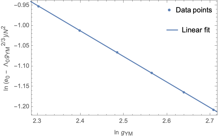
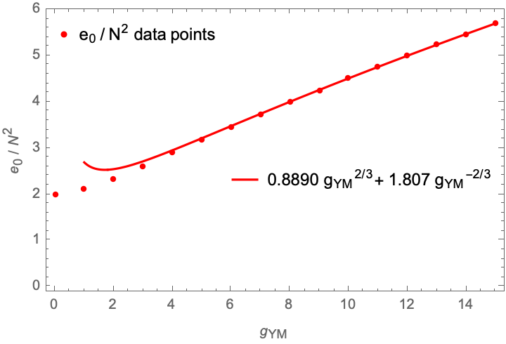
Since , one has
For , and large correlators, we limit ourselves in displaying the large scaling asymptotes. These are shown in Figure10
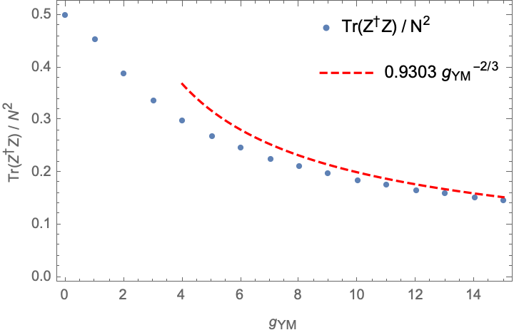
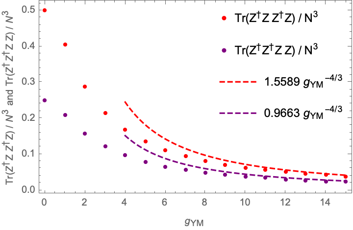
Table 16 compares our large planar results to those available in the literature.
For the large ground state energy, the improved accuracy of our approach is apparent. We also expect the leading dependence for to be the most accurate, as we are able to obtain it directly in the massless limit, whereas, as is evident from Figure 10, it may be difficult to extrapolate the leading dependence on from the strong coupling regime of an Hamiltonian with mass, as is the case in [42], [23].
4.2 spectrum
Inspection of table 15 shows that the energies and remain constant and very close to the ”bare” mass value 202020The slight decrease with is attributed to the fact that, numerically, the unphysical ”zero modes” develop small finite values. This is in opposition to the case of a quartic potential [44], and seemingly characteristic of a Yang-Mills potential in the context of our approach. In the massless limit then, these states remain massless, confirming the interpretation provided in the previous section.
This may be surprising from a diagrammatic point of view. Indeed, as an example, to order , one has the usual planar and non-planar contribution to the connected -point function , as shown in Figure 11.

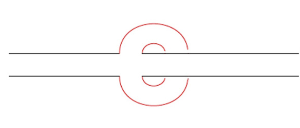
However, when the external legs are contracted, we see that the two diagrams of the previous figure cancel out, as shown in Figure 12


To the same order, one can also show diagramatically, for instance, the decoupling of -particle to -particle states212121Namely, the connected contribution to .
These are, however, simple perturbative results, but numerically it is established that, non-perturbatively, the states do not receive (finite) corrections to the ”bare” mass and decouple from higher (bound) states.
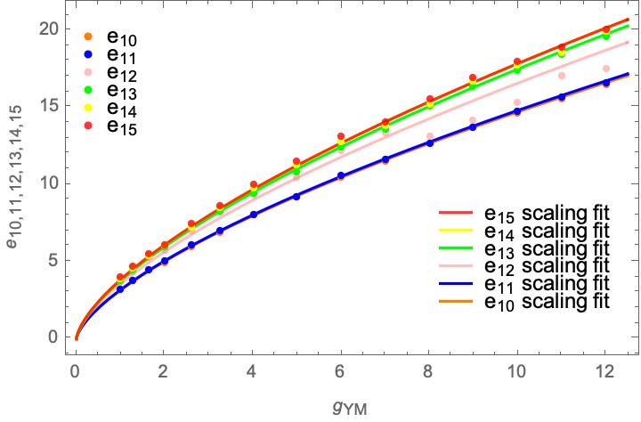
Finally, for the states with energies , we proceed as for to obtain the following mass corrected scaling functions:
or,
The above mass corrected scaling functions are displayed together with the numerically obtained energies in Figure 13. The agreement for the two lowest lying degenerate bound states at large is excellent.
There are no spectrum results available in the literature for comparison, as far as we know.
The assignment of charges is carried out in the same way as in the massless case, for and , and for a mass spectrum subsector on the full planar background. They are summarised in table 17 222222 The mass displays an irregular behaviour across the range of coupling constants, as was the case in the massless system. .
| n | Charge | |
|---|---|---|
| 8.34(1) | ||
| 8.34(1) | ||
| 9.3(4) | ||
| 12.2(2) | ||
| 12.6(5) | ||
| 15(1) | ||
| 15(1) | ||
| 16.0(8) | ||
| 16.5(2) | ||
| 16.7(1) | ||
| 19.0(2) | ||
| 19.6(1) | ||
| 20.5(9) |
5 Discussion and outlook
We studied the large N dynamics of two massless Yang-Mills coupled matrix quantum mechanics, by minimization of a loop truncated Jevicki-Sakita effective collective field Hamiltonian. The loop space constraints are handled by the use of master variables.
The method was successfully applied directly in the massless limit for a range of values of the Yang-Mills coupling constant, and the scaling behaviour of different physical quantities derived from their dimensions were obtained with a high level of precision. Planar correlators of non-zero charge were shown to vanish to a high degree of accuracy, and the expected charged spectrum degeneracies confirmed for a high number of states. This attests to the validity of the method, to the consistency of the truncation scheme and to the use of master variables.
We considered both planar properties of the theory, such as the large ground state energy and multi-matrix correlator expectation values, and also the spectrum of the theory.
For the spectrum, we established that the traced fundamental constituents remain massless and decoupled from other states, and that bound states develop well defined mass gaps, with the mass of the two degenerate lowest lying bound states being determined with a particularly high degree of accuracy. These results clarify whether the system has or does not have a mass gap, and establish the nature of its patterns.
As, potentially, the presence of massless states in the spectrum may present challenges in their identification, given the nature of the numerical scheme used, we also considered the case where the fundamental constituents have a finite ”bare mass”, and confirmed that their traced masses do not receive radiative corrections, and that they decouple from the remaining bound states in the spectrum. This also allowed us to compare some planar results with the small number of results available in the literature. As we are able to obtain the asymptotic large behaviour of different physical quantities directly in the massless limit, we expect our results to be more accurate for planar quantities, and new, for the spectrum with finite ”bare masses” as well.
Generalization to matrices, currently under investigation, is of clear physical interest, as is the possibility of adding large quenching to the master field construction. On the ”string/gravity” side, despite the absence of fermionic degrees of freedom and of a chiral limit, it is an interesting question to investigate if a BMN-type spectrum is present [52],[53],[54],[55],[56],[57] and other dual gravity properties. In this regard, the application of the method described in this article directly to complex matrices and chiral states is of interest, and currently under investigation. The addition of fermionic degrees of freedom and, more broadly, the generalization to supersymmetric systems is, of course, of great interest.
6 Appendix A - Effects of truncation parameters
In any numerical scheme involving a truncated system, it is important to try and estimate errors associated with the truncation itself, and with the different parameters of the algorithm. The accuracy of the numerical results presented in this article depend on three parameters: the truncation level (and corresponding ), (for a given ) and the convergence criterium of the optimization. We first discuss the loop truncation.
6.1 Loop truncation
The results presented in the main body of this article were obtained with , corresponding to a loop truncation involving the single trace operators with length less or equal to , and master variables (). is a matrix. For a few values of , we ran the optimization code for , corresponding to a loop truncation involving the single trace operators with length less or equal to , and master variables (). In this case, is a matrix. A number of planar quantities are displayed in tables 18 and 19 for , for both the massless case (18) and for mass (19).
The first observation is how accurate () the ground state energy is with respect to truncation dependence. For loops up to quartic loops, in general the accuracy is less than , except for a single loop where one can expect a truncation effect of . This is incorporated in the body of the article, where we have followed a very conservative approach and in general used the least accurate estimate.
| % diff. | % diff. | % diff. | |||||||
| 2.9355 | 2.9343 | 0.04% | 3.5562 | 3.5547 | 0.04% | 4.1266 | 4.1249 | 0.04% | |
| 1.0000 | 1.0000 | fixed | 1.0000 | 1.0000 | fixed | 1.0000 | 1.0000 | fixed | |
| 0.1409 | 0.1411 | -0.15 % | 0.1163 | 0.1164 | -0.17 % | 0.1002 | 0.1004 | -0.16% | |
| 0.1409 | 0.1411 | -0.16 % | 0.1163 | 0.1164 | -0.16 % | 0.1002 | 0.1004 | -0.16% | |
| 0.0400 | 0.0401 | -0.26% | 0.0273 | 0.0273 | -0.28 % | 0.0203 | 0.0203 | -0.26% | |
| 0.0179 | 0.0179 | -0.18% | 0.0122 | 0.0122 | -0.19% | 0.0090 | 0.0091 | -0.20% | |
| 0.0043 | 0.0043 | -0.90% | 0.0029 | 0.0029 | -0.92% | 0.0022 | 0.0022 | -0.98% | |
| 0.0400 | 0.0401 | -0.27% | 0.0273 | 0.0273 | -0.27% | 0.0202 | 0.0203 | -0.27% | |
| % diff. | % diff. | % diff. | |||||||
| 3.4610 | 3.4604 | 0.02% | 3.9988 | 3.9979 | 0.02% | 4.5126 | 4.5114 | 0.03% | |
| 1.0000 | 1.0000 | fixed | 1.0000 | 1.0000 | fixed | 1.0000 | 1.0000 | fixed | |
| 0.1232 | 0.1233 | -0.07% | 0.1057 | 0.1058 | -0.10% | 0.0931 | 0.0932 | -0.11% | |
| 0.1232 | 0.1233 | -0.07% | 0.1057 | 0.1058 | -0.10% | 0.0931 | 0.0932 | -0.12% | |
| 0.0305 | 0.0306 | -0.11% | 0.0225 | 0.0225 | -0.16% | 0.0175 | 0.0175 | -0.18% | |
| 0.0140 | 0.0140 | -0.06% | 0.0102 | 0.0102 | -0.10% | 0.0079 | 0.0079 | -0.12% | |
| 0.0025 | 0.0026 | -0.57% | 0.0020 | 0.0020 | -0.74% | 0.0016 | 0.0016 | -0.81% | |
| 0.0306 | 0.0306 | -0.11% | 0.0225 | 0.0225 | -0.16% | 0.0175 | 0.0175 | -0.19% | |
Tables 20 and 21 present similar results for the bound states to . We observe the accuracy of the two degenerate lowest lying bound states () and their insensitivity to truncation to within (). For higher states, the effects of the truncation vary from state to state, but except for in the massless case, they are found to be at most , with many states much less. The case of in the massless case displays larger truncation effects. Although requiring further understanding, these are the values used in the main body of the article, in line with our conservative approach to error estimation.
| % diff. | % diff. | % diff. | |||||||
| 5.2431 | 5.2368 | 0.12% | 6.3508 | 6.3436 | 0.11% | 7.3699 | 7.3605 | 0.13% | |
| 5.2446 | 5.2384 | 0.12% | 6.3524 | 6.3449 | 0.12% | 7.3721 | 7.3621 | 0.14% | |
| 6.1860 | 5.9766 | 3.39% | 7.2823 | 7.0897 | 2.64% | 8.4041 | 8.2057 | 2.36% | |
| 7.8667 | 7.6625 | 2.60% | 9.4180 | 9.2940 | 1.32% | 10.863 | 10.803 | 0.55% | |
| 8.0208 | 7.8264 | 2.42% | 9.5160 | 9.4329 | 0.87% | 11.175 | 10.861 | 2.81% | |
| 9.7959 | 9.0238 | 7.88% | 11.338 | 11.035 | 2.66% | 13.163 | 12.603 | 4.25% | |
| 9.9158 | 9.2379 | 6.84% | 11.717 | 11.099 | 5.27% | 13.324 | 12.969 | 2.66% | |
| 10.538 | 10.437 | 0.96% | 12.661 | 12.590 | 0.56% | 14.655 | 14.558 | 0.66% | |
| 10.605 | 10.466 | 1.31% | 12.732 | 12.700 | 0.25% | 14.763 | 14.617 | 0.99% | |
| 12.174 | 10.946 | 10.1% | 13.181 | 12.785 | 3.01% | 15.327 | 14.786 | 3.53% | |
| 12.494 | 12.303 | 1.53% | 15.133 | 14.682 | 2.98% | 17.465 | 17.019 | 2.56% | |
| 12.813 | 12.367 | 3.49% | 15.233 | 15.107 | 0.82% | 17.776 | 17.460 | 1.78% | |
| 13.202 | 12.689 | 3.88% | 15.558 | 15.349 | 1.34% | 18.020 | 17.683 | 1.87% | |
| % diff. | % diff. | % diff. | |||||||
| 6.5295 | 6.5252 | 0.07% | 7.4520 | 7.4459 | 0.08% | 8.3399 | 8.3317 | 0.10% | |
| 6.5298 | 6.5255 | 0.07% | 7.4529 | 7.4465 | 0.09% | 8.3405 | 8.3328 | 0.09% | |
| 7.1861 | 7.0791 | 1.49% | 8.3936 | 7.8712 | 6.22% | 9.3389 | 8.9426 | 4.24% | |
| 9.5955 | 9.5390 | 0.59% | 11.104 | 10.704 | 3.60% | 12.151 | 11.991 | 1.32% | |
| 9.8334 | 9.5793 | 2.58% | 11.232 | 10.802 | 3.83% | 12.646 | 12.119 | 4.17% | |
| 11.367 | 10.779 | 5.17% | 13.181 | 12.046 | 8.61% | 14.740 | 13.731 | 6.85% | |
| 11.689 | 10.934 | 6.46% | 13.481 | 12.239 | 9.21% | 14.929 | 13.819 | 7.44% | |
| 11.888 | 11.536 | 2.96% | 14.409 | 13.142 | 8.79% | 15.973 | 15.189 | 4.91% | |
| 12.887 | 12.985 | -0.76% | 14.822 | 14.674 | 1.00% | 16.549 | 16.390 | 0.96% | |
| 12.955 | 13.002 | -0.36% | 14.831 | 14.809 | 0.15% | 16.703 | 16.566 | 0.82% | |
| 14.886 | 15.168 | -1.89% | 17.344 | 16.794 | 3.17% | 18.980 | 18.739 | 1.27% | |
| 15.094 | 15.273 | -1.19% | 17.493 | 17.405 | 0.50% | 19.618 | 19.510 | 0.55% | |
| 15.942 | 15.591 | 2.20% | 18.284 | 17.471 | 4.45% | 20.456 | 19.598 | 4.19% | |
The parameter provides a convergence criterium for the optimization program, being the maximum norm of the gradient vector at the minimum. Tables 22 and 23 compare planar and spectral data obtained with an average gradient component of (the criterium used to obtain the results in the body of the article) versus . It is seen that they are consistently less than loop truncation effects.
| % diff. | % diff. | |||||
| 2.9355 | 2.9355 | 0.00% | 4.6600 | 4.6600 | 0.00% | |
| 1.0000 | 1.0000 | fixed | 1.0000 | 1.0000 | fixed | |
| 0.1409 | 0.1409 | -0.01% | 0.0887 | 0.0887 | 0.00% | |
| 0.1409 | 0.1409 | 0.00% | 0.0887 | 0.0887 | 0.00% | |
| 0.0400 | 0.0400 | -0.01% | 0.0159 | 0.0159 | 0.00% | |
| 0.0179 | 0.0179 | 0.00% | 0.0071 | 0.0071 | 0.00% | |
| 0.0043 | 0.0179 | -0.02% | 0.0017 | 0.0017 | 0.00% | |
| 0.0400 | 0.0400 | -0.02% | 0.0159 | 0.0159 | 0.00% | |
| % diff. | % diff. | |||||
| 5.2431 | 5.2444 | -0.02% | 8.3206 | 8.3203 | 0.00% | |
| 5.2446 | 5.2446 | 0.00% | 8.3206 | 8.3203 | 0.00% | |
| 6.1860 | 6.1540 | 0.52% | 9.5306 | 9.5364 | -0.06% | |
| 7.8667 | 7.7556 | 1.41% | 12.341 | 12.361 | -0.17% | |
| 8.0208 | 7.9610 | 1.41% | 12.574 | 12.577 | -0.03% | |
| 9.7959 | 9.5779 | 2.23% | 14.850 | 14.891 | -0.27% | |
| 9.9158 | 9.5779 | 1.69% | 15.107 | 15.147 | -0.27 % | |
| 10.538 | 9.7479 | 1.85% | 16.529 | 16.542 | -0.07% | |
| 10.605 | 10.533 | 0.68% | 16.576 | 16.579 | -0.02 % | |
| 12.174 | 12.126 | 0.39% | 17.522 | 17.543 | -0.12% | |
| 12.494 | 12.361 | 1.07% | 17.522 | 17.543 | -0.12% | |
| 12.813 | 12.574 | 1.87% | 19.990 | 20.025 | -0.17% | |
| 13.202 | 12.574 | 1.26% | 20.128 | 20.151 | -0.11 % | |
Finally, table 24 compares planar and spectrum results for ( master variables) with those obtained with ( master variables). Once again it is seen that the changes are consistently less than loop truncation effects.
| % diff. | |||
| 3.4610 | 3.4609 | 0.00% | |
| 1.0000 | 1.0000 | fixed | |
| 0.1232 | 0.1233 | -0.01% | |
| 0.1232 | 0.1233 | -0.01% | |
| 0.0305 | 0.0306 | -0.03% | |
| 0.0140 | 0.0140 | -0.02% | |
| 0.0020 | 0.0020 | -0.74% | |
| 0.0025 | 0.0025 | -0.13% | |
| 6.5295 | 6.5287 | 0.01% | |
| 6.5298 | 6.5290 | 0.01% | |
| 7.1861 | 7.3927 | -2.88% | |
| 9.5955 | 9.7150 | -1.25% | |
| 9.8334 | 9.7692 | 0.65% | |
| 11.367 | 11.498 | -1.16% | |
| 11.689 | 11.740 | -0.44% | |
| 11.888 | 12.700 | -6.83% | |
| 12.887 | 12.914 | -0.21% | |
| 12.955 | 12.977 | -0.17% | |
| 14.886 | 15.002 | -0.78% | |
| 15.094 | 15.119 | -0.17% | |
| 15.942 | 15.855 | 0.54% | |
7 Acknowledgments
We thank Robert de Mello Koch for comments on an earlier draft of this article and Antal Jevicki for his encouragement to continue to work on loop space based numerical schemes. One of us (JPR) thanks him for his hospitality during a recent visit to the Brown Theoretical Physics Center, where the latest version of the article was completed. We also thank Xialong (Shannon) Liu for fruitful discussions. This work is supported by the National Institute for Theoretical and Computational Sciences, NRF Grant Number 65212.
References
- [1] G. ’t Hooft, Nucl. Phys. B 72, 461 (1974) doi:10.1016/0550-3213(74)90154-0
- [2] T. Eguchi and H. Kawai, Phys. Rev. Lett. 48, 1063 (1982) doi:10.1103/PhysRevLett.48.1063
- [3] G. Bhanot, U. M. Heller and H. Neuberger, Phys. Lett. B 113, 47-50 (1982) doi:10.1016/0370-2693(82)90106-X
- [4] G. Parisi, Phys. Lett. B 112, 463-464 (1982) doi:10.1016/0370-2693(82)90849-8
- [5] D. J. Gross and Y. Kitazawa, Nucl. Phys. B 206, 440-472 (1982) doi:10.1016/0550-3213(82)90278-4
- [6] S. R. Das and S. R. Wadia, Phys. Lett. B 117, 228 (1982) [erratum: Phys. Lett. B 121, 456 (1983)] doi:10.1016/0370-2693(82)90552-4
- [7] H. Neuberger, Phys. Lett. B 119, 179-182 (1982) doi:10.1016/0370-2693(82)90272-6
- [8] Y. Kitazawa and S. R. Wadia, Phys. Lett. B 120, 377-382 (1983) doi:10.1016/0370-2693(83)90469-0
- [9] J. Polchinski, Phys. Rev. Lett. 75, 4724-4727 (1995) doi:10.1103/PhysRevLett.75.4724 [arXiv:hep-th/9510017 [hep-th]].
- [10] T. Banks, W. Fischler, S. H. Shenker and L. Susskind, Phys. Rev. D 55, 5112-5128 (1997) doi:10.1103/PhysRevD.55.5112 [arXiv:hep-th/9610043 [hep-th]].
- [11] N. Ishibashi, H. Kawai, Y. Kitazawa and A. Tsuchiya, Nucl. Phys. B 498, 467-491 (1997) doi:10.1016/S0550-3213(97)00290-3 [arXiv:hep-th/9612115 [hep-th]].
- [12] J. M. Maldacena, Adv. Theor. Math. Phys. 2, 231-252 (1998) doi:10.4310/ATMP.1998.v2.n2.a1 [arXiv:hep-th/9711200 [hep-th]].
- [13] S. S. Gubser, I. R. Klebanov and A. M. Polyakov, Phys. Lett. B 428, 105-114 (1998) doi:10.1016/S0370-2693(98)00377-3 [arXiv:hep-th/9802109 [hep-th]].
- [14] E. Witten, Adv. Theor. Math. Phys. 2, 253-291 (1998) doi:10.4310/ATMP.1998.v2.n2.a2 [arXiv:hep-th/9802150 [hep-th]].
- [15] N. Beisert, C. Ahn, L. F. Alday, Z. Bajnok, J. M. Drummond, L. Freyhult, N. Gromov, R. A. Janik, V. Kazakov and T. Klose, et al. Lett. Math. Phys. 99 (2012), 3-32 doi:10.1007/s11005-011-0529-2 [arXiv:1012.3982 [hep-th]].
- [16] D. E. Berenstein, J. M. Maldacena and H. S. Nastase, JHEP 04, 013 (2002) doi:10.1088/1126-6708/2002/04/013 [arXiv:hep-th/0202021 [hep-th]].
- [17] R. de Mello Koch, A. Jevicki and J. P. Rodrigues, Int. J. Mod. Phys. A 19 (2004), 1747-1770 doi:10.1142/S0217751X04017847 [arXiv:hep-th/0209155 [hep-th]].
- [18] N. Beisert, C. Kristjansen, J. Plefka and M. Staudacher, Phys. Lett. B 558 (2003), 229-237 doi:10.1016/S0370-2693(03)00269-7 [arXiv:hep-th/0212269 [hep-th]].
- [19] N. Kim, T. Klose and J. Plefka, Nucl. Phys. B 671 (2003), 359-382 doi:10.1016/j.nuclphysb.2003.08.019 [arXiv:hep-th/0306054 [hep-th]].
- [20] V. Kazakov, I. K. Kostov and D. Kutasov, Nucl. Phys. B 622 (2002), 141-188 doi:10.1016/S0550-3213(01)00606-X [arXiv:hep-th/0101011 [hep-th]].
- [21] J. S. Cotler, G. Gur-Ari, M. Hanada, J. Polchinski, P. Saad, S. H. Shenker, D. Stanford, A. Streicher and M. Tezuka, JHEP 05 (2017), 118 [erratum: JHEP 09 (2018), 002] doi:10.1007/JHEP05(2017)118 [arXiv:1611.04650 [hep-th]].
- [22] J. Maldacena, [arXiv:2303.11534 [hep-th]].
- [23] T. Morita and H. Yoshida, Phys. Rev. D 101 (2020) no.10, 106010 doi:10.1103/PhysRevD.101.106010 [arXiv:2001.02109 [hep-th]].
- [24] S. Pateloudis et al. [Monte Carlo String/M-theory (MCSMC)], JHEP 03 (2023), 071 doi:10.1007/JHEP03(2023)071 [arXiv:2210.04881 [hep-th]].
- [25] B. Simon, Annals Phys. 146, 209-220 (1983) doi:10.1016/0003-4916(83)90057-X
- [26] B. de Wit, J. Hoppe and H. Nicolai, Nucl. Phys. B 305, 545 (1988) doi:10.1016/0550-3213(88)90116-2
- [27] J. Froehlich and J. Hoppe, Commun. Math. Phys. 191, 613-626 (1998) doi:10.1007/s002200050280 [arXiv:hep-th/9701119 [hep-th]].
- [28] A. Jevicki and B. Sakita, Nucl. Phys. B 165, 511 (1980) doi:10.1016/0550-3213(80)90046-2
- [29] S. R. Das and A. Jevicki, Mod. Phys. Lett. A 5, 1639-1650 (1990) doi:10.1142/S0217732390001888
- [30] K. Demeterfi, A. Jevicki and J. P. Rodrigues, Mod. Phys. Lett. A 6, 3199-3212 (1991) doi:10.1142/S0217732391003699
- [31] A. Jevicki, O. Karim, J. P. Rodrigues and H. Levine, Nucl. Phys. B 213, 169-188 (1983) doi:10.1016/0550-3213(83)90180-3
- [32] A. Jevicki, O. Karim, J. P. Rodrigues and H. Levine, Nucl. Phys. B 230, 299-316 (1984) doi:10.1016/0550-3213(84)90215-3
- [33] K. G. Wilson, Phys. Rev. D 10, 2445-2459 (1974) doi:10.1103/PhysRevD.10.2445
- [34] J. P. Rodrigues, Nucl. Phys. B 260, 350-380 (1985) doi:10.1016/0550-3213(85)90077-X
- [35] D. J. Gross and E. Witten, Phys. Rev. D 21, 446-453 (1980) doi:10.1103/PhysRevD.21.446
- [36] A. Jevicki and B. Sakita, Phys. Rev. D 22, 467 (1980) doi:10.1103/PhysRevD.22.467
- [37] S. R. Wadia, Phys. Lett. B 93, 403-410 (1980) doi:10.1016/0370-2693(80)90353-6
- [38] J. P. Rodrigues, Phys. Rev. D 26, 2833 (1982) doi:10.1103/PhysRevD.26.2833
- [39] J. P. Rodrigues, Phys. Rev. D 26, 2940 (1982) doi:10.1103/PhysRevD.26.2940
- [40] P. D. Anderson and M. Kruczenski, Nucl. Phys. B 921, 702-726 (2017) doi:10.1016/j.nuclphysb.2017.06.009 [arXiv:1612.08140 [hep-th]].
- [41] H. W. Lin, JHEP 06, 090 (2020) doi:10.1007/JHEP06(2020)090 [arXiv:2002.08387 [hep-th]].
- [42] X. Han, S. A. Hartnoll and J. Kruthoff, Phys. Rev. Lett. 125, no.4, 041601 (2020) doi:10.1103/PhysRevLett.125.041601 [arXiv:2004.10212 [hep-th]].
- [43] V. Kazakov and Z. Zheng, JHEP 06, 030 (2022) doi:10.1007/JHEP06(2022)030 [arXiv:2108.04830 [hep-th]].
- [44] R. d. Koch, A. Jevicki, X. Liu, K. Mathaba and J. P. Rodrigues, JHEP 01, 168 (2022) doi:10.1007/JHEP01(2022)168 [arXiv:2108.08803 [hep-th]].
- [45] V. Kazakov and Z. Zheng, [arXiv:2203.11360 [hep-th]].
- [46] A. Jevicki and J. P. Rodrigues, Nucl. Phys. B 230, 317-335 (1984) doi:10.1016/0550-3213(84)90216-5
- [47] D. E. Berenstein, M. Hanada and S. A. Hartnoll, JHEP 02, 010 (2009) doi:10.1088/1126-6708/2009/02/010 [arXiv:0805.4658 [hep-th]].
- [48] H. Lin, O. Lunin and J. M. Maldacena, JHEP 10, 025 (2004) doi:10.1088/1126-6708/2004/10/025 [arXiv:hep-th/0409174 [hep-th]].
- [49] E. Marinari and G. Parisi, Phys. Lett. B 240, 375-380 (1990) doi:10.1016/0370-2693(90)91115-R
- [50] A. Jevicki and J. P. Rodrigues, Phys. Lett. B 268, 53-58 (1991) doi:10.1016/0370-2693(91)90921-C
- [51] J. P. Rodrigues and A. J. van Tonder, Int. J. Mod. Phys. A 8, 2517-2550 (1993) doi:10.1142/S0217751X93001004 [arXiv:hep-th/9204061 [hep-th]].
- [52] D. Berenstein, D. H. Correa and S. E. Vazquez, JHEP 02, 048 (2006) doi:10.1088/1126-6708/2006/02/048 [arXiv:hep-th/0509015 [hep-th]].
- [53] J. P. Rodrigues, JHEP 12, 043 (2005) doi:10.1088/1126-6708/2005/12/043 [arXiv:hep-th/0510244 [hep-th]].
- [54] R. Bhattacharyya, S. Collins and R. de Mello Koch, JHEP 03, 044 (2008) doi:10.1088/1126-6708/2008/03/044 [arXiv:0801.2061 [hep-th]].
- [55] D. Berenstein and S. Wang, JHEP 08, 164 (2022) doi:10.1007/JHEP08(2022)164 [arXiv:2203.15820 [hep-th]].
- [56] S. Pateloudis, G. Bergner, N. Bodendorfer, M. Hanada, E. Rinaldi and A. Schäfer, JHEP 08 (2022), 178 doi:10.1007/JHEP08(2022)178 [arXiv:2205.06098 [hep-th]].
- [57] H. Lin, Nucl. Phys. B 986, 116066 (2023) doi:10.1016/j.nuclphysb.2022.116066 [arXiv:2206.06524 [hep-th]].