Distribution of preperiodic points in one-parameter families of rational maps

Abstract.

Let $f_{t}$ be a one-parameter family of rational maps defined over a number field $K$. We show that for all $t$ outside of a set of natural density zero, every $K$-rational preperiodic point of $f_{t}$ is the specialization of some $K(T)$-rational preperiodic point of $f$. Assuming a weak form of the Uniform Boundedness Conjecture, we also calculate the average number of $K$-rational preperiodic points of $f$, giving some examples where this holds unconditionally. To illustrate the theory, we give new estimates on the average number of preperiodic points for the quadratic family $f_{t}(z)=z^{2}+t$ over the field of rational numbers.

1. Introduction

Let $K$ be a number field of degree $D\geqslant 1$ and let $\phi:\mathbf{P}^{N}\to\mathbf{P}^{N}$ be a morphism of degree $d\geqslant 2$. A point $P\in\mathbf{P}^{N}(K)$ is called preperiodic if the sequence

$$P,\,\phi(P),\,\phi^{2}(P),\ldots$$

is eventually periodic. By Northcott’s theorem, the set

$$\operatorname{PrePer}(\phi,K)=\{P\in\mathbf{P}^{N}(K):P\text{ is preperiodic under }\phi\}$$

of $K$-rational preperiodic points of $\phi$ is finite, and Morton and Silverman have conjectured that its cardinality is uniformly bounded in terms of $d$, $N$, and $D$ only:

(1.1) $$C(d,N,D):=\sup_{\begin{subarray}{c}[K:\mathbf{Q}]\leqslant D\\ \phi\in\operatorname{End}^{N}_{d}(K)\end{subarray}}\#{\operatorname{PrePer}}(\phi,K)<\infty.$$

This is the Uniform Boundedness Conjecture. Recently, Looper [15, Theorem 1.2] proved (1.1) for polynomial maps of $\mathbf{P}^{1}$ assuming a generalization of the $abc$ conjecture. At present, the best available (unconditional) bounds on $\#{\operatorname{PrePer}}(\phi,K)$ depend on the coefficients of $\phi$ in some nontrivial way.

Inspired by recent advances in arithmetic statistics, one might wonder whether the Uniform Boundedness Conjecture is true “on average”. To formulate the proposed statement, let us set some notation. For any algebraic variety $V$, any field $K$, and any integer $D$, write

$$V(\overline{K}_{D})=\bigcup_{[L:K]\leqslant D}V(L)=\{P\in V:[K(P):K]\leqslant D\}$$

for the set of all points $P$ of $V$ whose field of definition $K(P)$ has degree at most $D$ over $K$. Let $H(P)$ denote the absolute multiplicative height of a point $P\in\mathbf{P}^{M}(\overline{\mathbf{Q}})$ and extend this to the space $\operatorname{End}^{N}_{d}$ of degree-$d$ endomorphisms of $\mathbf{P}^{N}$ via some fixed embedding into $\mathbf{P}^{M}$ (where we may take $M=\dim\operatorname{End}^{N}_{d}$). Finally, for any set $A$, let $\mathcal{N}(A,X)$ be the number of elements of $A$ up to height $X$.

Averaged Uniform Boundedness Conjecture. For each $D,N\geqslant 1$ and $d\geqslant 2$,

(1.2) $$\limsup_{X\to\infty}\frac{1}{\mathcal{N}(\operatorname{End}^{N}_{d}(\overline{\mathbf{Q}}_{D}),X)}\sum_{\begin{subarray}{c}\phi\in\operatorname{End}^{N}_{d}(\overline{\mathbf{Q}}_{D})\\ H(\phi)\leqslant X\end{subarray}}\!\!\#{\operatorname{PrePer}}(\phi,\mathbf{Q}(\phi))<\infty.$$

That is, the average number of preperiodic points of degree-$d$ endomorphisms of $\mathbf{P}^{N}$ defined over number fields of degree at most $D$ is finite.

Certainly, the UBC implies the Averaged UBC, as the limit superior is bounded by the Morton–Silverman constant $C(d,N,D)$. In a recent work, Le Boudec and Mavraki showed that (1.2) holds for $D=N=1$ with $\operatorname{End}^{1}_{d}=\operatorname{Rat}_{d}$ replaced by the family $\operatorname{Poly}_{d}^{*}\subset\mathbf{A}^{d-1}$ of depressed degree-$d$ polynomials with unit constant term,

$$\psi(z)=a_{d}z^{d}+a_{d-2}z^{d-2}+\ldots+a_{1}z+1\qquad(a_{d}\neq 0).$$

In fact, they proved a much stronger statement [4, Theorem 1.1]: for each $d\geqslant 2$ and $\varepsilon>0$,

(1.3) $$\frac{1}{\mathcal{N}(\operatorname{Poly}_{d}^{*}(\mathbf{Q}),X)}\sum_{\begin{subarray}{c}\psi\in\operatorname{Poly}_{d}^{*}(\mathbf{Q})\\ H(\psi)\leqslant X\end{subarray}}\#{\operatorname{PrePer}}(\psi,\mathbf{Q})=1+O\Big{(}\frac{1}{X^{\vartheta_{d}-\varepsilon}}\Big{)}$$

where $\vartheta_{2}=1/2$ and $\vartheta_{d}=2(d+1)/(5d+1)\in(2/5,1/2]$ for $d\geqslant 3$. Moreover, they conjectured that the error term in (1.3) can be improved to $\displaystyle\frac{\gamma_{d}}{X}+o\Big{(}\frac{1}{X}\Big{)}$ for some constant $\gamma_{d}>0$. Since any degree-$d$ polynomial not fixing the barycenter of its roots is affine-conjugate to a unique member of $\operatorname{Poly}_{d}^{*}$, proving the UBC for the family $\operatorname{Poly}_{d}^{*}$ would prove it for a Zariski-open subset of all degree-$d$ polynomials. However, it’s not obvious that the Averaged UBC admits this reduction, as the height is not invariant under conjugation.

Nothing else is known. Even the number of terms, asymptotically equal to

$$\mathcal{N}(\operatorname{End}^{N}_{d}(\overline{\mathbf{Q}}_{D}),X)\sim\mathcal{N}(\mathbf{P}^{M}(\overline{\mathbf{Q}}_{D}),X),$$

is not well understood for general $D$ and $M$, presumably due to the lack of a field structure on $\overline{\mathbf{Q}}_{D}$ (see, e.g., [8] and [16] for the state of the art). As for the family, the situation for rational maps is complicated by the lack of a totally ramified fixed point (a familiar culprit). Given the apparent difficulty of the general statement, it may be worthwhile to address the mean value problem (1.2) with the space $\operatorname{End}^{N}_{d}$ replaced by a smaller family $V\to\operatorname{End}^{N}_{d}$ and the set $\overline{\mathbf{Q}}_{D}$ replaced by a field.

In this paper, we focus on one-parameter families $f_{t}\in K(z)$ of rational functions of degree $d\geqslant 2$ over a fixed number field $K$. Our goal is to estimate the total number of $K$-rational preperiodic points of the family, i.e., the quantity

(1.4) $$\mathcal{A}(X)=\!\sum_{\begin{subarray}{c}t\in U(K)\\ H(t)\leqslant X\end{subarray}}\!\#{\operatorname{PrePer}}(f_{t},K)$$

in relation to $\mathcal{N}(U(K),X)$ as $X\to\infty$. Here, $U$ is the domain of the induced rational map $\mathbf{P}^{1}\dashrightarrow\operatorname{Rat}_{d}$ sending $t$ to $f_{t}$. Note that within the scope of the Averaged UBC, it makes no difference whether we count by $H(t)$ or $H(f_{t})$, because $cH(t)^{e}\leqslant H(f_{t})\leqslant CH(t)^{e}$ for some positive integer $e$ and constants $c,C$.

Our first task is to identify the main term in (1.4). Each of the sets $\operatorname{PrePer}(f_{t},K)$ contains the image of $\operatorname{PrePer}(f,K(T))$ under the specialization map $\mathbf{P}^{1}(K(T))\to\mathbf{P}^{1}(K)$. Using Baker’s theorem (plus a direct argument for the isotrivial case) we show that the set of parameters $t$ for which this map is injective on $\operatorname{PrePer}(f,K(T))$ is Zariski open. This immediately gives

$$\#{\operatorname{PrePer}}(f_{t},K)\geqslant\#{\operatorname{PrePer}}(f,K(T))$$

for all but finitely many $t$. However, it is not a priori clear that equality should ever hold. Our first main result shows it almost always does.

Theorem 4.1. Let $f_{t}\in K(z)$ be a one-parameter family of rational maps over a number field $K$, and let $E$ be the set of parameters $t$ for which specialization

$$\operatorname{PrePer}(f,K(T))\to\operatorname{PrePer}(f_{t},K)$$

is not a bijection. Then the proportion of algebraic numbers in $E$ up to height $X$ is vanishingly small as $X\to\infty$, i.e.,

$$\mathcal{N}(E,X)=o(\mathcal{N}(K,X)).$$

One approach Theorem 4.1 would be to use the canonical height, which is a non-negative real-valued function that vanishes on the set of preperiodic points. A classic result of Call and Silverman relates the canonical heights of $f$ and $f_{t}$:

$$\hat{h}_{f_{t}}(P_{t})\sim\hat{h}_{f}(P)h(t)\qquad(h(t)\to\infty).$$

This implies that if $P$ is not preperiodic, then neither is $P_{t}$, at least for all but finitely many $t$. Alas, that finite set depends on $P$, suggesting that this line of reasoning cannot be used to prove Theorem 4.1. Instead, we use Hilbert’s irreducibility theorem to relate membership in $E$ to the existence of large cycles, and then use a local argument (the “$n=mrp^{e}$” theorem) to show that if $f_{t}$ has a point of period $n$, then $t$ must lie in one of a fixed number of residue classes modulo a prime on the order of $\sqrt{n}$.

Subtracting the putative main term $\#{\operatorname{PrePer}}(f,K(T))\cdot\mathcal{N}(U(K),X)$ from $\mathcal{A}(X)$ yields the remainder term

$$\mathcal{R}(X)=\sum_{\begin{subarray}{c}t\in E\\ H(t)\leqslant X\end{subarray}}\big{(}\#{\operatorname{PrePer}}(f_{t},K)-\#{\operatorname{PrePer}}(f,K(T))\big{)}.$$

Note that the sum is naturally supported on the exceptional set $E$. Thus, Theorem 4.1 suggests that the average number of preperiodic points should equal the generic number of preperiodic points:

(1.5) $$\lim_{X\to\infty}\frac{\mathcal{A}(X)}{\mathcal{N}(K,X)}=\#{\operatorname{PrePer}}(f,K(T)).$$

Although we believe it should be possible to prove (1.5) in general, we were unable to do so without assuming a bit more about the exceptional set $E$. The issue is that while exceptional portraits may be rare, they may be exceptionally large, both in tail length and in cycle length. Anyway, here is our second main result.

Theorem 5.1. Let $f_{t}\in K(z)$ be a one-parameter family of rational maps over a number field $K$. There exists a constant $C>0$ such that

$$\mathcal{A}(X)=\#{\operatorname{PrePer}}(f,K(T))\cdot\mathcal{N}(U(K),X)+O\big{(}N(E,X)X^{C/\log\log X}\big{)}.$$

The proof of Theorem 5.1 relies on Troncoso’s bound for $\#{\operatorname{PrePer}}(f_{t},K)$ in terms of the number $s$ of places of bad reduction of $f_{t}$. We then use the prime number theorem to relate $s$ to a function of $X$ by way of several intermediate inequalities.

Numerical evidence suggests that $\mathcal{N}(E,X)$ grows considerably more slowly than $o(\mathcal{N}(U,X))$. This is consistent with the UBC, which implies that

$$\mathcal{N}(E,X)\ll\mathcal{N}(K,X)^{1/2}$$

for every one-parameter family. A classic result of Walde and Russo says that if $f_{t}(z)=z^{2}+t$ has a rational preperiodic point then the denominator of $t$ is a perfect square. As already noted by Sadek, this immediately entails

$$\mathcal{N}(E,X)\ll\mathcal{N}(\mathbf{Q},X)^{3/4}$$

for this family. In light of these remarks, we propose the following new conjecture.

Strong Zero-Density Conjecture. For each one-parameter family of rational maps over a number field $K$, there exists a constant $\delta>0$ (dependent on the family) such that

$$\mathcal{N}(E,X)\ll\mathcal{N}(K,X)^{1-\delta}$$

Our third main result represents partial progress toward this conjecture.

Theorem 6.2. Suppose there exists a finite set $S$ of places $v$ of $K$ such that $v(t)\neq-1$ for all $v\not\in S$ whenever $f_{t}$ has a nontrivial preperiodic point over $K$. Then

$$\mathcal{N}(E,X)\ll\mathcal{N}(K,X)^{3/4+\varepsilon}.$$

By generalizing Walde and Russo’s argument for quadratic polynomials, we exhibit several classes of one-parameter families of rational maps satisfying the technical hypothesis in Theorem 6.2 (which we call a “denominator lemma” for the family). If a member of any such family has a nontrivial preperiodic point, then the denominator ideal of the parameter $t$ must be of the form $\mathfrak{a}\mathfrak{b}^{2}\mathfrak{c}^{3}$, where $\mathfrak{a}$ is one of finitely many ideals (determined by $S$), $\mathfrak{b}$ is arbitrary, and $\mathfrak{c}$ is squarefree. Theorem 6.2 then follows from counting ideals of this form.

In particular, combining Theorems 5.1 and 6.2 gives the first known examples of families of rational maps over number fields satisfying a strong form of the Averaged UBC with an explicit error term.

We conclude the paper with an in-depth discussion of the quadratic family $f_{t}(z)=z^{2}+t$ over $K=\mathbf{Q}$. Using standard techniques from analytic number theory, we give a slightly better upper bound on $\mathcal{R}(X)$ than the one obtained by Le Boudec and Mavraki; and we show that $\mathcal{N}(E,X)$ and $\mathcal{R}(X)$ grow at least as fast as $\mathcal{N}(U,X)^{1/2}\asymp X$, with explicit values for their slopes:

$$\mathcal{N}(E,X)\geqslant CX+O(\sqrt{X}\log X)$$

and

$$4CX+O(\sqrt{X}\log X)\leqslant\mathcal{R}(X)\ll X^{3/2}\log\log X\log\log\log X$$

where

$$C=\frac{3}{\pi^{2}}\left(\frac{2\pi}{3\sqrt{3}}+\frac{1+\sqrt{5}}{2}+2\log\frac{1+\sqrt{5}}{2}\right)$$

(cf. Theorems 8.1 and 8.3). The key input is Poonen’s classification theorem. In particular, if Poonen’s conjecture is true, then the lower bounds are exact.

This paper constitutes part of my Ph.D. thesis [18]. I would like to thank my advisor, Patrick Ingram, for his helpful comments throughout the research and writing process. I am also grateful to Matt Baker and Rob Benedetto for answering my questions about isotriviality and good reduction, Vesselin Dimitrov for teaching me about thin sets, Sacha Mangerel for computing the mean value of $\omega(n)\log\omega(n)$, and Shuyang Shen for assisting me with numerical experiments. Finally, I wish to thank the University of Toronto for its financial support during my final year.

2. Background

Throughout this paper, $L$ denotes an arbitrary field and $K$ denotes a number field (i.e., a finite extension of $\mathbf{Q}$) of degree $n$.

2.1. Asymptotics

Let $f,g:(a,\infty)\to\mathbf{R}$ with $g$ eventually positive, and let

$$C=\limsup_{x\to\infty}\frac{f(x)}{g(x)}.$$

We write $f=O(g)$ (or $f\ll g$) iff $C<\infty$, $f\lesssim g$ iff $C\leqslant 1$, and $f=o(g)$ iff $C=0$. If $f$ is also eventually positive, we write $f\gg g$ (resp. $f\gtrsim g$) iff $g\ll f$ (resp. $g\lesssim f$), and $f\asymp g$ (resp. $f\sim g$) iff $f\ll g\ll f$ (resp. $f\lesssim g\lesssim f$).

By a completely standard abuse of notation, we occasionally use $O(g)$ (resp. $o(g)$) to denote an unspecified function which is big-$O$ (resp. little-$o$) of $g$. Beware that in certain contexts (e.g., heights on projective space), such $O$ terms are global.

A convenient definition is the following. Let $h:(a,\infty)\to(0,\infty)$ be nondecreasing. We say $h$ is nice (resp. very nice) if $h(cx)\ll h(x)$ (resp. $h(cx)\lesssim ch(x)$) for each $c>0$. If $f(x)\to\infty$ and $f\ll g$, then $h\circ f\ll h\circ g$ for any nice $h$. The same holds for very nice $h$ with $\ll$ replaced by $\lesssim$. For example, if $\alpha>0$ then $x^{\alpha}$ is nice; and the function $x\log x$ is very nice.

2.2. Valuations

A (discrete) valuation on a field $L$ is a surjective function $v:L\twoheadrightarrow\mathbf{Z}\cup\{\infty\}$ satisfying

1. $v(x)=\infty$ iff $x=0$

2. $v(xy)=v(x)+v(y)$

3. $v(x+y)\geqslant\min\{v(x),v(y)\}$

for all $x,y\in L$.

Every valuation on a number field $K$ is a $\mathfrak{p}$-adic valuation

$$\operatorname{ord}_{\mathfrak{p}}(x)=\text{exponent of $\mathfrak{p}$ in the factorization of $xO_{K}$}$$

for some prime ideal $\mathfrak{p}$. Similarly, every valuation on a function field $L(T)$ that is trivial on $L$ is either the $\pi$-adic valuation $\operatorname{ord}_{\pi}$ for some irreducible polynomial $\pi$, or else the degree valuation $\operatorname{ord}_{\infty}$, given by $-{\deg}$ on polynomials.

2.3. Absolute values

An absolute value on $L$ is a function $|\cdot|:L\to\mathbf{R}_{\geqslant 0}$ such that

1. $|x|=0$ iff $x=0$

2. $|xy|=|x|\cdot|y|$

3. $|x+y|\leqslant|x|+|y|$

for all $x,y\in L$. If (3) can be replaced by (3’) $|x+y|\leqslant\max\{|x|,|y|\}$ then we say $|\cdot|$ is nonarchimedean. Two absolute values $|\cdot|$ and $|\cdot|^{\prime}$ are equivalent iff $|\cdot|^{\prime}=|\cdot|^{\alpha}$ for some positive real number $\alpha$; an equivalence class is called a place. Every valuation $v$ on $L$ defines a nonarchimedean place of $L$ by setting $|x|_{v}=q_{v}^{-v(x)}$ for any fixed $q_{v}>1$.

The standard absolute values on $\mathbf{Q}$ are the usual absolute value $|x|_{\infty}=|x|$ and the $p$-adic absolute values $|x|_{p}=p^{-v_{p}(x)}$. For a number field $K$, we let $M_{K}$ denote the set of absolute values of $K$ extending any standard absolute value on $\mathbf{Q}$. By Ostrowski’s theorem, every $v$ in $M_{K}$ is either the archimedean absolute value

$$\lvert x\rvert_{\sigma}=\lvert\sigma(x)\rvert$$

for some embedding $\sigma:K\hookrightarrow\mathbf{C}$, with local degree

$$n_{v}=[K_{v}:\mathbf{R}]=\begin{dcases*}1&if $\sigma$ is real,\\ 2&if $\sigma$ is complex;\end{dcases*}$$

or else the nonarchimedean absolute value

$$\lvert x\rvert_{\mathfrak{p}}=p^{-{\operatorname{ord}_{\mathfrak{p}}(x)}/e_{\mathfrak{p}}}$$

for some prime ideal $\mathfrak{p}\mid p$, where $e_{\mathfrak{p}}=\operatorname{ord}_{\mathfrak{p}}(p)$ is the ramification index; the local degree is

$$n_{v}=[K_{v}:\mathbf{Q}_{p}]=e_{\mathfrak{p}}f_{\mathfrak{p}}$$

where $f_{\mathfrak{p}}=\dim_{\mathbf{F}_{p}}O_{K}/\mathfrak{p}$ is the inertia degree.

2.4. Height

Let $|\cdot|$ be an absolute value on $L$. We extend $|\cdot|$ to lists of elements of $L$ by setting

$$|a_{1},\ldots,a_{k}|=\max\{|a_{1}|,\ldots,|a_{k}|\}$$

and similarly to lists of polynomials over $L$ (viewed as lists of coefficients).

The (absolute multiplicative) height of a point $P=(a:b)\in\mathbf{P}^{1}(K)$ defined over a number field $K$ of degree $n$ is the product

$$H(P)=\prod_{v\in M_{K}}|a,b|_{v}^{n_{v}/n}\in[1,\infty)$$

over all standard absolute values of $K$. For any subset $A\subseteq\mathbf{P}^{1}(K)$ and any real number $X\in\mathbf{R}$ the counting function of $A$ is

$$\mathcal{N}(A,X)=\#\{P\in A:H(P)\leqslant X\}.$$

For us, the most important counting result is Schanuel’s theorem, which says that

(2.1) $$\mathcal{N}(\mathbf{P}^{1}(K),X)=c_{K}X^{2n}+O\big{(}X^{2n-1}\log X\big{)}$$

where $c_{K}$ is a constant involving all the classical invariants of $K$, and the $\log X$ disappears if $n>1$ [22, Corollary]. See the paper [8] for many other interesting counting functions.

2.5. Ideal norm

Let $\mathcal{I}_{K}$ denote the set of nonzero integral ideals of $O_{K}$. The (absolute) norm of an ideal $I\in\mathcal{I}_{K}$ is the positive integer

$$\operatorname{Nm}I=[O_{K}:I]=\#(O_{K}/I).$$

For each $\mathcal{B}\subseteq\mathcal{I}_{K}$ the counting function of $\mathcal{B}$ is

$$\mathcal{N}(\mathcal{B},X)=\#\{I\in\mathcal{B}:\operatorname{Nm}I\leqslant X\}.$$

We will need to know the number of integral ideals up to a given norm $X$. This is provided by Weber’s theorem, according to which

(2.2) $$\mathcal{N}(\mathcal{I}_{K},X)=\rho_{K}X+O(X^{1-1/n})$$

where $\rho_{K}$ is another constant depending on $K$ (see, e.g., [17, Theorem 5]).

2.6. Thin sets

A subset $\Omega$ of $\mathbf{A}^{1}(K)$ is called thin in the sense of Serre [23, Section 9.1] if there exists an algebraic variety $X$ over $K$ and a morphism $\pi:X\to\mathbf{A}^{1}$ such that

1. $\Omega\subset\pi(X(K))$,

2. the generic fibre of $\pi$ is finite, and

3. $\pi$ has no rational section over $K$.

It is immediate that the class of thin sets contains $\varnothing$ and is closed under taking finite unions and passing to arbitrary subsets—i.e., it is an ideal of sets.

We may now state a version of Hilbert’s irreducibility theorem most convenient for us: If $\Phi\in K[T][X,Y]$ is homogeneous in $X,Y$ and has no roots over $K(T)$, then the parameters $t\in K$ for which $\Phi_{t}$ acquires a root over $K$ constitute a thin set. To see this, let $X=\{(t,P)\in\mathbf{A}^{1}\times\mathbf{P}^{1}:\Phi_{t}(P)=0\}$ and let $\pi:X\to\mathbf{A}^{1}$ be the projection. Then

1. $\pi(X(K))=\{t\in\mathbf{A}^{1}(K):\Phi_{t}(P)=0\text{ for some }P\in\mathbf{P}^{1}(K)\}$,

2. generic fibre of $\pi$ has cardinality $\deg\Phi$, and

3. the data of a rational section $\sigma:\mathbf{A}^{1}\dashrightarrow X$ of $\pi$ defined over $K$ consists of an open set $U\subseteq\mathbf{A}^{1}$ and a pair $a,b\in K[T]$ such that $\Phi_{t}(a(t),b(t))=0$ for all $t\in U(K)$; but $\Phi$ has no roots over $K(T)$, so $\pi$ has no rational section over $K$.

The key feature of thin sets is that their counting functions are asymptotically negligible. Specifically, if $\Omega\subseteq\mathbf{A}^{1}(K)$ is thin, then we have

(2.3) $$\mathcal{N}(\Omega,X)\ll X^{n}$$

where $n$ is the degree of the number field $K$ (see [23, Section 9.7]).

2.7. Dynamics

Let $f:X\to X$ be a self-map of a set $X$. A point $x\in X$ is called

• periodic if $f^{l}(x)=x$ for some $l\geqslant 1$;

• preperiodic if $f^{t}(x)$ is periodic for some $t\geqslant 0$.

The least $l$ (resp. $t$) satisfying the above is called the period (resp. tail length) of $x$. The type of a preperiodic point is the symbol $l_{t}$, where $t$ is the tail length of $x$ and $l$ is the period of $f^{t}(x)$. A fixed point is a point of period 1. The sets of fixed, periodic, and preperiodic points of $f$ are denoted $\operatorname{Fix}(f)$, $\operatorname{Per}(f)$, and $\operatorname{PrePer}(f)$ respectively. The backward orbit of a subset $A\subseteq X$ is the set

$$f^{-\infty}(A)=\{x\in X:f^{k}(x)\in A\text{ for some }k\geqslant 0\}.$$

The dynamics of a self-map may be visualized in terms of the associated portrait, defined as the functional digraph with vertex-set $X$ and an arrow from $x$ to $x^{\prime}$ if and only if $x^{\prime}=f(x)$. Terms like “cycle” and “branch” refer to this visualization.

A homomorphism of self-maps $f:X\to X$ to $g:Y\to Y$ is a homomorphism of the underlying graphs, i.e., a function $\varphi:X\to Y$ such that $\varphi(f(x))=g(\varphi(x))$ for all $x\in X$. Homomorphisms send (pre)periodic points to (pre)periodic points; in fact, if $x$ has type $l_{t}$ then $\varphi(x)$ has type $l^{\prime}_{t^{\prime}}$ where $l^{\prime}\mid l$ and $t^{\prime}\leqslant t$.

2.8. Rational maps

A rational function with coefficients in $L$ is an element $\phi$ of $L(z)$, say

$$\phi(z)=\frac{f(z)}{g(z)}$$

with $f$ and $g$ coprime polynomials. The degree of $\phi$, denoted $\deg\phi$, is the maximum of the degrees of $f$ and $g$. If $\deg\phi=d$ then by homogenizing $f$ and $g$ to a pair of degree-$d$ binary forms $F$ and $G$ we obtain a rational map $\mathbf{P}^{1}\dashrightarrow\mathbf{P}^{1}$, also denoted $\phi$, such that

$$\phi(a:b)=(F(a,b):G(a,b))$$

for all $(a:b)\in\mathbf{P}^{1}$. Any such pair $F,G$ is called a lift of $\phi$; any two lifts are congruent modulo $L^{\times}$. Since $f$ and $g$ are coprime, every rational map obtained in this way is automatically a morphism (i.e., defined everywhere). Conversely, every endomorphism of $\mathbf{P}^{1}$ dehomogenizes to an element of $L(z)\cup\{\infty\}$.

A rational map $\phi$ is constant if and only if $\deg\phi=0$. Rational maps of degree $1$ are precisely the automorphisms of $\mathbf{P}^{1}$, also known as Möbius maps:

$$\phi(z)=\frac{az+b}{cz+d}\qquad(ad-bc\neq 0).$$

The set of $L$-rational preperiodic points of $\phi$ (including, possibly, $\infty$) is written

$$\operatorname{PrePer}(\phi,L)=\operatorname{PrePer}(\phi)\cap\mathbf{P}^{1}(L).$$

The projectivization of the vector space over $L$ comprising all pairs of degree-$d$ binary forms with coefficients in $L$ is denoted $\overline{\operatorname{Rat}}_{d}(L)$. Its dimension is $2d+1$. The space

$$\operatorname{Rat}_{d}\subseteq\overline{\operatorname{Rat}}_{d}$$

of rational maps of degree (exactly) $d$ is the complement of the resultant locus, which we define next.

2.9. Resultants

Two degree-$d$ binary forms

$$F(X,Y) =F_{d}X^{d}+\ldots+F_{0}Y^{d},\ G(X,Y)=G_{d}X^{d}+\ldots+G_{0}Y^{d}\in L[X,Y]$$

have no common zeroes over $\overline{L}$ if and only if their resultant

$$\operatorname{Res}(F,G)=\det\begin{pmatrix}F_{d}&&&G_{d}&&\\ \vdots&\ddots&&\vdots&\ddots&\\ F_{0}&&F_{d}&G_{0}&&G_{d}\\ &\ddots&\vdots&&\ddots&\vdots\\ &&F_{0}&&&G_{0}\end{pmatrix}\in L$$

is nonzero. The $(2d)$-by-$(2d)$ matrix on the right will be called the Sylvester matrix. Beware that this is not the same as the Sylvester matrix of the dehomogenizations of $F$ and $G$ unless those have equal degree.

The resultant is homogeneous of degree $d$ in each argument and commutes with ring homomorphisms out of $L$. It also satisfies the following composition law [25, Exercise 2.12(a)]: if $\deg F=\deg G=D$ and $\deg f=\deg g=d$ then

(2.4) $$\operatorname{Res}(F(f,g),G(f,g))=\operatorname{Res}(F,G)^{d}\operatorname{Res}(f,g)^{D^{2}}.$$

2.10. Good reduction

Let $v$ be a valuation on $L$ and let $F,G\in L[X,Y]$ be binary forms of degree $d$. For all $c$ in $L$,

$$v(\operatorname{Res}(cF,cG))=2d\,v(c)+v(\operatorname{Res}(F,G))\quad\text{and}\quad v(cF,cG)=v(c)+v(F,G).$$

Thus, the function

$$(F,G)\mapsto v(\operatorname{Res}(F,G))-2d\,v(F,G)$$

descends to a well-defined non-negative map on $\overline{\operatorname{Rat}}_{d}(L)$, denoted $v(\operatorname{Res}\phi)$, which is finite if and only if $\phi\in\operatorname{Rat}_{d}(L)$. We say $\phi$ has good reduction at $v$ if and only if $v(\operatorname{Res}\phi)=0$.

An equivalent definition of good reduction is the following. Let $\ell_{v}=O_{v}/\mathfrak{m}_{v}$ be the residue field of $L$, and let $F,G$ be a $v$-normalized lift of $\phi$, meaning $v(F,G)=0$. The reduction of $\phi$ at $v$ is the element $\phi_{v}$ of $\overline{\operatorname{Rat}}_{d}(\ell_{v})$ defined by the lift

$$\widetilde{F}(X,Y)=\widetilde{F}_{d}X^{d}+\ldots+\widetilde{F}_{0}Y^{d},\ \widetilde{G}(X,Y)=\widetilde{G}_{d}X^{d}+\ldots+\widetilde{G}_{0}Y^{d}\in\ell_{v}[X,Y]$$

obtained by “reducing coefficients modulo $v$”. Now $\phi$ has good reduction at $v$ if and only if $\phi_{v}\in\operatorname{Rat}_{d}(\ell_{v})$. The equivalence of these two definitions is standard; see [25, Theorem 2.15 and Proposition 4.95(a)].

Over a number field $K$, the valuations of the resultant of a rational map $\phi\in\operatorname{Rat}_{d}(K)$ may be packaged into a single object, the resultant ideal:

$$\operatorname{Res}\phi=\prod_{\mathfrak{p}}\mathfrak{p}^{\operatorname{ord}_{\mathfrak{p}}({\operatorname{Res}\phi})}.$$

3. Specialization

3.1. Domain of definition

Informally, the specialization at a parameter $t$ in $L$ of an object defined over $L(T)$ is obtained by plugging in $t$ for $T$. One way to make this precise is to recognize specialization at $t$ as reduction modulo the place $v=\operatorname{ord}_{T-t}$ of $L(T)$. Since the residue field of $v$ is isomorphic to $L[T]/(T-t)=L$, this entails the following:

• If $P\in\mathbf{P}^{1}(L(T))$, then $P_{t}=(a(t):b(t))$ where $a,b\in L[T]$ satisfy $(a:b)=P$, are both defined at $t$, and do not both vanish at $t$.

• If $f\in\operatorname{Rat}_{d}(L(T))$ is a rational map, then $f_{t}\in\overline{\operatorname{Rat}}_{d}(L)$ is the rational map given by $f_{t}=(F_{t}:G_{t})$ where $F,G\in L(T)[X,Y]$ is any lift of $f$ such that $t$ is not a pole of any coefficient of $F$ nor of $G$ and at least one coefficient of $F$ or of $G$ is nonzero at $t$ (i.e., any $v$-normalized lift).

Thus, a rational map $f$ defined over $L(T)$ yields a one-parameter family of rational maps $f_{t}$ defined over $L$ (though not necessarily all of the same degree as $f$).

Definition 3.1.

Let $f\in L(T)(z)$ be a rational map. The domain of definition (over $L$) of the family $f_{t}$ is the set

$$U(L)=\{t\in\mathbf{A}^{1}(L):\deg f=\deg f_{t}\}.$$

Since $L[T]$ is a principal ideal domain, each point $P$ and each rational map $f$ admits a representative that is “globally defined” with respect to specialization—first by clearing denominators, then by cancelling common factors. For points, this results in a pair of coprime polynomials $a,b\in L[T]$. For rational maps, this results in a pair of polynomials $F,G\in L[T][X,Y]$ whose coefficients are altogether coprime. In either case, we say that the pair $a,b$ (resp. $F,G$) is an integral lift of $P$ (resp. $f$).

Proposition 3.2.

Let $F,G\in L[T][X,Y]$ be an integral lift of $f$. For each $t$ in $L$,

$$\deg f=\deg f_{t}\ \text{ if and only if }\ \operatorname{Res}(F,G)(t)\neq 0.$$

In particular, the domain of definition is a Zariski-open subset of $\mathbf{A}^{1}$:

$$U=V(\operatorname{Res}(F,G))^{c}.$$

Proof.

This follows immediately from the two equivalent definitions of good reduction applied to the place $v=\operatorname{ord}_{T-t}$ of $L(T)$, plus the observation that an integral lift is $v$-normalized at every place $v\neq\infty$ of $L(T)$. ∎

By analogy with the resultant ideal, and in light of Proposition 3.2, we make the following definition.

Definition 3.3.

The resultant polynomial of the one-parameter family $f_{t}$ is the resultant $R_{f}:=\operatorname{Res}(F,G)\in L[T]$ of any integral lift of $f$.

Strictly speaking, $R_{f}$ is only defined modulo $(L^{\times})^{2d}$ but this will never be an issue for us.

Proposition 3.4.

Let $F,G\in L[T][X,Y]$ be an integral lift of $f$. Let $d$ be the common degree (in $X$ and $Y\!$) of $F$ and $G$ [the degree of $f$] and let $d^{\prime}$ be the maximum of the degrees (in $T\!$) of the coefficients of $F$ and $G$ [the co-degree of $f$]. Then

$$\deg R_{f}\leqslant 2dd^{\prime}$$

with equality if and only if the specialization of $f$ at $t=\infty$ has degree $d$.

Proof.

Let $v=\operatorname{ord}_{\infty}$ be the place at $\infty$. Then $v(T^{-d^{\prime}}F,T^{-d^{\prime}}G)=0$, so

$$v\big{(}{\operatorname{Res}}(T^{-d^{\prime}}F,T^{-d^{\prime}}G)\big{)}=v(\operatorname{Res}f)\geqslant 0$$

with equality if and only if $\deg f_{\infty}=d$. By homogeneity of the resultant,

$$v\big{(}{\operatorname{Res}}(T^{-d^{\prime}}F,T^{-d^{\prime}}G)\big{)}=v\big{(}T^{-2dd^{\prime}}{\operatorname{Res}}(F,G)\big{)}=2dd^{\prime}-\deg R_{f}.\qed$$

Proposition 3.4 suggests that the domain of definition ought to be a subset of $\mathbf{P}^{1}$ instead of $\mathbf{A}^{1}$, and even gives a criterion for membership of $\infty$ therein depending solely on the resultant polynomial of the family; but as a matter of convenience we shall not take this stance. Thus, $\infty$ is always excluded.

Remark 3.5.

Any one-parameter family $f_{t}$ induces a $U$-morphism $U\times\mathbf{P}^{1}\to U\times\mathbf{P}^{1}$, namely $(t,P)\mapsto\big{(}t,f_{t}(P)\big{)}$. It also induces a rational map $\mathbf{A}^{1}\dashrightarrow\operatorname{Rat}_{d}$, given by $t\mapsto f_{t}$, whose domain and degree are precisely the domain of definition $U$ and the co-degree $d^{\prime}$. These viewpoints are in fact equivalent; see [25, Proposition 4.31].

Remark 3.6.

Let $f_{t},g_{t}$ be one-parameter families of rational maps over $L$ with domains of definition $U$ and $V$, respectively. Then by [25, Theorem 2.18(b)], the domain of definition of the composite family $f_{t}\circ g_{t}$ contains $U\cap V$, though it may be bigger. The resultant polynomial of $f\circ g$ is given by the formula

(3.1) $$R_{f\circ g}(T)=\frac{R_{f}(T)^{e}R_{g}(T)^{d^{2}}}{h(T)^{d+e}}$$

where $h\in L[T]$ is the g.c.d. of the coefficients of the composition $F_{0}(G_{0},G_{1})$, $F_{1}(G_{0},G_{1})$ of any two integral lifts $F_{0},F_{1}$ and $G_{0},G_{1}$ of $f$ and $g$. Formula (3.1) may be derived from (2.4) and homogeneity of the resultant.

Things are a little nicer if $f=g$. By a result of Benedetto [3, Theorem B], $f$ and every iterate of $f$ have the same domain of definition.

Note that if $f$ has degree 1, say with integral lift $aX+bY,cX+dY$ then an integral lift of $f^{-1}$ is given by $dX-bY,-cX+aY$. Thus

$$R_{f^{-1}}(T)=da-(-b)(-c)=ad-bc=R_{f}(T)$$

i.e., $f$ and $f^{-1}$ have the same domain of definition.

3.2. Special loci

Specialization at $t\in U$ induces a homomorphism of self-maps from $f$ to $f_{t}$, in the sense that

$$f(P)_{t}=f_{t}(P_{t})$$

for all $P$ in $\mathbf{P}^{1}(L(T))$ [25, Theorem 2.18(a)]. By iteration, $(f^{n}(P))_{t}=f_{t}^{n}(P_{t})$ for each $n\geqslant 0$. In particular, if $P$ is preperiodic under $f$, then $P_{t}$ is preperiodic under $f_{t}$. For brevity, write

$$\Gamma=\operatorname{PrePer}(f,L(T))\quad\text{and}\quad\Gamma_{t}=\operatorname{PrePer}(f_{t},L).$$

Definition 3.7.

The injectivity (resp. surjectivity, bijectivity) locus of $f$ is the set of parameters $t$ in $U$ for which the specialization map $\Gamma\to\Gamma_{t}$ is injective (resp. surjective, bijective). The complement in $U$ of the bijectivity locus is called the exceptional set and is denoted $E$.

Remark 3.8.

Our notion of exceptional set is unrelated to the “exceptional sets” of complex dynamics (comprising points with finite grand orbit) which do not figure in this paper; we trust no confusion will arise.

Write $(a,b)\wedge(c,d)$ to mean $ad-bc$.

Lemma 3.9.

Let $f$ be a one-parameter family of rational maps over $L$ with domain of definition $U$. Then the injectivity locus

$$U^{\circ}(L)=\{t\in U(L):\text{the specialization map }\Gamma\to\Gamma_{t}\text{ is injective}\}$$

is a nonempty Zariski open subset of $U$.

Proof.

First, suppose $f$ is isotrivial, i.e., there exists a Möbius map $\psi$ defined over a finite extension of $L(T)$ such that $g:=\psi\circ f\circ\psi^{-1}$ is defined over $\overline{L}$. Let $V$ be the domain of definition of $\psi$. We claim that $V=U$. Of course, $U\supseteq V\cap\mathbf{A}^{1}\cap V=V$ by Remark 3.6 (n.b. $g_{t}=g$ for all $t$). The other inclusion may be deduced from [1, Remark 3.26]. Briefly, if $t\in U$ then $f$ and $g$ both have good reduction at $v=\operatorname{ord}_{T-t}$; so, with $\zeta\in\mathbf{P}^{1}_{\mathrm{an}}$ denoting the Gauss point in the Berkovich projective line over $L(T)_{v}$, we have

$$f^{-1}(\psi^{-1}(\zeta))=\psi^{-1}(g^{-1}(\zeta))=\{\psi^{-1}(\zeta)\}$$

which says $\psi^{-1}(\zeta)$ is a completely invariant hyperbolic point of $f$. Since $\deg f>1$ such a point is unique, and since $\deg f_{t}=\deg f$ this point must be $\zeta$. It follows that $\psi(\zeta)=\zeta$, i.e., $\psi$ has nonconstant—hence good—reduction. Thus $t\in V$.

So, let $t\in U$ and let $P,Q\in\Gamma=\operatorname{PrePer}(f,L(T))$, and suppose $P_{t}=Q_{t}$. Since $\psi$ is a homomorphism from $f$ to $g$, we get $\psi(P),\psi(Q)\in\operatorname{PrePer}(g,\overline{L(T)})$. But

(3.2) $$\operatorname{PrePer}(g,\overline{L(T)})=\operatorname{PrePer}(g,\overline{L})$$

because the preperiodic points of $g$ are algebraic over any field of definition of $g$. (Another way to show (3.2) is to observe that the degree of $g(P)$ is $\deg(g)\deg(P)$, so that $P$ cannot be preperiodic unless $\deg(P)=0$.) Thus

$$\psi(P)=\psi(P)_{t} =\psi_{t}(P_{t})$$

$$=\psi_{t}(Q_{t})=\psi(Q)_{t}=\psi(Q).$$

Since $\psi$ is injective, $P=Q$. Thus $t\in U^{\circ}$, which shows that $U^{\circ}=U$.

Second, suppose $f$ is not isotrivial. Then by Baker’s theorem [1, Theorem 1.6], $\Gamma$ is finite. Writing $\Gamma=\{P_{1},\ldots,P_{m}\}$ where $P_{i}=(a_{i}:b_{i})$ with $a_{i},b_{i}\in L[T]$ coprime, we see that $(P_{i})_{t}=(P_{j})_{t}$ for some $i\neq j$ if and only if $t$ is a root of the homogeneous Vandermonde determinant

$$D_{\Gamma}=\prod_{i<j}P_{j}\wedge P_{i}=\prod_{i<j}(a_{j}b_{i}-a_{i}b_{j})\in L[T].$$

Thus, $U^{\circ}=U\setminus V(D_{\Gamma})$. ∎

Remark 3.10.

If $f$ is isotrivial, then $\Gamma$ may be infinite. However, if $L$ is a number field, then by Lemma 3.9 and Northcott’s theorem there exists a finite set into which $\Gamma$ embeds. Thus, over number fields, the generic number of preperiodic points is always finite.

The surjectivity locus is a bit more subtle, and is best understood by considering its complement. Essentially, surjectivity fails if and only if $\Gamma$ acquires a new branch or a new cycle upon specialization. New branches arise when $f_{t}^{-1}(P_{t})\supsetneq f^{-1}(P)_{t}$ for some $P$ in $\Gamma$, i.e., when $P_{t}$ has more $L$-rational preimages by $f_{t}$ than just the specializations of the $L(T)$-rational preimages of $P$ by $f$; thus, they are governed by the irreducibility of $f(z)-P$. By contrast, new cycles arise as unexpected roots of the period polynomials $f^{l}(z)-z$, and may be arbitrarily long. These remarks serve as the basis for our next result. Henceforth, we work over a number field $K$.

Lemma 3.11.

Let $f_{t}$ be a one-parameter family of rational maps over $K$ with domain of definition $U$, and let

$$\Sigma=\{t\in U(K):\text{the specialization map }\Gamma\to\Gamma_{t}\text{ is surjective}\}$$

be the surjectivity locus. For each $l\geqslant 0$ define

$$Z_{l}=\{t\in U(K):f_{t}\text{ has a $K$-rational cycle of length exceeding }l\}.$$

Let $l_{0}$ be the maximum period among points of $\Gamma$ (set $l_{0}=0$ if $\Gamma=\varnothing$). Then for all $l\geqslant l_{0}$, the symmetric difference

$$\Sigma^{c}\mathbin{\triangle}Z_{l}=(\Sigma\cap Z_{l})\cup(\Sigma^{c}\cap Z_{l}^{c})$$

is a thin subset of $K$ (which depends on $f$ and $l$).

Remark 3.12.

We use the symmetric difference here for counting purposes later.

Proof.

The length of a cycle cannot increase under specialization, so $\Sigma\cap Z_{l}=\varnothing$ for all $l\geqslant l_{0}$. Thus, it suffices to show that each $\Sigma^{c}\cap Z_{l}^{c}$ is thin. This is clear for $l<l_{0}$, as $Z_{l}\supseteq U^{\circ}$ in this range. So, let $l\geqslant l_{0}$ and let $m_{0}$ be the maximum tail length among points of $\Gamma$ (set $m_{0}=-1$ if $\Gamma$ is empty). Using an integral lift of $f$, put

$$\Phi=f^{l!+m_{0}+1}\wedge f^{m_{0}+1}\in K[T][X,Y].$$

Note that $\Phi$ is nonzero because $l!>0$ and $\deg f>1$. Factor $\Phi=\Phi_{0}\Phi_{1}$ where $\Phi_{0}$ splits completely over $K(T)$ and $\Phi_{1}$ has no roots in $\mathbf{P}^{1}(K(T))$, so that

$$V(\Phi)(K(T))=\Gamma=V(\Phi_{0})(K(T)).$$

In particular,

(3.3) $$V(\Phi_{t})(K)=(\Gamma)_{t}\cup V((\Phi_{1})_{t})(K)$$

for all $t\in U$. We claim that if $t\in U\setminus Z_{l}$ then

(3.4) $$\Gamma_{t}\setminus(\Gamma)_{t}\subseteq f_{t}^{-\infty}\big{(}V((\Phi_{1})_{t})(K)\big{)}.$$

To see why, let $Q\in\Gamma_{t}\setminus(\Gamma)_{t}$ and consider the following two cases.

1. Some iterate of $Q$ lies in $(\Gamma)_{t}$. Let $k$ be such that $f_{t}^{k}(Q)\not\in(\Gamma)_{t}$ and $f_{t}^{k+1}(Q)\in(\Gamma)_{t}$. Then $f_{t}^{k+1}(Q)=P_{t}$ for some $P\in\Gamma$. Specializing the identity $f^{l!+m_{0}}(P)=f^{m_{0}}(P)$ yields

   $$f_{t}^{l!+m_{0}+1}(f_{t}^{k}(Q))=f_{t}^{m_{0}+1}(f_{t}^{k}(Q)).$$

2. No iterate of $Q$ lies in $(\Gamma)_{t}$. Since $Q$ is $f_{t}$-preperiodic, there exists $k\geqslant 0$ such that $f_{t}^{m_{0}+1+k}(Q)$ is $f_{t}$-periodic. The assumption $t\not\in Z_{l}$ prevents the period of this point from exceeding $l$, so that

   $$f_{t}^{l!+m_{0}+1}(f_{t}^{k}(Q))=f_{t}^{l!}(f_{t}^{m_{0}+1+k}(Q))=f_{t}^{m_{0}+1}(f_{t}^{k}(Q)).$$

Either way, some iterate of $Q$ (namely, $f_{t}^{k}(Q)$) lies in $V(\Phi_{t})(K)\setminus(\Gamma)_{t}$, hence in $V((\Phi_{1})_{t})(K)$ by (3.3). This proves (3.4). Now if $t\in U\cap\Sigma^{c}\cap Z_{l}^{c}$ then $\Gamma_{t}\setminus(\Gamma)_{t}$ is nonempty, so by (3.4) $V((\Phi_{1})_{t})(K)$ is nonempty. Therefore, $\Sigma^{c}\cap Z_{l}^{c}\subseteq U^{c}\cup\Omega$ where

$$\Omega=\{t\in K:V((\Phi_{1})_{t})(K)\neq\varnothing\}$$

is the set of parameters where the specialization of $\Phi_{1}$ acquires a root in $\mathbf{P}^{1}(K)$. By Hilbert’s irreducibility theorem, $\Sigma^{c}\cap Z_{l}^{c}$ is thin, as desired. ∎

Remark 3.13.

Complementary to (3.4) we have

$$V((\Phi_{1})_{t})(K)\subseteq\Gamma_{t}\setminus(\Gamma)_{t}$$

for all $t\in U\setminus V(\operatorname{Res}(\Phi_{0},\Phi_{1}))$ because $V((\Phi_{0})_{t})\cap V((\Phi_{1})_{t})=V((\Phi_{0})_{t},(\Phi_{1})_{t})\neq\varnothing$ (over $\overline{K}$) iff $\operatorname{Res}((\Phi_{0})_{t},(\Phi_{1})_{t})=\operatorname{Res}(\Phi_{0},\Phi_{1})_{t}=0$. It follows that

$$\Omega\subseteq\Sigma^{c}\cup V(\operatorname{Res}(\Phi_{0},\Phi_{1}))(K).$$

Question 3.14.

Given that

$$Z_{0}=\{t\in U:\text{$f_{t}$ has a $K$-cycle}\}=\begin{cases}U&\Gamma\neq\varnothing\\ U\setminus\Sigma&\Gamma=\varnothing\end{cases}$$

we ask: Can $\Gamma$ be empty? Can $\Sigma$ be empty?

Combining Lemmas 3.9 and 3.11 yields the following fundamental estimate for the counting function of the exceptional set.

Corollary 3.15.

For each sufficiently large $l$,

$$\mathcal{N}(E,X)=\mathcal{N}(Z_{l},X)+O\big{(}\mathcal{N}(U,X)^{1/2}\big{)}$$

where the implicit constant depends on $f$, $l$, and $K$.

Proof.

By Lemma 3.9, $E$ and $\Sigma^{c}$ differ by a finite set, while by Lemma 3.11, $\Sigma^{c}$ and $Z_{l}$ differ by a thin set. Since

$$E\mathbin{\triangle}Z_{l}=(E\mathbin{\triangle}\Sigma^{c})\mathbin{\triangle}(\Sigma^{c}\mathbin{\triangle}Z_{l})$$

we get that $E$ and $Z_{l}$ differ by a thin set (as thin sets form an ideal). Note that

$$\lvert m(A)-m(B)\rvert\leqslant m(A\mathbin{\triangle}B)$$

for any finite non-negative additive set-function $m$. So, for each $X$,

$$\mathcal{N}(E,X)=\mathcal{N}(Z_{l},X)+O\big{(}\mathcal{N}(E\mathbin{\triangle}Z_{l},X)\big{)}.$$

The claim now follows from (2.3) and Schanuel’s theorem (2.1), which entail

$$\mathcal{N}(\Omega,X)\ll X^{n}\ll\mathcal{N}(U,X)^{1/2}$$

for any thin subset $\Omega$ of a number field of degree $n$. ∎

4. Portrait-preserving specializations

The main result of this section says that almost all specializations are portrait-preserving.

Theorem 4.1.

Let $f_{t}$ be a one-parameter family of rational maps over a number field $K$ with domain of definition $U$ and exceptional set $E$. Then

$$\mathcal{N}(E,X)=o\big{(}\mathcal{N}(U,X)\big{)}.$$

To prove Theorem 4.1, we need a lemma relating bad primes of $f_{t}$ to roots of the resultant polynomial of the family. Recall that a polynomial

$$c=\sum_{i}c_{i}T^{i}\in L[T]$$

is called $v$-integral if $v(c)=\min_{i}v(c_{i})\geqslant 0$. By the nonarchimedean property, if $c$ is $v$-integral then $v(c(t))\geqslant 0$ whenever $v(t)\geqslant 0$.

Lemma 4.2.

Let $L$ be a field with discrete valuation $v$ and residue field $\ell$. Let $f\in L(T)(z)$ have integral lift $F,G\in L[T][X,Y]$ and resultant $R:=R_{f}=\operatorname{Res}(F,G)$. Let $t\in L$. Write $\widetilde{R}$ (resp. $\widetilde{t}$) for the reduction of $R$ (resp. $t$) mod $v$. If:

1. $R(t)\neq 0$,

2. the coefficients of $F$ and $G$ are $v$-integral, and

3. $f_{t}$ has does not have good reduction at $v$,

then $\widetilde{t}\in V(\widetilde{R})(\ell)\cup\{\infty\}$.

Proof.

Since $v(t)<0$ iff $\widetilde{t}=\infty$ it suffices to consider $v(t)\geqslant 0$. Write

$$F=a_{d}X^{d}+\ldots+a_{0}Y^{d}\quad\text{and}\quad G=b_{d}X^{d}+\ldots+b_{0}Y^{d}$$

with $a_{i},b_{i}\in L[T]$ for all $i$. The numbered hypotheses imply, in turn, that

1. $F_{t},G_{t}$ is a lift of $f_{t}$,

2. $v(F_{t},G_{t})=\min_{i}\{v(a_{i}(t)),v(b_{i}(t))\}\geqslant 0$, and

3. $v(\operatorname{Res}(F_{t},G_{t}))=v(\operatorname{Res}f_{t})+2d\,v(F_{t},G_{t})>0$

whence $R(t)\equiv 0$ (mod $v$), as desired. ∎

We also need a result bounding the maximum cycle length of a rational map in terms of the norm and ramification index a prime of good reduction.

Proposition 4.3.

Let $\phi$ be a rational function of degree at least 2 defined over a number field $K$, and suppose $\phi$ has good reduction at some prime $\mathfrak{p}$ of $K$. Then every $K$-rational cycle of $\phi$ has length at most $3e_{\mathfrak{p}}\operatorname{Nm}\mathfrak{p}^{2}$.

Proof.

This follows from [25, Theorems 2.21 and 2.28]. ∎

Proof of Theorem 4.1..

By Corollary 3.15,

$$0\leqslant\limsup_{X\to\infty}\frac{\mathcal{N}(E,X)}{\mathcal{N}(U,X)}=\limsup_{X\to\infty}\frac{\mathcal{N}(Z_{l},X)}{\mathcal{N}(U,X)}$$

for each $l\gg 0$, so it suffices to prove the r.h.s. is arbitrarily small. To that end, let $\varepsilon>0$. Fix an integral lift $F,G$ of $f$ and put $R=\operatorname{Res}(F,G)$. Pick a prime $\mathfrak{p}$ of $K$ such that:

1. the coefficients of $F$ and $G$ are $\mathfrak{p}$-integral,

2. $\widetilde{R}\in\mathbf{F}_{\mathfrak{p}}[T]$ is not the zero polynomial, and

3. $\operatorname{Nm}\mathfrak{p}>\varepsilon^{-1}(\deg R+1)-1$.

This is possible because each condition holds for all but finitely many primes $\mathfrak{p}$. For $l$ sufficiently large (e.g., exceeding $3e_{\mathfrak{p}}\operatorname{Nm}\mathfrak{p}^{2}$) we have

(4.1) $$Z_{l}\subseteq\{t\in U:f_{t}\text{ has bad reduction at }\mathfrak{p}\}\subseteq\{t\in U:\widetilde{t}\in V(\widetilde{R})(\mathbf{F}_{\mathfrak{p}})\cup\{\infty\}\}.$$

by Proposition 4.3 and Lemma 4.2. But, by a refinement of Schanuel’s theorem

(4.2) $$\mathcal{N}(\{t\in\mathbf{P}^{1}(K):t\equiv t_{0}\text{ (mod $\mathfrak{p})$}\},X)\sim\frac{\mathcal{N}(\mathbf{P}^{1}(K),X)}{\operatorname{Nm}\mathfrak{p}+1}$$

for each $\widetilde{t_{0}}\in\mathbf{P}^{1}(\mathbf{F}_{\mathfrak{p}})$. In particular, when ordered by height, the proportion of elements of $K$ in a fixed residue class modulo $\mathfrak{p}$ is both independent of the class and decreasing in $\operatorname{Nm}\mathfrak{p}$. It follows from (4.1) and (4.2) (and our choice of $\mathfrak{p}$) that

$$\frac{\mathcal{N}(Z_{l},X)}{\mathcal{N}(U,X)}\lesssim\frac{\deg R+1}{\operatorname{Nm}\mathfrak{p}+1}<\varepsilon.\qed$$

A natural question is whether Theorem 4.1 can be improved. In this connection:

Proposition 4.4.

Let $f_{t}$ be a one-parameter family of rational maps over a number field $K$ with domain of definition $U$ and exceptional set $E$. Each of the following groups of equivalent statements implies the next.

1. (uniform boundedness of preperiodic points) $\sup_{t\in U}\#{\operatorname{PrePer}}(f_{t},K)<\infty$.

2. 1. (uniform boundedness of periodic points) $\sup_{t\in U}\#{\operatorname{Per}}(f_{t},K)<\infty$.

   2. (no large cycles) $Z_{l}=\varnothing$ for all $l\gg 0$.

   3. (finitely many large cycles) $\#Z_{l}<\infty$ for some $l$.

3. 1. (rare large cycles) $\mathcal{N}(Z_{l},X)\ll\mathcal{N}(U,X)^{1-\delta}$ for some $l,\delta>0$.

   2. (strong zero-density) $\mathcal{N}(E,X)\ll\mathcal{N}(U,X)^{1-\delta^{\prime}}$ for some $\delta^{\prime}>0$.

4. (weak zero-density) $\mathcal{N}(E,X)=o(\mathcal{N}(U,X))$.

Proof.

Trivially, (a) implies (b)i. Supposing (b)i holds, let $l_{0}=\sup_{t\in U}\#{\operatorname{Per}}(f_{t},K)$. If $f_{t}$ has an $l$-cycle, then $l\leqslant\#{\operatorname{Per}}(f_{t},K)\leqslant l_{0}$. Thus $Z_{l}=\varnothing$ for all $l>l_{0}$, which is (b)ii, which obviously implies (b)iii. To show (b)iii implies (b)i, note that $U=(U\setminus Z_{l})\cup Z_{l}$ for all $l$. If $t\in U\setminus Z_{l}$ then every cycle of $f_{t}$ has length at most $l$, so

$$\#{\operatorname{Per}}(f_{t},K)\leqslant\#{\operatorname{Fix}}(f_{t}^{l!},K)\leqslant d^{l!}+1$$

since $\deg f_{t}=\deg f=d>1$. It follows that

$$\sup_{t\in U}\#{\operatorname{Per}}(f_{t},K)\leqslant\max\{d^{l!}+1,\sup_{t\in Z_{l}}\#{\operatorname{Per}}(f_{t},K)\}.$$

Thus (b)iii implies (b)i. Next, (c)i is immediate from (b) via (b)ii, and the equivalence of (c)i and (c)ii follows from Corollary 3.15: for example,

$$\mathcal{N}(E,X)\ll\mathcal{N}(Z_{l},X)+\mathcal{N}(U,X)^{1/2}\ll\mathcal{N}(U,X)^{\max\{1/2,1-\delta\}}.$$

Finally, (c) implies (d) since $N(U,X)\to\infty$. ∎

We present this hierarchy as a way to situate our conjecture relative to other plausible statements and well-known conjectures. Of these, only (d) is known to be true—that is our Theorem 4.1. None of the converse implications are known to hold in general, but several remarks are in order.

Remark 4.5.

Isotrivial families are uniformly bounded. Indeed, if $f=g^{\varphi}$ for some $\varphi$ defined over $\overline{K(T)}$ and $g$ defined over $K$, then for all $t$ in the common domain of definition, $f_{t}=g^{\varphi_{t}}$ is a $K$-twist of $g$. By [14, Theorem 2.8], there exists a constant $B_{g}$ such that $\#{\operatorname{PrePer}}(f_{t},K)\leqslant B_{g}$.

Remark 4.6.

Generalizing Ingram [11, Theorem 4], Sadek [20, Theorem 2.3] has given examples of one-parameter families of polynomials of any degree and over any number field $K$ with the property that $(\Gamma)_{t}=\Gamma_{t}=\{\infty\}$ for all $t$.

Remark 4.7.

Doyle and Poonen [6, Corollary 1.9] have shown that, for the unicritical family $f_{t}(z)=z^{d}+t$ over any number field $K$, uniform boundedness of periodic points (b)i implies uniform boundedness of preperiodic points (a). For the same family, Sadek remarked that (d) holds, proving it via (c)ii over $K=\mathbf{Q}$ [21, Theorem 4.8].

Remark 4.8.

Poonen’s conjecture [19, Conjecture 2] for the quadratic family $z^{2}+t$ over $K=\mathbf{Q}$ is the effective “no large cycles” statement that $Z_{3}=\varnothing$. The well-known theorems of Morton and Flynn–Poonen–Schaefer (and Stoll) say that $Z_{3}=Z_{4}=Z_{5}\,(=Z_{6})$. Hutz and Ingram [10, Proposition 1] showed that $\mathcal{N}(Z_{3},10^{8})=0$.

Remark 4.9.

Another example of a “no large cycles” conjecture was made by Canci and Vishkautsan [5, Conjecture 1], who studied quadratic rational maps with a critical point of period 2. Working over $\mathbf{Q}$, they proved that no such map has a point of period $l$ for $3\leqslant l\leqslant 6$ and conjectured the same for all larger $l$.

In Section 6 we give a sufficient condition for a given family to have the strong zero-density property (c)ii.

5. Average portrait size

The main result of this section is an estimate for the total of preperiodic points in a one-parameter family, along with some criteria for the average value to equal the generic value.

Theorem 5.1.

Let $f_{t}$ be a one-parameter family of rational maps over $K$ with domain of definition $U$ and exceptional set $E$. Then

$$\sum_{\mathclap{\begin{subarray}{c}t\in U\\ H(t)\leqslant X\end{subarray}}}\#\Gamma_{t}=\#\Gamma\cdot\mathcal{N}(U,X)+O\big{(}\mathcal{N}(E,X)X^{C/\log\log X}\big{)}$$

as $X\to\infty$, where the constants depend on $f$ and $n$. If $f$ is a polynomial, the error term may be improved to $O\big{(}\mathcal{N}(E,X)\log X\big{)}$.

There are several ingredients in the proof of Theorem 5.1. We use Lemma 3.9 to isolate the main term, and we use the max–length inequality to estimate the remainder term. The key to the latter is a bound due to Troncoso and Benedetto on the number $\#{\operatorname{PrePer}}(f_{t},K)$ of $K$-rational preperiodic points of $f_{t}$ in terms of the number $s=s(f_{t})$ of primes of bad reduction of $f_{t}$. By the successive application of three further Lemmas, we are then able to bound $s(f_{t})$ by a function of $X$.

Proposition 5.2.

Let $\phi$ be a rational function of degree $d\geqslant 2$ defined over a number field $K$ of degree $n$, and let $s$ be the number of primes of bad reduction of $\phi$ (including all the archimedean ones). Then for any $\varepsilon>0$ there exists $s_{0}=s_{0}(\varepsilon,d,n)$ such that

$$\#{\operatorname{PrePer}}(\phi,K)\leqslant\begin{dcases*}5\cdot 2^{16sd^{3}}+3&if $\phi$ is rational and $s\geqslant 0$\\ \Big{[}\frac{d^{2}-2d+2}{\log d}+\varepsilon\Big{]}s\log s&if $\phi$ is polynomial and $s\geqslant s_{0}$\end{dcases*}$$

Proof.

The general case is due to Troncoso [26, Corollary 1.3(c)] while the polynomial case is due to Benedetto [2, Theorem 7.1]. ∎

Let $I\subseteq O_{K}$ be an integral ideal, and let $\omega(I)=\omega_{K}(I)$ denote the number of distinct prime ideals of $K$ dividing $I$. The following Lemma is a generalization of the classical estimate

$$\omega_{\mathbf{Q}}(n)\ll\frac{\log n}{\log\log n}$$

though we state it in a more readily applicable form. (We were unable to locate a reference.)

Lemma 5.3.

Let $L(x)=x\log x$ for $x\geqslant 1$.

1. We have

   $$L(\omega(I))\lesssim\log\operatorname{Nm}I$$

   as $\omega(I)\to\infty$.

2. The function $L$ is an order-isomorphism $[1,\infty)\to[0,\infty)$. Moreover,

   $$L^{-1}(y)\sim\frac{y}{\log y}\qquad(y\to\infty).$$

   In particular, $L^{-1}(ax+b)\sim aL^{-1}(x)$ for all $a>0$ and all $b$ (i.e., $L^{-1}$ is very nice).

Proof.

1. Let $\mathfrak{p}_{1},\ldots,\mathfrak{p}_{s}$ be distinct prime ideals dividing $I$, ordered so that if $\mathfrak{p}_{i}\cap\mathbf{Z}=p_{i}\mathbf{Z}$ then $p_{1}\leqslant\ldots\leqslant p_{s}$. Note that $\operatorname{Nm}\mathfrak{p}_{i}=p^{f_{i}}\geqslant p_{i}$ for all $i$. Since every prime number splits into at most $n=[K:\mathbf{Q}]$ prime ideals,

   $$p_{(k-1)n+1},\ldots,p_{kn}\geqslant\text{$k$\textsuperscript{th} prime}$$

   whenever $kn\leqslant s$. Taking $k=\lfloor s/n\rfloor$ we get that

   $$\log\operatorname{Nm}I\geqslant\log p_{1}+\ldots+\log p_{s}\geqslant n\cdot\vartheta(\text{$k$\textsuperscript{th} prime)}.$$

   By the prime number theorem,

   $$\vartheta(\text{$k$\textsuperscript{th} prime})\sim\text{$k$\textsuperscript{th} prime}\sim k\log k$$

   as $k\to\infty$. Therefore

   $$\log\operatorname{Nm}I\gtrsim n\cdot\lfloor s/n\rfloor\log\lfloor s/n\rfloor\sim s\log s$$

   as $s=\omega(I)\to\infty$.

2. $L(1)=0$ and $L(x)\to\infty$ with $x$ (so $L$ is onto), and $L^{\prime}(x)=1+\log x>0$ for $x\geqslant 1$ (so $L$ is strictly increasing). Finally, if $y=L(x)$ then

   $$\frac{L^{-1}(y)\log y}{y}=\frac{x(\log x+\log\log x)}{x\log x}=1+o(1).\qed$$

The next Lemma bounds the norm of the resultant ideal in terms of the coefficients of the morphism.

Lemma 5.4.

Let $\phi:\mathbf{P}^{1}\to\mathbf{P}^{1}$ be a morphism of degree $d$ defined over $K$ with lift

$$F(X,Y)=F_{d}X^{d}+\dots+F_{0}Y^{d},\,G(X,Y)=G_{d}X^{d}+\dots+G_{0}Y^{d}\in K[X,Y].$$

Let $\operatorname{Res}\phi$ be the resultant ideal of $\phi$ and let

$$H(\phi)=H(F_{d}:\ldots:F_{0}:G_{d}:\ldots:G_{0})$$

be the height of $\phi$. Then

$$\operatorname{Nm}\operatorname{Res}\phi\leqslant CH(\phi)^{2dn}$$

where $C=(ab)^{dn/2}$, with $a$ (resp.  $b$) being equal to the number of nonzero coefficients of $F$ (resp. $G$). If $\phi$ is totally ramified at $0$ or $\infty$, we may take $C=1$.

Proof.

Let $M_{K}$ be the set of places of $K$ extending the standard places of $\mathbf{Q}$. Write $\lvert F,G\rvert_{v}=\max_{i,j}\{\lvert F_{i}\rvert_{v},\lvert G_{j}\rvert_{v}\}$ for each $v\in M_{K}$. By unique factorization of ideals,

$$\operatorname{Res}\phi=\operatorname{Res}(F,G)O_{K}\cdot\prod_{\mathfrak{p}}\mathfrak{p}^{-2d\operatorname{ord}_{\mathfrak{p}}(F,\,G)}$$

whence

(5.1) $$\operatorname{Nm}\operatorname{Res}\phi=\prod_{v\mid\infty}\lvert{\operatorname{Res}}(F,G)\rvert_{v}^{n_{v}}\cdot\prod_{v\nmid\infty}\lvert F,G\rvert_{v}^{2dn_{v}}.$$

This is because

$$\operatorname{Nm}\alpha O_{K}=\lvert N_{K/\mathbf{Q}}(\alpha)\rvert=\!\!\prod_{\sigma:K\hookrightarrow\mathbf{C}}\!\!\lvert\sigma(\alpha)\rvert=\prod_{v\mid\infty}\lvert\alpha\rvert_{v}^{n_{v}}$$

for all $\alpha\in K$ (regardless of whether $K/\mathbf{Q}$ is Galois) while

$$\operatorname{Nm}\mathfrak{p}^{-{\operatorname{ord}}_{\mathfrak{p}}(\beta)}=\lvert\beta\rvert_{\mathfrak{p}}^{n_{\mathfrak{p}}}$$

for all $\beta\in K$. On the other hand, since

$$H(\phi)=\prod_{v\in M_{K}}\lvert F,G\rvert_{v}^{n_{v}/n}$$

we just have to bound the archimedean contribution.

Let $\sigma:K\hookrightarrow\mathbf{C}$ be an embedding corresponding to the infinite place $v$ of $K$ and consider the Sylvester matrix of

$$F^{\sigma}(X,Y)=\sigma(F_{d})X^{d}+\ldots+\sigma(F_{0})Y^{d}\ \text{and}\ G^{\sigma}(X,Y)=\sigma(G_{d})X^{d}+\ldots+\sigma(G_{0})Y^{d}.$$

Its first $d$ columns each have $a$ nonzero entries, and $\lvert\sigma(F_{i})\rvert=\lvert F_{i}\rvert_{v}\leqslant\lvert F\rvert_{v}$ for all $i$, so

$$\sqrt{\lvert\sigma(F_{d})\rvert^{2}+\ldots+\lvert\sigma(F_{0})\rvert^{2}}\leqslant\sqrt{a}\cdot\lvert F\rvert_{v}.$$

Likewise, the 2-norm of each of the last $d$ columns is bounded by $\sqrt{b}\cdot\lvert G\rvert_{v}$. Thus, the Leibniz formula and Hadamard’s inequality yield

$$\lvert\operatorname{Res}(F,G)\rvert_{v}=\lvert\operatorname{Res}(F^{\sigma},G^{\sigma})\rvert\leqslant(\sqrt{a}\cdot\lvert F\rvert_{v})^{d}(\sqrt{b}\cdot\lvert G\rvert_{v})^{d}=(ab)^{d/2}\,\lvert F\rvert_{v}^{d}\,\lvert G\rvert_{v}^{d}.$$

If $\phi$ is totally ramified at 0 (resp. $\infty$) then the Sylvester matrix is upper (resp. lower) triangular. In this special case,

$$\lvert\operatorname{Res}(F,G)\rvert_{v}=\lvert F_{d}\rvert_{v}^{d}\,\lvert G_{0}\rvert_{v}^{d}\leqslant\lvert F\rvert_{v}^{d}\,\lvert G\rvert_{v}^{d}.$$

Since $\displaystyle\lvert F\rvert_{v}^{d}\,\lvert G\rvert_{v}^{d}\leqslant\lvert F,G\rvert_{v}^{2d}$ we obtain, in either case,

(5.2) $$\prod_{v\mid\infty}\lvert\operatorname{Res}(F,G)\rvert_{v}^{n_{v}}\leqslant C\prod_{v\mid\infty}\lvert F,G\rvert_{v}^{2dn_{v}}.$$

Combining (5.1) and (5.2) proves the claim. ∎

The bound in Lemma 5.4 is attained infinitely often for polynomials over any number field, as witnessed by the maps $\phi(z)=z^{d}+1/b$ where $b=1,2,3,\ldots$.

Question 5.5.

Fix a number field $K$ of degree $n$ and a positive integer $d$. What is

$$\sup_{\deg(\phi)=d}\frac{\operatorname{Nm}\operatorname{Res}\phi}{H(\phi)^{2dn}}$$

as $\phi$ ranges over rational maps? And the essential supremum? (Note that the essential infimum is 0, as we may choose $\phi$ with everywhere good reduction (e.g., a monic polynomial with coefficients in $O_{K}$) and arbitrarily large height.)

The final link is provided by the next Lemma, which is completely standard.

Lemma 5.6.

Let $f_{t}$ be a one-parameter family of degree-$d$ rational maps over a number field $K$ with domain of definition $U$ and co-degree $d^{\prime}$ (cf. Remark 3.5). Then there exist constants $C\geqslant c>0$ depending on $f$ such that

$$cH(t)^{d^{\prime}}\leqslant H(f_{t})\leqslant CH(t)^{d^{\prime}}$$

for all $t\in U$.

Proof.

The family induces a degree-$d^{\prime}$ rational map

$$\mathbf{A}^{1} \dashrightarrow\operatorname{Rat}_{d}$$

$$t \mapsto f_{t}$$

which extends to a morphism

$$\mathbf{P}^{1} \to\overline{\operatorname{Rat}}_{d}\cong\mathbf{P}^{2d+1}.$$

The claim follows from basic properties of heights [13, Chapter 4, Theorem 1.8]. ∎

Proof of Theorem 5.1.

Write $\mathcal{A}(X)$ for the sum in question. Let $U^{\circ}$ be the injectivity locus of $f$. By Lemma 3.9, $U\setminus U^{\circ}$ is finite, whence

$$\mathcal{A}(X)=\sum_{\mathclap{\begin{subarray}{c}t\in U^{\circ}\\ H(t)\leqslant X\end{subarray}}}\#\Gamma_{t}+O(1).$$

Next, note that

$$\#\Gamma_{t}=\#\Gamma+\#\big{(}\,\Gamma_{t}\setminus(\Gamma)_{t}\big{)}$$

for all $t$ in $U^{\circ}$. Therefore, since $\mathcal{N}(U^{\circ},X)=\mathcal{N}(U,X)+O(1)$, we have

(5.3) $$\mathcal{A}(X)=\#\Gamma\cdot\mathcal{N}(U,X)+\mathcal{R}^{\circ}(X)+O(1)$$

where

$$\mathcal{R}^{\circ}(X)=\sum_{\mathclap{\begin{subarray}{c}t\in U^{\circ}\\ H(t)\leqslant X\end{subarray}}}\#\big{(}\,\Gamma_{t}\setminus(\Gamma)_{t}\big{)}$$

is the remainder term. Trivially,

(5.4) $$0\leqslant\mathcal{R}^{\circ}(X)\leqslant\mathcal{N}(E,X)\max_{H(t)\leqslant X}\#\Gamma_{t}$$

because the sum is supported on $E\cap U^{\circ}$. It remains to estimate the latter factor.

Let $s=s(f_{t})$ be the number of bad primes of $f_{t}$ (including all archimedean ones) (i.e., places of bad reduction). By Proposition 5.2,

$$\#\Gamma_{t}\ll\begin{dcases*}C_{1}^{s}&if $f$ is rational\\ s\log s&if $f$ is polynomial\end{dcases*}$$

where $C_{1}=2^{16d^{3}}$ and the implied constants depend on $d$. By definition, $s=s_{\infty}+\omega(\operatorname{Res}f_{t})$ where $s_{\infty}$ is the number of archimedean places of $K$. Chaining together Lemmas 5.3, 5.4, and 5.6 shows that there exist constants $s_{0}$ and $C_{2},C_{3}>0$ depending on $f$ and $n$ such that

(5.5) $$s\log s\leqslant C_{2}h(t)+C_{3}$$

whenever $s>s_{0}$. Indeed,

$$s\log s=L(s)\sim L(s-s_{\infty})\lesssim\log\operatorname{Nm}\operatorname{Res}f_{t}$$

as $s\to\infty$; moreover,

$$\log\operatorname{Nm}\operatorname{Res}f_{t}\leqslant 2dn\,h(f_{t})+O(1);$$

finally,

$$2dn\,h(f_{t})\leqslant 2dd^{\prime}n\,h(t)+O(1).$$

Together these give (5.5). This and (5.4) already settles the polynomial case. In the general case, Lemma 5.3(b) implies

$$\max_{H(t)\leqslant X}s(f_{t})\leqslant\max\{s_{0},L^{-1}(C_{2}\log X+C_{3})\}\leqslant C_{4}\frac{\log X}{\log\log X}$$

for any $C_{4}>C_{2}$ and $X$ sufficiently large. Exponentiating, we obtain

$$\max_{H(t)\leqslant X}C_{1}^{s(f_{t})}\leqslant C_{1}^{C_{4}\log X/\log\log X}=X^{C_{4}\log C_{1}/\log\log X}.\qed$$

The remainder term

$$\mathcal{R}(X) =\!\!\sum_{\begin{subarray}{c}t\in U\\ H(t)\leqslant X\end{subarray}}\!\!\#\Gamma_{t}-\#\Gamma$$

$$=\mathcal{R}^{\circ}(X)+O(1)$$

is of inherent interest, as it may be interpreted as the number of “unexpected” preperiodic points up to height $X$. Analogous to Proposition 4.4 regarding $\mathcal{N}(E,X)$, we present a hierarchy of statements relating the growth rate of $\mathcal{R}(X)$ to other properties of the family.

Proposition 5.7.

Let $f\in K(T)(z)$. Each of the following groups of equivalent statements implies the next, and the last one is always true.

1. 1. $\mathcal{R}^{\circ}(X)=0$ for all $X$.

   2. $\mathcal{N}(E,X)=O(1)$.

   3. $\Sigma\supseteq U^{\circ}$.

2. 1. $\mathcal{R}(X)\ll\mathcal{N}(U,X)^{1-\varepsilon}$ for some $\varepsilon>0$.

   2. $\mathcal{N}(E,X)\ll\mathcal{N}(U,X)^{1-\delta}$ for some $\delta>0$.

3. 1. $\mathcal{R}(X)=o(\mathcal{N}(U,X))$.

   2. $\mathcal{A}(X)\sim\#\Gamma\cdot\mathcal{N}(U,X)$.

4. $\mathcal{A}(X)=o(X^{2n+C/\log\log X})$ for some $C>0$.

Proof.

The equivalences in (a) are just a matter of unraveling definitions, and trivially imply (b). Since $\#\Gamma_{t}>\#\Gamma$ if and only if $t\in E\cap U^{\circ}$, we have $\mathcal{R}^{\circ}(X)\geqslant\mathcal{N}(E\cap U^{\circ},X)$. Hence, by Lemma 3.9,

$$\mathcal{N}(E,X)\ll\mathcal{R}(X)$$

so (b)i implies (b)ii with $\varepsilon=\delta$. Conversely, suppose

$$\mathcal{N}(E,X)\ll\mathcal{N}(U,X)^{1-\delta}.$$

Note that by Schanuel’s theorem,

$$\mathcal{N}(U,X)\asymp X^{2n}$$

while by Theorem 5.1,

$$\mathcal{R}(X)\ll\mathcal{N}(E,X)X^{C/\log\log X}$$

for some $C>0$. So, if $\varepsilon$ is arbitrary then the three equations just displayed imply

$$\frac{\mathcal{R}(X)}{\mathcal{N}(U,X)^{1-\varepsilon}}\ll X^{2n(\varepsilon-\delta)+C/\log\log X}.$$

The r.h.s.  is bounded iff the exponent is eventually non-negative, iff $\varepsilon<\delta$ (since $C>0$). Thus (b)ii implies (b)i. Obviously (b) implies (c)i, and by (5.3)

$$\lim_{X\to\infty}\frac{\mathcal{A}(X)}{\mathcal{N}(U,X)}=\#\Gamma+\lim_{X\to\infty}\frac{\mathcal{R}(X)}{\mathcal{N}(U,X)}$$

so (c)i and (c)ii are equivalent. Of course, (c)ii implies (d). Finally, (d) always holds by Theorems 4.1 and 5.1 and the fact that $E\subseteq U$. ∎

Remark 5.8.

Assuming uniform boundedness of preperiodic points, it’s possible to write down an explicit formula for $\mathcal{R}(X)$ (and hence for $\mathcal{A}(X)$), at least in principle. Indeed, if $\sup_{t\in U}\#{\operatorname{PrePer}}(f_{t},K)<\infty$ then the set $\mathcal{C}$ of isomorphism classes of portraits arising among the $\operatorname{PrePer}(f_{t},K)$’s is finite. Restricting $t$ to $U^{\circ}$, each $\mathcal{P}\in\mathcal{C}$ admits an embedded copy of $\Gamma$. Let $E_{\mathcal{P}}=\{t\in U^{\circ}:\mathcal{P}\hookrightarrow\Gamma_{t}\}$ and note that $E_{\mathcal{P}^{\prime}}\subseteq E_{\mathcal{P}}$ whenever $\mathcal{P}\hookrightarrow\mathcal{P}^{\prime}$. By the inclusion-exclusion principle, there exist integers $n_{\mathcal{P}}$ such that

(5.6) $$\mathcal{R}(X)=\sum_{\mathcal{P}\in\mathcal{C}}n_{\mathcal{P}}\cdot\mathcal{N}(E_{\mathcal{P}},X).$$

If $t\in E_{\mathcal{P}}\cap\Sigma$ then $\mathcal{P}=\Gamma$, because $\mathcal{P}\hookrightarrow\Gamma_{t}\cong\Gamma\hookrightarrow\mathcal{P}$. In particular, $n_{\Gamma}=0$; moreover, $\mathcal{N}(E_{\mathcal{P}},X)\ll\mathcal{N}(U,X)^{1/2}$ for all $\mathcal{P}\neq\Gamma$ by Corollary 3.15 and the uniform boundedness assumption. While this already shows

$$\mathcal{R}(X)\ll\mathcal{N}(U,X)^{1/2}$$

we can do better. Each edge $P\to Q$ of a given portrait $\mathcal{P}$ can be encoded as an algebraic condition (viz. $f(P)\wedge Q=0$), and imposing all of these defines a curve $\pi:C_{\mathcal{P}}\to\mathbf{P}^{1}$ such that $\pi(C_{\mathcal{P}}(K))=E_{\mathcal{P}}$ (perhaps up to a finite set). Moreover, $\deg\pi\geqslant 2$ for $\mathcal{P}\neq\Gamma$. Thus the evaluation of $\mathcal{R}(X)$ reduces to counting rational points on curves. In Section 8 we carry out this computation for the quadratic family $f_{t}(z)=z^{2}+t$ over $K=\mathbf{Q}$ and obtain an explicit estimate for $\mathcal{R}(X)$ assuming Poonen’s conjecture.

6. Denominator lemmata

In this section we give a sufficient condition for a given family to have the strong zero-density property of Proposition 4.4(c)ii. Our ideas are inspired by result of Walde and Russo, who proved that if $z^{2}+t$ has a rational preperiodic point distinct from $\infty$ then the denominator of $t$ is a perfect square [27, Corollary 4]. Their result may be generalized in various ways (e.g., [11, Lemma 5(C)]), but for our purposes, the essential restriction is captured by the following definition.

Definition 6.1.

Let $f\in K(T)(z)$ with domain of definition $U$. We say the family $f_{t}$ has a denominator lemma if there exists a finite set $S$ of places $v$ of $K$ with the property that if $(\Gamma)_{t}\neq\Gamma_{t}$ for some $t\in U$ then $v(t)\neq-1$ for all $v\not\in S$.

Theorem 6.2.

Let $f_{t}\in K(z)$ be a one-parameter family of rational maps with domain of definition $U$ and exceptional set $E$. Suppose this family has a denominator lemma. Then for each $\varepsilon>0$ we have

$$\mathcal{N}(E,X)\ll\mathcal{N}(U,X)^{3/4+\varepsilon}$$

If $K$ is $\mathbf{Q}$ or an imaginary quadratic field, then we may take $\varepsilon=0$.

The significance of Theorem 6.2 is apparent from Propositions 4.4 and 5.7: If a family has a denominator lemma, then it has the strong-zero density property, so the average number of preperiodic points is equal to the generic number of preperiodic points.

Lemma 6.3.

Let $K$ be a number field.

1. $H(xy)\leqslant H(x)H(y)$ for all $x,y\in K$

2. $H(t^{-1})=H(t)$ for all $t\in K^{\times}$

3. Suppose $tO_{K}=\mathfrak{a}\mathfrak{b}^{-1}$ where $\mathfrak{a}$ and $\mathfrak{b}$ are coprime integral ideals (i.e., the numerator and denominator ideals of $t$). Then $H(t)\geqslant\max\{\operatorname{Nm}\mathfrak{a},\operatorname{Nm}\mathfrak{b}\}^{1/n}$, with equality if $K=\mathbf{Q}$.

Proof.

These may be gleaned from the first few pages of Lang [13, Chapter 3]. ∎

Lemma 6.4.

Let $S$ be a finite set of prime ideals in a number field $K$. Put

$$E^{*}=\{t\in K:\operatorname{ord}_{\mathfrak{p}}(t)\neq{-1}\text{ for all }\mathfrak{p}\not\in S\}.$$

Then

$$\mathcal{N}(E^{*},X)\ll X^{3n/2}(\log X)^{r}$$

where $n=[K:\mathbf{Q}]$, $r=\operatorname{rk}O_{K}^{\times}$, and the implied constant depends on $\#S$ and $K$.

Proof.

Step 1: Units. Let $\mathcal{I}_{K}$ denote the set of integral ideals of $K$. Then the map $\psi:K^{\times}\to\mathcal{I}_{K}\times\mathcal{I}_{K}$ assigning to $t$ its numerator and denominator ideals is generally not finite-to-one; but if $tO_{K}=t^{\prime}O_{K}$ with $H(t),H(t)^{\prime}\leqslant X$ and $tt^{\prime}\neq 0$, then $t^{\prime}=tu$ for some $u\in O_{K}^{\times}$ with

$$H(u)=H(t^{-1}t^{\prime})\leqslant H(t^{-1})H(t^{\prime})=H(t)H(t^{\prime})\leqslant X^{2}$$

by Lemma 6.3(a) and (b). Writing $E^{*}(X)$ for the set of elements of $E^{*}$ up to height $X$, it follows that

$$\mathcal{N}(E^{*},X)\leqslant 1+\#\psi(E^{*}(X))\cdot\mathcal{N}(O_{K}^{\times},X^{2}).$$

(accounting for $t=0$). By Lang’s estimate [13, Chapter 3, Theorem 5.2(ii)], we have

$$\mathcal{N}(O_{K}^{\times},X^{2})\ll(\log X)^{r},$$

so it remains to show that the cardinality of $\psi(E^{*}(X))$ is $O(X^{3n/2})$.

Step 2: Ideals. Let $t\in E^{*}(X)$ and write $\psi(t)=(\mathfrak{a},\mathfrak{b})$. Then $\operatorname{Nm}\mathfrak{a}$ and $\operatorname{Nm}\mathfrak{b}$ do not exceed $X^{n}$ by Lemma 6.3(c). Moreover,

$$\operatorname{ord}_{\mathfrak{p}}(\mathfrak{b})=\max\{0,-{\operatorname{ord}_{\mathfrak{p}}(t)}\}\neq 1$$

for all $\mathfrak{p}\not\in S$. With $\mathcal{B}_{S}\subset\mathcal{I}_{K}$ denoting the set of all such ideals, and counting by norm, we have (by unique factorization)

$$\mathcal{N}(\mathcal{B}_{S},X)=\sum_{\mathfrak{d}\mid\mathfrak{c}}\mathcal{N}\Big{(}\mathcal{B},\frac{X}{\operatorname{Nm}\mathfrak{d}}\Big{)}\leqslant 2^{\#S}\mathcal{N}(\mathcal{B},X)$$

where $\mathfrak{c}$ is the product of the elements of $S$ and $\mathcal{B}:=\mathcal{B}_{\varnothing}$. Imitating Golomb [7], one can show that every element $\mathfrak{b}$ of $\mathcal{B}$ factors uniquely as $\mathfrak{b}=\mathfrak{n}^{2}\mathfrak{m}^{3}$ with $\mathfrak{m}$ squarefree. This yields the formula

(6.1) $$\mathcal{N}(\mathcal{B},X)=\sum_{\mathfrak{m}}\lvert\mu_{K}(\mathfrak{m})\rvert\cdot\mathcal{N}\Big{(}\mathcal{I}_{K},\sqrt{\frac{X}{\operatorname{Nm}\mathfrak{m}^{3}}}\Big{)}$$

where $\mu_{K}$ is the Möbius function of $K$. From the classical estimate [12, Satz 202]

$$\mathcal{N}(\mathcal{I}_{K},X)\ll X$$

we derive

$$\mathcal{N}(\mathcal{B},X)\ll\sum_{\mathfrak{m}}\frac{1}{\operatorname{Nm}\mathfrak{m}^{3/2}}\cdot X^{1/2}$$

which is $O(X^{1/2})$ as the series is convergent ($3/2>1$). Putting it all together, we conclude

$$\#\psi(E^{*}(X))\leqslant\mathcal{N}(\mathcal{I}_{K},X^{n})\cdot\mathcal{N}(\mathcal{B},X^{n})\ll X^{3n/2}.\qed$$

Remark 6.5.

Using the full strength of Weber’s theorem (2.2)

$$\mathcal{N}(\mathcal{I}_{K},X)=\rho_{K}X+O(X^{1-1/n})$$

it follows from (6.1) and Abel summation that

$$\mathcal{N}(\mathcal{B},X)=\rho_{K}\frac{\zeta_{K}(3/2)}{\zeta_{K}(3)}X^{1/2}+O\begin{cases}X^{1/3}&n<3\\ X^{1/3}\log X&n=3\\ X^{(1-1/n)/2}&n>3.\end{cases}$$

This generalizes the asymptotics obtained by Golomb for $K=\mathbf{Q}$, and can also be used to show that Lemma 6.4 is sharp when $r=0$.

Proof of Theorem 6.2.

Since the surjectivity and bijectivity loci differ by a finite set,

$$\mathcal{N}(E,X)=\mathcal{N}(U\setminus\Sigma,X)+O(1).$$

By hypothesis and Lemma 6.4,

$$\mathcal{N}(U\setminus\Sigma,X)\leqslant\mathcal{N}(\{t\in K:v(t)\neq-1\text{ for all }v\not\in S\},X)\ll(X^{2n})^{3/4}(\log X)^{r}$$

where $r=\operatorname{rk}O_{K}^{\times}$. Note that $r=0$ iff $K$ is $\mathbf{Q}$ or an imaginary quadratic field. In any case, the claim follows from Schanuel’s estimate $X^{2n}\ll\mathcal{N}(U,X)$. ∎

7. Tropical dynamics

In this section we exhibit several classes of one-parameter families admitting denominator lemmata (defined in the previous section), thereby giving evidence for the strong zero-density conjecture. The method ultimately has its origins in [27, Theorem 6]. The general idea is to factor $f$ through the valuation to obtain a piecewise linear model with simpler dynamics.

Example 7.1.

Let $L$ be a field with discrete valuation $v$. Let $d\geqslant 2$ be an integer and let

$$f(z)=a_{d}z^{d}+\ldots+a_{1}z+a_{0}+c\in L[z]$$

with $a_{d}\neq 0$. Assume $v(a_{i})\geqslant 0$ for all $i$ and $v(a_{d})=0$. If $v(c)$ is negative and not divisible by $d$, then

$$\operatorname{PrePer}(f,L)=\{\infty\}.$$

Proof.

It’s clear that $f^{-1}(\infty)=\{\infty\}$, so let $z\in L$. By the nonarchimedean property of the valuation,

$$v(f(z))\geqslant\min\{v(a_{d}z^{d}),\ldots,v(a_{1}z),v(a_{0}+c)\}$$

with equality if the minimum is unique, i.e., if there is a single term with least valuation. Of course, $v(a_{d}z^{d})=dv(z)$ because $v(a_{d})=0$, and $v(a_{0}+c)=v(c)$ because $v(a_{0})\geqslant 0>v(c)$.

For $0<i<d$, we have $v(a_{i}z^{i})=v(a_{i})+iv(z)\geqslant iv(z)$. If $v(z)<0$ then $iv(z)>dv(z)=v(a_{d}z^{d})$ while if $v(z)\geqslant 0$ then $iv(z)\geqslant 0>v(c)=v(a_{0}+c)$. Thus, the minimum of

$$v(a_{d}z^{d}),\ldots,v(a_{1}z),v(a_{0}+c)$$

is either the first term or the last, depending on whether $v(z)<0$ or $v(z)\geqslant 0$. Since $v(c)$ is not divisible by $d$, and since the terms we eliminated were all strictly greater than the candidate minima, it follows that

$$v(f(z))=\min\{dv(z),v(c)\}$$

for all $z$ in $L$.

From (*), we get that $v(z)\geqslant 0$ implies $v(f(z))=v(c)<0$, while $v(z)<0$ implies $v(f(z))=dv(z)<v(z)$, as $d>1$. Therefore, $v(f^{n}(z))\to-\infty$ as $n\to\infty$ so $z$ is not preperiodic. ∎

Example 7.2.

Let $L$ be a field with discrete valuation $v$. Let $d\geqslant 2$ and $1\leqslant e\leqslant d$ be integers and let

$$f(z)=\frac{c}{a_{e}z^{e}+\ldots+a_{d}z^{d}}\in L(z)$$

with $a_{d}a_{e}\neq 0$. Assume $v(a_{i})\geqslant 0$ for all $i$ and $v(a_{d})=v(a_{e})=0$. If $v(c)$ is negative and not divisible by $d$ nor by $d+1$, then

$$\operatorname{PrePer}(f,L)=\{0,\infty\}\cup f^{-1}(\infty).$$

Proof.

It’s clear that $f$ interchanges $0$ and $\infty$, and that $f^{-1}(0)=\{\infty\}$, so let $z\in L$ and suppose $f(z)\neq\infty$. By the nonarchimedean property,

$$v(f(z))=v(c)-v(a_{e}z^{e}+\ldots+a_{d}z^{d})\leqslant v(c)-\min\{v(a_{e}z^{e}),\ldots,v(a_{d}z^{d})\}$$

with equality if the minimum is unique. As in Example 7.1, for $e<i<d$ we have $v(a_{i}z^{i})=v(a_{i})+iv(z)\geqslant iv(z)$; if $v(z)<0$ then $iv(z)>dv(z)=v(a_{d}z^{d})$ and if $v(z)>0$ then $iv(z)>ev(z)=v(a_{e}z^{e})$. Thus, if $v(z)\neq 0$ then

$$v(f(z))=v(c)-\min\{dv(z),ev(z)\}$$

while if $v(z)=0$ then

$$v(f(z))\leqslant v(c).$$

Now, suppose $v(z)>0$. Then $v(f(z))=v(c)-ev(z)<v(c)<0$, so

$$v(f^{2}(z))=(1-d)v(c)+dev(z)$$

and this exceeds $v(z)$ because $(1-d)v(c)>0$ and $de>1$. Thus, $v(f^{n}(z))\to+\infty$ as $n\to\infty$, so $z$ is not preperiodic. Similarly, if $v(z)=0$, then $v(f^{2}(z))\geqslant(1-d)v(c)>0$, so $z$ is not preperiodic.

Finally, suppose $v(z)<0$. Then $v(f(z))=v(c)-dv(z)$, which is nonzero because $d\nmid v(c)$. It’s positive iff $v(z)<v(c)/d$, in which case $z$ is not preperiodic by the previous paragraph, so suppose $v(z)>v(c)/d$. Then

$$v(f^{2}(z))-v(z)=(d^{2}-1)\big{[}v(z)-v(c)/(d+1)\big{]}$$

Since $d\geqslant 2$ and $d+1\nmid v(c)$, the r.h.s. is never zero. Thus,

$$v(z)<v(c)/(d+1) \implies v(f^{2}(z))<v(z),\text{ and}$$

$$v(z)>v(c)/(d+1) \implies v(f^{2}(z))>v(z).$$

Either way, $v(f^{2n}(z))\not\in(v(c)/d,0)$ for some $n\geqslant 1$, so $z$ is not preperiodic. ∎

Remark 7.3.

The same argument gives the same conclusion for

$$f(z)=\frac{cz^{d}}{a_{0}+\ldots+a_{e}z^{e}}$$

assuming $v(a_{i})\geqslant 0$, $v(a_{e})=v(a_{0})=0$, $d>e$, and $v(c)$ is negative and not divisible by $d$ nor $d-1$.

Our last example features a 3-cycle. The novel idea is to keep track of multiple $v$-adic distances simultaneously.

Example 7.4.

Let $L$ be a field with discrete valuation $v$, and let $d\geqslant e+2\geqslant 5$ be integers with $v(d)=0$. Consider the rational map

$$f(z)=\frac{cz^{e}+1}{(1-z)^{d}}\in L(z).$$

If $v(c)=-1$ then

$$\operatorname{PrePer}(f,L)=\{0,1,\infty\}.$$

Proof.

It’s clear that $0\mapsto 1\to\infty\to 0$ under $f$, with $f^{-1}(\infty)=\{1\}$, so suppose $z\in L\setminus\{0,1,\infty\}$ and let $v(z)=a$ and $v(z-1)=b$. Note that $a$ and $b$ are not independent; if $a>0$ then $b=0$, and if $b>0$ then $a=0$, while if $a<0$ or $b<0$ then $a=b$.

Let $a^{\prime}=v(f(z))$ and $b^{\prime}=v(f(z)-1)$. Since $ea\neq 1$, we have

$$a^{\prime}=\min\{ea-1,0\}-db=\begin{cases}0&a>b=0\\ -1-db&a=0<b\\ -1-(d-e)a&a=b<0\\ -1&a=b=0.\end{cases}$$

We claim that

$$b^{\prime}=\begin{cases}a&a>b=0\\ -1-db&a=0<b\\ 0&a=b<0\\ -1&a=b=0.\end{cases}$$

Indeed, the hypothesis that $d-e\geqslant 2$ implies $a^{\prime}\neq 0$, which completely determines $b^{\prime}$ in every case but the first. Hence, suppose $a>b=0$. By the binomial theorem,

(7.0) $$b^{\prime}=v(cz^{e}+1-(1-z)^{d})=v\big{(}cz^{e}+dz-\sum_{i>1}\binom{d}{i}(-z)^{i}\big{)}.$$

But

$$v\big{(}\binom{d}{i}(-z)^{i}\big{)}\geqslant iv(z)>v(dz)$$

for all $i>1$; likewise,

$$v(cz^{e})=ea-1>a$$

since $e\geqslant 3$ and $a\geqslant 1$. Therefore, $dz$ is the unique term in (7.0) with minimal valuation. Thus $b^{\prime}=a$, as desired.

Considering the induced action of $f$ on pairs $(a,b)\to(a^{\prime},b^{\prime})$ we see that

• the origin $a=b=0$ is mapped to the point $a=b=-1$

• the diagonal ray $a=b<0$ is mapped to the horizontal ray $a^{\prime}>0=b^{\prime}$

• the horizontal ray $a>0=b$ is mapped to the vertical ray $a^{\prime}=0<b^{\prime}$.

On the vertical ray $a=0<b$ we have

• $a^{\prime}=b^{\prime}=-1-db<0$

• $a^{\prime\prime}=-1-(d-e)(-1-db)>0$ and $b^{\prime\prime}=0$

• $a^{\prime\prime\prime}=0$ and $b^{\prime\prime\prime}=-1-(d-e)(-1-db)$

and $b^{\prime\prime\prime}>b$ because a fortiori

$$b>-\frac{d-e-1}{d(d-e)-1}.$$

Thus, if $v(z-1)>0$ then $v(f^{3n}(z)-1)\to+\infty$ as $n\to\infty$. It follows that no $z$ in $L$ is preperiodic. ∎

Remark 7.5.

Example 7.4 extends to the case $e=2$ and $d\geqslant 5$, with the modified conclusion that

$$\operatorname{PrePer}(f,L)=f^{-1}(\{0,1,\infty\}).$$

Indeed, if $v(z)=1$ then $v(dz)=v(cz^{2})$ so the expansion in (7.0) does not have a unique minimum. Thus $v(z)=1$ merely implies $v(f(z)-1)\geqslant 1$. Either $v(f(z)-1)=+\infty$, in which case $z\in f^{-1}(1)$, or $v(f(z)-1)<+\infty$, in which case the rest of the argument goes through; indeed, no pair $(a,b)$ maps to $(1,0)$ because $d-e\geqslant 3$. Note that the Newton polygon of

$$cz^{2}+1-(1-z)^{d}=0$$

has an edge from $(1,0)$ to $(2,-1)$ (of slope $-1$ and length 1) so that 1 has at most one nonzero preimage in $L$.

Remark 7.6.

Example 2 similarly extends to the case $e=2$ and $d=4$, with the further modified conclusion that

$$\operatorname{PrePer}(f,L)=f^{-3}(\{0,1,\infty\}).$$

This follows from the fact that now, in the $ab$-plane,

$$(0,0)\to(-1,-1)\to(1,0).$$

We conclude this section with a summary result explaining how each of these families has a denominator lemma.

Proposition 7.7.

Let $K$ be a number field. Each of the following families $f_{t}$ has the property that if $\operatorname{PrePer}(f_{t},K)\neq\operatorname{PrePer}(f,K(T))_{t}$ then $v(t)\neq-1$ for all finite places $v$ outside of the corresponding finite set $S\subseteq M_{K}$, defined below.

1. Let $d\geqslant 2$ and let

   $$f(z)=a_{d}z^{d}+\ldots+a_{0}+T$$

   where $a_{i}\in K$ and $a_{d}\neq 0$; set

   $$S^{c}=\{v\in M_{K}:v(a_{i})\geqslant 0\text{ for all $i$ and }v(a_{d})=0\}.$$

2. Let $d\geqslant 2$ and $1\leqslant e\leqslant d$ and let

   $$f(z)=\frac{T}{a_{e}z^{e}+\ldots+a_{d}z^{d}}$$

   where $a_{i}\in K$ and $a_{d},a_{e}\neq 0$; set

   $$S^{c}=\{v\in M_{K}:v(a_{i})\geqslant 0\text{ for all $i$ and }v(a_{d})=v(a_{e})=0\}.$$

3. Let $d\geqslant e+2\geqslant 5$ and let

   $$f(z)=\frac{Tz^{e}+1}{(1-z)^{d}};$$

   set

   $$S^{c}=\{v\in M_{K}:v(d)=0\}.$$

Proof.

Each instance is proved by a double application of the corresponding Example. We show this for the first family; the others are analogous. First, take $L=K(T)$ with $v=\operatorname{ord}_{\infty}$ and $c=T$. Since $v(c)=-1$ and $v(a_{i})=0$ for all $i$, Example 7.1 yields

$$\operatorname{PrePer}(f,K(T))=\{\infty\}.$$

Second, take $L=K$ with $v\not\in S$ and $c=t$. If $v(t)=-1$ then by Example 7.1 again

$$\operatorname{PrePer}(f_{t},K)=\{\infty\}.\qed$$

Remark 7.8.

All of the Examples in this section may be recast in the language of Berkovich space, as follows. Any rational map $f$ may be “tropicalized” relative to a finite subtree $Y$ of $\mathbf{P}^{1}_{\mathrm{an}}$ by post-composing it with the canonical retraction $r:\mathbf{P}^{1}_{\mathrm{an}}\to Y$. This yields a piecewise linear map $\widetilde{f}:Y\to Y$ with the property that $r(f(\zeta))=\widetilde{f}(r(\zeta))$ for all $\zeta$ in some closed connected Berkovich affinoid depending on $f$ and $Y$. The process of extracting information about the dynamics of $f$ from the dynamics of $\widetilde{f}$ may also be completely formalized, leading to a formula for the set of $K$-rational preperiodic points of $f$ in terms of various data associated to $\widetilde{f}$. This approach is elaborated in the author’s PhD thesis [18].

8. Postlude: The quadratic family

This section is devoted to the most intensely studied one-parameter family:

$$f_{t}(z)=z^{2}+t.$$

We illustrate how our definitions and results apply to this family, and then we give some refined estimates on the total number of its rational preperiodic points.

Here, $d=2$ and $d^{\prime}=1$. An integral lift is given by $f=(X^{2}+TY^{2}:Y^{2})$. Hence, the resultant polynomial is

$$R_{f}(T)=\operatorname{Res}(X^{2}+TY^{2},Y^{2})=\begin{pmatrix}1&&0&\\ 0&1&0&0\\ T&0&1&0\\ &T&&1\\ \end{pmatrix}=1.$$

Thus, the domain of definition is $U=\mathbf{A}^{1}$. Note that since $\deg R_{f}=0<4=2dd^{\prime}$, we must have $\deg f_{\infty}<2$; indeed, $f_{\infty}(z)=\infty$ is constant.

Since $\operatorname{ord}_{\infty}(T)=-1$, Example 7.1 implies $\Gamma=\operatorname{PrePer}(f_{t},\mathbf{Q}(T))=\{\infty\}$. Thus the injectivity locus is automatically maximal: $U^{\circ}=U$. As for the surjectivity locus, since $f_{t}^{-1}(\infty)=\{\infty\}$ for all $t$, there are never any new branches, only new cycles.

Now write $t=a/b$ in lowest terms. Then

$$H(f_{t})=\max\{|a|,|b|\}\quad\text{and}\quad v(\operatorname{Res}f_{t})=4\max\{0,v(b)\}$$

so that the resultant ideal of $f_{t}$ is $\operatorname{Res}f_{t}=b^{4}\mathbf{Z}$. In particular, $\operatorname{Nm}\operatorname{Res}f_{t}=b^{4}$ and $\omega(\operatorname{Nm}\operatorname{Res}f_{t})=\omega(b)$.

By Proposition 7.7(a), this family has a denominator lemma. Therefore, the total number of its rational preperiodic points is

$$\mathcal{A}(X)=\!\sum_{H(t)\leqslant X}\#{\operatorname{PrePer}}(z^{2}+t,\mathbf{Q})=1\cdot\mathcal{N}(\mathbf{Q},X)+\mathcal{R}(X)$$

where, by Theorems 5.1 and 6.2,

(8.1) $$\mathcal{R}(X)=\!\sum_{H(t)\leqslant X}\big{(}{\#}{\operatorname{PrePer}}(z^{2}+t,\mathbf{Q})-1\big{)}\ll X^{3/2}\log X.$$

Equation (8.1) is precisely the estimate obtained by Le Boudec and Mavraki [4, proof of Theorem 1.1]. We record the following marginal improvement.

Theorem 8.1.

For the quadratic family $f_{t}(z)=z^{2}+t$ over $\mathbf{Q}$,

$$\mathcal{R}(X)\ll X^{3/2}\log\log X\log\log\log X.$$

Proof.

Let $t=a/b$ in lowest terms with $b>0$. By Walde & Russo [27, Corollary 4], if $\Gamma_{t}\neq\{\infty\}$ then $b=c^{2}$ is a perfect square. Since $\Gamma_{0}=\{0,1,-1,\infty\}$, we have

$$\mathcal{R}(X)=3+2\sum_{c\leqslant\sqrt{X}}\sum_{\begin{subarray}{c}a\leqslant X\\ \gcd(a,c)=1\end{subarray}}({\#}\Gamma_{a/c^{2}}-1)$$

for $X\geqslant 1$. Invoking Benedetto’s bound (cf. Proposition 5.2)

$$\#\Gamma_{a/c^{2}}-1\ll\omega(c)\log\omega(c)$$

yields

$$\mathcal{R}(X)\ll\sum_{c\leqslant\sqrt{X}}\omega(c)\log\omega(c)\!\!\!\sum_{\begin{subarray}{c}a\leqslant X\\ \gcd(a,c)=1\end{subarray}}1.$$

A simple exercise shows that the inner sum is $\ll\displaystyle\frac{\varphi(c)}{c}\cdot X$ where $\varphi$ is Euler’s totient function. Therefore,

(8.2) $$\mathcal{R}(X)\ll X\cdot\!\!\sum_{c\leqslant\sqrt{X}}\!\omega(c)\log{\omega(c)}\frac{\varphi(c)}{c}.$$

We claim that the sum on the r.h.s. of (8.2) is $O(\sqrt{X}\log\log X\log\log\log X)$. The key input is the Hardy–Ramanujan inequality [9, Lemma B], which furnishes absolute constants $L$ and $D$ such that

$$\#\{c\leqslant x:\omega(c)=k\}<\frac{Lx}{\log x}\cdot\frac{(\log\log x+D)^{k-1}}{(k-1)!}.$$

for all $k\geqslant 1$ and $x\geqslant 2$. This and the trivial estimate $\varphi(c)\leqslant c$ imply

$$\sum_{c\leqslant\sqrt{X}}\omega(c)\log\omega(c)\frac{\varphi(c)}{c} <\frac{L^{\prime}\sqrt{X}}{\log X}\sum_{k=1}^{\infty}k\log k\cdot\frac{(\log\log X+D^{\prime})^{k-1}}{(k-1)!}$$

where $L^{\prime}=2L$ and $D^{\prime}=D-\log 2$. The claim, and the theorem, now follow on noting that for any $\alpha>0$,

$$\sum_{n=0}^{\infty}(n+\alpha)\log(n+\alpha)\frac{x^{n}}{n!}\sim e^{x}x\log x\qquad(x\to\infty).\qed$$

Remark 8.2.

Without more information about the distribution of preperiodic points, the upper bound in Theorem 8.1 probably cannot be improved. Indeed, one can show (using a basic case of Shiu’s theorem [24, Theorem 1]) that

$$\sum_{n\leqslant x}\omega(n)\log\omega(n)=x\log\log x\log\log\log x+O(x\log\log\log\log x)$$

and heuristically one would expect

$$\sum_{n\leqslant x}\omega(n)\log\omega(n)\frac{\varphi(n)}{n}\asymp\sum_{n\leqslant x}\omega(n)\log\omega(n).$$

Theorem 8.3.

For the quadratic family $f_{t}(z)=z^{2}+t$ over $\mathbf{Q}$,

(8.3) $$\mathcal{N}(E,X)\geqslant C_{1}X+O(\sqrt{X}\log X)$$

and

(8.4) $$\mathcal{R}(X)\geqslant C_{2}X+O(\sqrt{X}\log X)$$

where

$$C_{2}=4C_{1}=\frac{12}{\pi^{2}}\left(\frac{2\pi}{3\sqrt{3}}+\frac{1+\sqrt{5}}{2}+2\log\frac{1+\sqrt{5}}{2}\right)\approx 4.607\ldots$$

If no $f_{t}$ has a cycle of length exceeding 3, then (8.3) and (8.4) are equalities.

Remark 8.4.

Since every element $a_{2}z^{2}+1$ of $\operatorname{Poly}_{2}^{*}$ is conjugate to $z^{2}+a_{2}$ via $z\mapsto z/a_{2}$, Theorem 8.3 entails that Poonen’s conjecture implies the $d=2$ case of Le Boudec and Mavraki’s conjecture [4, (1.3)] plus an error term:

$$\frac{\mathcal{R}(X)}{\mathcal{N}(\operatorname{Poly}_{2}^{*}(\mathbf{Q}),X)}\sim\frac{\pi^{2}}{12}\cdot\frac{C_{2}X+O(\sqrt{X}\log X)}{X^{2}}=\frac{C_{2}\pi^{2}}{12X}+O\left(\frac{\log X}{X^{3/2}}\right).$$

Proof.

Step 1: Poonen’s theorem. Define the following seven subsets of $\mathbf{Q}$:

$$E_{0} =\{0,-1,-2,1/4,-29/16\}$$

$$E_{1} =\{1/4-\rho^{2}:\rho\neq 0,1/2,-1/2,3/2,-3/2\}$$

$$E_{2} =\{-3/4-\sigma^{2}:\sigma\neq 0,1/2,-1/2\}$$

$$E_{3} =\big{\{}{-}\frac{\tau^{6}+2\tau^{5}+4\tau^{4}+8\tau^{3}+9\tau^{2}+4\tau+1}{4\tau^{2}(\tau+1)^{2}}:\tau\neq 0,-1,1,-2,-1/2\big{\}}$$

$$E_{4} =\big{\{}{-}\frac{2(\eta^{2}+1)}{(\eta^{2}-1)^{2}}:\eta\neq-1,0,1\big{\}}$$

$$E_{5} =\big{\{}{-}\frac{\nu^{4}+2\nu^{3}+2\nu^{2}-2\nu+1}{(\nu^{2}-1)^{2}}:\nu\neq-1,0,1\big{\}}$$

$$E_{6} =\big{\{}{-}\frac{3\mu^{4}+10\mu^{2}+3}{4(\mu^{2}-1)^{2}}:\mu\neq-1,0,1\big{\}}.$$

By Poonen’s classification theorem [19], $t\in E_{0}$ iff $\Gamma_{t}$ admits (and is conjecturally isomorphic to) one of five exceptional graphs, while $E_{1}$–$E_{6}$ parametrize the six infinite families. Note that there are more restrictions on the parameters $\rho,\sigma,\tau,\eta,\nu,\mu\in\mathbf{Q}$ than those explicitly appearing in Poonen’s paper; we have filled these in to ensure that $E_{0}\cap(E_{1}\cup\ldots\cup E_{6})=\varnothing$. The situation is summarized in the following table.

Theorem	excludes	corresponding $t$
1.1	$\rho=0$	[$1/4$]
1.2	$\sigma=0$	[$-3/4$]
1.3	$\tau=0,-1$	[$\infty$]
2.1	$\eta=0,\pm 1$	[$-3/4,\infty$]
3.1	[$\sigma=\pm 1/2$]	$-1$
	[$\nu=0$]
	[$\rho=\pm 1/2$]	$0$
3.2	$\eta=0$	[$-2$]
	[$\rho=\pm 3/2$]
3.3	$\nu=\pm 1,0$	[$\infty,-1$]
3.4	[$\tau=-2,-1/2,1$]	$-29/16$

In any case, Poonen’s Theorems 2.1, 2.2, 3.2, 3.3 imply

1. $E_{1}\cap E_{2}=E_{6}$

2. $(E_{1}\cup E_{2})\cap E_{3}=\varnothing$

3. $E_{4}\subseteq E_{1}$

4. $E_{5}\subseteq E_{2}$

respectively. For the nonce, let $n=n_{X}$ and $m=m_{X}$ be the discrete measures on $\mathbf{Q}$ defined by

$$n(A)=\mathcal{N}(A,X)$$

and

$$m(A)=\!\!\sum_{\begin{subarray}{c}t\in A\\ H(t)\leqslant X\end{subarray}}\!\!\big{(}{\#}{\operatorname{PrePer}}(z^{2}+t,\mathbf{Q})-1\big{)}.$$

By definition, the total mass of $m$ is $m(\mathbf{Q})=\mathcal{R}(X)$. By i, iii, and iv, the support of $m$ satisfies $\operatorname{supp}(m)=E\supseteq E^{*}:=E_{0}\cup E_{1}\cup E_{2}\cup E_{3}$. Hence,

$$\mathcal{N}(E,X)\geqslant n(E^{*})\quad\text{and}\quad\mathcal{R}(X)\geqslant m(E^{*})$$

with equality if and only if Poonen’s conjecture is true. The rest of the proof is concerned with evaluating $m(E^{*})$ and $n(E^{*})$ unconditionally. By i and ii,

(8.5) $$n(E^{*})=5+n(E_{1})+n(E_{2})-n(E_{6})+n(E_{3})$$

for all $X\geqslant 29$. Similarly,

$$m(E^{*})=m(E_{0})+m(E_{1})+m(E_{2})-m(E_{6})+m(E_{3}).$$

Now,

$$m(E_{0})=3+3+5+2+8=21$$

for all $X\geqslant 29$; trivially,

$$m(E_{3})=6n(E_{3})\quad\text{and}\quad m(E_{6})=8n(E_{6});$$

and finally, the inclusions in i, iii, and iv imply

$$m(E_{1})=4n(E_{1})+2n(E_{4})+4n(E_{6})\quad\text{and}\quad m(E_{2})=4n(E_{2})+2n(E_{5})+4n(E_{6})$$

because the graph acquires 2 points if $t\in E_{4}$ (resp. $E_{5}$) or 4 points if $t\in E_{6}$. Combining the preceding 4 equation displays gives

(8.6) $$m(E^{*})=21+4\big{(}n(E_{1})+n(E_{2})\big{)}+6n(E_{3})+2\big{(}n(E_{4})+n(E_{5})\big{)}$$

for all $X\geqslant 29$.

Step 2: Heights. To estimate

$$n(E_{i})=\mathcal{N}(E_{i},X)\qquad(i=1,\ldots,6)$$

we use the fact that $E_{i}=\phi_{i}(U_{i})$ for some explicit rational function $\phi_{i}$ and subset $U_{i}$ of $\mathbf{Q}$. By basic properties of heights, if $e=\deg\phi$, then there exist constants $C\geqslant c>0$ such that

$$cH(t)^{e}\leqslant H(\phi(t))\leqslant CH(t)^{e}$$

for all $t$ in $\mathbf{Q}$. In particular,

$$\mathcal{N}(U,(X/C)^{1/e})\leqslant\mathcal{N}(\phi(U),X)\leqslant\mathcal{N}(U,(X/c)^{1/e})$$

for any $U\subseteq\mathbf{Q}$. Since

$$\mathcal{N}(\mathbf{P}^{1}(\mathbf{Q}),X)=kX^{2}+O(X\log X),\qquad k=\frac{12}{\pi^{2}}$$

it follows that if $U$ is cofinite, then

$$\frac{k}{C^{2/e}}X^{2/e}\lesssim\mathcal{N}(\phi(U),X)\lesssim\frac{k}{c^{2/e}}X^{2/e}.$$

This shows two things: that for $i>2$ the terms $\mathcal{N}(E_{i},X)$ are $O(\sqrt{X})$; and that for $i=1,2$ such basic estimates are inadequate unless $C=c$. At any rate, (8.5) and (8.6) simplify to

(8.7) $$n_{X}(E^{*})=\mathcal{N}(E_{1},X)+\mathcal{N}(E_{2},X)+O(\sqrt{X})$$

and

(8.8) $$m_{X}(E^{*})=4n_{X}(E^{*})+O(\sqrt{X})$$

respectively. Thus it remains to count $E_{1}$ and $E_{2}$.

To that end, let $\phi(t)=\phi_{c}(t)=c/4-t^{2}$ where $c\in\{1,-3\}$. Then

$$\mathcal{N}(E_{1},X) =\mathcal{N}(\phi_{1}(\mathbf{Q}^{\times}),X)+O(1)$$

and

$$\mathcal{N}(E_{2},X) =\mathcal{N}(\phi_{-3}(\mathbf{Q}^{\times}),X)+O(1).$$

Since $\phi$ is even,

(8.9) $$\mathcal{N}(\phi(\mathbf{Q}^{\times}),X)=\#\{(a,b):a,b>0,\,\gcd(a,b)=1,\,H(\phi(a/b))\leqslant X\}.$$

In order to compute the naïve height, we must express

$$\phi(a/b)=c/4-a^{2}/b^{2}=\frac{cb^{2}-4a^{2}}{4b^{2}}$$

in lowest terms. Some elementary fiddling shows that

$$d:=\gcd(cb^{2}-4a^{2},4b^{2})=\begin{cases}1&b\equiv 1\pmod{2}\\ 16&b\equiv 2\pmod{4}\\ 4&b\equiv 0\pmod{4}\end{cases}$$

and it’s not hard to see that

$$H(\phi(a/b))=\max\{\lvert cb^{2}-4a^{2}\rvert,4b^{2}\}/d\leqslant X$$

if and only if

$$b\leqslant\tfrac{1}{2}\sqrt{dX}\quad\text{and}\quad a\leqslant\tfrac{1}{2}\sqrt{dX+cb^{2}}.$$

Note that these claims rely on $c$ being 1 mod 4 and less than 4.

Thus, the region on the r.h.s. of (8.9) decomposes—according to the residue class of $b$—into parts of the form

$$S_{q,r}:=\{(a,b):1\leqslant b\leqslant\tfrac{1}{2}\sqrt{dX},\,b\equiv r\,(q),\,1\leqslant a\leqslant\tfrac{1}{2}\sqrt{dX+cb^{2}},\,\gcd(a,b)=1\}$$

where $(q,r)\in\{(2,1),(4,2),(4,0)\}$ and $d$ is 1, 16, or 4 accordingly (illustrated in Figures 1 and 2 in red $\bullet$, green $\circ$, and blue $\times$ respectively).

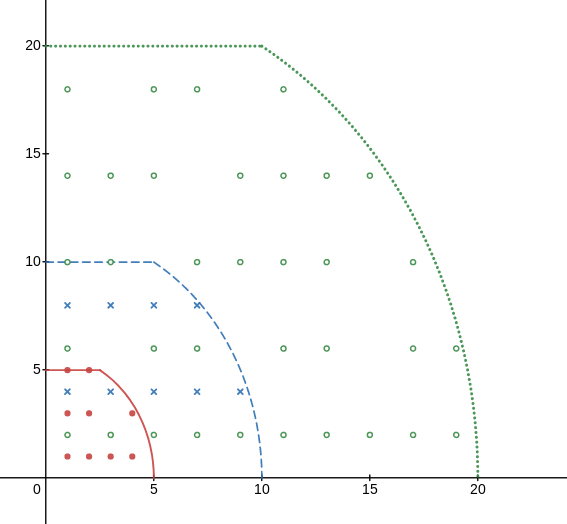
Figure 1. $\mathcal{N}(\phi_{-3}(\mathbf{Q}^{\times}),100)={\color[rgb]{0.78125,0.26953125,0.25390625}9}+{\color[rgb]{0.296875,0.59375,0.34375}35}+{\color[rgb]{0.2578125,0.4921875,0.73046875}9}=53$           

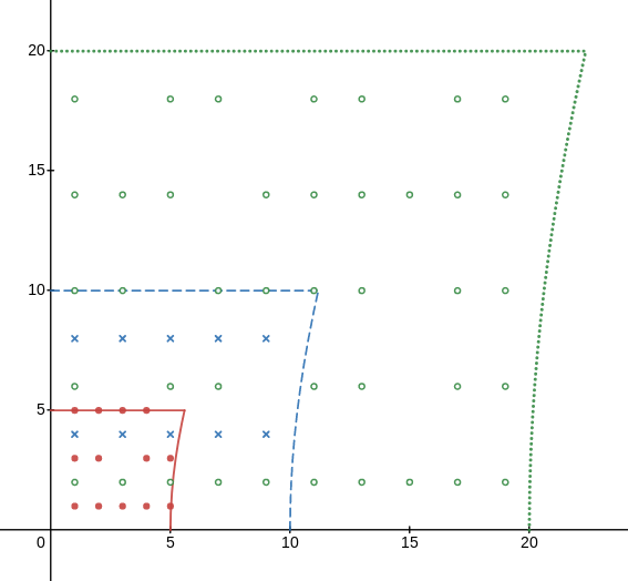
Figure 2. $\mathcal{N}(\phi_{1}(\mathbf{Q}^{\times}),100)={\color[rgb]{0.78125,0.26953125,0.25390625}13}+{\color[rgb]{0.296875,0.59375,0.34375}41}+{\color[rgb]{0.2578125,0.4921875,0.73046875}10}=64$           

Step 3: Analytic number theory. Our final task is to count the number of points in $S_{q,r}$. By Fubini’s theorem,

(8.10) $$\#S_{q,r}=\!\!\sum_{\begin{subarray}{c}b\leqslant\frac{1}{2}\!\sqrt{dX}\\ b\equiv r\,(q)\end{subarray}}\!\!F_{b}\big{(}\tfrac{1}{2}\sqrt{dX+cb^{2}}\big{)}$$

where $F_{b}(Y):=\#\{1\leqslant a\leqslant Y:\gcd(a,b)=1\}$. Appealing to

$$\sum_{k\mid n}\frac{\mu(k)}{k}=\frac{\varphi(n)}{n}$$

we have

$$F_{b}(Y) =\sum_{1\leqslant a\leqslant Y}\sum_{k\mid\gcd(a,b)}\mu(k)$$

$$=\sum_{k\mid b}\mu(k)\sum_{1\leqslant a\leqslant Y,\,k\mid a}1$$

$$=\sum_{k\mid b}\mu(k)\Big{\lfloor}\frac{Y}{k}\Big{\rfloor}$$

$$=Y\sum_{k\mid b}\frac{\mu(k)}{k}-\sum_{k\mid b}\mu(k)\Big{\{}\frac{Y}{k}\Big{\}}$$

whence

$$\Big{\lvert}F_{b}(Y)-Y\frac{\varphi(b)}{b}\Big{\rvert}\leqslant\sum_{k|b}\Big{\lvert}\Big{\{}\frac{Y}{k}\Big{\}}\Big{\rvert}<2^{\omega(b)}.$$

because the sum is supported on the set of primes dividing $b$. It’s well known that $2^{\omega(b)}\leqslant\tau(b)$, the number of divisors of $b$; and by Dirichlet’s theorem,

$$\sum_{b\leqslant Y}\tau(b)\ll Y\log Y.$$

Plugging these into (8.10) yields

$$\#S_{q,r} =\!\!\sum_{\begin{subarray}{c}b\leqslant\frac{1}{2}\!\sqrt{dX}\\ b\equiv r\,(q)\end{subarray}}\!\!\Big{(}\tfrac{1}{2}\sqrt{dX+cb^{2}}\cdot\frac{\varphi(b)}{b}+O(\tau(b))\Big{)}$$

(8.11) $$=\tfrac{1}{2}G_{q,r}\big{(}\tfrac{1}{2}\sqrt{dX}\big{)}+O\big{(}\sqrt{X}\log X\big{)}$$

where

$$G_{q,r}(Y)=\sum_{\begin{subarray}{c}b\leqslant Y\\ b\equiv r\,(q)\end{subarray}}\sqrt{4Y^{2}+cb^{2}}\cdot\frac{\varphi(b)}{b}.$$

It remains to estimate $G_{q,r}$. With an eye to applying Abel summation, we first show that there exist constants $C_{q,r}>0$ such that

(8.12) $$H_{q,r}(Y):=\sum_{\begin{subarray}{c}b\leqslant Y\\ b\equiv r\,(q)\end{subarray}}\!\frac{\varphi(b)}{b}\\ =C_{q,r}Y+O(\log Y).$$

Indeed,

$$H_{q,r}(Y)=\sum_{\begin{subarray}{c}b\leqslant Y\\ b\equiv r\,(q)\end{subarray}}\sum_{k|b}\frac{\mu(k)}{k}=\sum_{k\leqslant Y}\frac{\mu(k)}{k}\#\{1\leqslant b\leqslant Y:k\text{ divides $b$ and }b\equiv r\ (q)\}.$$

The set of $b$’s can be counted using a generalization of the Chinese Remainder Theorem to non-coprime moduli: the system

$$x \equiv r\pmod{n}$$

$$x \equiv s\pmod{m}$$

has a unique solution modulo $\operatorname{lcm}(n,m)$ if and only if $r\equiv s$ (mod $\gcd(n,m)$). Thus

$$\#\{1\leqslant b\leqslant Y:b\equiv 0\ (k)\text{ and }b\equiv r\ (q)\}=[\gcd(k,q)|r]\cdot\Big{\lfloor}\frac{Y}{\operatorname{lcm}(k,q)}\Big{\rfloor}$$

where the Iverson bracket $[P]$ is 0 or 1 according as the statement $P$ is true or false. Writing $a_{k}=\mu(k)\gcd(k,q)[\gcd(k,q)|r]$ it follows that

$$H_{q,r}(Y)=\frac{1}{q}\sum_{k\leqslant Y}\frac{a_{k}}{k^{2}}\cdot Y+O(\log Y)$$

since the error is bounded by the $Y$^th harmonic number. Now, $|a_{k}|\leqslant q$ for all $k$, so

$$\sum_{k\leqslant Y}\frac{a_{k}}{k^{2}}=\sum_{k=1}^{\infty}\frac{a_{k}}{k^{2}}+O(1/Y)$$

and therefore,

$$H_{q,r}(Y)=\underbrace{\frac{1}{q}\sum_{k=1}^{\infty}\frac{a_{k}}{k^{2}}}_{C_{q,r}}\mathbin{\cdot}Y+O(\log Y).$$

We shall also require the exact numerical value of the constant $C_{q,r}$ for our three particular pairs $(q,r)$. The coefficients $a_{k}$ are multiplicative, and a straightforward computation with Euler products supplies the neat formula

(8.13) $$C_{q,r}=\frac{6}{\pi^{2}}\cdot\frac{1}{\varphi(q)}\prod_{p\mid q}\frac{p-[p|r]}{p+1}.$$

Without further ado, let $g(t)=\sqrt{4Y^{2}+ct^{2}}$. Note that

$$g(Y)=\sqrt{4+c}\cdot Y\quad\text{and}\quad g^{\prime}(t)=\frac{ct}{g(t)}.$$

By Abel summation,

$$G_{q,r}(Y)=\sqrt{4+c}\cdot YH_{q,r}(Y)-\int_{1}^{Y}\frac{ctH_{q,r}(t)}{g(t)}\,dt.$$

Using (8.12) we get

$$\sqrt{4+c}\cdot YH_{q,r}(Y)=\sqrt{4+c}\cdot C_{q,r}Y^{2}+O(Y\log Y)$$

while

$$\int_{1}^{Y}\frac{ctH_{q,r}(t)}{g(t)}\,dt=C_{q,r}\int_{1}^{Y}\frac{ct^{2}}{g(t)}\,dt+O\Big{(}\int_{1}^{Y}\frac{t\log(t)}{g(t)}\,dt\Big{)}.$$

Since $Y\geqslant t\geqslant 1$ in the range of integration,

$$g(t)=\sqrt{4Y^{2}+ct^{2}}\geqslant\sqrt{4t^{2}+ct^{2}}=\sqrt{4+c}\cdot t$$

so that

$$\int_{1}^{Y}\frac{t\log t}{g(t)}\,dt\ll\int_{1}^{Y}\log t\ll Y\log Y.$$

For the main term we use the explicit antiderivative

$$\int\frac{ct^{2}}{\sqrt{4Y+ct^{2}}}\,dt=\frac{1}{2}t\sqrt{4Y+ct^{2}}-\frac{2}{\sqrt{|c|}}Y^{2}A\Big{(}\frac{t\sqrt{|c|}}{2Y}\Big{)}$$

where $A(x)=\operatorname{arsinh}(x)$ if $c>0$ and $A(x)=\arcsin(x)$ if $c<0$ (the point is that $A^{\prime}(x)=(1+\operatorname{sgn}(c)x^{2})^{-1/2}$). In either case, $A(x)=x+O(x^{3})$ as $x\to 0$. Since

$$\frac{1}{2}g(1)-\frac{2}{\sqrt{|c|}}Y^{2}A\Big{(}\frac{\sqrt{|c|}}{2Y}\Big{)}=O(Y^{-1})$$

it follows that

(8.14) $$G_{q,r}(Y)=\underbrace{\Big{[}\frac{\sqrt{4+c}}{2}+\frac{2}{\sqrt{|c|}}A\Big{(}\frac{\sqrt{|c|}}{2}\Big{)}\Big{]}}_{\gamma(c)}C_{q,r}Y^{2}+O(Y\log Y).$$

Step 4: Wrap-up. Inserting (8.14) with $Y=\frac{1}{2}\sqrt{dX}$ into (8) yields

$$\#S_{q,r}=\frac{1}{8}\gamma(c)dC_{q,r}X+O(\sqrt{X}\log X).$$

Summing this over $(q,r)\in\{(2,1),(4,2),(4,0)\}$ gives

$$\mathcal{N}(\phi_{c}(\mathbf{Q}^{\times}),X)=\frac{1}{8}\gamma(c)\big{(}C_{2,1}+16C_{4,2}+4C_{4,0}\big{)}X+O(\sqrt{X}\log X)$$

by (8.9). The formula (8.13) implies

$$C_{2,1}=\frac{4}{\pi^{2}}\quad\text{and}\quad C_{4,2}=C_{4,0}=\frac{1}{\pi^{2}}$$

so

$$\mathcal{N}(\phi_{c}(\mathbf{Q}^{\times}),X)=\frac{3}{\pi^{2}}\gamma(c)X+O(\sqrt{X}\log X).$$

Plugging this into (8.7) shows that

$$n_{X}(E^{*})=\frac{3}{\pi^{2}}\big{(}\gamma(1)+\gamma(-3)\big{)}X+O(\sqrt{X}\log X)$$

and Theorem 8.3 follows on evaluating

$$\gamma(1)=\frac{\sqrt{5}}{2}+2\log\frac{1+\sqrt{5}}{2}\quad\text{and}\quad\gamma(-3)=\frac{1}{2}+\frac{2\pi}{3\sqrt{3}}.\qed$$

Remark 8.5.

Every degree-2 rational map with a critical point of period 2 is either totally ramified or else conjugate to a member of the family

$$f_{t}(z)=\frac{t}{z^{2}-z}$$

via a Möbius map moving the critical point, its image, and its non-periodic preimage to $\infty$, 0, and 1 respectively. By Example 7.2, the average number of preperiodic points of this family is 3.

The classification theorem of Canci and Vishkautsan [5] implies that

$$\mathcal{R}(X)\geqslant 2\cdot\mathcal{N}(\psi(\mathbf{Q}),X)+O(X^{2/3}),\qquad\psi(r)=r^{2}-r,$$

with equality if no $f_{t}$ has a cycle longer than 2. (Sketch. The graphs in rows 2, 3, 5, 6, 7 of [5, Table 5.2] are parametrized by rational curves of degrees 3, 2, 4, 6, 6 respectively.) By a computation completely analogous to the one carried out in the proof of Theorem 8.3, and noting that $\psi(r)=\psi(1-r)$, it can be shown that

(8.15) $$\mathcal{N}(\psi(\mathbf{Q}),X)=\frac{3}{\pi^{2}}\left(\frac{\sqrt{5}}{2}+2\log\frac{1+\sqrt{5}}{2}\right)X+O(\sqrt{X}\log X).$$

Figure 3. $\mathcal{N}(\psi(\mathbf{Q}),100)={\color[rgb]{0.4375,0.33203125,0.6875}65}$           

Remark 8.6.

The form of the asymptotics obtained (in particular, the shapes of the constants) is consistent with the following “geometry of numbers” heuristics.

Let $\phi\in\operatorname{Rat}_{e}(\mathbf{Q})$ and pick a lift $f,g$ defined over $\mathbf{Z}$. Since $\phi$ covers its own image,

$$\mathcal{N}(\phi(\mathbf{P}^{1}(\mathbf{Q})),X)=\!\!\sum_{\begin{subarray}{c}P\in\mathbf{P}^{1}(\mathbf{Q})\\ H(\phi(P))\leqslant X\end{subarray}}\!\frac{1}{\#\big{(}\phi^{-1}(\phi(P))\cap\mathbf{P}^{1}(\mathbf{Q})\big{)}}.$$

Put $j=\#{\big{(}\phi^{-1}(\phi(T:1))\cap\mathbf{P}^{1}(\mathbf{Q}(T))\big{)}}$. By Hilbert’s irreducibility theorem, the set

$$\{P\in\mathbf{P}^{1}(\mathbf{Q}):\#\big{(}\phi^{-1}(\phi(P))\cap\mathbf{P}^{1}(\mathbf{Q})\big{)}\neq j\}$$

is thin. From this and standard height estimates it follows that

(8.16) $$\mathcal{N}(\phi(\mathbf{P}^{1}(\mathbf{Q})),X)=\frac{1}{j}\#\{P\in\mathbf{P}^{1}(\mathbf{Q}):H(\phi(P))\leqslant X\}+O(X^{1/e}).$$

Note that if $e=2$ then the error term is actually $O(1)$. The main term is equal to (*)

$$\frac{1}{2j}\sum_{d}\#\{(a,b)\in\mathbf{Z}^{2}_{\mathrm{vis}}:\gcd(f(a,b),g(a,b))=d,\,\max\{|f(a,b)|,|g(a,b)|\}\leqslant dX\}$$

where $\mathbf{Z}_{\mathrm{vis}}=\{(a,b)\in\mathbf{Z}^{2}:\gcd(a,b)=1\}$ is the set of lattice points “visible” from the origin, and the factor of a half accounts for the symmetry $(a:b)=(-a:-b)$ coming from the roots of unity in $\mathbf{Q}$. Note that for any $r>0$, the set

$$\{(x,y)\in\mathbf{R}^{2}:\max\{|f(x,y)|,|g(x,y)|\}\leqslant r\}$$

is precisely the preimage under $\Phi=(f,g)$ of the $\ell_{\infty}$-ball $B(0,r)$. By homogeneity, $\Phi^{-1}(B(0,r))=r^{1/e}\Phi^{-1}(B(0,1))$. Let $D_{\Phi}=\Phi^{-1}(B(0,1))$ and let $\operatorname{vol}(D_{\Phi})$ denote its area. Then a basic principle of the geometry of numbers (see, e.g., [13, Chapter 3, Theorem 5.1]) implies that the number of lattice points in $\Phi^{-1}(B(0,r))$ is

(8.17) $$\#(\mathbf{Z}^{2}\cap r^{1/e}D_{\Phi})=\operatorname{vol}(D_{\Phi})r^{2/e}+O(r^{1/e}).$$

where the $O$-term depends on $\Phi$.

Heuristically, since

$$\#(\mathbf{Z}^{2}\cap B(0,r))=(2\lfloor r\rfloor+1)^{2}\ \text{ and }\ \#(\mathbf{Z}^{2}_{\mathrm{vis}}\cap B(0,r))=2\,\mathcal{N}(\mathbf{P}^{1}(\mathbf{Q}),r),$$

one expects that replacing $\mathbf{Z}^{2}$ by $\mathbf{Z}^{2}_{\mathrm{vis}}$ in (8.17) should introduce a factor of $6/\pi^{2}$ and an error of $O(r^{1/e}\log r)$. By the Chinese Remainder Theorem, further restricting $(a,b)$ to satisfy $\gcd(f(a,b),g(a,b))=d$ should introduce a rational scale factor $C_{d}$ depending on $\Phi$, seeing as

$$d\mid f(a,b)\text{ and }d\mid g(a,b)\iff(a,b)\in\pi_{d}^{-1}\big{(}V(f,g)(\mathbf{Z}/d\mathbf{Z})\big{)}$$

where $\pi_{d}:\mathbf{Z}^{2}_{\mathrm{vis}}\to\mathbf{P}^{1}(\mathbf{Z}/d\mathbf{Z})$ is the reduction map to the projective line over the ring of integers mod $d$. Thus, one expects that each summand in (*) is asymptotically

(8.18) $$\frac{6}{\pi^{2}}C_{d}\operatorname{vol}(D_{\Phi})d^{2/e}X^{2/e}+O(X^{1/e}\log X).$$

As for the number of terms, the elimination property of the resultant implies that $d$ is a divisor of $R_{\Phi}:=\operatorname{Res}(f,g)$. To wit, one can find (by inverting the Sylvester matrix) homogeneous forms $A_{1},\ldots,A_{4}$ in $\mathbf{Z}[f_{e},g_{e},\ldots,f_{0},g_{0}][x,y]$ of degree $e-1$ such that

$$A_{1}f+A_{2}g=R_{\Phi}x^{2e-1}\quad\text{and}\quad A_{3}f+A_{4}g=R_{\Phi}y^{2e-1}.$$

Setting $x=a$ and $y=b$, and noting that $v_{p}(A_{i}(a,b))\geqslant 0$ (as $v_{p}(f,g)\geqslant 0$), yields

$$\min\{v_{p}(f(a,b)),v_{p}(g(a,b))\}\leqslant v_{p}(R_{\Phi})+(2e-1)\min\{v_{p}(a),v_{p}(b)\}$$

for all primes $p$. The l.h.s. is $v_{p}(d)$ and the r.h.s. is $v_{p}(R_{\Phi})$, whence the claim.

Summing (8.18) over all $d$ dividing $R_{\Phi}$, we are thus led to the heuristic formula

(8.19) $$\mathcal{N}(\phi(\mathbf{P}^{1}(\mathbf{Q})),X)=\frac{3}{j\pi^{2}}\operatorname{vol}(D_{\Phi})\!\!\sum_{\ d\mid R_{\Phi}}\!C_{d}\,d^{2/e}X^{2/e}+O(X^{1/e}\log X).$$

For $\Phi(x,y)=(cy^{2}-4x^{2},4y^{2})$ we have $j=e=2$, $\operatorname{vol}(D_{\Phi})=\frac{1}{2}\gamma(c)$, $R_{\Phi}=4^{4}$, and

$$C_{d}=\begin{cases}2/3&d=1,\\ 1/6&d=4\text{ or }16\end{cases}$$

so that $C_{1}+4C_{4}+16C_{16}=4$.

References

- [1] Matthew H. Baker “A finiteness theorem for canonical heights attached to rational maps over function fields” In Journal für die Reine und Angewandte Mathematik 626, 2009, pp. 205–233
- [2] Robert L. Benedetto “Preperiodic points of polynomials over global fields” In Journal für die Reine und Angewandte Mathematik 608, 2007, pp. 123–153
- [3] Robert L. Benedetto “Reduction, Dynamics, and Julia Sets of Rational Functions” In Journal of Number Theory 86, 2001, pp. 175–195
- [4] Pierre Le Boudec and Niki Myrto Mavraki “Arithmetic dynamics of random polynomials” In arXiv, 2021
- [5] Jung Kyu Canci and Solomon Vishkautsan “Quadratic maps with a periodic critical point of period 2” In International Journal of Number Theory 13.6, 2017, pp. 1393–1417
- [6] John R. Doyle and Bjorn Poonen “Gonality of dynatomic curves and strong uniform boundedness of preperiodic points” In Compositio Mathematica 156.4, 2020, pp. 733–743
- [7] S.. Golomb “Powerful Numbers” In The American Mathematical Monthly 77.8, 1970, pp. 848–852
- [8] Robert Grizzard and Joseph Gunther “Slicing the stars: counting algebraic numbers, integers, and units by degree and height” In Algebra & Number Theory 11.6, 2017, pp. 1385–1436
- [9] G.. Hardy and S. Ramanujan “The normal number of prime factors of a number ” In The Quarterly Journal of Pure and Applied Mathematics xlviii, 1917, pp. 76–92
- [10] Benjamin Hutz and Patrick Ingram “On Poonen’s conjecture concerning rational preperiodic points of quadratic maps” In Rocky Mountain Journal of Mathematics 43.1, 2013, pp. 193–204
- [11] Patrick Ingram “Canonical Heights and Preperiodic Points for Certain Weighted Homogeneous Families of Polynomials” In International Mathematics Research Notices 2019.15, 2018, pp. 4859–4879
- [12] Edmund Landau “Einführung in die Elementare und analytische Theorie der algebraischen Zahlen und der Ideale” Providence: AMS Chelsea Publishing, 2005
- [13] Serge Lang “Fundamentals of Diophantine Geometry” New York: Springer-Verlag, 1983
- [14] Alon Levy, Michelle Manes and Bianca Thompson “Uniform bounds for pre-periodic points in families of twists” In Proc. Amer. Math. Soc 142.9, 2014, pp. 3075–3088
- [15] Nicole Looper “The Uniform Boundedness and Dynamical Lang Conjectures for polynomials” In arXiv, 2021
- [16] David Masser and Jeffrey D. Vaaler “Counting Algebraic Numbers with Large Height II” In Trans. Amer. Math. Soc 359.1, 2007, pp. 427–445
- [17] M. Murty and Jeanine Van Order “Counting integral ideals in a number field” In Expositiones Mathematicae 25, 2007, pp. 53–66
- [18] Mateusz Grzegorz Olechnowicz “Preperiodicity in arithmetic dynamics”, 2023
- [19] Bjorn Poonen “The classification of rational preperiodic points of quadratic polynomials over : a refined conjecture” In Mathematische Zeitschrift 228, 1998, pp. 11–29
- [20] Mohammad Sadek “Families of polynomials of every degree with no rational preperiodic points” In Comptes Rendus Mathématique 359.2, 2021, pp. 195–197
- [21] Mohammad Sadek “On rational periodic points of ” In arXiv, 2018
- [22] Stephen Hoel Schanuel “Heights in number fields” In Bulletin de la Société Mathématique de France 107, 1979, pp. 433–449
- [23] Jean-Pierre Serre “Lectures on the Mordell-Weil theorem”, 1989
- [24] Peter Shiu “A Brun-Titchmarsh theorem for multiplicative functions” In Journal für die reine und angewandte Mathematik 313, 1980, pp. 161–170
- [25] Joseph H. Silverman “The Arithmetic of Dynamical Systems”, Graduate Texts in Mathematics 241 New York: Springer, 2007
- [26] Sebastian Troncoso “Bounds for preperiodic points for maps with good reduction” In Journal of Number Theory 181, 2017, pp. 51–72
- [27] Ralph Walde and Paula Russo “Rational Periodic Points of the Quadratic Function ” In The American Mathematical Monthly 101.4, 1994, pp. 318–331