A site-site interaction two-dimensional model with water like structural properties

Abstract

A site-site interaction model is proposed for water in two-dimension, as an alternative to the traditional Mercedes-Benz model. In MB model, water molecules are modeled as 2-dimensional Lennard-Jones disks with three hydrogen bonding arms arranged symmetrically, resembling the Mercedes-Benz logo. The MB model qualitatively predicts both the anomalous properties of pure water and the anomalous solvation thermodynamics of non-polar molecules. One of the features of this earlier model was to have a pair correlation function with first peak for the Lennard-Jones contact distinct of that corresponding to the hydrogen bonding, which is very different from real water which has a single first peak, but a dual peak for the structure factor. The site-site model proposed here reproduces this typical feature of real water, both in real and reciprocal space. It also reproduces several of the known anomalies of real water, such as the density maximum. In addition, because of the screened Coulomb interaction between the sites, the new model appear to exhibit more homogeneity that the MB models and their variants, the latter which is highlighted by a $k=0$ increase of their structure factors. The new model transfers the usual bond order paradigm into a charge order paradigm, enforcing atom-atom interactions over orientational interactions.

¹Laboratoire de Physique Théorique de la Matière Condensée (UMR CNRS 7600), Sorbonne Université, 4 Place Jussieu, F75252, Paris cedex 05, France.

²Faculty of Chemistry and Chemical Technology, University of Ljubljana, Vecna pot 113, 1000 Ljubljana, Slovenia.

1 Introduction

Liquid water, the most abundant liquid and common liquid on Earth, is also the most elusive as far as its numerous anomalous properties are concerned - more than 60 in the sole liquid phase[1, 2]. These anomalous properties are believed to be related to the hydrogen bonding property and tetrahedrality[3, 4], which makes water an associated liquid because of the underlying Hbond “network”[9]. The hydrogen bonding is crucial to understand the behaviour and properties of water and aqueous solutions. Despite extensive theoretical efforts and simulations, how water properties emerge from its molecular structure remains poorly understood. A large number of models of varying complexity have been developed and analysed to model water’s unusual properties, for reviews, see [5, 6]. The key goal of liquid–state statistical thermodynamics is to develop a quantitative theories for water and aqueous solutions. It is generally admitted that theory and simulations have only partly explained how water’s molecular structure leads its density, compressibility, expansion coefficient and heat capacity as functions of temperature and pressure, including its well known anomalies. There have been two main approaches to modeling properties of liquids. One approach is to perform computer simulations of atomically detailed models. These models aim for realistic detail and include variables describing van der Waals and Coulomb interactions, hydrogen bonding, etc. (reviewed in [7]). Such approaches can depend critically on the force–field used in the calculation[8]. However, many properties of water and aqueous solutions can also be captured by simpler models. While the existence and properties of hydrogen bond network have proven quite difficult to characterise both experimentally and theoretically, water thermo-physical properties and structure are usually discussed in terms of the local Hbond and tetrahedral molecular configurations[10, 11]. Related studies has led to many speculations on the possible underlying structure of this liquid, both for pure water[12] and aqueous mixtures[13]. While it is quite difficult to picture three dimension water network, the two-dimension Mercedes-Benz (MB) water model, originally proposed by Ben-Naim in 1971[14, 15], has considerably helped improve this situation, particularly through the numerous studies by Ken Dill and collaborators[16, 17, 18, 19]. These studies has helped consolidating intuitive pictures of water structure and behaviour near hydrophilic and hydrophobic solutes, as described in the review article[5]. The MB model serves as one of the simplest models of an orientationally dependent liquid, so it can serve as a test bed for developing analytical theories. Another important advantage of the MB model, compared to more realistic water models, is that the underlying physical principles can be more readily explored and visualized in two dimensions. The MB model was also extensively studied by analytical methods such as thermodynamic perturbation theory and integral equation theory [17, 20, 21, 22, 23, 24, 25].

Despite these advances, this model has some disadvantages. The MB water model is entirely based on the angular orientation of the 3 hydrogen bonding arms, and because of this it requires supplementary interaction hypothesis in order to be extended to study aqueous mixtures[26, 27], and in particular electrolytes[28, 29]. In addition, it does not have a pair distribution function $g(r)$ which looks like that of real water. Indeed, the pair distribution function of water has very peculiar properties[30] unlike other simple molecular liquids. In particular, the first peak is very narrow and positioned at quite small distance of $r\approx 2.8\mathring{A}$, when the water diameter is $\sigma_{w}\approx 3.1\mathring{A}$. This is a direct consequence of the directionality and strength of the hydrogen bonding. The $g(r)$ of the MB model has 2 peaks instead of one, a first narrow peak which corresponds to hydrogen bonding of the real water, but also a second smaller pre-peak, which corresponds to the water-water direct contact $\sigma_{w}$. This feature is a direct consequence of the choice of setting the Hbonding distance $d_{\mbox{HB}}$ to a value larger than $\sigma_{w}$. This choice insures that the 2D MB model has a density maximum at low temperature[31], in analogy with real water.

In addition to these issues, the 2D representation of water reflects another problem posed by the description of realistic molecular liquids: the orientational versus the atomic representation. A molecule can be represented by it orientation through the set of Euler angles $\vec{\Omega},$or as a set of atoms covalently bonded. This problem is highlighted by the fact that both descriptions are rigorously equivalent at the level of the pair interactions:

$$u(\vec{r},\vec{\Omega}_{1},\vec{\Omega}_{2})=\sum_{i,j}u_{ij}(r_{ij})$$ (1)

where on the lhs the pair interaction is represented in terms of the intermolecular vector $\vec{r}$ between the 2 molecules, and their respective orientations through the set of Euler angles $\vec{\Omega}_{1}$ and $\vec{\Omega}_{2}$, and on the rhs the atomic description with pairs of atoms $i$ and $j$. However, at the level of pair correlations, the two descriptions are not equivalent. The molecular pair correlation function $g(\vec{r},\vec{\Omega}_{1},\vec{\Omega}_{2})$ cannot be expressed in terms of the set of atom-atom pair correlation functions $g_{ij}(r)$, and each type of function provides a different description of the molecular liquid properties. This is the difference between the dipolar or charge-charge description of polar molecular liquids. Interestingly, the 2D MB water model is purely orientational, and has no underlying charged site representation, since it was intentionally built to capture the sole orientational ordering imposed by the hydrogen bonding in real water. We note that the Rose water model introduced subsequently[32, 33] is also an orientational model.

In this context, it is highly desirable to have a site-site equivalent of the MB model, which would allow to introduce other site-site solutes, which would allow a natural site based interaction model, such as in the case of ion-water interaction in a 2D electrolyte representation[28, 29].

In this report, we present a site-site interaction model of water, the SSMB model for site-site Mercedes-Benz model, which is based on a 7 “atoms” representation, with partial charge representation and screened Coulomb interactions, and which provides a convincing alternative to the MB model, while showing a closer structural analogy with real water, in particular in what concerns the $g(r)$. In addition, the site-site representation allows for a straightforward extension of three-dimension solute models in terms of atomic representation, hence permitting to extend and improve the pictorial and intuitive ideas about water and aqueous mixtures.

The principal focus of this paper is the structural features, and not so much the thermodynamical and dynamical properties, which, by construction of the model in analogy with the MB model, should be preserved more or less similarly, albeit for different state parameters such as the temperature and the pressure. With this in mind, the remaining of the paper is as follows. In the next section, the site model is introduced with a brief reminder of the MB model. Section 3 concerns details of the simulations. In Section 4, we first remind the structural properties of the original and modified MB models, before comparing with the structural properties of the site model. In particular, the structure factors are shown, which allows to account for the Fourier representation of the water structure. The final section 5 contains discussions and our conclusions.

2 The site-site model

We first remind the original MB model, as well as a variant of it which we tried in order to merge the Hbond peak and LJ peak into a single one, just as real 3D water.

It is important to note that the model has no net dipole moment. Indeed, in two dimension, it is not possible to have both dipolar ordering and MB-like orientational ordering. However, this is not problematic for the case of ion-water interactions, since the asymmetry of the positive and negative charges allow a natural orientational ordering of the water model around a cation which differs from that around the anion. In that, there is a “circular dipolar” order, instead of the linear dipole of real water, which arise from the difference in orientation of the MB branches and the complementary MB branches.

2.1 The MB model

In the original MB model each particle is represented as two–dimensional disk with Lennard-Jones attraction and three arms arranged as in MB logo, which can form hydrogen bonds between molecules, as illustrated in Fig.1. The angle between arms is 120^∘[14, 16]. The interaction potential between particles $i$ and $j$ is sum of a Lennard–Jones (LJ) term and a hydrogen–bonding (HB) term. The LJ term depends only on the distance between centers of particles while the HB term also on the orientation of each particle:

$$U_{MB}(\vec{X}_{i},\vec{X}_{j})=U_{\mbox{LJ}}(r_{ij})+U_{\mbox{HB}}(\vec{X}_{i},\vec{X}_{j})$$ (2)

where $\overrightarrow{X_{i}}$ is the vector representing the position and orientation of the $i$-th molecule. The Lennard–Jones part of the interaction is calculated in a standard way as:

$$U_{\mbox{LJ}}(r_{ij})=4\epsilon\left[\left(\frac{\sigma}{r_{ij}}\right)^{12}-\left(\frac{\sigma}{r_{ij}}\right)^{6}\right]$$ (3)

where $\sigma$ is the diameter of the LJ disc and $\varepsilon$ is the depth of the LJ potential. The hydrogen bond term is sum of all interactions $U_{HB}^{kl}$ between the arms $k$ and $l$ of molecules $i$ and $j$, respectively

$$U_{\mbox{HB}}(\vec{X}_{i},\vec{X}_{j})=\sum_{k,l=1}^{3}U_{\mbox{HB}}^{kl}(r_{ij},\theta_{i},\theta_{j})$$ (4)

Gaussian functions are used to model arm–arm interactions, which depend on orientation of each molecule as well as distance between molecules

$$U_{\mbox{HB}}^{kl}(r_{ij},\theta_{i},\theta_{j})=\epsilon_{\mbox{HB}}G(r_{ij}-r_{\mbox{HB}})G(\hat{i}_{k}.\hat{r}_{ij}-1)G(\hat{i}_{l}.\hat{r}_{ij}+1)$$ (5)

where $G(x)$ is an unormalized Gaussian function:

$$G(x)=\exp\left(\frac{-x^{2}}{2\sigma^{2}}\right)$$ (6)

$\varepsilon_{HB}$ is the HB energy and $r_{HB}$ is a HB distance. $\hat{r}_{ij}$ is the unit vector along $\overrightarrow{r}_{ij}$ and $\overrightarrow{i}_{k}$ is the unit vector representing the $k$-th arm of the $i$-th particle. Scalar product can be calculated as

$$\hat{i}_{k}.\hat{r}_{ij}=\cos(\theta_{i}+\frac{2\pi}{3}(k-1))$$

where $\theta_{i}$ is the orientation of $i$-th particle. The strongest HB between molecules is formed when arms that form bond are parallel and pointed toward centers of molecules, while distance between centers of molecules is equal to $r_{HB}$. Throughout this paper, we use conventional distance and energy parameters which are the diameter $\sigma$ and the LJ energy $\epsilon_{LJ}$, according to which all distances are expressed in terms $\sigma$ and energies in terms of $\epsilon_{LJ}$.

We used two versions of the MB model, one same as original MB model with the parameter for hydrogen-bond energy, $\varepsilon_{HB}=-10\epsilon_{LJ}$, and for hydrogen-bond length $r_{\mbox{HB}}=1.43\sigma$ as shown in Fig.1(a), and the other called mMB in (b) where use use $\varepsilon_{HB}=-10\epsilon_{LJ}$ and $r_{\mbox{HB}}=\sigma$ .

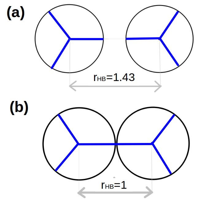
Figure 1: MB water models in Hbonding configuration: (a) Original MB water model, and (b) modified mMB model. All distances are expressed in units of $\sigma$.

One of the problems with the original MB model is that the forcing of optimum Hbonded molecules to be $r_{HB}=1.43\sigma$ apart leads to a very low density water. Higher densities are possible, but with strongly diminished possibility of Hbonded configurations. Although this is not realistic, this original model allows to capture and pictorially illustrate so many features of the real water, that the low density was not seen as a problem. A more realist model is to enforce $r_{HB}=\sigma$, which allows tighter water packing.

2.2 The SSMB model

This model is illustrated in Fig.2. It is made of 6 small “charged” sites and a central LJ site. The small peripheral sites alternatively bear positive (green) and negative(blue) “charges”. These pseudo-charges are used to mimic the original MB branch interactions. They do not correspond to real Coulomb charges per say. Indeed, in this SSMB model, blue negative charges attract each other, while all other charge combinations are Coulomb repulsive. We use a screened Coulomb (Yukawa) interaction.

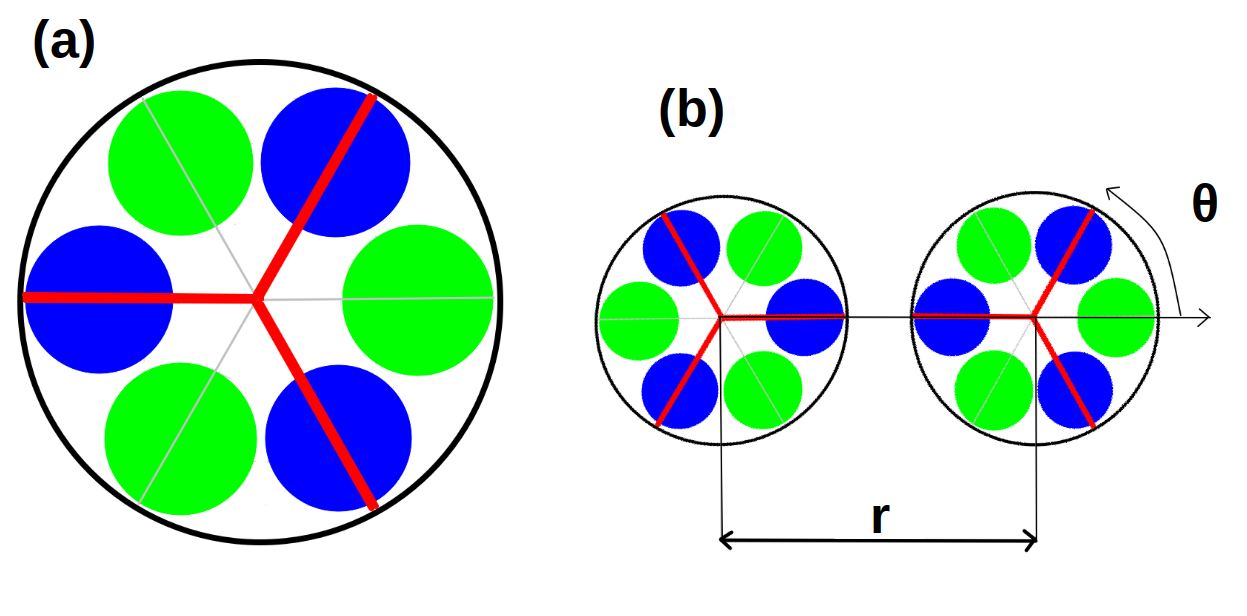
Figure 2: The SSMB 1+6 site water model. (a) The red arms correspond to those of the MB model and are aligned on the blue sites which attract themselves across different molecules. All other color combinations (green-green and blue-green) are repulsive. (b) Two interacting SSMB waters with aligned arms.

The blue charges form the original MB arms (in red in Fig.2), thus preserving the same orientation parameters. However, the total interaction can be now be written as the sum over all pairs of sites:

$$U_{SS}(\vec{X}_{1},\vec{X}_{2})=U_{LJ}(r_{12})+\sum_{i_{1}=1}^{6}\sum_{i_{2}=1}^{6}U_{C}(r_{i_{1}i_{2}})$$ (7)

with the “Coulomb” part having the Yukawa form with a core 12 repulsion (to avoid charge collapse):

$$U_{C}(r_{ab})=\epsilon_{ab}\left(\frac{\sigma_{ab}}{r_{ab}}\right)^{12}+\alpha(a,b)\frac{\exp(-r_{ab}/\kappa_{ab})}{r_{ab}}$$ (8)

where $a$ and $b$ are the (blue/green) site index for each molecule 1 and 2, and the various parameters are as follows. The core repulsive parameters follow the usual Lorentz-Berthelot form, with $\sigma_{ab}=\left(\sigma_{a}+\sigma_{b}\right)/2$ and $\epsilon_{ab}=\sqrt{\epsilon_{a}\epsilon_{b}}$.

The “Coulomb” coefficients $\alpha(a,b)$ are defined as

$$\alpha_{ab}=557s_{ab}Z_{a}Z_{b}$$ (9)

where $Z_{a}$$(Z_{A}>0)$ is the “valence” of site $a$, $s_{ab}$ is the sign of the interaction defined as described above:

$$\begin{array}[]{ccc}s_{blue-blue}&=&-1\\ s_{green-green}&=&+1\\ s_{blue-green}&=&+1\end{array}$$ (10)

This way, blue sites always attract each other, while any other combination lead to a repulsive interaction. The coefficient $557$ represents the “Coulomb” magnitude as defined in our previous works[39, 40]. A model with true Coulomb charges will lead to sites of opposite colors to attract, unlike in the MB model, whereas a model with pure imaginary charges $iZ$ would satisfy like site attractions. However, such model would also imply that green sites would attract each other, thus introducing a severe bias from the MB model spirit. It is for these reasons that the additional coefficient $s_{ab}$ needs to introduced.

The model parameters are then the energy $\epsilon_{a}$, diameter $\sigma_{a},$ Yukawa $\kappa_{a}$ and valence $Z_{a}$ of the blue and green sites, which is $8$ parameters to adjust in order to recover an interaction similar to that of the mMB model.

All the the charged sites are positioned at $d=\sigma/3$ from the center of the molecule. The ($x$,$y$) coordinates of the blue sites are ($d$,$0$), ($-d/2$,$d\sqrt{3}/2$) and ($-d/2$,$-d\sqrt{3}/2$), while the coordinates of the green sites are ($-d$,$0$), ($d/2$,$d\sqrt{3}/2$)) and ($d/2$,$-d\sqrt{3}/2$).

We have selected the parameters as to fit to the closest the mMB model energies for all orientations and distances of 2 water molecules. The following parameters have been used: $\epsilon_{a}=\epsilon_{LJ}/2$, $\sigma_{a}=\sigma/3$, $\kappa_{a}=0.15\sigma$, $Z_{blue}=0.30$, $Z_{green}=0.115$.

2.3 Comparison between the MB, mMB and SSMB models

Fig.3 shows a comparison of the interaction 7 for the original MB model for 2 different values of $r_{HB}$, in a 3-dimensional representation, for fixed orientation of the first water molecule, when the orientation $\theta$ of the second molecule and its distance $r$ to the first one, are both varied. This representation highlights the shifted hydrogen bonding wells for the orientations $\theta=60$, $120$ and $240$, away from then core contact. This shift is thought as an extension of that of the LJ attractive well, positioned at some distance from the core contact.

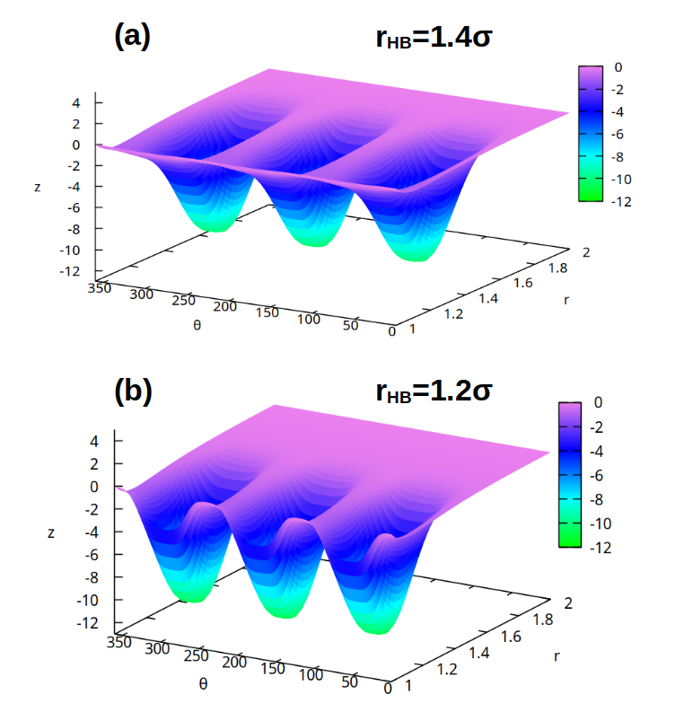
Figure 3: 3-dimension representations of the original MB interaction $U_{MB}(r,\theta_{1}=0,\theta)$ where the water molecule is at fixed orientation $\theta_{1}=0$ , while both the intermolecular distance $r$ and the rotation $\theta_{2}=\theta$ of the second molecule are varied. (a) with the original parameter $r_{HB}=1.4\sigma$, and (b) with the smaller value $r_{HB}=1.2\sigma$, hence showing the influence of this parameter.

Fig.4 shows a similar 3-dimension comparison between the modified mMB model (with $r_{HB}=\sigma$) and the present site-site MB model. The attractive wells are now moved closer to the core $\sigma=1$, as in the real 3D water models. We note that the Gaussian well are more “rounded” than the Yukawa ones, while this second model shows more repulsion between the MB arms.

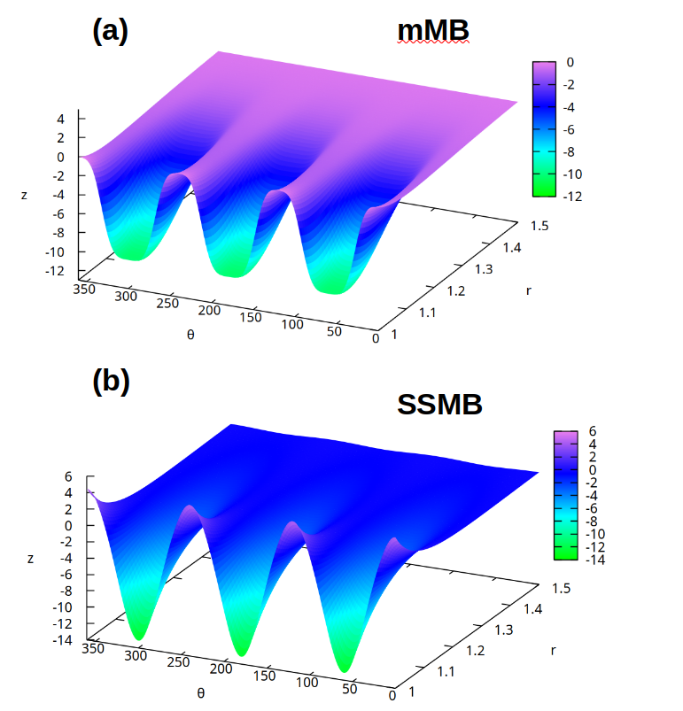
Figure 4: Comparison of the 3-dimension representations of the modified mMB interaction model (a), with $r_{HB}=1.0\sigma$ and the site-site model (b). The conventions are as in Fig.3.

This difference is highlighted in Fig.5, which shows cuts the previous 3D plots, for specific intermolecular distances $r=\sigma$, $1.2\sigma$ and $2\sigma$. The SSMB model is slightly more attractive at the Hbonding angles $\theta=60,120$ and $240$, and more repulsive than the mMB model between the arms, but also at short distance $1.2\sigma$. Since the Gaussian interaction decays faster, one notice the longer range screened-Coulomb type interaction of the Yukawa interaction in the lower panel of Fig.5.

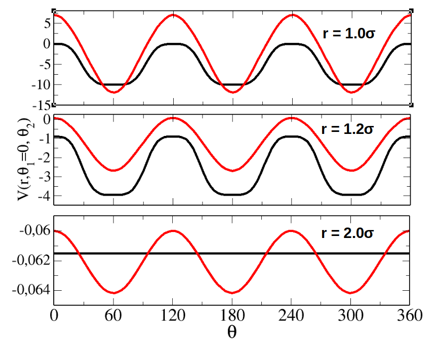
Figure 5: Comparison of the mMB model (black lines) with the SSMB model (red lines), for 3 different intermolecular distances: (top) $r=1.0\sigma$, (middle) $r=1.2\sigma$ and (bottom) $r=2\sigma$.

This long range behaviour should be consistent with the Coulomb nature, when considering other types of molecules, such as ionic species for example, such as those we have considered in our previous works[39, 40].

3 Monte Carlo simulation and technical details

Monte Carlo (MC) simulations with Metropolis algorithm were performed in order to determine thermodynamical properties of the MB model in the isothermal-isobaric (N,p,T) ensemble. Pair correlation functions were computed in the Canonical (N,V,T) ensemble. Periodic boundary conditions and minimum image convention were used to mimic macroscopic system. For NPT ensemble simulations, system sizes from $N=100$ up to $N=400$ water particles were used. This number of particles in 2D is equivalent to $1000$-$8000$ particles in 3D. For NVT ensemble simulations, it was needed to go up to $N=441$ in order to avoid artifacts in the calculated structure factors. The initial positions of particles were randomly chosen in a way where there was no overlap between molecules. A molecule was randomly chosen in each MC step in order to be translated or rotated. On average, each cycle consisted of one rotational and translational attempt per particle and one attempt to change volume of system. First, the system was allowed to equilibrate for minimum of $3\times 10^{4}$ - $10\times 10^{4}$ cycles, which depended on the temperature of the system. After the system was equilibrated, the sampling was performed in 10-20 series, each consisting of minimum $3\times 10^{4}$ cycles. Mechanical properties such as enthalpy and volume were calculated as the statistical averages of these quantities over the course of the simulations [35, 36]. Heat capacity, $C_{p}$, isothermal compressibility, $\kappa_{T}$, and thermal expansion coefficient, $\alpha_{T}$ are computed from the fluctuation formulas of enthalpy, $H$, and volume, $V$ [16].

$$\begin{array}[]{l}c_{p}=\frac{<H^{2}>-<H>^{2}}{NT^{2}}\\ \\ \kappa_{T}=\quad\frac{<V^{2}>-<V>^{2}}{T<V>}\\ \\ \alpha_{T}=\quad\frac{<VH>-<V><H>}{T^{2}<V>}\end{array}$$ (11)

The structure factors $S(k)$ were calculated through the usual Talman transform [37, 38] of the pair correlation function $g(r)$. Since this transform necessitates that the distances are sampled in logarithmic spacing, the regularly spaced $g(r)$ obtained from the computer simulations are interpolated on the logarithmic scale. As a test of this accuracy of the interpolation, we have checked that the $S(k)$ for a simple LJ liquid would be consistent with that obtained from integral equation theories such as Percus-Yevick or Hypernetted-chain equations. This technique was used in our previous works in [39, 40]. Small oscillations often appear in the low-k limit, which arise partly from the Talman technique itself [37], but also from either truncated oscillatory behaviour of $g(r)$ in small boxes. The only remedy is then to simulate larger systems, such that these packing structural oscillations become acceptably small.

4 Results

We first recall the structural features of the original MB model, as well as the modified MB model. The reduced density $\rho$ is defined a for the LJ system by $\rho=(N/S)\sigma^{2},$where N is the number of particles per surface S. This definition differs from that used in the original and subsequent paper, where it is defined with respect to the Hbonding distance $r_{HB}$ as $\rho_{MB}=(N/S)r_{HB}^{2}$ . Similarly, the reduced temperature T is defined in terms of the LJ temperature $T_{LJ}=\epsilon_{LJ}/k_{B}$, where $\epsilon_{LJ}$ is the LJ energy as in Eq.(3) and $k_{B}$ is the Boltzmann constant. The temperature scale is set by $T_{LJ}=1$. This is again different from the original papers where the temperature is scaled by $T_{MB}=\epsilon_{MB}/k_{B}$, where $\epsilon_{MB}$ is the Hbonding energy in Eq.(4).

To summarize, the following scaling correspondence are required to compare the present units with that of previous MB papers: $T=10T_{MB}$, $\rho=0.49\rho_{MB}$, and $r=0.7r_{MB}$.

4.1 Structure of the original MB model

As illustrated in Fig.1, the original MB model with $r_{HB}/\sigma=1$ imposes 2 distinct contact distance, one which is the Hbonding distance at $r=r_{HB}$, and the other the disc-to-disc contact at $r=\sigma$. This is illustrated in Fig.6 through the pair correlation functions for this model, for 2 different densities and 2 different temperatures. The density $\rho=0.8$ correspond to a typical dense liquid, while $\rho=0.6$ is more fluid-like density. In the original MB model, the particles are spaced quite apart because of the large Hbonding distance $r_{HB}=1.4\sigma$. The dual contact distance is quite apparent through the split first peak in the g(r), when the first peak corresponds to the distance $r/\sigma\approx 1$, while the second to $r/\sigma\approx 1.4$. For low density (black curves), it is the Hbond peak which is increased since particles can stay far apart. However, when reaching high packings (red curves), the large Hbonding distance is harder to achieve and it is the first peak which increase. This inversion of the peak increases when reducing the temperature.

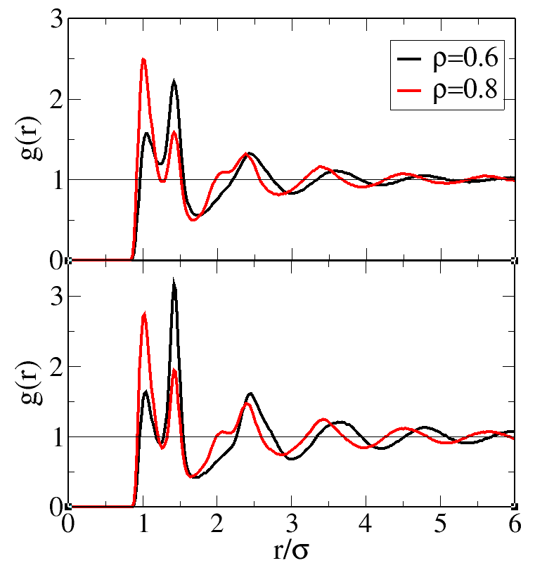
Figure 6: Pair correlation function of the MB water model for 2 different densities and two temperatures $T=3$ (top panel) and $T=2$ (lower panel). Corresponding data was obtained with $N=441$ particles to ensurre proper statistics.

The corresponding structure factors are shown in Fig.7. We note that the large $k$ oscillations are not regular, which arise from the dual peak feature in the $g(r)$. We equally note the raise at $k=0$. Such a raise is usually intepreted in terms of the existence of large density fluctuations. The presence of bonding interactions can also appear as a density fluctuation, since it would increase local heterogeneity. This feature which is also found in real water, but only at low temperatures[41, 42]. It would seem that the MB model over emphasizes such cluster-fluctuations in a wider range of densites and temperatures. We attribute this to the interaction induced heterogeneity in Section 4.5.

Another important feature of this model is the main peak of the structure factor, which do not reflect the dual bonding correlations, as it does for the real water.

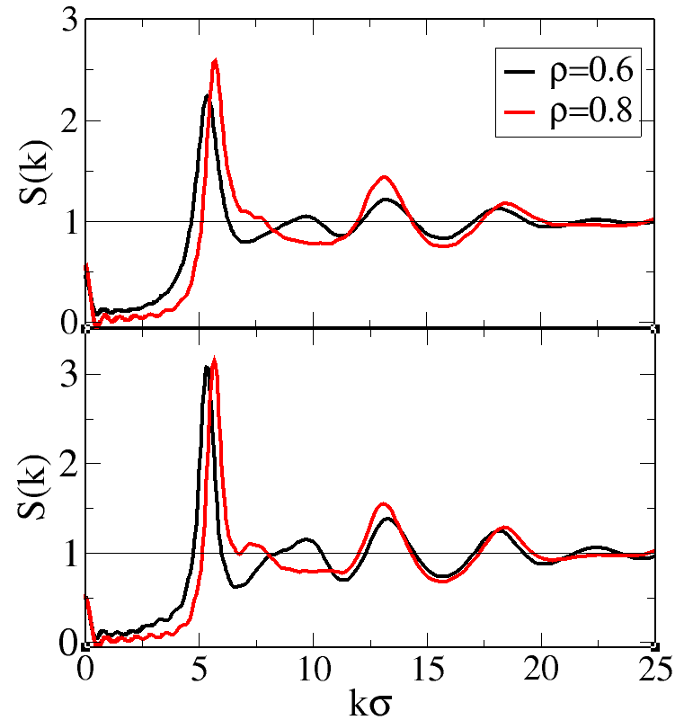
Figure 7: Structure factor of the MB water model for the same state parameters and conventions as in Fig.6

We note that small spurious oscillations, particularly for the low temperature case, which are more pronounced for the lower temperatures and higher densities. Similar artifacts are due to 2D Fourier transform techniques, as discussed in Section 3, and are usually too small to be noticed. However, in the present case, the $k=0$ raise, which is a genuine physical effect due to fluctuations and clustering, amplifies these oscillations to the point they become noticeable. It was necessary to compute $g(r)$ for a larger system of $N=441$ particles, in order to minimize these artifacts, which is an indication of the importance of properly sampling fluctuations for the MB model. These artifacts do not hinder our comprehension of the structure in this model.

4.2 Structure of the modified MB model

The appearance of the dual peak in $g(r)$ for the MB model and its absence in the $S(k)$ main peak are typical feature of this model, and are at variance with that of real water, as illustrated in Fig.8, which shows the oxygen-oxygen pair correlation function and structure factor for the SPC/E model, the latter which is in good agreement with the x-ray experimental data [44, 7]. Both data are taken at ambient conditions for real water. The SPC/E model is one of the popular water models, which represent relatively well most water properties[7]. In the real functions, the split peak is transferred to the main peak of $S(k)$, while the main peak of $g(r)$ is very narrow but with no splitting. Another important feature of the $g(r)$, noted in Ref[[30]] is the abrupt flattening of the large $r$ part of $g(r)$ beyond $r>10\mathring{A}$. This was interpreted as sharp de-correlation of the Hbond beyond $r\approx 10\mathring{A}$, despite the fact that water is quite dense, with $\rho\approx 0.9$.

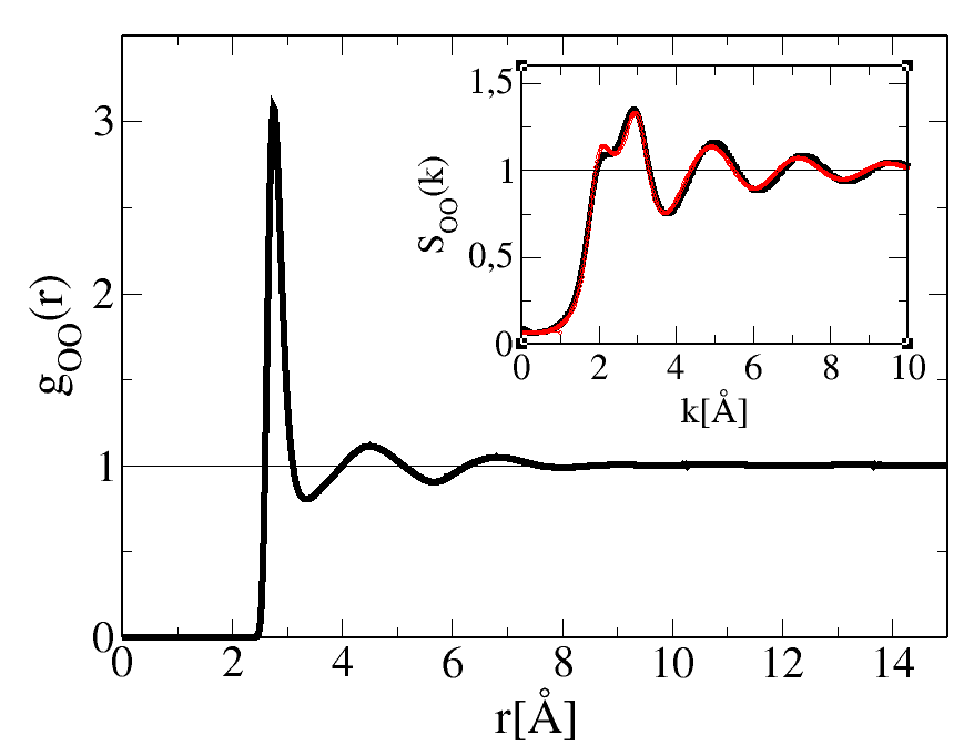
Figure 8: Structure functions of the SPC/E water model. The red curve shows the experimental x-ray structure factor from Ref[44].

In order to recover this feature, we reconsider the MB model, but now allow the shorter Hbonding distance of $r_{HB}/\sigma=1$. We call this modified MB model the mMB model. In this case, the Hbonding distance is very close to the disc-to-disc contact $\sigma$, just like in the real water.

The pair correlation function for this model are shown in Fig.9, while the structure factor are shown in Fig.10, for the same 2 densities and temperature as previously for the MB model. We note that the $g(r)$ are now strikingly similar to that of the real water in Fig.8, with both a sharp first peak and a rapid loss of correlations beyond $r/\sigma\approx 3$. For $\sigma\approx 3\mathring{A}$ for real water, this correspond to nearly the same distance of $10\mathring{A}$ in Fig.8. We also note that there is a much weaker influence of density and temperature than for the MB model, which indicates a system structurally dominated by the Hbonding mechanism.

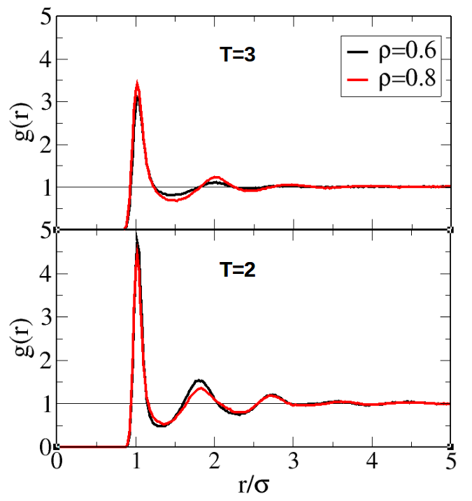
Figure 9: Pair correlation functions of the modified mMB model for $r_{H}=1$, with same state parameters as in Fig.6

The structure factors in Fig.10 equally show interesting features. First of all, for the low temperature $T=2$ case, we note that the main peak develop a weak outer shoulder, exactly as the real water in the inset of Fig.8. This shoulder is absent at the higher temperature, which shows the destruction of Hbonding cluster by heating. Next, we see that the large $k$ behaviour is very regular, which is a direct signature of the packing conditioned by $\sigma$ instead of a dual distance as in the original MB model. Finally, we note the existence of the small $k$-raise very similar to that of the MB model. Since the $k=0$ raise is indicative of density fluctuations, we see that the Hbond clustering can be interpreted as a form of density fluctuations.

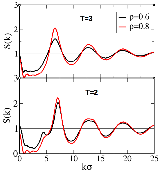
Figure 10: Structure factors of the modified mMB model for r_H=1, with same state parameters as in Fig.6

The additional small wiggles seen in Fig.10, are equally observed in the present case, and are also amplified by the $k=0$ raise for the same reason as explained before for the MB model.

4.3 Structure of the site-site MB model

We now focus on the structural features of the site-site SSMB water model. This is illustrated in Fig.11 for the pair correlation functions $g(r)$, and in Fig.12 for the corresponding structure factors. Due the similarities with the mMB model imposed as illustrated in Fig.4 and Fig.5, we see that the structure functions are also very similar to that of the mMB model. We note, however, that the SSMB has features closer to that the the real water. In particular, we observe a rapid loss of long range correlations, which is a direct consequence of charge ordering, as shown in Ref.[[30]].

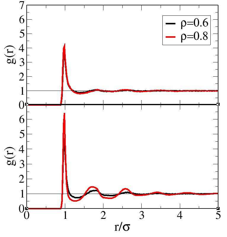
Figure 11: Center-to-center pair correlation functions for the site-site SSMB water model

The similarity with real water is even more striking for the structure factor $S(k)$ in Fig.12, particularly for $T=3$ and $\rho=0.8$. Since the real water data corresponds to ambient conditions, it is tempting to consider these state parameters could equally correspond to 2D ambient conditions. We observe the same dual first peak, which witnesses the dual hydrogen bonding and core contact possibilities for water. At lower temperature, the SSMB model appear more structured that the mMB model.

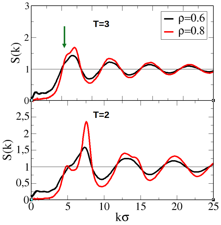
Figure 12: Structure factors of the SSMB model for same state parameters as in Fig.11. The green arrow highlights the shoulder peak similarity with the structure factor of real water (see inset of Fig.8). System size of $N=100$ was used, except for $T=2$ and $\rho=0.8$, for which $N=221$ was found optimal.

We note, however that the $k=0$ behaviour is very different from that of the MB and mMB models, which both showed a rapid raise, suggesting strong density fluctuations, even in equivalent ambient conditions. The SSMB model appears to be closer to the real water, since it shows the absence of such fluctuations. We also note the strong diminution of small-$k$ artifacts, which do not get amplified by the $k=0$ raise, absent from this SSMB model.

4.4 Charge order in the site-site MB model

We now turn toward the “charged” site-site correlations, which should witness site correlations more directly than the center-to-center correlations we analyzed so far. Fig.13 shows a comparison of the density dependence in the upper panel for $T=3$, and in the lower panel a temperature dependence for $\rho=0.6$. It is found that the density dependence of these functions is smaller than their temperature dependence. It corroborates with the intuitive idea that Hbond ordering dominates the particles packing, hence reducing the density dependence, while temperature has a stronger influence in the formation and destruction of the Hbonds.

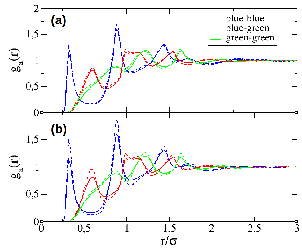
Figure 13: Site-site correlation functions. (a) comparison of the density dependence for $T=3$; full curves for $\rho=0.6$ and dashed curves for $\rho=0.8$. (b) comparison of the temperature dependence for $\rho=0.$6; full curves for $T=3$ and dashed for $T=2$. The blue site correlations are in blue, the green site correlations in green, and cross blue-green correlations in red.

The positions and magnitudes of the various peaks is interesting to analyze. The blue curves have 2 principal peaks, the first one at $r=\sigma/3$, which is the expected blue-blue contact, and the second one at $r\approx\sqrt{(}7)/3$, which is the other blue-blue distance for a typical Hbonding configuration in Fig.2b. Although this second peak is higher than the first one, it represents smaller correlations, since it counts for the 2 possible distances. All other peaks obey similar criteria. These correlation functions provide a strong underlying support for the alignment of the arms supposed to mimic that of the MB model.

Fig.13 equally shows an important property of the SSMB model, which is charge ordering. Indeed, it can be observed that the blue and red curves are in phase opposition, hence witnessing an alternate spatial disposition of the blue and green sites. This is similar to what is seen in the case of charge order in real ionic liquids, both in 3D[43] and 2D [39, 40]. It is interesting that the SSMB model should demonstrate this type of ordering since it does not contain true charges. This is particularly interesting for the perspective of modeling 2D electrolytes with the SSMB water model.

Fig.14 shows the correlation functions from the molecular center to the auxiliary sites, for the case of $T=3$ and $\rho=0.6$. We observe again that the blue and green site correlations are in phase opposition, which is expected as a consequence of phase opposition between the blue and green sites witnessed in Fig.13. The narrower blue peaks witness the strong blue-blue alignment, while the broader green peak witness the more dispersed center to green sites correlations.

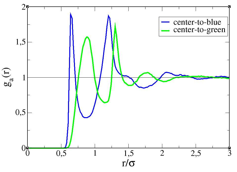
Figure 14: Center to site correlation functions for $T=3$ and $\rho=0.6$, providing another signature of charge ordering (see text).

4.5 Snapshots

Fig.15 shows a comparison of particle configurations (NVT ensemble simulations) between the mMB and SSMB models, for density $\rho=0.8$ and temperature $T=3$. Both configurations appear quite similar, particularly in terms of Hbond ordering. It seems, however, that the SSMB model exhibits visually more homogeneous Hbond ordered particles, which may explain why its structure factor does not exhibit the sharp $k=0$ raise observed for both the MB and mMB models.

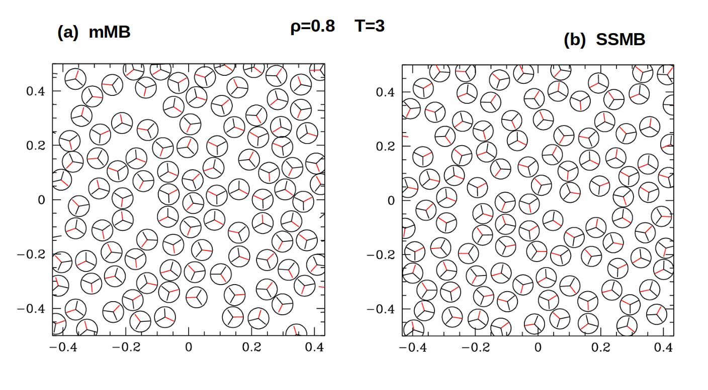
Figure 15: Snapshot comparison between the mMB and the SSMB models, for number of particles N=121. The red arm is assigned such that in the starting configuration, all the red arms point along the y-axis.

The origin of this homogeneity may come from the long ranged Yukawa interaction, while the sharper Gaussian interaction cutoff of the MB and mMB models may favour decorrelation between Hbonded clusters, hence more disordered general distribution.

The influence of this type of disorder may be interesting to study in the context of the presence of solutes and aqueous mixtures in general.

4.6 Thermodynamical anomalies of the SSMB model

The thermodynamic anomalies, as obtained from the SSMB model through Eqs.(11) are shown in Fig.(16). We use the following standard reduced units as: the reduced pressure is $P=p\sigma^{2}/\epsilon_{LJ}$, the reduced compressibility is simply given by $\chi_{T}=S(k=0)$, the reduced thermal expansivity is $\alpha_{T}=\alpha_{T}k_{B}T$ and the reduced heat capacity $C_{P}=C_{P}/k_{B}$ where $k_{B}$ is the Boltzmann constant.

The density maximum is found in (a) around $T\approx 1.6$ for pressure $P\approx 5$ and $T\approx 1.2$ for $P=2$. It is not well defined for $P=5$. The isothermal compressibility in (b) has a clear minimum for $P=2$ and $P=5$, around $T\approx 1.5$. The isobaric heat capacity maximum $C_{P}$ in (d) has also a well defined maximum whose temperature dependence increases with increasing pressures.

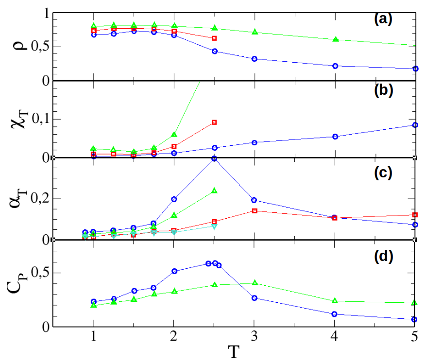
Figure 16: Thermodynamic anomalies of the SSMB water model. (a) density maximum; (b) isothermal compressibility minimum; (c) volume expansivity minimum (see text); (d) isobaric heat capacity maximum. The blue circle is for pressure $P=$1, the red square for $P=$2 and the up triangle for $P=5$. Data for $P=10$ are shown in cyan for $\alpha_{T}$ in (c).

The volume expansivity in (c) does not have a clear minimum, as expected in the low temperature region. A calculation for higher pressure of $P=10$ (cyan curve) does not show any more evidence. In addition, it does not tend to become negative at low temperatures as for the MB model and real water. This is an indication that volume fluctuations and entropy fluctuation remain correlated as $T$ is decreased, instead of becoming anti-correlated as in the case of real water. It is difficult to say if this is a flaw of the SSMB model, since it is not obvious how dimensional reduction, while keeping water-like spatial structure, should affect volume and entropy correlations. This point remains to be explored further. Since the SSMB model does not have the same high density fluctuation at $k=0$ as the MB and mMB models, the absence of expansivity anomaly could be related this property. Indeed, as commented above, the higher spatial homogeneity of the SSMB model, compared with that of the MB model, would imply a lower entropy, hence a higher coupling between volume and entropy fluctuations, at the origin of the absence of anomaly in the expansivity. In any case, it is interesting that this SSMB model should have only some of the water anomalies, but not all. It indicates that dimensional aspects could play an important role. If this is true, then it would imply that, for real water, these anomalies are not necessarily interrelated and could not depend solely on Hbond properties.

4.7 Low temperature phases

Fig.17 shows the type of the low temperature $T=0.9$ amorphous ice that are found for the SSMB. Larges patches of Hbond connected particles are observed at both low and high pressure. But no perfect hexagonal crystal is found. We recall that the MB model crystallises in a perfect hexagonal crystal[16]. It should be reminded that hard discs crystalline phases present alignment distortions, which are generated by the density fluctuations in 2D being larger than in 3D, thus avoiding perfect crystals in 2 dimensions, which is the reason why the solid-liquid melting transition is not first order, but second order with an intermediate Kosterlitz-Thouless phase[47, 48]. The dimensionality plays an important role in phase transitions, and it can be rigorously shown than continuous transitions (unlike that in the Ising model) such as the XY model and Heinsenberg model, are impossible in 2D[49]. The liquid-solid transition in 2D is itself controversial [50].

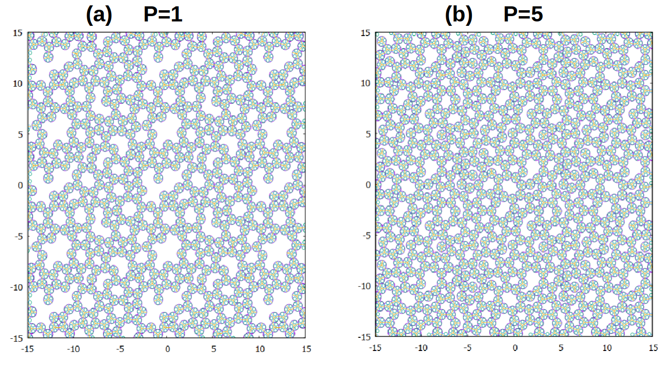
Figure 17: Low temperature amorphous ice phases of the SSMB water model, for T=0.9 and for 2 different pressures.

In this context, by allowing core contact, the MBSS model meets some of these problems common to 2D spherical core interactions. It is then not so surprising that this model does not exhibit a perfect hexagonal crystal. The snapshots of Fig.17 show several clusters of hydrogen bonded pentamer, hexamers, up to disorted octamers. The denser phase for $P=5$ equally shows flattened high order $n$-mers. It does not seem surprising that a realistic 2D water model may not have a perfect crystalline phase.

5 Discussion and Conclusion

We have introduced a site-site two-dimensional water model, named SSMB model, as an alternative to the usual MB model. We have showed that this new model transfers the dual Hbond / core contact paradigm of water, from real space into reciprocal space, in agreement with the real water model. This is an important feature to note, since it is generally advertised that water has this dual order, such as for instance in the Franks water model[45] , implicitly implying an order in real space. The specificity of the water structure has been debated several times[42] , and more recently in the context of the water second critical point[46], which would be related to a phase separation between disordered and Hbond ordered 2 liquids, albeit in metastable conditions. It is not obvious that such issues would be relevant to two-dimensional water models. The MB model has been very successful in allowing to visually illustrate in 2 dimensions many of the water anomalies and specificity in the context of mixing. Although the present work is specifically focused on highlighting the structural aspects of the 2D water models, it would be interesting to examine a site-site version of the MB models extended to various solutes, such as alcohols and ionic species, part of the project prospective which is being currently pursued.

References

- [1] P.Ball, Nature 452, 291 (2008)
- [2] M. Chaplin, water structure and science, https://water.lsbu.ac.uk/water/water_structure_science.html
- [3] J. E. Errington and P. G. Debenedetti, Nature 409, 318 (2001)
- [4] K. Amann-Winkel, M.-C. Bellissent-Funel, L. E. Bove, T. Loerting, A. Nilsson, A. Paciaroni, D. Schlesinger, and L. Skinner, Chem. Rev. 116, 13, 7570 (2016)
- [5] E. Brini, C. J. Fennell, M. Fernandez-Serra, B. Hribar-Lee, M. Luksic, and K. A. Dill, How Water?s Properties Are Encoded in Its Molecular Structure and Energies, Chem. Rev., 2017, 117, 12385-12414.
- [6] P. Gallo, K. Amann-Winkel, C. A. Angell, M. A. Anisimov, F. Caupin, C. Chakravarty, E. Lascaris, T. Loerting, A. Z. Panagiotopoulos, J. Russo, J. A. Sellberg, H. E. Stanley, H. Tanaka, C. Vega, L. Xu and L. G. M. Pettersson, Water: A Tale of Two Liquids, Chem. Rev., 2016, 116, 7463-7500.
- [7] B. Guillot, J. Mol. Liq. 101, 219 (2002).
- [8] J-C. Soetens, C. Millot, C. Chipot, G. Jansen, J. G. Angyán and B. Maigret, J. Phys. Chem. B 101, 10910 (1997).
- [9] J. D. Bernal, and R. H. Fowler, . J. Chem. Phys. 1, 515 (1993).
- [10] F. H. Stillinger, and T. A. Weber, J. Phys. Chem. 87, 2833 (1983).
- [11] H. E. Stanley, S. V. Buldyrev, O. Mishima, M. R. Sadr-Lahijany, A. Scala and F. W. Starr, J. Phys. Cond. Mat. 12, A403 (2000)
- [12] S. D. Overduin and G. N. Patey, J. Phys. Chem. B. 116, 12014 (2012)
- [13] F. F. Purdon and V. W. Slater, Aqueous solution and the phase diagram, Ed. Edward Arnold (London, 1946)
- [14] A. Ben–Naim, Statistical Mechanics of ?Waterlike? Particles in Two Dimensions. I. Physical Model and Application of the Percus?Yevick Equation, J. Chem. Phys. 54, 3682 (1971).
- [15] A. Ben–Naim, Statistical mechanics of water-like particles in two-dimensions, Mol. Phys. 24, 705 (1972).
- [16] K. A. T. Silverstein, A. D. J. Haymet and K. A. Dill, J. Am. Chem. Soc. 120, 3166 (1998).
- [17] T. Urbič, V. Vlachy, Y. V. Kalyuzhnyi, N. T. Southall, and K. A. Dill, J. Chem. Phys. , 112, 2843 (2000).
- [18] T. M. Truskett, and K. A. Dill, . J. Chem. Phys. , 117, 5101 (2002).
- [19] M. Lukşič , T. Urbic, B. Hribar-Lee, and K. A. Dill, J. Phys. Chem. B , 116, 6177 (2012).
- [20] T. Urbic, V. Vlachy, Yu. V. Kalyuzhnyi, N. T. Southall and K. A. Dill, J. Chem. Phys., 2000, 112, 2843-2848.
- [21] T. Urbic, V. Vlachy, Yu. V. Kalyuzhnyi and K. A. Dill, J. Chem. Phys., 2003, 118, 5516-5525.
- [22] T. Urbic, V. Vlachy, O. Pizio, K. A. Dill, J. Mol. Liq., 2007, 112, 71-80.
- [23] T. Urbic, V. Vlachy, Yu. V. Kalyuzhnyi and K. A. Dill, J. Chem. Phys., 2007, 127, 174511.
- [24] T. Urbic, V. Vlachy, Yu. V. Kalyuzhnyi and K. A. Dill, J. Chem. Phys., 2007, 127, 174505.
- [25] T. Urbic and M. F. Holovko, J. Chem. Phys., 2011, 135, 134706.
- [26] Y. Kataoka, J. Chem. Phys. 80, 4470 (1984)
- [27] M. Peyrard, Phys. Rev. E 64, 011109 (2001)
- [28] B. Hribar, N. T. Southall, V. Vlachy, and K. A. Dill, J. Am. Soc. 124, 12302 (2002)
- [29] J. Aupic and T. Urbic, J. Chem. Phys. 140, 184509 (2014).
- [30] A. Perera, Mol. Phys. 109, 2433 (2011)
- [31] T. Urbic and K. A. Dill, Phys. Rev. E 98, 032116 (2018)
- [32] C. H. Williamson, J. R. Hall, and C. J. Fennell, J. Mol. Liq. 228, 11 (2017)
- [33] P. Ogrin and T. Urbic, J. Mol. Liq. 367, 120351 (2022)
- [34] E. Brini, C. J. Fennell, M. Fernandez-Serra, B. Hribar-Lee, M.Lukšič, and Ken A. Dill, Chem. Rev. 117, 12385 (2017)
- [35] J. P. Hansen and I. R. McDonald,Theory of Simple Liquids (Academic, London, 1986).
- [36] D. Frenkel and B. Smit, Molecular simulation: From Algorithms to Applications, (Academic Press, New York, 2000).
- [37] J. D. Talman, J. Comput. Phys. 29, 35 (1978)
- [38] P. G. Ferreira, A. Perera, M. Moreau, and M. M. Telo da Gama, J. Chem. Phys. 95, 7591 (1991)
- [39] A. Perera and T. Urbic, Physica A 495, 393 (2018)
- [40] A. Perera and T. Urbic, J. Mol. Liq. 265, 307 (2018)
- [41] L. Bosio and J. Teixeira, Phys. Rev. Lett., 46, 597 (1981)
- [42] G. N. I. Clark, G. L. Hura, J. Teixeira, A. K. Soper and T. Head-Gordon, Proc. Nat. Am. Soc. 107, 14003 (2010)
- [43] A. Perera and R. Mazighi, J. Mol. Liq. 210, 243 (2015)
- [44] L. B. Skinner and C. J. Benmore, J. Chem. Phys. 138, 074506 (2013).
- [45] Franks, F. Water: A Comprehensive Treatise. Volume 1. The Physics and Physical Chemistry of Water; Plenum Press: 1972.
- [46] F. Hirata, Condensed Matter Physics, 25, 23601 (2022)
- [47] B. I. Halperin and D. E. Nelson, Phys. Rev. Lett. 41, 519 (1978)
- [48] J. Frölich and C. Pfister, Commun. Math. 81, 277 (1981)
- [49] N. D. Mermin and H. Wagner, Phys. Rev. Lett. 17, 1133 (1966)
- [50] K. J. Strandburg, Rev. Mod. Phys. 60, 161 (1988)