MOSAIC: Masked Optimisation with Selective Attention for Image Reconstruction

Abstract

Compressive sensing (CS) reconstructs images from sub-Nyquist measurements by solving a sparsity-regularized inverse problem. Traditional CS solvers use iterative optimizers with hand crafted sparsifiers, while early data-driven methods directly learn an inverse mapping from the low-dimensional measurement space to the original image space. The latter outperforms the former, but is restrictive to a pre-defined measurement domain. More recent, deep unrolling methods combine traditional proximal gradient methods and data-driven approaches to iteratively refine an image approximation. To achieve higher accuracy, it has also been suggested to learn both the sampling matrix, and the choice of measurement vectors adaptively. Contrary to the current trend, in this work we hypothesize that a general inverse mapping from a random set of compressed measurements to the image domain exists for a given measurement basis, and can be learned. Such a model is single-shot, non-restrictive and does not parametrize the sampling process. To this end, we propose MOSAIC, a novel compressive sensing framework to reconstruct images given any random selection of measurements, sampled using a fixed basis. Motivated by the uneven distribution of information across measurements, MOSAIC incorporates an embedding technique to efficiently apply attention mechanisms on an encoded sequence of measurements, while dispensing the need to use unrolled deep networks. A range of experiments validate our proposed architecture as a promising alternative for existing CS reconstruction methods, by achieving the state-of-the-art for metrics of reconstruction accuracy on standard datasets.

1 Introduction

Compressive sensing (CS) has advanced signal processing and data acquisition by enabling accurate signal recovery from highly under-sampled measurements, with numerous applications in imaging, speech/audio processing, and communication systems [33, 31]. The typical CS formalism for imaging employs a sampling matrix, $\mathbf{A}_{m\times n}$, to compressively measure an image signal $\mathbf{x}\in\mathbb{R}^{n}$ as a linear projection $\mathbf{y}=\mathbf{A}\mathbf{x}(m\ll n)$. Given $\mathbf{y}\in\mathbb{R}^{m}$, the subsequent reconstruction model should solve an ill-posed inverse problem to reconstruct the image $\mathbf{\hat{x}}\in\mathbb{R}^{n}$. The seminal works of Donoho [11] and Candes et al. [5] inspired reconstruction algorithms [3, 4, 10] with theoretical guarantees. These methods employ a structural prior $\mathcal{R}(.)$ with a regularization parameter $\lambda$ to form an optimization objective:

$$\underset{\mathbf{x}}{\operatorname{argmin}}\>||\mathbf{A}\mathbf{x}-y||_{2}^{2}+\lambda\mathcal{R}(\mathbf{x}).$$ (1)

Consequently, projected gradient methods [14] have been widely explored which iteratively approximate better reconstructions. These algorithms have a gradient update step to form a residual $\mathbf{\hat{x}}_{k}-\alpha\nabla f(\mathbf{\hat{x}}_{k})$, after which the updated residual is projected back on to a convex set including $\mathbf{x}$.

$$\hat{\mathbf{x}}_{k+1}=\operatorname{P}_{\lambda\mathcal{R}}\left(\hat{\mathbf{x}}_{k}-\alpha\nabla f(\mathbf{\hat{x}}_{k})\right);\quad f(\mathbf{\hat{x}})=||\mathbf{A}\mathbf{\hat{x}}-y||_{2}^{2},$$ (2)

Here $\hat{\mathbf{x}}_{k}$ and $\hat{\mathbf{x}}_{k+1}$ are the signal estimates at iterations $k$ and $k+1$, respectively. $\operatorname{P}_{\lambda\mathcal{R}}$ is the projection operator, parametrized by $\lambda$ and the choice of $\mathcal{R}$. Inevitably, these "traditional" iterative algorithms were replaced with deep learning models to achieve faster inference and higher accuracy by parametrizing terms of equation (2) into learnable weights with a limited number of iterations. They achieve state-of-the-art reconstruction accuracy for standard image datasets, while having the added advantage of requiring only a single forward pass step at inference. In line with exploiting priors of natural images, it is worth noting that natural images have well-exploited structures in some spectral decompositions such as in the frequency domain  [39, 17]. This inherent structure creates a pattern, with each frequency carrying a different information content. We could extend this idea to compressive sensing, when each measurement vector (row $A_{i}$) of the sampling matrix $\mathbf{A}$ is structured such that it corresponds to a different basis frequency that spans the image space. Therefore, each measurement would correspond to sampling at a certain frequency, and given $\mathbf{y}_{m\times 1}$, it is possible to consider $(y_{i},A_{i})$ pairs for $1\leq i\leq m$, as known priors for the reconstruction objective. However, structural priors may not be sufficient to solve an ill-posed inverse problem with high accuracy.

An interesting way to approach CS reconstruction, is to convert it to a ‘measurement filling problem’ similar to that of sentence completion in natural language processing (NLP) [9]. Drawing intuitions from attention-based models in NLP, a potential approach is to employ attention in the measurement space, so that more salient measurements are given more attention. Nevertheless, a crucial challenge is to identify and encode the maximum amount of information from any random set of measurements. While significant progress has been made in compressive sensing, we find that many data driven methods parametrize the sampling process, restricting it to a learnt $\mathbf{A}$.

In this context, we present an attention-based framework for applying CS-specific inductive biases for a deep CS model, for a fixed measurement basis. Specifically, our contributions are as follows:

1. We propose a novel approach for reconstruction of compressively sensed images, exploiting the structure of an orthogonal sampling basis, while dispensing the need for deep unrolling.

2. We present "MOSAIC"; Masked Optimisation with Selective Attention for Image Reconstruction; an end-to-end trainable deep reconstruction model that is not restricted to a learnt sampling process.

3. We demonstrate the effectiveness of "MOSAIC" on compressive sensing, achieving significant improvements in PSNR and SSIM over previous state-of-the-art methods on benchmark datasets, as well as a qualitative review.

2 Related Work

2.1 Projection-based Deep Unrolling

The first family of deep CS reconstruction used black-box CNN models [23, 36, 37]. However, these were lacking interpretability, and were restricted to the specific learnt sampling matrix. Inspired by sparse dictionary encoding algorithms such as Iterative Shrinkage and Thresholding Algorithm (ISTA) [8], the next generation of deep models unroll iterative algorithms such as equation (2) to a series of blocks [47, 27, 43]. To various degrees, these ‘deep unrolling’ models rely on the guarantees of projected gradient methods to form their inductive bias while striving for some level of interpretability. This translates to finding a sweet spot between an inductive bias, and model flexibility, by the conversion of certain parameters to learnable weights. The latest approaches [44, 48, 35, 7], however, only use CS recovery algorithms as inspiration for the model architecture. For example, ISTA-Net++ [44], uses CNNs, while the more recent TransCS [35] uses a hybrid of transformers and CNNs to model the parametrized projection and gradient update step. As an underlying pattern, these models learn an embedding from an image, update a gradient step in the embedding-space, and project back to image-space resembling a deep autoencoder [19]. The reconstruction path is a stack of such autoencoders, progressively refining/denoising $\mathbf{\hat{x}}$, with $\Phi$ and $\mathbf{y}$ acting as priors. However, we notice that these methods update model weights through the gradient of the residual norm $||\Phi\mathbf{\hat{x}}-\mathbf{y}||_{2}$, and that there is no separate treatment for each measurement $\mathbf{y}_{i}$ of $\mathbf{y}$.

2.2 Attention for Image Reconstruction

Masked image modeling is a technique that utilizes images that have been corrupted by masking to learn useful representations. Pioneered with stacked autoencoders [40] using convolutional neural networks (CNNs), while numerous methods [2, 18, 42] have employed the mask-word approach derived from natural language processing (NLP) to randomly obscure image patches within the spatial domain through the utilization of vision transformers [12, 25]. Recent methods incorporating masked autoencoders [18], have shown great promise in similar image processing tasks [46, 16], where they efficiently extract spatial features that are representative of the original data. Learning through autoencoders is a challenge in CS, since the measurement $\mathbf{y}$ itself is low dimensional. Therefore, we propose a structured method of expanding the dimensionality of $\mathbf{y}$, that would enable masked learning in an embedding-space.

2.3 Representation Learning from Transformed Domains

Studies on how image details are represented in frequency space have been extensively studied [29, 30], to show that the phase component of a signal in the frequency domain captures high-level semantics, while the amplitude component preserves low-level statistics. This has motivated deep learning methods to incorporate methods to use transformations such as discrete cosine transform (DCT) [24] and discrete Fourier transform (DFT) [34] to learn image features for subsequent downstream tasks. With the success of masked approaches for visual pretraining, [41] employs masked learning in DFT domain, to learn image features in a self-supervised setting. However, as the transformations in CS are ill-posed, the challenge is to solve for an inverse transformation. Therefore, learning features in the measured space is not as straightforward as existing approaches. Furthermore, the existence on the spectral bias of neural networks towards low frequency information [32, 13] has motivated careful design of deep networks for tasks that are more reliant on high frequency information [28]. Drawing parallels onto the measurement domain, we address these concerns with a measurement embedding scheme, which facilitates masked learning through a mapping into higher dimensions.

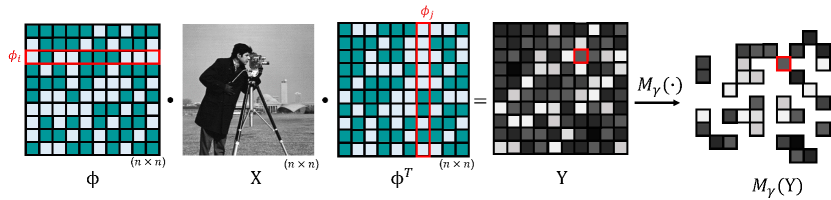
Figure 1: The proposed sampling scheme for compressive sensing of a 2D image: A uniform random sampling from a set of possible measurements $\mathbf{Y}$, is modelled as a uniform random masking $\mathit{M}$ with a compression factor $\gamma$

3 Method

Let $\mathbf{X}_{\sqrt{n}\times\sqrt{n}}$ be the image signal, with pixels values $x_{i,j}\in\mathbb{R}$, at pixel locations $\left(i,j\right)\in S=\left\{\left(i^{\prime},j^{\prime}\right)\in\mathbb{Z}^{2}\ \right|\ 1\leq i\prime,j\prime\leq\sqrt{n}\}$. Here $n=\|\mathbf{X}\|_{0}$ is the number of pixels in the image. Select the transformation matrix $\Phi_{\sqrt{n}\times\sqrt{n}}$ such that a well-posed measurement $\mathbf{Y}_{\sqrt{n}\times\sqrt{n}}$ with entries $y_{i,j}\in\mathbb{R}$ is given by (3), and depicted in Figure 1.

$$\mathbf{Y}_{\sqrt{n}\times\sqrt{n}}=(\Phi\thickspace\mathbf{X}\thickspace\Phi^{T})/k;\quad k\mathbf{I}_{n}=\Phi\Phi^{T}.$$ (3)

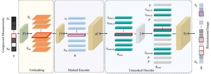
Figure 2: The proposed pipeline for reconstruction: Each sampled measurement $y_{i,j}$ is first projected to a higher dimensional $\mathbf{E}_{i,j}$ by exploiting the structure of sampling matrix $\Phi$. The masked encoder $g(.)$ maps these embeddings which are treated as a sequence of length $m$. In the decoder $h(.)$, the masked embeddings $\mathbf{z}_{enc}$ are padded with placeholer $\mathbf{p}$, and transformed to predict $\hat{\mathbf{x}}\in\mathbb{R}^{n}$. Here, $f(.)$ encodes the handcrafted embeddings into latents $\mathbf{z}$, while $g(.)$ and $h(.)$ are self-attention layers.

From equation (3), $\forall\left(i,j\right)\in S$, for $\mathbf{\phi_{i}},\mathbf{\phi_{j}}$ rows of $\mathbf{\Phi}$, we can write

$$y_{i,j}=\frac{\mathbf{\phi_{i}}\thickspace\mathbf{X}\thickspace\mathbf{\phi}^{T}_{j}}{k}.$$ (4)

Furthermore, note the resemblance of the following decomposition, to a spectral decomposition of $\mathbf{X}$, where a one-to-one mapping exists between the choice of measurement basis vectors $(\mathbf{\phi_{i}},\phi_{j})$, and the measurement value $y_{i,j}$.

$$\mathbf{X}=k\ \sum_{i=1}^{\sqrt{n}}\sum_{j=1}^{\sqrt{n}}\mathbf{\phi_{i}}^{T}y_{i,j}\mathbf{\phi_{j}}.$$ (5)

Compressive sensing: As shown in equation (4), all measurements are indexed by $\left(i,j\right)$ pairs and the set of all measurement indices $S$ has a cardinality, $\left|S\right|=n$. To compressively sample $\mathbf{X}$ we randomly select a subset of $m$ measurements with indices in $S_{C}\subset S\text{ where}\left|S_{C}\right|=m$, following a uniform distribution. The uniform distribution ensures that each measurement has equal weight and minimizes potential sampling biases. Now we can define the compression factor $\gamma$ as,

$$\gamma=\frac{m}{n}<1.$$ (6)

Embedding: Next, using the structure of $\Phi$, we embed each measurement $y_{i,j}$, for $\left(i,j\right)\in S_{C}$, as follows,

$$\mathbf{E}_{i,j}=\mathbf{\phi_{i}}^{T}y_{i,j}\mathbf{\phi_{j}}.$$ (7)

This facilitates the decomposition of the measurements, generating a high dimensional representation of the sampled measurements that can be fed to the subsequent model. Having a high dimensional input alleviates possible spectral biases of the model as motivated by [32].

Each $E_{i,j}$ is then further embedded using a learnable embedding $T(.)$ and positional encoded using a positional embedding $Pos\left(.\right)$ to get the final embedding $\mathbf{z}_{i,j}$ as,

$$\mathbf{z}_{i,j}=f(\mathbf{E}_{i,j},(i,j))=T(\mathbf{E}_{i,j})+Pos(i,j).$$ (8)

Masked encoder: Similar to the original MAE work [18] our positional embedding, $Pos\left(.\right)$ , preserves the original location of the measurement $y_{i,j}$ in $\mathbf{Y}_{\sqrt{n}\times\sqrt{n}}$. Thus, we think about the sampling process as a “masking” operation on $\mathbf{Y}_{\sqrt{n}\times\sqrt{n}}$. Here, $y_{i,j}$’s with $\left(i,j\right)\in S_{C}$ are unmasked measurements while ones with $\left(i,j\right)\in{S-S_{C}}$ are masked.

Next, we treat $\mathbf{z}_{i,j}$’s as an $m$ element sequence, $\mathbf{z}$, such that a given $\mathbf{z}_{i,j}$’s index $k\in\left\{k^{\prime}\in\mathbf{Z}\right|\ 1\leq k^{\prime}\leq m\}$ in the sequence is given by the sorting operator on $S_{C}$ as,

$$k=sort\left(\ \left(i,j\right)\ \right|\ S_{C}\ ).$$ (9)

Then the sequence $\mathbf{z}$ can be written as,

$$\mathbf{z}=(\mathbf{z_{1}},\mathbf{z_{2}},...,\mathbf{z_{k}},...,\mathbf{z_{m}}),$$ (10)

where $\mathbf{z_{i,j}}$ is the same as $\mathbf{z}_{sort\left(\ \left(i,j\right)\ \right|\ S_{C}\ )}$.

We employ an asymmetric design as outlined in Figure 2 inspired by [18] in that it differs from classical encoder-decoder designs. Specifically, the encoder $g(.)$ operates on a sequence of measurement latents ${\mathbf{z}_{k}}$’s, while the decoder aims to reconstruct the full image that was measured, in the pixel domain. As such, we encode $\mathbf{z}$ using the learnable encoder $g(.)$, to get $\mathbf{z}_{enc}=g(\mathbf{z})$.

Unmasked decoder: Following the asymmetric design, our decoder, $h(.)$, takes an $n$ element sequence $\mathbf{z}_{um}$ as its input. The indices, of $\mathbf{z}_{um}$ are related to the pixel locations ${\left(i,j\right)}$ , of the to-be reconstructed image, ${\hat{X}}_{\sqrt{n}\times\sqrt{n}}$ through some un-flattening operator, such that,

$$\left(i,j\right)=unflatten\left(l\ \right|\ shape(\hat{X})).$$ (11)

Here $l\in\left\{l^{\prime}\in Z\right|\ 1\leq l^{\prime}\leq n\}\text{ and }shape(\hat{X})=(\sqrt{n},\sqrt{n})$ is the shape of the image. We form the ‘unmasked’ latents $\mathbf{z}_{um}$, by "filling the gaps" of the embeddings that correspond to masked out measurements as,

$$\mathbf{z_{um}}=(\mathbf{z}_{um,1},\mathbf{z}_{um,2},...,\mathbf{z}_{um,l},...,\mathbf{z}_{um,n}),$$ (12)

where

$$\mathbf{z}_{um,\ l}=\begin{cases}\mathbf{z}_{enc,sort(l)},&\text{if }l\in S_{C}\\ \mathbf{p},&\text{otherwise}.\end{cases}$$ (13)

In the above equation $\mathbf{z}_{um,\ l}$ is the $l^{th}$ element of $\mathbf{z}_{um}$, $\mathbf{z}_{(enc,\ \ k)}$ is the $k^{th}$ element in $\mathbf{z}_{enc}$ with $k=sort(unflatten(l)|S_{C})$ and $\mathbf{p}$ is a learned placeholder. We then decode $\mathbf{z}_{in}$ using the decoder $h(.)$,

$$\hat{\mathbf{x}}=h(\mathbf{z}_{um})$$ (14)

and unflattened the output to get a 2D prediction $\mathbf{\hat{X}}$. The reconstructed sequence $\mathbf{\hat{X}}$ has the same indexing as $\mathbf{z}_{in}$, and we get the final reconstructed image $\mathbf{\hat{X}}_{\sqrt{n}\times\sqrt{n}}$ with pixels $\hat{x}_{i,j}$ where,

$$\hat{\mathbf{x}}_{i,j}=\hat{\mathbf{x}}_{unflatten(l)}=\hat{\mathbf{x}}_{l}.$$ (15)

4 Experiments and Results

4.1 Experimental Setup

Datasets: We use the standard CIFAR-10 [22] training set (50000 images) for training the model, and use the training set of BSD500 dataset (401 images) [26] for fine tuning. The test results are acquired using three widely used benchmark datasets: Set11 [23], BSD100 [26] and Urban100 [20].

Following an image patch-training approach [23], MOSAIC is designed for an image patch $\mathbf{X}_{n\times n}\text{with }n=32$. Following [47, 44, 35], we convert 3-channel (RGB) images into YCrCb format, and only pass the luma (Y) component to train and validate the model. However, we do not perform any augmentations on the training images during pre-processing.

Metrics: To be faithfully comparable with previous work [47, 7, 48, 35], we use structured similarity index metric (SSIM) and peak signal to noise ratio (PSNR) as evaluation metrics.

Baseline: Considering the ease of replicability in real world applications, we set $\Phi=\mathcal{H}_{32\times 32}$ where $\mathcal{H}$ is the Walsh-Hadamard matrix. The encoder $g_{16}(.)$ contains $16$ transformer blocks with $2$ heads with the transformer embedding $\mathbf{z}_{k}\in\mathbb{R}^{32}$. The decoder $h_{16}(.)$ follows the same structure and embedding depth as the encoder. The combined model is trained on mean square error loss, as $\mathcal{L}_{mse}(\mathbf{x},\mathbf{\hat{x}})$.

Training: For each compression ratio, the model is trained for 500 epochs on CIFAR-10 and fine-tuned on BSD500 for 200 epochs. The training process starts with a $1\times 10^{-3}$ learning rate and an exponential learning rate decay of $\tau=0.9$ at each $15000$ steps. The fine-tuning process starts with a learning rate of $1\times 10^{-4}$ and follows the same learning rate decay. The Adam optimizer [21] is used in both training and fine-tuning stages.

4.2 Quantitative Results

Table 1 contains the SSIM and PSNR metrics of our model compared with published performance of recent models. We compare the model outputs at five compression ratios that have been commonly reported in recent work. To maintain fair comparison, we only recreate results (marked with *) for models with publicly available model weights applicable to each $\gamma$, and do not report values (-) for models which require $\gamma$-specific training. Please refer to the supplementary for a more extensive report.

MOSAIC was able to out-perform previous models across almost all of the compression ratios. This shows that faithful reconstructions are consistently possible, through our proposed embedding and self attention scheme. It is worth noting that MOSAIC performed well across the range of compression factors, even without a learnt sampling matrix $\Phi$. It clearly outperformed CS methods which incorporate a fixed sampling matrix [44, 38], and exceeded almost all models with learnt-sampling (LS) matrix as well. Therefore, MOSAIC justifies using a predefined, structured sampling matrix, and demonstrates the advantage of using the known structure as a prior for reconstruction. Moreover, the use of sampling matrix in this study is not restricted to or trained on any particular data distribution, thus obviating concerns regarding its generalizability.

Table 1: PSNR/SSIM performance comparison of CS methods with different CS ratios on the Set11, BSD100 and Urban100 datasets. The best results are highlighted. LS stands for methods that use learnt sampling matrices, and * denotes results recreated using publicly available model weights.

	Method	LS	PSNR/SSIM for sampling ratios
			0.01	0.04	0.1	0.25	0.5
Set11	ISTA-Net++ [44]	×	18.29/0.459	22.91/0.679	27.54/0.835	32.70/0.927	37.47/0.967
	AMP-Net [48]	✓	20.20/0.558	25.26/0.772	29.40/0.878	34.63/0.948	40.33/0.980
	FSOINet [7]	✓	21.73/0.594	26.37/0.812*	30.44/0.902	35.80/0.960*	41.08/0.983
	CASNet [6]	✓	21.97/0.614	26.41/0.815	30.36/0.901	35.67/0.959	40.93/0.983
	DPC-DUN [38]	×	-	-	29.40/0.880	34.69/0.948	39.84/0.978
	MOSAIC (Ours)	×	23.68/0.710	28.28/0.871	29.93/0.905	36.02/0.970	45.46/0.997
BSD100	ISTA-Net++ [44]	✓	19.98/0.449	23.26/0.587	25.86/0.717	29.48/0.854	33.97/0.941
	AMP-Net [48]	✓	23.45/0.554	26.35/0.681	28.87/0.792	32.69/0.903	37.71/0.967
	CSNet+ [36]	✓	-	25.79/0.674	28.29/0.796	31.50/0.899	36.35/0.964
	TransCS [35]	✓	-	26.25/0.689	28.79/0.806	32.66/0.910	37.70/0.969
	MOSAIC (Ours)	×	24.59/0.577	28.12/0.832	29.33/0.866	34.63/0.955	45.07/0.996
Urban100	ISTA-Net++[44]	✓	17.48/0.416	20.96/0.599	24.66/0.762	29.51/0.894	34.41/0.957
	AMP-Net [48]	✓	20.90/0.533	24.15/0.703	27.38/0.827	32.19/0.926	37.51/0.973
	TransCS [35]	✓	-	23.23/0.702	26.73/0.842	31.72/0.933	37.20/0.976
	FSOINet [7]	✓	19.87/0.522	22.71/0.704*	27.53/0.863	32.17/0.950*	37.80/0.978
	DPC-DUN [38]	×	-	-	26.99/0.835	32.36/0.932	37.52/0.974
	MOSAIC (Ours)	×	21.35/0.571	25.20/0.830	26.72/0.875	32.43/0.961	42.41/0.996

Parameter count: Transformer models are notorious for their large computational cost. Therefore, we analyse the number of learnable parameters of MOSAIC in Table 3(a) to see if the performance gain is justifiable compared to the required parameters.

Furthermore, we compare our model with existing work to compare how our model performs in the parameter-performance trade-off in Figure 3. Specifically, in comparison to TransCS [35], which is the most recent CS work with transformers, our model is shown to be significantly light-weight.

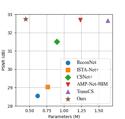
Figure 3: Relationship Between Model Parameters and Performance in PSNR. Comparison is on the BSD100 dataset at a compression ratio of 0.25

Robustness to noise: Compressive sensing systems almost always deal with some level of noise during image acquisition [1]. Therefore, it is prudent to verify the reliability of our model when the measurements are corrupted with different degrees of noise. To this end, we follow [35], by adding Gaussian noise with different standard deviations ($\sigma$) to the input before inference on the BSD100 dataset. Table 2 illustrates that our model is more robust than previous work, even-though we do not augment our images with distortions in our training pipeline. It can be noted that MOSAIC compares better as $\gamma$ increases, with larger margins. This experiment also validates the generalizability of our model, and its ability to better isolate and reconstruct the underlying image pattern, distinguishing from random noise.

Table 2: Evaluation of robustness to noise during inference on BSD100 dataset.

$\sigma$	$\gamma$	ISTA-Net+  [44]	CSNet+ [36]	AMP-Net-9BM [48]	TransCS [35]	MOSAIC (Ours)
0.001	0.04	19.50/0.4401	25.18/0.6503	24.89/0.6461	26.11/0.6790	28.22/0.8337
0.001	0.10	21.19/0.5334	27.30/0.7504	26.97/0.7480	28.19/0.7738	29.34/0.8630
0.001	0.25	22.20/0.6295	29.01/0.7847	29.26/0.8186	30.14/0.8251	34.68/0.9589
0.002	0.04	18.54/0.3993	25.15/0.6474	24.79/0.6405	25.97/0.6697	28.21/0.8336
0.002	0.10	20.02/0.4701	27.02/0.6873	26.59/0.7251	27.73/0.7461	29.34/0.8630
0.002	0.25	20.50/0.5368	27.33/0.7031	28.06/0.7604	28.79/0.7628	34.65/0.9583
0.004	0.04	17.45/0.3631	24.53/0.5984	24.59/0.6271	25.74/0.6528	28.21/0.8331
0.004	0.10	18.70/0.3890	25.03/0.6196	25.94/0.6854	26.99/0.6989	29.32/0.8620
0.004	0.25	18.73/0.4254	25.10/0.6522	26.49/0.6787	27.04/0.6789	34.54/0.9560

4.3 Qualitative Results

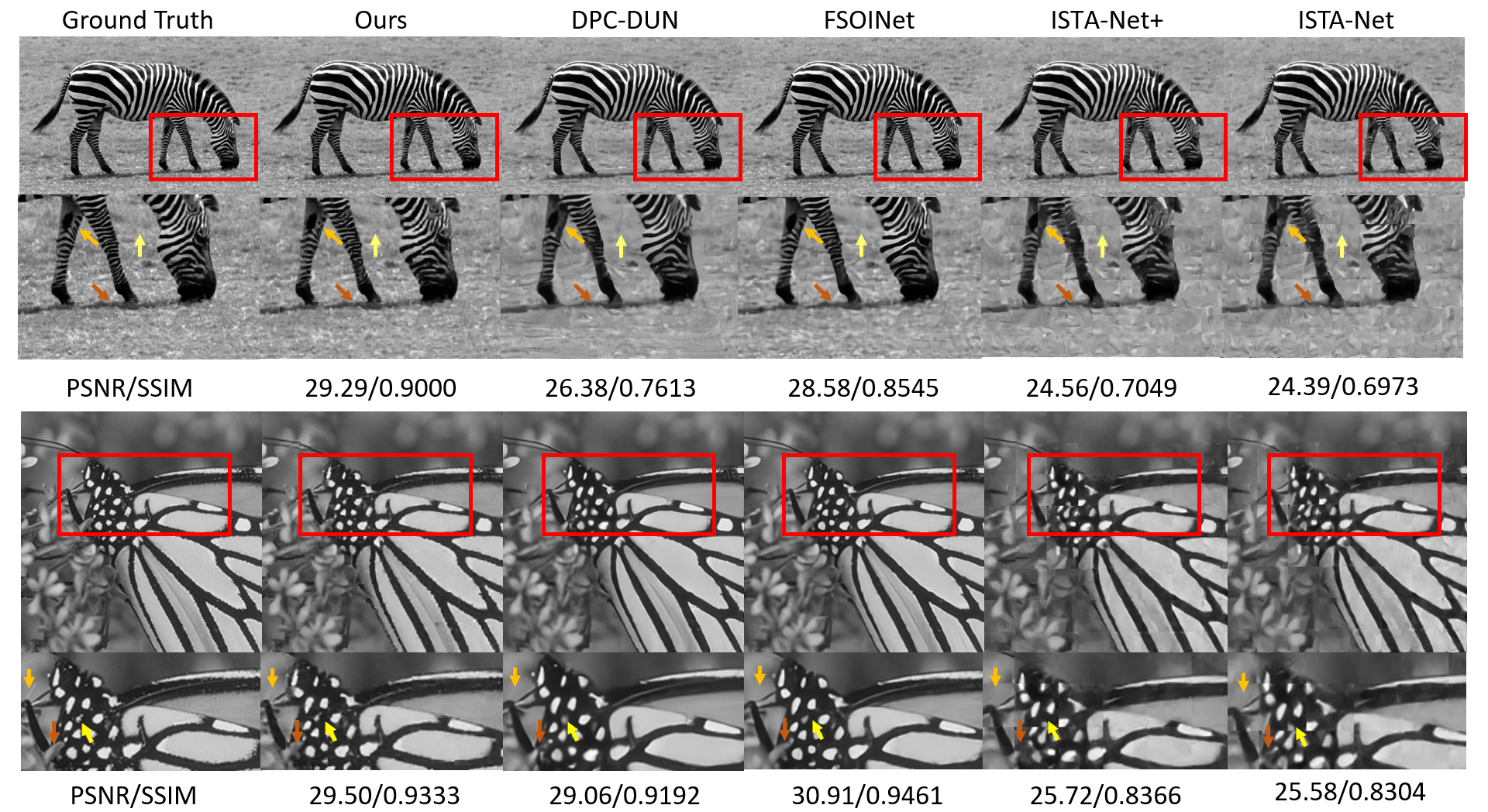
Figure 4: Performance comparison of different models at a compression ratio of 0.1 using images from the Set11 dataset.

A visual analysis of the test reconstructions are provided to further validate the quantitative results. Compared to recent deep CS reconstruction tasks, it can be observed that visual level discrepancies become obvious only at low compression ratios. As an example, the Zebra image from Set14 dataset [45] is compared in Figure 4, which shows that the detail in both the foreground and background are harder to capture.

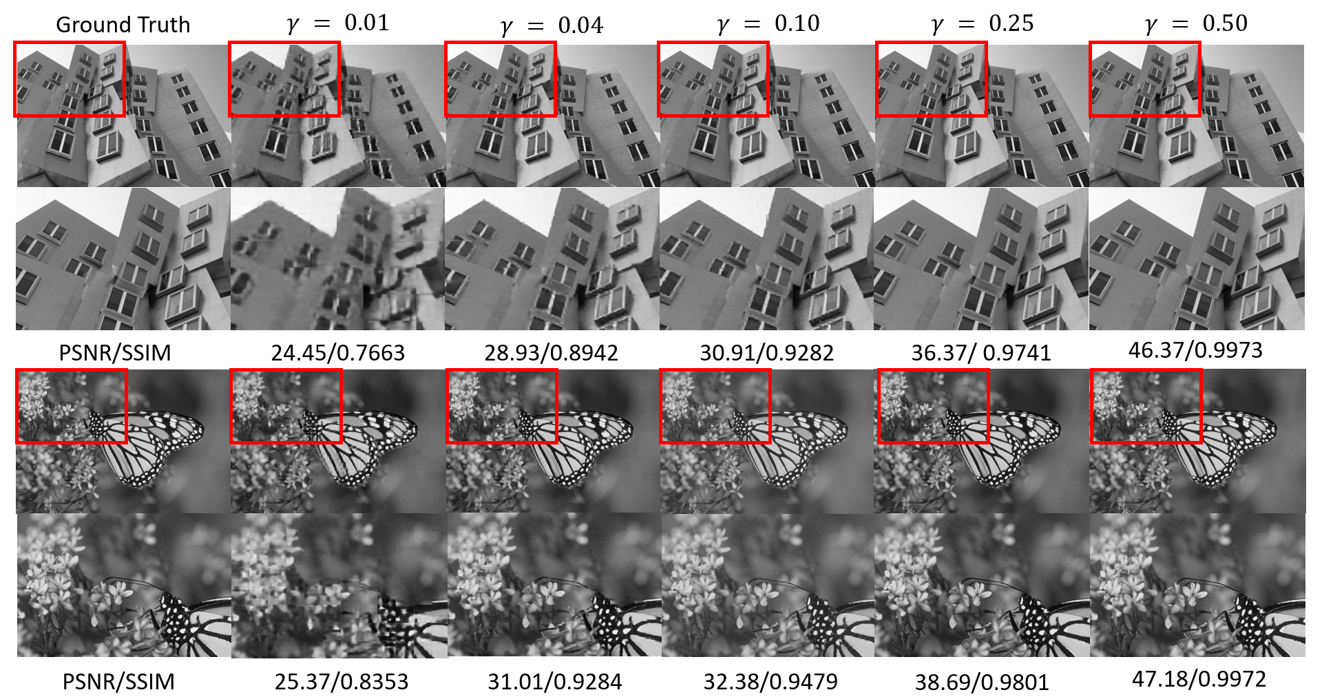
Figure 5: Visualizing the performance of our model across various compression ratios using images from the Set11 and Urban100 datasets

Since MOSAIC does not rely on convolutional layers to refine a predicted image, it is less likely to filter out high frequency content. This can be observed in the butterfly image from Set11 [23] in Figure 4, where the small white patches, and fine grained detail are lost in all previous work, while it is preserved in our reconstruction.

We have compared only across the luminance channel since it is the only channel that is compared quantitatively among related literature  [47, 44, 6].

4.4 Ablation Study

We ablate the effectiveness of different modules of MOSAIC model to identify the importance of each of them. To be easily comparable across ablations, we use $\gamma=0.25$.

Effect of transformer block count: We change the transformer block count in the encoder and decoder parts of the reconstruction module. Evaluation metrics are shown in Table 3(a). It is observed that the model output shows only a slight variation for most of the larger configurations. Therefore, we select the 16-layer configuration as our baseline model.

Table 3: Ablation results

(a) Comparing reconstruction performance with different transformer block counts on Set11 dataset at 0.25 compression ratio.

Encoder	Decoder	Parameters	PSNR/SSIM
32	32	847K	35.28/0.967
20	20	542K	33.47/0.956
16	16	440K	36.11/0.970
12	12	339K	36.71/0.976
8	8	237K	33.56/0.952
4	4	136K	33.77/0.960

(b) Comparison of reconstruction performance with and without the proposed embedding scheme $\mathbf{E}$ for 0.25 compression ratio.

Dataset	PSNR/SSIM
	No Embedding	$\mathbf{E}_{i,j}$
Set11	21.72/0.592	36.00/0.970
BSD100	23.60/0.557	34.79/0.959
Urban100	19.95/0.486	32.53/0.963

Effect of embedding $\mathbf{E}$:
We replace $\mathbf{E}_{i,j}$ of equation 4 with a matrix of all ones, to evaluate the effect of embedding the sampling matrix information ($\phi_{i},\phi_{j}$ ) into the measurement $\mathbf{y}_{i,j}$ before being input to the transformer. The ablation results on test sets are shown on Table 3(b). The performance without $\mathbf{E}_{i,j}$ dropped by 50% for PSNR, and more than 60% for SSIM. It is clear that our intuitions of decomposing a sample $\mathbf{X}$ as in equation 5 resulted in an structured embedding, which is critical for accurate reconstruction. Even-though a sufficiently parametrized deep learning model should in theory be able to learn such decompositions, the strong inductive bias given by explicitly using $\phi_{i}^{T}\phi_{j}$ has shown increase performance significantly.

5 Discussion

Interpreting results: MOSAIC is able to improve the PSNR values with increments ranging from $+2\ \text{dB}$ to $+7\ \text{dB}$, compared to previous models. Since PSNR focuses on the pixel-level differences between images, it can be inferred that our proposed method is effective in preserving fine-grained detail in the reconstruction. Additionally, our model is able to achieve better performance in SSIM, implying that it performs well in terms of perceptual aspects and preserves the structural similarity. Although SOTA for higher compression ratios was already high (around $0.98$), MOSAIC was able to push the limit even further, demonstrating the effectiveness in the proposed method.

Choice of sampling basis: The binary state of $\mathcal{H}$ is often seen as an inhibitor for CS reconstruction accuracy [35]. However we have empirically disproven this idea through our results. Other popular choices for $\Phi$ could be a wavelet basis, or a DCT basis, depending on the specific application. Future work could explore these choices, and the effect of using structure-specific embeddings in the reconstruction models.

Adaptive selection of measurement vectors: More recent work on deep learning methods for CS reconstruction attempt at selecting the sampling rows adaptively. In CASNet [6], it samples each patch at an adaptive compression rate, so as to more efficiently allocate the given number of samples $m$ for an overall compression rate. Without such sophisticated adaptive sampling, MOSAIC outperforms CASNet, which further alludes to the effectiveness of the proposed reconstruction. (Table 1, Set11 dataset [23])

Limitations and future directions; Our proposed formalisms are derived for sampling matrices which have orthogonal, and separable transforms. Therefore, the formalism and approaches for training on random sampling matrices could be explored. Furthermore, MOSAIC uses a patching approach for processing images, which creates the potential for blocking artifacts in reconstructions. Currently, there are models such as DPC-DUN [38] which use overlapping blocks, although it is harder to reproduce in practical imaging systems. Therefore, it is promising to explore methods to overcome such qualitative defects without compromising applicability.

6 Conclusion

In this work we introduce MOSAIC, a masked-encoding-based inverse solver for compressive sensing (CS). In MOSAIC we reformulate the CS inverse problem as a learnable measurement unmasking problem in a latent representation. Moreover, MOSAIC exploits the structure of a fixed sampling basis to embed measurements into a high-dimensional representation before encoding. Our results suggest that the proposed embedding, along with masked optimisation, allows efficient reconstructions. To this end, MOSAIC achieves the state of the art across a wide range of compression ratios on a variety of benchmarks, even outperforming methods with learnable sampling matrices. We believe that the strong inductive bias given by explicitly using the structure of the measurement vectors, accounts for such improvements. Thus, we demonstrate the possibility of learning a general inverse mapping from a random selection of samples, for CS reconstruction through a given basis.

7 Supplementary

7.1 More details in the experimental setup

Distributed training The base model was trained on two Nvidia Quadro RTX 6000 GPUs (24GB RAM), while ablations, and extensive experiments were run on four NVIDIA A100-SXM4-40GB GPUs (32GB RAM). The accelerate library [15] was employed to enable the codes to be trained on any distributed configuration.

Training images The proposed architecture was designed for reconstructing an image of a fixed size. For our experiments, the fixed size of an input $\mathbf{X}$ was (32,32). In order to accommodate images with other sizes and shapes, images were zero-padded and sliced to generate non-overlapping patches as a pre-processing step during validation and testing [47, 44]. The training dataset CIFAR10 [22], contained images of same size. Datasets BSD500 [26] (used for fine-tuning), and BSD100 [26], Set11 [23], Urban100 [20] contained images with different (larger) dimensions. This required the padding and patching process as pre-processing step, and the stitching of these patches together as post-processing.

Training and inference We used the functions provided by torch-metrics library with default parameters to calculate the PSNR, SSIM metrics. Validation accuracy (PSNR) curves for different compression ratios are shown in figure 6. We noticed that MOSAIC converges faster for low compression ratios. Therefore, it is possible that some models would require more training than the recommended 500 epochs with changes in training data.
We analysed existing literature, to find the most commonly inferred test datasets. Our trained model was then inferred on these datasets, and the results were reported in the main results table. Our complete analysis is shown in Table 4, where ‘-’ indicates unavailable model weights, which require separate training, and ‘*’ indicates results that have been reproduced with publicly available model weights.

7.2 Extended Quantitative Results

Random sampling In contrast to preceding approaches, we propose a reconstruction model that is applicable for any random choice of measurements. To inspect the consistency of reconstruction performance, we infer our model on multiple random samples on test data.

We reported the mean and standard deviation values of the inferences in Table 4. where the inferences are repeated for 10 random instances of the compressed sampling. The random seed was changed each instance, which created a different sampling of $\mathbf{Y}$. The low standard deviation indicates the consistency of the proposed reconstruction for any random sample.

Robustness to noise We have reported on the ability of MOSAIC to reconstruct images, even in instances the input image is corrupted with Gaussian noise. This was being consistent with previous work [35], in selecting the compression ratios ($\gamma$), and the standard deviation ($\sigma$) for the noise. Here we extend the comparison to a wider range of $\sigma$ and $\gamma$ in Table 6, to analyse the effect of higher levels of corruption in inputs for MOSAIC.

Evaluating across compression ratios
In general, a MOSAIC model trained specifically for a given compression ratio $\gamma$ outperformed other versions of the model in terms of validation and test metrics. Interestingly, similar to the empirical observations made in [28], we noticed that MOSAIC trained on compression ratios that are binary fractions, ($\gamma=0.125=1/4,\ \gamma=0.03125=1/32$) slightly outperforms models trained on other relatively closer $\gamma$. Maintaining consistency, we have not considered these results in our comparisons in Table 4, although we report this observation in Table 5.

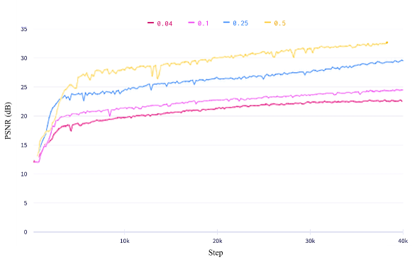
Figure 6: A model showing the validation PSNR curves for the $\gamma=0.5,0.25,0.1\text{ and }0.04$ MOSAIC models

Table 4: PSNR/SSIM metric comparisons of different models on test datasets

		PSNR/SSIM for sampling ratios
Dataset	Method	0.01	0.04	0.1	0.25	0.5
Set5	CSNet+ [36]	-	28.22/0.809	32.22/0.911	36.35/0.958	41.61/0.983
	ISTA-Net++ [44]	-	-	-	-	-
	AMP-Net [48]	-	27.71/0.811	31.79/0.898	36.68/0.953	41.52/0.979
	TransCS [35]	-	29.02/0.842	33.56/0.924	38.26/0.965	43.42/0.985
	FSOINet [7]	23.18/0.639*	28.60/0.846*	33.04/0.924*	37.53/0.963*	42.65/0.984*
	CASNet [6]	-	-	-	-	-
	DPCDUN [38]	-	-	31.12/0.893*	35.96/0.9471*	41.07/0.978*
	MOSAIC (mean)	25.95/0.697	31.15/0.899	32.80/0.920	38.34/0.969	47.21/0.996
	MOSAIC std	0.0456/0.0023	0.0738/0.0011	0.08/0.0004	0.0000/0.0426	0.2804/0.0004
Set11	CSNet+ [36]	20.67/0.541	24.83/0.784	28.34/0.858	33.34/0.939	38.47/0.979
	ISTA-Net++ [44]	18.29/0.459	22.91/0.679	27.54/0.835	32.70/0.927	37.47/0.967
	AMP-Net [48]	20.20/0.558	25.26/0.772	29.40/0.878	34.63/0.948	40.33/0.980
	TransCS [35]	-	-	-	-	-
	FSOINet [7]	21.73/0.594	26.37/0.812*	30.44/0.902	35.80/0.960*	41.08/0.983
	CASNet [6]	21.97/0.614	26.41/0.815	30.36/0.901	35.67/0.959	40.93/0.983
	DPC-DUN [38]	-	-	29.40/0.880	34.69/0.948	39.84/0.978
	MOSAIC (mean)	23.68/0.710	28.28/0.871	29.93/0.905	36.02/0.970	45.46/0.997
	MOSAIC std	0.0375/0.0007	0.0546/0.0009	0.0236/0.0003	0.036/0.0	0.2812/0.0
BSD100	CSNet+ [36]	-	25.79/0.674	28.29/0.796	31.50/0.899	36.35/0.964
	ISTA-Net++ [44]	19.98/0.449	23.26/0.587	25.86/0.717	29.48/0.854	33.97/0.941
	AMP-Net [48]	23.45/0.554	26.35/0.681	28.87/0.792	32.69/0.903	37.71/0.967
	TransCS [35]	-	26.25/0.689	28.79/0.806	32.66/0.910	37.70/0.969
	FSOINet [7]	22.76/0.528*	25.44/0.686*	28.01/0.806*	31.90/0.911*	37.02/0.970*
	CASNet [6]	-	-	-	-	-
	DPCDUN [38]	-	-	26.54/0.746*	30.43/0.874*	35.32/0.954*
	MOSAIC (mean)	24.59/0.577	28.12/0.832	29.33/0.866	34.63/0.955	45.07/0.996
	MOSAIC std	0.008/0.0	0.0068/0.0003	0.0066/0.0	0.0074/0.0	0.0319/0.0
Urban100	CSNet+ [36]	-	21.17/0.611	24.01/0.783	27.68/0.897	33.32/0.966
	ISTA-Net++[44]	17.48/0.416	20.96/0.599	24.66/0.762	29.51/0.894	34.41/0.957
	AMP-Net [48]	20.90/0.533	24.15/0.703	27.38/0.827	32.19/0.926	37.51/0.973
	TransCS [35]	-	23.23/0.702	26.73/0.842	31.72/0.933	37.20/0.976
	FSOINet [7]	19.87/0.522	22.71/0.704*	27.53/0.863	32.17/0.950*	37.80/0.978
	CASNet [6]	-	-	-	-	-
	DPC-DUN [38]	-	-	26.99/0.835	32.36/0.932	37.52/0.974
	MOSAIC (mean)	21.35/0.571	25.20/0.830	26.72/0.875	32.43/0.961	42.41/0.996
	MOSAIC std	0.0057/0.0003	0.0058/0.0005	0.0048/0.0003	0.0079/0.0	0.0741/0.0

Table 5: MOSAIC trained on $\gamma=0.125$, and inferred on samples of $\gamma=0.1$

Dataset	PSNR/SSIM
	MOSAIC (0.1)	MOSAIC (0.125)	Recent best
Set11	27.93/0.905	30.43/0.905	30.44 (FSOINet)/0.902 (FSOINet)
BSD100	29.33/0.886	29.93/0.884	28.87 (AmpNet)/0.806 (TransCS)
Urban100	26.72/0.875	27.53/0.891	27.53 (FSOINet)/0.863 (FSOINet)

Table 6: Evaluation of robustness to noise during inference on BSD100 dataset.

$\sigma$	PSNR for sampling ratios and reduction in accuracy compared to $\sigma=0$
	0.01	0.04	0.1	0.25	0.5
0.001	24.58 ($\downarrow 0.01$)	28.11 ($\downarrow 0.01$)	29.32 ($\downarrow 0.01$)	34.63 ($\downarrow 0.00$)	44.88 ($\downarrow 0.19$)
0.002	24.58 ($\downarrow 0.01$)	28.11 ($\downarrow 0.01$)	29.32 ($\downarrow 0.01$)	34.60 ($\downarrow 0.03$)	44.43 ($\downarrow 0.64$)
0.004	24.58 ($\downarrow 0.01$)	28.10 ($\downarrow 0.02$)	29.30 ($\downarrow 0.03$)	34.48 ($\downarrow 0.15$)	43.06 ($\downarrow 2.01$)
0.01	24.57 ($\downarrow 0.02$)	28.04 ($\downarrow 0.08$)	29.19 ($\downarrow 0.14$)	33.76 ($\downarrow 0.87$)	38.69 ($\downarrow 6.38$)
0.02	24.55 ($\downarrow 0.04$)	27.83 ($\downarrow 0.29$)	28.79 ($\downarrow 0.54$)	31.90 ($\downarrow 1.73$)	33.63 ($\downarrow 11.44$)
0.04	24.46 ($\downarrow 0.13$)	27.02 ($\downarrow 1.1$)	27.47 ($\downarrow 1.86$)	28.15 ($\downarrow 6.48$)	27.89 ($\downarrow 17.18$)
0.1	23.79 ($\downarrow 0.80$)	23.38 ($\downarrow 4.74$)	22.95 ($\downarrow 6.38$)	21.23 ($\downarrow 13.40$)	20.06 ($\downarrow 27.01$)
0.2	21.77 ($\downarrow 2.82$)	18.79 ($\downarrow 9.33$)	17.92 ($\downarrow 11.41$)	15.58 ($\downarrow 19.05$)	14.28 ($\downarrow 30.79$)
0.4	17.92 ($\downarrow 6.67$)	13.87 ($\downarrow 14.25$)	12.15 ($\downarrow 17.18$)	10.34 ($\downarrow 24.29$)	8.88 ($\downarrow 36.19$)

Table 7: Evaluation of robustness to noise during inference on BSD100 dataset.

$\sigma$	SSIM for sampling ratios and reduction in accuracy compared to $\sigma=0$
	0.01	0.04	0.1	0.25	0.5
0.001	0.577 ($\downarrow 0.000$)	0.832 ($\downarrow 0.000$)	0.866 ($\downarrow 0.000$)	0.955 ($\downarrow 0.000$)	0.994 ($\downarrow 0.002$)
0.002	0.577 ($\downarrow 0.000$)	0.832 ($\downarrow 0.000$)	0.866 ($\downarrow 0.000$)	0.954 ($\downarrow 0.001$)	0.993 ($\downarrow 0.003$)
0.004	0.577 ($\downarrow 0.000$)	0.832 ($\downarrow 0.000$)	0.865 ($\downarrow 0.001$)	0.951 ($\downarrow 0.004$)	0.988 ($\downarrow 0.008$)
0.01	0.576 ($\downarrow 0.001$)	0.828 ($\downarrow 0.004$)	0.858 ($\downarrow 0.008$)	0.933 ($\downarrow 0.022$)	0.956 ($\downarrow 0.040$)
0.02	0.575 ($\downarrow 0.002$)	0.814 ($\downarrow 0.018$)	0.833 ($\downarrow 0.033$)	0.876 ($\downarrow 0.079$)	0.874 ($\downarrow 0.122$)
0.04	0.569 ($\downarrow 0.008$)	0.761 ($\downarrow 0.071$)	0.754 ($\downarrow 0.112$)	0.734 ($\downarrow 0.221$)	0.707 ($\downarrow 0.289$)
0.1	0.531 ($\downarrow 0.046$)	0.552 ($\downarrow 0.280$)	0.527 ($\downarrow 0.339$)	0.451 ($\downarrow 0.504$)	0.411 ($\downarrow 0.585$)
0.2	0.433 ($\downarrow 0.144$)	0.352 ($\downarrow 0.480$)	0.328 ($\downarrow 0.538$)	0.242 ($\downarrow 0.713$)	0.219 ($\downarrow 0.777$)
0.4	0.279 ($\downarrow 0.298$)	0.184 ($\downarrow 0.648$)	0.199 ($\downarrow 0.667$)	0.110 ($\downarrow 0.845$)	0.108 ($\downarrow 0.888$)

7.3 Extended Qualitative Results

Comparison with other models We have reported the compression ratio $\gamma=0.1$ qualitative comparison in the main paper. This is since the differences among models are visually apparent at such low compression ratios. For higher $\gamma=0.25,\ 0.5$, although there are differences in the PSNR/SSIM metrics, these differences are not prominent in the visualisation. This is evident from the comparison in Figures 8,9 For lower compression ratios, we use $\gamma=0.1$ (Figure 7) since it has the lowest compression ratio with common published weights among related work. We observe better sharpness and reconstruction of fine details in our method. Additionally, we include a comparison of 3-channel images (Figure 10), following related work[44, 48, 38] in which only the Lumina(Y) channel is processed through the CS algorithm. Please zoom in for a clear comparison.

Visualising reconstructions of corrupted inputs
We further evaluate the robustness to noise of MOSAIC, compared to recent work, in a qualitative sense for a higher noise $\sigma=\ 0.1$, and compression ratios $\gamma=0.1,\ 0.25$ in Figure 11. This demonstrates that although MOSAIC is resilient to low noise levels, it is less robust in higher $\sigma$. Although our main goal is not to achieve noise robustness, future work could explore on how to improve noise-robustness through incorporating the MOSAIC architecture with noise statistics .

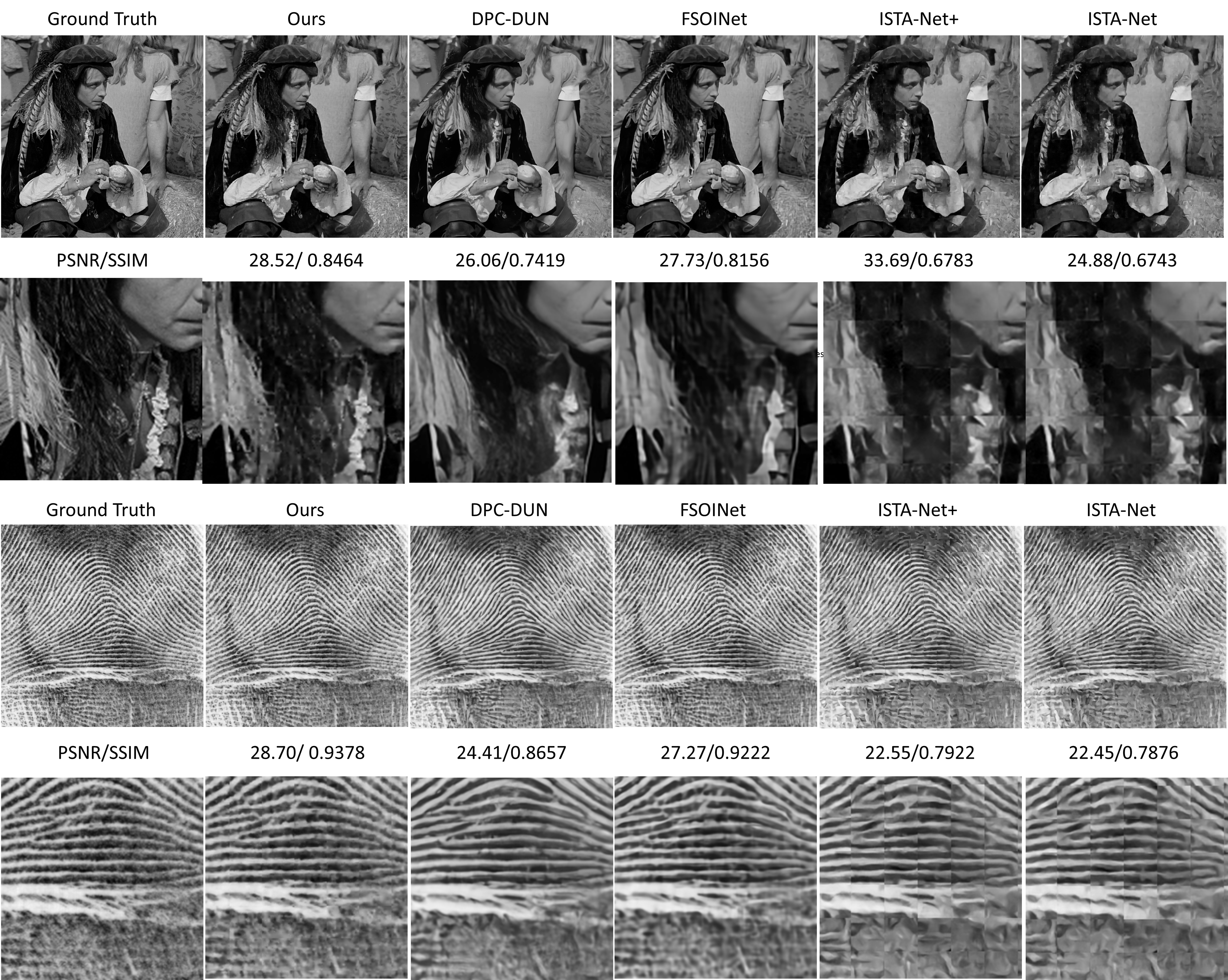
Figure 7: Comparing MOSAIC to other models, showing comparable visual differences for $\gamma=0.1$. Ground-truth images are from Set14 and Set11 datasets respectively.

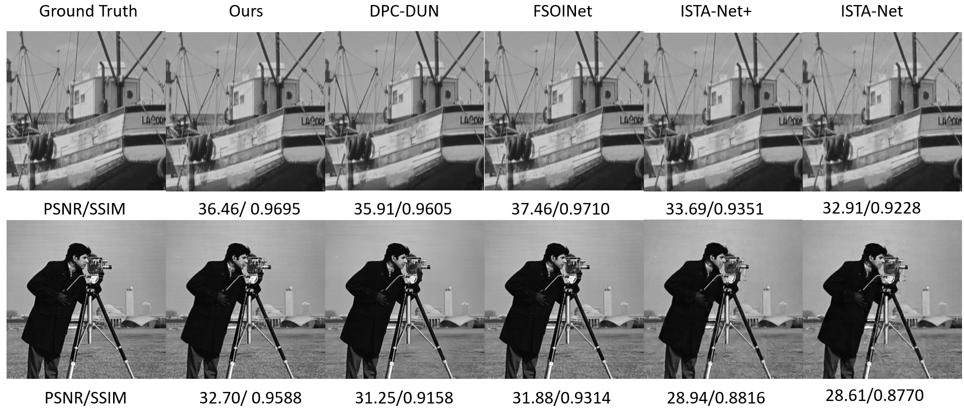
Figure 8: Comparing MOSAIC to other models, showing the almost negligeble visual differences for $\gamma=0.25$. Ground-truth images are from the Set11 dataset.

Figure 9: Comparing MOSAIC to other models, showing the almost negligeble visual differences for $\gamma=\ 0.5$. Ground-truth images are from the Set11 dataset.

Figure 10: Comparing MOSAIC to other models,depicting visual differences for $\gamma=\ 0.1$ in a 3-channel visualisation. Ground-truth images are taken from Set5 and Set14 datasets respectively.

Figure 11: Qualitative evaluation of reconstruction models for a Gaussian-noise corrupted image at $\sigma=0.1$.

7.4 Extended Ablations

Choice of sampling matrix
The Walsh-Hadamard matrix $\mathbf{\Phi}=\mathcal{H}_{(1,-1)}$ which was used in MOSAIC has binary elements, with {1, -1} entries. This choice was motivated by it’s orthogonal property, and empirical evidence of better learning (Table 8); when compared to the non-orthogonal Hadamard matrix $\mathcal{H}_{(1,0)}$ with {1, 0} elements. Considering a practical implementation with a sampling scheme employing $\mathcal{H}_{(1,0)}$, we note the relation between the sampled measurements from the ith row of both matrices. Specifically, $p_{i}=\mathcal{H}_{(1,0),\ i}\ \mathbf{x}$ is related to the measurement $q_{i}=\mathcal{H}_{(1,-1),\ i}\ \mathbf{x}$, through a measurement $\mathbf{1}^{T}\mathbf{x}$ as follows.

$$p_{i} =(q_{i}+\mathbf{1}^{T}\mathbf{x})/2$$

Hence, provided that the first row of $\mathcal{H}_{(1,0)}$ (which is $\mathbf{1}^{T}$), is always selected as a measurement vector, one could use the above equation to create a mapping between MOSAIC’s proposed reconstruction algorithm, and a more practically feasible CS scheme. Noting that the above relation would not hold exactly under noisy measurements, one should consider analysing the noise distributions in measurement space.

Parameter counts
Following recent work, we compare the parameter count of MOSAIC with other models at different compression ratios in figure 12. The values for other models are reported from previous work [35], and publicly available inference codes.

Table 8: Comparison of $\mathcal{H}_{(1,0)}$ with $\mathcal{H}_{(1,-1)}$
at $\gamma=0.25$

$\mathbf{\Phi}$	val. PSNR	val. SSIM
$\mathcal{H}_{(1,0)}$	12.4	0.14
$\mathcal{H}_{(1,-1)}$	33.0	0.96

Figure 12: Comparison of PSNR with the number of parameters: for $\gamma=0.1\text{ and }\gamma=0.25$

References

- [1] Ery Arias-Castro and Yonina C. Eldar. Noise folding in compressed sensing. IEEE Signal Processing Letters, 18(8):478–481, 2011.
- [2] Hangbo Bao, Li Dong, Songhao Piao, and Furu Wei. BEit: BERT pre-training of image transformers. In International Conference on Learning Representations, 2022.
- [3] Thomas Blumensath and Mike E. Davies. Iterative hard thresholding for compressed sensing. Applied and Computational Harmonic Analysis, 27(3):265–274, 2009.
- [4] Jian-Feng Cai, Emmanuel J Candès, and Zuowei Shen. Iterative thresholding for sparse approximations. Communications on Pure and Applied Mathematics, 60(6):661–674, 2007.
- [5] E.J. Candes, J. Romberg, and T. Tao. Robust uncertainty principles: exact signal reconstruction from highly incomplete frequency information. IEEE Transactions on Information Theory, 52(2):489–509, 2006.
- [6] Bin Chen and Jian Zhang. Content-aware scalable deep compressed sensing. IEEE Transactions on Image Processing, 31:5412–5426, 2022.
- [7] Wenjun Chen, Chunling Yang, and Xin Yang. Fsoinet: feature-space optimization-inspired network for image compressive sensing. In ICASSP 2022-2022 IEEE International Conference on Acoustics, Speech and Signal Processing (ICASSP), pages 2460–2464. IEEE, 2022.
- [8] Ingrid Daubechies, Michel Defrise, and Christine De Mol. An iterative thresholding algorithm for linear inverse problems with a sparsity constraint. Communications on Pure and Applied Mathematics: A Journal Issued by the Courant Institute of Mathematical Sciences, 57(11):1413–1457, 2004.
- [9] Jacob Devlin, Ming-Wei Chang, Kenton Lee, and Kristina Toutanova. Bert: Pre-training of deep bidirectional transformers for language understanding. arXiv preprint arXiv:1810.04805, 2018.
- [10] David L Donoho, Arian Maleki, and Andrea Montanari. Approximate message passing for sparse linear systems. Proceedings of the National Academy of Sciences, 107(5):1970–1976, 2010.
- [11] D.L. Donoho. Compressed sensing. IEEE Transactions on Information Theory, 52(4):1289–1306, 2006.
- [12] Alexey Dosovitskiy, Lucas Beyer, Alexander Kolesnikov, Dirk Weissenborn, Xiaohua Zhai, Thomas Unterthiner, Mostafa Dehghani, Matthias Minderer, Georg Heigold, Sylvain Gelly, Jakob Uszkoreit, and Neil Houlsby. An image is worth 16x16 words: Transformers for image recognition at scale. In International Conference on Learning Representations, 2021.
- [13] Adam Dziedzic, John Paparrizos, Sanjay Krishnan, Aaron Elmore, and Michael Franklin. Band-limited training and inference for convolutional neural networks. In International Conference on Machine Learning, pages 1745–1754. PMLR, 2019.
- [14] Michael Elad and Michal Aharon. Image denoising via sparse and redundant representations over learned dictionaries. IEEE Transactions on Image processing, 15(12):3736–3745, 2006.
- [15] Hugging Face. Accelerate: Gpu and tpu backend for pytorch. https://huggingface.co/docs/accelerate/index, 2023.
- [16] Christoph Feichtenhofer, haoqi fan, Yanghao Li, and Kaiming He. Masked autoencoders as spatiotemporal learners. In S. Koyejo, S. Mohamed, A. Agarwal, D. Belgrave, K. Cho, and A. Oh, editors, Advances in Neural Information Processing Systems, volume 35, pages 35946–35958. Curran Associates, Inc., 2022.
- [17] Wilson Geisler. Visual perception and the statistical properties of natural scenes. Annual review of psychology, 59:167–92, 02 2008.
- [18] Kaiming He, Xinlei Chen, Saining Xie, Yanghao Li, Piotr Dollár, and Ross Girshick. Masked autoencoders are scalable vision learners. In Proceedings of the IEEE/CVF Conference on Computer Vision and Pattern Recognition, pages 16000–16009, 2022.
- [19] Geoffrey E Hinton and Ruslan R Salakhutdinov. Reducing the dimensionality of data with neural networks. science, 313(5786):504–507, 2006.
- [20] Jia-Bin Huang, Abhishek Singh, and Narendra Ahuja. Single image super-resolution from transformed self-exemplars. In Proceedings of the IEEE Conference on Computer Vision and Pattern Recognition, pages 5197–5206, 2015.
- [21] Diederik P Kingma and Jimmy Ba. Adam: A method for stochastic optimization. arXiv preprint arXiv:1412.6980, 2014.
- [22] Alex Krizhevsky. Learning multiple layers of features from tiny images. Technical report, University of Toronto, Department of Computer Science, 2009.
- [23] Kuldeep Kulkarni, Suhas Lohit, Pavan Turaga, Ronan Kerviche, and Amit Ashok. Reconnet: Non-iterative reconstruction of images from compressively sensed measurements. In Proceedings of the IEEE conference on computer vision and pattern recognition, pages 449–458, 2016.
- [24] Xinyu Li, Yanyi Zhang, Jianbo Yuan, Hanlin Lu, and Yibo Zhu. Discrete cosin transformer: Image modeling from frequency domain. In Proceedings of the IEEE/CVF Winter Conference on Applications of Computer Vision, pages 5468–5478, 2023.
- [25] Ze Liu, Yutong Lin, Yue Cao, Han Hu, Yixuan Wei, Zheng Zhang, Stephen Lin, and Baining Guo. Swin transformer: Hierarchical vision transformer using shifted windows. In Proceedings of the IEEE/CVF International Conference on Computer Vision (ICCV), 2021.
- [26] D. Martin, C. Fowlkes, D. Tal, and J. Malik. A database of human segmented natural images and its application to evaluating segmentation algorithms and measuring ecological statistics. In Proceedings Eighth IEEE International Conference on Computer Vision. ICCV 2001, volume 2, pages 416–423 vol.2, 2001.
- [27] Christopher A. Metzler, Ali Mousavi, and Richard G. Baraniuk. Learned D-AMP: Principled neural network based compressive image recovery. In Isabelle Guyon, Ulrike von Luxburg, Samy Bengio, Hanna M. Wallach, Rob Fergus, S. V. N. Vishwanathan, and Roman Garnett, editors, NIPS, pages 1772–1783, 2017.
- [28] Ben Mildenhall, Pratul P Srinivasan, Matthew Tancik, Jonathan T Barron, Ravi Ramamoorthi, and Ren Ng. Nerf: Representing scenes as neural radiance fields for view synthesis. Communications of the ACM, 65(1):99–106, 2021.
- [29] A Oppenheim, Jae Lim, Gary Kopec, and SC Pohlig. Phase in speech and pictures. In ICASSP’79. IEEE International Conference on Acoustics, Speech, and Signal Processing, volume 4, pages 632–637. IEEE, 1979.
- [30] Alan V Oppenheim and Jae S Lim. The importance of phase in signals. Proceedings of the IEEE, 69(5):529–541, 1981.
- [31] Zhijin Qin, Jiancun Fan, Yuanwei Liu, Yue Gao, and Geoffrey Ye Li. Sparse representation for wireless communications: A compressive sensing approach. IEEE Signal Processing Magazine, 35(3):40–58, 2018.
- [32] Nasim Rahaman, Aristide Baratin, Devansh Arpit, Felix Draxler, Min Lin, Fred Hamprecht, Yoshua Bengio, and Aaron Courville. On the spectral bias of neural networks. In Kamalika Chaudhuri and Ruslan Salakhutdinov, editors, Proceedings of the 36th International Conference on Machine Learning, volume 97 of Proceedings of Machine Learning Research, pages 5301–5310. PMLR, 09–15 Jun 2019.
- [33] Meenu Rani, S. B. Dhok, and R. B. Deshmukh. A systematic review of compressive sensing: Concepts, implementations and applications. IEEE Access, 6:4875–4894, 2018.
- [34] Yongming Rao, Wenliang Zhao, Zheng Zhu, Jiwen Lu, and Jie Zhou. Global filter networks for image classification. Advances in neural information processing systems, 34:980–993, 2021.
- [35] Minghe Shen, Hongping Gan, Chao Ning, Yi Hua, and Tao Zhang. Transcs: A transformer-based hybrid architecture for image compressed sensing. IEEE Transactions on Image Processing, 31:6991–7005, 2022.
- [36] Wuzhen Shi, Feng Jiang, Shaohui Liu, and Debin Zhao. Image compressed sensing using convolutional neural network. IEEE Transactions on Image Processing, 29:375–388, 2019.
- [37] Wuzhen Shi, Feng Jiang, Shaohui Liu, and Debin Zhao. Scalable convolutional neural network for image compressed sensing. In Proceedings of the IEEE/CVF Conference on Computer Vision and Pattern Recognition, pages 12290–12299, 2019.
- [38] Jiechong Song, Bin Chen, and Jian Zhang. Dynamic path-controllable deep unfolding network for compressive sensing. IEEE Transactions on Image Processing, 2023.
- [39] A. van der Schaaf and J.H. van Hateren. Modelling the power spectra of natural images: Statistics and information. Vision Research, 36(17):2759–2770, 1996.
- [40] Pascal Vincent, Hugo Larochelle, Isabelle Lajoie, Yoshua Bengio, and Pierre-Antoine Manzagol. Stacked denoising autoencoders: Learning useful representations in a deep network with a local denoising criterion. Journal of Machine Learning Research, 11(110):3371–3408, 2010.
- [41] Jiahao Xie, Wei Li, Xiaohang Zhan, Ziwei Liu, Yew Soon Ong, and Chen Change Loy. Masked frequency modeling for self-supervised visual pre-training. In Proceedings of the IEEE/International Conference on Learning Representations, 2023.
- [42] Zhenda Xie, Zheng Zhang, Yue Cao, Yutong Lin, Jianmin Bao, Zhuliang Yao, Qi Dai, and Han Hu. Simmim: A simple framework for masked image modeling. In International Conference on Computer Vision and Pattern Recognition (CVPR), 2022.
- [43] Y. Yang, J. Sun, H. Li, and Z. Xu. Admm-csnet: A deep learning approach for image compressive sensing. IEEE Transactions on Pattern Analysis and Machine Intelligence, 42(03):521–538, mar 2020.
- [44] Di You, Jingfen Xie, and Jian Zhang. Ista-net++: Flexible deep unfolding network for compressive sensing. In 2021 IEEE International Conference on Multimedia and Expo (ICME), pages 1–6, 2021.
- [45] Roman Zeyde, Michael Elad, and Matan Protter. On single image scale-up using sparse-representations. Conference on Curves and Surfaces, 2010. Available at: https://people.csail.mit.edu/torralba/shortCourseRLOC/lectures/lectureSparseRepresentations.pdf.
- [46] Haotian Zhang, Pengchuan Zhang, Xiaowei Hu, Yen-Chun Chen, Liunian Li, Xiyang Dai, Lijuan Wang, Lu Yuan, Jenq-Neng Hwang, and Jianfeng Gao. Glipv2: Unifying localization and vision-language understanding. In S. Koyejo, S. Mohamed, A. Agarwal, D. Belgrave, K. Cho, and A. Oh, editors, Advances in Neural Information Processing Systems, volume 35, pages 36067–36080. Curran Associates, Inc., 2022.
- [47] J. Zhang and B. Ghanem. ISTA-Net: Interpretable optimization-inspired deep network for image compressive sensing. In 2018 IEEE/CVF Conference on Computer Vision and Pattern Recognition (CVPR), pages 1828–1837, Los Alamitos, CA, USA, jun 2018. IEEE Computer Society.
- [48] Zhonghao Zhang, Yipeng Liu, Jiani Liu, Fei Wen, and Ce Zhu. Amp-net: Denoising-based deep unfolding for compressive image sensing. IEEE Transactions on Image Processing, 30:1487–1500, 2020.