Gauss–Southwell type descent methods for
low-rank matrix optimization

Abstract

We consider gradient-related methods for low-rank matrix optimization with a smooth cost function. The methods operate on single factors of the low-rank factorization and share aspects of both alternating and Riemannian optimization. Two possible choices for the search directions based on Gauss–Southwell type selection rules are compared: one using the gradient of a factorized non-convex formulation, the other using the Riemannian gradient. While both methods provide gradient convergence guarantees that are similar to the unconstrained case, numerical experiments on a quadratic cost function indicate that the version based on the Riemannian gradient is significantly more robust with respect to small singular values and the condition number of the cost function. As a side result of our approach, we also obtain new convergence results for the alternating least squares method.

1 Introduction

We consider a differentiable function $f\colon{\mathbb{R}}^{m\times n}\to{\mathbb{R}}$ and the optimization problem

$$\min_{X\in{\mathbb{R}}^{m\times n}}f(X)\quad\text{s.t.}\quad\operatorname{rank}(X)\leq k,$$ (1.1)

where $m$, $n$, and $k$ are positive integers such that $k<\min\{m,n\}$. The constraint set

$$\mathcal{M}_{\leq k}=\{X\in{\mathbb{R}}^{m\times n}\colon\operatorname{rank}(X)\leq k\}$$ (1.2)

is non-convex, which makes it difficult to find the global minimum even if the function $f$ would be convex. At the same time, very efficient first-order algorithms for finding critical points can be implemented based on alternating minimization.

At the core, these algorithms are derived from the fact that the rank constraint in (1.1) can be eliminated using the bilinear factorization

$$X=LR^{\top},\quad L\in{\mathbb{R}}^{m\times k},\ R\in{\mathbb{R}}^{n\times k}$$

of a matrix of rank at most $k$. The problem (1.1) is hence equivalent to the unconstrained minimization problem

$$\min_{\begin{subarray}{c}L\in{\mathbb{R}}^{m\times k}\\ R\in{\mathbb{R}}^{n\times k}\end{subarray}}g(L,R)\qquad\text{with}\qquad g(L,R)\coloneqq f(LR^{\top}).$$ (1.3)

In the terminology of the recent work [5], the map ${\mathbb{R}}^{m\times k}\times{\mathbb{R}}^{n\times k}\to{\mathbb{R}}^{m\times n}:(L,R)\mapsto LR^{\top}$ is a smooth lift of the determinantal variety $\mathcal{M}_{\leq k}$ [3, Lecture 9] and $g$ is the lifted cost function. The class of alternating optimization methods then consists of algorithms of the following general form:

1. Given $X_{\ell}=L_{\ell}R_{\ell}^{\top}$ in factorized form, choose whether to update the $L$- or $R$-factor.

2. Depending on the choice in (1) find an update $L_{\ell+1}$ or $R_{\ell+1}$ and set $X_{\ell+1}=L_{\ell+1}R_{\ell}^{\top}$ or $X_{\ell+1}=L_{\ell}R_{\ell+1}^{\top}$, respectively.

3. Change the representation: $X_{\ell+1}=\hat{L}_{\ell+1}\hat{R}_{\ell+1}$.

In this paper we consider two different methods of this type (Algorithms 1 and 2 below), where the search directions in step (2) are gradient-related in a suitable sense and step (1) is based on a Gauss–Southwell type selection rule.

The most obvious search directions are the negative partial gradients $-\nabla_{L}\,g(L_{\ell},R_{\ell})$ and $-\nabla_{R}\,g(L_{\ell},R_{\ell})$. Unfortunately, this straightforward choice suffers from the non-uniqueness of the representation $X=LR^{\top}$ in a twofold way. First, the resulting search direction in the image space ${\mathbb{R}}^{m\times n}$ depends on the particular chosen6 representation $X_{\ell}=L_{\ell}R_{\ell}^{\top}$ (see the formulas (3.5) below), which is conceptually unsatisfying. Second, the Lipschitz constant for the partial gradients depends on the chosen representation as well, which in theory may pose nonuniform step-size restrictions for ensuring convergence. And indeed, it can be observed in practice that this has a large influence on the convergence speed. Both problems, however, can be overcome by using a so-called balanced factorization in step (3) of the above pseudocode for removing the non-uniqueness (see section 3.1), as has been proposed in several works; see, for example, [24, 25, 7, 8] where balancing is promoted via regularization.

Regarding the choice of the factor to be updated in step (1), the cyclic Gauss–Seidel type update rule is the most common choice and optimizes $L$ and $R$ alternatingly. For example, variants of the alternating gradient descent method (using the partial gradients of $g$) have been proposed and analyzed for low-rank matrix completion in [20] and [22]. However, instead of a cyclic rule, in this work we advocate for using Gauss–Southwell type update rules in which the block variable with the largest partial gradient is selected for the next update. This selection rule originates from classic iterative solvers for linear systems [18], but has also been well known for both convex and non-convex optimization ever since, see, e.g., [9, 11, 13, 15]. It ensures that the block gradient satisfies an angle condition with the full gradient of $g$. This allows for very simple convergence rate estimates for obtaining $\varepsilon$-stationary points which are almost parallel to those in the unconstrained situation. One known issue, however, also observed for other update rules, remains: the convergence rate in terms of function values or distances to solutions severely deteriorates for ill-conditioned solutions (accumulation points with a large ratio of the largest and $k$th largest singular value), one intrinsic reason being that the gradient of the function $g$ is not a robust measure for criticality on the manifold of rank-$k$ matrices.

As an alternative to the partial gradients of $g$, we will therefore also consider a different way for obtaining search directions which is motivated from a Riemannian optimization perspective. The bilinear nature of the parametrization of the set $\mathcal{M}_{\leq k}$ entails that in the smooth points $X$ of that set (the matrices of rank exactly $k$), the tangent space is decomposed into two overlapping linear spaces $T_{1}(X)+T_{2}(X)$, each of which contains $X$ and is itself entirely contained in $\mathcal{M}_{\leq k}$. It is therefore natural to use the projections of the negative gradient $-\nabla f(X_{\ell})$ onto $T_{1}(X_{\ell})$ or $T_{2}(X_{\ell})$ as search directions. These search directions are independent of the chosen factorization $X_{\ell}=L_{\ell}R_{\ell}$ but it turns out that they are actually equal to partial gradients of $g$ when the factor not to be updated is chosen to have orthonormal columns, which can be achieved by changing the representation using QR factorization after every update. Such a variant of alternating optimization with the QR factorization is usually implemented anyway for reasons of numerical stability. Interestingly, the resulting search directions are mathematically equivalent to scaled variants of partial gradients, as considered for example in [12, 22, 23], see eq. (3.12) below. Notably, in [12, §4] they are obtained from a suitable quotient geometry for the manifold of fixed-rank matrices. Corresponding methods based on cyclic or simultaneous update rules are called scaled alternating steepest descent [22] or scaled gradient descent [23]. In these works, the accelerating effect and/or robustness with respect to small singular values is clearly confirmed, see also [10, Remark 7]. As we show in the present paper, when combined with a Gauss–Southwell rule, the Riemannian derivation of these search directions as tangential projections makes it possible to analyze the convergence of the corresponding method (presented in Algorithm 2) as a gradient-related Riemannian descent method. In fact, the search directions then satisfy an angle condition with the negative Riemannian gradient (here: the projection of $-\nabla f(X_{\ell})$ onto the tangent space) and hence the convergence rate to an $\varepsilon$-Riemannian stationary point can be estimated in a simple way based on standard results. This is carried out in section 3.2. Note that a method of this type has already been proposed as a retraction-free Riemannian method in [19, Algorithm 4]. In terms of the above references, Algorithm 2 may be equivalently interpreted as a Gauss–Southwell variant of scaled gradient descent.

Having two possible choices of gradient-related search directions, it is then natural to ask which of the two is better. In terms of the rates, it turns out that the Riemannian version needs the same (estimated) number of steps for making the Riemannian gradient of $f$ smaller than $\varepsilon$ as the balanced factorized version needs for making the gradient of $g$ smaller than $\varepsilon$. However, as we show in section 3.3 the first condition implies the second (up to a small constant) but not the other way around. In this sense, we will confirm as one of the main messages of the paper that the Riemannian search directions are much more powerful than expected. Our numerical experiments in section 4 indeed confirm that it converges faster and exhibits stability with respect to small singular values of $X$, which is completely in line with aforementioned results on scaled gradient descent in [23].

One important thing to note about both of our methods is that limiting points can fail to be stationary points of the original problem (1.1), despite the Riemannian gradients converging to zero during the iteration. Although it is rarely observed in practice, such a behaviour, termed an “apocalypse” in [6], can occur when a rank drop happens at the limit; cf. Remark 3.3 below. For the Riemannian version of our algorithm, it has been recently proposed how to exclude such undesirable points as accumulation points of the algorithms by disregarding the $k$th singular value if it is below a prescribed threshold [16, Algorithm 3], while preserving the convergence rates for the Riemannian gradient as stated in our Corollary 3.5. In our work, we will largely ignore this subtlety (and assume full rank $k$ at accumulation points) in order to keep things conceptually simple.

There are two other sets of results in this work. In section 3.4, we address the fact that the algebraic convergence rates for gradients obtained from a standard analysis based on Lipschitz continuity of the gradients are usually overly pessimistic. Indeed, in practice one observes a linear convergence rate. For the Riemannian version of our Gauss–Southwell approach we provide such a result in section 3.4 provided one of the accumulation points has a positive-definite Riemannian Hessian. This proof is similar to the linear convergence proof for the Riemannian gradient method in [2, Theorem 4.5.6]. In section 3.5 we show how our arguments can be adapted for obtaining seemingly novel convergence estimates for the popular alternating least squares (ALS) algorithm. In fact, for two blocks as in low-rank matrix optimization, the cyclic rule of ALS coincides with a Gauss–Southwell rule, since one of the partial gradients is always zero by construction.

The work is structured as follows. In section 2 we review basic facts on the gradient method for $\lambda$-smooth functions on affine subspaces, which will serve as the main tool. Section 3 is the core section of this work. Section 3.1 develops the algorithm based on partial gradients of the function $g$ and balancing (Algorithm 1). The main results on gradient convergence for various step-size rules are Theorem 3.1 and Corollary 3.2. In section 3.2, the algorithm based on the decomposition of the Riemannian gradient (Algorithm 2) is developed in an analogous fashion. Main results are Theorem 3.4 and Corollary 3.5. In section 3.3 both approaches are compared; corresponding numerical experiments are presented in section 4. The results on linear convergence and ALS are in sections 3.4 and 3.5, respectively.

2 Recap of gradient descent methods

Let us first briefly recall some main results on the convergence of the gradient method for $\lambda$-smooth functions. While the results are very well known (see, e.g., [14]), we present them here for the case of a differentiable function $\phi\colon T\to{\mathbb{R}}$ defined on an affine subspace $T$ of a Euclidean vector space. In our applications later, $\phi$ will be the restriction of the cost functions $f$ and $g$, respectively, to certain subspaces. Given $x\in T$, one step of the gradient method in the space $T$ takes the form

$$x_{+}=x-h\nabla\phi(x).$$ (2.1)

Here $h>0$ is a step size that can be chosen either fixed or adaptively at each iteration. The ultimate goal of the iteration is to find a point $x^{*}\in T$ satisfying $\nabla\phi(x^{*})=0$.

The easiest analysis of the gradient descent step (2.1) assumes that the function $\phi$ is $\lambda$-smooth, which means that $\nabla\phi$ is Lipschitz continuous with constant $\lambda\geq 0$:

$$\|\nabla\phi(x)-\nabla\phi(y)\|\leq\lambda\|x-y\|\text{ for all }x,y\in T.$$

The key estimate implied by this property is the following. If $\phi$ is $\lambda$-smooth on the line segment connecting $x$ and $y$, then

$$\phi(x)-\phi(y)\geq\langle\nabla\phi(x),x-y\rangle-\frac{\lambda}{2}\|x-y\|^{2}.$$ (2.2)

The proof is straightforward from a Taylor expansion with integral remainder; see, e.g., [14, Lemma 1.2.3].

If applicable, (2.2) yields the following estimate for one step of the gradient method:

$$\phi(x)-\phi(x_{+})\geq\left(h-\frac{\lambda}{2}h^{2}\right)\|\nabla\phi(x)\|^{2}.$$ (2.3)

The factor in front of $\|\nabla\phi(x)\|^{2}$ is positive for step sizes $h=\frac{2\alpha}{\lambda}$ with $\alpha\in(0,1)$, leading to

$$\phi(x)-\phi(x_{+})\geq\frac{2}{\lambda}\alpha(1-\alpha)\|\nabla\phi(x)\|^{2}.$$

The “optimal” step size that minimizes the right-hand side in this estimate is

$$h^{*}=\frac{1}{\lambda}$$

and yields

$$\phi(x)-\phi(x_{+})\geq\frac{1}{2\lambda}\|\nabla\phi(x)\|^{2}.$$ (2.4)

The “optimal” step size $h^{*}$ has the disadvantage that it requires knowing a conservative estimate for $\lambda$, which may lead to $h^{*}$ being unnecessarily small. There are several adaptive strategies for addressing this. For instance, when $\phi$ is a convex quadratic function, it is possible to find a so-called “exact” step size that minimizes the function $h\mapsto\phi(x-h\nabla\phi(x))$. Using this step size we obviously obtain the same estimate as (2.4), given that the $\lambda$-smoothness condition is satisfied.

A more general strategy is line search. Here the Armijo step-size rule is among the most well known: given $\gamma\in(0,1)$ find a step size $h>0$ satisfying the inequality

$$\phi(x)-\phi(x_{+})\geq h\gamma\|\nabla\phi(x)\|^{2}.$$ (2.5)

To avoid an unnecessarily small $h$, one typically uses a backtracking procedure by checking step sizes of the form

$$h=h_{0},h_{0}\beta,h_{0}\beta^{2},\dots$$

in decreasing order with some fixed $h_{0}\in(0,\infty)$ and $\beta\in(0,1)$. By (2.3), the Armijo condition (2.5) will be satisfied once $h-\frac{\lambda}{2}h^{2}\geq h\gamma,$ or equivalently,

$$h\leq\frac{2}{\lambda}(1-\gamma).$$ (2.6)

Therefore, the backtracking procedure will terminate with $h=h_{0}\beta^{\ell}$ for some

$$\ell\leq\max\left\{0,\left\lceil\ln\left(\frac{2}{h_{0}\lambda}(1-\gamma)\right)/\ln\beta\right\rceil\right\}.$$

To avoid the rounding above, we note that $h\geq\min\{\frac{2}{\lambda}\beta(1-\gamma),h_{0}\}$ since we stop backtracking as soon as (2.6) is satisfied. The resulting estimate (2.5) is

$$\phi(x)-\phi(x_{+})\geq\min\left\{\frac{2}{\lambda}\beta\gamma(1-\gamma),h_{0}\gamma\right\}\|\nabla\phi(x)\|^{2}.$$

For later reference we emphasize that in this point-wise estimate for the Armijo step size it is in principle possible to replace a global smoothness constant $\lambda$ with a restricted smoothness constant on the line segment connecting $x$ and $x-h_{0}\nabla f(x)$, that is, with a constant $\lambda_{x}\leq\lambda$ satisfying

$$\|\nabla\phi(x)-\nabla\phi(x-th_{0}\nabla\phi(x))\|\leq\lambda_{x}th_{0}\|\nabla\phi(x)\|$$ (2.7)

for all $0\leq t\leq 1$. In this sense the Armijo step-size rule with backtracking automatically detects the locally optimal smoothness constant. We will make use of this fact in the proof of Theorem 3.8 further below.

3 Block gradient descent for low-rank matrices

In this main section we show how to apply the above framework of gradient descent on subspaces to low-rank matrix optimization problems. We first consider the problem in the factorized form (1.3). Here the goal is to minimize the unconstrained function

$$g(L,R)=f(LR^{\top})$$

for $L\in{\mathbb{R}}^{m\times k}$ and $R\in{\mathbb{R}}^{n\times k}$. The most obvious first-order method based on alternating optimization consists in taking gradient steps along the $L$ or $R$ block only, that is, taking $-\nabla_{L}\,g(L,R)$ or $-\nabla_{R}\,g(L,R)$ as a search direction. Depending on which block variable is chosen, we then update the point $X=LR^{\top}$ either by using

$$L_{+}=L-h\nabla_{L}\,g(L,R),\qquad R_{+}=R,$$ (3.1)

or by

$$L_{+}=L,\qquad R_{+}=R-h\nabla_{R}\,g(L,R).$$ (3.2)

Observe that the first update (3.1) is in fact an exact gradient step for the function $g$ when restricted to

$${\hat{T}}_{R}=\{(\hat{L},R)\colon\hat{L}\in{\mathbb{R}}^{m\times k}\}$$ (3.3)

with $R$ fixed. Likewise, the second update (3.2) is a gradient step for $g$ restricted to

$$\hat{T}_{L}=\{(L,\hat{R})\colon\hat{R}\in{\mathbb{R}}^{n\times k}\}$$ (3.4)

with $L$ fixed. Since $\hat{T}_{R}$ and $\hat{T}_{L}$ are affine subspaces of ${\mathbb{R}}^{m\times k}\times{\mathbb{R}}^{n\times k}$, we can analyze these updates using the results from section 2 by taking $\phi=g|_{\hat{T}_{R}}$ and $\phi=g|_{\hat{T}_{L}}$, respectively.

To this end, let us estimate the Lipschitz constants of $\nabla_{L}\,g(L,R)$ and $\nabla_{R}\,g(L,R)$ on these affine subspaces. Note that with $X=LR^{\top}$ the partial gradients are given as

$$\nabla_{L}\,g(L,R)=\nabla f(X)R,\qquad\nabla_{R}\,g(L,R)=\nabla f(X)^{\top}L.$$ (3.5)

We assume that $f$ is $\lambda$-smooth for the Frobenius norm $\|\cdot\|_{\mathrm{F}}$ on ${\mathbb{R}}^{m\times n}$. Then

$$\|\nabla_{L}\,g(L_{1},R)-\nabla_{L}\,g(L_{2},R)\|_{\mathrm{F}}\leq\lambda\|L_{1}R^{\top}-L_{2}R^{\top}\|_{\mathrm{F}}\|R\|_{2}\leq\lambda\|R\|_{2}^{2}\|L_{1}-L_{2}\|_{\mathrm{F}}$$ (3.6)

for all $L_{1},L_{2}\in{\mathbb{R}}^{m\times k}$, that is, the function $L\mapsto\nabla_{L}\,g(L,R)$ has a Lipschitz constant $\lambda\|R\|_{2}^{2}$ on $\hat{T}_{R}$. Here $\|R\|_{2}$ denotes the spectral norm. Similarly, we have the estimate

$$\|\nabla_{R}\,g(L,R_{1})-\nabla_{R}\,g(L,R_{2})\|_{\mathrm{F}}\leq\lambda\|L\|_{2}^{2}\|R_{1}-R_{2}\|_{\mathrm{F}}$$ (3.7)

for all $R_{1},R_{2}\in{\mathbb{R}}^{n\times k}$, that is, we obtain the Lipschitz constant $\lambda\|L\|_{2}^{2}$.

Observe, however, the factors $L$ and $R$ in the representation of $X=LR^{\top}$ are not unique, and so the Lipschitz constants depend on the chosen representation. In order to get independent constants some additional normalization will be necessary. In the following we discuss two approaches. The first one discussed in the next section is based on balancing the singular values among the factors. The second approach, discussed afterwards, is using orthogonalization and leads to a Riemannian interpretation.

3.1 Balanced factorized version

The low-rank representation $X=LR^{\top}$ is said to be balanced if $L$ and $R$ have the same singular values. Given an economy-sized SVD $X=U\Sigma V^{\top}$, this is accomplished by choosing

$$L=U\Sigma^{1/2},\qquad R=V\Sigma^{1/2}.$$

For a balanced representation, the estimates (3.6) and (3.7) become

$$\|\nabla_{L}\,g(L_{1},R)-\nabla_{L}\,g(L_{2},R)\|_{\mathrm{F}}\leq\lambda\|X\|_{2}\|L_{1}-L_{2}\|_{\mathrm{F}}$$ (3.8)

and

$$\|\nabla_{R}\,g(L,R_{1})-\nabla_{R}\,g(L,R_{2})\|_{\mathrm{F}}\leq\lambda\|X\|_{2}\|R_{1}-R_{2}\|_{\mathrm{F}},$$ (3.9)

that is, we get the Lipschitz constant $\lambda\|X\|_{2}$ for both partial gradients.

As mentioned above, our goal is to apply the results from section 2 to bound the decrease in function value $f(X)-f(X_{+})$ after one gradient step in either $L$ or $R$ direction. This will result in a lower bound in terms of $\|\nabla_{L}\,g(L,R)\|_{\mathrm{F}}$ or $\|\nabla_{R}\,g(L,R)\|_{\mathrm{F}}$ using suitable step sizes. If we now choose the block variables $L$ and $R$ according to which partial gradient is larger, we can also bound this function value decrease by the (Euclidean) norm of the full gradient which will be denoted as

$$\|\nabla g(L,R)\|_{\mathrm{F}}\coloneqq\sqrt{\|\nabla_{L}\,g(L,R)\|_{\mathrm{F}}^{2}+\|\nabla_{R}\,g(L,R)\|_{\mathrm{F}}^{2}}.$$

Such a selection rule is called a Gauss–Southwell rule in the context of block coordinate descent (BCD) methods.

To repeat the process, the factors need to be balanced after every update. This requires to compute an SVD of a $k\times k$ matrix in every step, which is cheap if $k$ is small. The final algorithm is displayed in Algorithm 1.

Algorithm 1 Balanced block gradient descent with Gauss–Southwell rule

1:$L_{0}\in{\mathbb{R}}^{m\times k}$, $R_{0}\in{\mathbb{R}}^{n\times k}$ balanced

2:for $\ell=0,1,2,\dots$ do

3:    Compute $G=\nabla f(L_{\ell}R_{\ell}^{\top})$ and partial gradients:

$$(G_{1},G_{2})=\nabla g(L_{\ell},R_{\ell})=(GR_{\ell},G^{\top}L_{\ell}).$$

4:    Perform a gradient step according to Gauss–Southwell rule with suitable step $h_{\ell}$:

$$(L_{+},R_{+})=\begin{cases}(L_{\ell}-h_{\ell}G_{1},R_{\ell})&\quad\text{if $\|G_{1}\|_{\mathrm{F}}\geq\|G_{2}\|_{\mathrm{F}}$,}\\ (L_{\ell},R_{\ell}-h_{\ell}G_{2})&\quad\text{else.}\end{cases}$$

5:    Compute the compact QR factorizations $Q_{1}S_{1}=L_{+}$ and $Q_{2}S_{2}=R_{+}$, the SVD factorization $U\Sigma V^{\top}=S_{1}S_{2}^{\top}$ and balance:

$$L_{\ell+1}=Q_{1}U\Sigma^{1/2},\qquad R_{\ell+1}=Q_{2}V\Sigma^{1/2}.$$

6:end for

We can make the following convergence statements for this method, depending on the type of step-size rule that is applied.

Theorem 3.1.

Assume that $f\colon{\mathbb{R}}^{m\times n}\to{\mathbb{R}}$ is $\lambda$-smooth and that the restricted sublevel set $N_{0}=\{X\in\mathcal{M}_{\leq k}:f(X)\leq f(L_{0}R_{0}^{\top})\}$ is contained in a ball $\{X\in{\mathbb{R}}^{m\times n}\colon\|X\|_{2}\leq\rho\}$. Depending on the chosen step size in the $\ell$th step, the iterates of Algorithm 1 satisfy

$$g(L_{\ell},R_{\ell})-g(L_{\ell+1},R_{\ell+1})\geq\frac{\vartheta_{\ell}}{2\lambda\rho}\|\nabla g(L_{\ell},R_{\ell})\|_{\mathrm{F}}^{2},$$ (3.10)

where:

• $\vartheta_{\ell}=2\alpha_{\ell}(1-\alpha_{\ell})$ in case a fixed step size $h_{\ell}=\frac{2\alpha_{\ell}}{\lambda\rho}$ with $\alpha_{\ell}\in(0,1)$ is used;

• $\vartheta_{\ell}=\frac{1}{2}$ in case the step size is obtained by exact line search (if well defined);

• $\vartheta_{\ell}=\min\left\{2\beta\gamma(1-\gamma),\lambda\rho\gamma h_{0}\right\}$ in case the step size is obtained from backtracking $h_{\ell}=h_{0},h_{0}\beta,h_{0}\beta^{2},\dots$ until the Armijo condition

  $$g(L_{\ell},R_{\ell})-g(L_{\ell+1},R_{\ell+1})\geq\gamma h_{\ell}\|G_{1/2}\|_{\mathrm{F}}^{2}$$

  is fulfilled (here $\beta,\gamma\in(0,1)$ and $G_{1/2}$ denotes $G_{1}$ or $G_{2}$ depending on the block selected in this step). The backtracking procedure terminates with $h_{\ell}=h_{0}\beta^{i}$ for some $i\leq\max\left\{0,\left\lceil\ln\left(\frac{2}{h_{0}\lambda\rho}(1-\gamma)\right)/\ln\beta\right\rceil\right\}$.

Corollary 3.2.

Under the conditions of Theorem 3.1, let $(L_{\ell},R_{\ell})$ be the iterates of Algorithm 1 using any combination of the considered step-size rules. However, if step sizes $h_{\ell}=\frac{2\alpha_{\ell}}{\lambda\rho}$ from the first step-size rule are used infinitely often, assume (for this subsequence) $\inf_{\ell}\alpha_{\ell}>0$. Then the generated sequence $g(L_{\ell},R_{\ell})=f(L_{\ell}R_{\ell}^{\top})$ of function values is monotonically decreasing and converges to some value $f_{*}\geq\inf_{X\in\mathcal{M}_{\leq k}}f(X)$. Moreover, $\nabla g(L_{\ell},R_{\ell})\to 0$ and the sequence $(L_{\ell},R_{\ell})$ has at least one accumulation point $(L_{*},R_{*})$. Every accumulation point $(L_{*},R_{*})$ satisfies $g(L_{*},R_{*})=f_{*}$ and $\nabla g(L_{*},R_{*})=0$. For every integer $j$ it holds that

$$\min_{0\leq\ell\leq j}\|\nabla g(L_{\ell},R_{\ell})\|_{\mathrm{F}}\leq\left(\frac{2\lambda\rho}{\vartheta}\cdot\frac{f(X_{0})-f_{*}}{j+1}\right)^{1/2},$$ (3.11)

where $\vartheta\coloneqq\inf_{\ell}\vartheta_{\ell}>0$. In particular, given $\varepsilon>0$ the algorithm returns an $\varepsilon$-critical point with $\|\nabla g(L_{\ell},R_{\ell})\|_{\mathrm{F}}\leq\varepsilon$ after at most $\lceil 2\lambda\rho(f(X_{0})-f_{*})\vartheta^{-1}\varepsilon^{-2}-1\rceil$ iterations.

Remark 3.3.

Before giving the proofs, we make some remarks. The first is that $\lambda$-smoothness is in principle only required on the sublevel set $N_{0}$ of the starting point. In addition, the exact line search is well defined since $N_{0}$ is bounded.

The second remark is that in the version with exact line search one could, as an a posteriori estimate, replace for given $\varepsilon>0$ and large enough $\ell=\ell(\varepsilon)$ the constant $\rho$ in (3.10) with $\max\|X_{*}\|_{2}+\varepsilon$ where $\max\|X_{*}\|_{2}$ is the maximum spectral norm among all accumulation points. (For the other two versions the accumulation points depend on $\rho$ through step sizes.)

Finally, as mentioned in the introduction, the result $\nabla g(L_{*},R_{*})=0$ does not necessarily imply that $X_{*}=L_{*}R^{\top}_{*}$ is a stationary point of $f$ on $\mathcal{M}_{\leq k}$. By [5, Proposition 3.6], we know that the implication holds if $\operatorname{rank}(L_{*})=\operatorname{rank}(R_{*})=k$ but may not hold otherwise. If the implication does not hold, $X_{*}$ is stationary for $f$ on $\mathcal{M}_{\operatorname{rank}(X_{*})}$. Such a triplet $(X_{*},(L_{\ell}R_{\ell}^{\top})_{\ell\in\mathbb{N}},f)$ is called an apocalypse in [6]. An apocalypse-free version of Algorithm 2 based on the original method from [19, Algorithm 4] has been recently proposed in [16, Algorithm 3].

Proof of Theorem 3.1.

Let $(L_{\ell},R_{\ell})$ be balanced such that $X_{\ell}=L_{\ell}R_{\ell}^{\top}\in N_{0}$. As noted above, the single updates are gradient descent steps for the function $g$ restricted to the subspaces $\hat{T}_{L_{\ell}}$ and $\hat{T}_{R_{\ell}}$, respectively, defined in (3.3) and (3.4). By (3.8) and (3.9), these restrictions are $(\lambda\rho)$-smooth and the results of section 2 allow us to conclude that

$$f(X_{\ell})-f(X_{\ell+1})=g(L_{\ell},R_{\ell})-g(L_{\ell+1},R_{\ell+1})\geq\frac{\vartheta_{\ell}}{\lambda\rho}\|G_{1/2}\|_{\mathrm{F}}^{2}$$

with $\vartheta_{\ell}$ determined by the step-size rule as specified in the statement of the theorem. Since $\|\nabla g(L_{\ell},R_{\ell})\|_{\mathrm{F}}^{2}=\|G_{1}\|_{\mathrm{F}}^{2}+\|G_{2}\|_{\mathrm{F}}^{2}$, the maximum block selected by the Gauss–Southwell rule satisfies $\|G_{1/2}\|_{\mathrm{F}}^{2}\geq\frac{1}{2}\|\nabla g(L_{\ell},R_{\ell})\|_{\mathrm{F}}^{2}$. This shows (3.10) after induction since $X_{\ell+1}=L_{\ell+1}R_{\ell+1}^{\top}\in N_{0}$ by the above estimates. ∎

Proof of Corollary 3.2.

Since the sequence $g(L_{\ell},R_{\ell})=f(X_{\ell})$ is monotonically decreasing bounded from below by some $f_{*}$ (since $N_{0}$ is bounded), it follows for every $j$ that

$$f(X_{0})-f_{*}\geq f(X_{0})-f(X_{j+1})=\sum_{\ell=0}^{j}f(X_{\ell})-f(X_{\ell+1})\geq\sum_{\ell=0}^{j}\frac{\vartheta}{2\lambda\rho}\|\nabla g(L_{\ell},R_{\ell})\|_{\mathrm{F}}^{2},$$

using the estimates from Theorem 3.1. Since $j$ is arbitrary, this shows that $\nabla g(L_{\ell},R_{\ell})\to 0$. On the other hand, there must be at least one $0\leq\ell\leq j$ satisfying

$$\frac{\vartheta}{2\lambda\rho}\|\nabla g(L_{\ell},R_{\ell})\|_{\mathrm{F}}^{2}\leq\frac{f(X_{0})-f_{*}}{j+1}.$$

This shows (3.11). Finally, since $N_{0}$ is bounded and $\|L_{\ell}\|_{2}=\|R_{\ell}\|_{2}=\|X_{\ell}\|_{2}^{1/2}$, the sequence $(L_{\ell},R_{\ell})$ is bounded and thus has at least one accumulation point $(L_{*},R_{*})$. By continuity, $g(L_{*},R_{*})=f_{*}$ and $\nabla g(L_{*},R_{*})=0$. ∎

3.2 Embedded Riemannian version

As derived in (3.5), the search directions in a single step of the “vanilla” block gradient descent method for the function $g(L,R)=f(LR^{\top})$ depend on the chosen factorization $X=LR^{\top}$. In Algorithm 1 this ambiguity is resolved using a balancing, which is a reasonable approach, but arguably still somewhat arbitrary. In particular, it leads to the appearance of the spectral norm of $X$ in the Lipschitz constants and convergence estimates (through the constant $\rho$). If instead of balancing one could choose the factor which is currently not optimized to have orthonormal columns, this artefact would disappear. In a cyclic update scheme for the factors this can be easily achieved and has been considered in many works. However, for the Gauss–Southwell rule it is not so clear how to combine it with orthogonalization. And even so, the partial gradients of $g$ would still depend on the choice of the orthogonal factor which is not unique.

A natural solution to these issues with the factorized approach can be obtained by taking a subspace viewpoint in the actual ambient space ${\mathbb{R}}^{m\times n}$. For this, besides the low-rank factorization $X=LR^{\top}$ we also consider in the sequel an SVD-like decomposition $X=USV^{\top}$ where $S\in{\mathbb{R}}^{k\times k}$ and $U$ and $V$ have pairwise orthonormal columns. Assume $\operatorname{rank}(X)=k$. We now consider the subspace of matrices whose row space is contained in the row space of $X$,

$$T_{V}=\{\hat{L}V^{\top}\colon\hat{L}\in{\mathbb{R}}^{m\times k}\}\subseteq{\mathbb{R}}^{m\times n},$$

and likewise for the column space,

$$T_{U}=\{U\hat{R}^{\top}\colon\hat{R}\in{\mathbb{R}}^{n\times k}\}\subseteq{\mathbb{R}}^{m\times n}.$$

Observe that $T_{V}$ and $T_{U}$ are linear subspaces contained in $\mathcal{M}_{\leq k}$ and both of them contain $X$. They correspond to the affine subspaces $\hat{T}_{R}$ and $\hat{T}_{L}$ from (3.3) and (3.4) in the sense that the matrices in $T_{V}$ admit a factorization $\hat{L}R^{\top}$ with $(\hat{L},R)\in\hat{T}_{R}$ and those in $T_{U}$ have factorizations $(L,\hat{R})\in\hat{T}_{L}$. (When $\operatorname{rank}(X)<k$ some subtleties regarding the choice of $U$ and $V$ occur.) However, contrary to $\hat{T}_{R}$ and $\hat{T}_{L}$, the subspaces $T_{V}$ and $T_{U}$ are uniquely determined by $X$ (in case $\operatorname{rank}(X)=k$) and do not depend on any fixed factorization: even if $V$ is not uniquely defined from $X=USV^{\top}$, any equivalent choice is of the form $VQ$ for some orthogonal $Q$ since $\operatorname{rank}(X)=k$, and obviously it then holds $T_{VQ}=T_{V}$. The same observation holds for $U$ and $T_{U}$.

Any optimization method based on sequential optimization of factors $L$ and $R$ in $X=LR^{\top}$ implicitly selects a search direction in the linear space $T_{V}$ or $T_{U}$. For instance, by (3.5), the negative partial gradient $-\nabla_{L}\,g(L,R)=-\nabla f(X)R$ corresponds to the search direction $-\nabla f(X)RR^{\top}$ in the space $T_{V}$. In line with what was noted above, this particular direction depends on the choice of $R$ (and $L$) in the decomposition $X=LR^{\top}$.

Gradient-related search directions that are independent from the factorization can be obtained based on information of the gradient $\nabla f(X)$ in the ambient space only. A natural choice is to consider the best approximations of $-\nabla f(X)$ in $T_{V}$ or $T_{U}$ w.r.t. the Frobenius inner product. These can be easily computed as the orthogonal projections of $-\nabla f(X)$ at $X=USV^{\top}$ onto $T_{V}$ or $T_{U}$ using the formulas

$$\mathcal{P}_{V}(Z)=ZVV^{\top},\qquad\mathcal{P}_{U}(Z)=UU^{\top}Z.$$

This yields the following type of iteration in the set $\mathcal{M}_{\leq k}$:

• Given $X=USV^{\top}\in\mathcal{M}_{\leq k}$, choose an update direction:

  $$P_{1}=\mathcal{P}_{V}(\nabla f(X))=\nabla f(X)VV^{\top}\quad\text{or}\quad P_{2}=\mathcal{P}_{U}(\nabla f(X))=UU^{\top}\nabla f(X).$$

• Perform the step: $X_{+}=X-hP_{1/2}$.

In terms of a factorization $X=LR^{\top}$, the two possible updates in this iteration can be expressed using pseudo-inverses and (3.5) as (assuming $\operatorname{rank}(X)=k$)

$$X_{+} =LR^{\top}-h\nabla f(X)RR^{\dagger}=[L-h\nabla_{L}\,g(L,R)\cdot(R^{\top}R)^{-1}]R^{\top}$$

$$\text{or}\qquad X_{+} =LR^{\top}-hLL^{\dagger}\nabla f(X)=L[R-h\nabla_{R}\,g(L,R)\cdot(L^{\top}L)^{-1}]^{\top},$$

that is,

$$L_{+}=L-h\nabla_{L}\,g(L,R)\cdot(R^{\top}R)^{-1}\quad\text{or}\quad R_{+}=R-h\nabla_{R}\,g(L,R)\cdot(L^{\top}L)^{-1}.$$ (3.12)

These match the update formulas for scaled gradient descent in [23].

Obviously, the projected gradients $P_{2}$ and $P_{1}$ equal the gradients of the restriction of $f$ to the linear subspaces $T_{V}$ and $T_{U}$, respectively. Furthermore, if $f$ is $\lambda$-smooth in Frobenius norm, then so is its restriction to any linear subspace. This means we can apply the abstract results recorded in section 2 to analyze one step of such a method and obtain an estimate

$$f(X)-f(X_{+})\geq\frac{\vartheta}{\lambda}\|P_{1/2}\|_{\mathrm{F}}^{2},$$ (3.13)

where the value of $\vartheta$ depends on the step-size rule and is specified in Theorem 3.4 below.

The estimate (3.13) indicates that a Gauss–Southwell rule could be useful in deciding whether $P_{1}$ or $P_{2}$ should be selected for an update direction. This has been proposed in [19, Algorithm 4] in a slightly more elaborate setup for dealing with rank deficient iterates. Indeed, we can motivate the Gauss–Southwell rule from the perspective of Riemannian optimization as follows. It is well known that if $X=USV^{\top}$ has rank $k$, then the linear space

$$T_{U,V}=T_{U}+T_{V}$$

can be identified with the tangent space to the embedded submanifold $\mathcal{M}_{k}$ of rank-$k$ matrices at $X$. From a geometric perspective, our goal in low-rank optimization methods is to drive the Riemannian gradient of $f$ to zero. When taking the embedded metric the following definition applies.

Definition.

The Riemannian gradient of $f$ at $X\in{\mathbb{R}}^{m\times n}$, denoted by $\operatorname{grad}f(X)$, is the orthogonal projection of $\nabla f(X)$ onto the tangent space to $\mathcal{M}_{\operatorname{rank}(X)}$ at $X$.

Note that in this definition the fixed-rank manifold $\mathcal{M}_{\operatorname{rank}(X)}$ to which the Riemannian gradient relates is implicitly determined by $X$. Hence, when $\operatorname{rank}(X)=k$, it holds

$$\operatorname{grad}f(X)=\mathcal{P}_{U,V}(\nabla f(X)),$$

where $\mathcal{P}_{U,V}$ is the orthogonal projector on $T_{U,V}$, given as

$$\mathcal{P}_{U,V}(Z)=ZVV^{\top}+UU^{\top}Z-UU^{\top}ZVV^{\top},$$

with

$$\|\mathcal{P}_{U,V}(Z)\|_{\mathrm{F}}^{2}=\|ZVV^{\top}\|_{\mathrm{F}}^{2}+\|UU^{\top}Z\|_{\mathrm{F}}^{2}-\|UU^{\top}ZVV^{\top}\|_{\mathrm{F}}^{2}.$$

Applied to $\nabla f(X)$, this then implies

$$\|\mathcal{P}_{U,V}(\nabla f(X))\|_{\mathrm{F}}^{2}\leq\|\nabla f(X)VV^{\top}\|_{\mathrm{F}}^{2}+\|UU^{\top}\nabla f(X)\|_{\mathrm{F}}^{2}=\|P_{1}\|_{\mathrm{F}}^{2}+\|P_{2}\|_{\mathrm{F}}^{2},$$

which leads to the important observation

$$\max\{\|P_{1}\|_{\mathrm{F}}^{2},\|P_{2}\|_{\mathrm{F}}^{2}\}\geq\frac{1}{2}\|\mathcal{P}_{U,V}(\nabla f(X))\|_{\mathrm{F}}^{2}.$$

As a result, employing a Gauss–Southwell rule will allow to turn the estimate (3.13) into

$$f(X)-f(X_{+})\geq\frac{\vartheta}{2\lambda}\|\operatorname{grad}f(X)\|_{\mathrm{F}}^{2}.$$ (3.14)

Based on this, a method with Gauss–Southwell rule allows for convergence statements regarding the Riemannian gradient without requiring any curvature bounds. The result is stated in Theorem 3.4 below.

Some subtleties arise when $X=USV^{\top}$ has rank less than $k$ but the matrix $S$ has size $k\times k$. This can happen in our algorithm since the sizes of the decomposition are fixed. It is not difficult to show that the corresponding tangent space to $\mathcal{M}_{\operatorname{rank}(X)}$ at $X$ is then contained in the space $T_{U,V}$. Hence we still get the relation

$$\|\mathcal{P}_{U,V}(\nabla f(X))\|_{\mathrm{F}}\geq\|\operatorname{grad}f(X)\|_{\mathrm{F}}$$

so that (3.14) is valid for all $X=USV^{\top}$ when using the Gauss–Southwell rule.

While we have derived the method in the ambient space ${\mathbb{R}}^{m\times n}$, its practical implementation is of course done in the factorized form to keep benefit of the low-rank representation and avoid forming potentially huge matrices. Note in this context that we can exploit $\|\nabla f(X)VV^{\top}\|_{\mathrm{F}}=\|\nabla f(X)V\|_{\mathrm{F}}$ and $\|UU^{\top}\nabla f(X)\|_{\mathrm{F}}=\|U^{\top}\nabla f(X)\|_{\mathrm{F}}$ for deciding the Gauss–Southwell rule. In this form the algorithm is outlined in Algorithm 2, where $\operatorname{qr}(Y)=(Q,R)$ denotes a QR decomposition of $Y=QR$ with $k$ columns.

Algorithm 2 Riemannian block gradient descent with Gauss–Southwell rule

1:SVD-like decomposition $X_{0}=U_{0}S_{0}V_{0}^{\top}$ where $U_{0}\in{\mathbb{R}}^{m\times k}$ and $V_{0}\in{\mathbb{R}}^{n\times k}$, $U_{0}^{\top}U_{0}=V_{0}^{\top}V_{0}=I_{k}$.

2:for $\ell=0,1,2,\dots$ do

3:    Compute gradient $G=\nabla f(U_{\ell}S_{\ell}V_{\ell}^{\top})$ and projected gradients:

$$(\hat{P}_{1},\hat{P}_{2})=(GV_{\ell},G^{\top}U_{\ell}).$$

4:    Perform a gradient step according to the Gauss–Southwell rule with suitable step size $h_{\ell}$:

5:    if $\|\hat{P}_{1}\|_{\mathrm{F}}\geq\|\hat{P}_{2}\|_{\mathrm{F}}$ then

6:         

$$(U_{\ell+1},S_{\ell+1})=\operatorname{qr}(U_{\ell}S_{\ell}-h_{\ell}\hat{P}_{1}),\qquad V_{\ell+1}=V_{\ell},$$

7:    else

8:         

$$U_{\ell+1}=U_{\ell},\qquad(V_{\ell+1},S_{\ell+1})=\operatorname{qr}(V_{\ell}S_{\ell}-h_{\ell}\hat{P}_{2}).$$

9:    end if

10:end for

The convergence statements for this method parallel those in Theorem 3.1. The difference is that they relate to the projected (Riemannian) gradients $\mathcal{P}_{U,V}(\nabla f(X))$ instead of $\nabla g(L,R)$, and only depend on the Lipschitz constant of $\nabla f(X)$.

Theorem 3.4.

Assume $f\colon{\mathbb{R}}^{m\times n}\to{\mathbb{R}}$ is $\lambda$-smooth and bounded from below. Depending on the chosen step size in the $\ell$th step, the iterates $X_{\ell}=U_{\ell}S_{\ell}V_{\ell}^{\top}$ of Algorithm 2 satisfy

$$f(X_{\ell})-f(X_{\ell+1})\geq\frac{\vartheta_{\ell}}{2\lambda}\|\mathcal{P}_{U_{\ell},V_{\ell}}(\nabla f(X_{\ell}))\|_{\mathrm{F}}^{2}\geq\frac{\vartheta_{\ell}}{2\lambda}\|\operatorname{grad}f(X_{\ell})\|_{\mathrm{F}}^{2},$$ (3.15)

where:

• $\vartheta_{\ell}=2\alpha_{\ell}(1-\alpha_{\ell})$ in case a step size $h_{\ell}=\frac{2\alpha_{\ell}}{\lambda}$ with $\alpha_{\ell}\in(0,1)$ is used;

• $\vartheta_{\ell}=\frac{1}{2}$ in case the step size is obtained by exact line search (if well defined);

• $\vartheta_{\ell}=\min\left\{2\beta\gamma(1-\gamma),\lambda\gamma h_{0}\right\}$ in case the step size is obtained from backtracking $h_{\ell}=h_{0},h_{0}\beta,h_{0}\beta^{2},\dots$ until the Armijo condition

  $$f(X_{\ell})-f(X_{\ell+1})\geq\gamma h_{\ell}\|P_{2/1}\|_{\mathrm{F}}^{2}$$

  is fulfilled (here $\beta,\gamma\in(0,1)$ and $P_{2/1}$ denotes $P_{2}$ or $P_{1}$ depending on the chosen block). The backtracking procedure terminates with $h_{\ell}=h_{0}\beta^{i}$ for some $i\leq\max\left\{0,\left\lceil\ln\left(\frac{2}{h_{0}\lambda}(1-\gamma)\right)/\ln\beta\right\rceil\right\}$.

Corollary 3.5.

Under the conditions of Theorem 3.4, let $(X_{\ell})$ be the iterates of Algorithm 2 using any combination of the considered step-size rules. However, if step sizes $h_{\ell}=\frac{2\alpha_{\ell}}{\lambda}$ from the first step-size rule are used infinitely often, assume (for this subsequence) $\inf_{\ell}\alpha_{\ell}>0$. Then the generated sequence $f(X_{\ell})$ of function values is monotonically decreasing and converges to some value $f_{*}\geq\inf_{X\in\mathcal{M}_{\leq k}}f(X)$. Moreover, $\mathcal{P}_{U_{\ell},V_{\ell}}(\nabla f(X_{\ell}))\to 0$ and $\operatorname{grad}f(X_{\ell})\to 0$. Every accumulation point $X_{*}$ of the sequence $(X_{\ell})$ satisfies $f(X_{*})=f_{*}$ and $\operatorname{grad}f(X_{*})=0$, which means that $X_{*}$ is a critical point of $f$ on the manifold $\mathcal{M}_{k^{\prime}}$ where $k^{\prime}=\operatorname{rank}(X_{*})\leq k$. For every integer $j$ it holds that

$$\min_{0\leq\ell\leq j}\|\operatorname{grad}f(X_{\ell})\|_{\mathrm{F}}\leq\min_{0\leq\ell\leq j}\|\mathcal{P}_{U_{\ell},V_{\ell}}(\nabla f(X_{\ell}))\|_{\mathrm{F}}\leq\left(\frac{2\lambda}{\vartheta}\cdot\frac{f(X_{0})-f_{*}}{j+1}\right)^{1/2},$$

where $\vartheta\coloneqq\inf_{\ell}\vartheta_{\ell}>0$. In particular, given $\varepsilon>0$ the algorithm returns a point with $\|\operatorname{grad}f(X_{\ell})\|_{\mathrm{F}}\leq\varepsilon$ after at most $\lceil 2\lambda(f(X_{0})-f_{*})\vartheta^{-1}\varepsilon^{-2}-1\rceil$ iterations.

Based on the considerations above, the proofs of the theorem and the corollary are analogous to the proofs of Theorem 3.1 and Corollary 3.5 and are therefore omitted. There is one important detail to note. The function $X\mapsto\|\operatorname{grad}f(X)\|_{\mathrm{F}}$ is not continuous but lower semicontinuous, which basically follows from the fact that the rank in a limit of matrices can only drop, and the tangent space at the limit is contained in the limit of tangent spaces. As a result, $X_{\ell}\to X_{*}$ and $\|\operatorname{grad}f(X_{\ell})\|_{\mathrm{F}}\to 0$ implies $\operatorname{grad}f(X_{*})=0$. For more discussion on limiting behavior of tangent and normal cones for low-rank matrices see [4, 17].

3.3 Comparison of convergence guarantees

We now compare the obtained convergence statements from Theorems 3.1 and 3.4. For this, we first note how the norms of the Riemannian gradient and the gradient of $g(L,R)=f(LR^{\top})$ can be compared. In a balanced representation $X=LR^{\top}=(U\Sigma^{1/2})(V\Sigma^{1/2})^{\top}$ we have, by (3.5), that

$$\|\nabla g(L,R)\|_{\mathrm{F}}^{2} =\|\nabla f(X)V\Sigma^{1/2}\|_{\mathrm{F}}^{2}+\|\Sigma^{1/2}U^{\top}\nabla f(X)\|_{\mathrm{F}}^{2}$$ (3.16)

$$\geq\sigma_{k}(X)(\|\nabla f(X)V\|_{\mathrm{F}}^{2}+\|U^{\top}\nabla f(X)\|_{\mathrm{F}}^{2})\geq\sigma_{k}(X)\|\operatorname{grad}f(X)\|_{\mathrm{F}}^{2},$$

where $\sigma_{k}(X)$ is the $k$th singular value of $X$. We also have a reverse estimate:

$$\|\nabla g(L,R)\|_{\mathrm{F}}^{2}=\|\nabla f(X)V\Sigma^{1/2}\|_{\mathrm{F}}^{2}+\|\Sigma^{1/2}U^{\top}\nabla f(X)\|_{\mathrm{F}}^{2}\leq 2\|X\|_{2}\|\operatorname{grad}f(X)\|_{\mathrm{F}}^{2}.$$ (3.17)

Let us take the Riemannian gradient as a reference for the comparison. For achieving a target accuracy

$$\|\operatorname{grad}f(X_{\ell})\|_{\mathrm{F}}\leq\varepsilon,$$

Corollary 3.5 asserts that Algorithm 2 needs at most

$$\ell_{\varepsilon}=\lceil 2\lambda(f(X_{0})-f_{*})\vartheta^{-1}\varepsilon^{-2}-1\rceil$$

iterations. By (3.17), it implies

$$\|\nabla g(L_{\ell_{\varepsilon}},R_{\ell_{\varepsilon}})\|_{\mathrm{F}}\leq\sqrt{2\|X_{\ell_{\varepsilon}}\|_{2}}\varepsilon\leq\sqrt{2\rho}\cdot\varepsilon,$$

where $\rho$ is an upper bound for the spectral norm $\|X\|_{2}$ in the sublevel set $N_{0}=\{X\in\mathcal{M}_{\leq k}\colon f(X)\leq f(L_{0}R_{0}^{\top})\}$. Note that under comparable assumptions (assuming the same lower bound $\vartheta=\inf_{\ell}\vartheta_{\ell}$ and using the same $\rho$), Corollary 3.2 guarantees after the same number $\ell_{\varepsilon}$ of iterations of Algorithm 1 only a slightly better accuracy

$$\|\nabla g(L_{\ell},R_{\ell})\|_{\mathrm{F}}\leq\sqrt{\rho}\cdot\varepsilon.$$ (3.18)

In this sense, Algorithm 2 automatically ensures almost the same convergence guarantee for the balanced gradient $\nabla g(L,R)$ as when using Algorithm 1.

The converse is not true, at least not from the estimates. Suppose the balanced version in Algorithm 1 is used. After at most $\ell_{\varepsilon}$ steps it reaches the accuracy (3.18). By (3.16), it only implies

$$\|\operatorname{grad}f(X_{\ell_{\varepsilon}})\|_{\mathrm{F}}\leq\sqrt{\frac{\rho}{\sigma_{k}(X_{\ell_{\varepsilon}})}}\cdot\varepsilon,$$

This estimate is not robust to the occurrence of small singular values during the iteration. In fact, when starting close enough to a potential limit point $X_{*}$ (of rank $k$) one obtains a prefactor roughly of the size $\sqrt{\frac{\|X_{*}\|_{2}}{\sigma_{k}(X_{*})}}=\sqrt{\frac{\sigma_{1}(X_{*})}{\sigma_{k}(X_{*})}}$, so it depends on the (relative) condition number of $X_{*}$. Note again that Algorithm 2 would ensure $\|\operatorname{grad}f(X_{\ell})\|_{\mathrm{F}}\leq\varepsilon$ without any condition on singular values.

In the sense of this comparison we may conclude that the Riemannian gradient $\operatorname{grad}f(X_{\ell})$ is a better target quantity, since it provides estimates for $\nabla g(L_{\ell},R_{\ell})$ independent of small singular values, which themselves are related to the local curvature of the rank-$k$ manifold. Consequently, the embedded subspace version of Algorithm 2 is a better and more stable choice for selecting alternating steepest descent directions with the Gauss–Southwell rule, since it directly aims at reducing the Riemannian gradient. The numerical experiments presented in section 4 confirm this intuition.

3.4 Linear convergence rate

The algebraic convergence rates for the gradients obtained in Theorems 3.1 and 3.4 are deduced under minimal assumptions but are pessimistically slow. Instead, in practice one often observes a linear convergence rate. This is natural since the Gauss–Southwell approach leads to search directions that remain uniformly gradient-related. Indeed, in the factorized version of Algorithm 1 the search directions $G_{1/2}$ satisfy the angle condition

$$\langle G_{1/2},\nabla g(L,R)\rangle\geq\frac{1}{\sqrt{2}}\|G_{1/2}\|_{\mathrm{F}}\|\nabla g(L,R)\|_{\mathrm{F}}$$

(here $G_{1/2}$ technically is of the form $(G_{1},0)$ or $(0,G_{2})$) as well as the scaling condition

$$\frac{1}{\sqrt{2}}\|\nabla g(L,R)\|_{\mathrm{F}}\leq\|G_{1/2}\|_{\mathrm{F}}\leq\|\nabla g(L,R)\|_{\mathrm{F}}.$$

For the embedded Riemannian version in Algorithm 2 we have the analogous properties

$$\langle P_{1/2},\operatorname{grad}f(X)\rangle_{\mathrm{F}}\geq\frac{1}{\sqrt{2}}\|P_{1/2}\|_{\mathrm{F}}\|\operatorname{grad}f(X)\|_{\mathrm{F}}$$

and

$$\frac{1}{\sqrt{2}}\|\operatorname{grad}f(X)\|_{\mathrm{F}}\leq\|P_{1/2}\|_{\mathrm{F}}\leq\|\operatorname{grad}f(X)\|_{\mathrm{F}}.$$

Provided the cost function is sufficiently smooth, a descent method with such strongly gradient-related search directions can be expected to be locally linearly convergent to critical points with positive-definite Hessian. However, it is not that straightforward in our setting. For the factorized version one is faced with the problem that the cost function $g(L,R)=f(LR^{\top})$ does not have isolated critical points due to the non-uniqueness of the factorization $LR^{\top}$. Hence the Hessian will not be positive-definite. In our version of Algorithm 1 this non-uniqueness is removed by balancing. While a local convergence analysis for Algorithm 1 could likely be carried out in the corresponding quotient structure of balanced representations, we omit it here and will focus on Algorithm 2 instead.

A framework for pointwise convergence of gradient-related descent methods on conic varieties such as $\mathcal{M}_{\leq k}$ has been developed in [19] assuming a Łojasiewicz-type inequality for the projected gradient on tangent cones. It notably features a result for a variant of Algorithm 2 that also handles rank-deficient iterates [19, Algorithm 4 & Theorem 3.10]. The required inequality for a critical point $X_{*}\in\mathcal{M}_{\leq k}$ with full rank $k$ would read

$${\left\lvert f(X)-f(X_{*})\right\rvert}^{1-\theta}\leq C\|\operatorname{grad}f(X)\|_{\mathrm{F}}$$

for all $X\in\mathcal{M}_{\leq k}$ in a neighborhood of $X_{*}$, where $\theta\in(0,1/2]$ and $C>0$ are constants. It is also noted in [19] that $\theta=1/2$ implies an asymptotic linear convergence rate, which is satisfied in smooth points when the Riemannian Hessian of $f$ at $X_{*}$ is positive-definite (this is proved in the lemma below; for the concept of the Riemannian Hessian we refer to [2, Chapter 5]). Since the algorithm considered in [19] slightly differs from Algorithm 2 and the provided convergence proof via the Łojasiewicz inequality is somewhat very indirect, we present here a more direct local convergence analysis for the case of a positive-definite Riemannian Hessian. Since we already have sufficient decrease properties as stated in Theorem 3.4—thanks to our restriction to $\lambda$-smooth cost functions—the local analysis turns out to be much easier than in the general case.

The following lemma restates the well-known fact that a Łojasiewicz-type inequality with $\theta=1/2$ holds at critical points with positive-definite (Riemannian) Hessian.

Lemma 3.6.

Let $\mathcal{M}$ be a smooth $d$-dimensional embedded Riemannian manifold in ${\mathbb{R}}^{N}$, $f\colon\mathcal{M}\to{\mathbb{R}}$ a twice continuously differentiable function, and $x_{*}\in\mathcal{M}$ a critical point of $f$ (i.e., $\operatorname{grad}f(x_{*})=0$) at which the Riemannian Hessian $H(x_{*})$ is positive-definite (on $T_{x_{*}}\mathcal{M}$). Let $\lambda_{\min}^{*}>0$ be its smallest eigenvalue. Then for any $\varepsilon>0$ there exists a neighborhood $\mathcal{N}\subseteq\mathcal{M}$ of $x_{*}$ such that

$$0<f(x)-f(x_{*})\leq\left(\frac{1}{2\lambda_{\min}^{*}}+\varepsilon\right)\|\operatorname{grad}f(x)\|^{2}$$

for all $x\in\mathcal{N}$ with $x\neq x_{*}$.

Proof.

We follow the reasoning in [2, Theorem 4.5.6] based on local charts. Choose a local chart $\psi\colon{\mathbb{R}}^{d}\to\mathcal{M}$ for $x_{*}$ such that $\psi$ is a diffeomorphism between a neighborhood of zero in ${\mathbb{R}}^{d}$ and a neighborhood of $x_{*}$ in $\mathcal{M}$, that is, $x_{*}=\psi(0)$ and $f(x)=\hat{f}(y)$ in these neighborhoods where $\hat{f}=f\circ\psi$. The function $\hat{f}$ satisfies $\nabla\hat{f}(0)=[\psi^{\prime}(0)]^{\top}\cdot\operatorname{grad}f(x_{*})=0$. By replacing the diffeomorphism $\psi(y)$ with $\psi(Ty)$ if necessary, where $T$ is a suitable invertible linear transformation, we can assume that $\psi^{\prime}(0)\colon{\mathbb{R}}^{d}\to T_{x_{*}}\mathcal{M}$ is an orthogonal map, that is, $[\psi^{\prime}(0)]^{\top}=[\psi^{\prime}(0)]^{-1}$. Then the Hessian of $\hat{f}$ at zero,

$$\hat{H}=\nabla^{2}\hat{f}(0)=[\psi^{\prime}(0)]^{\top}\cdot H(x_{*})\cdot[\psi^{\prime}(0)],$$

has the same eigenvalues as the Riemannian Hessian $H(x_{*})$. In particular it is positive-definite so that zero is an isolated local minimizer of $\hat{f}$. Therefore $f(x)-f(x_{*})=\hat{f}(y)-\hat{f}(0)>0$ for $y$ close enough (but not equal) to zero. By Taylor expansion it holds that

$$\hat{f}(y)-\hat{f}(0)=\frac{1}{2}y^{\top}\hat{H}y+o(\|y\|^{2}),$$ (3.19)

as well as $\nabla\hat{f}(y)=\hat{H}y+o(\|y\|)$, that is,

$$y={\hat{H}}^{-1}\nabla\hat{f}(y)+o(\|y\|).$$ (3.20)

The relation (3.20) in particular implies that for given $0<\varepsilon^{\prime}<1$ and $\|y\|$ small enough one has

$$(1-\varepsilon^{\prime})\|y\|\leq\|{\hat{H}}^{-1}\nabla\hat{f}(y)\|\leq(1+\varepsilon^{\prime})\|y\|.$$

Using this when inserting (3.20) into (3.19) allows to conclude that

$$\hat{f}(y)-\hat{f}(0)=\frac{1}{2}\nabla\hat{f}(y)^{\top}\hat{H}^{-1}\nabla\hat{f}(y)+o(\|\nabla\hat{f}(y)\|^{2})\leq\frac{1}{2\lambda_{\min}^{*}}\|\nabla\hat{f}(y)\|^{2}+o(\|\nabla\hat{f}(y)\|^{2}).$$

Since $\psi^{\prime}(0)$ is orthogonal, we have $\|\nabla\hat{f}(y)\|=\|[\psi^{\prime}(y)]^{\top}\operatorname{grad}f(x)\|\leq(1+\varepsilon^{\prime\prime})\|\operatorname{grad}f(x)\|$ for any given $\varepsilon^{\prime\prime}>0$ provided $\|y\|$ is small enough. This implies the assertion. ∎

We now state a linear convergence result for Algorithm 2 for $\lambda$-smooth functions under the assumption that one of the accumulation points has full rank $k$ and a positive-definite Riemannian Hessian with respect to the smooth embedded submanifold

$$\mathcal{M}_{k}=\{X\in{\mathbb{R}}^{m\times n}\colon\operatorname{rank}(X)=k\}.$$

The result applies to any combination of step-size rules considered in Theorem 3.4, but requires additional assumptions for fixed step sizes (as before) and for exact step sizes in order to ensure suitable lower (in case of the former) and upper (for the latter) bounds on the step sizes.

Theorem 3.7.

Assume that $f\colon{\mathbb{R}}^{m\times n}\to{\mathbb{R}}$ is $\lambda$-smooth and bounded from below. Let $(X_{\ell})$ be the iterates of Algorithm 2 using any combination of the step-size rules considered in Theorem 3.4. If step sizes $h_{\ell}=\frac{2\alpha_{\ell}}{\lambda}$ are used for infinitely many iterates, assume (for this subsequence) $\inf_{\ell}\alpha_{\ell}>0$, implying $\vartheta\coloneqq\inf_{\ell}\vartheta_{\ell}>0$ for the $\vartheta_{\ell}$ defined in Theorem 3.4. If exact line search is used infinitely often, assume in addition that the restricted sublevel set $N_{0}=\{X\in\mathcal{M}_{\leq k}:f(X)\leq f(X_{0})\}$ is bounded.

Suppose that $(X_{\ell})$ has an accumulation point $X_{*}$ of rank $k$ such that $f$ is twice continuously differentiable in a neighborhood of $X_{*}$ and the Riemannian Hessian $H(X_{*})$ of $f|_{\mathcal{M}_{k}}$ at $X_{*}$ is positive-definite. Then $X_{*}$ is the unique limit point of $(X_{\ell})$, an isolated local minimizer of $f|_{\mathcal{M}_{k}}$, and the convergence is R-linear with a rate

$$\limsup_{\ell\to\infty}\|X_{\ell}-X_{*}\|^{1/\ell}\leq\left(1-\vartheta\frac{\lambda_{\min}^{*}}{\lambda}\right)^{1/2}<1,$$

where $\lambda_{\min}^{*}$ is the smallest eigenvalue of $H(X_{*})$. For the function values it holds that

$$\limsup_{\ell\to\infty}\,[f(X_{\ell})-f(X_{*})]^{1/\ell}\leq 1-\vartheta\frac{\lambda_{\min}^{*}}{\lambda}.$$

Before giving the proof we immediately state a refined result which applies when only Armijo backtracking or exact line search are used infinitely often. The proofs of both theorems will be given subsequently.

Theorem 3.8.

Under the conditions of Theorem 3.7 assume that up to finitely many steps exact line search or Armijo backtracking is used. Then

$$\limsup_{\ell\to\infty}\|X_{\ell}-X_{*}\|^{1/\ell}\leq\left(1-\vartheta^{*}\frac{\lambda_{\min}^{*}}{\lambda^{*}}\right)^{1/2}<1,$$

where $\lambda^{*}$ is the maximum between the spectral norms of the two projected Hessians $\mathcal{P}_{V_{*}}\nabla^{2}f(X_{*})\mathcal{P}_{V_{*}}$ and $\mathcal{P}_{U_{*}}\nabla^{2}f(X_{*})\mathcal{P}_{U_{*}}$, and

$$\vartheta^{*}=\min\{2\beta\gamma(1-\gamma),\lambda^{*}\gamma h_{0}\}.$$

For the function values it holds that

$$\limsup_{\ell\to\infty}\,[f(X_{\ell})-f(X_{*})]^{1/\ell}\leq 1-\vartheta^{*}\frac{\lambda_{\min}^{*}}{\lambda^{*}}.$$

If only exact line search is used (up to finitely many steps), the above estimates hold with

$$\vartheta^{*}=\frac{1}{2}.$$

Note that $\lambda^{*}$ can be bounded from above by more natural quantities such as the largest eigenvalue of $\mathcal{P}_{U_{*},V_{*}}\nabla f(X_{*})\mathcal{P}_{U_{*},V_{*}}$ (i.e., the restriction of $\nabla^{2}f(X^{*})$ to the tangent space $T_{X^{*}}\mathcal{M}_{k}$), the largest eigenvalue of the Riemannian Hessian of $f|_{\mathcal{M}_{k}}$ at $X_{*}$, or simply the largest eigenvalue of $\nabla^{2}f(X_{*})$.

Proof of Theorem 3.7.

As in the proof of Lemma 3.6 we consider a local chart $X=\psi(y)$ for $\mathcal{M}_{k}$ at $X_{*}$, that is, $\psi$ is a diffeomorphism between a neighborhood of zero in ${\mathbb{R}}^{d}$ and a neighborhood of $\psi(0)=X_{*}$ in $\mathcal{M}_{k}$. Let $\hat{H}$ be the Hessian of $f\circ\psi$ at zero, which is positive-definite. The expression $\|y\|_{\hat{H}}=(\frac{1}{2}y^{\top}\hat{H}y)^{1/2}$ hence defines a norm on ${\mathbb{R}}^{d}$. We can assume that $\psi$ is a diffeomorphism on an open ball $\|y\|_{\hat{H}}<r$ around zero. Let $\varepsilon>0$. By the lemma, there exists $r_{\varepsilon}>0$, $r_{\varepsilon}\leq r$, such that

$$f(\psi(y))-f(X_{*})\leq\left(\frac{1}{2\lambda_{\min}^{*}}+\varepsilon\right)\|\operatorname{grad}f(\psi(y))\|^{2}_{\mathrm{F}}\quad\text{for all $\|y\|_{\hat{H}}<r_{\varepsilon}$.}$$ (3.21)

Let $\delta>0$. Then the Taylor expansion as in (3.19) implies that there is $r_{\delta}>0$, $r_{\delta}\leq r_{\varepsilon}$, such that

$$(1-\delta)\|y\|_{\hat{H}}^{2}\leq{\left\lvert f(\psi(y)))-f(\psi(0))\right\rvert}\leq(1+\delta)\|y\|_{\hat{H}}^{2}\quad\text{for all $\|y\|_{\hat{H}}<r_{\delta}$.}$$

The iterates of Algorithm 2 satisfy

$$\|X_{\ell+1}-X_{\ell}\|_{F}=h_{\ell}\|P_{1/2}\|_{F}\leq h_{\ell}\|\operatorname{grad}f(X_{\ell})\|_{\mathrm{F}}.$$ (3.22)

Hence $X_{\ell+1}-X_{\ell}\to 0$ since $\operatorname{grad}f(X_{\ell})\to 0$ by Corollary 3.5 and the $h_{\ell}$ are bounded (for the exact line search one uses here that $N_{0}$ is bounded). This implies that there exist $\ell_{0}\in\mathbb{N}$ and $r^{\prime}_{\delta}>0$, $r^{\prime}_{\delta}\leq r_{\delta}$, such that for all $\ell\geq\ell_{0}$ the property $X_{\ell}=\psi(y_{\ell})$ with $\|y_{\ell}\|_{\hat{H}}<r^{\prime}_{\delta}$ implies $X_{\ell+1}=\psi(y_{\ell+1})$ with $\|y_{\ell+1}\|_{\hat{H}}<r_{\delta}$, and hence both inequalities

$$f(X_{\ell})-f(X_{*})\leq(1+\delta)\|y_{\ell}\|_{\hat{H}}^{2}$$ (3.23)

and

$$f(X_{\ell+1})-f(X_{*})\geq(1-\delta)\|y_{\ell+1}\|_{\hat{H}}^{2}$$ (3.24)

are applicable, where we use $f(X_{\ell})\geq f(X_{\ell+1})\geq f(X_{*})$ by construction. Since $X_{*}$ is an accumulation point, such $\ell$ exist. Consider one such $\ell$. By (3.21), it satisfies

$$f(X_{\ell})-f(X_{*})\leq\left(\frac{1}{2\lambda_{\min}^{*}}+\varepsilon\right)\|\operatorname{grad}f(X_{\ell})\|^{2}.$$ (3.25)

Combining this inequality with the main estimates (3.15) in Theorem 3.4 results in

$$f(X_{\ell+1})-f(X_{*}) \leq f(X_{\ell})-f(X_{*})-\frac{\vartheta_{\ell}}{2\lambda}\|\operatorname{grad}f(X_{\ell})\|^{2}$$

$$\leq\left(1-\frac{\vartheta_{\ell}}{\frac{\lambda}{\lambda_{\min}^{*}}+2\lambda\varepsilon}\right)(f(X_{\ell})-f(X_{*})).$$

From (3.23) and (3.24) we conclude

$$\|y_{\ell+1}\|_{\hat{H}}^{2}\leq\left(\frac{1+\delta}{1-\delta}\right)\left(1-\frac{\vartheta_{\ell}}{\frac{\lambda}{\lambda_{\min}^{*}}+2\lambda\varepsilon}\right)\|y_{\ell}\|_{\hat{H}}^{2}.$$

We can take $\delta$ so small that the product of both brackets still takes a value $q<1$. Then it follows $\|y_{\ell+1}\|_{\hat{H}}\leq q\|y_{\ell}\|_{\hat{H}}<r^{\prime}_{\delta}$, so that the argument can be inductively repeated. This implies $y_{\ell}\to 0$ and hence $X_{\ell}\to X_{*}$. The estimates above then imply

$$\limsup_{\ell\to\infty}\,(f(X_{\ell})-f(X_{*}))^{1/\ell}\leq 1-\frac{\vartheta}{\frac{\lambda}{\lambda_{\min}^{*}}+2\lambda\varepsilon}$$ (3.26)

and

$$\limsup_{\ell\geq\ell_{0}}\|y_{\ell}\|^{1/\ell}\leq\sqrt{\left(\frac{1+\delta}{1-\delta}\right)\left(1-\frac{\vartheta}{\frac{\lambda}{\lambda_{\min}^{*}}+2\lambda\varepsilon}\right)}.$$ (3.27)

Finally, note that

$$\limsup_{\ell\to\infty}\|X_{\ell}-X_{*}\|_{\mathrm{F}}^{1/\ell} =\limsup_{\ell\geq\ell_{0}}\|\psi(y_{\ell})-\psi(0)\|_{\mathrm{F}}^{1/\ell}\leq\limsup_{\ell\to\infty}\|y_{\ell}\|_{\mathrm{F}}^{1/\ell}$$

since $\psi$ is locally Lipschitz continuous. As $\delta$ and $\varepsilon$ can be taken arbitrarily small, this proves the theorem. ∎

Proof of Theorem 3.8.

We have already shown that $X_{\ell}$ converges to $X_{*}$. Moreover, $\operatorname{grad}f(X_{\ell})\to 0$ by Theorem 3.4. We can now refer to the remark at the end of section 2: assuming $X_{\ell+1}$ is obtained from $X_{\ell}$ using the Armijo backtracking, then in the estimate in (3.15) we can replace $\lambda$ with a restricted smoothness constant $\lambda_{\ell}$ of the projected gradient on the line segment connecting $X_{\ell}$ and $X_{\ell}-h_{0}P_{1/2,\ell}$ as in (2.7). For concreteness, assume that $P_{1,\ell}$ is used. Let $\phi$ be the restriction of $f$ onto $T_{V_{\ell}}$, then $\nabla\phi(X)=\mathcal{P}_{V_{\ell}}\nabla f(X)$ and $\nabla^{2}\phi(X)=\mathcal{P}_{V_{\ell}}\nabla^{2}f(X)\mathcal{P}_{V_{\ell}}$. Using a mean value inequality for the vector valued function $\xi\mapsto\nabla\phi(X_{\ell})-\nabla\phi(X_{\ell}-\xi th_{0}P_{1,\ell})$, $\xi\in[0,1]$, gives for any $0\leq t\leq 1$ that

$$\|\nabla\phi(X_{\ell})-\nabla\phi(X_{\ell}-th_{0}P_{1,\ell})\|_{\mathrm{F}} \leq\max_{\xi\in[0,1]}\|\nabla^{2}\phi(X_{\ell}-\xi th_{0}P_{1,\ell})\cdot th_{0}P_{1,\ell}\|_{\mathrm{F}}$$

$$\leq\max_{\xi\in[0,1]}\|\nabla^{2}\phi(X_{\ell}-\xi h_{0}P_{1,\ell})\|_{\mathrm{F}\to\mathrm{F}}\cdot th_{0}\|P_{1,\ell}\|_{\mathrm{F}}.$$

Here, $\|\cdot\|_{\mathrm{F}\to\mathrm{F}}$ is the Frobenius operator norm. Note that since $X_{\ell}\to X_{*}$ and $P_{1,\ell}\to 0$, the function $\phi$ is indeed differentiable on the line segment in question for $\ell$ large enough by assumption. Referring to (2.7), it means that in that step we can replace $\lambda$ in (3.15) with

$$\lambda_{\ell}=\max_{\xi\in[0,1]}\|\nabla^{2}\phi(X_{\ell}-\xi h_{0}P_{1,\ell})\|_{\mathrm{F}\to\mathrm{F}}=\max_{\xi\in[0,1]}\|\mathcal{P}_{V_{\ell}}\nabla^{2}f(X_{\ell}-\xi h_{0}P_{1,\ell})\mathcal{P}_{V_{\ell}}\|_{\mathrm{F}\to\mathrm{F}}.$$

If $P_{2,\ell}$ is used, we take

$$\lambda_{\ell}=\max_{\xi\in[0,1]}\|\mathcal{P}_{U_{\ell}}\nabla^{2}f(X_{\ell}-\xi h_{0}P_{2,\ell})\mathcal{P}_{U_{\ell}}\|_{\mathrm{F}\to\mathrm{F}}$$

instead. Let $\eta>0$. By continuity, we conclude from $X_{\ell}\to X_{*}$ and $P_{1/2,\ell}\to 0$ that for $\ell$ large enough and in case the Armijo step size is used we can replace (3.15) with

$$f(X_{\ell})-f(X_{\ell+1})\geq\frac{\vartheta_{\eta}}{2\lambda_{\eta}}\|\operatorname{grad}f(X_{\ell})\|_{\mathrm{F}}^{2},$$ (3.28)

where

$$\lambda_{\eta}=(1+\eta)\max\left(\|\mathcal{P}_{V_{*}}\nabla^{2}f(X_{*})\mathcal{P}_{V_{*}}\|_{\mathrm{F}\to\mathrm{F}},\|\mathcal{P}_{U_{*}}\nabla^{2}f(X_{*})\mathcal{P}_{U_{*}}\|_{\mathrm{F}\to\mathrm{F}}\right)=(1+\eta)\lambda^{*}$$

and

$$\vartheta_{\eta}=\min\left\{2\beta\gamma(1-\gamma),\lambda_{\eta}\gamma h_{0}\right\}.$$

Obviously, for exact line search the same estimate (3.28) must then also hold. If it is combined with the gradient inequality (3.25) as in the proof of Theorem 3.7, one arrives at estimates like (3.26) and (3.27), but with $\lambda$ replaced with $\lambda_{\eta}$ and $\vartheta$ replaced with $\vartheta_{\eta}$, which leads to the improved rates, since $\eta$ can be taken arbitrarily small.

If only exact line search is used for $\ell$ large enough, then the Armijo parameters in the above analysis are only auxiliary quantities. We can then optimize $\vartheta_{\eta}$ by choosing $\gamma=\frac{1}{2}$, $\beta$ arbitrarily close to one and $h_{0}$ large enough, so that $\vartheta_{\eta}$ is arbitrarily close to $\frac{1}{2}$. ∎

3.5 Alternating least squares

Interestingly, our results on the gradient-related algorithms based on Gauss–Southwell rule allow to make some conclusions on another popular algorithm used in low-rank optimization, the alternating least squares (ALS) algorithm, in the context of $\lambda$-smooth functions. Ignoring details on implementation, this algorithm operates as follows.

Algorithm 3 ALS

1:Low-rank decomposition $X_{0}=U_{0}V_{0}^{\top}$ with $U_{0}\in{\mathbb{R}}^{m\times k}$, $V_{0}\in{\mathbb{R}}^{n\times k}$

2:for $\ell=0,1,2,\dots$ do

3:    Replace $V_{\ell}$ with a QR-factor: $V_{\ell}\leftarrow\mathrm{qf}(V_{\ell})$.

4:    Find

$$U_{\ell+1}\in\operatorname*{argmin}_{U\in{\mathbb{R}}^{m\times k}}f(UV_{\ell}^{\top}).$$

5:    Replace $U_{\ell+1}$ with a QR-factor: $U_{\ell+1}\leftarrow\mathrm{qf}(U_{\ell+1})$.

6:    Find

$$V_{\ell+1}\in\operatorname*{argmin}_{V\in{\mathbb{R}}^{n\times k}}f(U_{\ell+1}V^{\top}).$$

7:end for

The name alternating least squares stems from the fact that this algorithm is usually applied to convex quadratic cost functions $f$ such as $L_{2}$-losses, which makes it possible to solve the minimization problems in the substeps via least-squares problems. Note that the orthogonalization steps in lines 2 and 4 are not needed from a theoretical perspective, but ensure the numerical stability of the subproblems in practice.

Let $X_{\ell}=U_{\ell}V_{\ell}^{\top}$. There are two simple but crucial observations for relating the ALS algorithm to our previous results. The first is that by construction it trivially follows a Gauss–Southwell rule for selecting the next block variable to be updated. In fact, before the first half-step, which finds an update $X_{\ell+1/2}=U_{\ell+1}V_{\ell}^{\top}$ in the subspace $T_{V_{\ell}}$, the projected gradient $P_{2,\ell}=\mathcal{P}_{U_{\ell}}\nabla f(X_{\ell})$ onto $T_{U_{\ell}}$ is just zero (for $\ell\geq 1$), since by the result of the previous step $X_{\ell}$ is the global minimum on $T_{U_{\ell}}$. Hence the Gauss–Southwell rule (trivially) also would select the subspace $T_{V_{\ell}}$ for the next update, and a corresponding gradient step in $T_{V_{\ell}}$ would satisfy the estimates in (3.15), but even without the factor $1/2$ since $\|P_{2,\ell}\|_{\mathrm{F}}=\|\operatorname{grad}f(X_{\ell})\|_{\mathrm{F}}$.

The second observation is that the decrease in function value for the ALS half-step is better than in any of the gradient methods, since $X_{\ell+1/2}$ is the global minimizer on $T_{V_{\ell}}$. Hence the best of the estimates (3.15), which is the one with the exact line search, is valid for the ALS half-step. The analogous considerations apply to the second half-step. Relabelling the iterates of Algorithm 3 such that

$$\tilde{X}_{2\ell}=X_{\ell},\quad\tilde{X}_{2\ell+1}=X_{\ell+1/2},$$

we obtain from these considerations that

$$f(\tilde{X}_{\ell})-f(\tilde{X}_{\ell+1})\geq\frac{1}{2\lambda}\|\operatorname{grad}f(\tilde{X}_{\ell})\|_{\mathrm{F}}^{2},$$ (3.29)

that is, according to the previous notation we have $\vartheta_{\ell}=\vartheta=1$ for all half-steps. In a sense, this approach of obtaining estimates by comparison to a gradient method can be seen as an instance of the accelerated line-search methods as considered in [1].

The estimate of the form (3.29) is the basis for the statements on the gradient convergence such as in Corollary 3.5. This allows to formulate the corresponding conclusion for the sequence $\tilde{X}_{\ell}$, essentially by using $\vartheta=1$ in Corollary 3.5. If we switch to the original ALS sequence $X_{\ell}=\tilde{X}_{2\ell}$ of Algorithm 3 consisting of two half-steps, the following result is obtained.

Corollary 3.9.

Assume that $f\colon{\mathbb{R}}^{m\times n}\to{\mathbb{R}}$ is $\lambda$-smooth and bounded from below. Let $(X_{\ell})=(U_{\ell}V_{\ell}^{\top})$ be the iterates of Algorithm 3. Then the generated sequence $f(X_{\ell})$ of function values is monotonically decreasing and converges to some value $f_{*}\geq\inf_{X\in\mathcal{M}_{\leq k}}f(X)$. Moreover, $\mathcal{P}_{U_{\ell},V_{\ell}}(\nabla f(X_{\ell}))\to 0$ and $\operatorname{grad}f(X_{\ell})\to 0$. Every accumulation point $X_{*}$ of the sequence $(X_{\ell})$ satisfies $f(X_{*})=f_{*}$ and $\operatorname{grad}f(X_{*})=0$, which means that $X_{*}$ is a critical point of $f$ on the manifold $\mathcal{M}_{k^{\prime}}$ where $k^{\prime}=\operatorname{rank}(X_{*})\leq k$. For every integer $j$ it holds that

$$\min_{0\leq\ell\leq j}\|\operatorname{grad}f(X_{\ell})\|_{\mathrm{F}}\leq\min_{0\leq\ell\leq j}\|\mathcal{P}_{U_{\ell},V_{\ell}}(\nabla f(X_{\ell}))\|_{\mathrm{F}}\leq\left(2\lambda\cdot\frac{f(X_{0})-f_{*}}{2j+1}\right)^{1/2},$$

In particular, given $\varepsilon>0$ the algorithm returns a point satisfying $\|\operatorname{grad}f(X_{\ell})\|_{\mathrm{F}}\leq\varepsilon$ after at most $\lceil\lambda(f(X_{0})-f_{*})\varepsilon^{-2}-\frac{1}{2}\rceil$ iterations.

The next natural step is to apply the local linear convergence analysis as conducted for Theorems 3.7 and 3.8 to ALS. Here one principal difficulty is to ensure $X_{\ell+1}-X_{\ell}\to 0$, which is a crucial ingredient in the proof of Theorem 3.7. For the gradient-related search directions as considered there this follows from $\operatorname{grad}f(X_{\ell})\to 0$ together with (3.22), but for ALS it seems to require additional assumptions (or modifications of the algorithm). One such assumption is that the cost function $f$ is strongly convex, that is, it satisfies

$$f(Y)\geq f(X)+\langle\nabla f(X),Y-X\rangle_{\mathrm{F}}+\frac{\mu}{2}\|Y-X\|_{\mathrm{F}}^{2}$$

for all $X,Y\in{\mathbb{R}}^{m\times n}$ and some $\mu>0$. This still covers a large field of applications.

Theorem 3.10.

Assume that $f\colon{\mathbb{R}}^{m\times n}\to{\mathbb{R}}$ is $\lambda$-smooth and strongly convex. Let $(X_{\ell})=(U_{\ell}V_{\ell}^{\top})$ be the iterates of Algorithm 3. Assume that $(X_{\ell})$ has an accumulation point $X_{*}$ with full rank $k$ such that $f$ is twice continuously differentiable in a neighborhood of $f$ and the Riemannian Hessian $H(X_{*})$ of $f|_{\mathcal{M}_{k}}$ at $X_{*}$ is positive-definite. Then $X_{*}$ is the unique limit point of $(X_{\ell})$, an isolated local minimizer of $f|_{\mathcal{M}_{k}}$, and the convergence is R-linear with a rate

$$\limsup_{\ell\to\infty}\|X_{\ell}-X_{*}\|^{1/\ell}\leq 1-\frac{\lambda_{\min}^{*}}{\lambda^{*}}<1,$$

where $\lambda_{\min}^{*}$ is the smallest eigenvalue of $H(X_{*})$ and $\lambda^{*}$ is the maximum between the spectral norms of the two projected Hessians $\mathcal{P}_{V_{*}}\nabla^{2}f(X_{*})\mathcal{P}_{V_{*}}$ and $\mathcal{P}_{U_{*}}\nabla^{2}f(X_{*})\mathcal{P}_{U_{*}}$. For the function values it holds that

$$\limsup_{\ell\to\infty}\,[f(X_{\ell})-f(X_{*})]^{1/\ell}\leq\left(1-\frac{\lambda_{\min}^{*}}{\lambda^{*}}\right)^{2}.$$

We note again that $\lambda^{*}$ can be bounded from above by the largest eigenvalue of $\mathcal{P}_{U_{*},V_{*}}\nabla f(X_{*})\mathcal{P}_{U_{*},V_{*}}$, the largest eigenvalue of the Riemannian Hessian of $f|_{\mathcal{M}_{k}}$ at $X_{*}$, or simply the largest eigenvalue of $\nabla^{2}f(X_{*})$.

Proof.

Instead of $(X_{\ell})$ we consider as above the sequence $(\tilde{X}_{\ell})$ of half-steps. It satisfies

$$f(\tilde{X}_{\ell})-f(\tilde{X}_{\ell+1})\geq\langle\nabla f(\tilde{X}_{\ell+1}),\tilde{X}_{\ell}-\tilde{X}_{\ell+1}\rangle_{\mathrm{F}}+\frac{\mu}{2}\|\tilde{X}_{\ell}-\tilde{X}_{\ell+1}\|_{\mathrm{F}}^{2}=\frac{\mu}{2}\|\tilde{X}_{\ell}-\tilde{X}_{\ell+1}\|_{\mathrm{F}}^{2},$$

since by construction $\tilde{X}_{\ell+1}$ minimizes $f$ on a linear subspace which contains $\tilde{X}_{\ell}-\tilde{X}_{\ell+1}$ (hence $\langle\nabla f(\tilde{X}_{\ell+1}),\tilde{X}_{\ell}-\tilde{X}_{\ell+1}\rangle_{\mathrm{F}}=0$). The sequence $f(\tilde{X}_{\ell})$ is monotonically decreasing and converges to some $f_{*}$ by Corollary 3.9. In particular, $f(\tilde{X}_{\ell})-f(\tilde{X}_{\ell+1})\to 0$, which by the above inequality implies $\|\tilde{X}_{\ell}-\tilde{X}_{\ell+1}\|_{\mathrm{F}}\to 0$. From here on one can first repeat the arguments in the proof of Theorem 3.7 for the sequence $(\tilde{X}_{\ell})$ (one has $\vartheta_{\ell}=1$ by (3.29)), which in particular prove that $X_{*}$ is the unique limit point of the sequence.

One can then proceed precisely as in the proof of Theorem 3.8 for obtaining the refined estimate

$$f(\tilde{X}_{\ell})-f(\tilde{X}_{\ell+1})\geq\frac{\vartheta_{\eta}}{\lambda_{\eta}}\|\operatorname{grad}f(\tilde{X}_{\ell})\|^{2}_{\mathrm{F}}$$

similar to (3.28) with a local smoothness constant, which holds for $\ell$ large enough for a projected gradient step from $\tilde{X}_{\ell}$ when using the Armijo backtracking, and hence by construction it also holds for the ALS substep as it maximizes the left-hand side in the corresponding subspace. Note that the above estimate differs from (3.28) by the factor $1/2$ which again accounts for the fact that $\|P_{1/2,\ell}\|_{\mathrm{F}}=\|\operatorname{grad}f(\tilde{X}_{\ell})\|_{\mathrm{F}}$ by the properties of ALS. Since $\lambda_{\eta}$ is arbitrarily close to $\lambda^{*}$ and $\vartheta_{\eta}$ can be chosen arbitrarily close to $1/2$ using suitable Armijo parameters, one obtains as in the aforementioned proofs (essentially replacing $\vartheta_{\eta}$ by $2\vartheta_{\eta}\approx 1$) the R-linear rates $\limsup_{\ell\to\infty}\|\tilde{X}_{\ell}-X_{*}\|^{1/\ell}\leq\left(1-\frac{\lambda_{\min}^{*}}{\lambda^{*}}\right)^{1/2},$ and $\limsup_{\ell\to\infty}\,[f(\tilde{X}_{\ell})-f(X_{*})]^{1/\ell}\leq 1-\frac{\lambda_{\min}^{*}}{\lambda^{*}}.$ Noting that $X_{\ell}=\tilde{X}_{2\ell}$ gives the result. ∎

4 Numerical experiments

We present the results of some numerical experiments that highlight the differences between Algorithms 1 and 2. As objective function, we take the strongly convex quadratic function

$$f(X)=\tfrac{1}{2}\operatorname{trace}(X^{\top}\mathcal{A}(X))-\operatorname{trace}(X^{\top}B)$$

with a prescribed condition number $\kappa_{A}$. The linear, symmetric positive-definite operator $\mathcal{A}\colon\mathbb{R}^{n\times n}\to\mathbb{R}^{n\times n}$ is random with $n$ logarithmically spaced eigenvalues between $\lambda_{\min}=1/\kappa_{A}>0$ and $\lambda_{\max}=1$. The unique minimizer $X_{*}$ of $f$ is constructed randomly but with a prescribed rank $k$ and prescribed effective condition number $\kappa_{X}=\sigma_{1}(X_{*})/\sigma_{k}(X_{*})$. Its singular values are also logarithmically spaced. The matrix $B$ is determined from $\nabla f(X^{*})=\mathcal{A}(X_{*})-B=0$. Since $f$ is quadratic an exact line search can be easily calculated in closed form. Other line searches will be tested and explained further below.

Influence of balancing and orthogonalization.

We report on the behavior of Algorithms 1 and 2 for $n=30$ and rank $k=8$ in the above setting. Each algorithm was started in the same set of 100 random initial points $X_{0}$. We also included the results for a variant of Algorithm 1 without balancing, where line 4 in Algorithm 1 simply reads $L_{\ell+1}=L_{+}$ and $R_{\ell+1}=R_{+}$.

In Figure 1, we show the results for $\kappa_{A}=20$ and $\kappa_{X}=5$, and with exact line search. It is immediately clear that balancing (Algorithm 1) or orthogonalization (Algorithm 2) leads to a substantial improvement in convergence speeds. In addition, Algorithm 2 that uses orthogonalization (or can be seen as a Riemannian block method) is considerably faster and has less variance than Algorithm 1 which only balances.

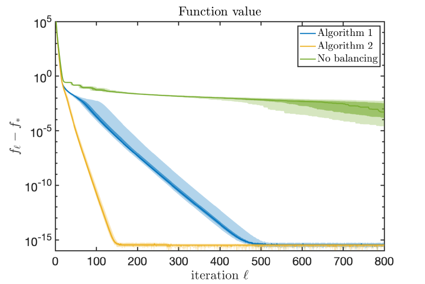
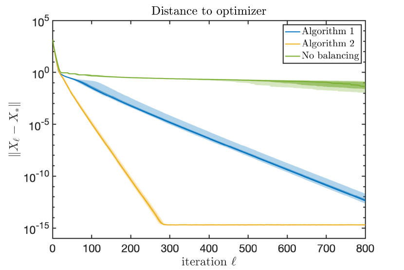
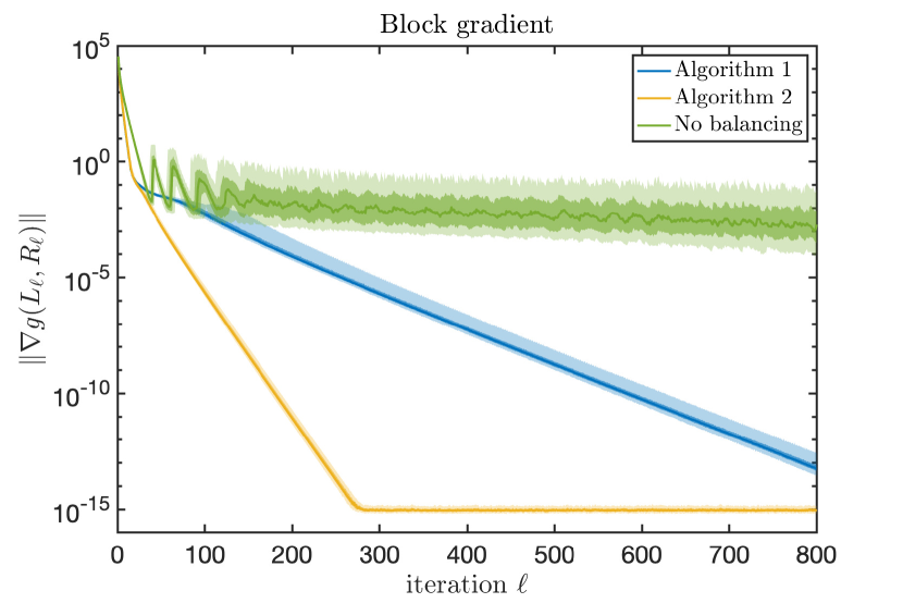
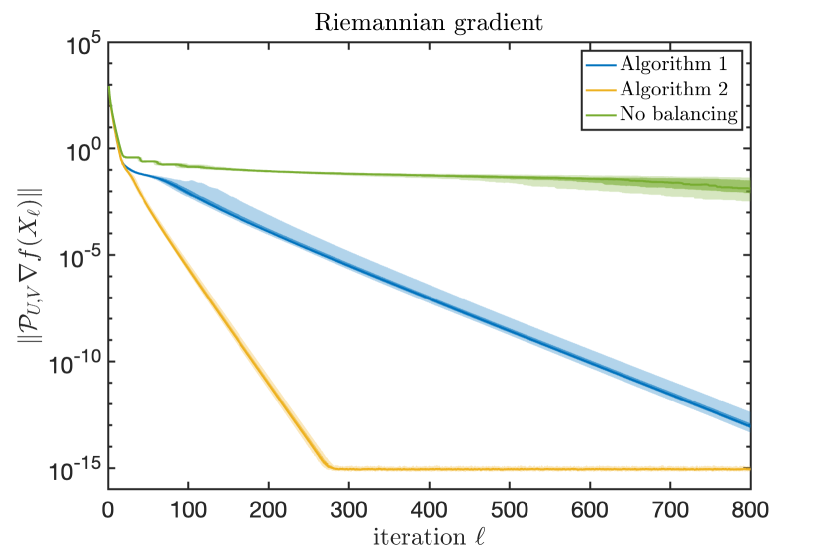
Figure 1: Strongly convex quadratic function with condition number $\kappa_{A}=20$. The effective condition number of the minimizer $X_{*}$ is $\kappa_{X}=5$. The shaded areas correspond to the 50 and 90 percentiles of the relevant quantity in each panel.

Influence of condition numbers $\kappa_{X}$ and $\kappa_{A}$.

As next experiment, we vary the condition numbers $\kappa_{A}$ and $\kappa_{X}$. We no longer report on the version of Algorithm 1 without balancing since it is clearly inferior. The size $n=30$ and rank $k=8$ is the same as above, and we take again 100 random realizations.

In Figure 2, the condition number $\kappa_{A}=20$ of $f$ is kept the same but the effective condition number $\kappa_{X}$ of the rank $k=8$ minimizer $X_{*}$ is varied from $1.1$ to $100$. We clearly see that the Riemannian Algorithm 2 is mostly unaffected by changes in $\kappa_{X}$, whereas the convergence for balancing (Algorithm 1) deteriorates with increasing $\kappa_{X}$. Quite remarkably, for $\kappa_{X}=1$ (not shown) both algorithms have essentially the same convergence behavior. For $\kappa_{X}=1.1$ already, Algorithm 1 is slightly slower than Algorithm 2. We can thus conclude that for this problem Algorithm 1 is not robust with respect to the smallest singular values in $X_{*}$. Algorithm 2 however is robust.

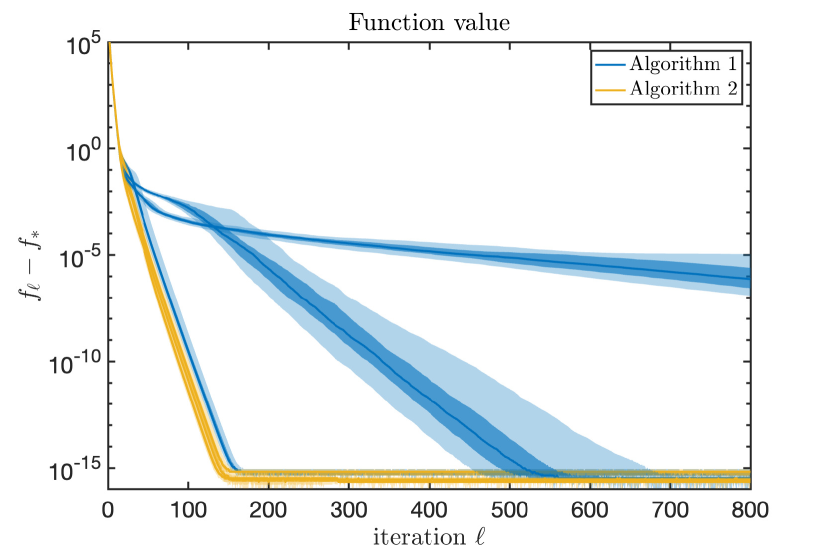
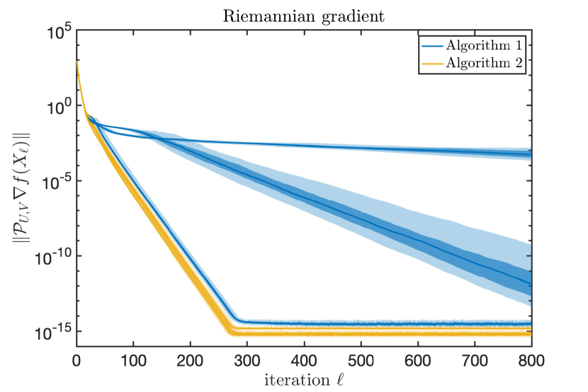
Figure 2: Same setting as Fig. 1 but now with several values of $\kappa_{X}\in\{1.1,10,100\}$. The shaded areas correspond from left to right to increasing values of $\kappa_{X}$.

As related experiment, we now keep $\kappa_{X}$ fixed but vary the condition number $\kappa_{A}$ of $f$. In this case, it is normal that any algorithm that uses only first-order information will converge slower with higher $\kappa_{A}$. Instead of a figure, Table 1 lists the iteration numbers needed to achieve a reduction of the relative error in function value below a fixed tolerance of $\tau=10^{-10}$. In particular, for 100 random realizations of $f$ with the same $\kappa_{X}$, we compute the median of

$$\ell_{\tau}=\min\left\{\ell\in\mathbb{N}\ \colon\ \frac{f(X_{\ell})-f(X_{*})}{f(X_{0})-f(X_{*})}<\tau\right\}.$$

	$\kappa_{A}$	1	10	1000
$\kappa_{X}=1$	Alg. 1	$12\pm 1.5$	$25\pm 4.5$	$98\pm 30$
	Alg. 2	$3\pm 0$	$18\pm 1$	$85\pm 6.5$
$\kappa_{X}=5$	Alg. 1	$20\pm 4.5$	$45\pm 10$	$142\pm 23$
	Alg. 2	$3\pm 0$	$18\pm 1$	$81\pm 6$

Table 1: Number of iterations $\ell_{\tau}$ needed to reduce the relative error in function value to at least $10^{-10}$. The first number shows the median over 100 random realizations and the second number is half the width of the 90 percentile interval.

Influence of line search.

Since the experiments from above all used exact line searches, we also tested fixed step sizes and Armijo backtracking. The experimental results are visible in Figure 3.

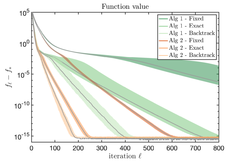
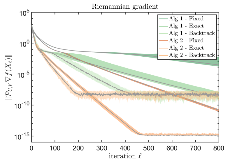
Figure 3: Influence of the line search for a strongly convex quadratic function with fixed condition numbers $\kappa_{A}=40$ and $\kappa_{X}=5$. The colored shaded areas correspond to the 90 percentile data over 20 random realizations. The grey lines indicate the median values.

For the Armijo step-size rule, we use backtracking with the following parameters as defined in Theorems 3.1 and 3.4: initial step size $h_{0}=10$, step reduction factor $\beta=0.5$, and sufficient decrease factor $\gamma=10^{-4}$. For the exact step size, we use $\alpha_{\ell}=0.5$ in Theorems 3.1 and 3.4. In addition, for the radius $\rho$ needed in Theorem 3.1 we take $\|X_{\ell}\|_{2}$. While this is not practical, it gives the best performance for Algorithm 1.

As expected, the fixed step-size rules lead to the slowest convergence since they are based on the worst case global Lipschitz constant. Rather surprising, the Armijo step-size rule has the fastest convergence in terms of iterations. However, it needs on average about 10 function evaluations per iteration (but this can likely be improved with more advanced line searches based on interpolation and warm starting). On the other hand, the exact line search is only feasible for some problems like quadratic functions. Moreover, Armijo backtracking cannot decrease the Riemannian gradient much beyond the square root $\sqrt{\varepsilon_{\text{mach}}}$ of the machine precision. This is a well-known problem due to roundoff error when testing the sufficient decrease condition in finite precision (but it could be mitigated to some extent by the techniques from [21]). Finally, we see that for each choice of line search, Algorithm 1 is slower than Algorithm 2.

In summary, our experiments confirm several indications from the theoretical analysis that the Riemannian version of the Gauss–Southwell selection rule as realized by Algorithm 2 is superior to the factorized version based on balancing (Algorithm 1). This concerns the convergence rates as well as robustness against small singular values.

Acknowledgements

We thank P.-A. Absil for valuable discussion on several parts of this work. The work of G.O. was supported by the Fonds de la Recherche Scientifique – FNRS and the Fonds Wetenschappelijk Onderzoek – Vlaanderen under EOS Project no 30468160 and by the Fonds de la Recherche Scientifique – FNRS under Grant no T.0001.23. The work of A.U. was supported by the Deutsche Forschungsgemeinschaft (DFG, German Research Foundation) – Projektnummer 506561557. The work of B.V. was supported by the Swiss National Science Foundation (grant number 192129).

References

• [1] P.-A. Absil and K. A. Gallivan. Accelerated line-search and trust-region methods. SIAM J. Numer. Anal., 47(2):997–1018, 2009.
• [2] P.-A. Absil, R. Mahony, and R. Sepulchre. Optimization algorithms on matrix manifolds. Princeton University Press, Princeton, NJ, 2008.
• [3] J. Harris. Algebraic geometry: A first course. Springer-Verlag, New York, 1992.
• [4] S. Hosseini, D. R. Luke, and A. Uschmajew. Tangent and normal cones for low-rank matrices. In Nonsmooth optimization and its applications, pages 45–53. Birkhäuser/Springer, Cham, 2019.
• [5] E. Levin, J. Kileel, and N. Boumal. The effect of smooth parametrizations on nonconvex optimization landscapes. arXiv:2207.03512, 2022.
• [6] E. Levin, J. Kileel, and N. Boumal. Finding stationary points on bounded-rank matrices: a geometric hurdle and a smooth remedy. Math. Program., 199(1-2, Ser. A):831–864, 2023.
• [7] Q. Li, Z. Zhu, and G. Tang. The non-convex geometry of low-rank matrix optimization. Inf. Inference, 8(1):51–96, 2019.
• [8] X. Li, Z. Zhu, A. M.-C. So, and R. Vidal. Nonconvex robust low-rank matrix recovery. SIAM J. Optim., 30(1):660–686, 2020.
• [9] D. G. Luenberger and Y. Ye. Linear and nonlinear programming. Springer, Cham, fifth edition, 2021.
• [10] Y. Luo, X. Li, and A. R. Zhang. On geometric connections of embedded and quotient geometries in Riemannian fixed-rank matrix optimization. arXiv:2110.12121, 2021.
• [11] Z. Q. Luo and P. Tseng. On the convergence of the coordinate descent method for convex differentiable minimization. J. Optim. Theory Appl., 72(1):7–35, 1992.
• [12] B. Mishra, K. Adithya Apuroop, and R. Sepulchre. A Riemannian geometry for low-rank matrix completion. arXiv:1211.1550, 2012.
• [13] Y . Nesterov. Efficiency of coordinate descent methods on huge-scale optimization problems. SIAM J. Optim., 22(2):341–362, 2012.
• [14] Y. Nesterov. Lectures on convex optimization. Springer, Cham, 2018.
• [15] J. Nutini, M. Schmidt, I. Laradji, M. Friedlander, and H. Koepke. Coordinate descent converges faster with the Gauss–Southwell rule than random selection. In Proceedings of the 32nd International Conference on Machine Learning, pages 1632–1641. PMLR, 2015.
• [16] G. Olikier and P.-A. Absil. An apocalypse-free first-order low-rank optimization algorithm with at most one rank reduction attempt per iteration. arXiv:2208.12051, 2022.
• [17] G. Olikier and P.-A. Absil. On the continuity of the tangent cone to the determinantal variety. Set-Valued Var. Anal., 30(2):769–788, 2022.
• [18] Y. Saad. Iterative methods for linear systems of equations: a brief historical journey. In 75 years of mathematics of computation, pages 197–215. Amer. Math. Soc., [Providence], RI, 2020.
• [19] R. Schneider and A. Uschmajew. Convergence results for projected line-search methods on varieties of low-rank matrices via Łojasiewicz inequality. SIAM J. Optim., 25(1):622–646, 2015.
• [20] R. Sun and Z.-Q. Luo. Guaranteed matrix completion via non-convex factorization. IEEE Trans. Inform. Theory, 62(11):6535–6579, 2016.
• [21] M. Sutti and B. Vandereycken. Riemannian multigrid line search for low-rank problems. SIAM J. Sci. Comput., 43(3):A1803–A1831, 2021.
• [22] J. Tanner and K. Wei. Low rank matrix completion by alternating steepest descent methods. Appl. Comput. Harmon. Anal., 40(2):417–429, 2016.
• [23] T. Tong, C. Ma, and Y. Chi. Accelerating ill-conditioned low-rank matrix estimation via scaled gradient descent. J. Mach. Learn. Res., 22(150):1–63, 2021.
• [24] Z. Zhu, Q. Li, G. Tang, and M. B. Wakin. Global optimality in low-rank matrix optimization. IEEE Trans. Signal Process., 66(13):3614–3628, 2018.
• [25] Z. Zhu, Q. Li, G. Tang, and M. B. Wakin. The global optimization geometry of low-rank matrix optimization. IEEE Trans. Inform. Theory, 67(2):1308–1331, 2021.