Boundary conditions and universal finite-size scaling
for the hierarchical $|\varphi|^{4}$ model in dimensions 4 and higher

Abstract

We analyse and clarify the finite-size scaling of the weakly-coupled hierarchical $n$-component $|\varphi|^{4}$ model for all integers $n\geq 1$ in all dimensions $d\geq 4$, for both free and periodic boundary conditions. For $d>4$, we prove that for a volume of size $R^{d}$ with periodic boundary conditions the infinite-volume critical point is an effective finite-volume critical point, whereas for free boundary conditions the effective critical point is shifted smaller by an amount of order $R^{-2}$. For both boundary conditions, the average field has the same non-Gaussian limit within a critical window of width $R^{-d/2}$ around the effective critical point, and in that window we compute the universal scaling profile for the susceptibility. In contrast, and again for both boundary conditions, the average field has a massive Gaussian limit when above the effective critical point by an amount $R^{-2}$. In particular, at the infinite-volume critical point the susceptibility scales as $R^{d/2}$ for periodic boundary conditions and as $R^{2}$ for free boundary conditions. We identify a mass generation mechanism for free boundary conditions that is responsible for this distinction and which we believe has wider validity, in particular to Euclidean (non-hierarchical) models on $\mathbb{Z}^{d}$ in dimensions $d\geq 4$. For $d=4$ we prove a similar picture with logarithmic corrections. Our analysis is based on the rigorous renormalisation group method of Bauerschmidt, Brydges and Slade, which we improve and extend.

1 Introduction and main results

1.1 Critical behaviour of the $|\varphi|^{4}_{4}$ model

The $\varphi^{4}$ model on the Euclidean lattice $\mathbb{Z}^{d}$ is a close relative of the Ising model and has been studied for decades as one of the most fundamental spin models in statistical mechanics and Euclidean quantum field theory [39, 33]. Given $n\in\mathbb{N}$, $g>0$, $\nu\in\mathbb{R}$, a finite set $\Lambda\subset\mathbb{Z}^{d}$, and a spin field $\varphi:\Lambda\to\mathbb{R}^{n}$, the finite-volume $|\varphi|^{4}$ Hamiltonian is

$$H(\varphi)=\frac{1}{2}(\varphi,(-\Delta)\varphi)+\sum_{x\in\Lambda}\Big{(}\frac{1}{4}g|\varphi_{x}|^{4}+\frac{1}{2}\nu|\varphi_{x}|^{2}\Big{)}.$$ (1.1)

Our interest here is the theory’s critical behaviour, which occurs for $\nu$ at and near a critical value $\nu_{c}$ which is negative and corresponds to a specific double-well potential when $n=1$. Recent advances include a proof that the spontaneous magnetisation vanishes at the critical point in all dimensions $d\geq 3$ [40], and a proof of the critical theory’s Gaussian nature in the upper critical dimension $d=4$ [2] following a long history for dimensions $d\geq 4$ [1, 4, 36] which in particular established mean-field critical behaviour for $d>4$. The critical scaling and logarithmic corrections to mean-field behaviour at the upper critical dimension $d=4$ also have a long history via rigorous renormalisation group (RG) analysis in the case of weak coupling, as we discuss in detail in Section 1.4.1.

Finite-size scaling in dimensions $d\geq 4$ has been widely discussed in the physics literature, both via scaling arguments and numerical simulations (e.g., [12, 27, 51, 52, 62, 63]), and it is desirable to have rigorous results which specify the behaviour definitively. Our purpose here is to analyse the critical finite-size scaling of the weakly-coupled $n$-component $|\varphi|^{4}$ model in dimensions $d\geq 4$, to indicate the differing effects of free boundary conditions (FBC) vs periodic boundary conditions (PBC), to elucidate the universal scaling profile in the vicinity of the effective finite-volume critical point (sometimes called a pseudocritical point), and to compute the logarithmic corrections present for $d=4$.

Following a long tradition in rigorous RG analysis going back to Dyson [28], we work with the $d$-dimensional hierarchical model rather than the Euclidean lattice $\mathbb{Z}^{d}$, which provides for a simpler analysis yet still exhibits behaviour which we believe to apply exactly also for $\mathbb{Z}^{d}$. Among the copious previous work on hierarchical models, we mention [37, 41, 8, 16, 17, 59, 13]. Hierarchical models have also recently attracted attention in percolation theory, e.g., [43, 44]. Our approach is based on the rigorous RG method of the $4$-dimensional hierarchical $|\varphi|^{4}$ model in [8], which we improve and extend in order to apply it to the finite-size scaling. We also extend the method to apply to dimensions $d>4$. This RG method is inspired by Wilson’s progressive integration over scales, but with no uncontrolled approximations.

Finite-size scaling has a long history in physics, which is natural given that laboratory systems are finite by definition. Numerical simulations of course also involve only finite systems, and finite-size effects are important for the interpretation of simulation data. The early history of finite-size scaling is summarised in [22], an introduction is provided in [21, Section 4.4], and an extensive account is given in [64, Chapter 32]. In brief, the physics picture is as follows:

• The exact critical point for an infinite system is replaced by a critical window whose size scales with the volume $\Lambda$ as $|\Lambda|^{-\theta}$ with window or rounding exponent $\theta$, and with a logarithmic correction at the upper critical dimension.

• Within the critical window, the scaling of the susceptibility and other moments of the average field is governed by universal profiles.

• The location of the critical window is affected by FBC vs PBC.

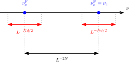
(a) $d>4$.

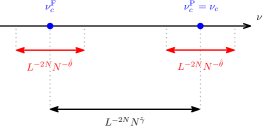
(b) $d=4$.

Figure 1.1: Effective critical points $\nu_{c}^{\rm F}$, $\nu_{c}^{\rm P}$ and scaling windows (red) for FBC and PBC for (a) $d>4$ and (b) $d=4$. The scaling windows for FBC and PBC do not overlap. At the infinite-volume critical point $\nu_{c}$, the average field has a Gaussian limit with FBC and a non-Gaussian limit with PBC.

Our results give a complete description of the above three points for the weakly-coupled hierarchical $|\varphi|^{4}$ model in a finite volume $\Lambda_{N}$ of size $L^{dN}$, in dimensions $d\geq 4$, with $L$ fixed and $N$ large. A summary is given in Figure 1.1. We write the average field as $\Phi_{N}=L^{-dN}\sum_{x\in\Lambda_{N}}\varphi_{x}$.

For $d>4$, we prove that for all $n\geq 1$:

• For PBC, there is a critical window of width $L^{-Nd/2}$ containing the infinite-volume critical point $\nu_{c}$, within which the rescaled average field $L^{Nd/4}\Phi_{N}$ converges to a non-Gaussian distribution with density proportional to $e^{-\frac{1}{4}|x|^{4}-\frac{1}{2}s|x|^{2}}$. The variable $s\in(-\infty,\infty)$ parametrises the location within the critical window. We explicitly compute the universal profiles of the susceptibility and other moments of the average field within the window. Within the window, the susceptibility scales as $L^{Nd/2}$.

• For FBC, the effective critical point is not $\nu_{c}$ (as it is for PBC) but instead is shifted smaller to $\nu_{c}-\Theta(L^{-2N})$. Around this shifted effective critical point there is again a critical window of width $L^{-Nd/2}$ within which the average field and the susceptibility scale exactly as they do for PBC, with the same universal profiles.

• For both FBC and PBC, when $\nu$ is above the effective critical point by an amount $sL^{-2N}$ with $s>0$, the rescaled average field $L^{N(d-2)/2}\Phi_{N}$ converges to a Gaussian distribution with density proportional to $e^{-\frac{1}{2}s|x|^{2}}$. The susceptibility scales as $L^{2N}$. For FBC, the infinite-volume critical point $\nu_{c}$ lies in this Gaussian range and hence the susceptibility at $\nu_{c}$ scales as $L^{2N}$, unlike for PBC where the scaling is $L^{Nd/2}$.

For $d=4$, let

$$\hat{\gamma}=\frac{n+2}{n+8},\qquad\hat{\theta}=\frac{4-n}{2(n+8)}=\frac{1}{2}-\hat{\gamma}.$$ (1.2)

We prove that the $d>4$ picture applies also for $d=4$ but with logarithmic corrections (polynomial in $N$) for all $n\geq 1$:

• For PBC, there is a critical window of width $L^{-2N}N^{-\hat{\theta}}$ containing the infinite-volume critical point $\nu_{c}$, within which the rescaled average field $N^{1/4}L^{N}\Phi_{N}$ converges to a non-Gaussian distribution with density proportional to $e^{-\frac{1}{4}|x|^{4}-\frac{1}{2}s|x|^{2}}$. The universal profile of the susceptibility and other moments of the average field within the window are identical to those for $d>4$. Within the window the susceptibility scales as $L^{2N}N^{1/2}$.

• For FBC, the effective critical point is shifted smaller to $\nu_{c}-\Theta(L^{-2N}N^{\hat{\gamma}})$. Around this shifted effective critical point there is a critical window of width $L^{-2N}N^{-\hat{\theta}}$ within which the average field, the susceptibility and other moments of the average field scale exactly as they do in the critical window for PBC.

• For both FBC and PBC, above their effective critical points by an amount $sL^{-2N}N^{\hat{\gamma}}$ with $s>0$, the rescaled average field $L^{N}\Phi_{N}$ converges to a Gaussian distribution with density proportional to $e^{-\frac{1}{2}s|x|^{2}}$. The susceptibility scales as $L^{2N}$. For FBC, the infinite-volume critical point $\nu_{c}$ lies in this Gaussian range and hence the susceptibility at $\nu_{c}$ scales as $L^{2N}$, unlike for PBC where the scaling is $L^{2N}N^{1/2}$.

For dimensions $d>4$ (above the upper critical dimension) with PBC, the physics predictions for the universal profile, the window width, and the size of the susceptibility in the window are stated in [64, Section 32.3.1]. For both FBC and PBC in dimensions $d>4$, [35, Table 1] presents predictions which are consistent with our theorems for the scaling of the susceptibility, the scaling of the average field, and the shift in the effective critical point for FBC (see also [12, p.38]). For $d=4$, the physics predictions for the logarithmic correction to the susceptibility and the window size are given in [47, (3.6)] and [47, (4.3)].

Our results provide a rigorous justification of the physics predictions, for the hierarchial lattice in all dimensions $d\geq 4$ and for all $n\geq 1$. Our proof presents a clear mechanism responsible for the shift in the effective critical point for FBC: the free boundary condition generates an effective mass in the Hamiltonian which must be compensated be a shift in the value of $\nu$ to attain effective FBC critical behaviour. In addition, although our results are proved only for the hierarchial model, they lead to precise conjectures for the behaviour for Euclidean models on $\mathbb{Z}^{d}$ for all $d\geq 4$, which we spell out in Section 1.6, not just for the $n$-component $|\varphi|^{4}$ model but also for $O(n)$ models (e.g., Ising, $XY$, Heisenberg models) and self-avoiding walk models ($n=0$).

Notation. We write $f_{N}\sim g_{N}$ to denote $\lim_{N}f_{N}/g_{N}=1$, and use $f_{N}\asymp g_{N}$ or $f_{N}=\Theta(g_{N})$ to denote the existence of $C>0$ such that $C^{-1}g_{N}\leq f_{N}\leq Cg_{N}$.

1.2 The hierarchical Laplacian

The hierarchial $|\varphi|^{4}$ model is defined using the hierarchical Laplacian in the Hamiltonian (1.1). We define the hierarchical Laplacian in this section as the generator for a random walk with FBC or PBC (see also [44] for discussion of hierarchical BC). The definitions in this section apply to any dimension $d\geq 1$. Also, we introduce a parameter $\alpha$ (in (1.7)) even though we only use the case $\alpha=2$, in order to emphasise its role.

1.2.1 The hierarchical group

Given integers $L>1$ and $N\geq 1$, let $\Lambda_{N}$ denote the cube $\Lambda_{N}=\{x\in\mathbb{Z}^{d}:0\leq x_{i}<L^{N}\;\text{for}\;i=1,\ldots,d\}$, which has volume (cardinality) $L^{dN}$. The thermodynamic limit is the limit $N\to\infty$, for which $\Lambda_{\infty}=\{x\in\mathbb{Z}^{d}:0\leq x_{i}\;\text{for}\;i=1,\ldots,d\}$. Given an integer $0\leq j\leq N$, we can partition $\Lambda_{N}$ into $L^{d(N-j)}$ disjoint blocks which are each translates of $\Lambda_{j}$ and which each contain $L^{dj}$ vertices. We denote the set of such $j$-blocks by $\mathcal{B}_{j}$. See Figure 1.2.

Figure 1.2: The block $\Lambda_{3}$ with its blocks in ${\cal B}_{0},{\cal B}_{1},{\cal B}_{2},{\cal B}_{3}$ for the case $d=L=2$.

An equivalent representation of $\Lambda_{\infty}$ is as follows. With $\mathbb{Z}_{L}=\mathbb{Z}/L\mathbb{Z}$ the cyclic group, let

$$\mathbb{H}_{\infty}=\{\tilde{x}=(\tilde{x}_{1},\tilde{x}_{2},\ldots):\text{$\tilde{x}_{i}\in\mathbb{Z}_{L}^{d}$ with only finitely many nonzero $\tilde{x}_{i}$}\}.$$ (1.3)

This is an abelian group with coordinatewise addition mod-$L$; we denote the group addition as $+$. We define $\mathbb{H}_{N}$ to be the subgroup of $\mathbb{H}_{\infty}$ with $\tilde{x}_{i}=0$ for $i>N$. The map $\sigma:\mathbb{H}_{\infty}\to\Lambda_{\infty}$ defined by

$$\sigma(\tilde{x})=\sum_{j=1}^{\infty}L^{j-1}x_{j}$$ (1.4)

is a bijection, where $x_{j}$ is the representative of $\tilde{x}_{j}$ in $\Lambda_{1}\subset\mathbb{Z}^{d}$. Addition on the right-hand side of (1.4) is in $\mathbb{Z}^{d}$. Note that $\sigma$ restricts to a bijection $\sigma_{N}:\mathbb{H}_{N}\to\Lambda_{N}$. The bijection induces an addition and a group structure on $\Lambda_{N}$ via $x\oplus y=\sigma_{N}(\sigma_{N}^{-1}x+\sigma_{N}^{-1}y)$ (with $+$ the addition on $\mathbb{H}_{N}$); this makes $\sigma_{N}$ and $\sigma$ into group isomorphisms.

For $x,y\in\Lambda_{N}$, we define the coalescence scale $j_{xy}$ to be the smallest $j$ such that $x$ and $y$ lie in the same $j$-block. In terms of $\mathbb{H}_{N}$, $j_{xy}$ is the largest coordinate $i$ such that $(\sigma_{N}^{-1}x)_{i}$ differs from $(\sigma_{N}^{-1}y)_{i}$, and from this observation we see that

$$j_{x\oplus z,y\oplus z}=j_{xy}\qquad(x,y,z\in\Lambda_{N}).$$ (1.5)

In particular, with subtraction in $\Lambda_{N}$ denoted by $\ominus$,

$$j_{xy}=j_{0,y\ominus x}\qquad(x,y\in\Lambda_{N}).$$ (1.6)

1.2.2 Hierarchical random walk

Random walk on the infinite hierarchial group. Given $\alpha>0$, we define a discrete-time random walk on the group $\Lambda_{\infty}$ via the transition probabilities

$$J_{xy}=\frac{1}{z}\frac{1}{L^{(d+\alpha)j_{xy}}}\qquad(x,y\in\Lambda_{\infty},\;x\neq y),$$ (1.7)

with the constant $z=z(d,L,\alpha)$ chosen so that $\sum_{x\neq 0}J_{0x}=1$. By (1.6), the transition probabilities are translation invariant in the sense that $J_{x,y}=J_{0,y\ominus x}$. Since the number of sites $x\in\Lambda_{\infty}$ with $j_{0x}=k$ is

$$n_{k}=L^{dk}-L^{d(k-1)}=L^{dk}(1-L^{-d}),$$ (1.8)

the constant $z$ is given by

$$z =\sum_{x\neq 0}L^{-(d+\alpha)j_{0x}}=\sum_{k=1}^{\infty}n_{k}L^{-(d+\alpha)k}=\frac{1-L^{-d}}{L^{\alpha}-1}.$$ (1.9)

Random walk with FBC. We define a random walk on $\Lambda_{N}\times\{\dagger\}$ which is killed when it lands on the cemetery state $\dagger$. The killing occurs when a random walk on the infinite hierarchical lattice $\Lambda_{\infty}$ exits $\Lambda_{N}$ for the first time. This corresponds to FBC. Explicitly, for $x\in\Lambda_{N}$,

$$J^{\rm F}_{x\dagger} =\sum_{y:j_{xy}>N}J_{xy}=\frac{1}{z}\sum_{k=N+1}^{\infty}n_{k}L^{-(d+\alpha)k}=L^{-\alpha N},$$ (1.10)

whereas for $x,y\in\Lambda_{N}$ we maintain the infinite-volume transition probability from (1.7), namely

$$J^{\rm F}_{xy} =z^{-1}L^{-(d+\alpha)j_{xy}}\qquad(x,y\in\Lambda_{N},\;x\neq y).$$ (1.11)

This produces a defective (unnormalised) distribution $J^{\rm F}$ on $\Lambda_{N}$ for which

$$\sum_{x\in\Lambda_{N}}J^{\rm F}_{0x}=1-L^{-\alpha N}.$$ (1.12)

Random walk with PBC. With $N$ fixed, we define an equivalence relation on $\Lambda_{\infty}$ by $x\sim y$ if $\tilde{x}_{i}=\tilde{y}_{i}$ for $i=1,\ldots,N$, where $\tilde{x}=\sigma^{-1}x$, $\tilde{y}=\sigma^{-1}y$. The quotient space $\Lambda_{\infty}/\!\!\sim$ can be identified with $\Lambda_{N}$. The random walk on $\Lambda_{\infty}$ with transition matrix (1.7) projects via the quotient map to a random walk on $\Lambda_{N}$. This projection corresponds to PBC. Explicitly, since for $k>N$ the block $\Lambda_{k}$ contains exactly $n_{k}L^{-dN}$ points with $j_{0x}=k$ that are equivalent to $y\in\Lambda_{N}$, for the same normalising constant $z$ as in (1.9) the quotient walk has transition probabilities

$$J^{\rm P}_{xy} =\frac{1}{z}L^{-(d+\alpha)j_{xy}}+L^{-dN}\sum_{k=N+1}^{\infty}n_{k}\frac{1}{z}L^{-(d+\alpha)k}$$

$$=\frac{1}{z}L^{-(d+\alpha)j_{xy}}+{L^{-(d+\alpha)N}}\qquad(x,y\in\Lambda_{N},\;x\neq y).$$ (1.13)

1.2.3 The hierarchical Laplacian with boundary conditions

In general, given a transition matrix $J_{xy}$ (defective or not), we define a Laplacian by $-\tilde{\Delta}=1-J$ and we let $-\tilde{\Delta}$ act on an $n$-component spin field $\varphi:\Lambda_{N}\to\mathbb{R}^{n}$ component-wise. Here $1$ denotes the identity matrix. If $J$ is defective then the Laplacian is massive (i.e., has a spectral gap), and otherwise it is massless. For the $|\varphi|^{4}$ model, the critical behaviour is not affected by replacing the Laplacian term in the Hamiltonian by a multiple of the Laplacian. We use this flexibility in the following definitions in order to achieve coherence between our Laplacian with PBC and the hierarchial Laplacian defined in [8, Definition 4.1.7]. Since the random walks with FBC and PBC are translation invariant (with respect to $\oplus$) by definition, the Laplacians they define obey

$$\tilde{\Delta}_{xy}=\tilde{\Delta}_{0,y\ominus x}\qquad(x,y\in\Lambda_{N}).$$ (1.14)

In particular, it suffices to specify the matrix elements $\tilde{\Delta}_{0x}$ to define the Laplacians.

For $*={\rm P,F}$, and with $J^{*}$ the matrix of transition probabilities with boundary condition $*$, we define

$$-\tilde{\Delta}^{*} =1-J^{*}.$$ (1.15)

For $x,y\in\Lambda_{N}$ we define $Q_{N:xy}=L^{-dN}$. It follows from the definitions of $J^{*}$ that

$$1-J^{\rm F} =1-J^{\rm P}+L^{-\alpha N}Q_{N}.$$ (1.16)

The matrix $-\tilde{\Delta}^{\rm P}$ obeys $\sum_{x\in\Lambda_{N}}(1-J^{\rm P})_{0x}=0$, whereas $-\tilde{\Delta}^{\rm F}$ obeys $\sum_{x\in\Lambda_{N}}(1-J^{\rm F})_{0x}=L^{-\alpha N}$.

Multiplication of the Laplacian by a scalar amounts to a rescaling of the field. We do the rescaling in the same way for both boundary conditions, by defining

$$-\Delta^{*} =q(-\tilde{\Delta}^{*})=q(1-J^{*})$$ (1.17)

with

$$q=\frac{1-L^{-d}}{1-L^{-(d+\alpha)}}.$$ (1.18)

With this definition, $\Delta^{{\rm P}}$ is exactly the Laplacian in [8, Definition 4.1.7], as we indicate in Section 2.1. By (1.16),

$$-\Delta^{\rm F} =-\Delta^{\rm P}+qL^{-\alpha N}Q_{N}.$$ (1.19)

The Green function (inverse Laplacian) on $\Lambda_{\infty}$ obeys

$$(-\Delta)^{-1}_{0x}\asymp|x|^{-(d-\alpha)}\qquad(0<\alpha<d),$$ (1.20)

with $|x|$ the Euclidean norm; the proof given in [8, (4.1.29)] for $\alpha=2$ applies also for $0<\alpha<d$. For $\alpha=2$, the right-hand side of (1.20) is the decay of the Green function for the standard nearest-neighbour Laplacian on $\mathbb{Z}^{d}$. This indicates a close connection between the hierarchical Laplacian and the Euclidean Laplacian.

1.3 The hierarchical $|\varphi|^{4}$ model

Let $-\Delta^{*}$ represent either $-\Delta^{{\rm F}}$ or $-\Delta^{{\rm P}}$ on $\Lambda_{N}$, so that either boundary condition can be used in the following definitions. We always take $\alpha=2$ in the definition of the Laplacian. Given $n\in\mathbb{N}$, $g>0$, $\nu\in\mathbb{R}$, and a spin field $\varphi:\Lambda_{N}\to\mathbb{R}^{n}$, we define the hierarchical Hamiltonian

$$H_{\nu,N}^{*}(\varphi)=\frac{1}{2}(\varphi,(-\Delta^{*})\varphi)+\sum_{x\in\Lambda_{N}}\Big{(}\frac{1}{4}g|\varphi_{x}|^{4}+\frac{1}{2}\nu|\varphi_{x}|^{2}\Big{)},$$ (1.21)

the partition function

$$Z_{\nu,N}^{*}=\int_{(\mathbb{R}^{n})^{\Lambda_{N}}}e^{-H_{\nu,N}^{*}(\varphi)}d\varphi,$$ (1.22)

and the associated expectation

$$\langle F\rangle_{\nu,N}^{*}=\frac{1}{Z_{\nu,N}^{*}}\int_{(\mathbb{R}^{n})^{\Lambda_{N}}}F(\varphi)e^{-H_{\nu,N}^{*}(\varphi)}d\varphi.$$ (1.23)

In (1.21), and in what follows, we use the notation $(\varphi,\psi)=\sum_{x\in\Lambda_{N}}\varphi_{x}\cdot\psi_{x}$, where the dot product is for $\mathbb{R}^{n}$. Also, $|\varphi_{x}|=(\varphi_{x}\cdot\varphi_{x})^{1/2}$ denotes the Euclidean norm of $\varphi_{x}\in\mathbb{R}^{n}$. The definitions (1.21)–(1.23) depend on $g$ but since we regard $g$ as fixed (and small) in the following, we do not make this dependence explicit. We will however be interested in varying $\nu$. By definition, the distribution of the field $\varphi$ under (1.23) is invariant under the map $(\varphi_{x})_{x\in\Lambda_{N}}\mapsto(R\varphi_{x})_{x\in\Lambda_{N}}$ for any orthogonal transformation $R\in O(n)$.

Our main objects of study are the distribution of the average field

$$\Phi_{N}=\frac{1}{L^{dN}}\sum_{x\in\Lambda_{N}}\varphi_{x}\in\mathbb{R}^{n}$$ (1.24)

and the expectations $\langle|\Phi_{N}|^{2p}\rangle_{\nu,N}$ for $p\in\mathbb{N}$. An important special case is $2p=2$, the finite-volume susceptibility:

$$\chi_{N}^{*}(\nu)=\sum_{x\in\Lambda_{N}}\langle\varphi_{0}^{(1)}\varphi_{x}^{(1)}\rangle_{\nu,N}^{*}=\frac{1}{n}\sum_{x\in\Lambda_{N}}\langle\varphi_{0}\cdot\varphi_{x}\rangle_{\nu,N}^{*}=\frac{|\Lambda_{N}|}{n}\langle|\Phi_{N}|^{2}\rangle_{\nu,N}^{*},$$ (1.25)

where $\varphi_{x}^{(j)}$ denotes the $j^{\rm th}$ component of $\varphi_{x}\in\mathbb{R}^{n}$. The second equality of (1.25) is a consequence of the $O(n)$ invariance. The third follows from the fact that, by (1.14), under the probability measure given by (1.23) the pair $(\varphi_{x},\varphi_{y})$ has the same distribution as $(\varphi_{0},\varphi_{y\ominus x})$ for any $x,y\in\Lambda_{N}$, so $(\varphi_{x},\Phi_{N})$ and $(\varphi_{y},\Phi_{N})$ have the same distribution too. The susceptibility is more naturally defined using a truncated expectation in which the square of the infinite-volume spontaneous magnetisation is subtracted from the expectation $\langle\varphi_{0}\cdot\varphi_{x}\rangle_{\nu,N}$. We discuss the distinction between these two definitions in more detail at the end of Section 1.5.1.

1.4 Main results

Our main results are valid in all dimensions $d\geq 4$ and for all $n\geq 1$. They are of three types:

1. In Theorem 1.1, we identify the infinite-volume critical point $\nu_{c}$, and for $\nu=\nu_{c}+\varepsilon$ with $\varepsilon>0$ fixed, we prove a Gaussian limit theorem for the average field, and compute moments of the average field. In this limit theorem, the average field is scaled by $L^{Nd/2}$ (Gaussian scaling). The results apply for both FBC and PBC, and there are logarithmic corrections for $d=4$.

2. In Theorem 1.2, we identify effective finite-volume critical points $\nu_{c,N}^{*}$ for FBC and PBC, with $\nu_{c,N}^{\rm P}=\nu_{c}$, and with $\nu_{c,N}^{\rm F}=\nu_{c}-\Theta(L^{-2N})$ for $d>4$ and $\nu_{c,N}^{\rm F}=\nu_{c}-\Theta(N^{\frac{n+2}{n+8}}L^{-2N})$ for $d=4$. We prove a non-Gaussian limit for the average field for $\nu=\nu_{c,N}^{*}+sw_{N}$ for $s\in(-\infty,\infty)$, where the window scale $w_{N}$ is of order $L^{-Nd/2}$ for $d>4$ and of order $N^{\frac{4-n}{n+8}}L^{-2N}$ for $d=4$. The average field is scaled by $L^{Nd/4}$ for $d>4$ and by $N^{-1/4}L^{N}$ for $d=4$ (non-Gaussian scaling for all $d\geq 4$). Universal profiles for the moments of the average field are identified, and there is a logarithmic correction when $d=4$. The same non-Gaussian limit applies for both FBC and PBC, and the FBC and PBC windows do not overlap.

3. In Theorem 1.3, for FBC and PBC we prove a Gaussian limit for the average field for $\nu=\nu_{c,N}^{*}+sv_{N}$ with $s\in(0,\infty)$, where $v_{N}$ is of order $L^{-2N}$ for $d>4$ and of order $N^{\frac{n+2}{n+8}}L^{-2N}$ for $d=4$. The field is scaled by $L^{N(d-2)/2}$ for all $d\geq 4$, which is non-Gaussian scaling. Theorem 1.3 probes the vicinity of the critical point on a finer scale than Theorem 1.1, but on a scale that is less fine than Theorem 1.2.

The proofs of the three theorems are given in the bulk of the paper.

1.4.1 Gaussian limit and critical behaviour

The following theorem identifies a critical point $\nu_{c}$, for large $L$ and for small $g>0$, at which the infinite-volume hierarchial susceptibility diverges. The restriction to large $L$ is an artifact of the proof and we believe the theorem remains true without it. The theorem also describes the manner of the susceptibility’s divergence. For $d=4$ the theorem is partly proved in [8, Theorem 4.2.1], and we adapt that proof here to include dimensions $d>4$. For the statement of the theorem, for $s>0$ we define a Gaussian measure on $\mathbb{R}^{n}$, together with its moments, by

$$d\mu_{n,s}=\frac{e^{-\frac{1}{2}s|x|^{2}}dx}{\int_{\mathbb{R}^{n}}e^{-\frac{1}{2}s|x|^{2}}dx},\qquad M_{n,k}(s)=\int_{\mathbb{R}^{n}}|x|^{k}d\mu_{n,s}.$$ (1.26)

Theorem 1.1.

(Massive Gaussian limit.) Let $d\geq 4$, let $n\in\mathbb{N}$, let $L$ be sufficiently large, and let $g>0$ be sufficiently small (depending on $L$). There is a critical value $\nu_{c}\in\mathbb{R}$ (depending on $d,n,g,L$), constants $A_{d}$ (depending on $d,g,n,L$), and a strictly positive continuously differentiable function $m_{\varepsilon}^{2}$ defined for all $\varepsilon>0$ with

$$m^{2}_{\varepsilon}\sim\begin{cases}A_{4}^{-1}\,\varepsilon\,(\log\varepsilon^{-1})^{-\hat{\gamma}}&(d=4)\\ A_{d}^{-1}\,\varepsilon&(d>4)\end{cases}\qquad\text{as }\varepsilon\downarrow 0,$$ (1.27)

with $\hat{\gamma}$ given by (1.2) such that the following infinite-volume limits exist for $\varepsilon>0$ and have the values indicated, independent of the boundary condition $*={\rm F}$ or $*={\rm P}$:

1. For any $J\in\mathbb{R}^{n}$,

   $$\lim_{N\to\infty}\langle e^{J\cdot\Phi_{N}L^{Nd/2}}\rangle_{\nu_{c}+\varepsilon,N}^{*}=\int_{\mathbb{R}^{n}}e^{J\cdot x}d\mu_{n,m^{2}_{\varepsilon}}.$$ (1.28)

2. For $p\in\mathbb{N}$,

   $$\lim_{N\to\infty}L^{dNp}\langle|\Phi_{N}|^{2p}\rangle_{\nu_{c}+\varepsilon,N}^{*}=M_{n,2p}(m^{2}_{\varepsilon}).$$ (1.29)

Also, as $g\downarrow 0$, the amplitude in (1.27) and the critical point satisfy

$$A_{4} \sim\Big{(}\frac{(n+8)(1-L^{-d})g}{\log L^{2}}\Big{)}^{\hat{\gamma}},\quad A_{d}=1+O(g)\;\;\;(d>4),\quad\nu_{c}\sim-(n+2)g(-\Delta_{H})^{-1}_{00},$$ (1.30)

with $(-\Delta_{H})^{-1}_{00}$ the diagonal matrix element of the Green function of the infinite-volume hierarchical Laplacian.

Equation (1.28) states that the total field $\sum_{x\in\Lambda_{N}}\varphi_{x}$, after a Gaussian rescaling $L^{-Nd/2}$, converges in distribution under $\langle\,\cdot\,\rangle_{\nu_{c}+\varepsilon,N}$ to a Gaussian random variable with mean zero and variance $1/m^{2}_{\varepsilon}$. The moments in (1.29) can be explicitly evaluated, so that for $p\geq 1$, $\varepsilon>0$, and $*={\rm F}$ or $*={\rm P}$,

$$\lim_{N\to\infty}L^{dNp}\langle|\Phi_{N}|^{2p}\rangle_{\nu_{c}+\varepsilon,N}^{*}=\left(\frac{2}{m^{2}_{\varepsilon}}\right)^{p}\frac{\Gamma(\frac{n+2p}{2})}{\Gamma(\frac{n}{2})}.$$ (1.31)

By the definition of the susceptibility in (1.25), together with (1.27) and the $p=1$ case of (1.31), the infinite-volume susceptibility $\chi_{\infty}$ obeys

$$\chi_{\infty}(\nu_{c}+\varepsilon)=\frac{1}{m_{\varepsilon}^{2}}\sim\begin{cases}A_{4}\,\varepsilon^{-1}\big{(}\log\varepsilon^{-1}\big{)}^{\hat{\gamma}}&(d=4)\\ A_{d}\,\varepsilon^{-1}&(d>4)\end{cases}\qquad\text{as }\varepsilon\downarrow 0,$$ (1.32)

which for $d=4$ recovers [8, Theorem 4.2.1].

The asymptotic formula (1.32) has been proved also for the $|\varphi|^{4}$ model on the Euclidean lattice $\mathbb{Z}^{4}$, with different amplitude $A_{4}\sim[(n+8)g/(16\pi^{2})]^{\hat{\gamma}}$, as part of a large RG literature for weakly-coupled $\varphi^{4}$ models on $\mathbb{Z}^{4}$. For $1$-component spins, it has been proved that the critical two-point function decays as $\langle\varphi_{0}\varphi_{x}\rangle\sim|x|^{-2}$ [38, 32, 58], that the susceptibility and correlation length have logarithmic corrections $\chi\sim\varepsilon^{-1}|\log\varepsilon|^{1/3}$ and $\xi\sim\varepsilon^{-1/2}|\log\varepsilon|^{1/6}$ [42], and that the critical magnetisation vanishes with the magnetic field $h$ as $M\sim h^{1/3}|\log h|^{1/3}$ [50]. For $d=4$ and for general $n\geq 1$, the $|x|^{-2}$ decay of the critical two-point function is proved in [58], the susceptibility and specific heat are proved to obey $\chi\sim\varepsilon^{-1}|\log\varepsilon|^{\frac{n+2}{n+8}}$ and $c_{H}\sim|\log\varepsilon|^{\max\{\frac{4-n}{n+8},0\}}$ ($n\neq 4$) or $c_{H}\sim\log\log\varepsilon^{-1}$ ($n=4$) in [5], and the correlation length of order $p$ is proved to obey $\xi_{p}\sim\varepsilon^{-1/2}|\log\varepsilon|^{\frac{n+2}{2(n+8)}}$ for all $p>0$ [11]. In [6, 7], these asymptotic formulas for the susceptibility and correlation length of order $p$ are extended to $n=0$ which corresponds to the continuous-time weakly self-avoiding walk via an exact supersymmetric representation. Still missing from this catalogue is a proof that the spontaneous magnetisation obeys $M_{+}\sim|\varepsilon|^{1/2}|\log\varepsilon|^{\frac{3}{n+8}}$. Scaling relations among the many logarithmic exponents are presented in [48].

1.4.2 Non-Gaussian limit inside the critical window

To state our results for the non-Gaussian limit, we need several definitions.

The non-Gaussian limiting measure. Given $n\in\mathbb{N}$ and $s\in\mathbb{R}$ we define a non-Gaussian probability measure on $\mathbb{R}^{n}$ and its $k^{\rm th}$ moments ($k>-n$) by

$$d\sigma_{n,s}=\frac{e^{-\frac{1}{4}|x|^{4}-\frac{s}{2}|x|^{2}}dx}{\int_{\mathbb{R}^{n}}e^{-\frac{1}{4}|x|^{4}-\frac{s}{2}|x|^{2}}dx},\qquad\Sigma_{n,k}(s)=\int_{\mathbb{R}^{n}}|x|^{k}d\sigma_{n,s}.$$ (1.33)

The quartic coupling constant. Our RG analysis involves a critical (massless) quartic running coupling constant $g_{j}$ whose value at scale $j=N$ plays an important role. The sequence $g_{j}$ in nonnegative and depends on $g$, $L$, $n$ and $d$. For $d=4$, $g_{N}\sim(BN)^{-1}$, and for $d>4$, $\lim_{N\to\infty}g_{N}=g_{\infty}$. The positive constants $B$ and $g_{\infty}$ are given by

$$B=(n+8)(1-L^{-d}),\qquad g_{\infty}=g+O(g^{2}).$$ (1.34)

We exclude a factor $L^{-(d-4)j}$ from $g_{j}$ for $d>4$; this factor will appear explicitly when appropriate. The fact that $g$ gets renormalised even when $d>4$—the constant $g_{\infty}$ accumulates contributions of all orders—corresponds to the statement that it is a dangerous irrelevant variable as defined in [34].

The window scale. Recall the logarithmic correction exponents $\hat{\gamma}=\frac{n+2}{n+8}$ and $\hat{\theta}=\frac{1}{2}-\hat{\gamma}$ from (1.2), and the constants $A_{d}$ from Theorem 1.1. We define the window scale (or rounding scale)

$$w_{N}=\begin{cases}A_{4}(\log L^{2})^{\hat{\gamma}}B^{-1/2}N^{-\hat{\theta}}L^{-2N}&(d=4)\\ A_{d}\,g_{\infty}^{1/2}L^{-Nd/2}&(d>4).\end{cases}$$ (1.35)

For $d=4$, the factors $(\log L^{2})^{\hat{\gamma}}B^{-1/2}N^{-\hat{\theta}}$ can equivalently be written as the product of $(\log L^{2N})^{\hat{\gamma}}$, which is a correction logarithmic in the volume, multiplied by $(BN)^{-1/2}\sim g_{N}^{1/2}$ which is the $4$-dimensional counterpart of the $g_{\infty}^{1/2}$ appearing for $d>4$. To understand the choice of window scale via a rough computation, for $d>4$ we start with the ansatz $\chi_{N}^{\rm P}(\nu_{c})\asymp L^{Nd/2}$ and choose $w_{N}$ to scale in such a manner that $\chi_{\infty}(\nu_{c}+w_{N})\asymp\chi_{N}^{\rm P}(\nu_{c})$. Since $\chi_{\infty}(\nu_{c}+w_{N})\asymp w_{N}^{-1}$ by (1.32), we conclude that the window should obey $w_{N}\asymp L^{-Nd/2}$ for $d>4$. For $d=4$, similar reasoning leads to $w_{N}\asymp L^{-2N}N^{-\hat{\theta}}$ when we assume that $\chi_{N}^{\rm P}(\nu_{c})\asymp L^{2N}N^{1/2}$ (a prediction of [47] for $\mathbb{Z}^{4}$, which we prove and extend in Corollary 1.4 for the hierarchical model).

The effective critical points. For PBC we define the effective critical point to equal the infinite-volume critical point from Theorem 1.1:

$$\nu^{\rm P}_{c,N}=\nu_{c}.$$ (1.36)

Although $\nu^{\rm P}_{c,N}$ is independent of the volume parameter $N$, we include the subscript to emphasise its role as a finite-volume critical point. For FBC we first define

$$v_{N}=\begin{cases}A_{4}(\log L^{2})^{\hat{\gamma}}N^{\hat{\gamma}}L^{-2N}&(d=4)\\ A_{d}L^{-2N}&(d>4).\end{cases}$$ (1.37)

By definition, $v_{N}$ is much larger than $w_{N}$, namely,

$$v_{N}=\begin{cases}(BN)^{1/2}w_{N}&(d=4)\\ g_{\infty}^{-1/2}L^{N(d-4)/2}w_{N}&(d>4).\end{cases}$$ (1.38)

For FBC, we specify a volume-dependent effective critical point $\nu_{c,N}^{\rm F}$, which we compute exactly when $d=4,5$ and approximately when $d>5$, by

$$\nu_{c,N}^{{\rm F}} =\begin{cases}\nu_{c}-qv_{N}(1+c^{\rm F}N^{-\hat{\gamma}})&(d=4)\\ \nu_{c}-qv_{N}&(d=5)\\ \nu_{c}-qv_{N}(1+O(L^{-N}))&(d>5);\end{cases}$$ (1.39)

here $q=1+O(L^{-d})$ is the constant from (1.18) and $c^{\rm F}=O(g)$ is determined in the proof. The error term $O(L^{-N}v_{N})$ for $d>5$ is the same order as $w_{N}$ for $d=6$ and is larger than $w_{N}$ for $d>6$. Although we do not precisely identify $\nu_{c,N}^{\rm F}$ for $d\geq 6$, we do prove its existence as an anchor for the critical window. See Remark 3.5 for further discussion.

The large-field scale. In terms of the constants $B$ and $g_{\infty}$ in (1.34), we define the large-field scale

$$\mathpzc{h}_{N}=\begin{cases}(BN)^{1/4}L^{-N}&(d=4)\\ g_{\infty}^{-1/4}L^{-Nd/4}&(d>4).\end{cases}$$ (1.40)

The prefactors for $L^{-Nd/4}$ in (1.40) are each essentially equal to $g_{N}^{-1/4}$.

Recall that the average field $\Phi_{N}$ is defined by (1.24). The following theorem concerns the finite-size near-critical scaling of the weakly-coupled hierarchical $|\varphi|^{4}$ model in dimensions $d\geq 4$. It is part of the statement of the theorem that there are constants $g_{\infty}$ and $c^{\rm F}$ as above, and a sequence $\nu_{c,N}^{\rm F}$ obeying (1.39), such that the conclusions of the theorem hold. The $d$-dependence has not been made explicit in the notation of the theorem. For part (ii) of the theorem, we introduce two different restrictions on the real sequence $s_{N}$:

$$s_{N}\leq\begin{cases}L^{\sqrt{N}}&(d=4)\\ L^{N(d-3)/2}&(d\geqslant 5)\end{cases}\qquad\quad|s_{N}|\leq\begin{cases}(\log N)^{1/4}&(d=4)\\ N^{1/4}&(d>4).\end{cases}$$ (1.41)

Note that the integral and the moments on the right-hand sides of (1.42) and (1.43) are independent of $g$ and of the dimension $d\geq 4$.

Theorem 1.2.

(Non-gaussian limit in the critical window.) Let $d\geq 4$, let $n\in\mathbb{N}$, let $L$ be sufficiently large, and let $g>0$ be sufficiently small (depending on $L$). The following statements hold for the $n$-component hierarchical model, for boundary conditions $*={\rm F}$ and $*={\rm P}$:

1. For any $J\in\mathbb{R}^{n}$ and any real sequence $s_{N}$ converging to $s\in(-\infty,\infty)$,

   $$\lim_{N\to\infty}\big{\langle}e^{J\cdot\Phi_{N}/\mathpzc{h}_{N}}\big{\rangle}_{g,\nu_{c,N}^{*}+s_{N}w_{N},N}^{*}=\int_{\mathbb{R}^{n}}e^{J\cdot x}\,d\sigma_{n,s}.$$ (1.42)

2. Let $p\geq 1$, let $s_{N}$ be any real sequence such that either: (a) $s_{N}$ converges, or (b) $\lim s_{N}=+\infty$ in such a manner that the first inequality of (1.41) holds, or (c) $\lim s_{N}=-\infty$ in such a manner that the second inequality of (1.41) holds. Then, as $N\to\infty$,

   $$\big{\langle}|\Phi_{N}|^{2p}\big{\rangle}_{g,\nu_{c,N}^{*}+s_{N}w_{N},N}^{*} =\mathpzc{h}_{N}^{2p}\Sigma_{n,2p}(s_{N})\big{(}1+o(1)\big{)}.$$ (1.43)

Theorem 1.2(i) is a statement of convergence of moment generating functions and implies that $\Phi_{N}/\mathpzc{h}_{N}$ converges in distribution to a random variable on $\mathbb{R}^{n}$ with distribution $d\sigma_{n,s}$. In other words,

$$(BN)^{-1/4}L^{N}\Phi_{N} \Rightarrow d\sigma_{n,s}\quad(d=4),$$ (1.44)

$$g_{\infty}^{1/4}L^{Nd/4}\Phi_{N} \Rightarrow d\sigma_{n,s}\quad(d>4).$$ (1.45)

The convergence in (1.42) may be compared with the problem of determining the limiting distribution of the average spin of the Curie–Weiss model (the Ising model on the complete graph $\mathbb{K}_{V}$ on $V$ vertices). Several authors have considered this problem at the critical point [56, 31, 23, 30, 26], which corresponds to $n=1$ and the choice $s=0$, and identify the non-Gaussian distribution $d\sigma_{1,0}$ as the limiting distribution of the rescaled average spin $V^{1/4}S_{V}$. The scaling window is also treated in [25, 29], and in particular it is shown in [29, Theorem 3.2] that the limiting distribution of $V^{1/4}S_{V}$ is $d\sigma_{1,s}$ for $\beta$ of the form $1+sV^{-1/2}$ (critical window) for all $s\in\mathbb{R}$. Related results for the Ising model on Erdős–Rényi random graphs are obtained in [46]. The scaling we prove for dimensions $d>4$ in (1.45) similarly involves the fourth root of the volume $L^{Nd/4}$, whereas for $d=4$ in (1.44) there is an additional logarithmic (in the volume) correction in the factor $N^{-1/4}$.

Theorem 1.2(ii) states that, within a window of $\nu$ values of order $w_{N}$ around the effective critical point $\nu_{c,N}^{*}$, the expectation of $|\Phi_{N}|^{2p}$ is given by a factor of $\mathpzc{h}_{N}$ for each field, multiplied by a $p$-dependent but $g$-independent universal profile $\Sigma_{n,2p}(s)$. This holds even for the crossover out of the critical window, when $s_{N}\to\pm\infty$ in the manner specified in part (ii). We have not attempted to obtain optimal restrictions on how rapidly $s_{N}\to\pm\infty$. The case (ii)(a) with $s_{N}\rightarrow 0$ indicates that there can be no “hidden” window smaller than the critical window $w_{N}$ we have identified.

1.4.3 Gaussian limit above the critical window

We recall the definitions of $d\mu_{n,s}$ and $M_{n,k}(s)$ from (1.26) and also define $\mathpzc{l}_{N}$, as

$$d\mu_{n,s}=\frac{e^{-\frac{1}{2}s|x|^{2}}dx}{\int_{\mathbb{R}^{n}}e^{-\frac{1}{2}s|x|^{2}}dx},\qquad M_{n,k}(s)=\int_{\mathbb{R}^{n}}|x|^{k}d\mu_{n,s},\qquad\mathpzc{l}_{N}=L^{-N(d-2)/2}.$$ (1.46)

These definitions parallel $d\sigma_{n,s}$, $\Sigma_{n,k}(s)$, $\mathpzc{h}_{N}$. The sequences $v_{N}$ and $w_{N}$ are related as in (1.38), so $v_{N}\gg w_{N}$ and the $\nu$ values treated in the following theorem are well above the critical window. We again introduce growth restrictions on the sequence $s_{N}$, this time as

$$s_{N}\leq\begin{cases}L^{\sqrt{N}}&(d=4)\\ L^{N/2}&(d\geqslant 5).\end{cases}$$ (1.47)

As in Theorem 1.2, the limiting distribution and the moments in the conclusions of Theorem 1.3 are independent of $g$ and of $d\geq 4$.

Although the limiting distribution in Theorem 1.3 is Gaussian, in its statement the scaling $\mathpzc{l}_{N}^{-1}\Phi_{N}=L^{-N(d+2)/2}\sum_{x\in\Lambda_{N}}\varphi_{x}$ is non-Gaussian, as opposed to the central limit theorem scaling $L^{-Nd/2}\sum_{x\in\Lambda_{N}}\varphi_{x}$ of Theorem 1.1.

Theorem 1.3.

(Gaussian limit above the critical window.) Let $d\geq 4$, let $n\in\mathbb{N}$, let $L$ be sufficiently large, and let $g>0$ be sufficiently small (depending on $L$). The following statements hold for the $n$-component hierarchical model, for boundary conditions $*={\rm F}$ and $*={\rm P}$:

1. For any $J\in\mathbb{R}^{n}$ and any real sequence $s_{N}$ converging to $s>0$,

   $$\lim_{N\to\infty}\big{\langle}e^{J\cdot\Phi_{N}/\mathpzc{l}_{N}}\big{\rangle}_{g,\nu_{c,N}^{*}+s_{N}v_{N},N}^{*}=\int_{\mathbb{R}^{n}}e^{J\cdot x}\,d\mu_{n,s}.$$ (1.48)

2. Let $p\geq 1$, let $s_{N}$ be any real sequence such that $s_{N}\geq\varepsilon$ for some fixed $\varepsilon>0$ and $s_{N}$ obeys (1.47). Then, as $N\rightarrow\infty$,

   $$\big{\langle}|\Phi_{N}|^{2p}\big{\rangle}_{g,\nu_{c,N}^{*}+s_{N}v_{N},N}^{*} =\mathpzc{l}_{N}^{2p}M_{n,2p}(s_{N})\big{(}1+o(1)\big{)}.$$ (1.49)

We have chosen to present Theorem 1.3 as such for comparison with the statement of Theorem 1.2, but since the limiting distribution is Gaussian we can make (1.48)–(1.49) more explicit:

$$\lim_{N\to\infty}\big{\langle}e^{J\cdot\Phi_{N}/\mathpzc{l}_{N}}\big{\rangle}_{g,\nu_{c,N}^{*}+sv_{N},N}^{*} =e^{|J|^{2}/(2s)},$$ (1.50)

$$\big{\langle}|\Phi_{N}|^{2p}\big{\rangle}_{g,\nu_{c,N}^{*}+s_{N}v_{N},N}^{*} =\mathpzc{l}_{N}^{2p}\left(\frac{2}{s_{N}}\right)^{p}\frac{\Gamma(\frac{n+2p}{2})}{\Gamma(\frac{n}{2})}\big{(}1+o(1)\big{)},$$ (1.51)

under the hypotheses of Theorem 1.3.

Theorem 1.3 covers a range of $\nu$ values that is outside of the scaling window around the effective critical point $\nu_{c,N}^{*}$, where we know from Theorem 1.2 that the limiting law is the non-Gaussian measure $d\sigma_{n,s}$ rather than $d\mu_{n,s}$. It follows from (1.39) that there is a solution $\tilde{s}_{N}$ to the equation $\nu_{c,N}^{\rm F}+\tilde{s}_{N}v_{N}=\nu_{c}$, which obeys $\tilde{s}_{N}\sim q$ for all $d\geq 4$. With FBC, Theorem 1.3 therefore gives a Gaussian limit at the infinite-volume critical point $\nu_{c}$, unlike the non-Gaussian limit established in Theorem 1.2 for the critical window around the effective critical point $\nu_{c,N}^{\rm F}$, or around $\nu_{c}$ with PBC. In particular, $\nu_{c}$ is outside of the critical window centred at $\nu_{c,N}^{\rm F}$.

An exact analogue of (1.48) is proved in [5, Theorem 1.3(ii)] for the Euclidean (non-hierarchical) model with PBC in dimension $d=4$.

1.5 Discussion of main results

In this section we analyse the susceptibility and its universal profile, compute universal ratios of moments of the average field in the critical window, and discuss the case $n=0$ of self-avoiding walk. This discussion is useful for the interpretation of our results, but none of it plays a role in the proofs of Theorems 1.1–1.3 which are given in the bulk of the paper.

1.5.1 The susceptibility

The following corollary of Theorem 1.2 shows that the universal profile $n^{-1}\Sigma_{n,2}(s)$ governs the susceptibility in the critical window around the effective critical point, both for FBC and for PBC, and for all dimensions $d\geq 4$.

Corollary 1.4.

Let $d\geq 4$, let $n\geqslant 1$, let $L$ be sufficiently large, and let $g>0$ be sufficiently small (depending on $L$). Then for boundary conditions $*={\rm F}$ and $*={\rm P}$, and for $s_{N}$ obeying the hypothesis of Theorem 1.2, as $N\to\infty$ the susceptibility obeys

$$\chi_{N}^{*}(\nu_{c,N}^{*}+s_{N}w_{N})=\begin{cases}n^{-1}\Sigma_{n,2}(s_{N})(BN)^{1/2}L^{2N}[1+o(1)]&(d=4)\\ n^{-1}\Sigma_{n,2}(s_{N})g_{\infty}^{-1/2}L^{Nd/4}[1+o(1)]&(d>4).\end{cases}$$ (1.52)

Proof.

By (1.25) and by (1.43) with $p=1$,

$$\chi_{N}^{*}(\nu_{c,N}^{*}+s_{N}w_{N}) =\frac{1}{n}L^{dN}\big{\langle}|\Phi_{N}|^{2}\big{\rangle}_{g,\nu_{c,N}^{*}+s_{N}w_{N},N}^{*}=L^{dN}\mathpzc{h}_{N}^{2}\frac{1}{n}\Sigma_{n,2}(s_{N})\big{(}1+o(1))\big{)},$$ (1.53)

which is the same as (1.52) due to the definition of $\mathpzc{h}_{N}$ in (1.40). ∎

It follows from (1.32) and the definition of $w_{N}$ that, for $s_{N}>0$ with $s_{N}w_{N}\to 0$ (with the added restriction $s_{N}\geq\varepsilon>0$ for $d=4$), as $N\to\infty$ the infinite-volume susceptibility obeys

$$\chi_{\infty}(\nu_{c}+s_{N}w_{N})\sim\begin{cases}s_{N}^{-1}(BN)^{1/2}L^{2N}&(d=4)\\ s_{N}^{-1}g_{\infty}^{-1/2}L^{Nd/2}&(d>4).\end{cases}$$ (1.54)

When $d>4$, the above right-hand side is simply $1/s_{N}w_{N}$, whereas for $d=4$, there is a logarithmic correction. To compare this with Corollary 1.4, we use the elementary fact (see (1.72)) that

$$n^{-1}\Sigma_{n,2}(s)\sim\begin{cases}s^{-1}&(s\to+\infty)\\ n^{-1}|s|&(s\to-\infty),\end{cases}$$ (1.55)

so for $s_{N}\to+\infty$ obeying the first inequality of (1.41), it follows from (1.52) that

$$\chi_{N}^{*}(\nu_{c,N}^{*}+s_{N}w_{N})\sim\begin{cases}s_{N}^{-1}(BN)^{1/2}L^{2N}&(d=4)\\ s_{N}^{-1}g_{\infty}^{-1/2}L^{Nd/2}&(d>4).\end{cases}$$ (1.56)

Comparison of (1.54) and (1.56) shows that, when $s_{N}\to+\infty$ subject to the first inequality of (1.41), the finite-volume and infinite-volume susceptibilities are asymptotically equivalent:

$$\chi_{N}^{*}(\nu_{c,N}^{*}+s_{N}w_{N})\sim\chi_{\infty}(\nu_{c}+s_{N}w_{N}).$$ (1.57)

This demonstrates a crossover out of the critical window.

On the other hand, if $s_{N}\to-\infty$ obeys the second inequality of (1.41), then (1.52) and (1.55) give

$$\chi_{N}^{*}(\nu_{c,N}^{*}+s_{N}w_{N})\sim\frac{1}{\Sigma_{n,2}(0)}|s_{N}|\chi_{N}^{*}(\nu_{c,N}^{*}).$$ (1.58)

This should be contrasted with the behaviour of the susceptibility when it is more naturally defined in terms of the truncated two-point function—this truncated susceptibility should have a peak inside the scaling window and decrease, not grow, as $s_{N}$ becomes increasingly negative (see, e.g., [21, Section 4.4]). For $\nu<\nu_{c}$, our definition of $\chi_{N}$ does not subtract a term $L^{dN}M_{+}(\nu)^{2}$ with $M_{+}$ the spontaneous magnetisation which is predicted to obey $M_{+}\sim|\varepsilon|^{1/2}|\log\varepsilon|^{\frac{3}{n+8}}$ for $d=4$ and $M_{+}\sim|\varepsilon|^{1/2}$ for $d>4$ (in infinite volume). The linear growth of $\chi_{N}^{*}(\nu_{c}^{*}+sw_{N})$ as $s\to-\infty$, shown in (1.58), is a manifestation of the growing magnetisation we expect to contribute to $\chi_{N}$ on the low-temperature side of the window, namely (for $d=4$) $L^{4N}[(|s|w_{N})^{1/2}N^{\frac{3}{n+8}}]^{2}\asymp|s|L^{2N}N^{-\hat{\theta}+\frac{6}{n+8}}=|s|L^{2N}N^{1/2}\asymp|s|\chi_{N}(\nu_{c})$. There is related discussion in [64, p. 768]. Thus (1.58) provides an intriguing peek into the low-temperature phase, whose full critical behaviour remains an outstanding open problem. For the $4$-dimensional Ising model it has been proved that the spontaneous magnetisation obeys $c|\varepsilon|^{1/2}\leq M_{+}\leq c^{\prime}|\varepsilon|^{1/2}|\log|\varepsilon|\,|^{3/2}$—see [3] and [33, Section 14.4]—but to our knowledge this has not been proved for the $|\varphi|^{4}$ model, even for $n=1$.

1.5.2 Universal profile for the susceptibility

Next, we establish basic properties of the universal profile for the susceptibility in (1.52), which we denote here by

$$f_{n}(s)=\frac{1}{n}\Sigma_{n,2}(s)=\frac{\int_{\mathbb{R}^{n}}|x|^{2}e^{-\frac{1}{4}|x|^{4}-\frac{s}{2}|x|^{2}}dx}{n\int_{\mathbb{R}^{n}}e^{-\frac{1}{4}|x|^{4}-\frac{s}{2}|x|^{2}}dx}.$$ (1.59)

The fact that $f_{n}(s)$ is strictly decreasing, both as a function of $s$ and as a function of $n$, is proved in Lemma A.1. Plots of $f_{n}$ are also given in Appendix A.

For $k\in(-1,\infty)$ we define the integral

$$I_{k}(s)=\int_{0}^{\infty}x^{k}e^{-\frac{1}{4}x^{4}-\frac{1}{2}sx^{2}}dx,$$ (1.60)

and rewrite the integrals defining $\Sigma_{n,k}(s)$ and $f_{n}(s)$ in polar form to obtain

$$\Sigma_{n,k}(s)=\frac{I_{k+n-1}(s)}{I_{n-1}(s)},\qquad f_{n}(s)=\frac{I_{n+1}(s)}{nI_{n-1}(s)}.$$ (1.61)

Although our main concern is for positive integers $n$, the formula (1.61) for $f_{n}(s)$ remains meaningful for real values $n\in(0,\infty)$. Furthermore, integration by parts in the denominator of $f_{n}(s)$ gives

$$nI_{n-1}(s)=\int_{0}^{\infty}(x^{n+3}+sx^{n+1})e^{-\frac{1}{4}x^{4}-\frac{1}{2}sx^{2}}dx=I_{n+3}(s)+sI_{n+1}(s),$$ (1.62)

and therefore, for all $n>0$,

$$f_{n}(s)=\frac{I_{n+1}(s)}{nI_{n-1}(s)}=\frac{I_{n+1}(s)}{I_{n+3}(s)+sI_{n+1}(s)}.$$ (1.63)

The right-hand side of (1.63) extends the definition of $f_{n}$ from $n\in(0,\infty)$ to $n\in(-2,\infty)$.

In particular, for $n=0$ the denominator becomes

$$I_{3}(s)+sI_{1}(s)=\int_{0}^{\infty}(x^{3}+sx)e^{-\frac{1}{4}x^{4}-\frac{1}{2}sx^{2}}dx=\int_{0}^{\infty}d\big{(}e^{-\frac{1}{4}x^{4}-\frac{1}{2}sx^{2}}\big{)}=1,$$ (1.64)

so (1.63) gives

$$f_{0}(s)=I_{1}(s)=\int_{0}^{\infty}xe^{-\frac{1}{4}x^{4}-\frac{1}{2}sx^{2}}dx.$$ (1.65)

As we discuss in Section 1.5.4, the case $n=0$, although not included in our main results, has significance for the self-avoiding walk. In particular, $f_{0}$ arises as the profile for both strictly and weakly self-avoiding walk on the complete graph.

For $n>-2$, (1.63) provides the recursion relation

$$f_{n}(s)=\frac{1}{(n+2)f_{n+2}(s)+s}.$$ (1.66)

It follows from (1.66) that $\lim_{n\to-2}f_{n}(s)=s^{-1}$ for $s>0$, and that this limiting function $f_{-2}$ is maximal in the sense that $f_{n}(s)<s^{-1}$ for all $s>0$ and $n>-2$. This profile $f_{-2}(s)=s^{-1}$ is consistent with the value $n=-2$ corresponding to a Gaussian model ($n=-2$ corresponds to a two-component fermion field for which the fourth power vanishes), since the susceptibility of the Gaussian model is simply $\chi(\nu)=\nu^{-1}$. Values of $n$ in the interval $[-2,0)$ are not completely understood. The model with $n=-2$ is identified as loop-erased random walk in [61] (which is also Gaussian for $d\geq 4$), and there is speculation about walk interpretations for $n\in(-2,0)$ in [61, Section 2].

By the change of variables $t=x^{4}/4$, the integral $I_{k}(s)$ can be rewritten in terms of the Faxén integral (see [54, p. 332])

$$\operatorname{Fi}(\alpha,\beta;y)=\int_{0}^{\infty}e^{-t+yt^{\alpha}}t^{\beta-1}dt\qquad(0\leq\alpha<1,\;\;\beta>0)$$ (1.67)

as

$$I_{k}(s)=2^{\frac{k-3}{2}}\operatorname{Fi}({\textstyle\frac{1}{2},\frac{k+1}{4};-s}).$$ (1.68)

Since $I_{k}(0)=2^{\frac{k-3}{2}}\operatorname{Fi}(\frac{1}{2},\frac{k+1}{4};0)=2^{\frac{k-3}{2}}\Gamma(\frac{k+1}{4})$ for $k>-1$, $f_{n}(0)$ is given explicitly by

$$f_{n}(0)=\frac{\Gamma(\frac{n+2}{4})}{2\Gamma(\frac{n+4}{4})}\qquad(n>-2),$$ (1.69)

where we used (1.66) for $n\in(-2,0]$. The known asymptotic behviour of the Faxén integral (see [54, Ex. 7.3, p. 84]) gives, for $k>-1$,

$$I_{k}(s)\sim\begin{cases}2^{\frac{k-1}{2}}\Gamma(\frac{k+1}{2})s^{-(k+1)/2}&(s\to\infty)\\ \sqrt{\pi}|s|^{(k-1)/2}e^{s^{2}/4}&(s\to-\infty),\end{cases}$$ (1.70)

and hence, by (1.61),

$$\Sigma_{n,k}(s)\sim\begin{cases}\frac{\Gamma(\frac{n+k}{2})}{\Gamma(\frac{n}{2})}\left(\frac{2}{s}\right)^{k/2}&(s\to+\infty)\\ |s|^{k/2}&(s\to-\infty).\end{cases}$$ (1.71)

In particular, by setting $k=2$ and by the recursion relation for the Gamma function,

$$f_{n}(s) \sim\frac{1}{s}\qquad(n>-2,\;s\to+\infty),\hskip 34.1433ptf_{n}(s)\sim\frac{|s|}{n}\qquad(n>0,\;s\to-\infty),$$ (1.72)

where again we used (1.66) for $n\in(-2,0]$ and $s\to+\infty$.

1.5.3 Universal ratios

This section applies for all dimensions $d\geq 4$. All statements in this section are valid for either choice $*={\rm P}$ or $*={\rm F}$ for the boundary condition, but to declutter the notation we do not place stars on the expectations or on $\nu_{c,N}$, which should always be interpreted as $\langle\,\cdot\,\rangle^{*}$ and $\nu_{c,N}^{*}$.

Theorem 1.2 allows for explicit computation of the universal ratios

$$\mathcal{R}^{(2p)}_{n}(s)=\lim_{N\to\infty}\frac{\big{\langle}|\Phi_{N}|^{2p}\big{\rangle}_{g,\nu_{c,N}+sw_{N},N}}{\big{\langle}|\Phi_{N}|^{2}\big{\rangle}_{g,\nu_{c,N}+sw_{N},N}^{p}}=\frac{\Sigma_{n,2p}(s)}{[\Sigma_{n,2}(s)]^{p}}$$ (1.73)

for $n\geq 1$, $p\geq 1$, and $s\in\mathbb{R}$. For $s=0$, by (1.61) and with the value of $I_{k}(0)$ stated above (1.69), this gives

$$\mathcal{R}^{(2p)}_{n}(0) =\frac{\Gamma(\frac{n+2p}{4})[\Gamma(\frac{n}{4})]^{p-1}}{[\Gamma(\frac{n+2}{4})]^{p}},$$ (1.74)

which is the same as the value stated in [64, (32.36)] for $\mathbb{Z}^{d}$ with PBC in dimensions $d>4$.

In particular, by (1.74), $\mathcal{R}_{n}^{(4)}(0)$ (known in statistics as the kurtosis) takes the universal value

$$\mathcal{R}_{n}^{(4)}(0)=\frac{\Gamma(\frac{n+4}{4})\Gamma(\frac{n}{4})}{[\Gamma(\frac{n+2}{4})]^{2}}=\frac{4}{n}\left(\frac{\Gamma(\frac{n+4}{4})}{\Gamma(\frac{n+2}{4})}\right)^{2}=\frac{1}{nf_{n}(0)^{2}}.$$ (1.75)

In particular, for $n=1$ the reciprocal $Q=1/\mathcal{R}_{1}^{(4)}(0)$ is $Q=4[\Gamma(\frac{3}{4})/\Gamma(\frac{1}{4})]^{2}=0.456\,947\ldots$. Related to $\mathcal{R}_{n}^{(4)}(0)$ is the infinite-volume Binder cumulant $U_{n}(s)=1-\frac{1}{3}\mathcal{R}_{n}^{(4)}(s)$ (in statistics $-3U_{n}(s)$ is the excess kurtosis).

For $s=0$, for which $\nu=\nu_{c,N}$, a fundamental quantity is the (summed) truncated four-point function $\overline{u}_{4}$, which in finite volume and for general $n\geq 1$ is defined by

$$\overline{u}_{4,N}=|\Lambda_{N}|^{3}\Big{(}\langle|\Phi_{N}|^{4}\rangle_{g,\nu_{c,N},N}-3\langle|\Phi_{N}|^{2}\rangle_{g,\nu_{c,N},N}^{2}\Big{)}.$$ (1.76)

Since $\langle|\Phi_{N}|^{2}\rangle=n|\Lambda_{N}|^{-1}\chi_{N}$ by (1.25), in the limit as $N\to\infty$, Corollary 1.4 gives

$$\overline{u}_{4,N}\sim|\Lambda_{N}|n^{2}(\mathcal{R}_{n}^{(4)}(0)-3)\chi_{N}(\nu_{c,N})^{2}.$$ (1.77)

For $n=1$, the Lebowitz inequality [49] implies that $\overline{u}_{4,N}\leq 0$. This is made quantitative by (1.77), as a strict inequality, since $\mathcal{R}_{1}^{(4)}(0)=2.188\ldots<3$. To our knowledge, the Lebowitz inequality has not been extended to $n\geq 2$. On the other hand, it is proved in [60] that

$$\left(\frac{x}{x+a}\right)^{1-a}\leq\frac{\Gamma(x+a)}{x^{a}\Gamma(x)}\leq 1$$ (1.78)

for all $x>0$ and $0<a<1$. With $a=1/2$, $x=n/4$, and $n\geqslant 1$, we see that

$$\frac{1}{(3n)^{1/2}}\leq\frac{1}{n^{1/2}}\left(\frac{1}{1+2/n}\right)^{1/2}\leq f_{n}(0)=2\frac{\Gamma(\frac{n+2}{4})}{n\Gamma(\frac{n}{4})}\leq\frac{1}{n^{1/2}}.$$ (1.79)

The lower bound is strict for $n>1$, so $\mathcal{R}_{n}^{(4)}(0)<3$ by (1.75). Since we have already seen that $\mathcal{R}_{1}^{(4)}(0)<3$, this proves that, for the weakly-coupled hierarchical model in dimensions $d\geq 4$ at the effective critical point $\nu_{c,N}$ (with FBC or PBC), and for all $n\geq 1$,

$$\lim_{N\to\infty}\frac{\overline{u}_{4,N}}{|\Lambda_{N}|\chi_{N}(\nu_{c,N})^{2}}=n^{2}(\mathcal{R}_{n}^{(4)}(0)-3)<0.$$ (1.80)

1.5.4 Self-avoiding walk and $n=0$

The value $n=0$ is not part of our main results, which are restricted to $n\geq 1$ components. However, as we discuss in this section, there is compelling evidence of the universal nature of the profile $f_{0}$ for self-avoiding walk in dimensions $d\geq 4$. In particular, we confirm that $f_{0}$ is the profile for: (i) self-avoiding walk on the complete graph, and (ii) the continuous-time weakly self-avoiding walk (a.k.a. discrete Edwards model) on the complete graph.

Self-avoiding walk on the complete graph. The number of $n$-step self-avoiding walks on the complete graph $\mathbb{K}_{N}$ on $N$ vertices, starting from a fixed origin, is simply $\prod_{j=1}^{n}(N-j)$ for $n\leq N$. The susceptibility is the generating function for this sequence, i.e.,

$$\chi_{N}^{\mathbb{K}}(z)=\sum_{n=0}^{N-1}z^{n}\prod_{j=1}^{n}(N-j)\qquad(z\in\mathbb{R}).$$ (1.81)

The effective critical point is $N^{-1}$. The following proposition, which is proved in Appendix B, shows that the profile $f_{0}(s)$ applies in this setting, with window and susceptibility scaling as square root of the volume $N$ (this corresponds to $L^{Nd/2}$ in (1.52)). The minus sign on the left-hand side of (1.82) compensates for the different monotonicity of $z$ compared to $e^{-\nu}$.

Proposition 1.5.

For self-avoiding walk on the complete graph, as $N\to\infty$,

$$\chi_{N}^{\mathbb{K}}(N^{-1}(1-s(2N)^{-1/2})) \sim(2N)^{1/2}f_{0}(s)\qquad(s\in\mathbb{R}).$$ (1.82)

Continuous-time weakly self-avoiding walk on the complete graph. Let $X$ denote the continuous-time random walk on the complete graph $\mathbb{K}_{N}$. The walk takes steps at the events of a rate-$(1-N^{-1})$ Poisson process, with steps taken to a vertex chosen uniformly at random from all other vertices (the choice being independent of the Poisson process). The local time of $X$ at a vertex $v\in\mathbb{K}_{N}$, up to time $T$, is the random variable

$$L_{T,v}=\int_{0}^{T}\mathbbm{1}_{X(t)=v}\,dt.$$ (1.83)

For $x,y\in\mathbb{K}_{N}$, for fixed $g>0$, and for $\nu\in\mathbb{R}$, the two-point function is

$$G_{xy}(\nu)=\int_{0}^{\infty}E_{x}\Big{(}e^{-g\sum_{v\in\mathbb{K}_{N}}L_{T,v}^{2}}\mathbbm{1}_{X(T)=y}\Big{)}e^{-\nu T}\,dT.$$ (1.84)

By symmetry, the susceptibility is

$$\chi_{N}^{\rm WSAW}(\nu)=\sum_{y\in\mathbb{K}_{N}}G_{xy}(\nu)=G_{00}(\nu)+(N-1)G_{01}(\nu),$$ (1.85)

where $0,1$ denote two distinct vertices of $\mathbb{K}_{N}$.

As we discuss in more detail in Appendix B, this model has a critical point $\nu_{c}=\nu_{c}(g)$. The following proposition shows that the universal profile $f_{0}(s)$ arises for the susceptibility in this model in its critical window. Note that the profile is independent of the value of $g>0$, as also seen for $n\geq 1$ in Corollary 1.4. The proof of Proposition 1.6, which applies results of [10], is given in Appendix B.

Proposition 1.6.

Let $g>0$. There are positive constants $\lambda_{1},\lambda_{2}$ (explicit and $g$-dependent) such that

$$\lim_{N\to\infty}N^{-1/2}\chi^{\rm WSAW}_{N}(\nu_{c}+sN^{-1/2}) =\lambda_{1}f_{0}(\lambda_{2}s)\qquad(s\in\mathbb{R}).$$ (1.86)

1.6 Open problems

Our results suggest several open problems.

1.6.1 Intermediate scales and the plateau

We have studied the average field $\Phi_{N}$, which is averaged over the entire finite volume. It would be of interest to analyse the average field $\Phi_{M}$ on $\Lambda_{M}$ for $1\ll M\ll N$, i.e., for intermediate scales.

Problem 1. Compute the scaling limit of the average field on intermediate scales.

Intermediate scales have been recently studied at the infinite-volume critical point for the $1$-component $\varphi^{4}$ model on $\mathbb{Z}^{4}$ with FBC [2], where a generalised Gaussian limit is obtained. For the hierarchical model in dimensions $d\geq 4$ and for all $n\geq 1$, we expect that an extension of our method could be used to analyse the average field on intermediate scales at the effective critical point $\nu_{c,N}^{*}$ (for either FBC or PBC), and to prove that there is a crossover from Gaussian to non-Gaussian behaviour as $M$ increases.

Problem 2. Prove the “plateau” phenomenon for the two-point function for all dimensions $d\geq 4$ and for all $n\geq 1$.

More precisely, prove that within the critical windows, for both FBC and PBC and for all $d\geq 4$ and $n\geq 1$, the finite-volume two-point function obeys (with $s$-dependent constants)

$$\langle\varphi_{0}\cdot\varphi_{x}\rangle_{\nu_{c,N}^{*}+s_{N}w_{N},N}\asymp|x|^{-(d-2)}+\begin{cases}N^{1/2}L^{-2N}&(d=4)\\ L^{-Nd/2}&(d>4).\end{cases}$$ (1.87)

The constant term $N^{1/2}L^{-2N}$ or $L^{-Nd/2}$ is the “plateau” term. Note that in summation of the right-hand side of (1.87) over $x\in\Lambda_{N}$, the constant term dominates the sum, and also the resulting sum has the same scaling as the susceptibility in (1.52). A related problem is to prove that for FBC at the infinite-volume critical point (which is outside the FBC window) the constant plateau term is absent. For the hierarchical model with $n\geq 1$, we expect that an extension of our method could be used to prove these statements.

The effect of boundary conditions on the decay of the two-point function of statistical mechanical models in finite-volume above the upper critical dimension has been widely discussed, e.g., in [63, 62, 52], and there has been some debate about the plateau. Early numerical evidence for a plateau with PBC can be seen in [51, Figure 4]. For the Ising model in dimensions $d>4$ at the infinite-volume critical point, with FBC the absence of the plateau has been proved in [20], and with PBC a plateau lower bound is proved in [55] (for PBC a matching upper bound remains unproved). For (spread-out) percolation in dimensions $d>6$ with PBC, an analogous plateau is proved to exist throughout the critical window in [45], whereas with FBC the absence of the plateau at the infinite-volume critical point is proved in [24].

1.6.2 Extension to Euclidean models

Problem 3. Prove the results of Theorems 1.2 and 1.3 for the $|\varphi|^{4}$ model on $\mathbb{Z}^{d}$ for dimensions $d\geq 4$ and for $n\geq 1$. Analyse intermediate scales and prove the “plateau” phenomenon for the two-point function in this Euclidean setting. Do the same for the Ising, XY, and Heisenberg models, and more generally for all $N$-vector models.

We expect that the conclusions of Theorems 1.2 and 1.3 hold verbatim in the Euclidean setting for all these models, with the only change being a need to modify constant prefactors in the large-field scale $\mathpzc{h}_{N}$, the window width $w_{N}$, and the FBC shift $v_{N}$ of the effective critical point. However, to extend our methods to the Euclidean setting in order to prove this would require new ideas, despite the fact that a large part of our analysis has already been extended [18, 19]. One challenge in the Euclidean setting would be to improve the large-field regulator used in [18, 19], which bounds the non-perturbative RG coordinate by an exponentially growing factor (see [18, (1.38)]) rather than the exponentially decaying factor that we exploit (see (5.25)). Also, the covariance decomposition we use for the hierarchial model has a constant covariance at the final scale, whereas the decomposition used in [18, 19] does not have this useful feature. This issue could likely be overcome using the decomposition in [9, Section 3] which does have a constant covariance at scale $N$ and which obeys similar estimates to the decomposition used in [18, 19] (see [9, Corollary 4.1] for $d=2$ and [9, Proposition 3.4] for the general case).

For the Ising model at the infinite-volume critical point in dimensions $d>4$, for PBC a lower bound on the susceptibility of order $L^{Nd/2}$ is proved in [55] (a matching upper bound has not yet been proved), and for FBC the $L^{2N}$ behaviour of the susceptibility has recently been proved in [20].

1.6.3 Self-avoiding walk

Problem 4. Prove the statements of both Theorems 1.2 and 1.3 with $n=0$ for the weakly self-avoiding walk in dimension $d\geq 4$, both on the hierarchical lattice and on $\mathbb{Z}^{d}$. Much more ambitiously, prove this for the strictly self-avoiding walk on $\mathbb{Z}^{d}$ in dimensions $d\geq 4$.

For $n=0$, the values of the logarithmic correction exponents in (1.2) are $\hat{\gamma}=\frac{1}{4}$ and $\hat{\theta}=\frac{1}{4}$, which indicates window scaling $L^{-2N}N^{-1/4}$ for $d=4$ and $L^{-Nd/2}$ for $d>4$. The scaling of $\mathpzc{h}_{N}$ remains as it is for $n\geq 1$, namely $L^{-2N}N^{1/4}$ for $d=4$ and $L^{-Nd/4}$ for $d>4$.

It is a consequence of [53, Theorem 1.4] that for $d>4$ with PBC, the susceptibility of weakly self-avoiding walk is at least of order $L^{Nd/2}$ at the $\mathbb{Z}^{d}$ critical point. A matching upper bound has not been proved. For FBC, numerical results are presented in [63]. A related conjecture for the universality of the profile for the expected length of self-avoiding walks in dimensions $d>4$ is investigated numerically in [27].

1.7 Structure of proof and guide to the paper

The proof of our main results in Theorems 1.1–1.3 is based on a rigorous renormalisation group analysis. The RG analysis is a multiscale analysis based on a finite-range decomposition of the resolvent of the hierarchial Laplacian, which is used to perform expectations via progressive integration over scales. The finite-range decomposition is described in Section 2, along with the form of the integration at the final scale. The difference between FBC and PBC appears only at this final scale, where there is a mass generation effect for FBC which is responsible for shifting $\nu_{c,N}^{\rm F}$ smaller than $\nu_{c,N}^{\rm P}$. The mass is produced due to the fact that the random walk with the FBC Laplacian is transient on $\Lambda_{N}$, with a defective distribution as discussed in Section 1.2.3. The random walk with PBC is recurrent and its distribution is not defective. The mass generation with FBC compared to PBC is apparent in Lemma 2.1. At the final scale, which is scale $\hat{N}$ and follows scale $N$, the remaining field to integrate is a constant $\mathbb{R}^{n}$-valued field.

In Section 3, we introduce the scale-$N$ effective potential $V_{N}(\varphi)=|\Lambda_{N}|(\frac{1}{4}g_{N}|\varphi|^{4}+\frac{1}{2}\nu_{N}|\varphi|^{2})$ and its non-perturbative counterpart $K_{N}$. In Theorems 3.1 and 3.3 we summarise properties of $g_{N}$, $\nu_{N}$, $K_{N}$ that are proved in later sections. These theorems and further results in Section 3 also reveal properties of a renormalised (squared) mass which can in some cases be negative—negative mass is what permits negative values of $s$ in the critical window in Theorem 1.2.

In Section 4, we prove our main results Theorems 1.1–1.3 assuming the deep results of Section 3. Because this requires only the integration over the final scale, which is an integral over $\mathbb{R}^{n}$, the analysis in Section 4 involves only calculus.

The principal part of our effort, which occupies approximately half the paper in Sections 5–9, is to establish the properties listed in Section 3 for the renormalised mass and for $V_{N}$ and $K_{N}$. This entails the consideration of effective potentials $V_{j}$ and non-perturbative coordinates $K_{j}$ for each scale $j=1,\ldots,N$, and of the RG map that advances $(V_{j},K_{j})$ to $(V_{j+1},K_{j+1})$. Our RG analysis in Sections 5–9 follows the general approach laid out by Bauerschmidt, Brydges and Slade in [8], but with important improvements. These improvements include: (i) the introduction of a large-field regulator which captures the decay of $K_{j}$ for large fields, (ii) the control of mass derivatives of $V_{j}$ and $K_{j}$, and (iii) the inclusion of dimensions $d>4$ and not only $d=4$. The latter point may appear to be minor, since for $d>4$ the monomial $|\varphi|^{4}$ is irrelevant (in the RG sense) and there are no logarithmic corrections to deal with. However, $|\varphi|^{4}$ is a so-called dangerous irrelevant monomial, in the sense of [34], and its inclusion in the analysis requires care and innovation.

In Section 5, we set up the necessary spaces and norms used to formulate the RG map, and we state estimates which control the RG map. The main bounds on the RG map are stated in Theorems 5.6–5.7.

In Section 6, the main bounds on the RG map are used to prove three propositions, Propositions 6.2–6.4, which themselves are used to prove Theorems 1.1–1.3. The proofs of Propositions 6.2–6.4 are given in Section 6, subject to Proposition 6.6 which captures properties of derivatives of the RG flow with respect to the initial value of $\nu$ and with respect to the mass. It then remains to prove the main RG results Theorems 5.6–5.7, as well as Proposition 6.6.

Section 7 is devoted to the proof of Proposition 6.6. The proof relies entirely on Theorems 5.6–5.7, and, although lengthy, is essentially computational.

Section 8 proves the first of the main RG theorems, Theorem 5.6. This theorem controls the perturbative part of the RG map, by estimating the corrections to the perturbative flow as the effective potential $V_{j}$ is advanced to $V_{j+1}$. The proof involves the estimation of polynomials measured in the norms defined in Section 5. Related estimates that are needed to control the advance of the non-perturbative coordinate from $K_{j}$ to $K_{j+1}$ are also performed in Section 8.

Section 9 concludes the proof of Theorem 5.7 and thereby concludes the proof of our main results Theorems 1.1–1.3. It is in Section 9 that our analysis becomes the most sophisticated. This is not surprising, since it requires the control of an essentially infinite-dimensional problem in a complicated space whose norm tracks derivatives of $K_{j+1}$ with respect to $V_{j}$, $K_{j}$, the mass, and the field $\varphi$. It is here that we rely most heavily on results from [8], although as mentioned previously we include new features: the large-field regulator, mass derivatives, and dimensions $d>4$.

The paper ends with two appendices. Appendix A proves a monotonicity theorem for the universal profile $f_{n}$. Appendix B proves the two Propositions 1.5 and 1.6 for self-avoiding walk which demonstrate its connection to the profile $f_{0}$.

2 Integration to the final scale

2.1 Covariance decomposition and the hierarchical field

The progressive integration underlying the multi-scale analysis of the RG method has its basis in a decomposition of the resolvent of the hierarchical Laplacian, which we discuss next. Recall the definitions and notations of the hierarchical Laplacian from Section 1.2, which we specialise here to $\alpha=2$. The following discussion applies for all dimensions $d\geq 1$.

Given $x\in\Lambda_{N}$ and given $j$ between $0$ and $N$, let $B_{j}(x)$ denote the unique block in $\mathcal{B}_{j}$ that contains $x$. We define the matrices of symmetric operators $Q_{j}$ and $P_{j}$ on $\ell^{2}(\Lambda_{N})$ by

$$Q_{j;xy} =\begin{cases}L^{-dj}&B_{j}(x)=B_{j}(y)\\ 0&B_{j}(x)\neq B_{j}(y)\end{cases}\quad(j=0,1,\ldots,N),$$ (2.1)

$$P_{j} =Q_{j-1}-Q_{j}\quad(j=1,\dots,N).$$ (2.2)

As is shown in [8, Lemma 4.1.5], the operators $P_{1},\dots,P_{N},Q_{N}$ are orthogonal projections whose ranges are disjoint and provide a direct sum decomposition of $\ell^{2}(\Lambda)$.

The PBC Laplacian defined in (1.17) can be seen after some arithmetic to have matrix elements

$$-\Delta^{\rm P}_{N;0x} =\begin{cases}\frac{1-L^{-d}}{1-L^{-(d+2)}}(1-L^{-(d+2)N})&(x=0)\\ -\frac{L^{2}-1}{1-L^{-d}}L^{-(d+2)j_{0x}}-\frac{1-L^{-d}}{1-L^{-(d+2)}}L^{-(d+2)N}&(x\in\Lambda_{N}\setminus\{0\}).\end{cases}$$ (2.3)

The above is identical to the hierarchical Laplacian defined in [8, (4.1.7)–(4.1.8)]. Thus [8, (4.1.7)–(4.1.8)] provide a representation of the Laplacian as a sum over scales, namely

$$-\Delta_{N}^{\rm P}=\sum_{j=1}^{N}L^{-2(j-1)}P_{j}.$$ (2.4)

By (1.19), the FBC Laplacian can therefore be written as

$$-\Delta_{N}^{\rm F}=\sum_{j=1}^{N}L^{-2(j-1)}P_{j}+qL^{-2N}Q_{N}.$$ (2.5)

Let

$$\gamma_{j}(a) =\frac{L^{2(j-1)}}{1+aL^{2(j-1)}}.$$ (2.6)

It follows exactly as in [8, Proposition 4.1.9] that the resolvents of $-\Delta_{N}^{{\rm P}}$ and $-\Delta_{N}^{{\rm F}}$ have the decompositions

$$(-\Delta^{\rm P}+a)^{-1} =\sum_{j=1}^{N}\gamma_{j}(a)P_{j}+a^{-1}Q_{N},$$ (2.7)

$$(-\Delta^{\rm F}+a)^{-1} =\sum_{j=1}^{N}\gamma_{j}(a)P_{j}+(a+qL^{-2N})^{-1}Q_{N}.$$ (2.8)

In order to ensure that $\gamma_{j}(a)>0$ for all $j\in\{1,2,\cdots,N\}$, we assume that $a>-L^{-2(N-1)}$. We also assume for now that $a\neq 0$ and $a\neq-qL^{-2N}$ for the coefficients of $Q_{N}$ terms, respectively, though we will find a way to relax this in Section 2.2. We use the variable $a$, rather than $m^{2}$ as in [8, Proposition 4.1.9], because unlike in [8] we allow both positive and negative values of the “mass” parameter $a$. The shifted mass in the $Q_{N}$ term for FBC relative to PBC is due to the failure of the free Laplacian to be properly normalised (does not sum to $1$), and is ultimately the source of the shift in the effective critical point for FBC.

The matrices defined by

$$C_{j}(a) =\gamma_{j}(a)P_{j},\qquad C_{\leqslant N}(a)=\sum_{j=1}^{N}C_{j}(a),$$ (2.9)

are symmetric, real, and positive semi-definite. At the last scale we define

$$C^{*}_{\hat{N}}(a) =Q_{N}\times\begin{cases}a^{-1}\quad&(*={\rm P})\\ (a+qL^{-\alpha N})^{-1}&(*={\rm F}),\end{cases}$$ (2.10)

so that

$$(-\Delta^{*}+a)^{-1}=C_{\leq N}+C^{*}_{\hat{N}}.$$ (2.11)

The matrix $C^{{\rm P}}_{\hat{N}}$ is positive semi-definite for $a>0$ and negative semi-definite for $a<0$, whereas $C^{{\rm F}}_{\hat{N}}$ is positive semi-definite for $a>-qL^{-2N}$ and negative semi-definite for $a<-qL^{-2N}$. Note that $-L^{-2(N-1)}<-qL^{-2N}$ when $L$ is large (then $q$ is close to $1$), so $a>-qL^{-2N}$ is a greater restriction that the requirement $a>-L^{-2(N-1)}$ imposed in the previous paragraph.

By definition, $P_{j}{\mathbbm{1}}=0$ where ${\mathbbm{1}}$ is the constant field ${\mathbbm{1}}(x)=1$ for all $x\in\Lambda_{N}$, and therefore also $C_{j}{\mathbbm{1}}=0$ for $j=1,\ldots,N$. The non-interacting ($g=0$) massive susceptibility $\chi_{N}^{*,0}(a)=(-\Delta^{*}+a)^{-1}{\mathbbm{1}}$ is therefore equal to $C^{*}_{\hat{N}}\mathbbm{1}$, and hence

$$\chi^{{\rm P},0}_{N}(a)=\frac{1}{a},\qquad\chi^{{\rm F},0}_{N}(a)=\frac{q^{-1}L^{2N}}{1+aq^{-1}L^{2N}}.$$ (2.12)

The infinite-volume critical value for $g=0$ is $a=0$, and

$$\chi^{{\rm P},0}_{N}(0)=\infty,\qquad\chi^{{\rm F},0}_{N}(0)=q^{-1}L^{2N},\qquad\chi^{{\rm F},0}_{N}(-qL^{-2N})=\infty.$$ (2.13)

Thus we see that the non-interacting PBC critical value agrees with the infinite-volume value, whereas the FBC critical value is shifted by $-qL^{-2N}$. This is a harbinger of the shift in (1.39) for the interacting model, and it is ultimately responsible for that shift in the effective FBC critical value and its window.

Now an insignificant adaption of [8, Proposition 4.1.9] from $m^{2}>0$ to $a>-L^{-2(N-1)}$ shows that, for independent Gaussian fields $\zeta_{j}$ with covariance $C_{j}$, the field $\varphi=\zeta_{1}+\cdots+\zeta_{N}$ is a hierarchical field in the sense that:

1. on any two blocks $B,B^{\prime}\in\mathcal{B}_{j}$ that are not identical, $\zeta_{j}|_{B}$ and $\zeta_{j}|_{B^{\prime}}$ are independent for all $j=1,\ldots,N$, and

2. on any block $b\in\mathcal{B}_{j-1}$ the field $\zeta_{j}$ is constant, i.e., $\zeta_{j,x}=\zeta_{j,y}$ for all $x,y\in b$ and for all $j=1,\ldots,N$.

In addition, by [8, Exercise 4.1.6], the field $\zeta_{j}$ vanishes with probability $1$ when summed over a block at scale $j$, namely:

$$\sum_{b\in\mathcal{B}_{j-1}(B)}\zeta_{j}(b)=0\quad\text{a.s. for all $B\in\mathcal{B}_{j}$,}$$ (2.14)

where $\mathcal{B}_{j-1}(B)$ is the set of $(j-1)$-blocks inside $B$. Degenerate Gaussian fields (covariance not invertible) are discussed in [8, Section 2.1]. In the above decomposition of the field $\varphi$ we exclude a last field corresponding to $C_{\hat{N}}^{*}$, which is dealt with in Section 2.2.

2.2 Integration at the final scale

Throughout this section we consider both FBC and PBC but to lighten the notation we indicate the boundary condition only sometimes for emphasis. Also, we often do not make the dependence on $a$ or $g$ explicit in the notation. To keep the covariance matrices $C_{j}(a)$ and $C_{\hat{N}}^{*}(a)$ positive semi-definite, we restrict $a$ initially to $a>0$ for PBC, and to $a+qL^{-2N}>0$ for FBC, though later we will show that these restrictions can be relaxed.

Our goal is to study expectations (with either FBC or PBC)

$$\langle F\rangle_{\nu,N}=\frac{1}{Z_{\nu,N}}\int_{(\mathbb{R}^{n})^{\Lambda_{N}}}F(\varphi)e^{-H_{\nu,N}(\varphi)}d\varphi,$$ (2.15)

where the Hamiltonian is

$$H_{\nu,N}(\varphi)=\frac{1}{2}(\varphi,(-\Delta_{N})\varphi)+V_{0}(\varphi),$$ (2.16)

with

$$V_{0}(\varphi)=\sum_{x\in\Lambda_{N}}\Big{(}\frac{1}{4}g|\varphi_{x}|^{4}+\frac{1}{2}\nu|\varphi_{x}|^{2}\Big{)}.$$ (2.17)

The hierarchical Laplacian in (2.16) acts component-wise on the field $\varphi$. Let

$$Z_{0}(\varphi)=\exp(-V_{0}(\varphi)).$$ (2.18)

With $\mathbb{E}_{C}$ denoting expectation with respect to the Gaussian measure with covariance $C=(-\Delta_{N}+a)^{-1}$, the definitions lead to

$$\langle F\rangle_{\nu+a,N}=\frac{\mathbb{E}_{C}FZ_{0}}{\mathbb{E}_{C}Z_{0}}.$$ (2.19)

The Gaussian expectation $\mathbb{E}_{C}$ can be computed in two steps as

$$\mathbb{E}_{C}F=\mathbb{E}_{C_{\hat{N}}}\mathbb{E}_{C_{\leq N}}F(\varphi+\hat{\varphi}),$$ (2.20)

where $\mathbb{E}_{C_{\leq N}}$ involves integration over $\varphi$, and $\mathbb{E}_{C_{\hat{N}}}$ involves integration over $\hat{\varphi}$. In particular,

$$\mathbb{E}_{C}Z_{0}(\psi)e^{(J{\mathbbm{1}},\psi)}=\mathbb{E}_{C_{\hat{N}}}\mathbb{E}_{C_{\leq N}}Z_{0}(\varphi+\hat{\varphi})e^{(J{\mathbbm{1}},\varphi+\hat{\varphi})},$$ (2.21)

where on the left-hand side $\psi$ is a dummy integration variable. By completing the square in the integral $\mathbb{E}_{C_{\leq N}}$ (as in [8, Exercise 2.1.10]), and since constant fields are in the kernel of $C_{\leq N}$, we see that

$$\mathbb{E}_{C_{\leq N}}Z_{0}(\varphi+\hat{\varphi})e^{(J{\mathbbm{1}},\varphi+\hat{\varphi})} =e^{(J{\mathbbm{1}},\hat{\varphi})}e^{\frac{1}{2}(h{\mathbbm{1}},C_{\leqslant N}J{\mathbbm{1}})}\mathbb{E}_{C_{\leq N}}Z_{0}(\varphi+\hat{\varphi}+C_{\leqslant N}J{\mathbbm{1}})$$

$$=e^{(J{\mathbbm{1}},\hat{\varphi})}\mathbb{E}_{C_{\leq N}}Z_{0}(\varphi+\hat{\varphi}).$$ (2.22)

With the definition

$$Z_{N}(\hat{\varphi};a)=Z_{N}(\hat{\varphi})=\mathbb{E}_{C_{\leq N}}Z_{0}(\varphi+\hat{\varphi}),$$ (2.23)

this leads to the identity

$$\mathbb{E}_{C}Z_{0}(\psi)e^{(J{\mathbbm{1}},\psi)}=\mathbb{E}_{C_{\hat{N}}}e^{(J{\mathbbm{1}},\hat{\varphi})}Z_{N}(\hat{\varphi}).$$ (2.24)

For $a>0$ with PBC, and for $a>-qL^{-2N}$ with FBC, the matrix $C^{*}_{\hat{N}}(a)$ has rank $1$ so the expectation $\mathbb{E}_{C_{\hat{N}}}$ is supported on constant fields (the zero mode) and therefore reduces to an integral over $\mathbb{R}^{n}$. This is reflected by our notation in Lemma 2.1 (and also later) where for simplicity inside integrals we evaluate $Z_{N}$ on $y\in\mathbb{R}^{n}$ rather than on a constant field $y\in(\mathbb{R}^{n})^{\Lambda_{N}}$. The lemma relaxes the restrictions on $a$ to the interval $a\in(-L^{-2(N-1)},\infty)$ on which the covariance $C_{\leqslant N}(a)$ is positive semi-definite. We occasionally write

$$\Omega_{N}=L^{dN}$$ (2.25)

for the volume of $\Lambda_{N}$.

Lemma 2.1.

Let $d\geq 1$, $g>0$, $\nu\in\mathbb{R}$, $a\in(-L^{-2(N-1)},\infty)$, and $J\in\mathbb{R}^{n}$. Then

$$\big{\langle}e^{J\cdot\Phi_{N}}\big{\rangle}_{\nu+a,N}^{{\rm P}} =\frac{\int_{\mathbb{R}^{n}}e^{J\cdot y}\;Z_{N}(y)e^{-\frac{1}{2}a\Omega_{N}|y|^{2}}dy}{\int_{\mathbb{R}^{n}}Z_{N}(y)e^{-\frac{1}{2}a\Omega_{N}|y|^{2}}dy},$$ (2.26)

$$\big{\langle}e^{J\cdot\Phi_{N}}\big{\rangle}^{{\rm F}}_{\nu+a,N} =\frac{\int_{\mathbb{R}^{n}}e^{J\cdot y}\;Z_{N}(y)e^{-\frac{1}{2}(a+qL^{-2N})\Omega_{N}|y|^{2}}dy}{\int_{\mathbb{R}^{n}}Z_{N}(y)e^{-\frac{1}{2}(a+qL^{-2N})\Omega_{N}|y|^{2}dy}},$$ (2.27)

where $Z_{N}$ is defined in (2.23) using the covariance $C_{\leqslant N}(a)$ and with $\nu$ in (2.17).

Proof.

We give the proof for PBC; the proof for FBC is completely analogous. Consider first the case $a>0$ (or $a+qL^{-2N}>0$ for FBC), and set $\sigma^{2}=a^{-1}\Omega_{N}^{-1}$. Our starting point is (2.19) and (2.24), from which we see that

$$\big{\langle}e^{J\cdot\Phi_{N}}\big{\rangle}_{g,\nu+a,N}=\frac{\mathbb{E}_{C_{\hat{N}}}e^{(J{\mathbbm{1}},\hat{\varphi})/\Omega_{N}}Z_{N}(\hat{\varphi})}{\mathbb{E}_{C_{\hat{N}}}Z_{N}(\hat{\varphi})}.$$ (2.28)

Now we use the fact that under $C_{\hat{N}}$ the field $\hat{\varphi}$ has the same distribution as the constant field $y{\mathbbm{1}}$ where $y\in\mathbb{R}^{n}$ has independent components each with a normal distribution with mean zero and variance $\sigma^{2}$. We write this Gaussian measure on $\mathbb{R}^{n}$ as $d\mu_{\sigma^{2}}(y)$. The exponent in the right-hand side of (2.28) simplifies to $J\cdot y$, so

$$\mathbb{E}_{C_{\hat{N}}}e^{(J{\mathbbm{1}},\hat{\varphi})}Z_{N}(\hat{\varphi})=\int_{\mathbb{R}^{n}}e^{J\cdot y}Z_{N}(y)d\mu_{\sigma^{2}}(y).$$ (2.29)

For $J=0$ this is simply

$$\mathbb{E}_{C}Z_{0}(\varphi)=\int_{\mathbb{R}^{n}}Z_{N}(y)d\mu_{\sigma^{2}}(y),$$ (2.30)

and the above three equations give the desired result when $a>0$.

To extend the result to $a\in(-L^{-2(N-1)},0]$, we use an analytic continuation argument, as follows. By its definition in (2.15), the function $f\colon a\mapsto\langle F\rangle_{\nu+a,N}$ is meromorphic in $a\in\mathbb{C}$, since both numerator and denominator in (2.15) are entire functions of $\nu$. It is sufficient to show that the function of $a$ appearing in the right-hand side of (2.26), which we denote by $g$, is meromorphic on the domain $\mathcal{H}_{N}=\{z\in\mathbb{C},\;{\rm Re}(z)>-L^{-2(N-1)}\}$, since this implies that the difference $f-g$ is meromorphic on $\mathcal{H}_{N}$ and equal to zero on $[0,\infty)$, so identically zero on $\mathcal{H}_{N}\supset(-L^{-2(N-1)},\infty]$.

To see that $g$ is meromorphic, we first extend the definition of $Z_{N}(y)$ from a function of real $a$ to a function of complex $a$ by noting that the measure

$$\exp\big{(}-\frac{1}{2}(\varphi,C_{\leq N}(a)^{-1}\varphi)\big{)}\,d\varphi$$ (2.31)

is integrable over $\mathbb{R}^{n}$ provided that $a\in\mathcal{H}_{N}$, since this ensures that ${\rm Re}(\gamma_{j}(a))>0$ for all $j\leqslant N$. This measure is supported on the orthogonal complement of the kernel of $C_{\leq N}(a)$ as in [8, (2.1.3)], which is the same as ${\rm Im}(Q_{N})^{\perp}$ by the observation below (2.2). It then follows that $Z_{N}(y;a)$ is holomorphic on $\mathcal{H}_{N}$ by application of Morera’s (and Fubini’s) theorem together with the facts that $a\mapsto\exp(-\frac{1}{2}(\varphi,C_{\leq N}(a)^{-1}\varphi))$ is holomorphic on $\mathcal{H}_{N}$ and that $\exp(-\frac{1}{4}g\sum_{x}|\varphi_{x}|^{4}-\frac{1}{2}\nu\sum_{x}|\varphi_{x}|^{2})$ is bounded and integrable with respect to the measure (2.31). We now wish to conclude that the two functions

$$g_{1}(a) =\int_{\mathbb{R}^{n}}e^{J\cdot y}Z_{N}(y;a)e^{-\frac{1}{2}a\Omega_{N}y^{2}}dy,\qquad g_{2}(a)=\int_{\mathbb{R}^{n}}Z_{N}(y;a)e^{-\frac{1}{2}a\Omega_{N}y^{2}}dy$$ (2.32)

are holomorphic in $a\in\mathcal{H}_{N}$, since then their ratio $g=g_{1}/g_{2}$ is meromorphic on $\mathcal{H}_{N}$, as desired. To see this, by another application of Morera’s theorem it is sufficient to prove that

$$\int_{\mathbb{R}^{n}}F(y)Z_{N}(y;a)e^{-\frac{1}{2}a\Omega_{N}y^{2}}dy$$ (2.33)

is integrable for any function $F$ growing at most exponentially. This last fact follows from

$$\Big{|}\int_{\mathbb{R}^{n}\times{\rm Im}(Q_{N})^{\perp}}F(y)Z_{0}(\varphi+y\mathbbm{1}) e^{-\frac{1}{2}(\varphi,C_{\leq N}(a)^{-1}\varphi)-\frac{1}{2}a\Omega_{N}y^{2}}d(y\otimes\varphi)\Big{|}$$

$$\leqslant\int_{\mathbb{R}^{n}\times{\rm Im}(Q_{N})^{\perp}}|F(y)|Z_{0}(\varphi+y\mathbbm{1})e^{\frac{1}{2}|a|\Omega_{N}y^{2}}d(y\otimes\varphi),$$ (2.34)

by noting that $\mathbb{R}^{n}\times\text{Im}(Q_{N})^{\perp}\cong\mathbb{R}^{n\Lambda_{N}}$ (under $(y,\varphi)\mapsto y{\mathbbm{1}}+\varphi$) and that the integrand is integrable over $\mathbb{R}^{n\Lambda_{N}}$ since $g>0$ and $|\varphi+y\mathbbm{1}|^{4}\geqslant|\varphi|^{4}+|y|^{4}$ (the dot product $\varphi\cdot y\mathbbm{1}$ vanishes a.s.). This completes the proof. ∎

We use multi-index notation. For $p\geq 1$, let $A_{p}$ denote the set of $p$-tuples $\alpha=(\alpha_{1},\ldots,\alpha_{p})$ with each $\alpha_{i}\in\{1,\ldots,n\}$. Given $\varphi:\Lambda_{N}\to\mathbb{R}^{n}$ and $\alpha\in A_{p}$, we write

$$\Phi_{N}^{\alpha}=\frac{1}{\Omega_{N}^{p}}\sum_{x_{1},\ldots,x_{p}\in\Lambda_{N}}\varphi_{x_{1}}^{(\alpha_{1})}\cdots\varphi_{x_{p}}^{(\alpha_{p})}.$$ (2.35)

Similarly, for $y\in\mathbb{R}^{n}$ we write $y^{\alpha}=y_{\alpha_{1}}\cdots y_{\alpha_{p}}$.

Corollary 2.2.

Let $d\geqslant 1$, $g>0$, $\nu\in\mathbb{R}$, $p\geqslant 1$, $\alpha\in A_{p}$, and $a\in(-L^{-2(N-1)},\infty]$. Then

$$\big{\langle}\Phi_{N}^{\alpha}\big{\rangle}_{\nu+a,N}^{{\rm P}} =\frac{\int_{\mathbb{R}^{n}}y^{\alpha}\;Z_{N}(y)e^{-\frac{1}{2}a\Omega_{N}|y|^{2}}dy}{\int_{\mathbb{R}^{n}}Z_{N}(y)e^{-\frac{1}{2}a\Omega_{N}|y|^{2}}dy},$$ (2.36)

$$\big{\langle}\Phi_{N}^{\alpha}\big{\rangle}^{{\rm F}}_{\nu+a,N} =\frac{\int_{\mathbb{R}^{n}}y^{\alpha}\;Z_{N}(y)e^{-\frac{1}{2}(a+qL^{-2N})\Omega_{N}|y|^{2}}dy}{\int_{\mathbb{R}^{n}}Z_{N}(y)e^{-\frac{1}{2}(a+qL^{-2N})\Omega_{N}|y|^{2}dy}},$$ (2.37)

where $Z_{N}$ is defined in (2.23) using the covariance $C_{\leqslant N}(a)$ and with $\nu$ in (2.17).

Proof.

The identities (2.36)–(2.37) follow simply by differentiation with respect to $J$ in Lemma 2.1. ∎

3 The effective potential and the renormalised mass

The proof of our main results is given in Section 4, based on Theorems 3.1, 3.2, and 3.3 which are proved by extending the RG analysis of the 4-dimensional hierarchical $n$-component $|\varphi|^{4}$ model from [8]. The proofs of Theorems 3.1–3.3 are given in Sections 5–9.

3.1 The effective potential at the final scale

To apply Lemma 2.1 and its corollary, we need a good understanding of $Z_{N}$. Since the choice of BC enters only in the last integral in Lemma 2.1, $Z_{N}$ itself is independent of the boundary condition. Theorems 3.1– 3.3, concern the behaviour of $Z_{N}$, and are thus free of any mention to BC.

Theorem 3.1 produces a critical value $\nu_{c}(a)$, for each choice of $a\geq 0$, such that $Z_{N}$ can be controlled for all scales $N$ when $Z_{N}$ is defined with the initial $\nu$-value in $V_{0}$ tuned to equal $\nu_{c}(a)$. It extends the results from [8] by the inclusion of an additional large-field decay of the form $e^{-\kappa g_{N}\Omega_{N}|\varphi|^{4}}$ in the bounds on $K$ in (3.8) and (3.12), by the addition of the case $d>4$ to the statement, and finally by the control of the mass dependence of the critical point via its derivative. Theorem 3.2 proves the existence and provides the asymptotic behaviour of a renormalised mass $m_{\varepsilon}^{2}\geqslant 0$ such that $\nu_{c}(0)+\varepsilon=m^{2}_{\varepsilon}+\nu_{c}(m^{2}_{\varepsilon})$. Theorem 3.3 is analogous to Theorem 3.1 but now determines the behaviour of $Z_{N}$ also for negative and small $N$-dependent mass $a$. The counterpart of $\nu_{c}(a)$ in Theorem 3.3 is $\nu_{0,N}(a)$ which is also well-understood by estimates on its derivative. An adequate notion of renormalised mass, i.e., a version of Theorem 3.2 for $\nu_{0,N}(a)$ rather than $\nu_{c}(a)$, is developed later, in Section 3.3. In all three theorems, logarithmic corrections occur for $d=4$ but not in higher dimensions.

Recall that $\Omega_{N}=L^{dN}$ denotes the volume. Given $g_{N},\nu_{N}\in\mathbb{R}$, we define

$$V_{N}(\varphi)=\Omega_{N}(\textstyle{\frac{1}{4}}g_{N}|\varphi|^{4}+\textstyle{\frac{1}{2}}\nu_{N}|\varphi|^{2})\qquad(\varphi\in\mathbb{R}^{n}).$$ (3.1)

We also define the volume-dependent mass interval

$$\mathbb{I}_{N-1}(0)=(-\textstyle{\frac{1}{2}}L^{-2(N-1)},\textstyle{\frac{1}{2}}L^{-2(N-1)})\subset\mathbb{R}.$$ (3.2)

To state estimates on $K_{N}$, we define

$$e_{N}=\begin{cases}N^{-3/4}&(d=4)\\ g^{3/4}L^{-3(d-4)N/4}&(4<d\leq 12)\\ g^{3/4}L^{-Nd/2}&(d>12).\end{cases}$$ (3.3)

We believe that the second option actually applies for all $d>4$, and that for $d>12$ our estimates on $K_{N}$ are not sharp (they are, however, sufficient for our needs).

For the statement of part (i) of the following theorem, given squared mass $a\in\mathbb{R}$, we define the mass scale $j_{a}\in\mathbb{Z}$ by

$$j_{a}=\max\{j\in\mathbb{Z}:L^{2j}a\leqslant 1\},$$ (3.4)

with the degenerate case $j_{a}=\infty$ if $a\leqslant 0$. By definition, $j_{a}<0$ when $a>1$. We do not state estimates on $u_{N}$ as it cancels in numerator and denominator when calculating expectations as in (2.36)–(2.37).

Theorem 3.1 (Final scale for nonnegative mass).

Let $d\geq 4$ and $n\geq 1$. Fix $L$ sufficiently large, $g>0$ sufficiently small. There exists a continuous strictly increasing function $\nu_{c}(a)$ of $a\geqslant 0$ which is continuously differentiable for $a>0$ if $d=4$ and for $a\geqslant 0$ if $d>4$, and there exist $(u_{N},g_{N},\nu_{N},K_{N})$ (all depending on $a$), such that $Z_{N}$ defined by (2.23) with the choice $a$ for the squared mass in the covariance $C_{\leq N}$ and with the choice $\nu=\nu_{c}(a)$ for the $\nu$ in $Z_{0}$, satisfies

$$Z_{N}(\varphi)=e^{-u_{N}|\Lambda_{N}|}\big{(}e^{-V_{N}(\varphi)}+K_{N}(\varphi)\big{)}$$ (3.5)

for all $\varphi\in\mathbb{R}^{n}$ with, uniformly in $a\geqslant 0$ and for some $\kappa=\kappa(n)$:

1. For $d=4$, with $e_{N}$ defined in (3.3), there exists $A_{4}>0$ such that

   $$g_{N} =\begin{cases}(BN)^{-1}(1+O(N^{-1}\log N)&(a=0)\\ B^{-1}(N\wedge j_{a})^{-1}(1+O((N\wedge j_{a})^{-1}\log(N\wedge j_{a})))&(j_{a}\in[1,\infty))\\ g+O(g^{2})&(j_{a}\leqslant 0),\end{cases}$$ (3.6)

   $$|\nu_{N}| \leq O(g_{N}L^{-2N}),$$ (3.7)

   $$|K_{N}(\varphi)| \leq O(e_{N})e^{-\kappa g_{N}\Omega_{N}|\varphi|^{4}},$$ (3.8)

   $$\frac{d}{da}\nu_{c}(a) =A_{4}(\log a^{-1})^{\hat{\gamma}}(1+o(1))\qquad\text{as }a\downarrow 0.$$ (3.9)

2. For $d>4$, with $e_{N}$ defined in (3.3), there exist $A_{d}>1$ and a continuous function $g_{\infty}$ of $a\geqslant 0$ satisfying $g_{\infty}(a)=g+O(g^{2})$, such that

   $$g_{N} =g_{\infty}+O(g^{2}L^{-(d-4)N}),$$ (3.10)

   $$|\nu_{N}| \leq O(gL^{-(d-2)N}),$$ (3.11)

   $$|K_{N}(\varphi)| \leq O(e_{N})e^{-\kappa g_{N}\Omega_{N}|\varphi|^{4}},$$ (3.12)

   $$\frac{d}{da}\nu_{c}(a) =(A_{d}-1)(1+o(1))\qquad\text{as }a\downarrow 0.$$ (3.13)

   Also, for $a\in[0,1]$, the following bound (useful when $a=o(L^{-N})$) relates the massive $g_{N}$ and massless $g_{\infty}$:

   $$g_{N}(a)=g_{\infty}(0)+O(g^{2}L^{-(d-4)N})+O(g^{2}aL^{N}).$$ (3.14)

Finally, the critical value $\nu_{c}(0)$ and constants $A_{d}$ (for $d\geqslant 4$) satisfy the asymptotic formulas (1.30) as $g\downarrow 0$.

Theorem 3.2.

In the setting of Theorem 3.1, there exists a strictly increasing function $m^{2}_{\varepsilon}$ of $\varepsilon\geq 0$, with $m_{0}^{2}=0$, such that

$$\nu_{c}(0)+\varepsilon =\nu_{c}(m_{\varepsilon}^{2})+m_{\varepsilon}^{2},$$ (3.15)

with

$$m^{2}_{\varepsilon}\sim\begin{cases}A_{4}^{-1}\,\varepsilon\,(\log\varepsilon^{-1})^{-\hat{\gamma}}&(d=4)\\ A_{d}^{-1}\,\varepsilon&(d>4)\end{cases}\qquad(\text{as }\varepsilon\downarrow 0).$$ (3.16)

Theorem 3.3 (Final scale for mass $a\in\mathbb{I}_{N-1}(0)$).

Let $d\geq 4$ and $n\geq 1$. Fix $L$ sufficiently large, $g>0$ sufficiently small. There exists a continuously differentiable strictly increasing function $\nu_{0,N}(a)$ of $a\in\mathbb{I}_{N-1}(0)$ with $\nu_{0,N}(0)=\nu_{c}(0)$, and there exist $(u_{N},g_{N},\nu_{N},K_{N})$ (all depending on $a$), such that $Z_{N}$ defined by (2.23) with the choice $a$ for the mass in the covariance $C_{\leq N}$ and with the choice $\nu=\nu_{0,N}(a)$ for the $\nu$ in $Z_{0}$, satisfies

$$Z_{N}(\varphi)=e^{-u_{N}|\Lambda_{N}|}\big{(}e^{-V_{N}(\varphi)}+K_{N}(\varphi)\big{)}$$ (3.17)

for all $\varphi\in\mathbb{R}^{n}$ with, uniformly in $a$ and for some $\kappa=\kappa(n)$:

1. For $d=4$, with $e_{N}$ defined in (3.3) and with $c^{\rm F}=O(g)$,

   $$g_{N} =\frac{1}{BN}+O(N^{-2}\log N),$$ (3.18)

   $$|\nu_{N}| \leq O(g_{N}L^{-2N}),$$ (3.19)

   $$|K_{N}(\varphi)| \leq O(e_{N})e^{-\kappa g_{N}\Omega_{N}|\varphi|^{4}},$$ (3.20)

   $$\frac{d}{da}\nu_{0,N}(a) =A_{4}(\log L^{2})^{\hat{\gamma}}N^{\hat{\gamma}}+c^{\rm F}-1+O(N^{\hat{\gamma}-1}).$$ (3.21)

2. For $d>4$, with $e_{N}$ defined in (3.3),

   $$g_{N}(a) =g_{\infty}(0)+O(g^{2}L^{-N}),$$ (3.22)

   $$|\nu_{N}| \leq O(gL^{-(d-2)N}),$$ (3.23)

   $$|K_{N}(\varphi)| \leq O(e_{N})e^{-\kappa g_{N}\Omega_{N}|\varphi|^{4}},$$ (3.24)

   $$\frac{d}{da}\nu_{0,N}(a) =(A_{d}-1)(1+O(L^{-N})).$$ (3.25)

We connect the two critical values $\nu_{c}$ and $\nu_{0,N}$ by defining

$$\nu_{1,N}(a)=\begin{cases}\nu_{c}(a)&(a\geqslant 0)\\ \nu_{0,N}(a)&(a\in(-\frac{1}{2}L^{-2(N-1)},0)).\end{cases}$$ (3.26)

By Theorems 3.1 and 3.3, the function $\nu_{1,N}:(-\frac{1}{2}L^{-2(N-1)},\infty)\to\mathbb{R}$ is continuous, and it is also differentiable except possibly at $0$.

3.2 Effective critical points

We define the effective critical points for PBC and FBC by

$$\nu^{\rm P}_{c,N} =\nu_{c}(0),\qquad\nu^{\rm F}_{c,N}=\nu_{0,N}(-qL^{-2N})-qL^{-2N}.$$ (3.27)

The choice of $\nu_{c}(0)$ as the effective critical point for PBC is natural. For FBC, we first observe that $q=1+O(L^{-d})$ by (1.18), so $-qL^{-2N}\in\mathbb{I}_{N-1}(0)$ and thus $\nu^{\rm F}_{c,N}$ is well defined.

To explain our choice of $\nu^{{\rm F}}_{c,N}$, we recall from (2.27) that

$$\big{\langle}e^{J\cdot\Phi_{N}}\big{\rangle}^{{\rm F}}_{\nu+a,N} =\frac{\int_{\mathbb{R}^{n}}e^{J\cdot y}\;Z_{N}(y)e^{-\frac{1}{2}(a+qL^{-2N})\Omega_{N}|y|^{2}}dy}{\int_{\mathbb{R}^{n}}Z_{N}(y)e^{-\frac{1}{2}(a+qL^{-2N})\Omega_{N}|y|^{2}dy}}.$$ (3.28)

The massless choice in (3.28) is $a=-qL^{-2N}$, since it causes the exponential factor to become simply $e^{0}=1$. With this choice, to apply Theorem 3.3 we must tune $\nu$ to the correct value $\nu=\nu_{0,N}(-qL^{-2N})$ in order to represent $Z_{N}$ in terms of $e^{-V_{N}}$ and $K_{N}$ with good estimates. In particular $K_{N}\to 0$. With this tuning, we obtain

$$\nu+a=\nu_{0,N}(-qL^{-2N})-qL^{-2N},$$ (3.29)

which is our definition of the FBC effective critical point $\nu^{\rm F}_{c,N}$.

The following corollary and remark justify the formulas for $\nu_{c,N}^{{\rm F}}$ in (1.39), where we recall from (1.37) the definition of $v_{N}$.

Corollary 3.4.

The effective critical point for FBC satisfies

$$\nu_{c,N}^{{\rm F}} =\begin{cases}\nu_{c}-qv_{N}(1+c^{\rm F}N^{-\hat{\gamma}}+O(N^{-1}))&(d=4)\\ \nu_{c}-qv_{N}(1+O(L^{-N}))&(d>4).\end{cases}$$ (3.30)

Proof.

By definition and by the Fundamental Theorem of Calculus,

$$\nu_{c,N}^{\rm F} =\nu_{c}(0)+[\nu_{0,N}(-qL^{-2N})-\nu_{0,N}(0)]-qL^{-2N}$$

$$=\nu_{c}(0)-\int_{-qL^{-2N}}^{0}\big{(}\frac{d}{da}\nu_{0,N}(s)+1\big{)}ds.$$ (3.31)

The desired result follows by substituting (3.21) and (3.25) in the right-hand side, together with (1.37), the definition of $v_{N}$. ∎

Remark 3.5.

In (1.39), for $d=4$ we defined

$$\nu_{c,N}^{\rm F}=\nu_{c}-qv_{N}(1+c^{\rm F}N^{-\hat{\gamma}})$$ (3.32)

without the $O(N^{-1})$ error present in (3.30). In the rest of the paper, we use the exact definition of $\nu_{c,N}^{\rm F}$ in (3.27) as it enables simplifications later on. This does not affect the validity of our claims in Section 1.4 since the neglected error term is $O(N^{\hat{\gamma}-1}L^{-2N})=O(N^{-1/2}w_{N})$ which is smaller than the window scale $w_{N}$. Similar reasoning applies for $d=5$, for which the relation between $v_{N}$ and $w_{N}$ in (1.38) gives $L^{-N}v_{N}\asymp L^{-N/2}w_{N}$. However, for $d>5$, by (1.38) $O(L^{-N}v_{N})$ is of the same order as $w_{N}$ for $d=6$ and is larger than $w_{N}$ for $d>6$. This issue is due to the fact that our error bound is not sharp for $d>5$. We therefore retain the error term $O(L^{-N})$ in (1.39) when $d>5$.

3.3 The renormalised masses

The effective critical points $\nu_{c,N}^{\rm P}$ and $\nu_{c,N}^{\rm F}$ are defined in Section 3.2. For FBC, $\nu_{c,N}^{\rm F}=\nu_{0,N}(-qL^{-2N})-qL^{-2N}$ is defined in terms of a renormalised mass $-qL^{-2N}$, with $\nu_{0,N}$ evaluated at this renormalised mass. In this section, for both FBC and PBC we show how to define the renormalised mass corresponding to a value of $\nu$ which need not be the effective critical point, and we state asymptotic properties of the renormalised mass in Proposition 3.9. The renormalised mass and its asymptotic properties play an important role in Section 4 where we prove our main results. In brief, the need for the notion of renormalised mass arises from the fact that the application of Theorems 3.1 and 3.3 requires a mass $a$ and a correctly tuned initial value $\nu_{c}(a)$ or $\nu_{0,N}(a)$. Given $\nu$, the renormalised mass $a_{N}^{*}$ is chosen so that, e.g., $\nu=\nu_{c}(a_{N}^{*})+a_{N}^{*}$. This way of writing $\nu$ prepares for the application of Lemma 2.1 with its expectations evaluated at $\nu_{c}(a_{N}^{*})+a_{N}^{*}$.

Recall the function $\nu_{1,N}:(-\frac{1}{2}L^{-2(N-1)},\infty)\to\mathbb{R}$ from (3.26), which is continuous, strictly increasing, and also differentiable on $(-\frac{1}{2}L^{-2(N-1)},0)\cup(0,\infty)$ for all $d\geqslant 4$. The same applies to the function $a\mapsto\nu_{1,N}(a)+a$, which must therefore be a bijection onto its range, which is the interval $R_{N}=(\nu_{0,N}(-\frac{1}{2}L^{-2(N-1)})-\frac{1}{2}L^{-2(N-1)},\infty)$. For $*\in\{{\rm F},{\rm P}\}$, we define intervals in $\mathbb{R}$ by

$$\mathcal{W}_{N}^{*}=\{s\in\mathbb{R}:\nu_{c,N}^{*}+sw_{N}\in R_{N}\},\qquad\tilde{\mathcal{W}}_{N}^{*}=\{s\in\mathbb{R}:\nu_{c,N}^{*}+sv_{N}\in R_{N}\},$$ (3.33)

and define the renormalised masses as the inverse maps to these bijections, as in the next definition.

Definition 3.6.

The renormalised masses are the functions $a_{N}^{*}:\mathcal{W}^{*}_{N}\to(-\frac{1}{2}L^{-2(N-1)},\infty)$ and $\tilde{a}_{N}^{*}:\tilde{\mathcal{W}}^{*}_{N}\to(-\frac{1}{2}L^{-2(N-1)},\infty)$ given by the unique solutions to

$$\nu_{c,N}^{*}+sw_{N}=\nu_{1,N}(a^{*}_{N}(s))+a^{*}_{N}(s),\qquad\nu_{c,N}^{*}+sv_{N}=\nu_{1,N}(\tilde{a}^{*}_{N}(s))+\tilde{a}^{*}_{N}(s),$$ (3.34)

respectively.

Since they are inverses of increasing bijections, the two renormalised masses are also increasing bijections. In particular, since $\nu_{c,N}^{\rm F}<\nu_{c}=\nu_{c,N}^{\rm P}$ by (3.30), we see that $a_{N}^{\rm F}(s)<a_{N}^{\rm P}(s)$ and $\tilde{a}_{N}^{\rm F}(s)<\tilde{a}_{N}^{\rm P}(s)$.

In Definition 3.6, there is a point of non-differentiability when the mass is zero due to the non-differentiability of $\nu_{1,N}(a)$ at $a=0$. This non-differentiability is due to the somewhat discretionary definition of $\nu_{1,N}$ as the concatenation of $\nu_{0,N}$ and $\nu_{c}$ at $a=0$. We deal with the two regimes separately.

Since $\nu_{c,N}^{\rm P}=\nu_{c}(0)$, it follows from the monotonicity in $s$ that $a_{N}^{{\rm P}}(s)\leqslant 0$ if and only if $s\leqslant 0$. Similarly, $\tilde{a}_{N}^{{\rm P}}(s)\leqslant 0$ if and only if $s\leqslant 0$. Thus $0$ is the point of regime splitting for PBC. For FBC, we also define threshold values $s_{N}^{{\rm F}}$ and $\tilde{s}_{N}^{{\rm F}}$, at which $a_{N}^{{\rm F}}$ and $\tilde{a}_{N}^{{\rm F}}$ change signs. Again, by monotonicity in $s$, these are defined by

$$\nu_{c,N}^{{\rm F}}+s^{{\rm F}}_{N}w_{N} =\nu_{c}(0),\qquad\nu_{c,N}^{{\rm F}}+\tilde{s}^{{\rm F}}_{N}v_{N}=\nu_{c}(0).$$ (3.35)

We summarise the above considerations with the following lemma.

Lemma 3.7.

Let $d\geqslant 4$, and recall $\mathcal{W}_{N}^{*}$ and $\tilde{\mathcal{W}}_{N}^{*}$ from (3.33).

1. For $s\in\mathcal{W}_{N}^{*}$, the mass $a^{*}_{N}(s)$ is strictly increasing in $s$ and satisfies $a_{N}^{{\rm P}}(s)\leqslant 0$ if and only if $s\leqslant 0$, and $a_{N}^{{\rm F}}(s)\leqslant 0$ if and only if $s\leqslant s^{{\rm F}}_{N}$.

2. For $s\in\tilde{\mathcal{W}}_{N}^{*}$, the mass $\tilde{a}^{*}_{N}(s)$ is strictly increasing in $s$ and satisfies $\tilde{a}_{N}^{{\rm P}}(s)\leqslant 0$ if and only if $s\leqslant 0$, and $\tilde{a}_{N}^{{\rm F}}(s)\leqslant 0$ if and only if $s\leqslant\tilde{s}^{{\rm F}}_{N}$.

Asymptotic formulas can also be obtained for $s_{N}^{{\rm F}}$ and $\tilde{s}_{N}^{{\rm F}}$. Indeed, by directly solving the defining relations (3.35), and by using the formula for $\nu_{c,N}^{\rm F}$ in (3.30) and the definitions of $w_{N}$ and $v_{N}$ in (1.35) and (1.37), we find that

$$s_{N}^{\rm F} \sim qL^{(d-2)N}\mathpzc{h}_{N}^{2}=\begin{cases}q(BN)^{1/2}&(d=4)\\ qg_{\infty}^{-\frac{1}{2}}L^{N(d-4)/2}&(d>4),\end{cases}$$ (3.36)

$$\tilde{s}_{N}^{\rm F} \sim qL^{(d-2)N}\mathpzc{l}_{N}^{2}=q\qquad(d\geqslant 4),$$ (3.37)

where

$$\mathpzc{h}_{N}=\begin{cases}(BN)^{1/4}L^{-N}&(d=4)\\ g_{\infty}^{-1/4}L^{-Nd/4}&(d>4),\end{cases}\qquad\mathpzc{l}_{N}=L^{-N(d-2)/2},$$ (3.38)

as in (1.40) and (1.46).

The next lemma is used in the proof of Proposition 3.9. Its hypothesis that $s\geq-\frac{1}{4}L^{2}\mathpzc{h}_{N}^{2}L^{Nd/2}$ can be written more explicitly as $s\geq-\frac{1}{4}L^{2}(BN)^{1/2}$ for $d=4$, and as $s\geq-\frac{1}{4}L^{2}g_{\infty}^{-1/2}L^{N(d-4)/2}$ for $d>4$, so for all $d\geq 4$ the bound diverges to $-\infty$ as $N\to\infty$. Lemma 3.8 provides a range of $s$ values for which the renormalised masses lie in the interval $\mathbb{I}_{N-1}(0)$ for which Theorem 3.3 applies. In particular, the interval $[-\frac{1}{4}L^{2}\mathpzc{h}_{N}^{2}L^{Nd/2},\infty)$ is a subset of $\mathcal{W}_{N}^{\rm F}\cap\mathcal{W}_{N}^{\rm P}$, and the interval $[-\frac{1}{4}L^{2},\infty)$ is a subset of $\tilde{\mathcal{W}}_{N}^{\rm F}\cap\tilde{\mathcal{W}}_{N}^{\rm P}$. This shows that the masses $a_{N}^{*}(s)$ and $\tilde{a}_{N}^{*}(s)$ are well defined for $s$ in these intervals, respectively.

Lemma 3.8.

Let $d\geq 4$. Suppose that $s\in[-\frac{1}{4}L^{2}\mathpzc{h}_{N}^{2}L^{Nd/2},0]$ for PBC, or $s\in[-\frac{1}{4}L^{2},s_{N}^{{\rm F}}]$ for FBC. Then $a_{N}^{*}(s)\in(-\frac{1}{2}L^{2}L^{-2N},0]\subset\mathbb{I}_{N-1}(0)$. The same holds when $s_{N}^{{\rm F}}$ and $a_{N}^{*}(s)$ are replaced by $\tilde{s}_{N}^{{\rm F}}$ and $\tilde{a}_{N}^{*}(s)$.

Proof.

By Lemma 3.7, our assumptions on $s$ imply that the renormalised masses are not positive, so (by monotonicity of the mass in $s$) we only need to verify the conclusion for the lower limits $\underline{\sigma}=-\frac{1}{4}L^{2}\mathpzc{h}_{N}^{2}L^{Nd/2}$ (for $a_{N}^{*}$) and $\underline{\sigma}=-\frac{1}{4}L^{2}$ (for $\tilde{a}_{N}^{*}$). Since the renormalised mass for PBC is larger than the mass for FBC, it suffices to consider only FBC. We give the details only for $d=4$ and for $a_{N}^{*}$, as similar but simpler calculations apply for $d>4$ and for $\tilde{a}_{N}^{*}$.

Let $\sigma_{\inf}=\inf\{s\in\mathbb{R}:a_{N}^{{\rm F}}(s)\in\mathbb{I}_{N-1}(0)\}$. By continuity of $a_{N}^{*}$ and by Lemma 3.7, $\sigma_{\inf}<s_{N}^{\rm F}$. Our goal now is to show that $\underline{\sigma}>\sigma_{\inf}$. Given $s\in(\sigma_{\inf},s_{N}^{\rm F})$, the Intermediate Value Theorem and (3.30) give

$$\nu_{0,N}(a_{N}^{\rm F}(s)) =\nu_{0,N}(0)+a_{N}^{\rm F}(s)A_{4}(\log L^{2})^{\hat{\gamma}}N^{\hat{\gamma}}(1+o(1)).$$ (3.39)

Since $\nu_{0,N}(a_{N}^{\rm F}(s))+a_{N}^{\rm F}(s)=\nu_{c,N}^{{\rm F}}+sw_{N}$ and $\nu_{0,N}(0)=\nu_{c}$ by definition, this gives

$$\nu_{c,N}^{{\rm F}}+sw_{N} =\nu_{c}+a_{N}^{\rm F}(s)A_{4}(\log L^{2})^{\hat{\gamma}}N^{\hat{\gamma}}(1+o(1))$$

$$=\nu_{c}+a_{N}^{\rm F}(s)(BN)^{1/2}L^{2N}w_{N}(1+o(1)),$$ (3.40)

where we used the definition of $w_{N}$ in (1.35) for the second equality. By the formula $\nu_{c,N}^{{\rm F}}=\nu_{c}-qv_{N}(1+o(1))$ in (3.30), together with the relation $v_{N}=(BN)^{1/2}w_{N}$ from (1.38), we can rewrite the above equation as

$$s =(BN)^{1/2}\Big{[}q(1+o(1))+a_{N}^{\rm F}(s)L^{2N}(1+o(1))\Big{]}.$$ (3.41)

Now we choose $s_{0}$ so that $a_{N}^{{\rm F}}(s_{0})=-\frac{3}{8}L^{-2(N-1)}$. This $s_{0}$ is in $\mathbb{I}_{N-1}(0)$ by definition, so $s_{0}\geq\sigma_{\rm inf}$ and it suffices to prove that $\underline{\sigma}\geq s_{0}$. But, since $q=1+O(L^{-d})$, $s_{0}$ obeys

$$s_{0} =(BN)^{1/2}\Big{[}q(1+o(1))-\frac{3}{8}L^{2}(1+o(1))\Big{]}<\underline{\sigma}$$ (3.42)

if $L$ is large enough. This completes the proof. ∎

In addition to the assumption in Lemma 3.11 that $s$ does not become too negative, our analysis of the renormalised mass in the next proposition requires that $a_{N}^{*}(s)\to 0$ and $\tilde{a}_{N}(s)\to 0$. By (3.34), these requirements are satisfied respectively if $sw_{N}\to 0$ or $sv_{N}\to 0$. In fact, for $d=4$, we assume more. This leads us to define the $s$-intervals

$$\Sigma_{N} =\begin{cases}(-\frac{1}{4}L^{2}\mathpzc{h}_{N}^{2}L^{Nd/2},L^{\sqrt{N}})\quad&(d=4)\\ (-\frac{1}{4}L^{2}\mathpzc{h}_{N}^{2}L^{Nd/2},o(w_{N}^{-1}))\quad&(d>4),\end{cases}$$ (3.43)

$$\tilde{\Sigma}_{N} =\begin{cases}(-{\textstyle{\frac{1}{4}}}L^{2},L^{\sqrt{N}})\quad&(d=4)\\ (-{\textstyle{\frac{1}{4}}}L^{2},o(v_{N}^{-1}))\quad&(d>4).\end{cases}$$ (3.44)

The upper bound $L^{\sqrt{N}}$ for $d=4$ above has not been optimised and is sufficient for our needs. For the $d>4$ upper bounds, it is sufficient to fix any sequence which is $o(1)$ as $N\to\infty$, and take the upper bounds to be $o(1)w_{N}^{-1}$ and $o(1)v_{N}^{-1}$. In Proposition 3.9, the appearance of $L^{-\sqrt{N}}$ as the boundary between (3.46) and (3.47) is a convenient but non-canonical choice which is adequate for our purposes but carries little significance, and we invite the reader to focus on (3.45) and (3.46).

Proposition 3.9.

Let $d\geqslant 4$ and $s\in\Sigma_{N}$. Then $a_{N}^{*}(s)$ obeys the following estimates: For FBC,

$$a_{N}^{\rm F}(s) =s\mathpzc{h}_{N}^{-2}L^{-dN}(1+o(1))-qL^{-2N}.$$ (3.45)

For PBC, if $d>4$ or $d=4$ and $s\not\in(0,L^{-\sqrt{N}})$,

$$a_{N}^{\rm P}(s) =s\mathpzc{h}_{N}^{-2}L^{-dN}(1+o(1)).$$ (3.46)

For $d=4$ with $s\in(0,L^{-\sqrt{N}})$, (3.46) is supplemented by the inequality

$$0\leqslant a^{\rm P}_{N}(s) \leqslant s\mathpzc{h}_{N}^{-2}L^{-dN}(1+o(1))\qquad(d=4).$$ (3.47)

In addition, (3.45)–(3.47) all hold with the replacement of $a_{N}^{*}(s)$, $\Sigma_{N}$, $\mathpzc{h}_{N}$ by $\tilde{a}_{N}^{*}(s)$, $\tilde{\Sigma}_{N}$, $\mathpzc{l}_{N}$, respectively.

Proof.

Let $y_{N}$ denote either $w_{N}$ or $v_{N}$. In the case $y_{N}=v_{N}$, $a_{N}(s)$ should be replaced by $\tilde{a}_{N}(s)$ and $s_{N}^{\rm F}$ by $\tilde{s}_{N}^{\rm F}$. We separate the analysis into two parts depending on the sign of $a_{N}^{*}(s)$, which by Lemma 3.7 corresponds to studying $a_{N}^{\rm P}(s)$ above or below $0$, or $a_{N}^{\rm F}(s)$ above or below $s_{N}^{\rm F}$. Note that $a_{N}^{*}(s)\to 0$ since $sy_{N}\to 0$ by the definition of $y_{N}$ and by our assumption on $s$.

Case $s\leqslant s_{N}^{\rm F}$ if $*={\rm F}$ and $s\leqslant 0$ if $*={\rm P}$. In this case $a_{N}^{*}(s)\leq 0$ by Lemma 3.7 and $a_{N}^{*}(s)$ is the unique value of $a$ satisfying

$$\nu_{0,N}(a)+a=\nu_{c,N}^{*}+sy_{N}.$$ (3.48)

By the Implicit Function Theorem, $a_{N}^{*}(s)$ is differentiable in $s<0$ ($*={\rm P}$) or in $s<s_{N}^{\rm F}$ ($*={\rm P}$), and by the chain rule its derivative satisfies

$$\frac{d}{ds}a^{*}_{N}(s)\big{(}\frac{d}{da}\nu_{0,N}(a)+1\big{)}=y_{N}$$ (3.49)

for this range of $s$-values. By Lemma 3.8, $a_{N}^{*}(s)\in\mathbb{I}_{N-1}(0)$. Thus, by inserting the derivative estimates for $\frac{d}{da}\nu_{0,N}(a)$ from (3.21) and (3.25) (valid since $a_{N}^{*}(s)\to 0$) into (3.49), we see that

$$\frac{d}{ds}a^{*}_{N}(s) =\begin{cases}A^{-1}_{4}(\log L^{2})^{-\hat{\gamma}}N^{-\hat{\gamma}}y_{N}(1+o(1))&(d=4)\\ A_{d}^{-1}y_{N}(1+o(1))&(d>4).\end{cases}$$ (3.50)

We consider first the case $y_{N}=w_{N}$. For all $d\geq 4$, it follows from the definitions of $w_{N}$ and $\mathpzc{h}_{N}$ that, for $y_{N}=w_{N}$, (3.50) simplifies to

$$\frac{d}{ds}a^{*}_{N}(s) =\mathpzc{h}_{N}^{-2}L^{-dN}(1+o(1)).$$ (3.51)

For PBC, we integrate between $0$ and $s>0$ and deduce from (3.50) and the Fundamental Theorem of Calculus that

$$a_{N}^{\rm P}(s)-a_{N}^{\rm P}(0) =\int_{0}^{s}\frac{d}{du}a_{N}^{\rm P}(u)du=s\mathpzc{h}_{N}^{-2}L^{-dN}(1+o(1)).$$ (3.52)

This gives the desired result for PBC because $a_{N}^{\rm P}(0)=0$. For FBC, since $s_{N}^{{\rm F}}>0$, for $s<s_{N}^{{\rm F}}$ we can again integrate on the interval $[0,s]$ (or $[s,0]$ if $s<0$). Since $a_{N}^{\rm F}(0)=-qL^{-2N}$, we obtain

$$a_{N}^{\rm F}(s)+qL^{-2N} =s\mathpzc{h}_{N}^{-2}L^{-dN}(1+o(1)).$$ (3.53)

This proves (3.45)–(3.46) for $w_{N}$ in this case. The computations are analogous for $\tilde{a}_{N}(s)$ and $s\in\tilde{\Sigma}_{N}$, with $\mathpzc{l}_{N}$ instead of $\mathpzc{h}_{N}$. In particular, the definitions of $v_{N}$ and $\mathpzc{l}_{N}$ imply that, for all $d\geq 4$, (3.51) is replaced by

$$\frac{d}{ds}\tilde{a}^{*}_{N}(s) =\mathpzc{l}_{N}^{-2}L^{-dN}(1+o(1)),$$ (3.54)

and also, by (3.34), $\tilde{a}_{N}^{\rm P}=0$ and $\tilde{a}_{N}^{\rm F}=-qL^{-2N}$. This completes the proof of (3.45)–(3.46) in this case.

Case $s>s_{N}^{\rm F}$ if $*={\rm F}$ and $s>0$ if $*={\rm P}$. In this case $a_{N}^{*}(s)>0$ by Lemma 3.7, so $a_{N}^{*}(s)$ is the unique value of $a$ satisfying

$$\nu_{c}(a)+a=\nu_{c,N}^{*}+sy_{N}.$$ (3.55)

As before, we use the Implicit Function Theorem and the derivative estimates for $\frac{d}{da}\nu_{c}(a)$ in (3.9) and (3.13) to obtain

$$\frac{d}{ds}a^{*}_{N}(s)=\begin{cases}A_{4}^{-1}y_{N}(-\log a^{*}_{N}(s))^{-\hat{\gamma}}(1+o(1))&(d=4)\\ A_{d}^{-1}y_{N}(1+o(1))&(d>4).\end{cases}$$ (3.56)

When $d>4$, we have the same formula as in (3.50), and hence obtain the same conclusion. For the remaining case of $d=4$, we define $\psi\colon[0,1]\mapsto\mathbb{R}$ by

$$\psi(x)=x(-\log x)^{-\hat{\gamma}}.$$ (3.57)

For PBC we integrate over $[0,s]$ and obtain (see [8, p. 261] for the elementary proof)

$$a^{\rm P}_{N}(s)=\psi(A_{4}^{-1}sy_{N})(1+o(1)).$$ (3.58)

The logarithm in $\psi$ is

$$(-\log(A_{4}^{-1}sy_{N}))^{-\hat{\gamma}} =(-\log y_{N})^{-\gamma}\Big{(}1+\frac{\log s}{\log y_{N}}\Big{)}^{-\gamma}(1+o(1)).$$ (3.59)

It is the $\log s$ that will create the distinction between smaller and larger positive $s$ in the statement of the proposition for PBC. By hypothesis, $s\leqslant L^{\sqrt{N}}$, and for $s\in[L^{-\sqrt{N}},L^{\sqrt{N}}]$ we have

$$\Big{|}\frac{\log s}{\log y_{N}}\Big{|}\leqslant O(N^{-1}\times\sqrt{N})=o(1).$$ (3.60)

We first consider the case $y_{N}=w_{N}$. By definition,

$$(-\log w_{N})^{-\gamma}=(\log L^{2})^{-\hat{\gamma}}N^{\hat{\gamma}}(1+o(1)),$$ (3.61)

so with the above restrictions on $s$,

$$\psi(A_{4}^{-1}sw_{N})=A_{4}^{-1}sw_{N}(\log L^{2})^{-\hat{\gamma}}N^{-\hat{\gamma}}(1+o(1))=s\mathpzc{h}_{N}^{-2}L^{-4N}(1+o(1)).$$ (3.62)

This proves (3.46) for $d=4$. For $s\in(0,L^{-\sqrt{N}})$ the left-hand side of (3.60) can become arbitarily large and we obtain instead the inequality

$$0\leqslant a_{N}^{\rm P}(s)\leqslant s\mathpzc{h}_{N}^{-2}L^{-4N}(1+o(1)).$$ (3.63)

This proves (3.47) for PBC and $y_{N}=w_{N}$, and the same proof applies with minor adjustments for $y_{N}=v_{N}$.

For FBC with $y_{N}=w_{N}$ and $s-s_{N}^{\rm F}>L^{-\sqrt{N}}$, we instead integrate over $[s_{N}^{\rm F},s]$ and similarly obtain

$$a^{\rm F}_{N}(s)=\psi(A_{4}^{-1}(s-s_{N}^{\rm F})y_{N})(1+o(1)).$$ (3.64)

The calculations are then identical with $s$ replaced by $s-s_{N}^{\rm F}$, and give

$$a_{N}^{\rm F}(s) =(s-s_{N}^{\rm F})\mathpzc{h}_{N}^{-2}L^{-4N}(1+o(1)).$$ (3.65)

By (3.36),

$$s_{N}^{\rm F}\mathpzc{h}_{N}^{-2}L^{-dN} =qL^{-2N}(1+o(1)),$$ (3.66)

and hence when $s>s_{N}^{\rm F}$ the error $o(qL^{-2N})$ can be absorbed by $o(s\mathpzc{h}_{N}^{-2}L^{-4N})$. This gives

$$a_{N}^{\rm F}(s)=-qL^{-2N}+s\mathpzc{h}_{N}^{-2}L^{-4N}(1+o(1)).$$ (3.67)

For $s\in(s_{N}^{\rm F},s_{N}^{\rm F}+L^{-\sqrt{N}})$ we have instead the bound

$$0\leqslant a_{N}^{\rm F}(s)\leqslant-qL^{-2N}+s\mathpzc{h}_{N}^{-2}L^{-4N}(1+o(1)),$$ (3.68)

which we can rewrite as

$$qL^{-2N}\leqslant a_{N}^{\rm F}(s)+qL^{-2N}\leqslant s\mathpzc{h}_{N}^{-2}L^{-4N}(1+o(1)).$$ (3.69)

But by (3.66) and our assumption that $s$ is close to $s_{N}^{\rm F}$, we can rewrite the lower bound as

$$qL^{-2N}=\frac{s_{N}^{\rm F}}{s}s\mathpzc{h}_{N}^{-2}L^{-4N}(1+o(1))=s\mathpzc{h}_{N}^{-2}L^{-4N}(1+o(1)).$$ (3.70)

The lower and upper bounds in (3.69) therefore match, and this completes the proof of (3.45) for FBC for $w_{N}$ and for all $s\in S_{N}$. When working with $y_{N}=v_{N}$, the proof is analogous. This completes the proof. ∎

3.4 The critical mass domain

In order to accommodate sequences $s_{N}\to+\infty$ in Theorems 1.2 and 1.3, we need to work on a larger mass interval than the interval $\mathbb{I}_{N-1}(0)=(-\frac{1}{2}L^{-2(N-1)},\frac{1}{2}L^{-2(N-1)})$ of Theorem 3.3. The larger interval we use is

$$\mathbb{I}_{\rm crit} =\begin{cases}(-\frac{1}{2}L^{-2(N-1)},L^{-2N(1+o(1))})&(d=4)\\ (-\frac{1}{2}L^{-2(N-1)},2L^{-3N/2})&(d>4).\end{cases}$$ (3.71)

The $o(1)$ term in the exponent for $d=4$ is present in order to make the interval larger than if the upper bound were just $L^{-2N}$. For concreteness, it will appear in the proof of Lemma 3.11 that the choice $-N^{-1/2}$ for $o(1)$ is permitted and adequate. By definition, $\mathbb{I}_{N-1}(0)\subset\mathbb{I}_{\rm crit}$, with the inclusion strict due to the larger positive values permitted in $\mathbb{I}_{\rm crit}$ compared to $\mathbb{I}_{N-1}(0)$. These larger values are restricted so that the bounds in the next lemma hold, and those bounds will play a role in Section 4.1. Lemma 3.10 shows that for a mass $a\in\mathbb{I}_{\rm crit}$, the coupling constant $g_{N}(a)$ is close to its massless counterpart. It is for this reason that the interval bears a subscript indicating criticality.

Lemma 3.10.

For $a\in\mathbb{I}_{\rm crit}$, let $\nu=\nu_{1,N}(a)$, and let $g_{N}$ be as in Theorem 3.1 if $a>0$ and as in Theorem 3.3 if $a\leqslant 0$. Then

$$g_{N}(a)=\begin{cases}(BN)^{-1}(1+O(N^{-1}\log N))&(d=4)\\ g_{\infty}(0)(1+O(gL^{-N/2}))&(d>4).\end{cases}$$ (3.72)

Proof.

Let $a\in\mathbb{I}_{\rm crit}$. Suppose first that $a\leqslant 0$. For $d=4$, (3.72) is an immediate consequence of (3.18). For $d>4$, (3.72) is a consequence of (3.22) since the error term in (3.22) is better than in (3.72).

Suppose next that $a>0$. For $d>4$, (3.72) follows from (3.14) applied to a mass $a$ that is the upper bound $2L^{-3N/2}$ of $\mathbb{I}_{\rm crit}$. Finally, for $d=4$, when $a\in(0,L^{-2N(1+o(1))})$ the mass scale $j_{a}$ (defined in (3.4)) obeys $N\wedge j_{a}\sim N$, so (3.72) follows from (3.6). This completes the proof. ∎

We now define intervals $S_{N}\subset\Sigma_{N}$ and $\tilde{S}_{N}\subset\Sigma_{N}$ by

$$S_{N} =\begin{cases}(-\frac{1}{4}L^{2}\mathpzc{h}_{N}^{2}L^{Nd/2},L^{\sqrt{N}})\quad&(d=4)\\ (-\frac{1}{4}L^{2}\mathpzc{h}_{N}^{2}L^{Nd/2},L^{N(d-3)/2})\quad&(d>4),\end{cases}$$ (3.73)

$$\tilde{S}_{N} =\begin{cases}(-{\textstyle{\frac{1}{4}}}L^{2},L^{\sqrt{N}})\quad&(d=4)\\ (-{\textstyle{\frac{1}{4}}}L^{2},L^{N/2})\quad&(d>4).\end{cases}$$ (3.74)

The intervals $S_{N}$ and $\tilde{S}_{N}$ are balanced to serve two purposes: (i) they are small enough to be included in $\Sigma_{N}$ and $\tilde{\Sigma}_{N}$ respectively, so Proposition 3.9 can be applied, and (ii) they are large enough to allow $s_{N}\rightarrow+\infty$, and in such a way that $a_{N}(s_{N})$ and $\tilde{a}_{N}(s_{N})$ remain inside $\mathbb{I}_{\rm crit}$. This second point requires the $S$ domains to be strict subsets of the larger $\Sigma$ domains. The upper bounds for $S_{N}$ and $\tilde{S}_{N}$ are somewhat arbitrary and have not been optimised; they match the upper bounds in the restrictions on $s_{N}$ in (1.41) and (1.47) that occur in our main results. The lower bounds for $S_{N}$ and $\tilde{S}_{N}$ are more generous than (1.41) and (1.47); they will be further restricted in the proofs of Theorems 1.2 and 1.3, which appear in Section 4.2.

Lemma 3.11.

Let $d\geq 4$. For both choices of BC, if $s\in S_{N}$ then $a_{N}^{*}(s)\in\mathbb{I}_{\rm crit}$, and if $s\in\tilde{S}_{N}$ then $\tilde{a}_{N}^{*}(s)\in\mathbb{I}_{\rm crit}$.

Proof.

By Definition 3.6, $a_{N}^{\rm F}(s)$ and $a_{N}^{{\rm P}}(s)$ map into $(-\frac{1}{2}L^{-2(N-1)},\infty)$. We therefore only need to verify that their range do not exceed the upper limits of the interval $\mathbb{I}_{\rm crit}$. We write $\mathbb{I}_{\rm crit}$ as $(\underline{\alpha},\overline{\alpha})$, where according to (3.71) and the choice $o(1)=-N^{-1/2}$ indicated below (3.71),

$$\overline{\alpha}=\begin{cases}L^{-2N(1-N^{-1/2})}&(d=4)\\ L^{-3N/2}&(d>4).\end{cases}$$ (3.75)

We write $y_{N}$ to represent $w_{N}$ or $v_{N}$, with the understanding that when $y_{N}=v_{N}$ then $a_{N}$ represents $\tilde{a}_{N}$. Let $\overline{\sigma}$ denote the upper limit of $S_{N}$ or $\tilde{S}_{N}$ (as context dictates), i.e.,

$$\overline{\sigma}=\begin{cases}L^{N(d-3)/2}&(y_{N}=w_{N})\\ L^{N/2}&(y_{N}=v_{N}).\end{cases}$$ (3.76)

Since $a_{N}^{\rm F}(s)<a_{N}^{{\rm P}}(s)$, it suffices to prove that $a_{N}^{{\rm P}}(\overline{\sigma})<\overline{\alpha}$ and $\tilde{a}_{N}^{{\rm P}}(\overline{\sigma})<\overline{\alpha}$.

For $d>4$, we see from Proposition 3.9 that $a_{N}^{\rm P}(\overline{\sigma})\sim\overline{\sigma}g_{\infty}^{1/2}L^{-dN/2}$ for $y_{N}=w_{N}$ and $a_{N}^{\rm P}(\overline{\sigma})\sim\overline{\sigma}L^{-2N}$ for $y_{N}=v_{N}$. Therefore,

$$a_{N}^{\rm P}(\overline{\sigma})\sim\begin{cases}g_{\infty}^{1/2}\,L^{-3N/2}&(y_{N}=w_{N})\\ L^{-3N/2}&(y_{N}=v_{N}).\end{cases}$$ (3.77)

Since $g_{\infty}$ is small this completes the proof for $d>4$. For $d=4$, we have instead

$$a_{N}^{\rm P}(\overline{\sigma}) \sim\begin{cases}L^{\sqrt{N}}(BN)^{-1/2}L^{-2N}&(y_{N}=w_{N})\\ L^{\sqrt{N}}L^{-2N}&(y_{N}=v_{N}),\end{cases}$$ (3.78)

which is less than $\overline{\alpha}$ for $d=4$. This completes the proof. ∎

4 Proof of main results

The common point of departure for the proofs of Theorems 1.1, 1.2 and 1.3 is Lemma 2.1, which states that for $n\geqslant 1$, $g>0$, $\nu\in\mathbb{R}$, and $a\in(-L^{-2(N-1)},\infty)$,

$$\big{\langle}e^{J\cdot\Phi_{N}}\big{\rangle}_{\nu+a,N}^{{\rm P}} =\frac{\int_{\mathbb{R}^{n}}e^{J\cdot y}\;Z_{N}(y)e^{-\frac{1}{2}a\Omega_{N}|y|^{2}}dy}{\int_{\mathbb{R}^{n}}Z_{N}(y)e^{-\frac{1}{2}a\Omega_{N}|y|^{2}}dy},$$ (4.1)

$$\big{\langle}e^{J\cdot\Phi_{N}}\big{\rangle}^{{\rm F}}_{\nu+a,N} =\frac{\int_{\mathbb{R}^{n}}e^{J\cdot y}\;Z_{N}(y)e^{-\frac{1}{2}(a+qL^{-2N})\Omega_{N}|y|^{2}}dy}{\int_{\mathbb{R}^{n}}Z_{N}(y)e^{-\frac{1}{2}(a+qL^{-2N})\Omega_{N}|y|^{2}dy}}.$$ (4.2)

Here $Z_{N}$ is defined in (2.23) using the covariance $C_{\leqslant N}(a)$ and with $Z_{0}$ given by (2.17)–(2.18), and its form is given by (3.5) and (3.17) with $\nu$ and $a$ chosen appropriately. The common factor $e^{-u_{N}|\Lambda_{N}|}$ cancels in numerator and denominator.

Since we are also interested in different test functions in Theorems 1.1–1.3, and with different scalings, we consider integrals with the field rescaled by a parameter $\mathfrak{b}_{N}$, of the form

$$\int_{\mathbb{R}^{n}}f(x/\mathfrak{b}_{N})e^{-V_{N}(x)-\frac{1}{2}a\Omega_{N}|x|^{2}}dx\quad\text{ and }\quad\int_{\mathbb{R}^{n}}f(x/\mathfrak{b}_{N})K_{N}(x)e^{-\frac{1}{2}a\Omega_{N}|x|^{2}}dx,$$ (4.3)

where $\nu$ and $a$ are properly chosen depending on the regimes we want to study. We use three different field scalings $\mathfrak{b}_{N}$, corresponding to the three scalings in Theorems 1.1–1.3. We will show that the integral containing $K_{N}$ is relatively negligible compared to the integral containing $e^{-V_{N}}$, and we will control $V_{N}$ precisely using Theorems 3.1 and 3.3. In Section 4.1, we establish the asymptotic behaviour of the integrals (4.3), and in Section 4.2, we use the results of Section 4.1 to prove Theorems 1.1–1.3.

4.1 Scaling of integrals

In this section, we prove estimates on the integrals (4.3) under different BCs, different choices of $\nu$ and $a$, and different scalings. To specify the choice of $\nu$ and $a$, recall from (3.34) that (for $*={\rm P}$ or $*={\rm F}$)

$$\nu_{c,N}^{*}+sw_{N}=\nu_{1,N}(a^{*}_{N}(s))+a^{*}_{N}(s),\qquad\nu_{c,N}^{*}+sv_{N}=\nu_{1,N}(\tilde{a}^{*}_{N}(s))+\tilde{a}^{*}_{N}(s),$$ (4.4)

where, as in (3.26),

$$\nu_{1,N}(a)=\begin{cases}\nu_{c}(a)&(a\geqslant 0)\\ \nu_{0,N}(a)&(a<0).\end{cases}$$ (4.5)

For notational convenience we focus on the case $w_{N}$ (case $v_{N}$ can be obtained by adding tildes). Then our choice of $\nu$ and $a$ is to take $\nu=\nu_{1,N}(a^{*}_{N}(s))$ and $a=a^{*}_{N}(s)$.

The different regimes studied in Theorems 1.1, 1.2 and 1.3 correspond respectively to the three choices $\mathfrak{b}_{N}=\mathpzc{p}_{N}$, $\mathpzc{h}_{N}$, $\mathpzc{l}_{N}$ in (4.3), where

$$\mathpzc{p}_{N}=L^{-dN/2},\qquad\mathpzc{h}_{N}=\begin{cases}(BN)^{1/4}L^{-N}&(d=4)\\ g_{\infty}^{-1/4}L^{-Nd/4}&(d>4),\end{cases}\qquad\mathpzc{l}_{N}=L^{-N(d-2)/2}.$$ (4.6)

The sequences $\mathpzc{h}_{N}$ and $\mathpzc{l}_{N}$ are as defined in (1.40) and (1.46), and $\mathpzc{p}_{N}$ is introduced here for the first time. For $s$ in the domain $S_{N}$ defined in (3.73), the asymptotic behaviour of $a^{*}_{N}$ is given in Proposition 3.9 as (with a proviso for PBC when $s\to 0$ that we do not discuss here)

$$a_{N}^{\rm P}(s) =s\mathpzc{h}_{N}^{-2}L^{-dN}(1+o(1)),\qquad a_{N}^{{\rm F}}(s)+qL^{-2N}=s\mathpzc{h}_{N}^{-2}L^{-dN}(1+o(1)).$$ (4.7)

After inserting this into (4.1)–(4.2), we see that the $|y|^{2}$ terms in the exponent become identical for FBC and PBC. The same occurs for $\tilde{a}_{N}^{*}(s)$, with $\mathpzc{l}_{N}$ in place of $\mathpzc{h}_{N}$.

We focus on the first integral in (4.3). The change of variable $y=x/\mathfrak{b}_{N}$, and the choices $m^{2}$, $a_{N}^{{\rm P}}$ and $a_{N}^{{\rm F}}$ for $a$, lead us to consider the three integrals

$$\int_{\mathbb{R}^{n}}f(y)e^{-V_{N}(\mathfrak{b}_{N}y)}e^{-\frac{1}{2}m^{2}\mathfrak{b}_{N}^{2}\Omega_{N}|y|^{2}}dy,$$ (4.8)

$$\int_{\mathbb{R}^{n}}f(y)e^{-V_{N}(\mathfrak{b}_{N}y)}e^{-\frac{1}{2}a_{N}^{\rm P}\mathfrak{b}_{N}^{2}\Omega_{N}|y|^{2}}dy,$$ (4.9)

$$\int_{\mathbb{R}^{n}}f(y)e^{-V_{N}(\mathfrak{b}_{N}y)}e^{-\frac{1}{2}(a_{N}^{\rm F}+qL^{-2N})\mathfrak{b}_{N}^{2}\Omega_{N}|y|^{2}}dy.$$ (4.10)

For $\mathfrak{b}_{N}$ equal to $\mathpzc{p}_{N}$, $\mathpzc{h}_{N}$ and $\mathpzc{l}_{N}$, and since $\mathpzc{p}_{N}^{2}\Omega_{N}=1$, the above reduce, respectively, to

$$\int_{\mathbb{R}^{n}}f(y)e^{-V_{N}(\mathpzc{p}_{N}y)}e^{-\frac{1}{2}m^{2}|y|^{2}}dy,$$ (4.11)

$$\int_{\mathbb{R}^{n}}f(y)e^{-V_{N}(\mathpzc{h}_{N}y)}e^{-\frac{1}{2}s(1+o(1))|y|^{2}}dy,$$ (4.12)

$$\int_{\mathbb{R}^{n}}f(y)e^{-V_{N}(\mathpzc{l}_{N}y)}e^{-\frac{1}{2}s(1+o(1))|y|^{2}}dy.$$ (4.13)

For all $d\geq 4$, the coupling constants $g_{N}$ and $\nu_{N}$ in $V_{N}(y)=L^{dN}(\frac{1}{4}g_{N}|y|^{4}+\frac{1}{2}\nu_{N}|y|^{2})$ are prescribed by Theorems 3.1 and 3.3. In particular, $|\nu_{N}|\leq O(g_{N}L^{-(d-2)N})$. Thus,

$$V_{N}(\mathpzc{p}_{N}y) =\frac{1}{4}g_{N}L^{-dN}|y|^{4}+O(g_{N}L^{-(d-2)N})|y|^{2},$$ (4.14)

$$V_{N}(\mathpzc{h}_{N}y) =\frac{1}{4}g_{N}\mathpzc{h}_{N}^{4}L^{dN}|y|^{4}+O(g_{N}^{1/2}L^{-(d-4)N/2})|y|^{2},$$ (4.15)

$$V_{N}(\mathpzc{l}_{N}y) =\frac{1}{4}g_{N}L^{-(d-4)N}|y|^{4}+O(g_{N}L^{-(d-4)N})|y|^{2}.$$ (4.16)

For $V_{N}(\mathpzc{p}_{N}y)$, the coefficients of $|y|^{4}$ and $|y|^{2}$ both vanish as $N\to\infty$, and it is $e^{-\frac{1}{2}m^{2}|y|^{2}}$ that survives in the limit. Similarly, the coefficients of $V_{N}(\mathpzc{l}_{N}y)$ again go to zero, and it is $e^{-\frac{1}{2}s|y|^{2}}$ that survives in the limit. On the other hand, for $V_{N}(\mathpzc{h}_{N}y)$ the quadratic term does vanish but now $g_{N}\mathpzc{h}_{N}L^{dN}\to 1$ in the limit precisely due to our choice of $\mathpzc{h}_{N}$, and the non-Gaussian limit $e^{-\frac{1}{4}|y|^{4}-\frac{1}{2}s|y|^{2}}$ emerges.

We make the above considerations more precise in the following lemma. For its statement, we introduce $V_{N}^{(i)}(y)$ and $K_{N}^{(i)}$ $(i=c,1)$, to distinguish each of two mass regimes we investigate: $a=m^{2}\geqslant 0$ fixed and $a\in\mathbb{I}_{\rm crit}$, as follows.

• $V_{N}^{(c)}$, $K_{N}^{(c)}$ are equal to the functions $V_{N}$ and $K_{N}$ obtained from (3.5), with parameters $\nu=\nu_{c}(a)$ and mass $a\geqslant 0$. The estimates of Theorem 3.1 then apply uniformly in $a\geqslant 0$. We do not make explicit the dependence of $V^{(c)}_{N},K^{(c)}_{N}$ on $a$.

• $V_{N}^{(1)}$, $K_{N}^{(1)}$ are equal to the functions $V_{N}$ and $K_{N}$ with parameters $\nu=\nu_{1,N}(a)$ and mass $a\in\mathbb{I}_{\rm crit}$ (defined in (3.71)), obtained from (3.5) if $a\geqslant 0$, or from (3.17) if $a\leqslant 0$. The estimates of Theorem 3.1 and Theorem 3.3 then apply uniformly in $a\in\mathbb{I}_{\rm crit}$. We do not make explicit the dependence of $V^{(1)}_{N},K^{(1)}_{N}$ on $a$. In this case, Lemma 3.10 applies and gives

  $$g_{N}=\begin{cases}(BN)^{-1}(1+O(N^{-1}\log N))&(d=4)\\ g_{\infty}(0)(1+O(gL^{-N/2}))&(d>4)\end{cases}$$ (4.17)

  uniformly in $a\in\mathbb{I}_{\rm crit}$.

Finally, we define function domains for the next lemma.

$$\tilde{\mathcal{F}} =\{f:\mathbb{R}^{n}\to\mathbb{R}\mid f\geqslant 0,\,|f(x)|\leqslant Me^{u|x|^{\alpha}}\text{ for some }u\in\mathbb{R},\,\alpha\in[0,2)\},$$ (4.18)

$$\mathcal{F} =\{f:\mathbb{R}^{n}\to\mathbb{R}\mid f\geqslant 0,\,|f(x)|\leqslant Me^{u|x|^{4}}\text{ for some }u<{\textstyle{\frac{1}{2}}\min(\kappa,\textstyle{\frac{1}{4}})}\}.$$ (4.19)

Lemma 4.1.

Let $d\geqslant 4$ and let $\lambda_{N}$ be a real sequence. For $V^{(c)}$ and $K^{(c)}$ we use $a\geq 0$ and $\nu=\nu_{c}(a)$. For $V^{(1)}$ and $K^{(1)}$ we use $a\in\mathbb{I}_{\rm crit}$ and $\nu=\nu_{1,N}(a)$. The following asymptotic formulas hold as $N\to\infty$, uniformly for these parameters $a$ and $\nu$, and with $c_{N}$, $\tilde{c}_{N}$ defined by

$$c_{N}=\begin{cases}N^{1/4}&(d=4)\\ L^{N/4}&(d>4),\end{cases}\qquad\tilde{c}_{N}=\begin{cases}N^{1/4}&(d=4)\\ L^{N(d-4)/4}&(d>4).\end{cases}$$ (4.20)

1. For any $f\in\tilde{\mathcal{F}}$, if $\lambda_{N}\geqslant\varepsilon$ for some $\varepsilon>0$, then

   $$\int_{\mathbb{R}^{n}}f(y)e^{-V^{(c)}_{N}(\mathpzc{p}_{N}y)}e^{-\frac{1}{2}\lambda_{N}|y|^{2}}dy =(1+o(1))\int_{\mathbb{R}^{n}}f(x)e^{-\frac{1}{2}\lambda_{N}|x|^{2}}dx+O(e^{-L^{N}\lambda_{N}}),$$ (4.21)

   $$\int_{\mathbb{R}^{n}}f(y)e^{-V^{(1)}_{N}(\mathpzc{l}_{N}y)}e^{-\frac{1}{2}\lambda_{N}|y|^{2}}dy =(1+o(1))\int_{\mathbb{R}^{n}}f(x)e^{-\frac{1}{2}\lambda_{N}|x|^{2}}dx+O(e^{-\tilde{c}_{N}\lambda_{N}}).$$ (4.22)

   For any $f\in\mathcal{F}$ and any sequence $\lambda_{N}$ whose negative part $\lambda_{N}^{-}=|\min\{\lambda_{N},0\}|$ obeys $\lambda_{N}^{-}=o(c_{N})$,

   $$\int_{\mathbb{R}^{n}}f(y)e^{-V^{(1)}_{N}(\mathpzc{h}_{N}y)}e^{-\frac{1}{2}\lambda_{N}|y|^{2}}dy =(1+o(1))\int_{\mathbb{R}^{n}}f(x)e^{-\frac{1}{4}|x|^{4}-\frac{1}{2}\lambda_{N}|x|^{2}}dx+O(e^{-c_{N}(c_{N}+\lambda_{N})}).$$ (4.23)

2. Recall the definition of $e_{N}$ in (3.3). For any $f\in\tilde{\mathcal{F}}$, if $\lambda_{N}\geqslant\varepsilon$ for some $\varepsilon>0$, then

   $$\Big{|}\int_{\mathbb{R}^{n}}f(y)K_{N}^{(c)}(\mathpzc{p}_{N}y)e^{-\frac{1}{2}\lambda_{N}|y|^{2}}dy\Big{|} \leqslant O(e_{N})\int_{\mathbb{R}^{n}}f(x)e^{-\frac{1}{2}\lambda_{N}|x|^{2}}dx,$$ (4.24)

   $$\Big{|}\int_{\mathbb{R}^{n}}f(y)K_{N}^{(1)}(\mathpzc{l}_{N}y)e^{-\frac{1}{2}\lambda_{N}|y|^{2}}dy\Big{|} \leqslant O(e_{N})\int_{\mathbb{R}^{n}}f(x)e^{-\frac{1}{2}\lambda_{N}|x|^{2}}dx.$$ (4.25)

   For any $f\in\mathcal{F}$ and for any sequence $\lambda_{N}$,

   $$\Big{|}\int_{\mathbb{R}^{n}}f(y)K_{N}^{(1)}(\mathpzc{h}_{N}y)e^{-\frac{1}{2}\lambda_{N}|y|^{2}}dy\Big{|} \leqslant O(e_{N})\int_{\mathbb{R}^{n}}f(x)e^{-\frac{1}{2}\kappa|x|^{4}-\frac{1}{2}\lambda_{N}|x|^{2}}dx.$$ (4.26)

Proof.

(i) We first prove (4.21). By (4.14), the exponent (up to sign) becomes

$$\frac{1}{2}\lambda_{N}|y|^{2}+\eta_{N}(y)\quad\text{with}\quad\eta_{N}(y)=\frac{1}{4}g_{N}L^{-dN}|y|^{4}+O(g_{N}L^{-(d-2)N})|y|^{2},$$ (4.27)

and we rewrite the integral in (4.21) as

$$\int_{\mathbb{R}^{n}}f(y)e^{-\frac{1}{2}\lambda_{N}|y|^{2}}dy+I_{N}(f)\quad\text{with}\quad|I_{N}(f)|\leq\int_{\mathbb{R}^{n}}f(y)e^{-\frac{1}{2}\lambda_{N}|y|^{2}}\big{|}e^{-\eta_{N}(y)}-1\big{|}dy.$$ (4.28)

We now make three observations. By our hypothesis that $f\in\tilde{}\mathcal{F}$, there is a $C_{1}>0$ depending on $f$ and $C_{2},C_{3}>0$, such that

$$\int_{|y|^{2}\geqslant c}f(y)e^{-\frac{1}{2}\lambda_{N}|y|^{2}}dy \leqslant C_{1}e^{-\frac{1}{4}c\lambda_{N}},$$ (4.29)

$$\sup_{y\in\mathbb{R}^{n}}\big{|}e^{-\eta_{N}(y)}-1\big{|} \leqslant C_{2},$$ (4.30)

$$\sup_{|y|^{2}\leqslant c}\big{|}e^{-\eta_{N}(y)}-1\big{|} \leqslant C_{3}c^{2}g_{N}L^{-(d-2)N},$$ (4.31)

where $c>0$ is arbitrary for (4.29), and $1\leq c\leq 4L^{N}$ for (4.31) (the upper bound is convenient but not optimal). The first point is clear. The second point follows from the fact that the minimal value of $\eta_{N}$ is (by elementary calculus) at worst of order $-(g_{N}L^{-(d-2)N})^{2}/(g_{N}L^{-dN})=-g_{N}L^{-(d-4)N}$ (it occurs at $|y|^{2}\asymp L^{2N}$ but we do not use this fact). The third point follows from the bound $|e^{w}-1|\leqslant|w|e^{|w|}$.

We now estimate $I_{N}(f)$ by splitting the integral at $|y|^{2}=4L^{N}$. This gives

$$|I_{N}(f)| \leq 16C_{3}g_{N}L^{-(d-4)N}\int_{|y|^{2}\leq 4L^{N}}f(y)e^{-\frac{1}{2}\lambda_{N}|y|^{2}}dy$$

$$\qquad+C_{2}g_{N}L^{-(d-4)N}\int_{|y|^{2}\geq 4L^{N}}f(y)e^{-\frac{1}{2}\lambda_{N}|y|^{2}}dy$$

$$\leq 16C_{3}g_{N}L^{-(d-4)N}\int_{\mathbb{R}^{n}}f(y)e^{-\frac{1}{2}\lambda_{N}|y|^{2}}dy+C_{1}C_{2}e^{-L^{N}\lambda_{N}}.$$ (4.32)

This proves the desired estimate (4.21).

The proof of (4.22) follows similarly using (4.16), now with

$$\eta_{N}(y)=g_{N}L^{-(d-4)N}\Big{(}\frac{1}{4}|y|^{4}+O(1)|y|^{2}\Big{)}.$$ (4.33)

The inequalities (4.29)–(4.30) remain valid, and (4.31) is replaced (with the same proof) by

$$\sup_{|y|^{2}\leqslant c}|e^{-\eta(y)}-1|\leq O(1)c^{2}g_{N}L^{-(d-4)N}$$ (4.34)

with $1\leqslant c\leqslant g_{N}^{-1/2}L^{N(d-4)/2}$. With a similar definition for $I_{N}(f)$, by splitting the integral at $4\tilde{c}_{N}$ (defined in (4.20)), and by using the asymptotic behaviour of $g_{N}$ in (4.17), we see that

$$|I_{N}(f)|\leq O(g_{N}^{1/2})L^{-N(d-4)/2}\int_{\mathbb{R}^{n}}f(y)e^{-\frac{1}{2}\lambda_{N}|y|^{2}}dy+O(1)e^{-\lambda_{N}g_{N}^{-1/4}L^{N(d-4)/4}},$$ (4.35)

from which (4.22) follows.

For (4.23), the proof varies a little since the $|y|^{4}$ term survives in the limit. Also, we now permit $\lambda_{N}\to-\infty$. It follows from (4.15), the definition of $\mathpzc{h}_{N}$, and (4.17), that in the exponent we now have

$$\frac{1}{4}|y|^{4}+\frac{1}{2}\lambda_{N}|y|^{2}+\eta_{N}(y)\quad\text{with}\quad\eta_{N}(y)=\zeta_{N}|y|^{4}+\xi_{N}|y|^{2},$$ (4.36)

with

$$\zeta_{N}=\begin{cases}O(N^{-1}\log N)&(d=4)\\ O(gL^{-N/2})&(d>4),\end{cases}\qquad\xi_{N}=O(g_{N}^{1/2}L^{-N(d-4)/2}).$$ (4.37)

By taking the worst decay of $\zeta_{N}$ and $\xi_{N}$, we deduce that

$$\eta_{N}(y) =\rho_{N}(|y|^{4}+|y|^{2})\quad\text{ with}\quad\rho_{N}=\begin{cases}O(N^{-1/2})&(d=4)\\ O(L^{-N/2})&(d>4).\end{cases}$$ (4.38)

We estimate

$$\int_{\mathbb{R}^{n}}f(y)e^{-\frac{1}{4}|y|^{4}-\frac{1}{2}\lambda_{N}|y|^{2}}\big{|}e^{-\eta_{N}(y)}-1\big{|}dy$$ (4.39)

by splitting it at $|y|^{2}=4c_{N}$ (defined in (4.20), the $4$ simplifies the final result). Note that $|e^{-\eta_{N}(y)}-1|$ is no longer bounded, but by splitting the integral we obtain

$$|I_{N}(f)|\leqslant o(1)\int_{\mathbb{R}^{n}}f(y)e^{-\frac{1}{4}|y|^{4}-\frac{1}{2}\lambda_{N}|y|^{2}}dy+I_{N,c_{N}}(f),$$ (4.40)

where $I_{N,c_{N}}(f)$ is an upper bound on the integral $I_{N}(f)$ restricted to $|y|^{2}\geqslant 4c_{N}$. To estimate $I_{N,c_{N}}(f)$ we bound $|e^{-\eta_{N}(y)}-1|$ by $1+e^{|\rho_{N}|(|y|^{4}+|y|^{2})}$ to obtain

$$I_{N,c_{N}} \leqslant O(1)\int_{|y|^{2}\geqslant 4c_{N}}f(y)e^{-\frac{1}{8}|y|^{4}}e^{-(\frac{1}{8}|y|^{4}+\frac{1}{2}\lambda_{N}|y|^{2})}(1+e^{|\rho_{N}|(|y|^{4}+|y|^{2})})dy$$ (4.41)

$$\leqslant O(1)e^{-4c_{N}(\frac{1}{2}c_{N}+\frac{1}{2}\lambda_{N}-|\rho_{N}|(1+c_{N}))}\int_{|y|^{2}\geqslant c_{N}}f(y)e^{-\frac{1}{8}|y|^{4}}dy$$ (4.42)

$$\leqslant O(1)e^{-c_{N}(c_{N}+\lambda_{N})},$$ (4.43)

where in the second line we employed our assumption on the growth of $\lambda_{N}$, and in the last line we used our hypothesis that $f\in\mathcal{F}$. This completes the proof of (4.23).

(ii) We now prove the bounds on the $K_{N}$ integrals in (4.24)–(4.26). By (3.8) and (3.12) (we do not need the large-field decay of $K_{N}$ here),

$$\Big{|}\int_{\mathbb{R}^{n}}f(y)K_{N}^{(1)}(y\mathpzc{p}_{N})e^{-\frac{1}{2}\lambda_{N}|y|^{2}}dy\Big{|} \leqslant O(e_{N})\int_{\mathbb{R}^{n}}f(y)e^{-\frac{1}{2}\lambda_{N}|y|^{2}}dy,$$ (4.44)

which is (4.24). The inequality (4.25) is obtained in the same way using (3.20) and (3.24), again without making use of the large-field decay in those bounds on $K_{N}$.

Finally, (4.26) also follows from (3.20) and (3.24), but now we do use the large-field decay, namely

$$|K_{N}(y\mathpzc{h}_{N})|\leq O(e_{N})e^{-\kappa g_{N}L^{dN}\mathpzc{h}_{N}^{4}|y|^{4}}.$$ (4.45)

According to the behaviour of $g_{N}$ in (4.17) and the definition of $\mathpzc{h}_{N}$ in (1.40), the exponent in the above right-hand side is $-\kappa[1+o(1)]|y|^{4}$. This completes the proof. ∎

4.2 Proof of Theorems 1.1, 1.2 and 1.3

In this section we prove our three main results, Theorems 1.1, 1.2 and 1.3. The proofs are given in parallel. We start with a joint proof of part (i) of the three theorems, concerning the limit of the Laplace transform of the rescaled average field; the proof follows directly from the results of the previous section. We then turn to the proof of part (ii) of the three theorems, concerning the asymptotic behaviour of moments of the average field; this requires additional effort to accommodate infinite limits for the sequence $s_{N}$. Recall that the infinite-volume critical point is $\nu_{c}=\nu_{c}(0)$, and that

$$\nu^{\rm P}_{c,N} =\nu_{c}(0)\qquad\nu^{\rm F}_{c,N}=\nu_{0,N}(a_{N}^{{\rm F}}(0))+a_{N}^{{\rm F}}(0).$$ (4.46)

Proof of Theorems 1.1(i), 1.2(i) and 1.3(i).

We prove (1.28), (1.42) and (1.48). Our starting point is (2.26)–(2.27).

We first prove (1.28) for FBC. Given $\varepsilon\geqslant 0$, we apply Theorem 3.2 to obtain $m^{2}=m_{\varepsilon}^{2}$, satisfying the asymptotic formula (1.27), such that

$$\nu_{c}(0)+\varepsilon=\nu_{c}(m^{2})+m^{2}.$$ (4.47)

By (2.27), with $\nu=\nu_{c}(m^{2})$ and $a=m^{2}\geqslant 0$, and since $\mathpzc{p}_{N}^{2}\Omega_{N}=1$,

$$\big{\langle}e^{J\cdot\Phi_{N}/\mathpzc{p}_{N}}\big{\rangle}^{{\rm F}}_{\nu_{c}(m^{2})+m^{2},N} =\frac{\int_{\mathbb{R}^{n}}e^{J\cdot y}(e^{-V_{N}(\mathpzc{p}_{N}y)}+K_{N}(\mathpzc{p}_{N}y))e^{-\frac{1}{2}(m^{2}+qL^{-2N})|y|^{2}}dy}{\int_{\mathbb{R}^{n}}(e^{-V_{N}(\mathpzc{p}_{N}y)}+K_{N}(\mathpzc{p}_{N}y))e^{-\frac{1}{2}(m^{2}+qL^{-2N})|y|^{2}dy}}.$$ (4.48)

For the $e^{-V_{N}}$ terms we apply (4.21) and for the $K_{N}$ terms we apply (4.24), with $f(y)=e^{J\cdot y}$ for the numerator and $f=1$ for the denominator, and with $\lambda_{N}^{\rm F}=m^{2}+qL^{-2N}$. This gives

$$\langle e^{J\cdot\Phi_{N}L^{dN/2}}\rangle^{{\rm F}}_{\nu_{c}(0)+\varepsilon,N}=(1+o(1))\int_{\mathbb{R}^{n}}e^{J\cdot x}d\mu_{\lambda_{N}^{\rm F}}(x).$$ (4.49)

Since $\lambda_{N}^{\rm F}\to m_{\varepsilon}^{2}$ as $N\to\infty$, this proves (1.28). For PBC, the proof instead uses $\lambda_{N}^{\rm P}=m^{2}$ but otherwise is identical.

Next, we prove (1.42). Let $s_{N}$ be a real sequence with $s_{N}\to s\in\mathbb{R}$. Since $s_{N}$ is eventually in $S_{N}$, Proposition 3.9 implies that we can define $a_{N}^{*}(s_{N})$ as in (3.34), so that

$$\nu_{c,N}^{*}+s_{N}w_{N}=\nu_{1,N}(a_{N}^{*}(s_{N}))+a_{N}^{*}(s_{N}).$$ (4.50)

Then we use Lemma 2.1 with $\nu=\nu_{1,N}(a^{*}_{N}(s_{N}))$ and $a=a^{*}_{N}(s_{N})$. We define a sequence $\lambda^{*}_{N}$ by

$$\lambda^{*}_{N}\mathpzc{h}_{N}^{-2} =\Omega_{N}a^{*}_{N}(s_{N})+\begin{cases}0&(*={\rm P})\\ \Omega_{N}qL^{-2N}&(*={\rm F}).\end{cases}$$ (4.51)

Since $s_{N}$ converges to $s$, it follows from Proposition 3.9 that

$$\begin{array}[]{ll}\lambda^{*}_{N}=s(1+o(1))&(*={\rm F},\text{ or }*={\rm P}\text{ and }s\neq 0),\\ |\lambda^{*}_{N}|\leqslant|s_{N}|(1+o(1))&(*={\rm P},\,s=0).\end{array}$$ (4.54)

Note that for FBC there is a cancellation of the $qL^{-2N}$ term due to (3.45). The different cases in (4.54) are only needed for $d=4$ but are also true for $d>4$ by Proposition 3.9 again. In any case, we see from (4.54) that $\lambda_{N}^{*}$ and $s_{N}$ both converge to $s$, and therefore the above dichotomy becomes inconsequential. As in the proof of (1.28), we now apply (4.23) and (4.26) to obtain

$$\langle e^{J\cdot\Phi_{N}\mathpzc{h}_{N}^{-1}}\rangle^{*}_{\nu^{*}_{c,N}+s_{N}w_{N},N}=(1+o(1))\int_{\mathbb{R}^{n}}e^{J\cdot x}d\sigma_{\lambda^{*}_{N}}(x),$$ (4.55)

and (1.42) then follows since $\lambda^{*}_{N}\to s$.

The proof of (1.48) uses instead the tilde version of Proposition 3.9, (4.22) and (4.25). Since it involves nothing new, we omit the details. ∎

Proof of Theorems 1.1(ii), 1.2(ii) and 1.3(ii).

The asymptotic formulas (1.30) are part of the statement of Theorem 3.1, so we are left to prove (1.29), (1.43), (1.49).

We first prove (1.29), which is equivalent to the statement that for $p\geqslant 1$ we have

$$\langle|\Phi_{N}|^{2p}\rangle_{\nu_{c}(0)+\varepsilon,N}^{*}=(1+o(1))\mathpzc{p}_{N}^{2p}\int_{\mathbb{R}^{n}}|x|^{2p}d\mu_{m^{2}_{\varepsilon}}.$$ (4.56)

We apply the identities (2.36)–(2.37) (using linearity to obtain their counterparts with $|\Phi_{N}|^{2p}$ and $|y|^{2p}$), with $\nu=\nu_{c}(m^{2})$ and $a=m^{2}$, and define $\lambda^{\rm P}_{N}=m^{2}$ and $\lambda_{N}^{\rm F}=m^{2}+qL^{-2N}$. Exactly as in the proof of (1.28), we apply (4.21) and (4.24), now with with $f(y)=|y|^{2p}$ in the numerator. This leads to (4.56).

Next we prove (1.43). Recall that $S_{N}$ is defined in (3.73) by

$$S_{N} =\begin{cases}(-\frac{1}{4}L^{2}(BN)^{1/2},L^{\sqrt{N}})\quad&(d=4)\\ (-\frac{1}{4}L^{2}g_{\infty}^{-1/2}L^{N(d-4)/2},L^{N(d-3)/2})\quad&(d\geqslant 5).\end{cases}$$ (4.57)

We are assuming that either: (a) $s_{N}$ converges, or (b) $s_{N}\to+\infty$ in such a manner that $s_{N}\leqslant L^{(d-3)N/2}$ for $d\geqslant 5$, or (c) $s_{N}\to-\infty$ in such a manner that $|s_{N}|\leqslant(\log N)^{1/4}$ for $d=4$ or $|s_{N}|\leqslant N^{1/4}$ for $d>4$. In all these cases, $s_{N}$ remains inside $S_{N}$ for large enough $N$. Therefore, by Lemma 3.11, the solution to (recall (3.34))

$$\nu_{c,N}^{*}+s_{N}w_{N}=\nu_{1,N}(a_{N}^{*}(s_{N}))+a_{N}^{*}(s_{N}).$$ (4.58)

obeys $a_{N}^{*}(s_{N})\in\mathbb{I}_{\rm crit}$.

We use (2.36)–(2.37) with $\nu=\nu_{1,N}(a^{*}_{N}(s_{N}))$ and $a=a^{*}_{N}(s_{N})$, and apply (4.23) and (4.26) with $f(y)=|y|^{2p}$ in the numerator and $f(y)=1$ in the denominator, and with $\lambda^{*}_{N}$ defined as in (4.51). By assumption, $s_{N}$ converges to $s\in\mathbb{R}$ or diverges to $\pm\infty$ while staying in the domain $S_{N}$. Thus we can apply Proposition 3.9 as in (4.54) to see that

$$\begin{array}[]{ll}\lambda^{*}_{N}=s_{N}(1+o(1))&(*={\rm F},\text{ or }*={\rm P}\text{ and }s_{N}\not\to 0)\\ \lambda^{*}_{N}=o(1)&(*={\rm P},\,s_{N}\to 0).\end{array}$$ (4.61)

The dichotomy in (4.61) is only needed for $d=4$, since for $d>4$ we always have $\lambda_{N}^{*}=s_{N}(1+o(1))$ when $s_{N}\in S_{N}$. Our assumption that $|s_{N}|$ (and thus $|\lambda_{N}^{*}|$) diverges at worst like $o(c_{N})$ when $s_{N}\to-\infty$ ensures that we can apply Lemma 4.1. Overall, this gives (as in (1.61) for the integrals $I_{k}(s)$)

$$\big{\langle}|\Phi_{N}|^{2p}\big{\rangle}_{g,\nu_{c,N}^{*}+s_{N}w_{N},N}^{*} =\mathpzc{h}_{N}^{2p}\frac{(1+o(1))\int_{\mathbb{R}^{n}}|y|^{2p}e^{-\frac{1}{4}|x|^{4}-\frac{1}{2}\lambda_{N}^{*}|x|^{2}}dx+\eta_{N,2p}}{(1+o(1))\int_{\mathbb{R}^{n}}e^{-\frac{1}{4}|x|^{4}-\frac{1}{2}\lambda_{N}^{*}|x|^{2}}dx+\eta_{N,0}}$$

$$=\mathpzc{h}_{N}^{2p}\frac{(1+o(1))I_{2p+n-1}(\lambda_{N}^{*})+\eta_{N,2p}}{(1+o(1))I_{n-1}(\lambda_{N}^{*})+\eta_{N,0}},$$ (4.62)

where $\eta_{N,2p}$ comprises error terms from both (4.23) and (4.26). Explicitly,

$$\eta_{N,2p}=O(e^{-c_{N}(c_{N}+\lambda_{N}^{*})})+O(e_{N})I_{2p+n-1}(\lambda_{N}^{*}/\sqrt{2\kappa}),$$ (4.63)

with $c_{N}$ given in (4.20) and, as defined in (3.3),

$$e_{N}=\begin{cases}N^{-3/4}&(d=4)\\ g^{3/4}L^{-3(d-4)N/4}&(4<d\leq 12)\\ g^{3/4}L^{-Nd/2}&(d>12).\end{cases}$$ (4.64)

For the case $s_{N}\to s\in\mathbb{R}$, so that also $\lambda_{N}^{*}\to s$, with (1.61) we immediately conclude that

$$\big{\langle}|\Phi_{N}|^{2p}\big{\rangle}_{g,\nu_{c,N}^{*}+s_{N}w_{N},N}^{*}=\mathpzc{h}_{N}^{2p}(1+o(1))\Sigma_{n,2p}(s),$$ (4.65)

which proves (1.43) in this case. It remains to consider infinite limits. The asymptotic behaviour of the integral on the right-hand side of (4.63) is given in (1.70). Using this, we verify that the first term in (4.63) is always much smaller than the second one and hence

$$\eta_{N,2p}=O(e_{N})\times\begin{cases}(\lambda_{N}^{*})^{-(2p+n)/2}&(\lambda_{N}^{*}\rightarrow+\infty)\\ e^{\frac{1}{8\kappa}(\lambda_{N}^{*})^{2}}|\lambda_{N}^{*}|^{\frac{2p+n-2}{2}}&(\lambda_{N}^{*}\rightarrow-\infty).\end{cases}$$ (4.66)

To obtain (1.43) it is enough to show that $\eta_{N,2p}$ is always much smaller than the integral $I_{2p+n-1}(\lambda_{N}^{*})$. This in turn follows by our assumptions on the growth of $s_{N}$ and from (1.70) again. Indeed when $s_{N}\to+\infty$ this is immediate by the extra $O(e_{N})$ decay. If $s_{N}\to-\infty$ then we use our assumption that $|s_{N}|\leqslant(\log N)^{1/4}$ if $d=4$, or $|s_{N}|\leqslant N^{1/4}$ if $d>4$, to see that for some unimportant constants $c_{\kappa},c_{L}>0$,

$$\eta_{N,2p}=O(e_{N})I_{2p+n-2}(\lambda_{N}^{*})e^{c_{\kappa}(\lambda_{N}^{*})^{2}}=O(1)I_{2p+n-2}(\lambda_{N}^{*})\times\begin{cases}e^{-\frac{3}{4}(1-o(1))\log N}&(d=4)\\ e^{-c_{L}(1-o(1))N}&(d>4).\end{cases}$$ (4.67)

Finally, from (1.71), (4.61), and the above considerations, in the case of either of the two infinite limits we obtain

$$\big{\langle}|\Phi_{N}|^{2p}\big{\rangle}_{g,\nu_{c,N}^{*}+s_{N}w_{N},N}^{*}=\mathpzc{h}_{N}^{2p}(1+o(1))\Sigma_{n,2p}(\lambda_{N}^{*})=\mathpzc{h}_{N}^{2p}(1+o(1))\Sigma_{n,2p}(s_{N}),$$ (4.68)

which completes the proof of (1.43).

It remains to prove (1.49). The structure of the proof is essentially the same as for (1.43), but it is simpler since we do not consider $s_{N}\to-\infty$. As before, we check that $s_{N}\in\tilde{S}_{N}$ first. Recall that

$$\tilde{S}_{N}=\begin{cases}(-{\textstyle{\frac{1}{4}}}L^{2},L^{\sqrt{N}})\quad&(d=4)\\ (-{\textstyle{\frac{1}{4}}}L^{2},L^{N/2})&(d\geqslant 5).\end{cases}$$ (4.69)

Our hypothesis on $s_{N}$ in (1.47) ensures that $s_{N}\in\tilde{S}_{N}$ and we assume that $s_{N}\geqslant\varepsilon>0$. We then let $\tilde{a}^{*}=\tilde{a}_{N}^{*}(s_{N})$ as in (3.34), so that

$$\nu_{c,N}^{*}+s_{N}v_{N}=\nu_{0,N}(\tilde{a}_{N}^{*}(s_{N}))+\tilde{a}_{N}^{*}(s_{N}).$$ (4.70)

Again, we use (2.36)–(2.37) with $\nu=\nu_{0,N}(\tilde{a}^{*}_{N}(s_{N}))$ and $a=\tilde{a}^{*}_{N}(s_{N})$, and we apply (4.22) and (4.25) with $f(y)=|y|^{2p}$ and $f(y)=1$, and with

$$\lambda^{*}_{N}=s_{N}(1+o(1))$$ (4.71)

which follows from Proposition 3.9 and the fact that $s_{N}\in\tilde{S}_{N}$. We obtain this time the similar but neater equation

$$\big{\langle}|\Phi_{N}|^{2p}\big{\rangle}_{g,\nu_{c,N}^{*}+s_{N}v_{N},N}^{*} =\mathpzc{l}_{N}^{2p}\frac{(1+o(1))\int_{\mathbb{R}^{n}}|y|^{2p}e^{-\frac{1}{2}\lambda_{N}^{*}|x|^{2}}dx+O(e^{-\tilde{c}_{N}\lambda^{*}_{N}})}{(1+o(1))\int_{\mathbb{R}^{n}}e^{-\frac{1}{2}\lambda_{N}^{*}|x|^{2}}dx+O(e^{-\tilde{c}_{N}\lambda^{*}_{N}})}.$$ (4.72)

As before, $O(e^{-\tilde{c}_{N}\lambda^{*}_{N}})$ is always much smaller than the integrals appearing in the numerator and denominator above (whether $\lambda_{N}^{*}$ is bounded or $\lambda_{N}^{*}\to+\infty$), so we conclude that

$$\big{\langle}|\Phi_{N}|^{2p}\big{\rangle}_{g,\nu_{c,N}^{*}+s_{N}v_{N},N}^{*}=\mathpzc{l}_{N}^{2p}(1+o(1))M_{n,2p}(\lambda_{N}^{*})=\mathpzc{l}_{N}^{2p}(1+o(1))M_{n,2p}(s_{N}).$$ (4.73)

This completes the proof of (1.49). ∎

5 The RG map

To complete the proof of our main results, it remains to prove Theorems 3.1–3.3. In this section, we formulate our main RG theorems, Theorems 5.6–5.7. These are used to prove Theorems 3.1–3.3 in Section 6.

The following are the main improvements in our RG analysis compared to [8]:

1. We include dimensions $d>4$ as well as the upper critical dimension $d=4$. Since $|\varphi|^{4}$ is a so-called dangerous irrelevant monomial in dimensions $d>4$, the inclusion of higher dimensions in the analysis requires care and innovation.

2. The non-perturbative coordinate $K_{N}(\varphi)$ has the additional large-field decay $\exp[-\kappa g_{N}L^{dN}|\varphi|^{4}]$, which is essential for the control of the integration over the last scale in Lemma 4.1. This major improvement is accomplished via the introduction of a new large-field regulator.

3. We permit negative mass in Theorem 3.3, which allows for the analysis of the critical window for values of $\nu$ both above and below the effective critical point, and in particular below the infinite-volume critical point $\nu_{c}$. This is feasible because an initial condition involving a small $N$-dependent deviation from the infinite-volume critical point will still allow the RG map to be applied until scale $N$. The proof requires precise control of derivatives of the RG flow with respect to the initial condition $\nu_{0}$ and the mass $a$. This control of mass derivatives is another new feature of our work.

The notation and definitions used throughout Sections 5–9 largely follow those of [8]. In particular, we assume familiarity with [8, Chapter 4] where the hierarchical $|\varphi|^{4}$ model is defined and discussed, and on the definition of the RG map and the perturbative flow discussed in [8, Chapter 5]. Our proof requires improvements and extensions to the arguments in [8, Chapters 8–10], and those three chapters play an important role in Sections 8 and 9.

5.1 The renormalisation group map

We now examine all scales $j$ and not only the final scale $N$. Thus we write the scale-$(j+1)$ partition function $Z_{j+1}$ in terms of the scale-$j$ partition function $Z_{j}$ as

$$Z_{j+1}(\varphi)=\mathbb{E}_{C_{j+1}}Z_{j}(\varphi+\zeta),\qquad j\in\{0,\cdots,N-1\},$$ (5.1)

where the Gaussian integral on the right-hand side integrates over $\zeta$ with $\varphi$ held fixed, and the covariance $C_{j+1}$ arises from the decomposition (2.9). For notational simplicity, we write (5.1) more compactly as

$$Z_{+}(\varphi)=\mathbb{E}_{C_{+}}Z(\varphi+\zeta)=\mathbb{E}_{+}Z(\varphi+\zeta).$$ (5.2)

This is consistent with the usage in [8], namely that when two generic scales $j$ and $j+1$ are under discussion, we drop the subscript $j$ and replace $j+1$ simply by $+$. As another example, we write $\mathcal{B}$ for the set of $j$-blocks (defined at the beginning of Section 2.1) and $\mathcal{B}_{+}$ for the set of $(j+1)$-blocks. Such notational reduction will be used throughout the rest of the paper.

We introduce several definitions needed to define the RG map. Further details can be found in [8].

Definition 5.1.

[8, Definition 5.1.5] A polymer activity at scale $j$ is a smooth function $F:\mathcal{B}\times(\mathbb{R}^{n})^{\mathcal{B}}\rightarrow\mathbb{R}$ such that $F(b,\varphi)$ only depends on $\varphi(b)$ (but not otherwise on $b\in\mathcal{B}$) and $F(b,\varphi)=F(b,M\varphi)$ for any $M\in O(n)$. The space of polymer activities is denoted $\mathcal{F}$.

A polymer activity $F$ can simply be identified with the function $\tilde{F}:\mathbb{R}^{n}\rightarrow\mathbb{R}$ such that $\tilde{F}(\varphi(b))=F(b,\varphi)$, so we will often interpret $F$ as $\tilde{F}$, with $\varphi\in\mathbb{R}^{n}$ rather than in $(\mathbb{R}^{n})^{\mathcal{B}}$, when the meaning is clear from the context. Given a constant field $\varphi$ on a block $b\in\mathcal{B}$, important examples of polymer activities are polynomials in the field of the form

$$V(b,\varphi)=L^{jd}\Big{(}\frac{1}{4}g|\varphi|^{4}+\frac{1}{2}\nu|\varphi|^{2}\Big{)},$$ (5.3)

$$U(b,\varphi)=L^{jd}u+V(b,\varphi).$$ (5.4)

We denote the vector spaces of such polynomials $V$ and $U$ as $\mathcal{V}$ and $\mathcal{U}$ respectively. By definition, $\mathcal{V}\simeq\mathbb{R}^{2}$ and $\mathcal{U}\simeq\mathbb{R}^{3}$, and $\mathcal{V}$ can be identified with the subspace of $\mathcal{U}$ which has $u$ equal to $0$.

The following defines the localisation operator. It extracts from a functional of the field its relevant and marginal parts; see [8, Section 5.2.2] for further discussion. Although $|\varphi|^{4}$ is irrelevant in dimensions $d>4$, we nevertheless extract it with $\operatorname{Loc}$. This allows a unified treatment of dimensions $d>4$ and $d=4$ via second-order perturbation theory, and is also important in our treatment because the scaling we use for Theorem 1.2 makes $|\varphi|^{4}$ appear to be marginal even in dimensions $d>4$. This is connected with the fact that $|\varphi|^{4}$ is a dangerous irrelevant monomial in dimensions $d>4$.

Definition 5.2.

[8, Definition 5.2.2] For a $C^{4}$-function $F:\mathbb{R}^{n}\rightarrow\mathbb{R}$, the localisation of $F$ is its fourth order Taylor expansion at $0$:

$$\operatorname{Loc}F(\varphi)=\sum_{p=0}^{4}\frac{1}{p!}F^{(p)}(0;\varphi,\ldots,\varphi),$$ (5.5)

where $\varphi\in\mathbb{R}^{n}$ and $F^{(p)}(\varphi;\dot{\varphi}_{1},\ldots,\dot{\varphi}_{p})=\partial_{t_{1}}|_{t_{1}=0}\cdots\partial_{t_{p}}|_{t_{p}=0}F(\varphi+\sum_{i=1}^{p}t_{i}\dot{\varphi}_{i})$.

Definition 5.3.

[8, Definition 2.1.5] Given $\zeta:\mathcal{B}_{+}\to\mathbb{R}^{n}$ and $F:(\mathbb{R}^{n})^{\mathcal{B}_{+}}\to\mathbb{R}$, we define $\theta F:\mathbb{R}^{n}\to\mathbb{R}$ by $(\theta F)(\varphi)=F(\varphi+\zeta)$, where we interpret $\varphi$ in the sum on the right-hand side as a constant field in $(\mathbb{R}^{n})^{\mathcal{B}_{+}}$. We do not indicate $\zeta$ explicitly in the notation $\theta F$, but it will always occur inside a convolution integral of the form

$$(\mathbb{E}_{+}\theta F)(\varphi)=\mathbb{E}_{+}F(\varphi+\zeta),$$ (5.6)

where $\varphi\in\mathbb{R}^{n}$ is fixed and the integration on the right-hand side is over $\zeta$ in $(\mathbb{R}^{n})^{\mathcal{B}_{+}}$.

Definition 5.4.

[8, Definition 5.2.5] For $B\in\mathcal{B}_{+}$, we define $\Phi_{\operatorname{pt}}:\mathcal{U}\to\mathcal{U}$ by

$$\Phi_{\operatorname{pt}}(U;B)=\mathbb{E}_{+}\theta U(B)-\frac{1}{2}\operatorname{Loc}\operatorname{Cov}_{+}[\theta U(B),\theta U(B)],$$ (5.7)

where $\operatorname{Cov}_{+}[X,Y]=\mathbb{E}_{+}(XY)-(\mathbb{E}_{+}X)(\mathbb{E}_{+}Y)$. The subscript “pt” refers to “perturbation theory.”

Explicitly, for $V\in\mathcal{V}$ with coupling constants $g,\nu$, it is shown in [8, Proposition 5.3.5] that $\Phi_{\operatorname{pt}}(V)$ has coupling constants given in terms of explicit $j$-dependent coefficients $\beta_{j},\eta_{j},\xi_{j}$ by

$$g_{\operatorname{pt}}=g-\beta_{j}g^{2}$$ (5.8)

$$\nu_{\operatorname{pt}}=(1-\hat{\gamma}\beta_{j}g)\nu+\eta_{j}g_{j}-\xi_{j}g^{2}.$$ (5.9)

Here $\hat{\gamma}=\frac{n+2}{n+8}$, and, as in [8, (5.3.7)] (we drop the primes from [8, (5.3.7)]),

$$\beta_{j} =(n+8)(1-L^{-d})(1+aL^{2j})^{-2}L^{-(d-4)j},$$ (5.10)

$$\eta_{j} =(n+2)(1-L^{-d})(1+aL^{2j})^{-1}L^{-(d-2)j},$$ (5.11)

$$\xi_{j} =\xi_{0}^{0}(1+aL^{2j})^{-3}L^{-(2d-6)j},$$ (5.12)

with an (unimportant) $n,L$-dependent constant $\xi_{0}^{0}$. There is also the coupling constant $u_{\operatorname{pt}}$ but since it cancels in ratios we require only limited information about it, which we defer to Section 8.5 where it begins to play a role.

Definition 5.5.

[8, Definition 5.2.8] For $a>-L^{-2j}$, the renormalisation group map (RG map)

$$\Phi_{+}:(V,K)\mapsto(U_{+},K_{+})=(u_{+},V_{+},K_{+})$$ (5.13)

is defined by

$$U_{+} =\Phi_{\operatorname{pt}}(V-\operatorname{Loc}\,(e^{V}K)),$$ (5.14)

$$K_{+}(B) =e^{u_{+}|B|}\mathbb{E}_{+}\theta\Big{(}\prod_{b\in\mathcal{B}(B)}(e^{-V(b)}+K(b))\Big{)}-e^{-V_{+}(B)},$$ (5.15)

where $B\in\mathcal{B}_{+}$ and $\mathcal{B}(B)=\{b\in\mathcal{B}:b\subset B\}$. The domain of $\Phi_{+}$ consists of those $(V,K)\in\mathcal{V}\times\mathcal{F}$ such that the expectation in (5.15) is convergent. We write the components of $\Phi_{+}$ as

$$\Phi_{+}=(\Phi_{+}^{U},\Phi_{+}^{K})=(\Phi_{+}^{u},\Phi_{+}^{V},\Phi_{+}^{K}).$$ (5.16)

The notation $\Phi_{+}=(\Phi_{+}^{U},\Phi_{+}^{K})$ is used to distinguish the RG flow of the coupling constants $(u_{+},g_{+},\nu_{+})$ and the non-perturbative coordinate $K_{+}$. The map $\Phi_{+}^{U}$, which gives the flow of coupling constants, is the extension of the explicit map $\Phi_{\operatorname{pt}}(V)$ by a remainder term given by

$$R^{U}_{+}(V,K)=(r_{g,j},r_{\nu,j},r_{u,j})=\Phi_{+}^{U}(V,K)-\Phi_{\operatorname{pt}}(V).$$ (5.17)

With the above definition of the RG map, $Z_{+}=\mathbb{E}_{+}\theta Z$ is given (recall (5.1)) by

$$Z_{+}=e^{-(u+u_{+})|\Lambda|}\prod_{B\in\mathcal{B}_{+}}(e^{-V_{+}(B)}+K_{+}(B))=e^{-u|\Lambda|}\mathbb{E}_{+}\theta\prod_{b\in\mathcal{B}}(e^{-V(b)}+K(b)).$$ (5.18)

5.2 Regulator, norms and domains

In this section, we formulate several basic elements of our analysis.

Fix $\tilde{a}\geqslant 0$. As in [8, Section 8.3], we define a sequence $\tilde{g}_{j}$ by

$$\tilde{g}_{j+1} =\tilde{g}_{j}-\beta_{j}(\tilde{a})\tilde{g}_{j}^{2}\quad\text{with initial condition $\tilde{g}_{0}=g$.}$$ (5.19)

Thus the sequence $\tilde{g}_{j}$ is defined via the recursion for $g_{\operatorname{pt}}$ of (5.8), with the mass in $\beta_{j}$ set equal to $\tilde{a}$. For $g>0$ sufficiently small, it follows from (5.10) that this sequence obeys the condition $\tilde{g}_{j+1}\in[\frac{1}{2}\tilde{g}_{j},\tilde{g}_{j}]$.

We define the large-field and fluctuation-field scales

$$h_{j}=k_{0}\tilde{g}_{j}^{-1/4}L^{-dj/4},\qquad\ell_{j}=\ell_{0}L^{-(d-2)j/2},$$ (5.20)

with $\ell_{0}=L^{1+d/2}$, and with $k_{0}$ a constant which is chosen sufficiently small depending on $n$ (see Remark 6.8 and Lemma 8.12). According to the definition of our Gaussian scaling factor $\mathpzc{l}_{N}$ in (1.46), $\ell_{N}=\ell_{0}\mathpzc{l}_{N}$. Also, when the mass obeys $a\in\mathbb{I}_{\rm crit}$, it follows from Lemma 3.10 and the definition of our non-Gaussian scaling factor $\mathpzc{h}_{N}$ in (1.40) that $h_{N}$ is essentially a multiple of $\mathpzc{h}_{N}$. We require that $g$ be sufficient small depending on $n$ and $L$ so that $\ell_{j}<h_{j}$ for all $j$.

We need to control various derivatives of $\Phi_{+}$. For a function $f:(X,\|\cdot\|_{X})\rightarrow(Y,\|\cdot\|_{Y})$, its Fréchet derivative at $x\in X$ (when it exists) is the unique linear operator $Df(x)\colon X\to Y$ satisfying

$$\lim_{\|h\|_{X}\to 0}\frac{\|f(x+h)-f(x)-Df(x;h)\|_{Y}}{\|h\|_{X}}=0.$$ (5.21)

Given a normed space $(\mathcal{Z},|\cdot|_{\mathcal{Z}})$ and an infinitely Fréchet-differentiable function $F:\mathcal{Z}\rightarrow\mathbb{R}$, we define

$$\lVert F\rVert_{T_{z}}=\sum_{p=0}^{\infty}\frac{1}{p!}\lVert F^{(p)}(z)\rVert_{\mathcal{Z}}\quad\text{with}\quad\lVert F^{(p)}(z)\rVert_{\mathcal{Z}}=\sup\{F^{(p)}(z;\dot{z}_{1},\cdots,\dot{z}_{p}):|\dot{z}_{i}|_{\mathcal{Z}}\leqslant 1\},$$ (5.22)

where $F^{(p)}(z;\dot{z}_{1},\cdots,\dot{z}_{p})$ is the $p^{\rm th}$ Fréchet derivative at $z$ in directions $\dot{z}_{1},\cdots,\dot{z}_{p}$. We use properties of this norm which are developed in [8, Chapter 7].

Although a more elaborate choice of the space $\mathcal{Z}$ will be used in Section 9, throughout Section 5 we take $\mathcal{Z}=\mathbb{R}^{n}$ with $|\varphi|_{\mathcal{Z}}=\lVert\varphi\rVert_{2}/\mathfrak{h}$ where $\mathfrak{h}$ is either $\ell$ or $h$. In this case we write the $T_{z}$ norm as $\lVert\cdot\rVert_{T_{\varphi}(\mathfrak{h})}$. For example, for integers $p\geq 0$ the $T_{0}(\mathfrak{h})$-norm of a monomial on a block $b\in\mathcal{B}_{j}$ is $\lVert|\varphi|^{2p}\rVert_{T_{0}(\mathfrak{h})}=\mathfrak{h}^{2p}$. Note that here $\varphi=0$ in $T_{\varphi}(\mathfrak{h})$ so derivatives are evaluated at $0$. In particular, if we keep track only of powers of $L^{j}$ we see that

$$L^{dj}\lVert|\varphi|^{2p}\rVert_{T_{0}(\ell)}\asymp\begin{cases}L^{dj}&(2p=0)\\ L^{2j}&(2p=2)\\ L^{-(d-4)j}&(2p=4)\\ L^{-(2d-6)j}&(2p=6),\end{cases}\qquad L^{dj}\lVert|\varphi|^{2p}\rVert_{T_{0}(h)}\asymp\begin{cases}L^{dj}&(2p=0)\\ L^{dj/2}&(2p=2)\\ L^{0}&(2p=4)\\ L^{-dj/2}&(2p=6).\end{cases}$$ (5.23)

Thus, monomials with power $2p=0,2$ are relevant, the monomial with $2p=4$ is marginal for $d=4$ and irrelevant for $d>4$, and the monomial with power $2p=6$ is irrelevant in dimensions $d\geq 4$. The $L^{0}$ for the case $2p=4$ of the $T_{0}(h)$-norm is a sign that this monomial will be important role, in particular for ensuring stability of integrals, and we need to track it carefully even when $d>4$; it is a so-called dangerous irrelevant variable [34] for $d>4$. The monomial $|\varphi|^{6}$ plays a role in the determination of our upper bounds on the non-perturbative coordinate $K$, which we believe are not sharp for $d\geq 6$ due to the fact that our estimates do not take into account the decay in coefficients of $|\varphi|^{6}$ arising in perturbation theory. Although not sharp for $d\geq 6$, our estimates on $K$ are sufficient to prove our main results.

We define the regulator at scale $j$ by

$$G_{j}(b,\varphi)=e^{-\kappa|\varphi/h_{j}|^{4}}\qquad(b\in\mathcal{B}_{j},\;\;\varphi\in\mathbb{R}^{n}),$$ (5.24)

where the dependence on $b$ merely indicates that $\varphi$ is constant on $b$. The constant $\kappa>0$ is chosen to satisfy smallness conditions (depending only on $n$), see Lemma 8.11 and the proofs of Propositions 9.2 and 9.5. Some of the conditions on $\kappa$ are technical ones, but the crucial restriction is that $\kappa$ is smaller than the constant $c^{\rm st}$ in Lemma 8.11. The latter restriction ensures that the exponent of $G_{j}$ remains smaller than the natural decay rate of $\lVert e^{-V_{j}(b)}\rVert_{T_{\varphi}(h_{j})}$, namely $L^{dj}\lVert g_{j}|\varphi|^{4}\rVert_{T_{\varphi}(h_{j})}\asymp|\varphi/h_{j}|^{4}$. The regulator is used to define the norm

$$\lVert K\rVert_{T_{j}^{G}(h_{j})} =\sup_{\varphi\in\mathbb{R}^{n}}\frac{\lVert K(b)\rVert_{T_{\varphi}(h_{j})}}{G_{j}(b,\varphi)}.$$ (5.25)

Often regulators control the divergence of $K_{j}$ as $|\varphi|\rightarrow\infty$ (e.g., [18, 15]), but it is the opposite here—the regulator ensures a decay rate on $K_{j}$ for large fields.

We define

$$\rho_{j} =L^{-(d-4)j}.$$ (5.26)

Our bounds on $K_{j}$ involve $\rho_{j}$ raised to the $d$-dependent exponents

$$\mathfrak{a}(d)= \begin{cases}3&(4\leq d<6)\\ \frac{2d-6}{d-4}(1-\varepsilon(d))&(d\geq 6),\end{cases}\qquad\quad\mathfrak{p}(d)=\begin{cases}\frac{3}{4}&(4\leq d<12)\\ \frac{d}{2(d-4)}(1-\varepsilon(d))&(d\geq 12),\end{cases}$$ (5.27)

and $\mathfrak{b}(d)=\mathfrak{a}(d)-\mathfrak{p}(d)>0$, where $\varepsilon(d)>0$ is such that $\mathfrak{a}(d)>2$, $\mathfrak{p}(d)>\frac{1}{2}$. These two conditions are satisfied if and only if $\varepsilon(d)\in(0,\frac{1}{d-3})$.

Using these parameters, we define

$$\lVert K\rVert_{\mathcal{W}^{\kappa}_{j}} =\lVert K\rVert_{T_{0}(\ell_{j})}+\tilde{g}_{j}^{9/4}\rho_{j}^{\mathfrak{b}}\lVert K\rVert_{T^{G}_{j}(h_{j})}.$$ (5.28)

We write $\mathcal{W}^{\kappa}_{j}$ for the space of $K\in\mathcal{F}_{j}$ such that $\lVert K\rVert_{\mathcal{W}^{\kappa}_{j}}<\infty$. The weight $\tilde{g}_{j}^{9/4}\rho_{j}^{\mathfrak{b}}$ serves to equalise our bounds on the two terms on the right-hand side, since we will eventually establish estimates of the form

$$\lVert K\rVert_{T_{0}(\ell_{j})}\leq O(g_{j}^{3}\rho_{j}^{\mathfrak{a}}),\qquad\lVert K\rVert_{T^{G}_{j}(h_{j})}\leq O(g_{j}^{3/4}\rho_{j}^{\mathfrak{p}}).$$ (5.29)

We invite the reader to focus on the cases $d=4,5$, for which $\mathfrak{a}=3$, $\mathfrak{b}=9/4$, $\mathfrak{p}=3/4$, and the above estimates become

$$\lVert K\rVert_{T_{0}(\ell_{j})}\leq O(g_{j}^{3}\rho_{j}^{3}),\qquad\lVert K\rVert_{T^{G}_{j}(h_{j})}\leq O(g_{j}^{3/4}\rho_{j}^{3/4})\qquad(d=4,5).$$ (5.30)

For $d=4$, the $\mathcal{W}^{\kappa}_{j}$-norm of (5.28) is designed to replace the norm

$$\lVert K\rVert_{\mathcal{W}_{j}}=\lVert K(b)\rVert_{T_{0}(\ell_{j})}+\tilde{g}_{j}^{9/4}\sup_{\varphi\in\mathbb{R}^{n}}\lVert K(b)\rVert_{T_{\varphi}(h_{j})}$$ (5.31)

of [8, (8.2.9)], both by taking into account dimensions $d>4$, and by imposing a specific exponential decay on $K$ for large fields. By definition,

$$\lVert K\rVert_{T_{j}^{G}(h_{j})}\geqslant\sup_{\varphi\in\mathbb{R}^{n}}\lVert K(b)\rVert_{T_{\varphi}(h_{j})}\qquad\text{and}\qquad\lVert K\rVert_{\mathcal{W}^{\kappa}}\geqslant\lVert K\rVert_{\mathcal{W}}.$$ (5.32)

The $\mathcal{W}^{\kappa}$-norm dominates the $\mathcal{W}$-norm (which has no regulator), so upper bounds on the former imply upper bounds on the latter.

Given $\tilde{a}\in\mathbb{R}$, recall the mass scale $j_{\tilde{a}}$ given by (3.4), i.e., the greatest integer $j$ such that $L^{2j}\tilde{a}\leqslant 1$, with the degenerate case $j_{\tilde{a}}=\infty$ if $\tilde{a}\leqslant 0$. We define

$$\tilde{\vartheta}_{j}=\begin{cases}2^{-(j-j_{\tilde{a}})_{+}}&(\tilde{a}<1)\\ \tilde{a}^{-1}2^{-j}&(\tilde{a}\geqslant 1),\end{cases}$$ (5.33)

which we use to keep track of decay that arises when $j$ is above the mass scale. As in [8, (6.1.19)], we define a domain $\mathbb{I}_{j}$ for the mass $a$ by

$$\mathbb{I}_{j}(\tilde{a})=\begin{array}[]{ll}\begin{cases}(-\frac{1}{2}L^{-2j},\frac{1}{2}L^{-2j})&(\tilde{a}=0)\\ (\frac{1}{2}\tilde{a},2\tilde{a})&(\tilde{a}>0).\end{cases}\end{array}$$ (5.35)

Note that the interval $\mathbb{I}_{j}$ actually has no $j$-dependence unless $\tilde{a}=0$. We emphasise that $\mathbb{I}_{j}(0)$ permits negative $a$; as mentioned previously this is a major novelty of our analysis which is absent in [8] and related RG papers. Our choice of the domain $\mathbb{I}_{N-1}(0)$ ensures that the potentially ill-behaved factors $(1+aL^{-2j})^{-k}$ appearing in (5.10)–(5.12) at scale $j<N$ are bounded by absolute constants for $a\in\mathbb{I}_{N-1}(0)$. If we define $\vartheta_{j}$ using $a\in\mathbb{I}_{j}(\tilde{a})$ instead of $\tilde{a}$, then by definition $\vartheta_{j}\in[\frac{1}{2}\tilde{\vartheta}_{j},2\tilde{\vartheta}_{j}]$ so $\vartheta_{j}$ and $\tilde{\vartheta}_{j}$ can be used interchangeably in inequalities up to a usually unimportant factor $2$ or $1/2$.

At scale $j$, derivatives with respect to $a$ create factors $L^{2j}$. This can be inferred, e.g., from the $\gamma_{j}$ terms in the covariance matrix in (2.6). It is therefore natural to place these scaling factors inside a norm on $\mathbb{I}_{j}$, and we equip $\mathbb{I}_{j}(\tilde{a})$ with the norm where $x\in\mathbb{R}$ has norm $|x|L^{d}L^{2j}$. The decision to include also the factor $L^{d}$ has been made for a reason which arises in the proof of Lemma 8.1, where mass derivatives are investigated in detail. With this definition, the norm of the Fréchet derivative of $f:\mathbb{R}\to\mathbb{R}$, with the above norm on the domain of $f$ (but not the range), is

$$\|Df(a)\|=\sup_{|x|L^{d}L^{2j}\leq 1}\Big{|}\frac{d}{dt}\Big{|}_{t=0}f(a+tx)\Big{|}=\frac{1}{L^{d}L^{2j}}\Big{|}\frac{df(a)}{da}\Big{|},$$ (5.36)

and the prefactor on the right-hand side cancels the growth typical of mass derivatives.

As in [8, (8.2.1)], with the sequence $\tilde{g}_{j}$ given by (5.19), with $k_{0}$ as in (5.20), and given $\tilde{a}\geq 0$, we define a domain for $\mathcal{V}$ by

$$\mathcal{D}_{j}=\big{\{}(g,\nu)\in\mathbb{R}^{2}:2k_{0}\tilde{g}_{j}<g<{\textstyle{\frac{1}{2k_{0}}}}\tilde{g}_{j},\;\;|\nu|<{\textstyle{\frac{1}{2k_{0}}}}\tilde{g}_{j}\rho_{j}L^{-2j}\big{\}}.$$ (5.37)

Elements $V\in\mathcal{D}_{j}$ are equipped with the norm $\|V(b)\|_{T_{0}(\ell)}$ for the space $\mathcal{V}_{j}$, and we denote the normed space by $\mathcal{V}(\ell)$. The space $\mathcal{U}(\ell)\simeq\mathbb{R}^{3}$ is defined similarly with the norm $\|U(b)\|_{T_{0}(\ell)}=\|V(b)\|_{T_{0}(\ell)}+|u||b|$ which at scale $j$ obeys (by (5.23))

$$\|U(b)\|_{T_{0}(\ell)}\asymp|g|\rho_{j}+|\nu|L^{2j}+|u|L^{dj}.$$ (5.38)

Given $C_{\operatorname{RG}}>0$ (we make a specific choice in Theorem 5.7), we define a domain in $\mathcal{F}_{j}$ by

$$\mathcal{K}_{j} =\{K\in\mathcal{F}_{j}:\|K\|_{\mathcal{W}^{\kappa}}<C_{\operatorname{RG}}\tilde{\vartheta}_{j}^{3}\tilde{g}_{j}^{3}\rho_{j}^{\mathfrak{a}}\}.$$ (5.39)

Finally, we restrict the domain of $\Phi_{+}$ of Definition 5.5, as in [8, (8.2.12)], to be the set of $(V,K,a)$ in

$$\mathbb{D}_{j}=\mathcal{D}_{j}\times\mathcal{K}_{j}\times\mathbb{I}_{j}.$$ (5.40)

By definition, $\mathbb{D}$ depends on the choice of $\tilde{a}$ and on the initial condition $g$ for the recursion (5.19). For $d=4$, $\mathcal{D}_{j}\times\mathcal{K}_{j}$ is smaller than the domain that is defined in [8, (8.2.12)] using the $\mathcal{W}$ norm instead of the $\mathcal{W}^{\kappa}$ norm, due to (5.32), and also our $\mathbb{D}_{j}$ in (5.40) has an extra coordinate for $a$. It should be noted that the dependence of the RG map $\Phi_{+}$ on the coordinate $a$ arises solely from the covariance $C_{+}$ of the Gaussian expectation $\mathbb{E}_{+}$.

5.3 Main theorems for the RG map

To iterate and control the RG map, we need certain estimates involving Fréchet derivatives with respect to $V$ and $K$. We consider maps $F\colon\mathcal{V}(\ell)\times\mathcal{W}^{\kappa}\times\mathbb{I}\to\mathcal{X}$ taking values in a normed space $\mathcal{X}$, with $\mathcal{X}$ either $\mathcal{U}_{+}(\ell_{+})$ or $\mathcal{W}^{\kappa}_{+}$. For $(V,K,a)\in\mathcal{V}(\ell)\times\mathcal{W}^{\kappa}\times\mathbb{I}$, the Fréchet derivative with respect to $V$ or $K$ or $a$ is denoted $D_{V}$ or $D_{K}$ or $D_{a}$, respectively, so that $D_{V}^{p}D_{K}^{q}D_{a}^{r}F(V,K,a)$ is a multilinear map $\mathcal{V}(\ell)^{p}\times\mathcal{F}^{q}\times\mathbb{I}^{r}\to\mathcal{X}$. We write

$$\|D_{V}^{p}D_{K}^{q}D_{a}^{r}F(V,K,a)\|_{\mathbb{D}\to\mathcal{X}} =\sup_{\dot{V}^{p},\dot{K}^{q},\dot{a}^{r}}\|D_{V}^{p}D_{K}^{q}D_{a}^{r}F(V,K,a;\dot{V}^{p},\dot{K}^{q},\dot{a}^{r})\|_{\mathcal{X}}$$ (5.41)

for the norm of this multilinear map and the supremum is taken over all $\dot{V}^{p}$, $\dot{K}^{q}$, $\dot{a}^{r}$ in $\mathcal{V}(\ell)^{p}$, $\mathcal{F}^{q}$ and $\mathbb{I}^{r}$ of unit norm in their respective spaces. The notation $\mathbb{D}$ for the operator norm on the left hand-side of (5.41) keeps track of the domain where $(V,K,a)$ (not the directions $\dot{V}$, $\dot{K}$, $\dot{a}$) lives. In bounds that are uniform in $(V,K,a)$, we omit the arguments appearing in (5.41).

In Theorems 5.6–5.7, we use the following hypothesis.

• Let $\tilde{a}\geq 0$, let $L$ be sufficiently large, and let $\kappa$ be sufficiently small (the latter depending only on $n$). At scale $j$, let $\tilde{g}=\tilde{g}_{j}$ be sufficiently small depending on $L$, and let $(V,K)\in\mathbb{D}=\mathbb{D}_{j}$.

The following two theorems lie at the heart of the proof of Theorems 3.1, 3.2, and 3.3. Recall from (5.27) that

$$\mathfrak{a}(d)= \begin{cases}3&(4\leq d<6)\\ \frac{2d-6}{d-4}(1-\varepsilon(d))&(d\geq 6),\end{cases}\qquad\quad\mathfrak{b}(d)=\begin{cases}\mathfrak{a}(d)-\frac{3}{4}&(4\leq d<12)\\ \frac{3}{2}(1-\varepsilon(d))&(d\geq 12),\end{cases}$$ (5.42)

with $\varepsilon(d)\in(0,\frac{1}{d-3})$. In the two theorems, the limitation $p_{a}$ on the number of $a$-derivatives is arbitrary but fixed and finite. For their application to prove Theorems 1.1–1.3, we need $p_{a}$ to be at least $2$.

Theorem 5.6.

Let $d\geq 4$. At scale $j\in\{0,\ldots,N-1\}$, assume LABEL:quote:assumPhi and let $r\in\{0,\ldots,p_{a}\}$. There exist positive constants $\tilde{M}_{p,q}$ (for integers $p,q\geq 0$), which depend on $C_{\operatorname{RG}}$, such that the map $R^{U}_{+}:\mathbb{D}\rightarrow\mathcal{U}_{+}$ satisfies

$$\lVert D^{p}_{V}D^{q}_{K}D_{a}^{r}R^{U}_{+}\rVert_{\mathbb{D}\rightarrow\mathcal{U}_{+}(\ell_{+})}\leqslant\begin{array}[]{ll}\begin{cases}M_{p,0}\tilde{\vartheta}_{+}^{3}\tilde{g}_{+}^{3}\rho_{+}^{\mathfrak{a}}&(p\geqslant 0,\,q=0)\\ M_{p,q}&(p\geqslant 0,\,q\geqslant 1)\\ 0&(p\geqslant 0,\,q\geqslant 3).\end{cases}\end{array}$$ (5.44)

By (5.38), the bound (5.44) on $R_{+}^{U}$ implies bounds on its coupling constants $(r_{g},r_{\nu})$:

$$\lVert D^{\alpha}r_{g}\rVert_{\mathbb{D}\rightarrow\mathbb{R}}\leqslant O(\rho_{+}^{-1})\lVert D^{\alpha}R_{+}^{U}\rVert_{\mathbb{D}\rightarrow\mathcal{U}_{+}(\ell_{+})},\qquad\lVert D^{\alpha}r_{\nu}\rVert_{\mathbb{D}\rightarrow\mathbb{R}}\leqslant O(L^{-2(j+1)})\lVert D^{\alpha}R_{+}^{U}\rVert_{\mathbb{D}\rightarrow\mathcal{U}_{+}(\ell_{+})},$$ (5.45)

for any mixed derivative $D^{\alpha}$ with respect to $(V,K,a)$.

Theorem 5.7.

Let $d\geq 4$. At scale $j\in\{0,\cdots,N-1\}$, assume LABEL:quote:assumPhi and let $r\in\{0,\ldots,p_{a}\}$. There exists a positive constant $C_{\operatorname{RG}}$ such that $\Phi_{+}^{K}$ is well-defined as a map $\mathbb{D}\rightarrow\mathcal{W}^{\kappa}$ (i.e., the integral (5.15) converges), and there exist positive $M_{p,q}$ (for integers $p,q\geq 0$) and $L$-independent $M^{\prime}_{0,1}$ such that

$$\lVert D^{p}_{V}D^{q}_{K}D_{a}^{r}\Phi_{+}^{K}\rVert_{\mathbb{D}\rightarrow\mathcal{W}^{\kappa}_{+}}\leqslant\begin{array}[]{ll}\begin{cases}C_{\operatorname{RG}}\tilde{\vartheta}_{+}^{3}\tilde{g}_{+}^{3}\rho_{+}^{\mathfrak{a}}&(p=0,\,q=0)\\ M_{p,0}\tilde{\vartheta}_{+}^{3}\tilde{g}_{+}^{3-p}\rho_{+}^{\mathfrak{a}-p}&(p>0,\,q=0)\\ M^{\prime}_{0,1}L^{-\max\{2,(d-4)\mathfrak{a}\}}&(p=0,\,q=1)\\ M_{p,q}\tilde{g}_{+}^{-p-\frac{9}{4}(q-1)}\rho_{+}^{-p-\mathfrak{b}(q-1)}&(p\geqslant 0,\,q\geqslant 1).\end{cases}\end{array}$$ (5.47)

The case $(p,q)=(0,1)$ provides a bound on the $K$-derivative of $\Phi_{+}^{K}$ which we refer to as the crucial contraction. It is this latter estimate that requires most of our work. The case $(p,q)=(0,0)$ (which turns out to follow from the crucial contraction) implies that under LABEL:quote:assumPhi, the non-perturbative coordinate at the next scale, $K_{+}=\Phi_{+}^{K}$, satisfies $K_{+}\in\mathcal{K}_{+}$. This allows for the RG map to be iterated over scales to create an $\operatorname{RG}$ flow which we formalise and study in detail in the next section.

6 The RG flow: proof of Theorems 3.1, 3.2, 3.3

In this section, we prove Theorems 3.1, 3.2, 3.3, subject to Theorems 5.6 and 5.7. An ingredient in the proof is Proposition 6.6, and its proof is deferred to Section 7. Thus, after Section 6, what remains is to prove Theorems 5.6–5.7 and Proposition 6.6.

6.1 Reduction of proofs of Theorems 3.1, 3.2, 3.3

In this section, we state Propositions 6.2–6.4 and Lemma 6.5, and use them to prove Theorems 3.1–3.3. The following definition formalises the notion of an RG flow.

Definition 6.1.

Let $k\in\mathbb{N}$. Given $\tilde{a}\geq 0$, initial coupling constants $g_{0}>0$ and $\nu_{0}\in\mathbb{R}$ defining $V_{0}$, and $K_{0}=0$, we say that $(V_{j},K_{j})_{j\leqslant k}$ is an RG flow to scale $k$ with initial condition $(g_{0},\nu_{0})$ and mass $a$, if it obeys

$$(V_{j+1},K_{j+1})=\big{(}\Phi_{j+1}^{V}(V_{j},K_{j},a),\Phi_{j+1}^{K}(V_{j},K_{j},a)\big{)}\qquad(0\leq j<k)$$ (6.1)

with

$$(V_{j},K_{j},a)\in\mathbb{D}(\tilde{a})\qquad(0\leq j<k).$$ (6.2)

For fixed $g_{0}$, we write $\mathcal{X}_{k}$ for the set of $(\nu_{0},a)$ consisting of such initial $\nu_{0}$ and mass $a$. When an RG flow exists to scale $k$ for all $k\in\mathbb{N}$ then we refer to it as a global RG flow, and write $\mathcal{X}_{\infty}=\cap_{k=1}^{\infty}\mathcal{X}_{k}$.

An important observation is that, by (6.2), the bounds of Theorems 5.6–5.7 hold for all scales $j\leq k$ for an RG flow to scale $k$. Also, an RG flow to scale $k+1$ with a given initial condition and mass simply extends the RG flow to scale $k$ with the same initial condition and mass. In other words, lengthening an RG flow does not alter its initial portion. This follows from the definition of the RG map, in which $(V_{j},K_{j})$ is determined by scales prior to scale $j$ and is not affected by future scales.

Concerning the relative roles of $a$ vs $\tilde{a}$, given any $a>0$ we can always choose (many) $\tilde{a}>0$ such that $a\in\mathbb{I}(\tilde{a})=(\frac{1}{2}\tilde{a},2\tilde{a})$. On the other hand, if $\tilde{a}=0$ then a requirement that $a\in\mathbb{I}_{j}(0)=(-\frac{1}{2}L^{-2j},\frac{1}{2}L^{-2j})$ is restrictive, and if the requirement is to hold for all scales $j$ then we must have $a=0$.

In the following, we denote derivatives of a function $f(\nu_{0},a)$ as

$$f^{\prime}=\frac{\partial f}{\partial\nu_{0}},\qquad\dot{f}=\frac{\partial f}{\partial a}.$$ (6.3)

Each RG map $\Phi_{j+1}$ depends on $a$ through the covariance $C_{j+1}$. Although these maps do not depend on $\nu_{0}$, an RG flow to scale $k$ with initial condition $(g,\nu_{0})$ does depend on both $a$ and $\nu_{0}$, as does any function of $(V_{j},K_{j})$ in an RG flow with initial condition $(g,\nu_{0})$. It is this dependence that is differentiated in Lemma 6.5 and elsewhere. Moreover, in order to construct an RG flow it is necessary also to choose the initial value $\nu_{0}$ to depend on $a$.

We equip the subsets $\mathcal{X}_{k}$ and $\mathcal{X}_{\infty}$ of $\mathbb{R}^{2}$ with the subset topology. Thus, when we say a function $f:\mathcal{X}_{k}\rightarrow\mathbb{R}$ is continuous, it means that $f$ is continuous with respect to this topology. Given a mass $a\geq 0$, we will determine a critical value $\nu_{c}(a)$ from which we can construct a global RG flow, and in this case the set $\mathcal{X}_{\infty}$ consists of elements of the form $(\nu_{c}(a),a)$, and continuity reduces to continuity in $a$.

6.1.1 The main propositions

Proposition 6.2 (Existence of critical $\nu_{0}$).

Let $d\geq 4$. Let $g>0$ and $\kappa>0$ be sufficiently small and let $a\geqslant 0$. There exists a continuous function $\nu_{c}:[0,\infty)\to\mathbb{R}$ (depending also on $g$) such that $(V_{j},K_{j})$ is a global RG flow with initial condition $(g,\nu_{c}(a))$ and mass $a$, with $\mathbb{D}_{j}$ defined by any $\tilde{a}$ such that $a\in\mathbb{I}_{j}(\tilde{a})$ for all $j\geq 0$. The critical value $\nu_{c}(a)$ satisfies $|\nu_{c}(a)|\leqslant O(\vartheta_{0}g)$, and $\nu_{c}(0)\sim-(n+2)g(-\Delta_{H})^{-1}_{00}$ as $g\downarrow 0$.

The occurrence of $\vartheta_{0}$ in the last sentence of Proposition 6.2 has significance only for large mass, since by definition $\vartheta_{0}=1$ for $a<1$ and $\vartheta_{0}=a^{-1}$ for $a\geq 1$. For $d>4$, it is shown in the proof of Theorem 3.1(ii) in Section 6.1.2 that

$$A_{d}=1+\dot{\nu}_{c}(0)\qquad(d>4).$$ (6.4)

The constant $A_{4}$ in Theorem 1.1 appears in the next proposition.

Proposition 6.3 (Derivative of the critical value).

For $d>4$, the critical value $\nu_{c}(\cdot)$ is a strictly increasing continuously differentiable function of $a\geqslant 0$, with $\dot{\nu}_{c}(a)=O(g)$. For $d=4$, $\nu_{c}(\cdot)$ is strictly increasing and is continuously differentiable for $a>0$, and there is a constant $A_{4}>0$ such that

$$\dot{\nu}_{c}(a)\sim A_{4}(\log a^{-1})^{\hat{\gamma}}\qquad\text{as $a\downarrow 0$,}$$ (6.5)

with $A_{4}\sim(\frac{Bg}{\log L^{2}})^{\hat{\gamma}}$ as $g\downarrow 0$.

The next proposition permits small negative mass $a$.

Proposition 6.4.

Let $d\geq 4$. Let $g>0$ and $\kappa>0$ be sufficiently small. For $N\in\mathbb{N}$, there exists a continuously differentiable function $\nu_{0,N}:\mathbb{I}_{N-1}(0)\rightarrow\mathbb{R}$, with $\nu_{0,N}(0)=\nu_{c}(0)$, such that $(V_{j},K_{j})$ is an RG flow to scale $N$ with initial condition $(g,\nu_{0,N}(a))$ and mass $a\in\mathbb{I}_{N-1}(0)$. There exists a constant $c^{\rm F}=O(g)$ such that the derivative of $\nu_{0,N}$ satisfies

$$\dot{\nu}_{0,N}(a)=\begin{cases}A_{4}(\log L^{2})^{\hat{\gamma}}\big{(}N^{\hat{\gamma}}-1+c^{{\rm F}}\big{)}\big{(}1+O(N^{-1}))&(d=4)\\ \dot{\nu}_{c}(0)+O(g_{N}\rho_{N}^{\mathfrak{a}-2})&(d>4).\end{cases}$$ (6.6)

Under the hypotheses of Proposition 6.2, the estimates of Theorems 5.6 and 5.7 all hold for all scales $j$. In particular, by (5.45) the correction $r_{g,j}$ to the perturbative flow of $g_{j}$ is $O(\tilde{\vartheta}_{j}^{3}g_{j}^{3}\rho_{j}^{\mathfrak{a}-1})$. From this we can determine the asymptotic behaviour of $g_{j}$, as in the following lemma. Recall that the mass scale $j_{a}$ is defined in (3.4). The constant $g_{\infty}$ which appears in the definition of the window scale $w_{N}$ in (1.35) and in the formula for $\mathpzc{h}_{N}$ in (1.40) is equal to $g_{\infty}=g_{\infty}(0)$. We postpone the proof of Lemma 6.5 to Section 6.2 where we prepare the derivative estimates (6.8); the rest of Lemma 6.5 follows easily from the recursion relation for $g_{j}$. Derivatives of $g_{j}$ are also needed for $d=4$, but not yet, and their analysis is postponed to Section 7.

Lemma 6.5.

Let $d\geq 4$. Let $\tilde{a}\geq 0$. Let $g>0$ and $\kappa>0$ be sufficiently small. The following statements also hold when $g_{j}$ is replaced by $\tilde{g}_{j}$.

1. Let $k\in\mathbb{N}$ and suppose that $(V_{j},K_{j})$ is an RG flow to scale $k$ with initial condition $(g,\nu_{0})$ (for some $\nu_{0}$) and mass $a$. Then, for each $j\leq k$,

   $$g_{j} \;\begin{cases}=(Bj)^{-1}+O(j^{-2}\log j)&(d=4,\,\tilde{a}=0)\\ \asymp(j\wedge j_{a})^{-1}+O((j\wedge j_{a})^{-2}\log(j\wedge j_{a}))&(d=4,\,j_{\tilde{a}}\geqslant 1)\\ =g+O(g^{2})&(d=4,\,j_{\tilde{a}}\leqslant 0\text{ or }d>4),\end{cases}$$ (6.7)

   and, for $d>4$, $g_{j}$ is a differentiable function of $(\nu_{0},a)\in\mathcal{X}_{k}$ with

   $$|g^{\prime}_{j}|,\;\;|\dot{g}_{j}|\leqslant O(L^{2j})\tilde{\vartheta}_{j}^{2}\tilde{g}^{2}_{j}\rho_{j}^{\mathfrak{a}-2}.$$ (6.8)

2. For $d>4$, or for $d=4$ with $j_{\tilde{a}}<\infty$, suppose that $(V_{j},K_{j})$ is a global RG flow with initial condition $(g,\nu_{0})$ (for some $\nu_{0}$) and mass $a$. Then there exists a continuous function $g_{\infty}(\nu_{0},a)=g+O(g^{2})$ of $(\nu_{0},a)\in\mathcal{X}_{\infty}$ such that

   $$g_{j}=\begin{cases}g_{\infty}+O(\vartheta_{j}^{2}g^{2})&(d=4,\;j\geqslant j_{\tilde{a}})\\ g_{\infty}+O(g^{2}\rho_{j})&(d>4).\end{cases}$$ (6.9)

6.1.2 Proofs of Theorems 3.1, 3.2, 3.3

Proof of Theorem 3.1.

For $a\geqslant 0$, we take $\nu_{0}=\nu_{c}(a)$ to be the critical value from Proposition 6.2. The asymptotic formulas (1.30) for $\nu_{c}(0)$ and $A_{d}$ as $g\downarrow 0$, which are claimed in Theorem 3.1, are part of the statements of Proposition 6.2 and Proposition 6.3. We proceed to prove the estimates for $d=4$ in (i) and for $d>4$ in (ii).

(i) For $d=4$, the three bounds on $g_{N}$ in (3.6) are stated in (6.7), and the bounds on $\nu_{N}$ and $K_{N}$ in (3.7)–(3.8) follow from the fact that $(V_{N},K_{N})\in\mathbb{D}_{N}$ by Proposition 6.2. In fact, the bound on $\nu_{N}$ is immediate from the definition of $\mathbb{D}_{N}$, while for $K_{N}$, for all $d\geq 4$ we have

$$|K_{N}(\varphi)|\leq C_{{\rm RG}}\tilde{\vartheta}_{N}^{3}(g_{N}\rho_{N})^{3/4}e^{-\kappa\tilde{g}_{N}L^{dN}|\varphi|^{4}}.$$ (6.10)

For $d=4$, $\rho_{N}=1$. Also, $\tilde{\vartheta}_{N}^{3}g_{N}^{3/4}\leq O(N^{-3/4})$ due to the bounds on $g_{N}$ in (3.6) and the fact that $\tilde{\vartheta}_{N}$ decays exponentially starting from the mass scale. Since $e_{N}=N^{-3/4}$ by definition, the bound (3.8) on $K_{N}$ follows.

The fact that $\nu_{c}$ is a differentiable function of the mass is part of Proposition 6.3, and the bound (3.9) is given by (6.5). This completes the proof of (i).

(ii) For $d\geqslant 5$, the existence of $g_{\infty}(a)$ and the bound (3.10) on $g_{N}$ follow from (6.9). The bound (3.8) on $\nu_{N}$ follows from the fact that $(V_{N},K_{N})\in\mathbb{D}_{N}$ by Proposition 6.2, and similarly the bound (3.12) on $K_{N}$ follows from (6.10) (in fact (6.10) gives $g^{3/4}L^{-3(d-4)N/4}$ for all $d>4$ which is better than $e_{N}$ for $d>12$).

The fact that $\nu_{c}$ is a strictly increasing differentiable function of the mass is a part of Proposition 6.3, whose statement includes the continuity of $\dot{\nu}_{c}$ on $[0,\infty)$ with $\dot{\nu}_{c}(a)=O(g)$. Thus (3.13) holds with $A_{d}=1+\dot{\nu}_{c}(0)$ as in (6.4).

To verify (3.14), we first observe from (3.10) that it suffices to prove that, when $d\geqslant 5$, $|g_{N}(a)-g_{N}(0)|\leq O(g^{2}aL^{N})$. To do so, we temporarily make the dependence of $g_{j}$ on $\nu$ explicit, and use (6.8), the Mean Value Theorem, and Proposition 6.4 to see that

$$|g_{N}(\nu_{c}(a),a)-g_{N}(\nu_{c}(0),0)| \leqslant\sup_{\overline{a}\in[0,a]}|g^{\prime}_{N}(\nu_{c}(\overline{a}),\overline{a})|\,|\nu_{c}(a)-\nu_{c}(0)|+\sup_{\overline{a}\in[0,a]}|\dot{g}_{N}(\nu_{c}(\overline{a}),\overline{a})|\,a$$

$$\leqslant O\big{(}g^{2}L^{2N}\rho_{N}^{\mathfrak{a}-2}a\big{)}.$$ (6.11)

It therefore suffices to prove that $L^{2N}\rho_{N}^{\mathfrak{a}-2}\leq L^{N}$, i.e., that $2-(d-4)(\mathfrak{a}-2)\leqslant 1$ with $\mathfrak{a}$ given by (5.27) and $\varepsilon(d)\in(0,\frac{1}{d-3})$ small enough when $d\geq 5$. For $d=5$, since $\mathfrak{a}=3$ we obtain $2-(d-4)(\mathfrak{a}-2)=1$, which is what we want. For $d\geq 6$, we get $2-(d-4)(\mathfrak{a}-2)=(2d-6)\varepsilon(d)$ and this is sufficient because we can make the choice $\varepsilon(d)=\frac{1}{2d-6}$. ∎

Proof of Theorem 3.2.

Consider the function $f(a)=\nu_{c}(a)+a-\nu_{c}(0)$. Our goal is to compute the inverse function of $f$, as $m_{\varepsilon}^{2}=f^{-1}(\varepsilon)$. By Proposition 6.3, $f(a)$ is strictly increasing with $\dot{f}(a)\geqslant 1-O(g)$, so $f:[0,\infty)\rightarrow[0,\infty)$ is a bijection and its inverse does exist.

For $d=4$, it follows from Proposition 6.3 that

$$f(a)\sim A_{4}\,a(\log a^{-1})^{\hat{\gamma}}\qquad\text{as $a\downarrow 0$}.$$ (6.12)

From this, we conclude that

$$f^{-1}(\varepsilon)\sim A_{4}^{-1}\varepsilon(\log\varepsilon^{-1})^{-\hat{\gamma}}\qquad\text{as $\varepsilon\downarrow 0$},$$ (6.13)

which is the $d=4$ case of (3.16).

For $d>4$, Proposition 6.3 says that $f$ is continuous differentiable with $f^{\prime}(a)=1+\dot{\nu}_{c}(a)$ near 0. By the Inverse Function Theorem, $m_{\varepsilon}^{2}=f^{-1}(\varepsilon)$ grows approximately linearly for small $\varepsilon$ with slope $A_{d}^{-1}=(1+\dot{\nu}_{c}(0))^{-1}$, and this proves the $d>4$ case of (3.16). ∎

Proof of Theorem 3.3.

Except for (3.22), the estimates of Theorem 3.3 follow from Proposition 6.4 and the estimates inherent to an RG flow due to the definition of the domain, together with Lemma 6.5 for $g_{N}$. The strategy to prove (3.22) is as in (6.1.2), again with $\varepsilon(d)=\frac{1}{2d-6}$. Indeed, for $a\in\mathbb{I}_{N-1}(0)$, and since (again by Proposition 6.4) (6.8) holds for this range of $a$,

$$g_{N}(\nu_{c}(a),a)=g_{N}(\nu_{c}(0),0)+O(g^{2}L^{N}|a|).$$ (6.14)

Finally, since $|a|\leqslant O(L^{-2N})$, the error term is at most $O(g^{2}L^{-N})$, which proves (3.22) and completes the proof. ∎

6.2 Proofs of Propositions 6.2, 6.3, 6.4 and Lemma 6.5

6.2.1 Derivatives of $\nu_{j}$ and proof of Lemma 6.5

We start with Proposition 6.6, which concerns bounds on derivatives with respect to the mass $a$ and the initial value $\nu_{0}$. Its proof is lengthy but is essentially only calculus, and the proof is deferred to Section 7. As mentioned previously, derivatives of $g_{j}$ are also needed for $d=4$, but we postpone those to Section 7, alongside derivatives of $K_{j}$ for $d\geq 4$, as part of the proof of Proposition 6.6. In Proposition 6.6, note that all statements for $d=4$ agree with those for $d>4$ if we set $\hat{\gamma}=0$ and $\rho_{j}=1$. Recall that we denote the derivatives of a function $f(\nu_{0},a)$ as

$$f^{\prime}=\frac{\partial f}{\partial\nu_{0}},\qquad\dot{f}=\frac{\partial f}{\partial a}.$$ (6.15)

Proposition 6.6.

Let $d\geq 4$ and let $g_{0}$ be sufficiently small. Let $N\in\mathbb{N}$ and $(\nu_{0},a)\in\mathbb{R}\times\mathbb{I}_{N-1}(\tilde{a})$. Suppose that $(V_{j},K_{j})$ is an RG flow to scale $N$ with initial condition $(g_{0},\nu_{0})$ and mass $a$. Then, for $j\leq N$, $(g_{j},\nu_{j},K_{j})$ are twice differentiable functions of $(\nu_{0},a)\in\mathcal{X}_{N}$ and satisfy the following bounds.

1. For $d=4$, there are $g_{0}$-dependent constants $c_{0,N}(\nu_{0},a)=1+O(\tilde{\vartheta}_{0}g_{0})$ and $c_{1,N}(\nu_{0},a)=1+O(\tilde{\vartheta}_{0}g_{0})$ such that

   $$\nu^{\prime}_{j}=\Big{(}\frac{g_{j}}{g_{0}}\Big{)}^{\hat{\gamma}}\big{(}c_{0,N}+O(\tilde{\vartheta}_{j}\tilde{g}_{j})\big{)},\qquad\dot{\nu}_{j}=-1+\Big{(}\frac{g_{j}}{g_{0}}\Big{)}^{\hat{\gamma}}c_{1,N}+O(\tilde{\vartheta}_{j}\tilde{g}_{j}),$$ (6.16)

   $$|\nu^{\prime\prime}_{j}|\leqslant O\Big{(}L^{2j}\tilde{\vartheta}_{j}^{3}\tilde{g}_{j}\Big{(}\frac{\tilde{g}_{j}}{g_{0}}\Big{)}^{2\hat{\gamma}}\Big{)},\quad\;\;|\dot{\nu}^{\prime}_{j}|\leqslant O\Big{(}L^{2j}\tilde{\vartheta}_{j}^{3}\tilde{g}_{j}\Big{(}\frac{\tilde{g}_{j}}{g}\Big{)}^{\hat{\gamma}}\Big{)},\quad\;\;|\ddot{\nu}_{j}|\leqslant O(L^{2j}\tilde{\vartheta}_{j}^{3}\tilde{g}_{j})$$ (6.17)

   Also, there is a constant $C>0$ such that $\dot{\nu}_{j}\leqslant-C\tilde{\vartheta}_{0}^{2}\tilde{g}_{j}$. For a global RG flow, the limits $c_{i,\infty}=\lim_{N\to\infty}c_{i,N}$ exist for $i=0,1$. Each $c_{i,N}$ is continuous in $(\nu_{0},a)\in\mathcal{X}_{N}$ and each $c_{i,\infty}$ is continuous in $(\nu_{0},a)\in\mathcal{X}_{\infty}$.

2. For $d>4$, there are $g_{0}$-dependent constants constants $c_{2,N}(\nu_{0},a)=1+O(\tilde{\vartheta}_{0}g_{0})$ and positive $c_{3,N}(\nu,a)=O(\tilde{\vartheta}_{0}g_{0})$ such that

   $$\nu^{\prime}_{j}=c_{2,N}+O(\tilde{\vartheta}_{j}\tilde{g}_{j}\rho_{j}),\qquad\dot{\nu}_{j}=-c_{3,N}+O(\tilde{\vartheta}_{j}\tilde{g}_{j}\rho_{j}),$$ (6.18)

   $$|\nu^{\prime\prime}_{j}|,\;|\dot{\nu}^{\prime}_{j}|,\;|\ddot{\nu}_{j}|\leqslant O(L^{2j}\tilde{\vartheta}_{j}^{3}\tilde{g}_{j}\rho_{j}^{\mathfrak{a}-2}).$$ (6.19)

   Also, there are constants $C_{1},C_{2}>0$ such that $\dot{\nu}_{j}\leqslant-C_{1}\tilde{\vartheta}_{0}^{2}\tilde{g}_{j}$ for sufficiently large $j$ and

   $$|g^{\prime}_{j}|\leqslant C_{2}L^{2j}\tilde{\vartheta}_{j}^{2}\tilde{g}^{2}_{j}\rho_{j}^{\mathfrak{a}-2},\qquad|\dot{g}_{j}|\leqslant C_{2}L^{2j}\tilde{\vartheta}_{j}^{2}\tilde{g}^{2}_{j}\rho_{j}^{\mathfrak{a}-2}$$ (6.20)

   For a global RG flow, the limits $c_{i,\infty}=\lim_{N\to\infty}c_{i,N}$ exist for $i=2,3$. Each $c_{i,N}$ is continuous in $(\nu_{0},a)\in\mathcal{X}_{N}$ and each $c_{i,\infty}$ is continuous in $(\nu_{0},a)\in\mathcal{X}_{\infty}$.

Proof of Lemma 6.5.

Let $\tilde{a}\geq 0$ and fix $a\in\mathbb{I}_{k-1}(\tilde{a})$. By (5.17), (5.8), and since the bound of Theorem 5.6 applies, for $j<k$ we have

$$g_{j+1}=g_{j}-\beta_{j}g_{j}^{2}+O(\tilde{\vartheta}_{j}^{3}g_{j}^{3}\rho_{j}^{\mathfrak{a}}),$$ (6.21)

with $\beta_{j}(a)=(n+8)L^{-(d-4)j}(1+aL^{2j})^{-2}(1-L^{-d})$ by (5.10).

Suppose first that $d=4$. In this case, the asymptotic behaviour of solutions to this recursion are given by [8, Proposition 6.1.3]. This implies (6.7) for $j_{\tilde{a}}\geq 1$ (i.e., $\tilde{a}\in(0,1)$), and also for $\tilde{a}=a=0$ once we observe that the constant $B$ of (1.34) is identical to $\beta_{0}^{0}$ (see [8, Lemma 5.3.4]). The extension to the case $a\in\mathbb{I}_{k-1}(0)$ follows as in the proof of [8, (6.1.20)] and we omit the details, other than to mention that our restriction on $a$ guarantees that the factor $(1+aL^{2j})^{-2}$ remains uniformly bounded. For $\tilde{a}>1$, the third line of (6.7) and (6.9) follow by summing $g_{j+1}-g_{j}=O(\beta_{j}g_{j}^{2})=O(g^{2}L^{-4j})$. The fact that the function $(\nu_{0},a)\mapsto g_{\infty}(\nu_{0},a)$ is continuous on $\mathcal{X}_{\infty}$ follows from the Dominated Convergence Theorem.

For $d>4$, for both (6.7) and (6.9), we use $g_{j+1}-g_{j}=O(g_{j}^{2}\rho_{j})=O(g_{j}^{2}L^{-(d-4)j})$ instead, for which the exponentially decaying error term simplifies matters. Continuity of $(\nu_{0},a)\mapsto g_{\infty}(\nu_{0},a)$ follows from the Dominated Convergence Theorem and the fact that each $g_{j}$ is continuous in $(\nu_{0},a)\in\mathcal{X}_{j}$.

Finally, (6.8) is the same as (6.20). ∎

6.2.2 The Bleher–Sinai argument

The construction of the critical point is based on Lemma 6.7. Lemma 6.7 is analogous to the Bleher–Sinai argument of [8, Proposition 8.3.1], which itself originated in [14]. Unlike [8, Proposition 8.3.1], Lemma 6.7 applies for all dimensions $d\geq 4$. The lemma produces a sequence of decreasing intervals of $\nu$-values $I_{j}(a;\tilde{a})$ for which the RG flow with mass $a$ exists up to scale $j$ when started with initial condition $\nu\in I_{j}(a;\tilde{a})$. These intervals shrink to a point which uniquely identifies the critical point $\nu_{c}(a)$. The lemma also gives the rate at which $|I_{j}(a;\tilde{a})|\to 0$ when $j\to\infty$. This turns out to be essential in the proof of Lemma 6.10, from which we prove our estimates on the derivative $\dot{\nu}_{c}(a)$ in Proposition 6.3.

For the statement of the lemma, give $\tilde{a}\geq 0$, we define the intervals

$$H_{j} =\big{(}{\textstyle{\frac{1}{2}}}\tilde{g}_{j}(\tilde{a}),2\tilde{g}_{j}(\tilde{a})\big{)},\qquad J_{j}=(-6(n+2)\tilde{\vartheta}_{j}\tilde{g}_{j}(\tilde{a})\rho_{j}L^{-2j},6(n+2)\tilde{\vartheta}_{j}\tilde{g}_{j}(\tilde{a})\rho_{j}L^{-2j}).$$ (6.22)

By definition of the domain $\mathcal{D}_{j}$ in (5.37), if we take any $k_{0}\leqslant\frac{1}{24(n+2)}$, then $H_{j}\times J_{j}\times\mathbb{I}_{j}(\tilde{a})\subset\mathcal{D}_{j}$. Recall from (5.39) that $\mathcal{K}_{j}$ consists of those $K\in\mathcal{F}_{j}$ for which $\|K\|_{\mathcal{W}^{\kappa}}<C_{\operatorname{RG}}\tilde{\vartheta}_{j}^{3}\tilde{g}_{j}^{3}\rho_{j}^{\mathfrak{a}}$. We use (5.35) to define $\mathbb{I}_{j}(\tilde{a})$ for $j=-1$.

Lemma 6.7.

Let $L$ be sufficiently large, $g_{0}$ be sufficiently small, and $\tilde{a}\geqslant 0$. For $0\leq j\leqslant N$, there are open domains $\mathbb{A}_{j}(\tilde{a})\subset\mathbb{R}\times\mathbb{I}_{j-1}(\tilde{a})$, nested in the sense that $\mathbb{A}_{j+1}\subset\mathbb{A}_{j}$, which satisfy the following for an RG flow to scale $j$ with initial condition $(g_{0},\nu_{0})$, mass $a$, and $(\nu_{0},a)\in\mathbb{A}_{j}$:

• For all $i\leqslant j$, we have $(g_{i},\nu_{i},K_{i})\in H_{i}\times J_{i}\times\mathcal{K}_{i}$.

• For each fixed $a\in\mathbb{I}_{j-1}(\tilde{a})$, the range of $\nu_{j}$ with initial condition $(\nu_{0},a)\in\mathbb{A}_{j}$ is exactly $J_{j}$.

• For each fixed $a\in\mathbb{I}_{j-1}(\tilde{a})$, the cross-section $I_{j}(a;\tilde{a})=\{\nu:(\nu,a)\in\mathbb{A}_{j}\}$ is connected, has length bounded by

  $$|I_{j}(a;\tilde{a})|\leqslant\begin{cases}O\big{(}\tilde{\vartheta}_{j}\tilde{g}_{j}\big{(}\frac{\tilde{g}_{j}}{g_{0}}\big{)}^{-\hat{\gamma}}L^{-2j}\big{)}&(d=4)\\ O(\tilde{\vartheta}_{j}\rho_{j}\tilde{g}_{j}L^{-2j})&(d>4),\end{cases}$$ (6.23)

  and $\overline{I}_{j+1}(a;\tilde{a})\subset I_{j}(a;\tilde{a})$ (here $\overline{I}$ is the closure of $I$).

Proof.

Fix $\tilde{a}\geqslant 0$. We write $\mathbb{I}_{j-1}=\mathbb{I}_{j-1}(\tilde{a})$, $\tilde{g}_{j}=\tilde{g}_{j}(\tilde{a})$, and set $\mu_{j}=L^{2j}\nu_{j}$. Fix $k\leqslant j$. We make the induction hypothesis that there exists $\mathbb{A}_{k}\subset\mathbb{R}\times\mathbb{I}_{k-1}$ such that the statement of the lemma holds when $j$ is replaced by $k$. For $k=0$, the statement does hold with $\mathbb{A}_{0}=J_{0}\times\mathbb{I}_{-1}$.

To advance the induction, we fix $a\in\mathbb{I}_{k}$ and consider $\nu_{0}\in I_{k}(a)$. By Lemma 6.5, $g_{k+1}\in H_{k+1}$. By Theorem 5.7, $K_{k+1}\in\mathcal{K}_{k+1}$. By the perturbative recursion for $\nu_{k}$ in (5.9) and by Theorems 5.6,

$$\mu_{k+1} =L^{2}(\mu_{k}+e_{k}),$$ (6.24)

with

$$e_{k}=-\hat{\gamma}\beta_{k}\mu_{k}g_{k}+L^{2k}\eta_{k}g_{k}-L^{2k}\xi_{k}g_{k}^{2}+O(\tilde{\vartheta}_{k}^{3}\tilde{g}_{k}^{3}\rho_{k}^{\mathfrak{a}}).$$ (6.25)

Since $|\hat{\gamma}\beta_{k}\mu_{k}g_{k}|\leqslant O(\tilde{\vartheta}_{k}^{3}\tilde{g}_{k}^{2}\rho_{k}^{2})$, $L^{2k}|\eta_{k}|\leqslant 2(n+2)\tilde{\vartheta}_{k}\rho_{k}$, and $L^{2k}\xi_{k}\leq O(\tilde{\vartheta}_{j}^{3}\rho_{k}^{2})$, $e_{k}$ satisfies

$$|e_{k}|\leqslant|\eta_{k}|g_{k}+O(\tilde{\vartheta}_{k}^{3}\tilde{g}_{k}^{2}\rho_{k}^{\mathfrak{a}})\leqslant\frac{5}{2}(n+2)\tilde{\vartheta}_{k}g_{k}\rho_{k}\leqslant 5(n+2)\tilde{\vartheta}_{k}\tilde{g}_{k}\rho_{k},$$ (6.26)

whenever $g_{k}\leqslant 2\tilde{g}_{k}\leqslant 2g_{0}$ is sufficiently small. By the assumption that the range of $\mu_{k}$ is exactly $L^{2k}J_{k}$, and by (6.24) and (6.25),

$$\begin{split}&\sup_{\nu\in I_{k}(a)}\mu_{k+1}\geqslant\sup_{\nu\in I_{k}(a)}L^{2}(\mu_{k}-5(n+2)\tilde{\vartheta}_{k}\tilde{g}_{k}\rho_{k})\geqslant(n+2)L^{2}\tilde{\vartheta}_{k}\tilde{g}_{k}\rho_{k},\\ &\inf_{\nu\in I_{k}(a)}\mu_{k+1}\leqslant\inf_{\nu\in I_{k}(a)}L^{2}(\mu_{k}+5(n+2)\tilde{\vartheta}_{k}\tilde{g}_{k}\rho_{k})\leqslant-(n+2)L^{2}\tilde{\vartheta}_{k}\tilde{g}_{k}\rho_{k}.\end{split}$$ (6.27)

For large $L$, the bounds in (6.27) exceed the limit $6(n+2)\tilde{\vartheta}_{k+1}\tilde{g}_{k+1}\rho_{k+1}$ of the interval $L^{2(k+1)}J_{k+1}$, since the ratio of $\tilde{\vartheta}_{k+1}\tilde{g}_{k+1}$ to $\tilde{\vartheta}_{k}\tilde{g}_{k}$ is bounded and since $\rho_{k+1}\leq\rho_{k}$. Therefore, by the continuity of the function $\nu\mapsto\mu_{k+1}$, the range of $\mu_{k+1}$ contains the interval $L^{2(k+1)}J_{k+1}$. Thus we can define the preimage of $L^{2(k+1)}J_{k+1}$ (inside $I_{k}(a;\tilde{a})$) to be $I_{k+1}(a;\tilde{a})$, and define

$$\mathbb{A}_{k+1}=\{(\nu,a):a\in\mathbb{I}_{k},\;\nu\in I_{k+1}(a;\tilde{a})\}.$$ (6.28)

This $\mathbb{A}_{k+1}$ is an open set because it is the preimage of an open set under a continuous function. By Proposition 6.6, $\mu_{k+1}$ is a monotone function of $\nu\in I_{k}$, so since $I_{k}$ is a connected interval, $I_{k+1}$ is also a connected interval. The estimate on the derivative in (6.16) and (6.18) also implies (6.23). Finally, since $\mu_{k+1}$ is a continuous function of $\nu_{0}$, the image of $\overline{I}_{k+1}(a;\tilde{a})$ is $L^{2(k+1)}\overline{J}_{k+1}$, which is contained in the image of $I_{k}(a;\tilde{a})$, so we have $\overline{I}_{k+1}(a;\tilde{a})\subset I_{k}(a;\tilde{a})$. ∎

6.2.3 Proofs of Propositions 6.2, 6.3, 6.4

Proof of Proposition 6.2.

Let $a\geq 0$ and set $\tilde{a}=a$ in Lemma 6.7. Then there exists a nested sequence of intervals $I_{j}(a;a)$ satisfying the properties of Lemma 6.7, and we can define the infinite-volume critical point as the unique point in their intersection:

$$\{\nu_{c}(a)\}=\cap_{j\geqslant 0}I_{j}(a;a).$$ (6.29)

The intersection is non-empty because $\overline{I}_{j+1}\subset I_{j}$ for each $j$, and it contains a unique point since $|I_{j}|\rightarrow 0$ as $j\rightarrow\infty$. This holds for every $j\geq 0$, so since $H_{j}\times J_{j}\times\mathbb{I}_{j}(\tilde{a})\subset\mathcal{D}_{j}$ there is a global RG flow with initial condition $(g,\nu_{c}(a))$ and mass $a$. The properties of the flow $(g_{j},\nu_{j},K_{j})$ with initial condition $\nu_{0}=\nu_{c}(a)$ then follow from Lemma 6.7. The proof that $\nu_{c}(a)$ is continuous in $a$ is as in [8, Proposition 8.3.3].

It remains to prove that $|\nu_{c}(a)|\leqslant O(\vartheta_{0}g)$, and $\nu_{c}(0)\sim-(n+2)g(-\Delta_{H})^{-1}_{00}$ as $g\downarrow 0$. The upper bound follows from that $\nu_{c}(a)\in I_{0}(a)=J_{0}(a)$. For $d=4$, the asymptotic formula for $\nu_{c}(0)$ follows from [8, (4.2.7)]. The proof is similar for $d>4$, as follows. By solving the recursion relation for $\nu_{j}$ backwards as in [8, (6.1.31)], we obtain

$$\nu_{0}=\Pi_{0,j}^{-1}\nu_{j+1}+\sum_{k=0}^{j}(-\eta_{k}g_{k}+\xi_{k}g_{k}^{2}-r_{\nu,k})\Pi_{0,k-1}^{-1}$$ (6.30)

with

$$\Pi_{i,j}=\prod_{k=i}^{j}(1-\hat{\gamma}\beta_{k}g_{k}).$$ (6.31)

With the choice $(\nu_{0},a)=(\nu_{c}(a),a)$, the infinite product converges since $\beta_{j}$ decays exponentially, so $\Pi_{0,j}^{-1}\nu_{j+1}\rightarrow 0$ as $j\rightarrow\infty$. By (5.11) and [8, (5.3.5)], $(n+2)^{-1}\eta_{k}$ is the $00$ component of $C_{k+1}$, so

$$\sum_{k=0}^{\infty}\eta_{k}=(n+2)(-\Delta_{H})^{-1}_{00}.$$ (6.32)

It follows from the asymptotic behaviour of $g_{k}$ in Lemma 6.5 that $\Pi_{0,k-1}=1+O(g_{0})$, and, with the exponential decay of $\xi_{k}$ and $r_{\nu,k}$, that

$$\nu_{c}(0)=\sum_{k=0}^{\infty}(-\eta_{k}g_{k}+\xi_{k}g_{k}^{2}-r_{\nu,k})\Pi_{0,k-1}^{-1}=-(n+2)(-\Delta_{H})^{-1}_{00}g_{0}(1+O(g_{0})).$$ (6.33)

This completes the proof. ∎

Remark 6.8.

In the above proof, we made the specific choice $a=\tilde{a}$. Although each $I_{j}(a;\tilde{a})$ depends on $\tilde{a}$, as long as $k_{0}\leqslant\frac{1}{24(n+2)}$ and $a\in(\frac{1}{2}\tilde{a},2\tilde{a})$, the intersection $\cap_{j\geqslant 0}I_{j}(a;\tilde{a})$ does not depend on $\tilde{a}$ by the uniqueness argument of [8, Proposition 8.3.1], i.e.,

$$\{\nu_{c}(a)\}=\cap_{j\geqslant 0}I_{j}(a;\tilde{a})$$ (6.34)

whenever $a\in\cap_{j\geqslant 0}\mathbb{I}_{j}(\tilde{a})$ (the set $\cap_{j\geqslant 0}\mathbb{I}_{j}(\tilde{a})$ is $(\frac{1}{2}\tilde{a},2\tilde{a})$ if $\tilde{a}>0$ and is $\{0\}$ if $\tilde{a}=0$).

The value of $\nu_{N}$ depends on the initial value $\nu_{0}=\nu$ and on the mass $a$ (also on $g$ but we suppress this dependence since we fix $g$). We write $\nu_{N}|_{(\nu_{0},a)}$ when we need to display the dependence on $(\nu_{0},a)$. The following lemma defines the function $\nu_{0,N}(a;\tilde{a})$. The interval $I_{N}$ in Lemma 6.9 is the one determined by Lemma 6.7.

Lemma 6.9.

For $\tilde{a}\geq 0$ and $a\in\mathbb{I}_{N-1}(\tilde{a})$, there is a unique $\nu_{0,N}(a;\tilde{a})\in I_{N}(a;\tilde{a})$ such that

$$\nu_{N}|_{(\nu_{0,N}(a;\tilde{a}),a)}=\nu_{N}|_{(\nu_{c}(\tilde{a}),\tilde{a})}.$$ (6.35)

This $\nu_{0,N}$ satisfies

$$\nu_{c}(a)=\lim_{N\rightarrow\infty}\nu_{0,N}(a,\tilde{a}).$$ (6.36)

The function $\nu_{0,N}(\cdot;\tilde{a}):\mathbb{I}_{N-1}(\tilde{a})\rightarrow I_{N}(a;\tilde{a})$ is twice continuously differentiable, obeys $\nu_{0,N}(\tilde{a};\tilde{a})=\nu_{c}(\tilde{a})$, and, for all $a\in\mathbb{I}_{N-1}(\tilde{a})$ its derivative satisfies

$$\dot{\nu}_{0,N}(a;\tilde{a})=-\frac{\dot{\nu}_{N}}{\nu_{N}^{\prime}}\Big{|}_{(\nu_{0,N}(a;\tilde{a}),a)}.$$ (6.37)

Proof.

We first verify the existence and uniqueness of $\nu_{0,N}(a;\tilde{a})$ satisfying (6.35). Let $\tilde{a}\geqslant 0$ and $a\in\mathbb{I}_{N-1}(\tilde{a})$. By Lemma 6.7 together with the identification of $\nu_{c}(\tilde{a})$ in (6.29), we have $(\nu_{c}(\tilde{a}),\tilde{a})\in\mathbb{A}_{N}(\tilde{a})$, and hence in particular $\nu_{N}|_{(\nu_{c}(\tilde{a}),\tilde{a})}\in J_{N}(\tilde{a})$. We have seen in the proof of Lemma 6.7 that the map $\nu\mapsto\nu_{N}|_{(\nu,a)}$ from $I_{N}(a;\tilde{a})$ to $J_{N}(\tilde{a})$ is surjective. It is also strictly increasing since $\nu_{N}^{\prime}>0$ by Proposition 6.6, so the existence and uniqueness of $\nu_{0,N}(a)$ obeying (6.35) follows. Then by Lemma 6.7, $(g_{j},\nu_{j},K_{j},a)\in\mathbb{D}_{j}$ for each $j\leqslant N$ when $\nu=\nu_{0,N}(a)$.

The limit (6.36) follows from Remark 6.8 and the fact that $\nu_{0,N}(a;\tilde{a})\in I_{N}(a;\tilde{a})$ for each $N$.

It remains to establish the claims about differentiability of $\nu_{0,N}(a;\tilde{a})$. Given $d\geq 4$, we fix $\tilde{a}\geq 0$ and consider $\nu_{0,N}(a_{0};\tilde{a})\in I_{N}(a_{0};\tilde{a})$ for $a_{0}\in\mathbb{I}_{N-1}(\tilde{a};\tilde{a})$. By Proposition 6.6, the map $(\nu_{0},a)\mapsto\nu_{N}$ on $\mathbb{A}_{N}$ is twice continuously differentiable on a neighbourhood of $(\nu_{0,N}(a_{0};\tilde{a}),a_{0})$, with non-vanishing derivative $\nu_{N}^{\prime}$. By the Implicit Function Theorem, there exists an open neighbourhood $U\subset\mathbb{I}_{N-1}(\tilde{a})$ of $a_{0}$ and $f\in C^{2}(U;\mathbb{R})$ such that

$$\nu_{N}|_{(f(a),a)}=\nu_{N}|_{(\nu_{0,N}(a_{0};\tilde{a}),a_{0})}.$$ (6.38)

We choose $U$ smaller if necessary to ensure that $(f(a),a)\in\mathbb{A}_{N}(\tilde{a})$ for each $a\in U$, and then it follows from the uniqueness of $\nu_{0,N}(\cdot;\tilde{a})\in I_{N}(a;\tilde{a})$ satisfying (6.35) that

$$f(a)=\nu_{0,N}(a;\tilde{a})\qquad(a\in U).$$ (6.39)

The formula (6.37) for the derivative also follows from the Implicit Function Theorem. ∎

In terms of the functions $c_{i,\infty}$ of Proposition 6.6, we define

$$C_{4}^{(1)}(a) =\frac{1}{c_{0,\infty}}\Big{|}_{(\nu_{c}(a),a)},\qquad C_{4}^{(2)}(a)=-\frac{c_{1,\infty}}{c_{0,\infty}}\Big{|}_{(\nu_{c}(a),a)},\qquad C_{d}(a)=\frac{c_{3,\infty}}{c_{2,\infty}}\Big{|}_{(\nu_{c}(a),a)}\;\;(d>4),$$ (6.40)

which are continuous in $a\geqslant 0$ by Propositions 6.6 and 6.2 (notice that Proposition 6.6 only asserts continuity in $(\nu_{0},a)$ with subset topology on $\mathcal{X}_{\infty}$, so continuity in $a$ should be supported by continuity of $\nu_{c}(a)$). These constants are all defined in terms of the infinite-volume critical point $\nu_{c}(a)$, and the next lemma shows that the leading behaviour of the mass derivative of $\nu_{0,N}$ is given in terms of these quantities. Moreover, for $a\in\mathbb{I}_{N-1}(0)$, it is the massless critical point $\nu_{c}(0)$ that appears.

Lemma 6.10.

The mass derivative of $\nu_{0,N}(\cdot;\tilde{a})$ has the following asymptotic behaviour:

1. Let $\tilde{a}>0$ and $a\in\mathbb{I}_{N-1}(\tilde{a})=(\frac{1}{2}\tilde{a},2\tilde{a})$. Then

   $$\dot{\nu}_{0,N}(a;\tilde{a})=\begin{cases}\big{(}\big{(}\frac{g_{N}}{g}\big{)}^{-\hat{\gamma}}\big{|}_{(\nu_{c}(a),a)}C_{4}^{(1)}(a)+C_{4}^{(2)}(a)\big{)}(1+O(\tilde{\vartheta}_{N}\tilde{g}_{N}))&(d=4)\\ C_{d}(a)(1+O(\tilde{\vartheta}_{N}\tilde{g}_{N}\rho_{N}^{a-1}))&(d>4),\end{cases}$$ (6.41)

   and also $\liminf_{N\rightarrow\infty}\dot{\nu}_{0,N}(a)>0$.

2. Let $\tilde{a}=0$ and $a\in\mathbb{I}_{N-1}(0)=(-\frac{1}{2}L^{-2(N-1)},\frac{1}{2}L^{-2(N-1)})$. Then

   $$\dot{\nu}_{0,N}(a;0)=\begin{cases}\big{(}\big{(}\frac{g_{N}}{g}\big{)}^{-\hat{\gamma}}\big{|}_{(\nu_{c}(0),0)}C_{4}^{(1)}(0)+C_{4}^{(2)}(0)\big{)}(1+O(\tilde{g}_{N}))&(d=4)\\ C_{d}(0)(1+O(\tilde{g}_{N}\rho_{N}^{\mathfrak{a}-2}))&(d>4).\end{cases}$$ (6.42)

Proof.

Since $\dot{\nu}_{0,N}(a)=-\frac{\dot{\nu}_{N}}{\nu^{\prime}_{N}}|_{(\nu_{0,N}(a),a)}$ by (6.37), our strategy is to approximate $\dot{\nu}_{N}$ and $\nu^{\prime}_{N}$ by quantities that do not have strong $N$-dependence. In the proof, we often omit $\tilde{a}$ for brevity.

(i) Let $\tilde{a}\geq 0$ and $a\in\mathbb{I}_{N-1}(\tilde{a})$. We prove the statement of part (i) including $\tilde{a}=0$ as we will use this in the proof of the stronger part (ii). To lighten the notation, we leave implicit the dependence of $\nu_{0,N}$ and $I_{N}$ on $\tilde{a}$.

We have $\nu_{0,N}(a)\in I_{N}(a)$ by construction, and $\nu_{c}(a)\in I_{N}(a)$ by Remark 6.8. By the bound on $|I_{N}|$ in (6.23), by the second-derivative bounds of (6.17) and (6.19), and by the Mean Value Theorem,

$$\begin{split}\big{|}\nu^{\prime}_{N}|_{(\nu_{c}(a),a)}-\nu^{\prime}_{N}|_{(\nu_{0,N}(a),a)}\big{|}&\leqslant\begin{cases}O(\tilde{\vartheta}_{N}^{4}\tilde{g}_{N}^{2}\big{(}\frac{\tilde{g}_{N}}{g}\big{)}^{\hat{\gamma}})&(d=4)\\ O(\tilde{\vartheta}_{N}^{4}\tilde{g}_{N}^{2}\rho_{N}^{\mathfrak{a}-1})&(d>4),\end{cases}\\ \big{|}\dot{\nu}_{N}|_{(\nu_{c}(a),a)}-\dot{\nu}_{N}|_{(\nu_{0,N}(a),a)}\big{|}&\leqslant\begin{cases}O(\tilde{\vartheta}_{N}^{4}\tilde{g}_{N}^{2})&(d=4)\\ O(\tilde{\vartheta}_{N}^{4}\tilde{g}_{N}^{2}\rho_{N}^{\mathfrak{a}-1})&(d>4).\end{cases}\end{split}$$ (6.43)

Therefore, we can approximate $\dot{\nu}_{N}$ and $\nu^{\prime}_{N}$ by their counterparts at the critical point $\nu_{c}(a)$. But by Proposition 6.2, when the initial value is tuned to $\nu_{c}(a)$ we can take the limit as $N\to\infty$ in the formulas for $\nu^{\prime}_{j}$ and $\dot{\nu}_{j}$ in (6.16) and (6.18) to obtain

$$\nu^{\prime}_{N}|_{(\nu_{c}(a),a)}=\begin{cases}\big{(}\frac{g_{N}}{g}\big{)}^{\hat{\gamma}}(c_{0,\infty}+O(\tilde{\vartheta}_{N}\tilde{g}_{N}))\big{|}_{(\nu_{c}(a),a)}&(d=4)\\ c_{2,\infty}|_{(\nu_{c}(a),a)}+O(\tilde{\vartheta}_{N}\tilde{g}_{N}\rho_{N})&(d>4),\end{cases}$$ (6.44)

$$\dot{\nu}_{N}|_{(\nu_{c}(a),a)}=\begin{cases}-1+c_{1,\infty}\big{(}\frac{g_{N}}{g}\big{)}^{\hat{\gamma}}|_{(\nu_{c}(a),a)}+O(\tilde{\vartheta}_{N}\tilde{g}_{N})&(d=4)\\ -c_{3,\infty}|_{(\nu_{c}(a),a)}+O(\tilde{\vartheta}_{N}\tilde{g}_{N}\rho_{N})&(d>4).\end{cases}$$ (6.45)

After division, we find the desired formula for $\dot{\nu}_{0,N}(a)$.

For the case $\tilde{a}>0$, the uniform positivity of $\dot{\nu}_{0,N}(a)$ then follows from the facts that $\dot{\nu}_{j}(a)\leqslant-C\vartheta_{0}^{2}\tilde{g}_{j}$ and $c_{0,\infty},c_{2,\infty}=1+O(\vartheta_{0}g)$ by Proposition 6.6. Indeed,

$$\dot{\nu}_{0,N}(a)=-\frac{\dot{\nu}_{N}}{\nu^{\prime}_{N}}\Big{|}_{(\nu_{0,N}(a),a)}\geqslant\begin{cases}C\vartheta_{0}^{2}\tilde{g}_{N}^{1-\hat{\gamma}}g^{\hat{\gamma}}(1+O(\vartheta_{0}g))&(d=4)\\ C\vartheta_{0}^{2}\tilde{g}_{N}(1+O(\vartheta_{0}g))&(d>4)\end{cases}$$ (6.46)

and Lemma 6.5 gives a strictly positive lower bound on $\tilde{g}_{N}$ as $N\rightarrow\infty$ when $\tilde{a}>0$.

(ii) Let $\tilde{a}=0$. The case $a=0$ has already been established in the proof of part (i) and we use it as a reference point. For $a\in\mathbb{I}_{N-1}(0)\backslash\{0\}$, we compute the second derivative of $\dot{\nu}_{0,N}(a)$ using (6.37) and the chain rule, and obtain

$$\ddot{\nu}_{0,N}=\Big{(}-\frac{\dot{\nu}^{\prime}_{N}}{\nu^{\prime}_{N}}+\frac{\dot{\nu}_{N}\nu^{\prime\prime}_{N}}{(\nu^{\prime}_{N})^{2}}\Big{)}\dot{\nu}_{0,N}+\Big{(}-\frac{\ddot{\nu}_{N}}{\nu^{\prime}_{N}}+\frac{\dot{\nu}_{N}\dot{\nu}^{\prime}_{N}}{(\nu^{\prime}_{N})^{2}}\Big{)}\Big{|}_{(\nu_{0,N}(a),a)}.$$ (6.47)

Let $M=\sup_{a\in\mathbb{I}_{N-1}(0)}|\dot{\nu}_{0,N}(a)-\dot{\nu}_{0,N}(0)|$. By the Mean Value Theorem,

$$M\leqslant\frac{1}{2}L^{-2(N-1)}\big{(}A(M+|\dot{\nu}_{0,N}(0)|)+B\big{)},$$ (6.48)

where

$$A=\sup_{a\in\mathbb{I}_{N-1}(0)}\Big{|}-\frac{\dot{\nu}^{\prime}_{N}}{\nu^{\prime}_{N}}+\frac{\dot{\nu}_{N}\nu^{\prime\prime}_{N}}{(\nu^{\prime}_{N})^{2}}\Big{|},\qquad B=\sup_{a\in\mathbb{I}_{N-1}(0)}\Big{|}-\frac{\ddot{\nu}_{N}}{\nu^{\prime}_{N}}+\frac{\dot{\nu}_{N}\dot{\nu}^{\prime}_{N}}{(\nu^{\prime}_{N})^{2}}\Big{|}.$$ (6.49)

Using (6.17) and (6.19), we see that

$$|A|\leqslant\begin{cases}O(L^{2N}\tilde{g}_{N})&(d=4)\\ O(L^{2N}\tilde{g}_{N}\rho_{N}^{\mathfrak{a}-2})&(d>4),\end{cases}\qquad|B|\leqslant\begin{cases}O((\frac{g_{N}}{g})^{-\hat{\gamma}}L^{2N}\tilde{g}_{N})&(d=4)\\ O(L^{2N}\tilde{g}_{N}\rho_{N}^{\mathfrak{a}-2})&(d>4).\end{cases}$$ (6.50)

Thus (6.48) reduces to

$$M\leqslant O(L^{-2N})\big{(}A|\dot{\nu}_{0,N}(0)|+B\big{)}\leqslant\begin{cases}O((\frac{g_{N}}{g})^{-\hat{\gamma}}\tilde{g}_{N})&(d=4)\\ O(\tilde{g}_{N}\rho_{N}^{\mathfrak{a}-2})&(d>4).\end{cases}$$ (6.51)

This proves that $\dot{\nu}_{0,N}(a)$ is within a small enough error of $\dot{\nu}_{0,N}(0)$ to give the desired asymptotic formula for part (ii), once we recall that we have already established it for $\dot{\nu}_{0,N}(0)$ in part (i). ∎

Proof of Proposition 6.3.

We first consider $\tilde{a}>0$ and $a\in(\frac{1}{2}\tilde{a},2\tilde{a})=\cap_{j\geqslant 0}\mathbb{I}_{j}(\tilde{a})$. By (6.36), $\nu_{c}(a)$ is the limit of $\nu_{0,N}(a;\tilde{a})$. Let $a_{1},a_{2}\in(\frac{1}{2}\tilde{a},2\tilde{a})$. By Lemma 6.10(i) and the Dominated Convergence Theorem,

$$\nu_{c}(a_{1})-\nu_{c}(a_{2}) =\lim_{N\to\infty}\int_{a_{2}}^{a_{1}}\dot{\nu}_{0,N}(x;\tilde{a})dx=\begin{cases}\int_{a_{2}}^{a_{1}}[(\frac{g_{\infty}}{g})^{-\hat{\gamma}}\big{|}_{(\nu_{c}(x),x)}C^{(1)}_{4}(x)+C^{(2)}_{4}(x)]dx&(d=4)\\ \int_{a_{2}}^{a_{1}}C_{d}(x)dx&(d>4).\end{cases}$$ (6.52)

Since this holds for any $a_{1},a_{2}\in(\frac{1}{2}\tilde{a},2\tilde{a})$ and $\tilde{a}>0$, it in fact holds for any $a_{1},a_{2}>0$. This establishes the continuous differentiability at strictly positive $a$. The positivity of $\dot{\nu}_{c}(a)$ follows from the statement of uniform positivity for $\dot{\nu}_{0,N}$ in Lemma 6.10(i).

For $d>4$, since $\nu_{c}(a)$ and $C_{d}(a)$ are continuous also at $a=0^{+}$, taking the limit $a_{2}\downarrow 0$ gives

$$\nu_{c}(a_{1})-\nu_{c}(0)=\int^{a_{1}}_{0}C_{d}(x)dx.$$ (6.53)

This extends the continuous differentiability to $a=0^{+}$. Since $c_{3,\infty}=O(g)$ and $c_{2,\infty}=1+O(g)$, we also have $C_{d}(x)=\frac{c_{3,\infty}}{c_{2,\infty}}=O(g)$ and hence $\dot{\nu}_{c}(a)=O(g)$.

For $d=4$, $\nu_{c}$ is not differentiable at 0. But since $g_{\infty}(a)\sim(Bj_{a})^{-1}$ as $a\downarrow 0$, we see that

$$\dot{\nu}_{c}(a)\sim C_{4}^{(1)}(a)g^{\hat{\gamma}}(Bj_{a})^{\hat{\gamma}}\sim C_{4}^{(1)}(0)(Bg)^{\hat{\gamma}}(\log_{L^{2}}a^{-1})^{\hat{\gamma}}\sim A_{4}(\log a^{-1})^{\hat{\gamma}}\qquad\text{as $a\downarrow 0$},$$ (6.54)

with

$$A_{4}=\frac{(Bg)^{\hat{\gamma}}C_{4}^{(1)}(0)}{(\log L^{2})^{\hat{\gamma}}}.$$ (6.55)

The asymptotic formula $A_{4}\sim(Bg/\log L^{2})^{\hat{\gamma}}$ as $g\downarrow 0$ follows from the fact that $C_{4}^{(1)}(0)=1+O(g)$. ∎

Proof of Proposition 6.4.

Take $\tilde{a}=0$ and let $a\in\mathbb{I}_{N-1}(0)$. The formula for $\dot{\nu}_{0,N}(a;0)$ in Lemma 6.10(ii) and the asymptotic formula for $g_{N}$ in Lemma 6.5 imply that

$$\dot{\nu}_{0,N}(a)=\dot{\nu}_{0,N}(a;0)=\begin{cases}\big{(}A_{4}(\log L^{2})^{\hat{\gamma}}N^{\hat{\gamma}}-1+c^{{\rm F}}\big{)}(1+O(N^{-1}))&(d=4)\\ \dot{\nu}_{c}(0)+O(g\rho_{N}^{\mathfrak{a}-2})&(d>4),\end{cases}$$ (6.56)

where we set $c^{{\rm F}}=1+C_{4}^{(2)}(0)=O(g)$. This completes the proof. ∎

7 Derivatives of the RG flow: proof of Proposition 6.6

In this section, we prove Proposition 6.6, which entails computation of derivatives of all the RG coordinates. The proof requires extension of the ideas in [8, Section 8.4] to include mass derivatives, derivatives of second order, and dimensions $d>4$. We divide the proof into two parts: $d=4$ in Section 7.2 and $d>4$ in Section 7.3. This section is independent of the rest of the paper, apart from proving Proposition 6.6, and it could be omitted in a first reading. We always assume Theorems 5.6 and 5.7 in this section.

7.1 Leading behaviour

The recursion

$$\nu_{j+1} =(1-\hat{\gamma}\beta_{j}g_{j})\nu_{j}+\eta_{j}g_{j}-\xi_{j}g_{j}^{2}+r_{\nu,j}$$ (7.1)

follows from the perturbative recursion (5.9) together with its nonperturbative remainder $r_{\nu,j}$. This recursion has derivatives

$$\nu^{\prime}_{j+1} =(1-\hat{\gamma}\beta_{j}g_{j})\nu^{\prime}_{j}-\hat{\gamma}\beta_{j}g^{\prime}_{j}\nu_{j}+\eta_{j}g^{\prime}_{j}-2\xi_{j}g_{j}g^{\prime}_{j}+r^{\prime}_{\nu,j}, \nu_{0}^{\prime}=1,$$ (7.2)

$$\dot{\nu}_{j+1} =(1-\hat{\gamma}\beta_{j}g_{j})\dot{\nu}_{j}-\hat{\gamma}\beta_{j}g_{j}+\eta_{j}\dot{g}_{j}-\hat{\gamma}(\dot{\beta}_{j}g_{j}+\beta_{j}\dot{g}_{j})\nu_{j}-\dot{\xi}_{j}g_{j}^{2}-2\xi_{j}g_{j}\dot{g}_{j}+\dot{r}_{\nu,j},\quad \dot{\nu}_{0}=0,$$ (7.3)

where in (7.3) we have used (5.10)–(5.11) to replace $\dot{\eta}_{j}g_{j}$ by its equivalent $-\hat{\gamma}\beta_{j}g_{j}$.

A guiding principle throughout Section 7 is that the recursions for $\nu_{j}^{\prime}$ and $\dot{\nu}_{j}$ have their leading behaviours governed by the solutions $q_{j}^{\prime}$ and $\dot{q}_{j}$ to the recursions

$$q_{j+1}^{\prime} =(1-\hat{\gamma}\beta_{j}g_{j})q_{j}^{\prime}, q_{0}^{\prime}=1,$$ (7.4)

$$\dot{q}_{j+1} =(1-\hat{\gamma}\beta_{j}g_{j})\dot{q}_{j}-\hat{\gamma}\beta_{j}g_{j},\quad \dot{q}_{0}=0.$$ (7.5)

The solution to (7.4) is

$$q_{j}^{\prime} =\Pi_{0,j-1},$$ (7.6)

where, as in (6.31),

$$\Pi_{k,j} =\prod_{i=k}^{j}(1-\hat{\gamma}\beta_{i}g_{i}).$$ (7.7)

Also, it can be verified that the recursion (7.5) for $\dot{q}_{j}$ is solved by

$$\dot{q}_{j}=-1+\Pi_{0,j-1}.$$ (7.8)

Our estimates for $\nu^{\prime}_{j}$ and $\dot{\nu}_{j}$ are stated in terms of the sequences

$$\Sigma_{j}=\frac{\nu^{\prime}_{j}-\Pi_{0,j-1}}{\Pi_{0,j-1}},\qquad F_{j}=\frac{\dot{\nu}_{j}+1-\Pi_{0,j-1}}{\Pi_{0,j-1}},$$ (7.9)

which respectively compare $\nu_{j}^{\prime}$ and $\dot{\nu}_{j}$ with the sequences $q_{j}^{\prime}$ and $\dot{q}_{j}$ from (7.6) and (7.8). The denominators in (7.9) are included for convenience. By definition, $\Sigma_{1}=\Sigma_{0}=F_{0}=0$ and

$$F_{1}-F_{0}=F_{1}=\Pi_{0,0}^{-1}\big{(}-\hat{\gamma}\dot{\beta}_{0}g_{0}\nu_{0}-\dot{\xi}_{0}g_{0}^{2}\big{)}.$$ (7.10)

7.2 Proof of Proposition 6.6 for $d=4$

For $d=4$, the important product $\Pi_{k,j}$ is well understood, according to the following lemma.

Lemma 7.1.

Let $d=4$. Suppose that $(V_{j},K_{j})_{j\leqslant k}$ is an RG flow to scale $k$ with initial condition $(g_{0},\nu_{0})$ and mass $a\geq 0$, with $g_{0}>0$ sufficiently small. Then for $t\in(0,2]$ and $i\leq j<k$,

$$\prod_{m=i}^{j}(1-t\beta_{m}{g}_{m})=\Big{(}\frac{g_{j+1}}{{g}_{i}}\Big{)}^{t}\overline{c}_{i,j}[t],$$ (7.11)

where $\overline{c}_{i,j}[t]=1+O_{t}(\vartheta_{i}g_{i})$. For a global RG flow the limit $\overline{c}_{i}[t]=\lim_{j\to\infty}\overline{c}_{i,j}[t]$ exists, is continuous in $(\nu_{0},a)\in\mathcal{X}_{\infty}$, and obeys $\overline{c}_{i}[t]=1+O_{t}(\vartheta_{i}g_{i})$.

Proof.

The arithmetic used in the proof of [8, Lemma 6.1.6] shows that the formula (7.11) holds with $\overline{c}_{i,j}[t]$ given by

$$\overline{c}_{i,j}[t]=\prod_{m=i}^{j}(1+v_{m}),\qquad v_{m}=-1+\Big{(}1-\frac{r_{g,m}}{g_{m+1}}\Big{)}^{t}\frac{1-{t}\beta_{m}g_{m}}{(1-\beta_{m}g_{m})^{t}}.$$ (7.12)

A small calculation, using Theorem 5.6 to bound $r_{g,m}$, shows that $|v_{m}|\leqslant O(\tilde{\vartheta}_{m}\tilde{g}_{m}^{2})$. Since this last upper bound sums to $O(\tilde{\vartheta}_{m}\tilde{g}_{m})$ as in [8, (6.1.17)], we conclude that $\overline{c}_{i,j}[t]=1+O_{t}(\vartheta_{i}g_{i})$. For a global RG flow the infinite product converges and also obeys $\overline{c}_{i}[t]=1+O_{t}(\vartheta_{i}g_{i})$.

To see the continuity of $\overline{c}_{i}[t]$, we first observe that Theorems 5.6 and 5.7 imply that each RG map $\Phi_{j+1}:(V_{j},K_{j},a)\mapsto(V_{j+1},K_{j+1})$ is continuous, so $(V_{j},K_{j})$ is continuous in $(\nu_{0},a)\in\mathcal{X}_{k}$. Thus each $\overline{c}_{i,j}[t]$ given by (7.12) is continuous in $(\nu_{0},a)\in\mathcal{X}_{k}$, and the continuity of $\overline{c}_{i}$ in $(\nu_{0},a)\in\mathcal{X}_{\infty}$ follows by the Dominated Convergence Theorem. ∎

Proposition 7.2 is the main ingredient in the proof of Proposition 6.6 for $d=4$. It includes derivatives of all the RG coordinates because we must bound them all together.

Recall the definition of an RG flow from Definition 6.1.

Proposition 7.2 (Case $d=4$).

Suppose that $L$ is sufficiently large and $g_{0}$ is sufficiently small. Suppose that $(V_{j},K_{j})_{j\leqslant k}$ is an RG flow to scale $k$ with initial condition $(g_{0},\nu_{0})$ and mass $a\geq 0$. There exist positive constants $C_{0}$, $C_{1}$, $C_{2}$, $C$ (independent of $k$) such that for all $j\leqslant k$, $(g_{j},\nu_{j},K_{j})$ are continuously differentiable functions of $(\nu_{0},a)\in\mathcal{X}_{k}$ and satisfy the following bounds.

1. The $\nu_{0}$-derivatives satisfy

   $$|\Sigma_{j}-\Sigma_{j-1}|\leqslant C_{0}\tilde{\vartheta}_{j}^{3}\tilde{g}^{2}_{j},\quad\;\;|g^{\prime}_{j}|\leqslant C_{1}L^{2j}\tilde{\vartheta}_{j}^{3}\tilde{g}_{j}^{2}\Pi_{0,j-1},\quad\;\;\lVert K^{\prime}_{j}\rVert_{\mathcal{W}^{\kappa}_{j}}\leqslant C_{2}L^{2j}\tilde{\vartheta}_{j}^{3}\tilde{g}_{j}^{2}\Pi_{0,j-1}.$$ (7.13)

2. The $a$-derivatives satisfy

   $$|F_{j}-F_{j-1}|\leqslant C_{0}\tilde{\vartheta}_{j}^{3}\tilde{g}_{j}^{2}\Pi_{0,j-1}^{-1},\quad\;\;|\dot{g}_{j}|\leqslant C_{1}L^{2j}\tilde{\vartheta}_{j}^{3}\tilde{g}^{2}_{j},\quad\;\;\big{\|}\dot{K}_{j}\big{\|}_{\mathcal{W}^{\kappa}_{j}}\leqslant C_{2}L^{2j}\tilde{\vartheta}_{j}^{3}\tilde{g}^{2}_{j},$$ (7.14)

   and $\dot{\nu}_{j}\leqslant-C\tilde{\vartheta}_{0}^{2}\tilde{g}_{j}$.

3. The second derivatives satisfy

   $$|\nu^{\prime\prime}_{j}|\leqslant O\Big{(}L^{2j}\tilde{\vartheta}^{3}_{j}\tilde{g}_{j}\Big{(}\frac{\tilde{g}_{j}}{g_{0}}\Big{)}^{2\hat{\gamma}}\Big{)},\qquad|\dot{\nu}^{\prime}_{j}|\leqslant O\Big{(}L^{2j}\tilde{\vartheta}^{3}_{j}\tilde{g}_{j}\Big{(}\frac{\tilde{g}_{j}}{g_{0}}\Big{)}^{\hat{\gamma}}\Big{)},\qquad|\ddot{\nu}_{j}|\leqslant O(L^{2j}\tilde{\vartheta}^{3}_{j}\tilde{g}_{j}).$$ (7.15)

Remark 7.3.

It is important that $C_{0},C_{1}$ and $C_{2}$ are independent of $j$ and $k$. The constants will eventually be chosen to satisfy

$$M=\max_{0\leq p,q\leqslant 2}M_{p,q}\ll C_{2}\ll C_{1}\ll C_{0}$$ (7.16)

where $M_{p,q}$ are the $L$-dependent constants in Theorems 5.6 and 5.7 (including $M_{0,0}=C_{\operatorname{RG}}$) and (7.16) defines $M$.

Since it will be important to keep track of the constants $C_{i}$ in the following, we often write $O(C_{1})$, $O(M_{0,1}C_{2})$, etc. In particular, with this notation, $O(1)$ is independent of $L,C_{1},C_{2},C_{3}$, and of course of the scale. When a constant does depend on $L$, but not on the others, we instead write $O_{L}(1)$. In addition, we will take $g_{0}$ to be small compared to these constants. The same holds for the constants $C^{\prime}_{0},C^{\prime}_{1},C^{\prime}_{2}$ of Lemma 7.5, and for the corresponding constants in Section 7.3 with the additional assumption that $C^{\prime}_{0},C^{\prime}_{1},C^{\prime}_{2}$ are themselves much larger than $C_{0},C_{1},C_{2}$.

Proof of Proposition 6.6(i).

We assume that $(V_{j},K_{j})$ is an RG flow to scale $N$ with initial condition $(g_{0},\nu_{0})$ and mass $a$.

The negative upper bound on $\dot{\nu}_{j}$ is a part of the statement of Proposition 7.2(ii), the required bounds on the second derivatives are restated in (7.15), and (6.20) is restated in (7.13) and (7.14). It therefore suffices to prove the bounds

$$\nu^{\prime}_{j}=\Big{(}\frac{g_{j}}{g_{0}}\Big{)}^{\hat{\gamma}}\big{(}c_{0,N}+O(\tilde{\vartheta}_{j}\tilde{g}_{j})\big{)},\qquad\dot{\nu}_{j}+1=\Big{(}\frac{g_{j}}{g_{0}}\Big{)}^{\hat{\gamma}}c_{1,N}+O(\tilde{\vartheta}_{j}\tilde{g}_{j})$$ (7.17)

on the first derivatives, as well as facts that the constants $c_{0,N}$ and $c_{1,N}$ are continuous in $(\nu_{0},a)\in\mathcal{X}_{N}$ and that their limits $c_{i,\infty}$ are continuous in $(\nu_{0},a)\in\mathcal{X}_{\infty}$.

By (7.13), which holds by assumption for all $j\leq N$,

$$\Sigma_{j}=\Sigma_{N}+O\Big{(}\sum_{k=j+1}^{N}\tilde{\vartheta}_{k}^{3}\tilde{g}_{k}^{2}\Big{)}=\Sigma_{N}+O(\tilde{\vartheta}_{j}^{3}\tilde{g}_{j}),$$ (7.18)

where the sum has been bounded as in [8, Exercise 6.1.4]. Since $\nu^{\prime}_{j}=\Pi_{0,j-1}(1+\Sigma_{j})$ by definition, it follows from the formula for $\Pi_{0,j-1}$ in Lemma 7.1 that

$$\nu^{\prime}_{j}=\Big{(}\frac{g_{j}}{g}\Big{)}^{\hat{\gamma}}\big{(}1+\Sigma_{N}+O(\tilde{\vartheta}_{j}^{3}\tilde{g}_{j})\big{)}\big{(}\overline{c}_{0,N}[\hat{\gamma}]+O(\vartheta_{j}g_{j})\big{)}.$$ (7.19)

This gives the formula (7.17) for $\nu^{\prime}_{j}$ with $c_{0,N}=(1+\Sigma_{N})\overline{c}_{0,N}[\hat{\gamma}]=1+O(\tilde{\vartheta}_{0}g)$. The continuity of $\overline{c}_{0,N}$ and $\overline{c}_{0,\infty}$ is provided by Lemma 7.1. By definition, $\Sigma_{0}=0$. The limit $\Sigma_{\infty}=\lim_{N\rightarrow\infty}\sum_{i=0}^{N-1}(\Sigma_{i+1}-\Sigma_{i})$ is continuous in $(\nu,a)$ by the Dominated Convergence Theorem, and therefore $c_{0,\infty}$ is continuous in $(\nu_{0},a)\in\mathcal{X}_{\infty}$ as claimed.

For $\dot{\nu}_{j}$, we start with $\dot{\nu}_{j}+1=\Pi_{0,j-1}(1+F_{j})$ and proceed similarly. With Lemma 7.1, we obtain

$$F_{j} =F_{N}+O\Big{(}g_{0}^{\hat{\gamma}}\sum_{k=j+1}^{N}\tilde{\vartheta}_{k}^{3}\tilde{g}_{k}^{2-\hat{\gamma}}\Big{)}=F_{N}+O(g_{0}^{\hat{\gamma}}\tilde{\vartheta}_{j}^{3}\tilde{g}_{j}^{1-\hat{\gamma}}),$$ (7.20)

and hence

$$\dot{\nu}_{j}+1=\Pi_{0,j-1}(1+F_{N})+O(\tilde{\vartheta}_{j}^{3}\tilde{g}_{j}).$$ (7.21)

This gives (7.17) for $\dot{\nu}_{j}$ with $c_{1,N}=(1+F_{N})\overline{c}_{0,N}[\hat{\gamma}]=1+O(\tilde{\vartheta}_{0}g)$. Again the limit $c_{1,\infty}$ exists and is continuous in $(\nu_{0},a)\in\mathcal{X}_{\infty}$. ∎

We now turn to the proof of Proposition 7.2, which is by induction on $j$. Part (i) is essentially as in [8, Theorem 8.4.1], while parts (ii) and (iii) require new effort. We begin by applying Theorems 5.6 and 5.7 to see that when the bounds of Proposition 7.2 hold, we can inductively obtain bounds on the derivatives of $K_{j}$ and $R_{j}^{U}$ up to and including scale $k+1$. Note that we write $\dot{R}^{U}_{j+1}=\frac{d}{da}(R^{U}_{j+1}(V_{j},K_{j}))$, so $\dot{R}^{U}_{j+1}$ is not the same as $D_{a}R^{U}_{j+1}$ which includes the scaling factor present in (5.36). Similarly, $(R^{U}_{j+1})^{\prime}=\frac{d}{d\nu_{0}}(R^{U}_{j+1}(V_{j},K_{j}))$.

Lemma 7.4.

Let $d=4$. Suppose that $(V_{j},K_{j})_{j\leqslant k}$ is an RG flow to scale $k$ with initial condition $(g_{0},\nu_{0})$ and mass $a\geq 0$. Suppose further that the bounds of Proposition 7.2(i,ii) hold for all $i\leq j$. Then

$$\lVert K^{\prime}_{j+1}\rVert_{\mathcal{W}^{\kappa}_{j+1}} \leqslant C_{2}L^{2(j+1)}\tilde{\vartheta}_{j+1}^{3}\tilde{g}_{j+1}^{2}\Big{(}\frac{\tilde{g}_{j+1}}{g_{0}}\Big{)}^{\hat{\gamma}},$$ (7.22)

$$\lVert(R_{j+1}^{U})^{\prime}\rVert_{\mathcal{V}(\ell_{j+1})} \leqslant O(MC_{2})L^{2(j+1)}\tilde{\vartheta}_{j+1}^{3}\tilde{g}_{j+1}^{2}\Big{(}\frac{\tilde{g}_{j+1}}{g_{0}}\Big{)}^{\hat{\gamma}},$$ (7.23)

$$\lVert\dot{K}_{j+1}\rVert_{\mathcal{W}^{\kappa}_{j+1}} \leqslant C_{2}L^{2(j+1)}\tilde{\vartheta}_{j+1}^{3}\tilde{g}_{j+1}^{2},$$ (7.24)

$$\lVert\dot{R}_{j+1}^{U}\rVert_{\mathcal{V}(\ell_{j+1})} \leqslant O(MC_{2})L^{2(j+1)}\tilde{\vartheta}_{j+1}^{3}\tilde{g}_{j+1}^{2}.$$ (7.25)

Proof.

We fix $j\leq k$ and make the indicated assumption for $i\leq j$. Proposition 6.6(i) then applies for such $i$, in addition to the assumed bounds of Proposition 7.2(i,ii) for $i\leq j$. We apply induction and assume that the bounds of Lemma 7.4 hold when $j+1$ is replaced by $i$ for all $i\leq j$. They hold trivially for $i=0$ since $K_{0}$ and $R_{0}$ are both zero. By the chain rule,

$$\frac{d}{d\nu_{0}}\Phi_{j+1}(V_{j},K_{j})=D_{K}\Phi_{j+1}(V_{j},K_{j};K^{\prime}_{j})+D_{V}\Phi_{j+1}(V_{j},K_{j};V^{\prime}_{j}).$$ (7.26)

By (7.17) and Lemma 7.1, and with the $L$-dependence due to $\ell_{0}=L^{1+d/2}$ in $\ell_{j}$ of (5.20),

$$\lVert V_{j}^{\prime}\rVert_{\mathcal{V}(\ell_{j})} \leq O_{L}(1)\big{(}|g^{\prime}_{j}|+|\nu_{j}^{\prime}|L^{2j}\big{)}$$

$$\leqslant O_{L}(1)L^{2j}(\frac{\tilde{g}_{j}}{\tilde{g}_{0}})^{\hat{\gamma}}\big{(}O(C_{1}\tilde{g}_{j}^{2})+\frac{1}{2}c_{0,N}+O(\tilde{\vartheta}_{j}\tilde{g}_{j})\big{)}\leqslant O_{L}(1)L^{2j}(\frac{\tilde{g}_{j}}{\tilde{g}_{0}})^{\hat{\gamma}},$$ (7.27)

for $g_{0}$ small enough. Also, by (7.13), $\lVert K^{\prime}_{j}\rVert_{\mathcal{W}^{\kappa}_{j}}\leqslant 2C_{2}L^{2j}\tilde{\vartheta}_{j}^{3}\tilde{g}_{j}^{2}(\frac{\tilde{g}_{j}}{\tilde{g}_{0}})^{\hat{\gamma}}$ for small $g_{0}$. Therefore, by Theorem 5.7, and for $L$ large enough to overcome the $L$-independent constant $M_{0,1}^{\prime}$,

$$\lVert K^{\prime}_{j+1}\rVert_{\mathcal{W}^{\kappa}_{j+1}} \leqslant M^{\prime}_{0,1}L^{-2}2C_{2}L^{2j}\tilde{\vartheta}_{j}^{3}\tilde{g}_{j}^{2}\big{(}\frac{\tilde{g}_{j}}{\tilde{g}_{0}}\big{)}^{\hat{\gamma}}+M_{1,0}\tilde{\vartheta}_{j+1}^{3}\tilde{g}_{j+1}^{2}O_{L}(1)L^{2j}\big{(}\frac{\tilde{g}_{j}}{\tilde{g}_{0}}\big{)}^{\hat{\gamma}}$$

$$\leqslant C_{2}L^{2(j+1)}\tilde{\vartheta}_{j+1}^{3}\tilde{g}_{j+1}^{2}\big{(}\frac{\tilde{g}_{j+1}}{g_{0}}\big{)}^{\hat{\gamma}},$$ (7.28)

where we used (7.16) in the last step. Similarly, by Theorem 5.6, for $C_{2}$ large enough we have

$$\lVert(R^{U}_{j+1})^{\prime}\rVert_{\mathcal{U}_{j+1}(\ell_{j+1})} \leqslant M_{0,1}C_{2}L^{2j}\tilde{\vartheta}_{j}^{3}\tilde{g}_{j}^{2}\big{(}\frac{\tilde{g}_{j}}{\tilde{g}_{0}}\big{)}^{\hat{\gamma}}+M_{1,0}\tilde{\vartheta}_{j}^{3}\tilde{g}_{j}^{3}O_{L}(1)L^{2j}\big{(}\frac{\tilde{g}_{j}}{\tilde{g}_{0}}\big{)}^{\hat{\gamma}}$$

$$\leqslant 2MC_{2}L^{2(j+1)}\tilde{\vartheta}_{j+1}^{3}\tilde{g}_{j+1}^{2}\Big{(}\frac{\tilde{g}_{j+1}}{g_{0}}\Big{)}^{\hat{\gamma}}.$$ (7.29)

For the mass derivative, by the chain rule, $\frac{d}{da}\Phi_{j+1}(V_{j},K_{j})=\dot{\Phi}_{j+1}+D_{K}\Phi_{j+1}(\dot{K}_{j})+D_{V}\Phi_{j+1}(\dot{V}_{j})$. The first term is controlled by Theorem 5.7 since our norm contains mass derivatives. Also (7.14) and (7.17) imply that, as in (7.2), $\lVert\dot{V}_{j}\rVert_{\mathcal{V}(\ell_{j})}\leqslant O_{L}(1)L^{2j}$. Therefore,

$$\lVert\dot{K}_{j+1}\rVert_{\mathcal{W}^{\kappa}_{i+1}} \leqslant L^{2(j+1)}C_{\operatorname{RG}}\tilde{\vartheta}_{j+1}^{3}\tilde{g}_{j+1}^{3}+M^{\prime}_{0,1}L^{-2}C_{2}L^{2j}\tilde{\vartheta}_{j}^{3}\tilde{g}_{j}^{2}+M_{1,0}\tilde{\vartheta}_{j+1}^{3}\tilde{g}_{j+1}^{2}O_{L}(1)L^{2j}$$

$$\leqslant C_{2}L^{2(j+1)}\tilde{\vartheta}_{j+1}^{3}\tilde{g}_{j+1}^{2}.$$ (7.30)

The bound on $\dot{R}_{j+1}^{U}$ is obtained similarly, again using Theorem 5.6. ∎

We can now prove Proposition 7.2(i).

Proof of Proposition 7.2(i).

Fix $j\leq k$ and assume the bounds of Proposition 7.2(i) for all scales $i\leq j$. This assumption is satisfied for $j=0$ since $\Sigma_{1}-\Sigma_{0}=0-0=0$, and also $g_{0}^{\prime}$ and $K_{0}^{\prime}$ are zero. Lemma 7.4 gives the desired bound on $K^{\prime}_{j+1}$ at scale $j+1$. For the bound on $g_{j+1}^{\prime}$, we first use Lemma 7.4 to obtain

$$|r^{\prime}_{g,j+1}| \leqslant O(1)\|(R^{U}_{j+1})^{\prime}\|_{\mathcal{V}(\ell_{j+1})}\leqslant O(MC_{2})L^{2(j+1)}\tilde{\vartheta}_{j+1}^{3}\tilde{g}_{j+1}^{2}(\frac{\tilde{g}_{j+1}}{g_{0}})^{\hat{\gamma}}.$$ (7.31)

Therefore, by Lemma 7.1 and the induction hypothesis,

$$|g^{\prime}_{j+1}| \leqslant(1-2\beta_{j}g_{j})|g^{\prime}_{j}|+|r^{\prime}_{g,j+1}|\leqslant O(C_{1}L^{-2}+MC_{2})L^{2(j+1)}\tilde{\vartheta}_{j+1}^{3}\tilde{g}_{j+1}^{2}\Pi_{0,j},$$ (7.32)

where we used the fact that $1-2\beta_{j}g_{j}$ is bounded by $1$. With $L$ large, and assuming $C_{1}\gg C_{2}$, this gives the desired bound on $g^{\prime}_{j+1}$.

Finally, for the bound on $\Sigma$, we first use (7.9) and (7.2) to obtain

$$\Sigma_{j+1}-\Sigma_{j} =\Pi_{0,j}^{-1}\big{(}\nu_{j+1}^{\prime}-(1-\hat{\gamma}\beta_{j}g_{j})\nu^{\prime}_{j}\big{)}$$

$$=\Pi_{0,j}^{-1}\big{(}-\hat{\gamma}\beta_{j}g^{\prime}_{j}\nu_{j}+\eta_{j}g^{\prime}_{j}-2\xi_{j}g_{j}g^{\prime}_{j}+r^{\prime}_{\nu,j}\big{)}.$$ (7.33)

Then we use the bound on $r^{\prime}_{\nu,j}$ from Lemma 7.4, on $\beta_{j},\eta_{j},\xi_{j}$ from (5.10)–(5.12), on $g^{\prime}_{j}$ from the induction hypothesis, and on $\Pi_{0,j}$ from Lemma 7.1, and we obtain the desired bound

$$|\Sigma_{j+1}-\Sigma_{j}| \leqslant C_{0}\tilde{\vartheta}^{3}_{j+1}\tilde{g}_{j+1}^{2},$$ (7.34)

assuming $C_{0}\gg C_{1}$. ∎

Proof of Proposition 7.2(ii).

As induction hypotheses, we assume that the bounds of (7.14) hold for scales $i\leq j$. To start the induction, $\dot{g}_{0}$ and $\dot{K}_{0}$ are both equal to zero, and, by (7.10) and the fact that $|\nu_{0}|\leqslant O(g_{0})$, $F_{1}-F_{0}$ is bounded above by a multiple of $\tilde{\vartheta}_{1}^{3}\tilde{g}_{1}^{2}\Pi_{0,0}^{-1}$ as required.

We first prove that

$$|F_{j+1}-F_{j}|\leqslant C_{0}\tilde{\vartheta}_{j}^{3}\tilde{g}_{j}^{2}\Pi_{0,j}^{-1}.$$ (7.35)

By definition, $F_{j}=\Pi_{0,j-1}^{-1}(\dot{\nu}_{j}-\dot{q}_{j})$, where $\dot{q}_{j}$ satisfies the recursion (7.8). From this, together with $\dot{\eta}_{j}=-\hat{\gamma}\beta_{j}$ and some arithmetic, we arrive at

$$F_{j+1}-F_{j}=E_{j}\Pi_{0,j}^{-1}$$ (7.36)

with

$$E_{k}=-\hat{\gamma}\frac{d}{da}(\beta_{k}g_{k})\nu_{k}+\eta_{k}\dot{g}_{k}+\frac{d}{da}(-\xi_{k}g_{k}^{2}+r_{\nu,k}).$$ (7.37)

By (7.14) and Lemma 7.4, we can bound each constituent of $E_{j}$ to obtain

$$|E_{j}|\leqslant O(M(C_{1}+C_{2}))\tilde{\vartheta}_{j}^{3}\tilde{g}_{j}^{2}.$$ (7.38)

This proves (7.35).

The desired bound on $\dot{K}_{j+1}$ follows from Lemma 7.4. For the bound on $\dot{g}_{j+1}$, we apply Lemma 7.1 and (5.45) to see that

$$|\dot{g}_{j+1}| \leqslant(1-2\beta_{j}g_{j})|\dot{g}_{j}|+|\dot{\beta}_{j}g_{j}^{2}|+|\dot{r}_{g,j}|$$

$$\leqslant O(L^{-2}C_{1}+1+MC_{2})L^{2(j+1)}\tilde{\vartheta}_{j+1}^{3}\tilde{g}_{j+1}^{2}$$

$$\leqslant C_{1}L^{2(j+1)}\tilde{\vartheta}_{j+1}^{3}\tilde{g}_{j+1}^{2},$$ (7.39)

for sufficiently large $C_{1}$.

It remains to prove that $\dot{\nu}_{j+1}\leqslant-C\tilde{\vartheta}^{2}_{0}\tilde{g}_{j+1}$. By definition,

$$\tilde{\vartheta}_{j}=\begin{cases}2^{-(j-j_{\tilde{a}})_{+}}&(\tilde{a}<1)\\ \tilde{a}^{-1}2^{-j}&(\tilde{a}\geqslant 1),\end{cases}$$ (7.40)

so, in particular, $\tilde{\vartheta}_{0}=1\vee\tilde{a}^{-1}$. The proof is in two steps: we use induction for $j\leqslant j_{a}+1$ and then argue directly for $j>j_{a}+1$. In the case $a>1$ of large mass, only the direct proof is needed.

For the induction, given $j\geq 1$, we assume that $\dot{\nu}_{j}\leqslant-C\tilde{\vartheta}^{2}_{0}\tilde{g}_{j}$, with $C=\frac{1}{8}\hat{\gamma}B$. Of course $\dot{\nu}_{0}=0$, so we start the induction by showing that $\dot{\nu}_{1}\leqslant-C\tilde{\vartheta}^{2}_{0}\tilde{g}_{1}$. Recall that $\dot{\eta}_{j}=-\hat{\gamma}\beta_{j}$. By the recursion (7.2) for $\nu^{\prime}$ (for the first equality), and by the induction hypothesis and (7.38) (for the second equality),

$$\dot{\nu}_{j+1} =(1-\hat{\gamma}\beta_{j}g_{j})\dot{\nu}_{j}+\dot{\eta}_{j}g_{j}+E_{j}$$

$$=(1-\hat{\gamma}\beta_{j}g_{j})\dot{\nu}_{j}-\hat{\gamma}\beta_{j}g_{j}+O(\tilde{\vartheta}_{j}^{3}\tilde{g}_{j}^{2}).$$ (7.41)

In particular, for $j=0$ the first term on the right-hand side is zero, the second is $-\hat{\gamma}B(1+a)^{-2}g_{0}\leq-\frac{1}{4}\hat{\gamma}B\tilde{\vartheta}_{0}^{2}g_{0}$, and the third term is relatively small, so this proves that $\dot{\nu}_{1}\leqslant-\frac{1}{8}\hat{\gamma}B\tilde{\vartheta}^{2}_{0}g_{0}$ which is sufficient since $g_{0}>g_{1}$. To advance the induction, we first consider $j\leq j_{a}\wedge(N-1)$ (so $a\leq 1$ and $\tilde{\vartheta}_{0}=1$). In this case, $\beta_{j}\geq\beta_{j_{a}}\geq\frac{1}{4}B$, and the term $E_{j}$ is relatively small since it is of order $g_{j}^{2}$. We use the induction hypothesis to see that $\dot{\nu}_{j}\leq 0$. Together, these facts show that $\dot{\nu}_{j+1}\leq-\frac{1}{8}\hat{\gamma}Bg_{j}\leq-\frac{1}{8}\hat{\gamma}Bg_{j+1}$, which advances the induction to $j+1\leq(j_{a}+1)\wedge N$ with $C=\frac{1}{8}\hat{\gamma}B$.

Suppose that $N>j_{a}+1$. We apply a different argument for $j>j_{a}$ since $\beta_{j}$ decays as $j$ increases beyond the mass scale. We again consider the recursion (7.5) for $\dot{q}$, but now only for $j\geq i$ with fixed $i$ and with initial condition $\dot{\nu}_{i}$. With the initial $i$ indicated by an additional subscript, the solution to this recursion is

$$\dot{q}_{i,j}=\dot{\nu}_{i}\Pi_{i,j-1}-1+\Pi_{i,j-1}.$$ (7.42)

Then we consider

$$F_{i,j}=\frac{\dot{\nu}_{j}-\dot{q}_{i,j}}{\Pi_{i,j-1}}\qquad(j\geq i).$$ (7.43)

In particular, $\dot{q}_{0,j}=\dot{q}_{j}$ and $F_{j}=F_{0,j}$. The proof of (7.35) similarly gives

$$|F_{i,j}-F_{i,j-1}|\leqslant C_{0}\tilde{\vartheta}_{j}^{3}\tilde{g}_{j}^{2}\Pi_{i,j-1}^{-1}.$$ (7.44)

By definition of $F_{i,j}$,

$$\dot{\nu}_{j}=\dot{\nu}_{i}\Pi_{i,j-1}-1+\Pi_{i,j-1}(1+F_{i,j})\qquad(j\geq i).$$ (7.45)

Now we choose $i=1+(j_{a}\vee 0)$ and consider $j>i$. Since $\vartheta_{j}^{3}$ decays exponentially in $j-j_{a}$, there are positive $c,c^{\prime}$ such that $1-c\tilde{\vartheta}_{i}^{2}\tilde{g}_{i}\leq\Pi_{i,j-1}\leqslant 1-c^{\prime}\tilde{\vartheta}_{i}^{2}\tilde{g}_{i}$. Also, (7.44) gives

$$|F_{i,j}|\leqslant\sum_{k=i}^{j-1}|F_{i,k}-F_{i,k+1}|\leqslant O(C_{0})\tilde{\vartheta}_{i}^{3}\tilde{g}_{i}^{2},$$ (7.46)

so for sufficiently small $\tilde{g}_{i}$,

$$-1+\Pi_{i,j-1}(1+F_{i,j})\leqslant 0.$$ (7.47)

It is also the case that $\Pi_{i,j-1}\geqslant 1/2$ for small $\tilde{g}_{i}$, so with our upper bound on $\dot{\nu}_{i}$ we find that

$$\dot{\nu}_{j}\leq\dot{\nu}_{i}\Pi_{i,j-1}\leqslant-\frac{1}{8}\hat{\gamma}B\tilde{\vartheta}^{2}_{0}\tilde{g}_{i}\frac{1}{2},$$ (7.48)

and the proof is complete. ∎

For the proof of Proposition 7.2(iii), we first prove a counterpart to Lemma 7.4 for these second derivatives. (The bound on $\nu_{j}^{\prime\prime}$ in (7.49) is included in the bounds of Proposition 7.2, but we include it explicitly in (7.49) for easy reference.) We provide details of the proof of proof of Proposition 7.2(iii) only for the second derivatives with respect to $\nu_{0}$. The bounds on $\dot{\nu}^{\prime}_{j}$ and $\ddot{\nu}_{j}$ follow in the same way, once we observe that the bounds on the first derivative of $(\dot{\nu}_{j},\dot{g}_{j},\dot{K}_{j})$ (as in part (ii)) simply have one less factor of $(\tilde{g}_{j}/g_{0})^{\hat{\gamma}}$ compared to $(\nu_{j}^{\prime},g_{j}^{\prime},K_{j}^{\prime})$.

Lemma 7.5.

Let $d=4$. Suppose that $(V_{j},K_{j})_{j\leqslant k}$ is an RG flow to scale $k$ with initial condition $(g_{0},\nu_{0})$ and mass $a\geq 0$. Suppose that the bounds of Proposition 7.2 hold for all $i\leq j$, and that, in addition,

$$|\nu^{\prime\prime}_{j}|\leqslant C^{\prime}_{0}L^{2j}\tilde{\vartheta}^{3}_{j}\tilde{g}_{j}\Big{(}\frac{\tilde{g}_{j}}{g_{0}}\Big{)}^{2\hat{\gamma}},\quad\;\;|g^{\prime\prime}_{j}|\leqslant C^{\prime}_{1}L^{4j}\tilde{\vartheta}^{2}_{j}\tilde{g}_{j}\Big{(}\frac{\tilde{g}_{j}}{g_{0}}\Big{)}^{2\hat{\gamma}},\quad\;\;\lVert K^{\prime\prime}_{j}\rVert_{\mathcal{W}^{\kappa}_{j}}\leqslant C^{\prime}_{2}L^{4j}\tilde{\vartheta}_{j}^{3}\tilde{g}_{j}\Big{(}\frac{\tilde{g}_{j}}{g_{0}}\Big{)}^{2\hat{\gamma}}.$$ (7.49)

Then for sufficiently large $C^{\prime}_{2}$,

$$\lVert K^{\prime\prime}_{j+1}\rVert_{\mathcal{W}^{\kappa}_{j+1}} \leqslant C^{\prime}_{2}L^{4(j+1)}\tilde{\vartheta}_{j+1}^{3}\tilde{g}_{j+1}\Big{(}\frac{\tilde{g}_{j}}{g_{0}}\Big{)}^{2\hat{\gamma}}$$ (7.50)

$$\lVert(R_{j+1}^{U})^{\prime\prime}\rVert_{\mathcal{U}_{j+1}(\ell_{j+1})} \leqslant O(MC^{\prime}_{2})L^{4j}\tilde{\vartheta}_{j+1}^{3}\tilde{g}_{j+1}\Big{(}\frac{\tilde{g}_{j}}{g_{0}}\Big{)}^{2\hat{\gamma}}.$$ (7.51)

Proof.

We use the fact that the second derivative of a function $f(V,K)$ is

$$f^{\prime\prime}(V,K) =D_{V}f(V,K;V^{\prime\prime})+D_{K}f(V,K;K^{\prime\prime})$$

$$\qquad+D_{V}^{2}f(V,K;V^{\prime},V^{\prime})+2D_{V}D_{K}f(V,K;V^{\prime},K^{\prime})+D_{K}^{2}f(V,K;K^{\prime},K^{\prime}).$$ (7.52)

We are free to apply Proposition 7.2(i,ii), which has been proved already.

By (7.49) with $C^{\prime}_{0}\gg C_{1}^{\prime}$, we have

$$\lVert V^{\prime\prime}_{j}\rVert_{\mathcal{V}_{j}(\ell_{j})}\leqslant O(C^{\prime}_{0})L^{4j}\tilde{\vartheta}_{j}\tilde{g}_{j}\Big{(}\frac{\tilde{g}_{j}}{g_{0}}\Big{)}^{2\hat{\gamma}}$$ (7.53)

With our convention that we omit $j$ and write $+$ for $j+1$, and writing $\mathcal{W}^{\kappa}_{+}$ instead of $\mathbb{D}\to\mathcal{W}^{\kappa}_{+}$ for the operator norms,

$$\lVert K^{\prime\prime}_{+}\rVert_{\mathcal{W}^{\kappa}_{+}} \leqslant\lVert D_{V}\Phi_{+}^{K}\rVert_{\mathcal{W}^{\kappa}_{+}}\lVert V^{\prime\prime}\rVert_{\mathcal{V}}+\lVert D_{K}\Phi_{+}^{K}\rVert_{\mathcal{W}^{\kappa}_{+}}\lVert K^{\prime\prime}\rVert_{\mathcal{W}^{\kappa}}$$

$$\qquad+\lVert D_{V}^{2}\Phi_{+}^{K}\rVert_{\mathcal{W}^{\kappa}_{+}}\lVert V^{\prime}\rVert_{\mathcal{V}}^{2}+2\lVert D_{V}D_{K}\Phi_{+}^{K}\rVert_{\mathcal{W}^{\kappa}_{+}}\lVert V^{\prime}\rVert_{\mathcal{V}}\lVert K^{\prime}\rVert_{\mathcal{W}^{\kappa}}+\lVert D_{K}^{2}\Phi_{+}^{K}(V,K)\rVert_{\mathcal{W}^{\kappa}_{+}}\lVert K^{\prime}\rVert^{2}_{\mathcal{W}^{\kappa}}$$

$$\leqslant O(L^{4j}\tilde{\vartheta}_{+}^{3})\big{(}O_{L}(1)MC^{\prime}_{0}\tilde{g}_{+}^{3}+C^{\prime}_{2}L^{-2}\tilde{g}+O_{L}(1)MC_{2}\tilde{g}_{+}+O_{L}(1)M\tilde{g}_{+}+MC_{2}^{2}\tilde{g}_{+}^{-\frac{9}{4}+4}\big{)}\Big{(}\frac{\tilde{g}_{j}}{g_{0}}\Big{)}^{2\hat{\gamma}}$$

$$\leqslant C^{\prime}_{2}L^{4(j+1)}\tilde{\vartheta}_{+}^{3}\tilde{g}_{+}\Big{(}\frac{\tilde{g}_{+}}{g_{0}}\Big{)}^{2\hat{\gamma}},$$ (7.54)

for sufficiently large $C_{2}^{\prime}$ and sufficiently small $g$ (to absorb $C_{0}^{\prime}$). Here we used the induction hypotheses to bound the second derivatives, the previously noted bound $\lVert V_{j}^{\prime}\rVert_{\mathcal{V}(\ell_{j})}\leqslant O_{L}(1)L^{2j}(\frac{\tilde{g}_{j}}{\tilde{g}_{0}})^{\hat{\gamma}}$ and (7.4) to bound the first derivatives, and $M$ is the $L$-dependent constant which bounds the constants from the main RG Theorems 5.6–5.7. Similarly,

$$\lVert(R_{+}^{U})^{\prime\prime}\rVert_{\mathcal{U}_{+}} \leqslant\lVert D_{V}R_{+}^{U}\rVert_{\mathcal{U}_{+}}\lVert V^{\prime\prime}\rVert_{\mathcal{V}}+\lVert D_{K}R_{+}^{U}(V,K)\rVert_{\mathcal{U}_{+}}\lVert K^{\prime\prime}\rVert_{\mathcal{W}^{\kappa}}+\lVert D_{V}^{2}R_{+}^{U}(V,K)\rVert_{\mathcal{U}_{+}}\lVert V^{\prime}\rVert_{\mathcal{V}}^{2}$$

$$\qquad+2\lVert D_{V}D_{K}R_{+}^{U}\rVert_{\mathcal{U}_{+}}\lVert V^{\prime}\rVert_{\mathcal{V}}\lVert K^{\prime}\rVert_{\mathcal{W}^{\kappa}}+\lVert D_{K}^{2}R_{+}^{U}(V,K)\rVert_{\mathcal{U}_{+}}\lVert K^{\prime}\rVert^{2}_{\mathcal{W}^{\kappa}}$$

$$\leqslant O(M)L^{4j}\tilde{\vartheta}_{+}^{3}\big{(}C^{\prime}_{0}\tilde{g}_{+}^{4}+C^{\prime}_{2}\tilde{g}_{+}+\tilde{g}_{+}^{3}\tilde{g}_{+}^{2\hat{\gamma}}+\tilde{g}_{+}^{2}+\tilde{g}_{+}^{4}\big{)}\Big{(}\frac{\tilde{g}_{j}}{g_{0}}\Big{)}^{2\hat{\gamma}}$$

$$\leqslant O(MC^{\prime}_{2})L^{4j}\tilde{\vartheta}_{+}^{3}\tilde{g}_{+}\Big{(}\frac{\tilde{g}}{g_{0}}\Big{)}^{2\hat{\gamma}},$$ (7.55)

and the proof is complete. ∎

Proof of Proposition 7.2(iii).

Suppose that $(V_{j},K_{j})_{j\leqslant k}$ is an RG flow to scale $k$ with initial condition $(g_{0},\nu_{0})$ and mass $a\geq 0$. Given $j\leqslant k$, we assume as induction hypothesis that the bounds (7.49) hold (they hold trivially for $j=0$ as all are zero). Then the conclusion of Lemma 7.5 also holds, and by the recursion for $g_{j}^{\prime\prime}$ and (5.45),

$$|g_{+}^{\prime\prime}| \leqslant(1-\beta g)|g^{\prime\prime}|+2\beta|g^{\prime}|^{2}+O(1)\lVert(R_{+}^{U})^{\prime\prime}\rVert_{\mathcal{U}_{+}}$$

$$\leqslant C^{\prime}_{1}L^{4(j+1)}\tilde{\vartheta}^{2}_{+}\tilde{g}_{+}\Big{(}\frac{\tilde{g}_{+}}{g_{0}}\Big{)}^{2\hat{\gamma}},$$ (7.56)

for sufficiently large $C_{1}^{\prime}$. For the bound on $\nu_{j+1}^{\prime\prime}$, we begin with

$$|\nu^{\prime\prime}_{+}| \leqslant(1-\hat{\gamma}\beta g)|\nu^{\prime\prime}|+\eta|g^{\prime}|+\hat{\gamma}\beta|g^{\prime}\nu^{\prime}|+\hat{\gamma}\beta|g^{\prime\prime}\nu|+2\xi|gg^{\prime\prime}|+2\xi|g^{\prime}|^{2}+|r^{\prime\prime}_{\nu}|.$$ (7.57)

We already have bounds for all terms on the right-hand side. The constant $C_{0}^{\prime}L^{2j}$ enters in our bound on the first term on the right-hand side, via (7.49), and this is smaller by $L^{-2}$ than our target $C_{0}^{\prime}L^{2(j+1)}$. This is the only occurrence of $C_{0}^{\prime}$ in our bounds on the right-hand side. All the other terms are either higher order in $\tilde{g}$ (e.g., $g^{\prime}\nu^{\prime}$) or are of the order desired for our upper bound but contain a constant that can be overcome by a large choice of $C_{0}^{\prime}$ (e.g., $r_{\nu}^{\prime\prime}$). After bookkeeping, we arrive as desired at

$$|\nu^{\prime\prime}_{+}| \leqslant C^{\prime}_{0}L^{2(j+1)}\tilde{\vartheta}^{3}_{+}\tilde{g}_{+}\Big{(}\frac{g_{+}}{g_{0}}\Big{)}^{2\hat{\gamma}},$$ (7.58)

for sufficiently large $C_{0}^{\prime}$. This completes the proof. ∎

7.3 Proof of Proposition 6.6 for $d>4$

The proof for $d>4$ has the same structure as the proof in Section 7.2 for $d=4$. For $d>4$, the important product $\Pi_{k,j}$ is much simpler since now $\beta_{j}$ contains the exponentially decaying factor $\rho_{j}=L^{-(d-4)j}$, and this simplicity leads to the absence of logarithmic corrections. On the other hand, for $d>4$ we must keep track of powers of $\rho_{j}$.

Lemma 7.6.

Let $d>4$. Suppose that $(V_{j},K_{j})_{j\leqslant k}$ is an RG flow to scale $k$ with initial condition $(g_{0},\nu_{0})$ and mass $a\geq 0$, with $g_{0}>0$ sufficiently small. Then for $t\in(0,2]$ and $i\leq j<k$,

$$\Pi_{i,j}[t]=\prod_{m=i}^{j}(1-t\beta_{m}{g}_{m})=1+O_{t}(\vartheta_{i}^{2}g_{i}\rho_{i}).$$ (7.59)

For a global RG flow, the limit $\Pi_{i}[t]=\lim_{j\to\infty}\Pi_{i,j}[t]$ exists, is continuous in $(\nu_{0},a)\in\mathcal{X}_{\infty}$, and obeys $\Pi_{i}[t]=1+O_{t}(\vartheta_{i}g_{i})$.

Proof.

This follows from the facts that for $m\geqslant i$ we have $g_{m}\leq O(g_{i})$ and $\beta_{m}\leq O(\vartheta_{m}^{2}\rho_{m})$, so $\beta_{m}{g}_{m}$ is summable and the sum is dominated by the first term. The continuity statement follows as in the proof of Lemma 7.1. ∎

Proposition 7.7 is the main ingredient in the proof of Proposition 6.6 for $d>4$. Recall the definitions of $\Sigma_{j}$ and $F_{j}$ from (7.9), and that $\mathfrak{a}$ is given by (5.27). In particular, $\mathfrak{a}=3$ for $d=5$ and $\mathfrak{a}>2$ for all $d>4$.

Proposition 7.7 (Case $d>4$).

Suppose that $L$ is sufficiently large and $g_{0}$ is sufficiently small. Suppose that $(V_{j},K_{j})_{j\leqslant k}$ is an RG flow to scale $k$ with initial condition $(g_{0},\nu_{0})$ and mass $a\geq 0$. Then for all $j\leqslant k$, $(g_{j},\nu_{j},K_{j})$ are continuously differentiable functions of $(\nu_{0},a)\in\mathcal{X}_{k}$ and satisfy the following bounds.

1. The $\nu_{0}$-derivatives satisfy

   $$\begin{split}&|\Sigma_{j}-\Sigma_{j-1}|\leqslant C_{0}\tilde{\vartheta}_{j}\tilde{g}_{j}^{2}\rho_{j}^{\mathfrak{a}-1},\quad\;\;|g^{\prime}_{j}|\leqslant C_{1}L^{2j}\tilde{\vartheta}_{j}^{2}\tilde{g}^{2}_{j}\rho_{j}^{\mathfrak{a}-2},\quad\;\;\lVert K^{\prime}_{j}\rVert_{\mathcal{W}^{\kappa}_{j}}\leqslant C_{2}L^{2j}\tilde{\vartheta}_{j}^{3}\tilde{g}_{j}^{2}\rho_{j}^{\mathfrak{a}-1}.\end{split}$$ (7.60)

2. The $a$-derivatives satisfy

   $$\begin{split}&|F_{j}-F_{j-1}|\leqslant C_{0}\tilde{\vartheta}^{2}_{j}\tilde{g}^{2}_{j}\rho^{\mathfrak{a}-1}_{j},\quad\;\;|\dot{g}_{j}|\leqslant C_{1}L^{2j}\tilde{\vartheta}_{j}^{2}\tilde{g}^{2}_{j}\rho_{j}^{\mathfrak{a}-2},\quad\;\;\big{\|}\dot{K}_{j}\big{\|}_{\mathcal{W}^{\kappa}_{j}}\leqslant C_{2}L^{2j}\tilde{\vartheta}_{j}^{3}\tilde{g}_{j}^{2}\rho_{j}^{\mathfrak{a}-1}.\end{split}$$ (7.61)

3. The second derivatives satisfy

   $$|\nu^{\prime\prime}_{j}|,\;|\dot{\nu}^{\prime}_{j}|,\;|\ddot{\nu}_{j}|\leqslant O(1)L^{2j}\tilde{\vartheta}_{j}^{3}\tilde{g}_{j}\rho_{j}^{\mathfrak{a}-2}.$$ (7.62)

Proof of Proposition 6.6(ii).

The bounds on the second derivatives are repeated in (7.62), and the bounds on $g_{j}^{\prime}$ and $\dot{g}_{j}$ are repeated in (7.60) and (7.61). Here we only prove that

$$\nu^{\prime}_{j}=c_{2,N}+O(\tilde{\vartheta}_{j}\tilde{g}_{j}\rho_{j}),\qquad\dot{\nu}_{j}=-c_{3,N}+O(\tilde{\vartheta}^{2}_{j}\tilde{g}_{j}\rho_{j})$$ (7.63)

with $c_{2,N}(\nu_{0},a)=1+O(\tilde{\vartheta}_{0}g_{0})$ and positive $c_{3,N}(\nu,a)=O(\tilde{\vartheta}_{0}g_{0})$, obtain the negative upper bound on $\dot{\nu}_{j}$ for large $j$, identify the limiting constants $c_{2,\infty},c_{3,\infty}$, and show that each $c_{i,N}$ is continuous in $(\nu_{0},a)\in\mathcal{X}_{N}$ and each $c_{i,\infty}$ is continuous in $(\nu_{0},a)\in\mathcal{X}_{\infty}$.

By definition, $\nu^{\prime}_{j}=\Pi_{0,j-1}(1+\Sigma_{j})$. It follows from (7.60) that

$$\Sigma_{j}=\Sigma_{N}+O\Big{(}\sum_{k=j+1}^{N}\tilde{\vartheta}_{k}\tilde{g}_{k}^{2}\rho_{k}^{\mathfrak{a}-1}\Big{)}=\Sigma_{N}+O(\tilde{\vartheta}_{j}\tilde{g}_{j}^{2}\rho_{j}^{\mathfrak{a}-1}).$$ (7.64)

Therefore, by Lemma 7.6,

$$\nu^{\prime}_{j} =\Pi_{0,N-1}\big{(}1+O(\vartheta^{2}_{j}\tilde{g}_{j}\rho_{j})\big{)}\big{(}1+\Sigma_{N}+O(\tilde{\vartheta}_{j}\tilde{g}_{j}^{2}\rho_{j}^{\mathfrak{a}-1})\big{)}.$$ (7.65)

This proves the first item of (7.63) with $c_{2,N}=\Pi_{0,N-1}(1+\Sigma_{N})=1+O(\tilde{\vartheta}_{0}g_{0})$, a continuous function on $\mathcal{X}_{N}$. For a global RG flow, the limit $\Sigma_{\infty}=\lim_{N\rightarrow\infty}\sum_{i=0}^{N-1}(\Sigma_{i+1}-\Sigma_{i})$ is continuous in $(\nu_{0},a)$ by the Dominated Convergence Theorem, and $\Pi_{0,\infty}$ is continuous by Lemma 7.6. Therefore, $c_{2,\infty}=\lim_{N\rightarrow\infty}c_{2,N}$ is a continuous function of $(\nu_{0},a)\in\mathcal{X}_{\infty}$.

The estimate on $\dot{\nu}_{j}$ follows similarly, since, $\dot{\nu}_{j}=-1+(1+F_{j})\Pi_{0,j-1}$ with $F_{j}=F_{N}+O(\tilde{\vartheta}^{2}_{j}\tilde{g}_{j}^{2}\rho_{j}^{\mathfrak{a}-1})$ and

$$\dot{\nu}_{j}=-1+\big{(}1+F_{N}+O(\tilde{\vartheta}^{2}_{j}\tilde{g}_{j}^{2}\rho_{j}^{\mathfrak{a}-1})\big{)}\Pi_{0,N-1}\big{(}1+O(\vartheta^{2}_{j}\tilde{g}_{j}\rho_{j})\big{)}.$$ (7.66)

This proves the second item of (7.63) with $-c_{3,N}=-1+(1+F_{N})\Pi_{0,N-1}=O(\tilde{\vartheta}_{0}g)$, a continuous function on $\mathcal{X}_{N}$. Also, since $F_{N}=O(\tilde{\vartheta}^{2}_{0}g^{2})$ and $\Pi_{0,N-1}\leqslant 1-\hat{\gamma}\beta_{0}g_{0}$, we see that $c_{3,N}\geqslant C^{\prime}\tilde{\vartheta}^{2}_{0}g$ and hence is strictly positive. Thus $\dot{\nu}_{j}\leqslant-C\tilde{\vartheta}^{2}_{0}g$ for sufficiently large $j$. For the infinite RG flow, the continuity of $c_{3,\infty}=\lim_{N\rightarrow\infty}c_{3,N}$ in $(\nu_{0},a)\in\mathcal{X}_{\infty}$ follows because $F_{\infty}$ is continuous by the Dominated Convergence Theorem and $\lim_{N\rightarrow\infty}\Pi_{0,N-1}$ is continuous by Lemma 7.6. ∎

Lemma 7.8.

Let $d>4$, and let $M$ be the constant of (7.16). Suppose that $(V_{j},K_{j})_{j\leqslant k}$ is an RG flow to scale $k$ with initial condition $(g_{0},\nu_{0})$ and mass $a\geq 0$. Suppose further that the bounds of Proposition 7.7(i,ii) hold for all $i\leq j$. Then, for either $\partial_{x}=\frac{d}{d\nu_{0}}$ or $\frac{d}{da}$,

$$\lVert\partial_{x}\Phi^{K}_{j+1}\rVert_{\mathcal{W}^{\kappa}_{j+1}} \leqslant C_{2}L^{2(j+1)}\tilde{\vartheta}_{j+1}^{3}\tilde{g}_{j+1}^{2}\rho_{j+1}^{\mathfrak{a}-1},$$ (7.67)

$$\lVert\partial_{x}R^{U}_{j+1}\rVert_{\mathcal{U}_{j+1}} \leqslant O(MC_{2})L^{2j}\tilde{\vartheta}_{j+1}^{3}\tilde{g}_{j+1}^{2}\rho_{j}^{\mathfrak{a}-1}.$$ (7.68)

Proof.

For $\tilde{g}_{j}$ sufficiently small, (7.60), (7.61) and (7.63) imply that $\lVert\partial_{x}V_{j}\rVert_{\mathcal{V}_{j}}\leqslant O(L^{2j})$ (the cited bounds are implied by our hypothesis). We give the proof only for $\frac{d}{da}$, since $\frac{d}{d\nu_{0}}$ is treated similarly. By the chain rule and Theorems 5.6–5.7, for sufficiently large $C_{2}$ and $L$ we have

$$\Big{\|}\frac{d}{da}\Phi^{K}_{j+1}\Big{\|}_{\mathcal{W}^{\kappa}_{j+1}} \leqslant\lVert\dot{\Phi}^{K}_{j+1}\rVert_{\mathcal{W}^{\kappa}_{j+1}}+\lVert D_{V}\Phi_{j+1}^{K}\rVert_{\mathcal{W}^{\kappa}_{j+1}}\lVert\dot{V}_{j}\rVert_{\mathcal{V}_{j}}+\lVert D_{K}\Phi_{j+1}^{K}\rVert_{\mathcal{W}^{\kappa}_{j+1}}\lVert\dot{K}_{j}\rVert_{\mathcal{W}^{\kappa}_{j}}$$

$$\leqslant\tilde{\vartheta}_{j+1}^{3}\tilde{g}_{j+1}^{2}\Big{(}ML^{2(j+1)}\tilde{g}_{j+1}\rho_{j+1}^{\mathfrak{a}}+M\rho_{j+1}^{\mathfrak{a}-1}O_{L}(L^{2j})+O(L^{-(d-4)\mathfrak{a}})C_{2}L^{2j}\rho^{\mathfrak{a}-1}_{j}\Big{)}$$

$$\leqslant C_{2}L^{2(j+1)}\tilde{\vartheta}_{j+1}^{3}\tilde{g}_{j+1}^{2}\rho_{j+1}^{\mathfrak{a}-1},$$ (7.69)

where in the second line we chose the $L^{-(d-4)\mathfrak{a}}$ alternative for the bound on $D_{K}\Phi_{j+1}^{K}$, and in the third line we used $L^{-(d-4)\mathfrak{a}}$ to (more than) advance $\rho_{j}^{\mathfrak{a}-1}$ to $\rho_{j+1}^{\mathfrak{a}-1}$ and used $O(L^{2j})\leq\frac{1}{2}L^{2(j+1)}$ for large enough $L$. Similarly,

$$\Big{\|}\frac{d}{da}R^{U}_{j+1}\Big{\|}_{\mathcal{U}_{j+1}} \leqslant\lVert\dot{R}^{U}_{j+1}\rVert_{\mathcal{U}_{j+1}}+\lVert D_{K}R_{j+1}^{U}\rVert_{\mathcal{U}_{j+1}}\lVert\dot{K}_{j}\rVert_{\mathcal{W}^{\kappa}_{j}}+\lVert D_{V}R_{j+1}^{U}\rVert_{\mathcal{U}_{j+1}}\lVert\dot{V}_{j}\rVert_{\mathcal{V}_{j}}$$

$$\leqslant M\tilde{\vartheta}_{j+1}^{3}\tilde{g}_{j+1}^{2}\big{(}L^{2(j+1)}\tilde{g}_{j+1}\rho_{j+1}^{\mathfrak{a}}+C_{2}L^{2j}\rho^{\mathfrak{a}-1}_{j}+\tilde{g}_{j+1}\rho_{j+1}^{\mathfrak{a}}O_{L}(L^{2j})\big{)}$$

$$\leqslant ML^{2j}\tilde{\vartheta}_{j+1}^{3}\tilde{g}_{j+1}^{2}(L^{2}\tilde{g}_{j+1}\rho_{j+1}^{\mathfrak{a}}+2C_{2}\rho^{\mathfrak{a}-1}_{j}).$$ (7.70)

This completes the proof. ∎

Recall the definition of $\mathfrak{a}$ from (5.27). Our choice of $\mathfrak{a}$ implies that

$$L^{2j}\rho_{j}^{\mathfrak{a}-2}=L^{-\varepsilon(2d-6)}L^{2(j+1)}\rho_{j+1}^{\mathfrak{a}-2}.$$ (7.71)

This inequality will be important for the advancement of bounds from one scale to the next, with its helpful factor $L^{-\varepsilon(2d-6)}$ which is small for large $L$.

Proof of Proposition 7.7(i).

We wish to prove that

$$\begin{split}&|\Sigma_{j}-\Sigma_{j-1}|\leqslant C_{0}\tilde{\vartheta}_{j}\tilde{g}_{j}^{2}\rho_{j}^{\mathfrak{a}-1},\quad\;\;|g^{\prime}_{j}|\leqslant C_{1}L^{2j}\tilde{\vartheta}_{j}^{2}\tilde{g}^{2}_{j}\rho_{j}^{\mathfrak{a}-2},\quad\;\;\lVert K^{\prime}_{j}\rVert_{\mathcal{W}^{\kappa}_{j}}\leqslant C_{2}L^{2j}\tilde{\vartheta}_{j}^{3}\tilde{g}_{j}^{2}\rho_{j}^{\mathfrak{a}-1}.\end{split}$$ (7.72)

We assume these bounds and proceed via induction. This assumption is satisfied for $j=0$ since $\Sigma_{1}-\Sigma_{0}=0$, and also $g_{0}^{\prime}$ and $K_{0}^{\prime}$ are zero. The induction for $K^{\prime}$ is already advanced by Lemma 7.8.

For $g^{\prime}$, from the recursion $g_{j+1}^{\prime}=(1-2\beta_{j}g_{j})g_{j}^{\prime}+r_{g,j}^{\prime}$, the fact that $0\leq 1-2\beta_{j}g_{j}\leq 1$, the induction hypothesis, and (7.71), we obtain

$$|g_{j+1}^{\prime}| \leqslant C_{1}L^{2j}\tilde{\vartheta}_{j}^{2}\tilde{g}^{2}_{j}\rho_{j}^{\mathfrak{a}-2}+|r_{g,j}^{\prime}|$$

$$\leq\frac{1}{2}C_{1}L^{2(j+1)}\tilde{\vartheta}_{j+1}^{2}\tilde{g}^{2}_{j+1}\rho_{j+1}^{\mathfrak{a}-2}+|r_{g,j}^{\prime}|.$$ (7.73)

For the remainder term, we apply (5.45) and Lemma 7.8, and obtain

$$|r_{g,j}^{\prime}| \leqslant O(\rho_{j+1}^{-1})\lVert(R^{U}_{j+1})^{\prime}\rVert_{\mathcal{U}_{j+1}}\leqslant O\Big{(}MC_{2}\frac{\rho_{j}}{\rho_{j+1}}\Big{)}L^{2j}\tilde{\vartheta}_{j+1}^{3}\tilde{g}_{j+1}^{2}\rho_{j}^{\mathfrak{a}-2}.$$ (7.74)

For $C_{1}$ large compared to $MC_{2}$ this permits the induction to be advanced.

Finally, we recall (7.33), and use Lemma 7.6 to bound $\Pi_{0,j}$, to see that

$$|\Sigma_{j+1}-\Sigma_{j}| \leq O(1)\Big{(}\big{[}\beta_{j}|\nu_{j}|+\eta_{j}+2\xi_{j}g_{j}\big{]}|g^{\prime}_{j}|+|r^{\prime}_{\nu,j}|\Big{)}.$$ (7.75)

By (5.10)–(5.12) and our bound on $\nu_{j}$, the factor multiplying $|g^{\prime}_{j}|$ is of order $\tilde{\vartheta}_{j}^{2}\rho_{j}g_{j}L^{-2j}\rho_{j}+\tilde{\vartheta}_{j}L^{-2j}\rho_{j}+\tilde{\vartheta}_{j}^{3}L^{-2j}\rho_{j}^{2}g_{j}$. The main term here is due to $\eta_{j}$. Also, it follows from Lemma 7.8 that $|r_{\nu,j}^{\prime}|\leq L^{-2(j+1)}O(MC_{2})L^{2j}\tilde{\vartheta}_{j+1}^{3}\tilde{g}_{j+1}^{2}\rho_{j}^{\mathfrak{a}-1}$. With the induction hypothesis for $g^{\prime}_{j}$, this gives

$$|\Sigma_{j+1}-\Sigma_{j}|\leqslant C_{0}\tilde{\vartheta}_{j+1}\tilde{g}_{j+1}^{2}\rho_{j+1}^{\mathfrak{a}-1}$$ (7.76)

once we choose $C_{0}$ sufficiently large compared to $C_{1}+C_{2}$. ∎

Proof of Proposition 7.7(ii).

We wish to prove that

$$\begin{split}&|F_{j}-F_{j-1}|\leqslant C_{0}\tilde{\vartheta}^{2}_{j}\tilde{g}^{2}_{j}\rho^{\mathfrak{a}-1}_{j},\quad\;\;|\dot{g}_{j}|\leqslant C_{1}L^{2j}\tilde{\vartheta}_{j}^{2}\tilde{g}^{2}_{j}\rho_{j}^{\mathfrak{a}-2},\quad\;\;\big{\|}\dot{K}_{j}\big{\|}_{\mathcal{W}^{\kappa}_{j}}\leqslant C_{2}L^{2j}\tilde{\vartheta}_{j}^{3}\tilde{g}_{j}^{2}\rho_{j}^{\mathfrak{a}-1}.\end{split}$$ (7.77)

We assume these bounds and proceed via induction. To start the induction, $\dot{g}_{0}$ and $\dot{K}_{0}$ are both equal to zero, and, by (7.10), $F_{1}-F_{0}$ is bounded above by an $L$-dependent multiple of $\tilde{\vartheta}_{1}^{3}\tilde{g}_{1}^{2}\rho_{1}^{\mathfrak{a}-1}$ as required. The induction for $\dot{K}$ is already advanced by Lemma 7.8

Since $\dot{g}_{j+1}=(1-2\beta_{j}g_{j})\dot{g_{j}}+\dot{\beta}_{j}g_{j}^{2}+\dot{r}_{g,j}$ and $\dot{\beta}_{j}=O(1)L^{2j}\vartheta_{j}^{3}\rho_{j}$,

$$|\dot{g}_{j+1}| \leqslant|\dot{g}_{j}|+O(1)L^{2j}\tilde{\vartheta}_{j}^{3}\tilde{g}_{j}^{2}\rho_{j}+\rho_{j+1}^{-1}O(MC_{2})L^{2j}\tilde{\vartheta}_{j+1}^{3}\tilde{g}_{j+1}^{2}\rho_{j}^{\mathfrak{a}-1}$$

$$\leqslant C_{1}L^{2(j+1)}\tilde{g}_{j+1}^{2}\tilde{\vartheta}_{j+1}^{2}\rho_{j+1}^{\mathfrak{a}-2},$$ (7.78)

where we argue as in the previous proof to obtain a constant $\frac{1}{2}C_{1}$ (due to change of scale) from the inductive assumption on $\dot{g}_{j}$, and we choose $C_{1}$ large compared to $MC_{2}$ to absorb the other terms.

Finally, by (7.36),

$$|F_{j+1}-F_{j}|\leqslant O(1)\Big{(}\big{|}\frac{d}{da}(\beta_{j}g_{j})\nu_{j}\big{|}+|\eta_{j}\dot{g}_{j}|+\big{|}\frac{d}{da}(-\xi_{j}g_{j}^{2})\big{|}+|\dot{r}_{\nu,j})|\Big{)}.$$ (7.79)

The main term is $\eta_{j}\dot{g}_{j}$, for which $\eta_{j}=O(L^{-2j}\rho_{j})$. Also, by our hypothesis on $\dot{g}_{j}$, and since $\mathfrak{a}>2$,

$$\big{|}\frac{d}{da}(\beta_{j}g_{j})\nu_{j}\big{|} =|\dot{\beta}_{j}g_{j}\nu_{j}+\beta_{j}\dot{g}_{j}\nu_{j}|\leqslant O(C_{1})\tilde{\vartheta}_{j}^{2}\tilde{g}_{j}^{2}\rho_{j}^{2}$$ (7.80)

$$\big{|}\frac{d}{da}(\xi_{j}g_{j}^{2})\big{|} =|\dot{\xi}_{j}g_{j}^{2}+2\xi_{j}g_{j}\dot{g}_{j}|\leqslant O(C_{1})\tilde{\vartheta}_{j}^{2}\tilde{g}_{j}^{2}\rho_{j}^{2},$$ (7.81)

while by (5.45) and Lemma 7.8,

$$|\dot{r}_{\nu,j}|\leqslant O(L^{-2(j+1)})\lVert\dot{R}_{j+1}^{U}\rVert_{\mathcal{U}(\ell_{j+1})}\leqslant O(MC_{2})\tilde{\vartheta}_{j+1}^{3}\tilde{g}_{j+1}^{2}\rho_{j+1}^{\mathfrak{a}-1}.$$ (7.82)

Altogether, since $\mathfrak{a}\leq 3$, this proves that

$$|F_{j+1}-F_{j}|\leqslant C_{0}\tilde{\vartheta}_{j+1}^{2}\tilde{g}_{j+1}^{2}\rho_{j+1}^{\mathfrak{a}-1},$$ (7.83)

once we choose $C_{0}$ sufficiently large compared to $C_{1}+C_{2}$. ∎

Lemma 7.9.

Let $d>4$. Suppose that $(V_{j},K_{j})_{j\leqslant k}$ is an RG flow to scale $k$ with initial condition $(g_{0},\nu_{0})$ and mass $a$. Suppose that the bounds of Proposition 7.7 hold for all $i\leq j$, and that, in addition,

$$|\partial_{xy}\nu_{j}|\leqslant C^{\prime}_{0}L^{2j}\tilde{\vartheta}_{j}^{3}\tilde{g}_{j}\rho_{j}^{\mathfrak{a}-2},\quad\;|\partial_{xy}g_{j}|\leqslant C^{\prime}_{1}L^{4j}\tilde{\vartheta}_{j}^{2}\tilde{g}_{j}\rho_{j}^{\mathfrak{a}-3},\quad\;\lVert\partial_{xy}K_{j}\rVert_{\mathcal{W}^{\kappa}_{j}}\leqslant C^{\prime}_{2}L^{4j}\tilde{\vartheta}_{j}^{3}\tilde{g}_{j}\rho_{j}^{\mathfrak{a}-2},$$ (7.84)

where $\partial_{xy}$ denotes any second derivative with respect to $\nu_{0}$ and/or $a$. Then, for sufficiently large $C^{\prime}_{2}$,

$$\lVert\partial_{xy}K_{j+1}\rVert_{\mathcal{W}^{\kappa}_{j+1}} \leqslant C^{\prime}_{2}L^{4j}\tilde{\vartheta}_{j+1}^{3}\tilde{g}_{j+1}\rho_{j+1}^{\mathfrak{a}-2},$$ (7.85)

$$\lVert\partial_{xy}R^{U}_{j+1}\rVert_{\mathcal{U}_{j+1}(\ell_{j+1})} \leqslant O(MC^{\prime}_{2})L^{4j}\tilde{\vartheta}_{j+1}^{3}\tilde{g}_{j+1}\rho_{j}^{\mathfrak{a}-2}.$$ (7.86)

Proof.

We only consider $\partial_{xy}=\partial_{\nu_{0}}^{2}$ as the other cases are similar. By our hypothesis (7.84), and since $C^{\prime}_{1}\ll C^{\prime}_{0}$,

$$\|V^{\prime\prime}_{j}\|_{\mathcal{V}_{j}}=O(C_{0}^{\prime})L^{4j}\tilde{\vartheta}_{j}^{2}\tilde{g}_{j}\rho_{j}^{\mathfrak{a}-2}.$$ (7.87)

Also, $\lVert\partial_{x}V_{j}\rVert_{\mathcal{V}_{j}}\leqslant O_{L}(L^{2j})$. We apply the chain rule as in (7.52), with the induction hypotheses, to obtain

$$\lVert\partial_{\nu_{0}}^{2}\Phi^{K}_{+}\rVert_{\mathcal{W}^{\kappa}_{+}}\leqslant O(L^{4j}\tilde{\vartheta}_{j+1}^{3})\Big{(}M\tilde{g}_{j+1}^{2}\rho_{j+1}^{\mathfrak{a}-1}C^{\prime}_{0}\tilde{g}_{j}\rho^{\mathfrak{a}-2}_{j}+M_{0,1}^{\prime}L^{-(d-4)\mathfrak{a}}C^{\prime}_{2}\tilde{g}_{j}\rho^{\mathfrak{a}-2}_{j}\\ +M\tilde{g}_{j+1}\rho_{j+1}^{\mathfrak{a}-2}C_{0}^{2}+M\tilde{g}_{j+1}^{-1}\rho_{j+1}^{-1}C_{2}\tilde{g}^{2}_{j}\rho^{\mathfrak{a}-1}_{j}+M\tilde{g}_{j+1}^{-9/4}\rho_{j+1}^{-\mathfrak{b}}(C_{2}\tilde{g}^{2}_{j}\rho^{\mathfrak{a}-1}_{j})^{2}\Big{)}.$$ (7.88)

The second term on the right-hand side contains $C_{2}^{\prime}$, but this is multiplied by an inverse power of $L$ from which we see that the contribution of this term is at most half as big as what is needed to advance the induction. For the last term, we use

$$-\mathfrak{b}+2(\mathfrak{a}-1)-(\mathfrak{a}-2)=-(\mathfrak{a}-\mathfrak{p})+2(\mathfrak{a}-1)-(\mathfrak{a}-2)=\mathfrak{p}>0$$ (7.89)

to replace the product $\rho_{j+1}^{-\mathfrak{b}}\rho_{j}^{2\mathfrak{a}-2}$ by $\rho_{j+1}^{\mathfrak{a}-2}$. The other terms are handled by taking $C_{2}^{\prime}$ sufficiently large. It follows that, as required,

$$\lVert\partial_{\nu_{0}}^{2}\Phi^{K}_{j+1}\rVert_{\mathcal{W}^{\kappa}_{j+1}} \leqslant C^{\prime}_{2}L^{4j}\tilde{\vartheta}_{j+1}^{3}\tilde{g}_{j+1}\rho_{j+1}^{\mathfrak{a}-2}.$$ (7.90)

Similarly,

$$\lVert\partial_{\nu_{0}}^{2}R^{U}_{j+1}\rVert_{\mathcal{U}_{j+1}} \leqslant O(M)L^{4j}\tilde{\vartheta}_{j+1}^{3}\Big{(}\tilde{g}_{j+1}^{3}\rho_{j+1}^{\mathfrak{a}}C^{\prime}_{0}\tilde{g}_{j}\rho^{\mathfrak{a}-2}_{j}+C^{\prime}_{2}\tilde{g}_{j}\rho^{\mathfrak{a}-2}_{j}$$

$$\qquad\qquad+\tilde{g}_{j+1}^{3}\rho_{j+1}^{\mathfrak{a}}C_{0}^{2}+C_{2}\tilde{g}_{j}^{2}\rho^{\mathfrak{a}-1}_{j}+(C_{2}\tilde{g}^{2}_{j}\rho^{\mathfrak{a}-1}_{j})^{2}\Big{)}$$

$$\leqslant O(MC^{\prime}_{2})L^{4j}\tilde{\vartheta}_{j+1}^{3}\tilde{g}_{j+1}\rho_{j+1}^{\mathfrak{a}-2},$$ (7.91)

and the proof is complete. ∎

Proof of Proposition 7.7(iii).

Our goal is to prove the bounds (7.84), which assert that

$$|\partial_{xy}\nu_{j}|\leqslant O(1)L^{2j}\tilde{\vartheta}_{j}^{3}\tilde{g}_{j}\rho_{j}^{\mathfrak{a}-2}.$$ (7.92)

To do so, we require also bounds on second derivatives of $g_{j}$, $K_{j}$, $R_{j}$. We proceed by induction, with the induction hypothesis that the bounds (7.84) hold. The induction holds at scale zero since all the second derivatives are zero. By Lemma 7.9, the induction hypothesis does imply the desired bound on $\partial_{xy}K_{j+1}$, as well as a bound on $\partial_{xy}R^{U}_{j+1}$, so we are only left to bound the derivatives of $g_{j+1}$ and $\nu_{j+1}$.

Differentiation of the recursion relation for $g_{j}$ gives

$$\partial_{xy}g_{j+1} =(1-2\beta_{j}g_{j})\partial_{xy}g_{j}-g_{j}^{2}\partial_{xy}\beta_{j}-2g_{j}\partial_{x}g_{j}\partial_{y}\beta_{j}-2g_{j}\partial_{y}g_{j}\partial_{x}\beta_{j}$$

$$\qquad-2\beta_{j}\partial_{x}g_{j}\partial_{y}g_{j}+\partial_{xy}r_{g,j}.$$ (7.93)

The coefficient $\beta_{j}$ is independent of $\nu_{0}$, and we take the worst case of $a$-derivatives of $\beta_{j}$ in the following. The terms are bounded by

$$|\partial_{xy}g_{j}| \leqslant C^{\prime}_{1}L^{4j}\tilde{\vartheta}_{j}^{2}\tilde{g}_{j}\rho_{j}^{\mathfrak{a}-3},$$ (7.94)

$$|g_{j}^{2}\partial_{xy}\beta_{j}| \leqslant\tilde{g}_{j}^{2}O(1)L^{4j}\tilde{\vartheta}_{j}^{4}\rho_{j},$$ (7.95)

$$|g_{j}\partial_{x}g_{j}\partial_{y}\beta_{j}| \leqslant\tilde{g}_{j}(C_{1}L^{2j}\tilde{\vartheta}_{j}^{2}\tilde{g}_{j}^{2}\rho_{j}^{\mathfrak{a}-2})(O(L^{2j})\tilde{\vartheta}_{j}^{3}\rho_{j})=O(C_{1})L^{4j}\tilde{\vartheta}_{j}^{5}\tilde{g}_{j}^{3}\rho_{j}^{a-1},$$ (7.96)

$$|\beta_{j}\partial_{x}g_{j}\partial_{y}g_{j}| \leqslant(O(1)\tilde{\vartheta}_{j}^{2}\rho_{j})(C_{1}L^{2j}\tilde{\vartheta}_{j}^{2}\tilde{g}_{j}^{2}\rho_{j}^{\mathfrak{a}-2})^{2}=O(C_{1}^{2})L^{4j}\tilde{\vartheta}_{j}^{6}\tilde{g}_{j}^{4}\rho_{j}^{2a-3},$$ (7.97)

$$|\partial_{xy}r_{g,j}| \leqslant\rho_{j+1}^{-1}\lVert\partial_{xy}R_{j+1}^{U}\rVert_{\mathcal{U}_{j+1}(\ell_{j+1})}\leqslant O(MC^{\prime}_{2})L^{4j}\tilde{\vartheta}_{j}^{3}\tilde{g}_{j}\rho_{j}^{a-2}\rho_{j+1}^{-1},$$ (7.98)

where we used Proposition 7.7(i,ii) to bound $\partial_{x}g_{j}$ and Lemma 7.9 to bound $\partial_{xy}r_{g,j}$. Thus we have the desired bound on $\partial_{xy}g_{j+1}$ for $C^{\prime}_{1}$ sufficiently large compared to $C^{\prime}_{2}$.

Each term of

$$\partial_{xy}\nu_{j+1}=\partial_{xy}\big{(}(1-\hat{\gamma}\beta_{j}g_{j})\nu_{j}+\eta_{j}g_{j}-\xi_{j}g_{j}^{2}+r_{\nu,j}\big{)}$$ (7.99)

is bounded similarly, with the important difference that

$$|\partial_{xy}r_{\nu,j}|\leqslant O(L^{-2(j+1)})\lVert\partial_{xy}R_{j+1}^{U}\rVert_{\mathcal{U}_{j+1}(\ell_{j+1})}\leqslant O(MC^{\prime}_{2})L^{-2}L^{2j}\tilde{\vartheta}_{j}^{3}\tilde{g}_{j}\rho_{j}^{a-2}$$ (7.100)

instead of (7.98); the first inequality is by (5.45) and the second by Lemma 7.9. This proves the desired bound on $\partial_{xy}\nu_{j+1}$ for $C^{\prime}_{0}$ sufficiently large compared to $C^{\prime}_{1}$ and $C^{\prime}_{2}$. ∎

8 Gaussian integrals, the regulator, and proof of Theorem 5.6

In this section, we prove Theorem 5.6 and prepare for the proof of Theorem 5.7. In Section 8.1, we define an extended norm which we use to mechanise estimates on derivatives with respect to $V$, $K$, and the mass $a$. In Section 8.2, we use the extended norm to obtain estimates on mass derivatives of Gaussian expectations. In Section 8.3, we obtain properties of the regulator $G(b,\varphi)$ of (5.24), which are needed in order to obtain the large-field decay in our estimates for $K$. The results of Sections 8.2–8.3 are of a general nature and are potentially applicable to any RG analysis of hierarchical spin models. In Section 8.4, we prove Theorem 5.6. Finally, in Section 8.5 we obtain estimates on the building blocks of the RG map $\Phi_{+}^{K}$. These estimates will be assembled in Section 9 where the proof of Theorem 5.7 is concluded.

8.1 The extended norm

To facilitate the control of $\Phi_{+}^{K}$ and $\Phi_{+}^{U}$ together with its derivatives with respect to $\varphi,V,K,a$, as in [8, Chapter 10] we use an extended version of the semi-norm employed in Section 5. This extended norm is again defined by (5.22), but with the space $\mathcal{Z}$ now given in terms of a new space $\mathcal{Y}(\vec{\lambda})$ by $\mathcal{Z}=\mathbb{R}^{n}\times\mathcal{Y}(\vec{\lambda})$. The space $\mathcal{Y}(\vec{\lambda})$ is the subset of $\mathcal{V}\times\mathcal{F}\times\mathbb{R}$ consisting of $y=(V,K,a)$ such that $\lVert y\rVert_{\mathcal{Y}(\vec{\lambda})}<\infty$, where

$$\lVert(V,K,a)\rVert_{\mathcal{Y}(\vec{\lambda})}=\max\Big{\{}\frac{\lVert V(b)\rVert_{\mathcal{V}(\ell)}}{\lambda_{V}},\frac{\lVert K\rVert_{\mathcal{W}^{\kappa}}}{\lambda_{K}},\frac{|a|}{\lambda_{a}}\Big{\}}.$$ (8.1)

Here $\vec{\lambda}=(\lambda_{V},\lambda_{K},\lambda_{a})$ is a triple of nonnegative real numbers, and the choice $\lambda_{V}=0$ or $\lambda_{K}=0$ or $\lambda_{a}=0$ simply means the derivative in the corresponding coordinate is not considered. For $F$ a smooth function of $\varphi,V,K,a$, we use the extended seminorm $\lVert F\rVert_{T_{\varphi,y}(\mathfrak{h},\vec{\lambda})}$ given by (5.22) with $\mathcal{Z}=\mathbb{R}^{n}\times\mathcal{Y}(\vec{\lambda})$ and $|(\varphi,y)|_{\mathcal{Z}}=\max\{\frac{\lVert\varphi\rVert_{2}}{\mathfrak{h}},\lVert y\rVert_{\mathcal{Y}}\}$. The norm contains derivatives of all orders with respect to $\varphi,V,K$, but we restrict to an arbitrary but fixed finite number $p_{a}$ of $a$-derivatives in (5.22). For $y=(V,K,a)\in\mathcal{D}\times\mathcal{F}\times\mathbb{I}$, we extend the definition of the norm in (5.28) by setting

$$\lVert F\rVert_{T^{G}_{y}(h,\vec{\lambda})} =\sup_{\varphi\in\mathbb{R}^{n}}G(b,\varphi)^{-1}\lVert F(b)\rVert_{T_{\varphi,y}(h,\vec{\lambda})},$$ (8.2)

$$\lVert F\rVert_{\mathcal{W}_{y}^{\kappa}(\vec{\lambda})} =\lVert F\rVert_{T_{0,y}(\ell,\vec{\lambda})}+\tilde{g}_{j}^{9/4}\rho_{j}^{\mathfrak{b}}\lVert F\rVert_{T^{G}_{y}(h,\vec{\lambda})},$$ (8.3)

with the exponent $\mathfrak{b}$ defined in (5.42). As usual, we often omit labels for the scale $j$ and write $+$ for scale $j+1$, when only two scales are at play.

8.2 Mass derivative of the expectation

In this section, we discuss how to control the mass derivative of Gaussian expectations whose covariance has dependence on $a$. We have already observed around (5.36) that derivatives with respect to $a$ lead to factors of order $L^{2j}$, and we have compensated for this by equipping the mass interval $\mathbb{I}_{j}$ with norm $|x|L^{d}L^{2j}$. This is equivalent to taking

$$\lambda_{a,j}=k_{a,j}^{-1},\qquad k_{a,j}=L^{d}L^{2j}$$ (8.4)

in (8.1), and we often drop the scale $j$ from the notation as usual. Throughout this section, when we are concerned with the expectation $\mathbb{E}_{+}=\mathbb{E}_{j+1}$ with covariance $C_{+}=C_{j+1}=\gamma_{+}P_{+}$ (recall (2.9)), we always assume that

$$a\geq-\frac{1}{2}L^{-2j}$$ (8.5)

so that $\gamma_{+}\leq\frac{1}{2}L^{2j}$. We assume (8.5) explicitly in the statement of Lemma 8.1 for emphasis, but afterwards we assume it tacitly.

In the following, as in Definition 5.3 we write $\theta F(\varphi)=F(\varphi+\zeta)$, where $\varphi\in\mathbb{R}^{n}$ and $\zeta$ is a $(\mathbb{R}^{n})^{\mathcal{B}_{+}}$-valued Gaussian random variable with covariance $C_{+}$. The next lemma indicates how the extended norm, which in particular includes derivatives with respect to the mass in the covariance in $\mathbb{E}_{+}$, can be moved under the expectation in an upper bound.

Lemma 8.1.

Let $B\in\mathcal{B}_{+}$ and let $F^{B}=\prod_{b\in\mathcal{B}(B)}F(b)$ be a product of scale-$j$ polymer activities which may depend on $(V,K)\in\mathcal{V}\times\mathcal{F}$ but not on $a$. There is a constant $C$ (depending on $p_{a}$ and $n$ but not on $L$ or $a$) such that, with $\lambda_{a}=k_{a}^{-1}$, and for all $\mathfrak{h}>0$ and all $a\geqslant-\frac{1}{2}L^{-2j}$,

$$\lVert\mathbb{E}_{+}\theta F^{B}\rVert_{T_{\varphi,y}(\mathfrak{h},\vec{\lambda})}\leqslant C\,\Big{[}\mathbb{E}_{+}\textstyle{\prod_{b\in\mathcal{B}(B)}}\lVert F(b)\rVert_{T_{\varphi+\zeta_{b},y}(\mathfrak{h},\vec{\lambda})}^{2}\Big{]}^{1/2}.$$ (8.6)

Proof.

Let $\vec{\lambda}_{0}=(\lambda_{V},\lambda_{K},0)$. To simplify the notation, we write $\tilde{F}=\prod_{b\in\mathcal{B}(B)}\lVert F(b)\rVert_{T_{\varphi+\zeta_{b},y}(\mathfrak{h},\vec{\lambda_{0}})}$. By definition of the $T_{\varphi,y}(h,\vec{\lambda})$-seminorm, and by pushing the norm inside the expectation (justified by [8, (7.3.3)]), we have

$$\lVert\mathbb{E}_{+}\theta F^{B}\rVert_{T_{\varphi,y}(\mathfrak{h},\vec{\lambda})}=\sum_{r=0}^{p_{a}}\frac{1}{r!}\big{\|}D_{a}^{r}\mathbb{E}_{+}\theta F^{B}\big{\|}_{T_{\varphi,y}(\mathfrak{h},\vec{\lambda}_{0})}\leqslant\sum_{r=0}^{p_{a}}\frac{1}{r!}\frac{1}{k_{a}^{r}}\frac{d^{r}}{da^{r}}\mathbb{E}_{+}\tilde{F}.$$ (8.7)

To proceed, we require good control of mass derivatives of $\mathbb{E}_{+}\tilde{F}$. The proof does not use the specific form of $\tilde{F}$ until the final step in (8.14), and until then $\tilde{F}$ can be an arbitrary function of $\zeta$ (with dependence on $\varphi,V,K$ permitted).

The derivative with respect to $a$ of the Gaussian expectation $\mathbb{E}_{+}$ acts on $\exp(-\frac{1}{2}(\zeta,C_{+}^{-1}\zeta))$. Recall the covariance decomposition (2.7). By (2.6), $C_{+}^{-1}=\gamma_{+}^{-1}P_{+}$ depends on $a$ only through the prefactor $\gamma_{+}^{-1}=L^{-2j}+a\geqslant\frac{1}{2}L^{-2j}$. It follows that

$$\frac{d}{da}\mathbb{E}_{+}\tilde{F} =-\mathbb{E}_{+}[X_{+}\tilde{F}],$$ (8.8)

where

$$X_{+}(a)=Y_{+}-\mathbb{E}_{+}Y_{+}\qquad\text{with}\qquad Y_{+}=\frac{1}{2}(\zeta,P_{+}\zeta).$$ (8.9)

The derivative of $X_{+}$ is

$$\frac{d}{da}X_{+}(a) =-\mathbb{E}_{+}X_{+}Y_{+}.$$ (8.10)

It can then be seen from induction that there are constants $c_{p}$ such that

$$\frac{d^{r}}{da^{r}}\mathbb{E}_{+}\tilde{F} =\sum_{p}c_{p}\mathbb{E}_{+}[Y_{+}^{p_{1}}\tilde{F}]\prod_{i=2}^{m}\mathbb{E}_{+}[Y_{+}^{p_{i}}],$$ (8.11)

where the sum ranges over $p=(p_{i})_{i=1}^{m_{p}}$ with nonnegative $p_{i}$, for some $m_{p}\geqslant 1$, such that $\sum_{i=1}^{m_{p}}p_{i}=r$.

By definition of $Y_{+}$, and with the integrals over $(\mathbb{R}^{n})^{L^{d}-1}$, the expectation in the product over $i$ in (8.11) is given by

$$\gamma_{+}^{-p_{i}}\mathbb{E}_{+}\big{[}Y_{+}^{p_{i}}\big{]}=(-1)^{p_{i}}\frac{d^{p_{i}}}{ds^{p_{i}}}\Big{|}_{s=1}\frac{\int e^{-\frac{1}{2}s(\zeta,C_{+}^{-1}\zeta)}d\zeta}{\int e^{-\frac{1}{2}(\zeta,C_{+}^{-1}\zeta)}d\zeta}=(-1)^{p_{i}}\frac{d^{p_{i}}}{ds^{p_{i}}}\Big{|}_{s=1}s^{-\frac{1}{2}n(L^{d}-1)}.$$ (8.12)

The right-hand side is bounded above by $(\frac{1}{2}nL^{d}+p_{i})^{p_{i}}$, so the product over $i$ in (8.11) is bounded above by $O_{n,r}(L^{d}\gamma_{+})^{r-p_{1}}$. Therefore,

$$\Big{|}\frac{d^{r}}{da^{r}}\mathbb{E}_{+}\tilde{F}\Big{|}\leqslant O_{r,n}(1)(L^{d}\gamma_{+})^{r}\max_{0\leq p\leq r}(L^{d}\gamma_{+})^{-p}\mathbb{E}_{+}\big{[}|Y_{+}|^{p}\tilde{F}\big{]}\qquad(r\geqslant 0).$$ (8.13)

Since $k_{a}^{-r}(L^{d}\gamma_{+})^{r}\leq(2k_{a}^{-1}L^{d}L^{2j})^{r}=2^{r}$, we can now bound the right-hand side of (8.7) to obtain

$$\lVert\mathbb{E}_{+}\theta F\rVert_{T_{\varphi,y}(h,\vec{\lambda})}\leqslant O_{r,n}(1)\max_{0\leqslant p\leqslant p_{a}}(L^{d}\gamma_{+})^{-p}\mathbb{E}_{+}[|Y_{+}|^{p}\tilde{F}].$$ (8.14)

By the Cauchy–Schwarz inequality and the bound obtained previously for the expectation of powers of $Y_{+}$, the quantity under the maximum is bounded above by an $L$-independent multiple of $\big{(}\mathbb{E}_{+}\tilde{F}^{2}\big{)}^{1/2}$. Since $F$ has been assumed to be independent of $a$, the norm with $\vec{\lambda}_{0}$ in $\tilde{F}$ is equal to the norm with $\vec{\lambda}$, so the proof is complete. ∎

We need good estimates on polynomials. The following lemma shows that the $T_{\varphi,y}$-norm of an $a$-independent polynomial can be bounded in terms of the $T_{0,y}$-norm. The lemma combines [8, Exercise 7.5.2] and [8, Lemma 7.2.2] into one. For its statement, given $\mathfrak{h}>0$ we define

$$P_{\mathfrak{h}}(\varphi)=1+|\varphi|/\mathfrak{h}.$$ (8.15)

Lemma 8.2.

With $z=(\varphi,y)$, suppose that $F(z)$ is an $a$-independent polynomial in $\varphi$ of degree $k$, with coefficients that are functions of $y$. Then

$$\|F\|_{T_{\varphi,y}}\leqslant\|F\|_{T_{0,y}}P_{\mathfrak{h}}^{k}(\varphi).$$ (8.16)

Also, for $r\leqslant k$, the norm of the derivative of $F$ obeys

$$\|D_{\varphi}^{r}F\|_{\mathbb{R}^{n}\to T_{\varphi,y}}\leqslant 2^{k}\frac{r!}{\mathfrak{h}^{r}}\|F\|_{T_{\varphi,y}}.$$ (8.17)

The next lemma is analogous to what appears in [8, Section 7.6], but it needs adaptation since our norm includes the mass derivative. We exclude $p=0$ in its statement because (8.19)–(8.20) hold trivially in this case. We write

$$\mathfrak{c}_{+}^{2}=C_{+;00}=\frac{L^{-(d-2)j}}{1+aL^{2j}}(1-L^{-d})$$ (8.18)

for the diagonal element of the covariance $C_{+}$.

Lemma 8.3.

Let $V_{1},V_{2}$ be even $a$-independent polynomials on $B\in\mathcal{B}_{+}$, of degrees at most $2p$ for some $p\geq 1$. Let $\mathfrak{h}\geqslant\mathfrak{c}_{+}$. There is an $L$-independent constant $C$ such that

$$\lVert\mathbb{E}_{+}(\theta V_{1}-V_{1})(B)\rVert_{T_{\varphi,y}(\mathfrak{h},\vec{\lambda})} \leqslant C\Big{(}\frac{\mathfrak{c}_{+}}{\mathfrak{h}}\Big{)}^{2}\lVert V_{1}(B)\rVert_{T_{0,y}(\mathfrak{h},\vec{\lambda})}P_{\mathfrak{h}}^{2p-2}(\varphi),$$ (8.19)

$$\lVert\operatorname{Cov}_{+}[\theta V_{1}(B),\theta V_{2}(B)]\rVert_{T_{\varphi,y}(\mathfrak{h},\vec{\lambda})} \leqslant C\Big{(}\frac{\mathfrak{c}_{+}}{\mathfrak{h}}\Big{)}^{4}\lVert V_{1}(B)\rVert_{T_{0,y}(\mathfrak{h},\vec{\lambda})}\lVert V_{2}(B)\rVert_{T_{0,y}(\mathfrak{h},\vec{\lambda})}P_{\mathfrak{h}}^{2p}(\varphi).$$ (8.20)

Proof.

For the norm which does not measure $a$-derivatives, (8.19) is proved in [8, Exercise 7.6.2], and we adapt that proof to our norm which does measure $a$-derivatives. We use the notation $\alpha=(\alpha_{1},\cdots,\alpha_{n})$ for a multi-index, and we say that $\alpha$ is even if each $\alpha_{i}$ is even. By Taylor’s theorem,

$$\mathbb{E}_{+}(\theta V_{1}-V_{1})(B)=\sum_{x\in B}\sum_{2\leqslant|\alpha|\leqslant 2p}\frac{1}{\alpha!}V_{1,x}^{(\alpha)}(\varphi)\mathbb{E}_{+}\zeta_{x}^{\alpha},$$ (8.21)

with the sum restricted to even multi-indices $\alpha$ since otherwise $\mathbb{E}_{+}\zeta_{x}^{\alpha}=0$. We use Lemma 8.1 (with $F=\zeta_{x}^{\alpha}$ and $\varphi=0$, so $F$ is independent of $\varphi,K,V,a$) to move the norm inside the expectation, apply the triangle inequality and the product property of the $T_{\varphi,y}$-seminorm, and finally use Lemma 8.2 to conclude that there is an $L$-independent constant $C$ such that

$$\|\mathbb{E}_{+}(\theta V_{1}-V_{1})(B)\|_{T_{\varphi,y}(\mathfrak{h},\vec{\lambda})} \leqslant C\sum_{x\in B}\sum_{2\leqslant|\alpha|\leqslant 2p}\mathfrak{h}^{-|\alpha|}\|V_{1,x}\|_{T_{0,y}(\mathfrak{h},\vec{\lambda})}P_{\mathfrak{h}}^{2p-|\alpha|}(\varphi)(\mathbb{E}_{+}\|\zeta_{x}^{\alpha}\|^{2}_{T_{\varphi,y}(\mathfrak{h},\vec{\lambda})})^{1/2}.$$ (8.22)

The norm $\|\zeta_{x}^{\alpha}\|^{2}_{T_{\varphi,y}(\mathfrak{h},\vec{\lambda})}$ is simply $\zeta_{x}^{2\alpha}$ for even $\alpha$, and $\mathbb{E}_{+}\zeta_{x}^{2\alpha}$ is bounded by a constant times $\mathfrak{c}_{+}^{2|\alpha|}$ by [8, Exercise 2.1.7]. With the worst power of $P_{\mathfrak{h}}$, this gives

$$\|\mathbb{E}_{+}(\theta V_{1}-V_{1})(B)\|_{T_{\varphi,y}(\mathfrak{h},\vec{\lambda})} \leqslant C\,P_{\mathfrak{h}}^{2p-2}(\varphi)\|V_{1}(B)\|_{T_{0,y}(\mathfrak{h},\vec{\lambda})}\sum_{2\leqslant|\alpha|\leqslant 2p}\Big{(}\frac{\mathfrak{c}_{+}}{\mathfrak{h}}\Big{)}^{|\alpha|},$$ (8.23)

and then by taking the worst power of $\mathfrak{c}_{+}/\mathfrak{h}$ (which is at most $1$) gives (8.19).

The proof of (8.20) is a similar adaptation of the proof of [8, Lemma 7.6.1], and we omit the details. ∎

8.3 Estimates for the regulator

Decay of the nonperturbative coordinate $K_{j}$ for large fields is controlled by the regulator $G_{j}(\varphi)=e^{-\kappa|\varphi/h_{j}|^{4}}$ defined in (5.24), where $h_{j}=k_{0}\tilde{g}_{j}^{-1/4}L^{-dj/4}$ as in (5.20). As has been emphasised by Brydges, a good regulator should have a “supermartingale” property (see, e.g., [15, Section 6.5]) which permits the propagation of estimates as the scale is advanced. In our context, the supermartingale property is the inequality (8.25) in the next lemma. We choose to implement quartic exponential decay in the regulator since this is easy to do for the hierarchical model. Quadratic decay would also be sufficient, and may be best possible in a Euclidean setting.

Lemma 8.4.

Fix any $\overline{\kappa}\geqslant 0$. For any $\varphi\in\mathbb{R}^{n}$ and $B\in\mathcal{B}_{+}$,

$$\prod_{b\in\mathcal{B}(B)}e^{-\overline{\kappa}|\varphi+\zeta_{b}|^{4}/h^{4}}\leqslant e^{-\overline{\kappa}|\varphi/h_{+}|^{4}}\quad{\rm a.s.}\;[\mathbb{E}_{+}].$$ (8.24)

In particular, for any $t\geq 0$ and with $\overline{\kappa}=t\kappa$, this gives

$$\mathbb{E}_{+}\prod_{b\in\mathcal{B}(B)}G^{t}(b,\varphi+\zeta_{b})\leqslant G_{+}^{t}(B,\varphi).$$ (8.25)

Proof.

It follows by expansion of $|\varphi+\zeta_{b}|^{4}=[|\varphi|^{2}+(2\varphi\cdot\zeta_{b}+|\zeta_{b}|^{2})]^{2}$ that

$$|\varphi+\zeta_{b}|^{4}\geq|\varphi|^{4}+4|\varphi|^{2}\varphi\cdot\zeta_{b}.$$ (8.26)

Since $\sum_{b\in\mathcal{B}(B)}\zeta_{b}=0$ with probability 1 by (2.14), this implies that

$$\prod_{b\in\mathcal{B}(B)}e^{-\overline{\kappa}|\varphi+\zeta_{b}|^{4}/h^{4}}\leqslant e^{-L^{d}\overline{\kappa}|\varphi/h|^{4}}\quad\text{a.s.}$$ (8.27)

Now we use the definition $h_{j}=k_{0}\tilde{g}_{j}^{-1/4}L^{-dj/4}$, together with the fact that $\tilde{g}_{+}\leq\tilde{g}$, to see that

$$L^{d}h^{-4}=h_{+}^{-4}\tilde{g}/\tilde{g}_{+}\geq h_{+}^{-4},$$ (8.28)

which proves (8.24). The supermartingale property (8.25) then follows by taking the expectation. ∎

For $\mathfrak{h}>0$, we recall the definition

$$P_{\mathfrak{h}}(\varphi)=1+|\varphi|/\mathfrak{h}$$ (8.29)

from (8.15). One usage of the regulator is to control polynomial factors of the form $P_{\mathfrak{h}}^{k}(\varphi)$. This is done via the observation that for any $\mathfrak{h},k,\overline{\kappa}>0$ and uniformly in $\varphi\in\mathbb{R}^{n}$,

$$P_{\mathfrak{h}}^{k}(\varphi)e^{-\overline{\kappa}|\varphi/\mathfrak{h}|^{4}}\leqslant O_{\overline{\kappa},k}(1),$$ (8.30)

since $1+t$ is bounded above by a multiple of $e^{k^{-1}\overline{\kappa}t^{4}}$ for $t\geq 0$. A related domination of polynomial factors is provided by the next lemma.

Lemma 8.5.

Let $B\in\mathcal{B}_{+}$, $b\in\mathcal{B}(B)$, $p\geq 1$, and $t>0$. If $\tilde{g}$ is sufficiently small (depending on $L$) then there exists $c_{p,t,\kappa}>0$ such that

$$\mathbb{E}_{+}\Big{(}G^{t}(b,\varphi+\zeta_{b})P^{p}_{h_{+}}(\varphi+\zeta_{b})\prod_{b^{\prime}\in\mathcal{B}(B),\,b^{\prime}\neq b}G^{2t}(b^{\prime},\varphi+\zeta_{b^{\prime}})\Big{)}\leq c_{p,t,\kappa}\,G_{+}^{t}(B,\varphi).$$ (8.31)

Proof.

We write $c$ for a $(p,t,\kappa)$-dependent constant whose value may change from line to line. Let $k$ be the smallest integer such that $4k\geqslant p$. We first observe that $P_{h_{+}}^{p}(\varphi+\zeta_{b})\leqslant c(1+|\varphi/h_{+}|^{p}+|\zeta_{b}/h_{+}|^{p})$. We use the fact that $h_{+}^{-4}\leqslant 2L^{d}h^{-4}$ together with the fact that $\varphi$ is constant in $B$ (in the second inequality of (8.32)) to obtain

$$1+\Big{|}\frac{\varphi}{h_{+}}\Big{|}^{p} \leqslant c\Big{(}1+\Big{|}\frac{\varphi}{h_{+}}\Big{|}^{4}\Big{)}^{k}\leqslant c\Big{(}1+\sum_{b^{\prime}\neq b}\Big{|}\frac{\varphi}{h}\Big{|}^{4}\Big{)}^{k}$$

$$\leqslant c\Big{(}1+\sum_{b^{\prime}\neq b}\Big{|}\frac{\varphi+\zeta_{b^{\prime}}}{h}\Big{|}^{4}+\sum_{b^{\prime}\neq b}\Big{|}\frac{\zeta_{b^{\prime}}}{h}\Big{|}^{4}\Big{)}^{k}$$

$$\leqslant c\Big{(}e^{\kappa t\sum_{b^{\prime}\neq b}|(\varphi+\zeta_{b^{\prime}})/h|^{4}}+\sum_{b^{\prime}\neq b}\Big{|}\frac{\zeta_{b^{\prime}}}{h}\Big{|}^{4k}\Big{)}.$$ (8.32)

From this, we see that

$$P_{h_{+}}^{p}(\varphi+\zeta_{b})\leqslant c\Big{(}\prod_{b^{\prime}\neq b}G(b^{\prime},\varphi+\zeta_{b^{\prime}})^{-t}+\sum_{b^{\prime}\neq b}\Big{|}\frac{\zeta_{b^{\prime}}}{h}\Big{|}^{4k}+\Big{|}\frac{\zeta_{b}}{h_{+}}\Big{|}^{p}\Big{)}.$$ (8.33)

When multiplied by the regulators on the left-hand side of (8.31), the $G(b^{\prime})^{-t}$ cancels with $G(b^{\prime})^{2t}$ to produce $G(b^{\prime})^{t}$, and we can then apply Lemma 8.4 to get the desired upper bound for this term. In preparation for the other two terms on the right-hand side of (8.33), let $b^{\prime\prime}\in\mathcal{B}(B)$, let $q$ be a nonnegative integer, and let $\mathfrak{h}>0$. By the Cauchy–Schwarz inequality, Lemma 8.4, and [8, Lemma 10.3.1] (to bound the last factor in the second line),

$$\mathbb{E}_{+}\Big{[}\Big{(}\prod_{b^{\prime}\neq b}G(b^{\prime},\varphi+\zeta_{b^{\prime}})^{2t}\Big{)}G(b,\varphi+\zeta_{b})^{t}\Big{|}\frac{\zeta_{b^{\prime\prime}}}{\mathfrak{h}}\Big{|}^{q}\Big{]}$$

$$\qquad\leqslant\Big{(}\frac{\ell_{+}}{\mathfrak{h}}\Big{)}^{q}\Big{[}\mathbb{E}_{+}\Big{(}\prod_{b^{\prime}\neq b}G(b^{\prime},\varphi+\zeta_{b^{\prime}})^{4t}\Big{)}G(b,\varphi+\zeta_{b})^{2t}\Big{]}^{1/2}\Big{[}\mathbb{E}_{+}\Big{(}\frac{\zeta_{b^{\prime\prime}}}{\ell_{+}}\Big{)}^{2q}\Big{]}^{1/2}$$

$$\qquad\leqslant c\Big{(}\frac{\ell_{+}}{\mathfrak{h}}\Big{)}^{q}G_{+}^{t}(B,\varphi).$$ (8.34)

For the term $|\zeta_{b}/h_{+}|^{p}$ (so $q=p$ and $\mathfrak{h}=h_{+}$), this gives the desired bound immediately since $\ell_{+}\leqslant h_{+}$ for sufficiently small $\tilde{g}$ (since $d\geq 4$). Finally, for the term $\sum_{b^{\prime}\neq b}|\frac{\zeta_{b^{\prime}}}{h}|^{4k}$ (so $q=4k$ and $\mathfrak{h}=h$), there are $L^{d}-1$ terms but we have $h$ not $h_{+}$, so for sufficiently small $\tilde{g}$ we gain $(\ell_{+}/h)^{4k}\leqslant L^{-2(d-2)k}L^{-(d-4)jk}\leqslant L^{-2(d-2)}$. The product of this beneficial factor with the dangerous factor $L^{d}-1$ is bounded for $d\geq 4$, and the proof is complete. ∎

The next lemma gathers and extends estimates from [8] on how norms interact with the expectation. It uses a general inequality from [8, (10.4.5)], namely

$$\lVert F(b)\rVert_{T_{\varphi,y}(\ell_{+},\vec{\lambda})}\leqslant P_{\ell_{+}}^{10}(\varphi)\lVert F(b)\rVert_{\mathcal{W}_{y,+}^{0}(\vec{\lambda})},$$ (8.35)

which permits the $T_{\varphi,y}(\ell_{+},\vec{\lambda})$ norm to be bounded in terms of the $T_{0,y}(\ell_{+},\vec{\lambda})$ and $T_{\varphi,y}(h_{+},\vec{\lambda})$ norms.

As usual, the fluctuation field $\zeta\sim\mathcal{N}(0,C_{+})$ is constant on blocks $b\in\mathcal{B}(B)$ and $\varphi$ is constant on $B$, and we assume $a\geq-\frac{1}{2}L^{-2j}$ as in (8.5). Note that on the right-hand side of (8.37) we have the scale-$j$ regulator $G$ which is defined with $h$, but that the $T_{\varphi}$ norm used to define the $T^{G}_{y}(h_{+},\vec{\lambda})$ norm instead uses $h_{+}$.

Lemma 8.6.

Let $B\in\mathcal{B}_{+}$, let $F$ be a polymer activity at scale $j$, and let $F^{B}=\prod_{b\in\mathcal{B}(B)}F(b)$. There is an $L$-independent constant $C$ and an $L$-dependent constant $C_{L}$ such that for any $\lambda_{V},\lambda_{K}\geq 0$,

$$\lVert\mathbb{E}_{+}\theta F^{B}\rVert_{T_{0,y}(\ell_{+},\vec{\lambda})}\leqslant C_{L}\textstyle{\prod_{b\in\mathcal{B}(B)}}\lVert F(b)\rVert_{\mathcal{W}^{0}_{y,+}(\vec{\lambda})},$$ (8.36)

$$\lVert\mathbb{E}_{+}\theta F^{B}\rVert_{T_{\varphi,y}(h_{+},\vec{\lambda})}\leqslant CG_{+}(B,\varphi)\textstyle{\prod_{b\in\mathcal{B}(B)}}\lVert F(b)\rVert_{T^{G}_{y}(h_{+},\vec{\lambda})}.$$ (8.37)

Proof.

For (8.36), we combine (8.35) with (8.6). With $\mathfrak{h}=\ell_{+}$ and $\varphi=0$, this gives

$$\lVert\mathbb{E}_{+}\theta F^{B}\rVert_{T_{0,y}(\ell_{+},\vec{\lambda})} \leqslant C\prod_{b\in\mathcal{B}(B)}\lVert F(b)\rVert_{\mathcal{W}_{y,+}^{0}(\vec{\lambda})}\Big{(}\mathbb{E}_{+}\Big{[}\prod_{b\in\mathcal{B}(B)}P_{\ell_{+}}^{20}(\zeta_{b})\Big{]}\Big{)}^{1/2}.$$ (8.38)

The expectation is bounded by an $L$-dependent constant, as in [8, (10.4.10)], and the proof of (8.36) is complete. Finally, for (8.37), we use (8.6) and (8.25) to obtain

$$\lVert\mathbb{E}_{+}\theta F^{B}\rVert_{T_{\varphi,y}(h_{+},\vec{\lambda})} \leqslant C\Big{(}\mathbb{E}_{+}\Big{[}\prod_{b\in\mathcal{B}(B)}\lVert F(b)\rVert_{T_{y}^{G}(h_{+},\vec{\lambda})}^{2}G^{2}(b,\varphi+\zeta_{b})\Big{]}\Big{)}^{1/2}$$

$$\leqslant CG_{+}(B,\varphi)\prod_{b\in\mathcal{B}(B)}\lVert F(b)\rVert_{T_{y}^{G}(h_{+},\vec{\lambda})}.$$ (8.39)

This completes the proof. ∎

8.4 The perturbative RG map: proof of Theorem 5.6

We now prove Theorem 5.6, which contains the main estimates for the perturbative RG map. According to its definition in (5.17), the remainder for the flow of coupling constants is given by $R^{U}_{+}(V,K)=\Phi_{+}^{U}(V,K)-\Phi_{\operatorname{pt}}(V)$. After some algebra (see [8, (9.1.5)]), this can be written as

$$R_{+}^{U}(B)=-\mathbb{E}_{+}\theta Q(B)+\operatorname{Cov}_{+}\Big{[}\theta(V(B)-\frac{1}{2}Q(B)),\theta Q(B)\Big{]}$$ (8.40)

where

$$Q(b)=\operatorname{Loc}(e^{V}K)(b),\qquad Q(B)=\sum_{b\in\mathcal{B}(B)}Q(b).$$ (8.41)

In Lemma 8.7, we bound $Q$, which does not depend on $a$. The $a$-dependence of $R_{+}^{U}$ arises after application of $\mathbb{E}_{+}$ or $\operatorname{Cov}_{+}$, and is handled by our extended norm in Lemma 8.8.

Lemma 8.7.

For $(V,K)\in\mathbb{D}$,

$$\lVert Q(b)\rVert_{T_{0,y}(\ell,\vec{\lambda})}\leqslant e^{\lVert V(b)\rVert_{T_{0}(\ell)}+\lambda_{V}}\big{(}\lVert K\rVert_{T_{0}(\ell)}+\lambda_{K}\big{)}.$$ (8.42)

If $\mathfrak{h}\geqslant\ell$, $\lambda_{V}\leqslant 1$, and $\lambda_{K}\leqslant\tilde{g}\rho$, then for an $L$-independent constant $C$,

$$\lVert Q(b)\rVert_{T_{0,y}(\mathfrak{h},\vec{\lambda})}\leqslant C\Big{(}\frac{\mathfrak{h}}{h}\Big{)}^{4}.$$ (8.43)

Proof.

The first bound is [8, (9.3.20)]. For (8.43), we first apply [8, (9.3.24)] and then use (8.42) to obtain

$$\lVert Q(b)\rVert_{T_{0,y}(\mathfrak{h},\vec{\lambda})}\leqslant\Big{(}\frac{\mathfrak{h}}{\ell}\Big{)}^{4}\lVert Q(b)\rVert_{T_{0,y}(\ell,\vec{\lambda})}\leqslant\Big{(}\frac{\mathfrak{h}}{\ell}\Big{)}^{4}e^{\lVert V(b)\rVert_{T_{0}(\ell)}+\lambda_{V}}\big{(}\lVert K\rVert_{T_{0}(\ell)}+\lambda_{K}\big{)}.$$ (8.44)

The assumptions on $V$ and $\lambda_{V}$ imply that $e^{\lVert V(b)\rVert_{T_{0}(\ell)}+\lambda_{V}}\leqslant O(1)$. Also, by the assumptions on $K$ and $\lambda_{K}$, and since $\mathfrak{a}>2$,

$$\lVert K\rVert_{T_{0}(\ell)}+\lambda_{K} \leqslant C_{\rm RG}\tilde{g}^{3}\rho^{\mathfrak{a}}+\tilde{g}\rho\leqslant 2\tilde{g}\rho$$ (8.45)

for $\tilde{g}$ small enough compared to $C_{\operatorname{RG}}$ (which for now is an arbitrary but fixed $L$-dependent constant, to be specified in (9.14)). Since $\tilde{g}\rho\ell^{-4}\leq O(1)h^{-4}$, this completes the proof. ∎

Lemma 8.8.

Let $(V,K)\in\mathbb{D}$, $r_{1}=\lVert V(b)\rVert_{T_{0}(\ell)}+\lambda_{V}$, and $r_{2}=\lVert K(b)\rVert_{T_{0}(\ell)}+\lambda_{K}$ with $\lambda_{V}\leqslant 1$. There is an $L$-dependent $O_{L}(1)$ such that, for $a\geqslant-\frac{1}{2}L^{-2j}$ and $\lambda_{a}=k_{a}^{-1}$,

$$\lVert R_{+}^{U}(B)\rVert_{T_{0,y}(\ell_{+},\vec{\lambda})}=O_{L}(1)(1+r_{1}+r_{2})r_{2}.$$ (8.46)

Proof.

We bound the two terms on the right-hand side of (8.40) separately. For the first term, we use Lemma 8.7, the assumptions on $V$ and $\lambda_{V}$, and $\ell_{+}\leqslant\ell$ (with monotonicity of the norm in $\ell$), to obtain

$$\lVert Q(B)\rVert_{T_{0,y}(\ell_{+},\vec{\lambda})}\leqslant O_{L}(1)r_{2}.$$ (8.47)

Therefore, by Lemma 8.3,

$$\lVert\mathbb{E}_{+}\theta Q(B)\rVert_{T_{0,y}(\ell_{+},\vec{\lambda})} \leq\lVert Q(B)\rVert_{T_{0,y}(\ell_{+},\vec{\lambda})}+\lVert\mathbb{E}_{+}(\theta Q-Q)(B)\rVert_{T_{0,y}(\ell_{+},\vec{\lambda})}$$

$$\leqslant O(1)\lVert Q(B)\rVert_{T_{0,y}(\ell_{+},\vec{\lambda})}\leq O_{L}(1)r_{2}.$$ (8.48)

Also, again by Lemma 8.3,

$$\Big{\|}\operatorname{Cov}_{+}\big{[}\theta(V(B)-\frac{1}{2}Q(B)),\theta Q(B)\big{]}\Big{\|}_{T_{0,y}(\ell_{+},\vec{\lambda})} \leqslant O_{L}(1)\lVert V(b)-\frac{1}{2}Q(b)\rVert_{T_{0,y}(\ell_{+},\vec{\lambda})}\lVert Q(b)\rVert_{T_{0,y}(\ell_{+},\vec{\lambda})}$$

$$\leqslant O_{L}(1)(r_{1}+r_{2})r_{2}.$$ (8.49)

Together, these bounds give the desired estimate and complete the proof. ∎

Proof of Theorem 5.6.

Let $d\geq 4$. We wish to prove that under the hypotheses of Theorem 5.6, the RG remainder obeys the bounds

$$\lVert D^{p}_{V}D^{q}_{K}D_{a}^{r}R^{U}_{+}\rVert_{\mathbb{D}\rightarrow\mathcal{U}_{+}(\ell_{+})}\leqslant\begin{array}[]{ll}\begin{cases}M_{p,0}\tilde{\vartheta}_{+}^{3}\tilde{g}_{+}^{3}\rho_{+}^{\mathfrak{a}}&(p\geqslant 0,\,q=0)\\ M_{p,q}&(p\geqslant 0,\,q\geqslant 1)\\ 0&(p\geqslant 0,\,q\geqslant 3).\end{cases}\end{array}$$ (8.51)

For $q\geq 3$, the derivatives vanish because by definition $R_{+}^{U}$ is only quadratic in $K$. For the other cases, we fix $r\leq p_{a}$ and control derivatives using the extended norm as in [8, (9.2.7)], which gives

$$\lVert D^{p}_{V}D^{q}_{K}D_{a}^{r}R^{U}_{+}\rVert_{\mathbb{D}\rightarrow\mathcal{U}_{+}(\ell_{+})}\leqslant\frac{p!q!r!}{\lambda_{V}^{p}\lambda_{K}^{q}}\lVert R_{+}^{U}\rVert_{T_{0,y}(\ell_{+},\vec{\lambda})},$$ (8.52)

(there is no $\lambda_{a}^{-r}$ for the $a$-derivative because this derivative is included in the norm on the right-hand side). We apply Lemma 8.8 to bound the right-hand side by $(1+r_{1}+r_{2})r_{2}$, with $r_{1}=\lVert V(b)\rVert_{T_{0}(\ell)}+\lambda_{V}$ and $r_{2}=\lVert K(b)\rVert_{T_{0}(\ell)}+\lambda_{K}$.

For the case $q=0$, we apply Lemma 8.8 with $(\lambda_{V},\lambda_{K})=(1,0)$. The fact that $(V,K)$ is in the RG domain implies that $r_{2}=\|K(b)\|_{T_{0}(\ell)}\leq C_{\rm RG}\tilde{\vartheta}^{3}\tilde{g}^{3}\rho^{\mathfrak{a}}$, and also that $r_{1}=\lVert V\rVert_{T_{0}(\ell)}+\lambda_{K}$ is bounded. The conversion of $\tilde{\vartheta}^{3}\tilde{g}^{3}\rho^{\mathfrak{a}}$ to $\tilde{\vartheta}_{+}^{3}\tilde{g}_{+}^{3}\rho_{+}^{\mathfrak{a}}$ costs an unimportant multiple of $\rho/\rho_{+}=L^{d-4}$, so this gives the desired estimate for $q=0$, with an $L$-dependent constant $M_{p,0}$.

For $q\geq 1$ and arbitrary $p\geqslant 0$, we instead use $(\lambda_{V},\lambda_{K})=(1,1)$. Then $r_{1}=\lVert V\rVert_{T_{0}(\ell)}+\lambda_{K}$ is again bounded, but now $r_{2}=\lVert K\rVert_{T_{0}(\ell)}+\lambda_{K}$ is $O(1)$, so we obtain an $O(1)$ bound on the norm on the right-hand side of (8.52). This completes the proof. ∎

8.5 Preliminary bounds for the non-perturbative RG map

Now we turn our attention to the building blocks of $\Phi^{K}_{+}$. The point of departure is to rewrite $\Phi_{+}^{K}$ as a sum of two terms. To do so, we first recall the definition of $Q$ in (8.41) and define

$$\hat{V}=V-Q,\qquad\hat{K}=K-(e^{-\hat{V}}-e^{-V}),$$ (8.53)

and, for $X\subset\mathcal{B}(B)$ with $B\in\mathcal{B}_{+}$,

$$\hat{V}(B\backslash X)=\sum_{b\in\mathcal{B}(B\backslash X)}\hat{V}(b),\qquad\hat{K}^{X}=\prod_{b\in X}\hat{K}(b).$$ (8.54)

Then, exactly as in [8, (10.1.6)], basic algebra leads to

$$K_{+}=\Phi_{+}^{K}(V,K,a)=S_{0}+S_{1}$$ (8.55)

where

$$S_{0} =e^{u_{+}|B|}\mathbb{E}_{+}\Big{(}e^{-\theta\hat{V}(B)}-e^{-U_{+}(B)}\Big{)},$$ (8.56)

$$S_{1} =e^{u_{+}|B|}\sum_{X\subset\mathcal{B}(B),|X|\geqslant 1}\mathbb{E}_{+}\theta\Big{(}e^{-\hat{V}(B\backslash X)}\hat{K}^{X}\Big{)}.$$ (8.57)

Here $|X|$ denotes the number of blocks in $X$. In this section, we provide bounds on the constituents of $S_{0}$ and $S_{1}$.

For situations in which $V$ and $K$ are themselves measured using the norm $\lVert\cdot\rVert_{T_{\varphi,y}(h,\vec{\lambda})}$, to avoid confusion we use the notation $V^{*}$ and $K^{*}$ for the functions

$$V^{*}:(V,K)\mapsto V,\qquad K^{*}:(V,K)\mapsto K.$$ (8.58)

Bounds on the norms of these functions are given in [8, (9.3.9) ff.]. We write $C_{L}$ for a generic $L$-dependent constant whose value is unimportant and may change from line to line. The real numbers $u_{\operatorname{pt}}$ and $u_{+}$ are respectively the vacuum energy components (constant terms) of the perturbative map $\Phi_{\operatorname{pt}}$ and the RG map $\Phi_{+}$ defined in Definitions 5.4–5.5.

Lemma 8.9.

Let $V\in\mathcal{D}$, $\lambda_{V}\leqslant\tilde{g}\rho$, $b\in\mathcal{B}$, and let $L$ be sufficiently large. Then

$$\lVert V^{*}(b)\rVert_{T_{0,y}(h,\vec{\lambda})}\leqslant\frac{11}{8}k_{0}^{3}.$$ (8.59)

Proof.

The proof is a small modification of the proof of [8, Lemma 9.3.2] to include dimensions $d>4$. Let $\tau=\frac{1}{2}|\varphi|^{2}$, so that $V(b)=g\tau^{2}(b)+\nu\tau(b)$. It suffices to prove that

$$\lVert(g\tau^{2})^{*}(b)\rVert_{T_{0,y}(h,\vec{\lambda})}\leqslant\frac{3}{8}\frac{g}{\tilde{g}}k_{0}^{4},\qquad\lVert(\nu\tau)^{*}(b)\rVert_{T_{0,y}(h,\vec{\lambda})}\leqslant k_{0}^{4}.$$ (8.60)

As in the bound on [8, (9.3.16)],

$$\sup_{\dot{V}\in\mathcal{V},\dot{\nu}=0}\frac{\lVert\dot{V}(b)\rVert_{T_{0}(h)}}{\lVert\dot{V}(b)\rVert_{T_{0}(\ell)}}=h^{4}\ell^{-4}=\ell_{0}^{-4}k_{0}^{4}(\tilde{g}\rho)^{-1},$$ (8.61)

so that [8, (9.3.17)] gets replaced by

$$\lVert(g\tau^{2})^{*}(b)\rVert_{T_{0,y}(h,\vec{\lambda})}\leqslant\Big{(}\frac{g}{4\tilde{g}}+\frac{\rho^{-1}\lambda_{V}}{\tilde{g}\ell_{0}^{4}}\Big{)}k_{0}^{4}\leqslant\frac{3g}{8\tilde{g}}k_{0}^{4},$$ (8.62)

using $\lambda_{V}\leq\tilde{g}\rho$ and large $L$. The bound on $\lVert(\nu\tau)^{*}(b)\rVert_{T_{0,y}(h,\vec{\lambda})}$ follows similarly. ∎

In the following, when we make reference to results in [8] proved for $d=4$, we in fact use the result generalised to $d\geqslant 4$ using Lemma 8.9 instead of [8, Lemma 9.3.2]. This generalisation is possible because of the stronger assumptions $\lambda_{V},\lambda_{K}\leqslant\tilde{g}\rho$ (instead of $\lambda_{V},\lambda_{K}\leqslant\tilde{g}$ in [8]).

Remark 8.10.

Henceforth we assume that the constant $k_{0}$ of (5.20) is sufficiently small depending only on $n$ (as in [8, Proposition 10.2.1]). In particular, $k_{0}\leq[24(n+2)]^{-1}$. In the important constant $c^{\rm st}$ of (8.67), the label “st” stands for stability; the $c^{\rm st}$ in the exponential decay is what enables us to include the regulator in our norm. This $c^{\rm st}$ depends only on $k_{0}$. We choose $\kappa$ small compared to $c^{\rm st}$, consistent with our assumption on $\kappa$ in LABEL:quote:assumPhi and the discussion below (5.24).

Lemma 8.11.

Assume LABEL:quote:assumPhi and $\lambda_{V},\lambda_{K}\leqslant\tilde{g}\rho$. There is a constant $C$ and an $L$-dependent constant $C_{L}$ such that the following hold for all $\varphi\in\mathbb{R}^{n}$, $b\in\mathcal{B}$, and $B\in\mathcal{B}_{+}$:

1. For $\mathfrak{h}\in\{\ell,h\}$,

   $$\lVert V(b)\rVert_{T_{\varphi}(\mathfrak{h})} \leqslant\begin{array}[]{ll}\begin{cases}C_{L}\tilde{g}\rho P^{4}_{\ell}(\varphi)&(\mathfrak{h}=\ell)\\ CP^{4}_{h}(\varphi)&(\mathfrak{h}=h),\end{cases}\end{array}$$ (8.64)

   $$\lVert\hat{V}(B)\rVert_{T_{0}(\mathfrak{h_{+}},\vec{\lambda})} \leqslant\begin{array}[]{ll}\begin{cases}C_{L}\tilde{g}_{+}\rho&(\mathfrak{h}=\ell)\\ 1&(\mathfrak{h}=h).\end{cases}\end{array}$$ (8.66)

2. Let $k_{0}$ be sufficiently small. Let $t\geqslant 0$ and $s\in[0,1]$, There exists a constant $c^{\rm st}>0$ (depending on $k_{0}$ only) such that

   $$\lVert e^{-t(V^{*}-sQ)(b)}\rVert_{T_{\varphi,y}(\mathfrak{h},\vec{\lambda})} \leqslant 2^{t/4}e^{-4tc^{\rm st}|\varphi/h|^{4}} (\mathfrak{h}\leq h),$$ (8.67)

   $$\lVert e^{-t(V^{*}-sQ)(b)}\rVert_{T_{\varphi,y}(\mathfrak{h}_{+},\vec{\lambda})} \leqslant(2^{t/4}e^{-4tc^{\rm st}|\varphi/h_{+}|^{4}})^{L^{-d}}\quad (\mathfrak{h}_{+}\leq h_{+}).$$ (8.68)

3. For all $\kappa\leqslant 2c^{\rm st}$,

   $$\lVert\hat{K}(b)\rVert_{T_{0,y}(\ell,\vec{\lambda})}\leqslant C\big{(}\lVert K(b)\rVert_{\mathcal{W}^{\kappa}}+\lambda_{K}\big{)},$$ (8.69)

   $$\lVert\hat{K}(b)\rVert_{T_{\varphi,y}(h,\vec{\lambda})}\leqslant C\big{(}\lVert K(b)\rVert_{\mathcal{W}^{\kappa}}+\lambda_{K}\big{)}(\tilde{g}^{9/4}\rho^{\mathfrak{b}})^{-1}G(b,\varphi).$$ (8.70)

Proof.

(i) The inequality (8.64) follows from combining [8, Lemma 9.3.1] and (8.16), and (8.66) is proved as in [8, Lemma 9.3.4].

(ii) We first prove (8.67). For $s\in[0,1]$, it follows from the product property of the norm that

$$\lVert e^{-t(V^{*}-sQ)(b)}\rVert_{T_{\varphi,y}(\mathfrak{h},\vec{\lambda})}\leqslant\lVert e^{-tV^{*}(b)}\rVert_{T_{\varphi,y}}e^{t\lVert Q(b)\rVert_{T_{\varphi,y}}}.$$ (8.71)

The first factor is bounded by the generalisation to $d\geqslant 4$ of [8, Proposition 10.2.1] which does hold for $\mathfrak{h}\leqslant h$. For the second factor we follow [8, Lemma 10.2.2], which is stated for $\mathfrak{h}\leqslant h_{+}$ so we verify that the proof actually permits $\mathfrak{h}\leqslant h$. Indeed, the proof relies on the estimate [8, (9.3.21)] which is our Lemma 8.7, and requires $\mathfrak{h}\geqslant\ell$ (both here and in [8]). We therefore obtain the desired bound for $\mathfrak{h}\in[\ell,h]$, but since $\lVert\cdot\rVert_{T_{\varphi}(\mathfrak{h})}$ is monotone in $\mathfrak{h}$, it holds also for $\mathfrak{h}\in[0,h]$.

To prove (8.68), we recall from [8, Lemma 10.2.3] that, for $\mathfrak{h}_{+}\leq h_{+}$, $t^{\prime}\geq 0$, and $s\in[0,1]$,

$$\|e^{-t^{\prime}(V^{*}-sQ)(B)}\|_{T_{\varphi,y}(\mathfrak{h}_{+},\lambda)}\leq 2^{t^{\prime}/4}e^{-4t^{\prime}c^{\rm st}|\varphi/h_{+}|^{4}}.$$ (8.72)

We rewrite $t(V^{*}-sQ)(b)$ as $L^{-d}t(V^{*}-sQ)(B)$, and then apply (8.72) with $t^{\prime}=tL^{-d}$ In particular, for $b\in\mathcal{B}$. This gives (8.68).

(iii) The first inequality is contained in [8, (10.4.18), (10.4.19)].

For the second inequality, which incorporates our regulator, we first recall from [8, (10.4.16), (10.4.17)] that

$$\lVert\hat{K}\rVert_{T_{\varphi,y}(h,\vec{\lambda})}\leqslant\lVert K^{*}\rVert_{T_{\varphi,y}(h,\vec{\lambda})}+2P_{h}^{4}(\varphi)\lVert K^{*}\rVert_{T_{0,y}(h,\vec{\lambda})}\sup_{s\in[0,1]}\lVert e^{-(V^{*}-sQ)(b)}\rVert_{T_{\varphi,y}(h,\vec{\lambda})}.$$ (8.73)

We insert (8.67) into this bound, choose $\kappa\leq 2c^{\rm st}$, and recall from (8.30) that $P_{h}^{4}(\varphi)G(b,\varphi)\leqslant O(1)$. This gives

$$\lVert\hat{K}\rVert_{T_{\varphi,y}(h,\vec{\lambda})} \leqslant\lVert K^{*}\rVert_{T_{\varphi,y}(h,\vec{\lambda})}+4P_{h}^{4}(\varphi)\lVert K^{*}\rVert_{T_{0,y}(h,\vec{\lambda})}G(b,\varphi)^{2}$$

$$\leqslant\lVert K^{*}\rVert_{T_{\varphi,y}(h,\vec{\lambda})}+CG(b,\varphi)\lVert K^{*}\rVert_{T_{0,y}(h,\vec{\lambda})}.$$ (8.74)

It follows as in [8, (9.3.10), (9.3.13)], together with the definition of the extended norm in (8.1), that

$$\lVert K^{*}\rVert_{T_{\varphi,y}(h,\vec{\lambda})}\leq\lVert K\rVert_{T_{\varphi}(h)}+\lambda_{K}(\tilde{g}^{9/4}\rho^{\mathfrak{b}})^{-1}G(b,\varphi),$$ (8.75)

which gives

$$\lVert\hat{K}\rVert_{T_{\varphi,y}(h,\vec{\lambda})} \leqslant\lVert K\rVert_{T_{\varphi}(h)}+C\lVert K\rVert_{T_{0}(h)}G(b,\varphi)+C\lambda_{K}(\tilde{g}^{9/4}\rho^{\mathfrak{b}})^{-1}G(b,\varphi).$$ (8.76)

By definition of the norm in (5.28), $\lVert K\rVert_{T_{\varphi}(h)}\leq(\tilde{g}^{9/4}\rho^{\mathfrak{b}})^{-1}G(b,\varphi)\lVert K\rVert_{\mathcal{W}^{\kappa}}$. Since $G(b,0)=1$, this gives the desired estimate (8.70) and completes the proof. ∎

The following lemma is an extension of [8, Lemma 10.2.4] which includes mass derivatives in the norm.

Lemma 8.12.

Let $k_{0}$ be sufficiently small. Assume LABEL:quote:assumPhi, $\lambda_{V},\lambda_{K}\leqslant\tilde{g}\rho$, and $\lambda_{a}=k_{a}^{-1}$. There exists an $L$-dependent constant $C_{L}$, such that for all $B\in\mathcal{B}_{+}$, $\mathfrak{h}_{+}\leqslant h_{+}$, $t\in[0,1]$, and $r\leq p_{a}$,

$$\big{\|}e^{-tU_{+}(B)}\big{\|}_{T_{\varphi,y}(\mathfrak{h}_{+},\vec{\lambda})} \leqslant 2^{t/2}e^{-2tc^{\rm st}|\varphi/h_{+}|^{4}},$$ (8.77)

$$\exp\big{(}\lVert u_{+}|B|\rVert_{T_{\varphi,y}(\mathfrak{h},\vec{\lambda})}\big{)} \leqslant 2^{1/2},$$ (8.78)

$$\big{|}D^{r}_{a}(u_{+}-u_{\operatorname{pt}})\big{|}|B| \leqslant C_{L}\lVert K\rVert_{\mathcal{W}^{\kappa}}.$$ (8.79)

Proof.

For (8.77), by monotonicity of the norm in $\mathfrak{h}_{+}$, it is sufficient to set $\mathfrak{h}_{+}=h_{+}$. We make the decomposition $e^{-tU_{+}}=e^{-t(U_{+}-V)}e^{-tV}$, and use [8, Proposition 10.2.1] (which assumes that $k_{0}$ is sufficiently small) to bound the norm of $e^{-tV^{*}}$. This gives

$$\lVert e^{-tU_{+}}\rVert_{T_{\varphi,y}(h_{+},\vec{\lambda})} \leqslant\lVert e^{-t(U_{+}-V^{*})}\rVert_{T_{\varphi,y}(h_{+},\vec{\lambda})}\lVert e^{-tV^{*}}\rVert_{T_{\varphi}(h_{+},\vec{\lambda})}$$

$$\leqslant\exp\big{[}t\lVert U_{+}-V^{*}\rVert_{T_{\varphi,y}(h_{+},\vec{\lambda})}\big{]}\,2^{t/8}e^{-8tc^{\rm st}|\varphi/h_{+}|^{4}}.$$ (8.80)

According to the definition of $U_{+}$ in (5.14), $U_{+}=\Phi_{\operatorname{pt}}(\hat{V})$ with $\Phi_{\operatorname{pt}}$ given by (5.7). We write $U_{+}-V=\Phi_{\operatorname{pt}}(\hat{V})-\hat{V}+Q$ and obtain

$$(U_{+}-\hat{V})(B)=\mathbb{E}_{+}[\theta\hat{V}(B)-\hat{V}(B)]-\frac{1}{2}\operatorname{Loc}\operatorname{Var}_{+}(\theta\hat{V}(B)).$$ (8.81)

By Lemma 8.3, by (8.66), and by the fact that $\operatorname{Loc}$ is a bounded operator $\lVert\cdot\rVert_{T_{\varphi}(\mathfrak{h})}\rightarrow\lVert\cdot\rVert_{T_{\varphi}(\mathfrak{h})}$ (see [8, (7.5.3)] with $k=4$), we find that

$$\lVert(U_{+}-\hat{V})(B)\rVert_{T_{0,y}(h_{+},\vec{\lambda})}\leqslant C\Big{(}\frac{\mathfrak{c}_{+}}{h_{+}}\Big{)}^{2}.$$ (8.82)

With the bound on $Q$ from (8.43) (for which we assume that $\tilde{g}_{+}$ is small depending on $L$ to accommodate the hypothesis $h_{+}\geqslant\ell$), and by (8.16), this leads to

$$\lVert U_{+}-V^{*}\rVert_{T_{\varphi,y}(h_{+},\vec{\lambda})}\leqslant\lVert U_{+}-V^{*}\rVert_{T_{0,y}(h_{+},\vec{\lambda})}P_{h_{+}}^{4}(\varphi)\leqslant O(1)\big{(}L^{-d}+\tilde{g}^{1/2}L^{-(d-4)/2}\big{)}P_{h_{+}}^{4}(\varphi).$$ (8.83)

The small multiple of $P_{h_{+}}^{4}(\varphi)$ this produces in the exponent serves to reduce the $8$ in (8.80) to (say) $2$. This completes the proof of (8.77).

To obtain (8.78), we simply use

$$\lVert u_{+}\rVert_{T_{\varphi,y}(h_{+},\vec{\lambda})}\leqslant\lVert U_{+}-V^{*}\rVert_{T_{0,y}(h_{+},\vec{\lambda})}.$$ (8.84)

Finally, for (8.79), since $R_{+}^{U}(V,K)=\Phi_{+}^{U}(V,K)-\Phi_{+}^{U}(V,0)$, it follows from the Mean Value Theorem and the case $(p,q)=(0,1)$ of Theorem 5.6 (with its constant $M_{0,1}$) that

$$|D^{r}_{a}(u_{+}-u_{\operatorname{pt}})||B| \leqslant\lVert D^{r}_{a}R_{+}^{U}(V,K)\rVert_{\mathcal{U}_{+}}\leqslant M_{0,1}\lVert K\rVert_{\mathcal{W}^{\kappa}}.$$ (8.85)

This completes the proof. ∎

9 The non-perturbative RG map: proof of Theorem 5.7

In this section, we prove Theorem 5.7, which we restate here as Theorem 9.1 for easy reference, along with its assumption LABEL:quote:assumPhi:

• Let $\tilde{a}\geq 0$, let $L$ be sufficiently large, and let $\kappa$ be sufficiently small (the latter depending only on $n$). At scale $j$, let $\tilde{g}=\tilde{g}_{j}$ be sufficiently small depending on $L$, and let $(V,K)\in\mathbb{D}=\mathbb{D}_{j}$.

Theorem 9.1.

Let $d\geq 4$. At scale $j\in\{0,\cdots,N-1\}$, assume LABEL:quote:assumPhi-bis and let $r\in\{0,\ldots,p_{a}\}$. There exists a positive constant $C_{\operatorname{RG}}$ such that $\Phi_{+}^{K}$ is well-defined as a map $\mathbb{D}\rightarrow\mathcal{W}^{\kappa}$ (i.e., the integral (5.15) converges), and there exist positive $M_{p,q}$ (for integers $p,q\geq 0$) and $L$-independent $M_{0,1}^{\prime}$ such that

$$\lVert D^{p}_{V}D^{q}_{K}D_{a}^{r}\Phi_{+}^{K}\rVert_{\mathbb{D}\rightarrow\mathcal{W}^{\kappa}_{+}}\leqslant\begin{array}[]{ll}\begin{cases}C_{\operatorname{RG}}\tilde{\vartheta}_{+}^{3}\tilde{g}_{+}^{3}\rho_{+}^{\mathfrak{a}}&(p=0,\,q=0)\\ M_{p,0}\tilde{\vartheta}_{+}^{3}\tilde{g}_{+}^{3-p}\rho_{+}^{\mathfrak{a}-p}&(p>0,\,q=0)\\ M_{0,1}^{\prime}L^{-\max\{2,(d-4)\mathfrak{a}\}}&(p=0,\,q=1)\\ M_{p,q}\tilde{g}_{+}^{-p-\frac{9}{4}(q-1)}\rho_{+}^{-p-\mathfrak{b}(q-1)}&(p\geqslant 0,\,q\geqslant 1,\;(p,q)\neq(0,1)).\end{cases}\end{array}$$ (9.2)

We also repeat from (5.42) the definitions:

$$\mathfrak{a}(d)= \begin{cases}3&(4\leq d<6)\\ \frac{2d-6}{d-4}(1-\varepsilon(d))&(d\geq 6),\end{cases}\qquad\mathfrak{b}(d)=\begin{cases}\mathfrak{a}(d)-\frac{3}{4}&(4\leq d<12)\\ \frac{3}{2}(1-\varepsilon(d))&(d\geq 12),\end{cases}$$ (9.3)

with $\varepsilon(d)\in(0,\frac{1}{d-3})$. These obey

$$\mathfrak{a}(d)\in(2,3]\qquad\mathfrak{a}(d)-\mathfrak{b}(d)\in(1/2,3/4],$$ (9.4)

and for $d\geqslant 5$,

$$\mathfrak{a}(d)<\frac{2d-6}{d-4},\qquad\mathfrak{a}(d)-\mathfrak{b}(d)<\frac{d}{2(d-4)}.$$ (9.5)

9.1 Structure of proof

Recall the decomposition (8.55), which states that

$$K_{+}=\Phi_{+}^{K}(V,K,a)=S_{0}+S_{1},$$ (9.6)

where

$$S_{0} =e^{u_{+}|B|}\mathbb{E}_{+}\Big{(}e^{-\theta\hat{V}(B)}-e^{-U_{+}(B)}\Big{)},$$ (9.7)

$$S_{1} =e^{u_{+}|B|}\sum_{X\subset\mathcal{B}(B),|X|\geqslant 1}\mathbb{E}_{+}\theta\Big{(}e^{-\hat{V}(B\backslash X)}\hat{K}^{X}\Big{)},$$ (9.8)

with $|X|$ the number of blocks in $X$.

We follow the strategy of [8, Section 10.1], and prove Theorem 9.1 using the following three propositions. These propositions improve [8, Lemma 10.1.4], [8, Lemma 10.1.5], and the crucial contraction (the $(p,q)=(0,1)$ case of [8, (10.1.2)]), by replacing the $\mathcal{W}$-norm by the $\mathcal{W}^{\kappa}$-norm and including dimensions $d>4$. We repeatedly use the fact that LABEL:quote:assumPhi-bis implies

$$\|K\|_{\mathcal{W}^{\kappa}}\leq C_{\operatorname{RG}}\tilde{\vartheta}^{3}\tilde{g}^{3}\rho^{\mathfrak{a}}$$ (9.9)

where the important constant $C_{\rm RG}$ is specified below in (9.14). In the extended norm (8.1), we always take $\lambda_{a}=k_{a}^{-1}=(L^{d}L^{2j})^{-1}$ as in (8.4) and fix a finite number $p_{a}\geq 2$ of mass derivatives, but we will vary our choices of $\lambda_{V}$ and $\lambda_{K}$.

Proposition 9.2.

Assume LABEL:quote:assumPhi-bis and suppose that $\lambda_{V},\lambda_{K}\leqslant\tilde{g}\rho$. Then

$$\lVert S_{0}\rVert_{T_{0,y}(\ell_{+},\vec{\lambda})}\leqslant C_{L}\tilde{\vartheta}_{+}^{3}(\tilde{g}_{+}\rho_{+})^{3}$$ (9.10)

$$\lVert S_{0}\rVert_{T_{y}^{G_{+}}(h_{+},\vec{\lambda})}\leqslant C_{L}\tilde{\vartheta}_{+}^{3}(\tilde{g}_{+}\rho_{+})^{3/4}.$$ (9.11)

Remark 9.3.

The constant $C_{\operatorname{RG}}$ occurs in the definition of the domain $\mathbb{D}$ that is part of LABEL:quote:assumPhi-bis, so $C_{L}$ in Proposition 9.2 potentially depends on $C_{\operatorname{RG}}$. We therefore cannot use $C_{L}$ to define $C_{\operatorname{RG}}$. We avoid any such circularity by defining an $L$-dependent constant $C_{\operatorname{pt}}$ such that

$$\lVert S_{0}(V,K=0)\rVert_{T_{0,y}(\ell_{+},\vec{\lambda})}\leqslant C_{\operatorname{pt}}\tilde{\vartheta}_{+}^{3}(\tilde{g}_{+}\rho_{+})^{3},$$ (9.12)

$$\lVert S_{0}(V,K=0)\rVert_{T_{y,+}^{G}(h_{+},\vec{\lambda})}\leqslant C_{\operatorname{pt}}\tilde{\vartheta}_{+}^{3}(\tilde{g}_{+}\rho_{+})^{3/4}.$$ (9.13)

Since we are taking $K=0$ here, $C_{\operatorname{pt}}$ does not depend on $C_{\operatorname{RG}}$. We define

$$C_{\rm RG}=4p_{a}!C_{\operatorname{pt}},$$ (9.14)

where $p_{a}$ is the number of mass derivatives included in our norm.

Proposition 9.4.

Assume LABEL:quote:assumPhi-bis and suppose that $\lambda_{V}\leqslant\tilde{g}\rho$ and $\lambda_{K}\leqslant\tilde{g}^{9/4}\rho^{\mathfrak{b}}$. Then

$$\lVert S_{1}\rVert_{\mathcal{W}^{\kappa}_{y,+}(\vec{\lambda})}\leqslant C_{L}\tilde{\vartheta}_{+}^{3}(\tilde{g}_{+}^{3}\rho^{\mathfrak{a}}+\lambda_{K}).$$ (9.15)

As we show below, Propositions 9.2 and 9.4 imply Theorem 9.1 except for $(p,q)$ equal to $(0,0)$ or $(0,1)$. The case $(p,q)=(0,1)$ provides the crucial contraction of the RG map, and the case $(p,q)=(0,0)$ is proved using this contraction. The crucial contraction requires special attention and we isolate it now as the following proposition, which, as we will see in the proof of Theorem 9.1, is slightly stronger than its counterpart in Theorem 9.1. It does not use the extended norm.

Proposition 9.5.

Assume LABEL:quote:assumPhi-bis. There is an $L$-independent $M_{0,1}^{\prime}$ such that, uniformly in $(V,K,a)\in\mathbb{D}$ and for $0\leq r\leq p_{a}$,

$$\lVert D_{a}^{r}D_{K}\Phi_{+}^{K}\rVert_{\mathbb{D}\rightarrow\mathcal{W}^{\kappa}_{+}}\leqslant M_{0,1}^{\prime}\max\{L^{-(2d-6)},L^{-\frac{d}{2}-(d-4)\mathfrak{b}}\}.$$ (9.16)

Our restrictions on the powers $\mathfrak{a}$ and $\mathfrak{b}$ are used in the following proof. As usual, throughout this section $C_{L}$ denotes a generic $L$-dependent constant whose value may change from one line to another.

Proof of Theorem 9.1.

Consider first the cases $(p,q)\notin\{(0,0),(0,1)\}$. By [8, 9.2.8)],

$$\lVert D_{V}^{p}D_{K}^{q}D_{a}^{r}\Phi_{+}^{K}\rVert_{\mathbb{D}\rightarrow\mathcal{W}^{\kappa}_{+}}\leqslant\frac{p!q!r!}{\lambda_{V}^{p}\lambda_{K}^{q}}\lVert\Phi_{+}^{K}\rVert_{\mathcal{W}^{\kappa}_{y,+}(\vec{\lambda})}$$ (9.17)

(the absence of a factor $\lambda_{a}^{r}$ is as in (8.52)). We bound $\Phi_{+}^{K}=S_{0}+S_{1}$ by bounding $S_{0}$ and $S_{1}$ separately using Propositions 9.2 and 9.4.

For $q=0$ and $p\geq 1$, we apply (9.17) with $(\lambda_{V},\lambda_{K})=(\tilde{g}\rho,0)$, together with

$$\lVert\Phi_{+}^{K}\rVert_{\mathcal{W}^{\kappa}_{y,+}(\vec{\lambda})} \leqslant\|S_{0}\|_{\mathcal{W}^{\kappa}_{y,+}(\vec{\lambda})}+\|S_{1}\|_{\mathcal{W}^{\kappa}_{y,+}(\vec{\lambda})}$$

$$\leqslant C_{L}\,\tilde{\vartheta}_{+}^{3}\Big{[}(\tilde{g}_{+}\rho_{+})^{3}+\tilde{g}_{+}^{9/4}\rho_{+}^{\mathfrak{b}}(\tilde{g}_{+}\rho_{+})^{3/4}+\tilde{g}_{+}^{3}\rho_{+}^{\mathfrak{a}}\Big{]}$$

$$\leqslant C_{L}\tilde{\vartheta}_{+}^{3}\tilde{g}_{+}^{3}\rho_{+}^{\mathfrak{a}}.$$ (9.18)

The above holds also for $p=0$, but it is not sufficient for this case of (9.2) because it does not produce the constant $C_{\rm RG}$. For $q>0$, we apply (9.17) with $(\lambda_{V},\lambda_{K})=(\tilde{g}\rho,\tilde{g}^{9/4}\rho^{\mathfrak{b}})$, together with

$$\lVert\Phi_{+}^{K}\rVert_{\mathcal{W}^{\kappa}_{y,+}(\vec{\lambda})} \leqslant\|S_{0}\|_{\mathcal{W}^{\kappa}_{y,+}(\vec{\lambda})}+\|S_{1}\|_{\mathcal{W}^{\kappa}_{y,+}(\vec{\lambda})}$$

$$\leqslant C_{L}\,\tilde{\vartheta}_{+}^{3}\Big{[}(\tilde{g}_{+}\rho_{+})^{3}+\tilde{g}_{+}^{9/4}\lambda_{+}^{\mathfrak{b}}(\tilde{g}_{+}\rho_{+})^{3/4}+\tilde{g}_{+}^{3}\rho_{+}^{\mathfrak{a}}+\tilde{g}^{9/4}\lambda_{+}^{\mathfrak{b}}\Big{]}$$

$$\leqslant C_{L}\,\tilde{\vartheta}_{+}^{3}\tilde{g}_{+}^{9/4}\lambda_{+}^{\mathfrak{b}}.$$ (9.19)

For $(p,q)=(0,1)$, by Proposition 9.5 it suffices to observe that

$$\max\{L^{-(2d-6)},L^{-\frac{d}{2}-(d-4)\mathfrak{b}}\}\leqslant L^{-\max\{2,(d-4)\mathfrak{a}\}}.$$ (9.20)

Indeed, this is an equality for $d=4$, while for $d>4$ our assumptions (9.5) on $\mathfrak{a},\mathfrak{b}$ imply that $\min\{2d-6,\frac{d}{2}+(d-4)\mathfrak{b}\}>(d-4)\mathfrak{a}$. Thus Proposition 9.5 is slightly stronger than what is required for $d>4$.

Finally, we consider the remaining case $(p,q)=(0,0)$, whose proof uses the crucial contraction. We make the decomposition

$$\lVert D_{a}^{r}\Phi_{+}^{K}(V,K)\rVert_{\mathcal{W}^{\kappa}_{+}}\leq\lVert D_{a}^{r}\Phi_{+}^{K}(V,0)\rVert_{\mathcal{W}^{\kappa}_{+}}+\lVert D_{a}^{r}(\Phi_{+}^{K}(V,K)-\Phi_{+}^{K}(V,0))\rVert_{\mathcal{W}^{\kappa}_{+}},$$ (9.21)

and bound each term separately. For the first term in (9.21), by definition $S_{1}(V,0)=0$, so it follows from Proposition 9.2, Remark 9.3 and the definition of the norm in (8.3) that

$$\lVert D_{a}^{r}\Phi_{+}^{K}(V,0)\rVert_{\mathcal{W}^{\kappa}_{+}} \leqslant r!C_{\operatorname{pt}}[\tilde{\vartheta}_{+}^{3}(\tilde{g}_{+}\rho_{+})^{3}+\tilde{g}_{+}^{9/4}\rho_{+}^{\mathfrak{b}}\tilde{\vartheta}_{+}^{3}(\tilde{g}_{+}\rho_{+})^{3/4}]$$

$$\leqslant\frac{1}{2}C_{\operatorname{RG}}[\tilde{\vartheta}_{+}^{3}\tilde{g}_{+}^{3}\rho_{+}^{3}+\tilde{\vartheta}_{+}^{3}\tilde{g}_{+}^{3}\rho_{+}^{\mathfrak{b}+3/4}]$$

$$\leqslant\frac{1}{2}C_{\operatorname{RG}}\tilde{\vartheta}_{+}^{3}\tilde{g}_{+}^{3}\rho_{+}^{\mathfrak{a}},$$ (9.22)

where in the last line we used $\mathfrak{a}\leqslant\min\{3,\mathfrak{b}+3/4\}$. For the second term in (9.21), by the Mean Value Theorem, the bound on $D_{K}\Phi_{+}^{K}$ in Proposition 9.5, and the bound on $K$ from (9.9),

$$\lVert D_{a}^{r}(\Phi_{+}^{K}(V,K)-\Phi_{+}^{K}(V,0))\rVert_{\mathcal{W}^{\kappa}_{+}} \leqslant\lVert K\rVert_{\mathcal{W}^{\kappa}}\sup_{t\in[0,1]}\lVert D_{a}^{r}D_{K}\Phi_{+}^{K}(V,tK)\rVert_{\mathbb{D}\rightarrow\mathcal{W}^{\kappa}_{+}}$$

$$\leqslant C_{\operatorname{RG}}\tilde{\vartheta}^{3}\tilde{g}^{3}\rho^{\mathfrak{a}}M_{0,1}^{\prime}\max\{L^{-(2d-6)},L^{-\frac{d}{2}-(d-4)\mathfrak{b}}\}.$$ (9.23)

It suffices now to verify that the right-hand side of (9.1) is bounded above by $\frac{1}{2}C_{\operatorname{RG}}\tilde{\vartheta}_{+}^{3}\tilde{g}_{+}^{3}\rho_{+}^{\mathfrak{a}}$. This requires some bookkeeping in order to advance the scale. For $\tilde{\vartheta}$ and $\tilde{g}$, the advancement to $\tilde{\vartheta}_{+}$ and $\tilde{g}_{+}$ is at the cost of an $L$-independent constant. For $d=4$, in which case $\rho=1$, this cost is overcome by the $L^{-2}$ on the right-hand side of (9.1) with $L$ taken sufficiently large (recall that $M_{0,1}^{\prime}$ is independent of $L$) to reduce the right-hand side of (9.1) to $\frac{1}{2}C_{\operatorname{RG}}\tilde{\vartheta}_{+}^{3}\tilde{g}_{+}^{3}\rho_{+}^{\mathfrak{a}}$. For $d>4$, we need the powers of $L$ on the right-hand side of (9.1) also to overcome the ratio $(\rho/\rho_{+})^{\mathfrak{a}}=L^{(d-4)\mathfrak{a}}$. For this, it is sufficient if we have both

$$2d-6>(d-4)\mathfrak{a}\qquad\text{and}\qquad\frac{d}{2}+(d-4)\mathfrak{b}>(d-4)\mathfrak{a}.$$ (9.24)

Both of these are guaranteed by (9.5), and the proof is complete. ∎

In the remainder of Section 9, we present the proofs of Propositions 9.2, 9.4, 9.5. We start in Section 9.2 with the short proof of the bound on $S_{0}$, Proposition 9.2. The bound on $S_{1}$, Proposition 9.4, is obtained in Section 9.3. In Section 9.4, we obtain the crucial contraction estimate, Proposition 9.5, which relies on a careful decomposition of $S_{1}$ and the computation of its $K$-derivative. Throughout, we rely on the estimates of Section 8.5.

9.2 Bound on $S_{0}$: proof of Proposition 9.2

Proof of Proposition 9.2.

Assume LABEL:quote:assumPhi-bis and suppose that $\lambda_{V},\lambda_{K}\leqslant\tilde{g}\rho$. We proceed as in [8, Section 10.3.2] with the important improvement that our norm includes the regulator, which is absent in [8].

We start with the formula [8, (10.3.10)], which states that

$$S_{0}=e^{-U_{+}(B)+u_{+}|B|}\Big{(}\frac{1}{8}\big{(}\operatorname{Var}_{+}\theta\hat{V}(B)\big{)}^{2}+\mathbb{E}_{+}A_{3}(B)\Big{)},$$ (9.25)

where $A_{3}(B)=-\frac{1}{2}(\delta\hat{V}(B))^{3}\int_{0}^{1}e^{-t\delta\hat{V}(B)}(1-t)^{2}dt$ with $\delta\hat{V}=\theta\hat{V}(B)-U_{+}(B)$. It suffices to prove that

$$\lVert e^{-U_{+}(B)+u_{+}|B|}\rVert_{T_{\varphi,y}(\mathfrak{h}_{+},\vec{\lambda})} \leqslant 2e^{-2c^{\rm st}|\varphi/h_{+}|^{4}},$$ (9.26)

$$\lVert\operatorname{Var}_{+}\theta\hat{V}(B)\rVert_{T_{\varphi,y}(\mathfrak{h}_{+},\vec{\lambda})} \leq\begin{cases}C_{L}\tilde{\vartheta}_{+}^{2}\tilde{g}_{+}^{2}\rho_{+}^{2}P_{\ell_{+}}^{4}(\varphi)&(\mathfrak{h}_{+}=\ell_{+})\\ C_{L}\tilde{\vartheta}_{+}^{2}\tilde{g}_{+}\rho_{+}P_{h_{+}}^{4}(\varphi)&(\mathfrak{h}_{+}=h_{+}),\end{cases}$$ (9.27)

$$\lVert e^{-U_{+}(B)+u_{+}|B|}\mathbb{E}_{+}A_{3}\rVert_{T_{\varphi,y}(\mathfrak{h}_{+},\vec{\lambda})} \leq\begin{cases}C_{L}\tilde{\vartheta}_{+}^{3}\tilde{g}_{+}^{3}\rho_{+}^{3}P^{12}_{\ell_{+}}(\varphi)&(\mathfrak{h}_{+}=\ell_{+})\\ C_{L}\tilde{\vartheta}_{+}^{3}\tilde{g}_{+}^{3/4}\rho_{+}^{3/4}G_{+}(B,\varphi)&(\mathfrak{h}_{+}=h_{+}).\end{cases}$$ (9.28)

Indeed, for $\mathfrak{h}_{=}=h_{+}$ the product of the exponential factor in (9.26) and the polynomial factor $P_{h_{+}}$ in (9.27) combine to produce a regulator, since, as in (8.30),

$$P_{h_{+}}^{4}(\varphi)e^{-2c^{\rm st}|\varphi/h_{+}|^{4}}\leqslant CG_{+}(B,\varphi).$$ (9.29)

For $\mathfrak{h}_{+}=\ell_{+}$, to prove (9.10) we only need to consider $\varphi=0$ and no role is played by $P_{\ell_{+}}(0)=G_{+}(B,0)=1$.

The bound (9.26) follows from Lemma 8.12. Also, by (8.66) and Lemma 8.3, the bound (9.27) holds for $\varphi=0$, and hence it also holds in general by Lemma 8.2 because $\operatorname{Var}_{+}\theta\hat{V}(B)$ is a polynomial of degree four.

For (9.28), we observe that

$$\lVert e^{-U_{+}(B)+u_{+}|B|}\mathbb{E}_{+}A_{3}\rVert_{T_{\varphi,y}(\mathfrak{h}_{+},\vec{\lambda})}$$

$$\qquad\leqslant\frac{1}{6}\sup_{t\in[0,1]}\Big{\|}\mathbb{E}_{+}\Big{(}\delta\hat{V}(B)^{3}e^{-(U_{+}-u_{+})(B)-t\delta\hat{V}(B)}\Big{)}\Big{\|}_{T_{\varphi,y}(\mathfrak{h}_{+},\vec{\lambda})}$$

$$\qquad\leqslant C_{L}\sup_{t\in[0,1]}\sup_{b_{1},b_{2},b_{3}\in B}\Big{\|}\mathbb{E}_{+}\delta V(b_{1})\delta V(b_{2})\delta V(b_{3})\prod_{b\in B}e^{-(U_{+}-u_{+})(b)-t\delta\hat{V}(b)}\Big{\|}_{T_{\varphi,y}(\mathfrak{h}_{+},\vec{\lambda})}$$

$$\qquad\leqslant C_{L}\sup_{t\in[0,1]}\sup_{b^{\prime}\in B}\Big{(}\mathbb{E}_{+}\lVert\delta\hat{V}(b^{\prime})\rVert^{6}_{T_{\varphi,y}(\mathfrak{h}_{+},\vec{\lambda})}\prod_{b\in B}\lVert e^{-(U_{+}-u_{+})(b)-t\delta\hat{V}(b)}\rVert^{2}_{T_{\varphi,y}(\mathfrak{h}_{+},\vec{\lambda})}\Big{)}^{1/2},$$ (9.30)

where we used $\delta\hat{V}(B)=\sum_{b\in B}\delta\hat{V}(b)$ for the second inequality and Lemma 8.1 for the third inequality. The exponent in the product over $b$ on the right-hand side of (9.30) can be rewritten as

$$-(U_{+}-u_{+})(b)-t\delta\hat{V}(b)=u_{+}(b)+(1-t)U_{+}(b)-t\theta\hat{V}(b).$$ (9.31)

The term $u_{+}(b)$ is insignificant, even after taking the product over blocks $b$, due to (8.78). For the other terms, we use (8.77) with $t^{\prime}=(1-t)L^{-d}$, and also (8.68), to see that

$$\lVert e^{-(1-t)U_{+}(b)}\rVert_{T_{\varphi,y}(\mathfrak{h}_{+},\vec{\lambda})}\lVert e^{-t\theta\hat{V}(b)}\rVert_{T_{\varphi,y}(\mathfrak{h}_{+},\vec{\lambda})}$$

$$\qquad\leq\big{(}2^{(1-t)L^{-d}/2}e^{-2(1-t)L^{-d}c^{\rm st}|\varphi/h_{+}|^{4}}\big{)}\big{(}2^{tL^{-d}/4}e^{-4tc^{\rm st}L^{-d}|(\varphi+\zeta_{b})/h_{+}|^{4}}\big{)}.$$ (9.32)

The product over $b$ of the above expression is bounded above by a multiple of

$$e^{-2(1-t)c^{\rm st}|\varphi/h_{+}|^{4}}e^{-4tc^{\rm st}L^{-d}\sum_{b}|(\varphi+\zeta_{b})/h_{+}|^{4}}.$$ (9.33)

Since $L^{-d}h_{+}^{-4}\geqslant\frac{1}{2}h^{-4}$, it follows from the almost sure bound of Lemma 8.4 that the above two factors combine in an upper bound to produce the regulator $G_{+}^{4}(B,\varphi)$ (for $\kappa$ small compared to $c^{\rm st}$). This can be factored out of the expectation and after the square root it gives $G_{+}^{2}(B,\varphi)$. What remains is the square root of

$$\mathbb{E}_{+}\lVert\delta\hat{V}(b^{\prime})\rVert^{6}_{T_{\varphi,y}(\mathfrak{h}_{+},\vec{\lambda})} \leq C\big{(}\frac{\mathfrak{c}_{+}}{\mathfrak{h}_{+}}\big{)}^{6}\|V(b^{\prime})\|^{6}_{T_{0,y}(\mathfrak{h}_{+})}P_{\mathfrak{h}_{+}}^{24}(\varphi)\;\mathbb{E}_{+}P_{\ell_{+}}^{24}(\zeta_{b}),$$ (9.34)

where we used an adaptation of [8, Proposition 7.6.4] for the inequality. The factor $\mathbb{E}_{+}P_{\ell_{+}}^{24}(\zeta_{b})$ is bounded by a constant by [8, Lemma 10.3.1]. By (8.64) and the definitions of $\mathfrak{c}_{+}$ (recall (8.18)) and $h_{+}$, the combination $(\frac{\mathfrak{c}_{+}}{\mathfrak{h}_{+}})^{6}\|V(b)\|^{6}_{T_{0,y}(\mathfrak{h}_{+})}$ gives $(\tilde{\vartheta}_{+}\tilde{g}_{+}\rho_{+})^{6}$ for $\mathfrak{h}_{+}=\ell_{+}$ and gives $(\tilde{\vartheta}_{+}\tilde{g}_{+}^{1/4}\rho_{+}^{1/4})^{6}$ for $\mathfrak{h}_{+}=h_{+}$ which, after taking the square root, is what appears in (9.28). Finally, if $\mathfrak{h}_{+}=h_{+}$ then we use one of our two regulators to control $P^{12}_{h_{+}}(\varphi)G_{+}(B,\varphi)\leqslant C$, whereas if $\mathfrak{h}_{+}=\ell_{+}$ then we neglect the regulators and simply conserve the polynomial $P^{12}_{\ell_{+}}(\varphi)$. This completes the proof. ∎

9.3 Bound on $S_{1}$: proof of Proposition 9.4

Proof of Proposition 9.4.

For $|X|\geqslant 1$, we define

$$F(B,X)=e^{u_{+}|B|}\mathbb{E}_{+}\theta\big{(}e^{-\hat{V}(B\backslash X)}\hat{K}^{X}\big{)}$$ (9.35)

so that $S_{1}=\sum_{X\subset B,|X|\geqslant 1}F(B,X)$. We first prove the estimates

$$\lVert F(B,X)\rVert_{T_{0,y}(\ell_{+},\vec{\lambda})} \leqslant C_{L}\big{(}\tilde{\vartheta}_{+}^{3}\tilde{g}_{+}^{3}\rho^{\mathfrak{a}}+\lambda_{K}\big{)}^{|X|},$$ (9.36)

$$\lVert F(B,X)\rVert_{T_{\varphi,y}(h_{+},\vec{\lambda})} \leqslant C_{L}G_{+}(B,\varphi)\big{(}\tilde{\vartheta}^{3}\tilde{g}_{+}^{3/4}\rho^{\mathfrak{a}-\mathfrak{b}}+\lambda_{K}(\tilde{g}^{9/4}\rho^{\mathfrak{b}})^{-1}\big{)}^{|X|}.$$ (9.37)

By (8.78) the norm of $\exp(u_{+}|B|)$ is bounded by a constant so we only have to bound the norm of $\mathbb{E}_{+}\theta(e^{-\hat{V}(B\backslash X)}\hat{K}^{X})$.

We start with (9.37). Since $\hat{V}=V^{*}-Q$, and since $L^{-d}h_{+}^{-4}\geq\frac{1}{2}h^{-4}$, (8.67) gives

$$\lVert e^{-\hat{V}(b)}\rVert_{T_{\varphi,y}(h_{+},\vec{\lambda})}\leqslant CG(b,\varphi)\qquad(b\in\mathcal{B}).$$ (9.38)

This bound, together with (8.37), (8.70), and our hypothesis that $\lVert K\rVert_{\mathcal{W}^{\kappa}}\leqslant C_{\operatorname{RG}}\tilde{\vartheta}^{3}\tilde{g}^{3}\rho^{\mathfrak{a}}$, imply

$$\lVert\mathbb{E}_{+}\theta e^{-\hat{V}(B\backslash X)}\hat{K}^{X}\rVert_{T_{\varphi,y}(h_{+},\vec{\lambda})} \leqslant C_{L}G_{+}(B,\varphi)\prod_{b\in B\backslash X}\lVert e^{-\hat{V}(b)}\rVert_{T^{G}_{y}(h_{+},\vec{\lambda})}\prod_{b\in X}\lVert\hat{K}(b)\rVert_{T^{G}_{y}(h_{+},\vec{\lambda})}$$

$$\leqslant C_{L}G_{+}(B,\varphi)(\tilde{\vartheta}^{3}\tilde{g}^{3/4}\rho^{\mathfrak{a}-\mathfrak{b}}+\lambda_{K}(\tilde{g}^{9/4}\rho^{\mathfrak{b}})^{-1})^{|X|}.$$ (9.39)

Thus we have (9.37). Similarly, use of (8.36) instead of (8.37) gives

$$\lVert\mathbb{E}_{+}\theta e^{-\hat{V}(B\backslash X)}\hat{K}^{X}\rVert_{T_{0,y}(\ell_{+},\vec{\lambda})} \leqslant C_{L}\prod_{b\in B\backslash X}\lVert e^{-V(b)}\rVert_{\mathcal{W}^{0}_{y,+}}\prod_{b\in X}\lVert\hat{K}(b)\rVert_{\mathcal{W}^{0}_{y,+}}$$

$$\leqslant C_{L}(\tilde{\vartheta}^{3}\tilde{g}^{3}\rho^{\mathfrak{a}}+\lambda_{K})^{|X|},$$ (9.40)

where we used (8.68) and (8.69) in the second inequality. This gives (9.36).

Next, we bound the sum $S_{1}(B)=\sum_{X\in\mathcal{B}(B),|X|\geqslant 1}F(B,X)$. For this, we give a name to factors occurring on the right-hand sides of (9.36)–(9.37):

$$f(\mathfrak{h}_{+})=\begin{array}[]{ll}\begin{cases}\tilde{\vartheta}^{3}\tilde{g}^{3}\rho^{\mathfrak{a}}+\lambda_{K}&(\mathfrak{h}_{+}=\ell_{+})\\ \tilde{\vartheta}^{3}\tilde{g}^{3/4}\rho^{\mathfrak{a}-\mathfrak{b}}+\lambda_{K}(\tilde{g}^{9/4}\rho^{\mathfrak{b}})^{-1}&(\mathfrak{h}_{+}=h_{+}).\end{cases}\end{array}$$ (9.42)

Then

$$\lVert S_{1}(B)\rVert_{T_{0,y}(\ell_{+},\vec{\lambda})}\leqslant C_{L}\sum_{X\subset\mathcal{B}(B),\,|X|\geqslant 1}f(\ell_{+})^{|X|}=C_{L}\big{(}(1+f(\ell_{+}))^{|\mathcal{B}(B)|}-1\big{)}.$$ (9.43)

Since $\lambda_{K}\leqslant\tilde{g}^{9/4}\rho^{\mathfrak{b}}\leqslant 1$, we have $f(\ell_{+})\leqslant 2$, so there is a constant $C_{L}$ such that

$$(1+f(\ell_{+}))^{|\mathcal{B}(B)|}-1\leqslant e^{L^{d}f(\ell_{+})}-1\leqslant C_{L}f(\ell_{+}),$$ (9.44)

and hence

$$\lVert S_{1}(B)\rVert_{T_{0,y}(\ell_{+},\vec{\lambda})}\leqslant C_{L}f(\ell_{+}).$$ (9.45)

A similar computation applies with $\lVert\cdot\rVert_{T_{0,y}(\ell_{+},\vec{\lambda})}$ replaced by $\lVert\cdot\rVert_{T_{\varphi,y}(h_{+},\vec{\lambda})}$, but with a factor $G_{+}(B,\varphi)$, so that

$$\lVert S_{1}(B)\rVert_{T_{\varphi,y}(h_{+},\vec{\lambda})}\leqslant C_{L}G_{+}(B,\varphi)f(h_{+}).$$ (9.46)

This is the desired conclusion. ∎

9.4 Contraction of $\Phi^{K}_{+}$: proof of Proposition 9.5

We now prove Proposition 9.5, which is the contraction estimate that is crucial for the repeated iteration of the RG map when started at or near the critical point. Our goal is to prove that the $K$-derivative of $\Phi_{+}^{K}(V,K)$ is bounded above by an $L$-independent multiple of the maximum of $L^{-(2d-6)}$ and $L^{-\frac{d}{2}-(d-4)\mathfrak{b}}$ (each is $L^{-2}$ when $d=4$). We again use the decomposition

$$K_{+}=\Phi_{+}^{K}(V,K,a)=S_{0}+S_{1}$$ (9.47)

of (8.55). In the following lemma we see that the $K$-derivative of $S_{0}$ is negligible in the sense that it can be made smaller than any $L$-dependent constant (upon choosing $\tilde{g}$ small enough).

Lemma 9.6.

Let $\varepsilon_{L}$ be any small $L$-dependent constant and assume LABEL:quote:assumPhi-bis. Then for $0\leq r\leq p_{a}$,

$$\lVert D_{a}^{r}D_{K}S_{0}\rVert_{\mathbb{D}\rightarrow\mathcal{W}^{\kappa}_{+}}\leqslant\varepsilon_{L}.$$ (9.48)

Proof.

By Proposition 9.2 with the choice $\lambda_{K}=\tilde{g}\rho$, and by using the norm to bound the $K$-derivative as in (9.17),

$$\lVert D_{a}^{r}D_{K}S_{0}\rVert_{\mathcal{W}^{\kappa}_{+}}\leqslant C_{L}\lambda_{K}^{-1}\tilde{\vartheta}^{3}_{+}\tilde{g}_{+}^{3}\rho_{+}^{3}=C_{L}\tilde{\vartheta}^{3}_{+}\tilde{g}_{+}^{2}\rho_{+}^{2}.$$ (9.49)

Since we assume that $\tilde{g}$ is small (depending on $L$), and since $\tilde{g}_{+}\leq\tilde{g}$ by the recursion and Theorem 5.6, we have the desired conclusion. ∎

9.4.1 Extraction of linear term

It remains to bound the $K$-derivative of $S_{1}$. For this, we extract from $S_{1}$ its linear term in $K$, as in [8, (10.5.9)–(10.5.10)], namely

$$S_{1}=e^{u_{\operatorname{pt}}|B|}\mathbb{E}_{+}\theta\mathcal{L}K+\mathcal{E},$$ (9.50)

with

$$\mathcal{L}K(B) =\sum_{b\in\mathcal{B}(B)}\Big{(}e^{-V(B)}(1-\operatorname{Loc})(e^{V(b)}K(b))\Big{)}$$ (9.51)

and with $\mathcal{E}$ then implicitly defined. By definition, $S_{1}$ is zero when $K$ is zero, as is $\mathcal{E}$.

While the optimal bound on $D_{K}\mathbb{E}_{+}\theta\mathcal{L}K$ with correct $L$ dependence requires careful treatment, the contraction of $\mathcal{E}$ is relatively easy because $\mathcal{E}$ comprises terms that are at least second order in $K$. The bounds we need are summarised in the following lemmas, whose proofs are given respectively in Sections 9.4.2 and 9.4.3. As we show below the statement of the lemmas, they quickly imply Proposition 9.5.

Lemma 9.7.

Assume LABEL:quote:assumPhi-bis and $\lVert\dot{K}\rVert_{\mathcal{W}^{\kappa}_{j}}<\infty$. There is an $L$-independent constant $C>0$ such that, for $0\leq r\leq p_{a}$,

$$\lVert D_{a}^{r}\mathbb{E}_{+}\theta\mathcal{L}\dot{K}(B)\rVert_{\mathcal{W}^{\kappa}_{+}}\leqslant C\max\{L^{-(2d-6)},L^{-\frac{d}{2}-(d-4)\mathfrak{b}}\}\lVert\dot{K}\rVert_{\mathcal{W}^{\kappa}}.$$ (9.52)

Lemma 9.8.

Assume LABEL:quote:assumPhi-bis. For $0\leq r\leq p_{a}$, the Fréchet derivative of $D^{r}_{a}\mathcal{E}(V,\cdot):\mathcal{W}^{\kappa}\to\mathcal{W}^{\kappa}_{+}$ vanishes at $K=0$.

Proof of Proposition 9.5.

We seek a bound on the norm of $D_{K}\Phi_{+}^{K}$. By the Mean Value Theorem,

$$\lVert D_{a}^{r}D_{K}\Phi_{+}^{K}(V,K)\rVert_{\mathcal{W}^{\kappa}\rightarrow\mathcal{W}^{\kappa}_{+}}$$

$$\qquad\leqslant\lVert D_{a}^{r}D_{K}\Phi^{K}_{+}(V,0)\rVert_{\mathcal{W}^{\kappa}\rightarrow\mathcal{W}^{\kappa}_{+}}+\sup_{t\in[0,1]}\lVert D_{a}^{r}D^{2}_{K}\Phi^{K}_{+}(V,tK)\rVert_{(\mathcal{W}^{\kappa})^{2}\rightarrow\mathcal{W}^{\kappa}_{+}}\lVert K\rVert_{\mathcal{W}^{\kappa}}.$$ (9.53)

For the second term we apply Theorem 9.1 with $(p,q)=(0,2)$ (recall that this follows from Propositions 9.2 and 9.4, so our argument is not circular here), and obtain

$$\lVert D_{a}^{r}D^{2}_{K}\Phi_{+}^{K}(V,tK)\rVert_{(\mathcal{W}^{\kappa})^{2}\rightarrow\mathcal{W}^{\kappa}_{+}}\lVert K\rVert_{\mathcal{W}^{\kappa}}\leqslant M_{0,2}\tilde{g}_{+}^{-9/4}\rho_{+}^{-\mathfrak{b}}C_{\operatorname{RG}}\tilde{g}^{3}\rho^{\mathfrak{a}}\leqslant O_{L}\big{(}\tilde{g}^{3/4}\rho^{\mathfrak{a}-\mathfrak{b}}\big{)}.$$ (9.54)

The right-hand side is smaller than any small fixed $L$-dependent constant, for $\tilde{g}$ sufficiently small. For the first term in (9.4.1) we use $\Phi_{+}=S_{0}+S_{1}$, Lemma 9.6, and Lemma 9.8, to see that

$$\lVert D_{a}^{r}D_{K}\Phi_{+}^{K}(V,0)\rVert_{\mathcal{W}^{\kappa}\rightarrow\mathcal{W}^{\kappa}_{+}} \leqslant\lVert D_{a}^{r}D_{K}S_{0}(V,0)\rVert_{\mathcal{W}^{\kappa}\rightarrow\mathcal{W}^{\kappa}_{+}}+\lVert D_{a}^{r}D_{K}S_{1}(V,0)\rVert_{\mathcal{W}^{\kappa}\rightarrow\mathcal{W}^{\kappa}_{+}}$$

$$\leqslant\varepsilon_{L}+\lVert D_{a}^{r}D_{K}e^{u_{\operatorname{pt}}|B|}\mathbb{E}_{+}\theta\mathcal{L}\dot{K}(B)\rVert_{\mathcal{W}^{\kappa}\rightarrow\mathcal{W}^{\kappa}_{+}},$$ (9.55)

where $\varepsilon_{L}$ is as small as desired. Since $\mathcal{L}K$ is linear in $K$, the Fréchet $K$-derivative of $\mathbb{E}_{+}\theta\mathcal{L}K$ in direction $\dot{K}$ is simply $\mathbb{E}_{+}\theta\mathcal{L}\dot{K}$. Then, since $u_{\operatorname{pt}}$ does not depend on $K$, and using the estimates (8.78)–(8.79) to bound $e^{u_{\operatorname{pt}}|B|}$, together with Lemma 9.7, we obtain finally that

$$\lVert D_{a}^{r}D_{K}\Phi_{+}^{K}(V,K)\rVert_{\mathcal{W}^{\kappa}\rightarrow\mathcal{W}_{+}^{\kappa}}\leqslant C\max\{L^{-(2d-6)},L^{-\frac{d}{2}-(d-4)\mathfrak{b}}\},$$ (9.56)

once we take $\varepsilon_{L}\leq\max\{L^{-(2d-6)},L^{-\frac{d}{2}-(d-4)\mathfrak{b}}\}$. This completes the proof. ∎

9.4.2 Contraction of $\mathcal{L}$: proof of Lemma 9.7

The following lemma from [8] is at the heart of the proof of contraction. It is used to implement the idea that $(1-\operatorname{Loc})F$ contains only irrelevant contributions which contract under change of scale. Note that this good operator $1-\operatorname{Loc}$ appears explicitly in (9.51).

Lemma 9.9.

[8, (10.5.11)] Let $F:\mathbb{R}^{n}\rightarrow\mathbb{R}$ be $O(n)$-invariant and $\mathfrak{h}\geqslant\mathfrak{h}^{\prime}>0$. Then

$$\lVert(1-\operatorname{Loc})F\rVert_{T_{\varphi}(\mathfrak{h}^{\prime})}\leqslant 2\Big{(}\frac{\mathfrak{h}^{\prime}}{\mathfrak{h}}\Big{)}^{6}P_{\mathfrak{h}^{\prime}}(\varphi)^{6}\sup_{0\leqslant t\leqslant 1}\lVert F\rVert_{T_{t\varphi}(\mathfrak{h})}.$$ (9.57)

We decompose the operator $\mathcal{L}$ from (9.51) as

$$\mathcal{L}\dot{K}=\sum_{q=0}^{2}\frac{1}{q!}\mathcal{L}_{1}(V^{q}\dot{K})+\mathcal{L}_{2}\dot{K},$$ (9.58)

where

$$\mathcal{L}_{1}(V^{q}\dot{K})(B) =\sum_{b\in\mathcal{B}(B)}\Big{(}e^{-V(B)}(1-\operatorname{Loc})(V^{q}\dot{K})(b)\Big{)},$$ (9.59)

$$\mathcal{L}_{2}\dot{K}(B) =\sum_{b\in\mathcal{B}(B)}\Big{(}e^{-V(B)}(1-\operatorname{Loc})\Big{[}\big{(}e^{V}-1-V-\frac{1}{2}V^{2}\big{)}\dot{K}\Big{]}(b)\Big{)}.$$ (9.60)

(This decomposition is different from that in [8, (10.5.16), (10.5.17)].) We prove contraction estimates for $\mathcal{L}_{1}(V^{q}\dot{K})$ and $\mathcal{L}_{2}\dot{K}$ in Lemmas 9.10 and 9.11, respectively. These estimates then imply Lemma 9.7, as we show at the end of this section. The next two lemmas, Lemmas 9.10–9.11, involve extensions of and small corrections to [8, Section 10.5]. The extensions are improvements due to the inclusion of our regulator in the norm.

Lemma 9.10.

Assume LABEL:quote:assumPhi-bis and $\lVert\dot{K}\rVert_{\mathcal{W}^{\kappa}}<\infty$. There is an $L$-independent $C$ such that for $0\leq r\leq p_{a}$ and for bounded $q\geqslant 0$,

$$\lVert D_{a}^{r}\mathbb{E}_{+}\theta\mathcal{L}_{1}(V^{q}\dot{K})(B)\rVert_{T_{0}(\ell_{+})}\leqslant CL^{-(2d-6)}\lVert\dot{K}\rVert_{\mathcal{W}^{\kappa}},$$ (9.61)

$$\lVert D_{a}^{r}\mathbb{E}_{+}\theta\mathcal{L}_{1}(V^{q}\dot{K})(B)\rVert_{T^{G_{+}}(h_{+})}\leqslant CL^{-d/2}\lVert\dot{K}\rVert_{T^{G}(h)}.$$ (9.62)

Proof.

By the triangle inequality and the definition of $\mathcal{L}_{1}$,

$$\lVert D_{a}^{r}\mathbb{E}_{+}\theta\mathcal{L}_{1}(V^{q}\dot{K})(B)\rVert_{T_{\varphi}(\mathfrak{h}_{+})}\leq L^{d}\sup_{b}\lVert D_{a}^{r}\mathbb{E}_{+}\theta e^{-V(B)}(1-\operatorname{Loc})(V^{q}\dot{K})(b)\rVert_{T_{\varphi}(\mathfrak{h}_{+})}.$$ (9.63)

By Lemma 8.1, after writing the above integrand as a product over blocks in $B$ we obtain

$$\lVert D_{a}^{r}\mathbb{E}_{+}\theta\mathcal{L}_{1}(V^{q}\dot{K})(B)\rVert_{T_{\varphi}(\mathfrak{h}_{+})}$$

$$\qquad\leq O(L^{d})\sup_{b}\Big{[}\mathbb{E}_{+}\Big{(}\prod_{b^{\prime}}\lVert e^{-V(b^{\prime})}\rVert^{2}_{T_{\varphi+\zeta_{b^{\prime}}}(\mathfrak{h}_{+})}\lVert(1-\operatorname{Loc})(V^{q}\dot{K})(b)\rVert^{2}_{T_{\varphi+\zeta_{b}}(\mathfrak{h}_{+})}\Big{)}\Big{]}^{1/2}.$$ (9.64)

The potentially dangerous entropic factor $L^{d}$ is more than cancelled by good powers of $L$ arising from $1-\operatorname{Loc}$. To see this, we first note that it follows from (9.57) that

$$\lVert(1-\operatorname{Loc})(V^{q}\dot{K})(b)\rVert_{T_{\varphi+\zeta_{b}}(\mathfrak{h}_{+})} \leqslant O\Big{(}\frac{\mathfrak{h}_{+}}{\mathfrak{h}}\Big{)}^{6}P_{\mathfrak{h}_{+}}^{6}(\varphi+\zeta_{b})\sup_{t\in[0,1]}\lVert\dot{K}(b)\rVert_{T_{t(\varphi+\zeta_{b})}(\mathfrak{h})},$$ (9.65)

where we used Lemma 8.11(i) to bound the norm of $V^{q}$ by an $L$-independent constant. Also, by (8.68) (with $\kappa\leqslant 2c^{\rm st}$)

$$\lVert e^{-V(b^{\prime})}\rVert_{T_{\varphi+\zeta_{b^{\prime}}}(\mathfrak{h}_{+})}\leq 2^{L^{-d}}G^{2}(b^{\prime},\varphi+\zeta_{b^{\prime}}).$$ (9.66)

Since $(\frac{\ell_{+}}{\ell})^{6}=O(L^{-3(d-2)})$ and $(\frac{h_{+}}{h})^{6}=O(L^{-3d/2})$, this leads to

$$\lVert D_{a}^{r}\mathbb{E}_{+}\theta\mathcal{L}_{1}\dot{K}(B)\rVert_{T_{\varphi}(\mathfrak{h}_{+})}$$

$$\qquad\leq O(L^{-p(\mathfrak{h},\mathfrak{h}_{+})})\,\sup_{b}\;\Big{[}\mathbb{E}_{+}\Big{(}\prod_{b^{\prime}}G(b^{\prime},\varphi+\zeta_{b^{\prime}})^{4}P_{\mathfrak{h}_{+}}^{12}(\varphi+\zeta_{b})\sup_{t\in[0,1]}\lVert\dot{K}(b)\rVert^{2}_{T_{t(\varphi+\zeta_{b})}(\mathfrak{h})}\Big{)}\Big{]}^{1/2},$$ (9.67)

where $p(\ell,\ell_{+})=2d-6$ and $p(h,h_{+})=d/2$.

For the case $\mathfrak{h}=h$, since $\lVert\dot{K}\rVert_{T_{t(\varphi+\zeta_{b})}(h)}\leq\lVert\dot{K}\rVert_{T^{G}(h)}$ by definition of the norm, it follows that

$$\lVert D_{a}^{r}\mathbb{E}_{+}\theta\mathcal{L}_{1}\dot{K}(B)\rVert_{T_{\varphi}(h_{+})} \leq O(L^{-d/2})\lVert\dot{K}\rVert_{T^{G}(h)}\,\sup_{b}\;\Big{[}\mathbb{E}_{+}\Big{(}\prod_{b^{\prime}}G(b^{\prime},\varphi+\zeta_{b^{\prime}})^{4}P_{h_{+}}^{12}(\varphi+\zeta_{b})\Big{)}\Big{]}^{1/2}$$

$$\leqslant O(L^{-d/2})\lVert\dot{K}\rVert_{T^{G}(h)}G_{+}(B,\varphi),$$ (9.68)

where the second inequality follows from Lemma 8.5. This proves (9.62).

Finally, for the case $\mathfrak{h}=\ell$ with $\varphi=0$, the regulators equal $1$. Also, by (8.35) (at scale $j$),

$$\sup_{t\in[0,1]}\|\dot{K}\|_{T_{t\zeta_{b}}(\ell)} \leq P^{10}_{\ell}(\zeta_{b})\lVert\dot{K}\rVert_{\mathcal{W}^{0}}\leq P^{10}_{\ell_{+}}(\zeta_{b})\lVert\dot{K}\rVert_{\mathcal{W}^{\kappa}}.$$ (9.69)

Then (9.4.2) becomes

$$\lVert D_{a}^{r}\mathbb{E}_{+}\theta\mathcal{L}_{1}\dot{K}(B)\rVert_{T_{0}(\ell_{+})}\leq O(L^{-(2d-6)})\lVert\dot{K}\rVert_{\mathcal{W}^{\kappa}}\Big{[}\mathbb{E}_{+}P^{32}_{\ell_{+}}(\zeta_{b})\Big{]}^{1/2}.$$ (9.70)

Since the expectation of $P_{\ell_{+}}^{32}(\zeta_{b})$ is bounded by [8, Lemma 10.3.1], we obtain (9.61) and the proof is complete. ∎

Lemma 9.11.

Assume LABEL:quote:assumPhi-bis and $\lVert\dot{K}\rVert_{\mathcal{W}^{\kappa}}<\infty$. There is an $L$-independent $C$ such that for $0\leq r\leq p_{a}$,

$$\lVert D_{a}^{r}\mathbb{E}_{+}\theta\mathcal{L}_{2}\dot{K}(B)\rVert_{T_{0}(\ell_{+})}\leqslant CL^{-(2d-6)}\lVert\dot{K}\rVert_{\mathcal{W}^{\kappa}},$$ (9.71)

$$\lVert D_{a}^{r}\mathbb{E}_{+}\theta\mathcal{L}_{2}\dot{K}(B)\rVert_{T^{G_{+}}(h_{+})}\leqslant CL^{-d/2}\lVert\dot{K}\rVert_{T^{G}(h)}.$$ (9.72)

Proof.

Let $F_{V}=(e^{V}-1-V-V^{2}/2)$. Since the Taylor expansion of $F_{V}$ in $\varphi$ vanishes up to degree five, $1-\operatorname{Loc}$ acts as the identity on $F_{V}\dot{K}$ and $e^{-V}F_{V}$, and thus

$$\mathcal{L}_{2}\dot{K}(B) =\sum_{b\in\mathcal{B}(B)}e^{-V(B)}F_{V}(b)\dot{K}(b)$$

$$=\sum_{b\in\mathcal{B}(B)}e^{-V(B\backslash b)}\dot{K}(b)(1-\operatorname{Loc})\big{(}e^{-V(b)}F_{V}(b)\big{)}.$$ (9.73)

By the triangle inequality and Lemma 8.1,

$$\lVert D_{a}^{r}\mathbb{E}_{+}\theta\mathcal{L}_{2}\dot{K}(B)\rVert_{T_{\varphi}(\mathfrak{h}_{+})}$$

$$\leq O(L^{d})\sup_{b}\Big{[}\mathbb{E}_{+}\Big{(}\lVert\dot{K}(b)\rVert^{2}_{T_{\varphi+\zeta_{b}}(\mathfrak{h}_{+})}\lVert(1-\operatorname{Loc})e^{-V(b)}F_{V}(b)\rVert^{2}_{T_{\varphi+\zeta_{b}}(\mathfrak{h}_{+})}\prod_{b^{\prime}\neq b}\lVert e^{-V(b^{\prime})}\rVert^{2}_{T_{\varphi+\zeta_{b^{\prime}}}(\mathfrak{h}_{+})}\Big{)}\Big{]}^{1/2}.$$ (9.74)

By Lemma 9.9 and Lemma 8.11(i,ii),

$$\big{\|}(1-\operatorname{Loc})e^{-V}F_{V}\big{\|}_{T_{\varphi+\zeta_{b}}(\mathfrak{h}_{+})} \leqslant 2\Big{(}\frac{\mathfrak{h}_{+}}{\mathfrak{h}}\Big{)}^{6}P^{6}_{\mathfrak{h}_{+}}(\varphi+\zeta_{b})\sup_{t\in[0,1]}\big{\|}e^{-V}F_{V}\big{\|}_{T_{t(\varphi+\zeta_{b})}(\mathfrak{h})}$$

$$\leqslant O(L^{-d-p(\mathfrak{h},\mathfrak{h}_{+})})P_{\mathfrak{h}_{+}}^{6}(\varphi+\zeta_{b}),$$ (9.75)

for either $(\mathfrak{h},\mathfrak{h}^{\prime})=(\ell,\ell_{+})$ or $(h,h_{+})$, where again $p(\ell,\ell_{+})=2d-6$ and $p(h,h_{+})=d/2$. With (9.66), this gives

$$\lVert D_{a}^{r}\mathbb{E}_{+}\theta\mathcal{L}_{2}\dot{K}(B)\rVert_{T_{\varphi}(\mathfrak{h}_{+})}$$

$$\qquad\leqslant O(L^{-p(\mathfrak{h},\mathfrak{h}_{+})})\sup_{b}\Big{[}\mathbb{E}_{+}\Big{(}\lVert\dot{K}\rVert_{T_{\varphi+\zeta_{b}}(\mathfrak{h}_{+})}^{2}P_{\mathfrak{h}_{+}}^{12}(\varphi+\zeta_{b})\prod_{b^{\prime}\neq b}G^{4}(b^{\prime},\varphi+\zeta_{b^{\prime}})\Big{)}\Big{]}^{1/2}.$$ (9.76)

For $\mathfrak{h}=h$, it follows from $h_{+}\leq h$ and the monotonicity of the $T_{\varphi}(\mathfrak{h})$-norm in $\mathfrak{h}$ that $\lVert\dot{K}\rVert_{T_{\varphi+\zeta_{b}}(h_{+})}\leq\lVert\dot{K}\rVert_{T_{\varphi+\zeta_{b}}(h)}\leq\lVert\dot{K}\rVert_{T^{G}(h)}G(b,\varphi+\zeta_{b})$, so

$$\lVert D_{a}^{r}\mathbb{E}_{+}\theta\mathcal{L}_{2}\dot{K}(B)\rVert_{T_{\varphi}(h_{+})}$$

$$\quad\leq O(L^{-p(h,h_{+})})\lVert\dot{K}\rVert_{T^{G}(h)}\sup_{b}\Big{[}\mathbb{E}_{+}\Big{(}G(b,\varphi+\zeta_{b})^{2}P_{h_{+}}^{12}(\varphi+\zeta_{b})\prod_{b^{\prime}\neq b}G(b^{\prime},\varphi+\zeta_{b^{\prime}})^{4}\Big{)}\Big{]}^{1/2}.$$ (9.77)

The supremum on the right-hand side is at most $G_{+}(B,\varphi)$ by Lemma 8.5, so this proves (9.72).

For $\mathfrak{h}=\ell$ and $\varphi=0$, we apply (8.35) to see that

$$\|\dot{K}\|_{T_{\zeta_{b}}(\ell_{+})} \leq\|\dot{K}\|_{T_{\zeta_{b}}(\ell)}\leq P^{10}_{\ell}(\zeta_{b})\lVert\dot{K}\rVert_{\mathcal{W}^{0}}\leq P^{10}_{\ell}(\zeta_{b})\lVert\dot{K}\rVert_{\mathcal{W}^{\kappa}}.$$ (9.78)

After substitution of this into in (9.4.2), we bound all regulators by $1$, and then the expectation is bounded. This proves (9.71). ∎

Proof of Lemma 9.7.

By definition of the $\mathcal{W}^{\kappa}$ norm in (8.3),

$$\lVert D_{a}^{r}\mathbb{E}_{+}\theta\mathcal{L}\dot{K}(B)\rVert_{\mathcal{W}_{+}^{\kappa}} =\lVert D_{a}^{r}\mathbb{E}_{+}\theta\mathcal{L}\dot{K}(B)\rVert_{T_{0}(\ell_{+})}+\tilde{g}_{+}^{9/4}\rho_{+}^{\mathfrak{b}}\lVert D_{a}^{r}\mathbb{E}_{+}\theta\mathcal{L}\dot{K}(B)\rVert_{T_{+}^{G}(h_{+})}.$$ (9.79)

With the decomposition (9.58), Lemmas 9.10 and Lemma 9.11 imply that there is an $L$-independent $C$ such that

$$\lVert D_{a}^{r}\mathbb{E}_{+}\theta\mathcal{L}\dot{K}(B)\rVert_{\mathcal{W}_{+}^{\kappa}}\leqslant C\big{(}L^{-(2d-6)}+L^{-d/2}(\tilde{g}_{+}/\tilde{g})^{9/4}(\rho_{+}/\rho)^{\mathfrak{b}}\big{)}\|\dot{K}\|_{\mathcal{W}^{\kappa}}.$$ (9.80)

Since $\tilde{g}_{+}/\tilde{g}\leq 1$ and $\rho_{+}/\rho=L^{-(d-4)}$, this gives the desired result with its maximum of $L^{-(2d-6)}$ and $L^{-\frac{d}{2}-(d-4)\mathfrak{b}}$. ∎

9.4.3 Vanishing derivative of $\mathcal{E}$: proof of Lemma 9.8

Let

$$A(b)=e^{-V(b)}\big{(}1+Q(b)-e^{Q(b)}\big{)},\qquad Q(b)=\operatorname{Loc}(e^{V(b)}K(b)).$$ (9.81)

It follows from the definition of $\mathcal{E}$ in (9.50) and basic algebra, exactly as in [8, (10.5.10)], that

$$\mathcal{E}=\Delta_{1}+\Delta_{2}+\Delta_{3},$$ (9.82)

with

$$\Delta_{1} =(e^{u_{+}|B|}-e^{u_{\operatorname{pt}}|B|})\mathbb{E}_{+}\theta\mathcal{L}K,$$ (9.83)

$$\Delta_{2} =e^{u_{+}|B|}\sum_{b\in\mathcal{B}(B)}\mathbb{E}_{+}\theta\big{(}e^{-\hat{V}(B\backslash b)}A(b)\big{)},$$ (9.84)

$$\Delta_{3} =e^{u_{+}|B|}\sum_{X\subset\mathcal{B}(B),\,|X|\geqslant 2}\mathbb{E}_{+}\theta\big{(}e^{-\hat{V}(B\backslash X)}\hat{K}^{X}\big{)}.$$ (9.85)

Although the formula for $\mathcal{E}$ appears complicated, only crude estimates are needed.

Proof of Lemma 9.8.

Since $\mathcal{E}=0$ when $K=0$, it suffices to prove that

$$\lVert D_{a}^{r}\mathcal{E}(V,K)\rVert_{\mathcal{W}^{\kappa}_{+}}\leq C\lVert K\rVert_{\mathcal{W}^{\kappa}}^{2}$$ (9.86)

for $\lVert K\rVert_{\mathcal{W}^{\kappa}}$ sufficiently small. Since we are letting $K$ tend to zero with $L$ and $\tilde{g}$ held fixed, we can and do permit the above constant $C$ to depend (badly) on $L$ and $\tilde{g}$, and we use $C$ throughout the proof as a generic such constant. For (9.86), it suffices to prove that, for $i\in\{1,2,3\}$,

$$\lVert D_{a}^{r}\Delta_{i}(V,K)\rVert_{T_{0}(\ell_{+})} \leqslant C\lVert K\rVert_{\mathcal{W}^{\kappa}}^{2},$$ (9.87)

$$\lVert D_{a}^{r}\Delta_{i}(V,K)\rVert_{T^{G_{+}}(h_{+})} \leqslant C\lVert K\rVert_{\mathcal{W}^{\kappa}}\lVert K\rVert_{T^{G}(h)}.$$ (9.88)

We proceed as in the proof of [8, (10.5.29)–(10.5.30)], with adaptations in particular to accommodate our regulator.

For $\Delta_{1}$, we see from (9.61) that $\lVert D_{a}^{r}\mathbb{E}_{+}\theta\mathcal{L}K\rVert_{T_{0}(\ell_{+})}\leq C\lVert K\rVert_{\mathcal{W}^{\kappa}}$ and $\lVert D_{a}^{r}\mathbb{E}_{+}\theta\mathcal{L}K\rVert_{T^{G_{+}}(h_{+})}\leq C\lVert K\rVert_{T^{G}(h)}$. Also, (8.78)–(8.79) give $|e^{u_{+}|B|}-e^{u_{\operatorname{pt}}|B|}|\leq C\|K\|_{\mathcal{W}^{\kappa}}$. This proves the $\Delta_{1}$ case of (9.87)–(9.88).

For $\Delta_{2}$, we first apply Lemma 8.6 and then use (8.68) to see that

$$\lVert D^{r}_{a}\Delta_{2}(V,K)\rVert_{T_{0}(\ell_{+})}\leq C\sup_{b}\lVert A(b)\rVert_{\mathcal{W}^{0}_{+}}\prod_{b^{\prime}\neq b}\lVert e^{-\hat{V}(b^{\prime})}\rVert_{\mathcal{W}^{0}_{+}}\leq C\sup_{b}\lVert A(b)\rVert_{\mathcal{W}^{0}_{+}},$$ (9.89)

$$\lVert D^{r}_{a}\Delta_{2}(V,K)\rVert_{T^{G_{+}}(h_{+})}\leq C\sup_{b}\lVert A(b)\rVert_{T^{G}(h_{+})}\prod_{b^{\prime}\neq b}\lVert e^{-\hat{V}(b^{\prime})}\rVert_{T^{G}(h_{+})}\leq C\sup_{b}\lVert A(b)\rVert_{T^{G}(h_{+})},$$ (9.90)

for sufficiently small $\tilde{g}$. Note that the regulator is $G$ in (9.90), not $G_{+}$. By Taylor’s Theorem,

$$A(b)=-e^{-V(b)}Q(b)^{2}\int_{0}^{1}(1-s)e^{sQ(b)}ds,$$ (9.91)

so

$$\|A(b)\|_{T_{\varphi}(\mathfrak{h}_{+})} \leq\|A(b)\|_{T_{\varphi}(\mathfrak{h})}\leq\|Q(b)\|_{T_{\varphi}(\mathfrak{h})}^{2}\sup_{s\in[0,1]}\|e^{-(V-sQ)(b)}\|_{T_{\varphi}(\mathfrak{h})}.$$ (9.92)

By [8, (9.3.19)], $\|Q(b)\|_{T_{\varphi}(\mathfrak{h})}\leq C\|K(b)\|_{T_{0}(\mathfrak{h})}P_{\mathfrak{h}}^{4}(\varphi)$. With (8.67) for the exponential factor, this gives

$$\lVert{A}(b)\rVert_{T_{\varphi(\mathfrak{h}_{+})}} \leqslant C\lVert K(b)\rVert^{2}_{T_{0}(\mathfrak{h})}P^{8}_{\mathfrak{h}}(\varphi)e^{-4c^{\rm st}|\varphi/h|^{4}}\leqslant C\lVert K(b)\rVert^{2}_{T_{0}(\mathfrak{h})}e^{-2c^{\rm st}|\varphi/h|^{4}}.$$ (9.93)

Thus for $\kappa\leqslant 2c^{\rm st}$,

$$\lVert{A}(b)\rVert_{T_{0}(\ell_{+})} \leqslant C\lVert K\rVert_{T_{0}(\ell)}^{2},\qquad\lVert{A}(b)\rVert_{T^{G}(h_{+})}\leqslant C\lVert K\rVert_{T_{0}(h)}^{2}.$$ (9.94)

This proves the required bounds on $\Delta_{2}$, since we are not concerned with the factor $(\tilde{g}\rho^{\mathfrak{b}})^{-1}$ required to bound $\lVert K\rVert_{T_{0}(h)}$ by $\lVert K\rVert_{\mathcal{W}^{\kappa}}$.

Finally, $\Delta_{3}$ is similar to $\Delta_{2}$, but with $A(b)$ on the right-hand sides of (9.89)–(9.90) now replaced by $\hat{K}^{X}$ with $|X|\geq 2$. Since $\|K\|_{\mathcal{W}^{0}_{+}}\leq\|K\|_{\mathcal{W}^{0}}\leq\|K\|_{\mathcal{W}^{\kappa}}$, the analogue of (9.89) gives the $i=3$ version of (9.87). Since $\|K\|_{T^{G}(h_{+})}\leq\|K\|_{T^{G}(h)}$, the analogue of (9.90) gives the $i=3$ version of (9.88). The sum over $X$ has an $L$-dependent number of terms, but this does not matter, and the sum is dominated by $|X|=2$ as $K\to 0$. Also, the factor $(\tilde{g}\rho^{\mathfrak{b}})^{-1}$ needed to convert the $T^{G}(h)$ norm to the $\mathcal{W}^{\kappa}$ norm does not matter. This proves the $\Delta_{3}$ case of (9.88) and completes the proof. ∎

Appendix A Monotonicity of the universal profile $f_{n}$

The universal profile $f_{n}$ is introduced in Section 1.5.2. Plots of $f_{n}$ are given in Figure A.1.

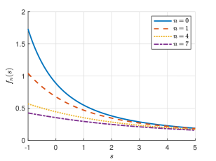
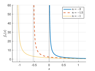
Figure A.1: Plots of the universal profile $f_{n}$

Lemma A.1 proves elementary monotonicity properties of the universal profile $f_{n}$. For its statement we define $s_{n}^{*}=\sup\{s:(n+2)f_{n+2}(s)+s=0\}$; $s_{n}^{*}=-\infty$ unless $n<0$.

Lemma A.1.

For $n\in[-2,\infty)$ and $s>s_{n}^{*}$, the universal profile $f_{n}(s)$ is strictly decreasing both as a function of $s$ and as a function of $n$.

Proof.

We first prove monotonicity in $s$. For $n=0,-2$, the functions $f_{0}(s)=I_{1}(s)$ and $f_{-2}(s)=\frac{1}{s}$ are monotone in $s$ by definition. For $k>0$, we define the probability measure $d\mu_{k,s}(x)\propto x^{k-1}e^{-\frac{1}{4}x^{4}-\frac{1}{2}sx^{2}}dx$ on $(0,\infty)$. Then for $n>0$ we have $nf_{n}(s)=\int_{0}^{\infty}x^{2}d\mu_{n,s}$, so

$$2n\frac{d}{ds}f_{n}(s)=-\int x^{4}d\mu_{n,s}+\left(\int x^{2}d\mu_{n,s}\right)^{2}.$$ (A.1)

Notice that, for any strictly increasing functions $f$ and $g$,

$$\mu_{k,s}(fg)-\mu_{k,s}(f)\mu_{k,s}(g)=\frac{1}{2}\iint d\mu_{k,s}(x)d\mu_{k,s}(y)\big{(}f(x)-f(y)\big{)}\big{(}g(x)-g(y)\big{)}>0,$$ (A.2)

(this is the FKG inequality with strict inequality) so we obtain $\frac{d}{ds}f_{n}(s)<0$. For $n\in(-2,0)$, by (1.66) it is sufficient to prove that

$$\frac{d}{ds}(n+2)f_{n+2}(s)>-1\quad\text{if}\;\;s>s_{n}^{*}.$$ (A.3)

By (A.1) and (1.62), we have

$$2(n+2)\frac{d}{ds}f_{n+2}(s) =-\frac{I_{n+5}(s)}{I_{n+1}(s)}+\Big{(}\frac{I_{n+3}(s)}{I_{n+1}(s)}\Big{)}^{2}$$

$$=-(n+2)+s(n+2)f_{n+2}(s)+\big{(}(n+2)f_{n+2}(s)\big{)}^{2}.$$ (A.4)

But since $s+(n+2)f_{n+2}(s)>0$ for $s>s_{n}^{*}$, we see that $(n+2)\frac{d}{ds}f_{n+2}(s)>-\frac{n+2}{2}>-1$.

Finally, for the monotonicity in $n$, for $k>-1$ and $q>0$ we have

$$\frac{d}{dk}\frac{I_{q+k}(s)}{I_{k}(s)} =\int x^{q}\log x\,d\mu_{k,s}-\left(\int x^{q}d\mu_{k,s}\right)\left(\int\log x\,d\mu_{k,s}\right)>0$$ (A.5)

where the final inequality follows from (A.2). (Note that this proves that the profile $\Sigma_{n,k}(s)$ in (1.33) is monotone increasing in $n>0$.) Therefore, by (1.63) and by (A.5), for all $n>-2$ we have

$$\frac{d}{dn}\frac{1}{f_{n}(s)}=\frac{d}{dn}\Big{(}\frac{I_{n+3}(s)}{I_{n+1}(s)}+s\Big{)}>0.$$ (A.6)

This proves the desired monotonicity in $n$, and the proof is complete. ∎

A cursory examination of Figure A.1 may suggest that $f_{n}$ is convex but this is misleading: Figure A.2 shows that $s\mapsto f_{1}(s)+s$ is not convex and hence neither is $f_{1}$.

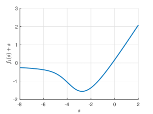
Figure A.2: Plot of $f_{1}(s)+s$ illustrating lack of convexity of $f_{1}(s)+s$ and hence of $f_{1}(s)$.

Appendix B Self-avoiding walk: proof of Propositions 1.5–1.6

In this section we prove Propositions 1.5–1.6, which we restate here as Propositions B.1–B.2.

Proposition B.1.

For self-avoiding walk on the complete graph, as $N\to\infty$,

$$\chi_{N}^{\mathbb{K}}(N^{-1}(1-s(2N)^{-1/2})) \sim(2N)^{1/2}f_{0}(s)\qquad(s\in\mathbb{R}).$$ (B.1)

Proof.

It is proved in [57, Theorem 1.1] on the basis of an exact rewriting of the susceptibility in terms of the incomplete Gamma function, that, as $N\to\infty$,

$$\chi_{N}^{\mathbb{K}}(N^{-1}(1-s(2N)^{-1/2})) \sim N^{1/2}\sqrt{\frac{\pi}{2}}e^{s^{2}/4}{\rm erfc}(s/2),$$ (B.2)

where the complementary error function is defined for $x\in\mathbb{R}$ by ${\rm erfc}(x)=\frac{2}{\sqrt{\pi}}\int_{x}^{\infty}e^{-t^{2}}dt$. With the change of variable $y=x^{2}/2$ in the definition of $I_{1}$ in (1.60), we see that

$$f_{0}(s) =I_{1}(s)=e^{\frac{1}{4}s^{2}}\int_{0}^{\infty}e^{-(y+s/2)^{2}}dy=\frac{\sqrt{\pi}}{2}e^{s^{2}/4}\operatorname{erfc}(s/2).$$ (B.3)

This proves (B.1). ∎

A detailed analysis of self-interacting walk on the complete graph is given in [10]. Although the emphasis in [10] is on elucidating the phase diagram for a model with tricritical behaviour, much of [10] applies more generally and in particular to the continuous-time weakly self-avoiding walk. The critical point $\nu_{c}=\nu_{c}(g)$ is characterised in [10, Definition 1.2] in terms of the effective potential $V:[0,\infty)\to\mathbb{R}$, defined by

$$V(t) =t-\log(1+v(t)),\qquad v(t)=\int_{0}^{\infty}e^{-gs^{2}-\nu s}e^{-s}\sqrt{\frac{t}{s}}\tilde{I}_{1}(2\sqrt{st})\,ds,$$ (B.4)

as the choice of $\nu_{c}$ for which $V_{c}^{\prime}(0)=0$, $V_{c}^{\prime\prime}(0)>0$ (the subscript $c$ denotes evaluation at $\nu_{c}$). Here $\tilde{I}_{1}$ is the modified Bessel function of the first kind (the tilde is used to avoid confusion with $I_{1}$ of (1.60)), and $V(0)=0$ since $\tilde{I}_{1}(0)=0$. See Figure B.1 for an illustration. In the following theorem, we apply the results of [10] to prove that the profile $f_{0}(s)$ arises for the susceptibility in this model in its critical window. Note that the profile is independent of the value of $g>0$, as we have also seen for $n\geq 1$ in Corollary 1.4.

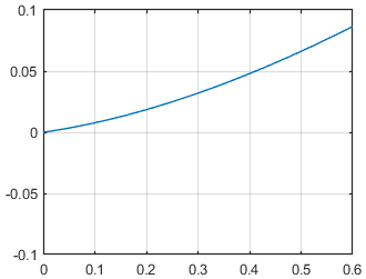
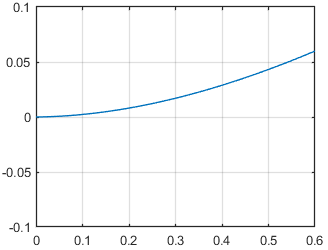
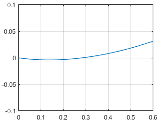
Figure B.1: Effective potential $V$ vs $t$ for $g=1$ and $\nu=-1.1,-1.2,-1.3$. The critical value is close to $-1.2$.

Proposition B.2.

There are positive constants $\lambda_{1},\lambda_{2}$ such that

$$\lim_{N\to\infty}N^{-1/2}\chi_{N}^{\rm WSAW}(\nu_{c}+sN^{-1/2}) =\lambda_{1}f_{0}(\lambda_{2}s)\qquad(s\in\mathbb{R}).$$ (B.5)

Proof.

At the critical point $\nu_{c}$, it is proved in [10, Theorem 1.3] that $G_{00}(\nu_{c})\to 1$ as $N\to\infty$, whereas $G_{01}(\nu_{c})$ is of order $N^{-1/2}$. Thus, at the critical point, $G_{00}$ does not contribute to the leading order of $\chi$, which is $\chi(\nu_{c})\sim NG_{01}$. We now extend this to the scaling window $\nu(s)=\nu_{c}+sN^{-1/2}$.

The combination of [10, (3-5))] and [10, (3-17)] gives the formula

$$G_{01}(\nu)=\int_{0}^{\infty}e^{-NV(t)}(NV^{\prime}(t)F(t,t)-\partial_{1}F(t,t))\,dt,$$ (B.6)

with $F(t_{1},t_{2})=(1-V^{\prime}(t_{1}))^{2}t_{2}$. Integration by parts then gives

$$G_{01}(\nu) =\int_{0}^{\infty}e^{-NV(t)}\Big{(}\frac{d}{dt}F(t,t)-\partial_{1}F(t,t)\Big{)}\,dt$$

$$=\int_{0}^{\infty}e^{-NV(t)}\partial_{2}F(t,t)\,dt$$

$$=\int_{0}^{\infty}e^{-NV(t)}(1-V^{\prime}(t))^{2}dt.$$ (B.7)

(This integration by parts was not done in [10]; its use would simplify some computations in [10].) We use prime and dot to denote derivatives with respect to $t$ and $\nu$, respectively. By Taylor expansion in the variable $s$, as $N\to\infty$ we have

$$V_{\nu(s)}(t) =V_{c}(t)+\dot{V}_{c}(t)sN^{-1/2}+O(s^{2}N^{-1}).$$ (B.8)

The integral on the right-hand side of (B.7) is dominated by its behaviour near $t=0$ because $V$ grows at least linearly as $t\to\infty$ by [10, Proposition 1.1], so we may restrict the integral to a finite interval and use (B.8) and [54, Ex. 4.1, p.333] to evaluate the asymptotic form of $G_{01}$ in the window. In the notation of [54, Ex. 4.1, p.333], and with (B.8), we have

$$p(t)\sim Pt^{2},\quad s(t)=St,\quad r(x,t)=O(1),\quad q(N,t)=(1-V_{c}^{\prime}(t))^{2}\sim 1,$$

$$P=\frac{1}{2}V_{c}^{\prime\prime}(0),\quad S=-\dot{V}_{c}^{\prime}(0)s,\quad\mu=2,\quad\sigma=1,\quad\lambda=1.$$ (B.9)

With $\operatorname{Fi}$ the Faxén integral (1.67), we conclude that

$$\chi_{N}^{\rm WSAW}(\nu_{c}+sN^{-1/2}) \sim NG_{01}(\nu_{c}+sN^{-1/2})\sim N\operatorname{Fi}({\textstyle\frac{1}{2},\frac{1}{2};SP^{-1/2}})\frac{1}{(PN)^{1/2}}.$$ (B.10)

According to (1.68), $\operatorname{Fi}({\textstyle\frac{1}{2},\frac{1}{2};u})=2I_{1}(-u)=2f_{0}(-u)$, and therefore we arrive at

$$\chi_{N}^{\rm WSAW}(\nu_{c}+sN^{-1/2}) \sim N^{1/2}\frac{2}{(\frac{1}{2}V_{c}^{\prime\prime}(0))^{1/2}}f_{0}\Big{(}s\frac{\dot{V}_{c}^{\prime}(0)}{(\frac{1}{2}V_{c}^{\prime\prime}(0))^{1/2}}\Big{)},$$ (B.11)

which identifies the constants $\lambda_{1},\lambda_{2}$ and completes the proof. ∎

References

- [1] M. Aizenman. Geometric analysis of fields and Ising models, Parts I and II. Commun. Math. Phys., 86:1–48, (1982).
- [2] M. Aizenman and H. Duminil-Copin. Marginal triviality of the scaling limits of critical Ising and models. Ann. Math., 194:163–235, (2021).
- [3] M. Aizenman and R. Fernández. On the critical behavior of the magnetization in high dimensional Ising models. J. Stat. Phys., 44:393–454, (1986).
- [4] M. Aizenman and R. Graham. On the renormalized coupling constant and the susceptibility in field theory and the Ising model in four dimensions. Nucl. Phys., B225 [FS9]:261–288, (1983).
- [5] R. Bauerschmidt, D.C. Brydges, and G. Slade. Scaling limits and critical behaviour of the -dimensional -component spin model. J. Stat. Phys, 157:692–742, (2014).
- [6] R. Bauerschmidt, D.C. Brydges, and G. Slade. Critical two-point function of the 4-dimensional weakly self-avoiding walk. Commun. Math. Phys., 338:169–193, (2015).
- [7] R. Bauerschmidt, D.C. Brydges, and G. Slade. Logarithmic correction for the susceptibility of the 4-dimensional weakly self-avoiding walk: a renormalisation group analysis. Commun. Math. Phys., 337:817–877, (2015).
- [8] R. Bauerschmidt, D.C. Brydges, and G. Slade. Introduction to a Renormalisation Group Method. Springer, Singapore, (2019). Lecture Notes in Mathematics Vol. 2242.
- [9] R. Bauerschmidt, J. Park, and P.-F. Rodriguez. The Discrete Gaussian model, I. Renormalisation group flow at high temperature. Preprint, https://arxiv.org/pdf/2202.02286.pdf, (2022).
- [10] R. Bauerschmidt and G. Slade. Mean-field tricritical polymers. Probab. Math. Phys, 1:167–204, (2020).
- [11] R. Bauerschmidt, G. Slade, A. Tomberg, and B.C. Wallace. Finite-order correlation length for 4-dimensional weakly self-avoiding walk and spins. Ann. Henri Poincaré, 18:375–402, (2017).
- [12] B. Berche, T. Ellis, Y. Holovatch, and R. Kenna. Phase transitions above the upper critical dimension. SciPost Phys. Lect. Notes, 136:paper 60, (2022).
- [13] P. M. Bleher and P. Major. Critical phenomena and universal exponents in statistical physics. On Dyson’s hierarchical model. Ann. Probab., 15:431–477, (1987).
- [14] P. M. Bleher and Ya. G. Sinai. Investigation of the critical point in models of the type of Dyson’s hierarchical models. Commun. Math. Phys., 33:23–42, (1973).
- [15] D.C. Brydges. Lectures on the renormalisation group. In S. Sheffield and T. Spencer, editors, Statistical Mechanics, pages 7–93. American Mathematical Society, Providence, (2009). IAS/Park City Mathematics Series, Volume 16.
- [16] D.C. Brydges and J.Z. Imbrie. End-to-end distance from the Green’s function for a hierarchical self-avoiding walk in four dimensions. Commun. Math. Phys., 239:523–547, (2003).
- [17] D.C. Brydges and J.Z. Imbrie. Green’s function for a hierarchical self-avoiding walk in four dimensions. Commun. Math. Phys., 239:549–584, (2003).
- [18] D.C. Brydges and G. Slade. A renormalisation group method. IV. Stability analysis. J. Stat. Phys, 159:530–588, (2015).
- [19] D.C. Brydges and G. Slade. A renormalisation group method. V. A single renormalisation group step. J. Stat. Phys, 159:589–667, (2015).
- [20] F. Camia, J. Jiang, and C.M. Newman. The effect of free boundary conditions on the Ising model in high dimensions. Probab. Theory Related Fields, 181:311–328, (2021).
- [21] J. Cardy. Scaling and Renormalization in Statistical Physics. Cambridge University Press, Cambridge, (1996).
- [22] J. Cardy, editor. Finite-Size Scaling. North Holland, Amsterdam, (1998). Current Physics–Sources and Comments, Vol. 2.
- [23] M. Cassandro and G. Jona-Lasinio. Critical point behaviour and probability theory. Adv. Phys., 27:913–941, (1978).
- [24] S. Chatterjee and J. Hanson. Restricted percolation critical exponents in high dimensions. Commun. Pure Appl. Math., 73:2370–2429, (2020).
- [25] S. Chatterjee and Q.-M. Shao. Nonnormal approximation by Stein’s method of exchangeable pairs with application to the Curie–Weiss model. Ann. Appl. Probab., 21:464–483, (2011).
- [26] N. Deb and S. Mukherjee. Fluctuations in mean-field Ising models. Ann. Appl. Probab., 33:1961–2003, (2023).
- [27] Y. Deng, T.M. Garoni, J. Grimm, and Z. Zhou. Unwrapped two-point functions on high-dimensional tori. J. Stat. Mech: Theory Exp., 053208, (2022).
- [28] F.J. Dyson. Existence of a phase transition in a one-dimensional Ising ferromagnet. Commun. Math. Phys., 12:91–107, (1969).
- [29] P. Eichelsbacher and M. Löwe. Stein’s method for dependent random variables occurring in statistical mechanics. Electron. J. Probab., 15:962–988, (2010).
- [30] R.S. Ellis. Entropy, Large Deviations, and Statistical Mechanics. Springer, Berlin, (1985).
- [31] R.S. Ellis and C.M. Newman. The statistics of Curie–Weiss models. J. Stat. Phys., 19:149–161, (1978).
- [32] J. Feldman, J. Magnen, V. Rivasseau, and R. Sénéor. Construction and Borel summability of infrared by a phase space expansion. Commun. Math. Phys., 109:437–480, (1987).
- [33] R. Fernández, J. Fröhlich, and A.D. Sokal. Random Walks, Critical Phenomena, and Triviality in Quantum Field Theory. Springer, Berlin, (1992).
- [34] M.E. Fisher. Scaling, universality and renormalization group theory. In F.J.W. Hahne, editor, Critical Phenomena. Springer, Berlin, (1983). Lecture Notes in Physics Vol. 186.
- [35] E. Flores-Sola, B. Berche, R. Kenna, and M. Weigel. Role of Fourier modes in finite-size scaling above the upper critical dimension. Phys. Rev. Lett., 116:115701, (2016).
- [36] J. Fröhlich. On the triviality of theories and the approach to the critical point in dimensions. Nucl. Phys., B200 [FS4]:281–296, (1982).
- [37] K. Gawȩdzki and A. Kupiainen. Triviality of and all that in a hierarchical model approximation. J. Stat. Phys., 29:683–698, (1982).
- [38] K. Gawȩdzki and A. Kupiainen. Massless lattice theory: Rigorous control of a renormalizable asymptotically free model. Commun. Math. Phys., 99:199–252, (1985).
- [39] J. Glimm and A. Jaffe. Quantum Physics, A Functional Integral Point of View. Springer, Berlin, 2nd edition, (1987).
- [40] S. Gunaratnam, C. Panagiotis, R. Panis, and F. Severo. Random tangled currents for : translation invariant Gibbs measures and continuity of the phase transition. Preprint, https://arxiv.org/pdf/2211.00319, (2022).
- [41] T. Hara, T. Hattori, and H. Watanabe. Triviality of hierarchical Ising model in four dimensions. Commun. Math. Phys., 220:13–40, (2001).
- [42] T. Hara and H. Tasaki. A rigorous control of logarithmic corrections in four dimensional spin systems. II. Critical behaviour of susceptibility and correlation length. J. Stat. Phys., 47:99–121, (1987).
- [43] T. Hutchcroft. The critical two-point function for long-range percolation on the hierarchical lattice. Preprint, https://arxiv.org/pdf/2103.17013, (2021).
- [44] T. Hutchcroft. Critical cluster volumes in hierarchical percolation. Preprint, https://arxiv.org/pdf/2211.05686, (2022).
- [45] T. Hutchcroft, E. Michta, and G. Slade. High-dimensional near-critical percolation and the torus plateau. Ann. Probab., 51:580–625, (2023).
- [46] Z. Kabluchko, M. Löwe, and K. Schubert. Fluctuations of the magnetization for Ising models on Erdős–Rényi random graphs—the regimes of small and the critical temperature. J. Phys. A: Math. Theor., 53:355004, (2020).
- [47] R. Kenna. Finite size scaling for -theory at the upper critical dimension. Nucl. Phys. B, 691 [FS]:292–304, (2004).
- [48] R. Kenna. Universal scaling relations for logarithmic-correction exponents. In Yu. Holovatch, editor, Order, Disorder, and Criticality: Advanced Problems of Phase Transition Theory, Volume 3, pages 1–46. World Scientific, Singapore, (2012).
- [49] J.L. Lebowitz. GHS and other inequalities. Commun. Math. Phys., 35:87–92, (1974).
- [50] M. Lohmann. Critical exponent for the magnetization of the weakly coupled model. Commun. Math. Phys., 376:441–486, (2020).
- [51] E. Luijten and H.W.J. Blöte. Classical critical behavior of spin models with long-range interactions. Phys. Rev. B, 56:8945–8958, (1997).
- [52] P.H. Lundow and K. Markström. The scaling window of the D Ising model with free boundary conditions. Nucl. Phys. B, 911:163–172, (2016).
- [53] E. Michta and G. Slade. Weakly self-avoiding walk on a high-dimensional torus. Probab. Math. Phys., 4:331–375, (2023).
- [54] F.W.J. Olver. Asymptotics and Special Functions. CRC Press, New York, (1997).
- [55] V. Papathanakos. Finite-Size Effects in High-Dimensional Statistical Mechanical Systems: The Ising Model with Periodic Boundary Conditions. PhD thesis, Princeton University, (2006).
- [56] B. Simon and R.B. Griffiths. The field theory as a classical Ising model. Commun. Math. Phys., 33:145–164, (1973).
- [57] G. Slade. Self-avoiding walk on the complete graph. J. Math. Soc. Japan, 72:1189–1200, (2020).
- [58] G. Slade and A. Tomberg. Critical correlation functions for the -dimensional weakly self-avoiding walk and -component model. Commun. Math. Phys., 342:675–737, (2016).
- [59] H. Watanabe. Triviality of hierarchical spin model in four dimensions with large . J. Stat. Phys., 115:1669–1713, (2004).
- [60] J.G. Wendel. Note on the Gamma function. Am. Math. Monthly, 55:563–564, (1948).
- [61] K.J. Wiese and A.A. Fedorenko. Field theories for loop-erased random walks. Nucl. Phys. B, 946:114696, (2019).
- [62] M. Wittmann and A.P. Young. Finite-size scaling above the upper critical dimension. Phys. Rev. E, 90:062137, (2014).
- [63] Z. Zhou, J. Grimm, S. Fang, Y. Deng, and T.M. Garoni. Random-length random walks and finite-size scaling in high dimensions. Phys. Rev. Lett., 121:185701, (2018).
- [64] J. Zinn-Justin. Quantum Field Theory and Critical Phenomena. Oxford University Press, Oxford, 5th edition, (2021).