Optimal Sampling-based Motion Planning in Gaussian Belief Space for Minimum Sensing Navigation

Abstract

In this paper, we consider the motion planning problem in Gaussian belief space for minimum sensing navigation. Despite the extensive use of sampling-based algorithms and their rigorous analysis in the deterministic setting, there has been little formal analysis of the quality of their solutions returned by sampling algorithms in Gaussian belief space. This paper aims to address this lack of research by examining the asymptotic behavior of the cost of solutions obtained from Gaussian belief space based sampling algorithms as the number of samples increases. To that end, we propose a sampling based motion planning algorithm termed Information Geometric PRM* (IG-PRM*) for generating feasible paths that minimize a weighted sum of the Euclidean and an information-theoretic cost and show that the cost of the solution that is returned is guaranteed to approach the global optimum in the limit of large number of samples. Finally, we consider an obstacle-free scenario and compute the optimal solution using the ”move and sense” strategy in literature. We then verify that the cost returned by our proposed algorithm converges to this optimal solution as the number of samples increases.

1 Introduction

Over the past few decades, motion planning has been an active area of research in the robotics community. Motion planning can be broadly classified into three main categories, mainly grid based Ding et al. (2019a); MacAllister et al. (2013), optimization based Mercy et al. (2017); Kushleyev et al. (2013); Deits and Tedrake (2015) and sampling based algorithms Karaman and Frazzoli (2011). Sampling-based planning algorithms sample points in the configuration space and check whether a connection is possible between the sampled points using collision-checking modules which are treated as a black box and are usually computationally expensive. They have shown success in handling high dimensional motion planning problems for instance manipulators Khan et al. (2020), warehouse robots, aerial robotics Lee et al. (2016) etc. In the field of robotic motion planning, it is common to first generate a reference path (usually using sampling based algorithms Karaman and Frazzoli (2011); Hart et al. (1968); Kavraki et al. (1996); LaValle and Kuffner (2001); Janson et al. (2015); Zinage and Ghosh (2020)) and then separately design a feedback control system for following that path. While this two-step approach is not optimal in general, it simplifies the overall problem and is acceptable in many cases. Additionally, this two-step method can take advantage of powerful geometry-based trajectory generation algorithms (such as Gao and Shen (2016); Liu et al. (2017); Mellinger and Kumar (2011); Ding et al. (2019b); Zinage et al. (2023)), which allows for addressing other considerations such as dynamic constraints, randomness, and uncertainty during the control design phase. Despite these benefits, it is important to acknowledge the inherent challenges posed by measurement noise and uncertainty in robotics.

In light of these fundamental and inevitable issues, a different perspective may be more advantageous when planning under uncertainty. Instead of using deterministic boolean indicators to check for collisions in feasible paths, as is done in planning without uncertainty, it is preferable to represent the state of the agent as a probability distribution over the states in the configuration space. These states are known as the belief state or the information state. Planning under uncertainty can be formulated as a Partially Observable Markov Decision Process (POMDP) Astrom (1965); Smallwood and Sondik (1973); Kaelbling et al. (1998). In general, for real-world problems, it becomes computationally intractable to compute the solution of these POMDPs despite the recent progress to solve these POMDPs. Planning in belief spaces that are infinite-dimensional becomes more tractable from a generated roadmap using sampling based motion planning algorithms. Therefore, sampling-based algorithms are considered more advantageous for these infinite-dimensional motion planning problems.

The main motivation for this paper arises from the need for simultaneous perception and planning in autonomous systems to address the problem of finding the shortest path while minimizing sensory resource consumption. Advanced and affordable sensing devices have made it easier to gather sensor data, but this may not always be efficient for resource-limited robots due to the significant power and computational resources required. As the number of sensor modalities increases, it is crucial to minimize the use of sensory resources while ensuring that the algorithm converges to an optimal solution rather than a suboptimal one, as the latter can lead to higher costs. In this paper, we propose the Information Geometric PRM* (IG-PRM*), a sampling-based planning algorithm for minimum sensing navigation that computes a reference path in Gaussian belief space, minimizing the weighted sum of Euclidean and perception costs, with the latter being a quasi-pseudo metric. Our main contribution is the proof of asymptotic optimality for IG-PRM*. The asymptotic optimality of a related algorithm termed IG-RRT* was already conjectured in Pedram et al. (2022). Asymptotic optimality is essential in motion planning, as it guarantees that the algorithm will eventually find a solution as close as desired to the optimal one, without getting stuck in a suboptimal solution. Following Pedram et al. (2021, 2022), our goal is to develop an asymptotic optimal path planning methodology that enables a robot to navigate using the minimum amount of sensing resources while adapting to any constraints on its sensory resources.

2 Related work

2.1 Belief space motion planning

In the continuous state, control, and observation space, the complexity of the POMDP framework makes it difficult to use. Towards the aim of addressing this issue, the area of belief space path planning computes feasible paths for uncertain systems that take into account the uncertainty in the system’s dynamics and environment. Censi et al. (2008) proposed a planning algorithm that uses graph search and constraint propagation on a grid-based representation of the space. Platt Jr et al. (2010) used nonlinear optimization methods to find the best nominal path in continuous space. The linear quadratic Gaussian motion planning (LQGMP) method Van Den Berg et al. (2011) computes the best possible feasible path among a finite number of paths generated by RRT by simulating the performance of an LQG controller on all of them. Bry and Roy (2011) utilized a tree-based approach to optimize the underlying nominal trajectory using RRT*. Vitus and Tomlin (2011) also addressed the optimization of the underlying trajectory by formulating it as a chance-constrained optimal control problem. Prentice and Roy (2009) also used roadmap-based methods based on the Probabilistic Roadmap (PRM) approach, where the optimal path is found through a breadth-first search on the belief roadmap (BRM). However, in all of these roadmap-based methods, the optimal substructure assumption is violated, meaning that the costs of different edges on the graph depend on one another. In Kurniawati et al. (2012), the point-based POMDP (Partially Observable Markov Decision Process) planner takes into account uncertainties in motion, observation, and mapping, and improves upon previous point-based methods through the use of guided cluster sampling. This method starts with a roadmap in the configuration space and grows a single-query tree in the belief space, rooted in the initial belief. Roy et al. (1999) examines the use of a coastal navigation strategy to assist the agent’s perception during navigation.

2.2 Chance constrained motion planning

Chance constrained motion planning is a class of planning algorithms that take into consideration probabilistic safety constraints. This approach is closely related to the field of belief space path planning, which involves finding paths that meet specific safety requirements under uncertainty Blackmore et al. (2006, 2011); Vitus and Tomlin (2011). There have been efforts to extend basic chance-constrained methods, which are primarily designed for linear-Gaussian systems, to handle more complex, non-linear, and non-Gaussian problems, as well as to address joint chance constraints Blackmore et al. (2010); Wang et al. (2020); Ono et al. (2015). However, these formulations can be computationally expensive and may not scale well. To address this issue, several methods were proposed to improve scalability, while others have developed sampling-based approaches like CC-RRT (chance-constrained rapidly-exploring random tree) that allow for efficient computation of feasible paths. The CC-RRT algorithm has been generalized for use in dynamic environments, and several variants have been introduced that guarantee convergence to the optimal trajectory. Tree-based planners with chance constraints have been shown to be efficient and have been used in unknown environments through iterative planning in several studies Luders et al. (2010); Pairet et al. (2021); Plaku et al. (2010). Some studies have also extended these frameworks to systems with measurement uncertainty, using maximum-likelihood observations to approximate solutions Platt Jr et al. (2010), although this approach does not provide safety guarantees.

2.3 Information theoretic path planning

In an objective function of belief space path planning, an information-theoretic cost is a measure of uncertainty in the system, which is usually quantified using mutual information. For Gaussian distributions, calculation of the cost usually involves computing the determinant of a posteriori covariance matrix, which has a complexity of $O(n^{3})$ in general cases, where $n$ is the state dimension. This computation needs to be performed for each potential action. In Indelman et al. (2015), a method was proposed to address this challenge by using information form and exploiting sparsity, but this still requires expensive access to marginal probability distributions. The rAMDL approach Kopitkov and Indelman (2017) performs a one-time calculation of the marginal covariances of the variables involved in the candidate actions, and then uses an augmented matrix determinant lemma (AMDL) to efficiently evaluate the information-theoretic cost for each action. However, this method still requires the recovery of appropriate marginal covariances, the complexity of which depends on the state dimensionality and the sparsity of the system. Levine et al. (2013) focused on finding ways for sensing agents to both gather as much information as possible about their target or environment, as measured by the Fisher information matrix, and minimize the cost of reaching their goal. In Folsom et al. (2021), a Mars helicopter used an RRT*-IT algorithm to explore the surface of Mars and reduce uncertainty about the terrain type in the shortest amount of time.

2.4 Technical contributions

The technical contributions of this paper are as follows.

1. We consider the shortest path problem for minimum sensing navigation in Gaussian belief space with respect to a cost function that represents the weighted sum of the Euclidean and the information-theoretic sensing cost and propose a sampling-based motion planning algorithm termed Information Geometric PRM* (IG-PRM*) algorithm.

2. We prove that the IG-PRM* algorithm is asymptotically optimal. One of the main challenges in establishing asymptotic optimality in Gaussian belief space as compared to deterministic space is the characterization of the volume of covariances and the computation of the associated probability of sampling these covariance matrices. To address this challenge, our second contribution is based on the following two novel results. First, we provide an analytical expression for computing the volume of covariance matrices in the space of symmetric matrices equipped with Rao-Fisher metric and derive a lower bound for this volume in terms of the Selberg integral. Second, we provide a lower bound for the probability of sampling these covariance matrices. These two results aid in establishing the asymptotic optimality of IG-PRM*. To the best knowledge of the authors, this is the first paper that addresses the problem of asymptotic optimality in Gaussian belief space.

3. Through numerical simulations, we verify our claim that the cost returned by IG-PRM* in the absence of any obstacle converges to the optimal cost in the limit of large number of samples. The optimal cost can be analytically computed using the move and sense strategy in the literature Pedram et al. (2022).

2.5 Outline of the paper

The paper is organized as follows. Section 2.6 discusses the nomenclature followed by preliminaries in Section 3. Section 4 discusses the problem statement we address in the paper followed by the proposed algorithm and main result in Sections 5 and 6 respectively. In Section 7, we extend the proposed algorithm. Finally, Section 8 discusses the numerical simulations and verify the claims made in the paper followed by some concluding remarks in Section 9.

2.6 Notation and convention

Matrices and vectors are represented by uppercase and lowercase letter respectively. The following notation will be used. $\mathbb{S}^{d}=\left\{P\in\mathbb{R}^{d\times d}:P\text{ is symmetric.}\right\}$, $\mathbb{S}_{+}^{d}=\left\{P\in\mathbb{R}^{d\times d}:P\succ 0\right\}$ and $\mathbb{S}_{\rho}^{d}=\left\{P\in\mathbb{S}^{d}:P\succeq\rho I,\;\rho>0\right\}$. $\mathcal{E}_{\chi^{2}}(x_{0},P_{0})=\{x\in\mathbb{R}^{d}:(x-x_{0})^{\top}P_{0}^{-1}(x-x_{0})<\chi^{2}\}$ is the confidence ellipse. Throughout this paper, we assume that the value of $\chi^{2}$ is fixed. $\mathcal{B}(x_{0},r_{0})=\{x\in\mathbb{R}^{d}:(x-x_{0})^{\mathrm{T}}(x-x_{0})\leq r_{0}\}$ is the ball with center at $x_{0}$ and radius $r_{0}$. $\lambda_{i}(X)$ for all $i\in\{1,2,\dots,d\}$ denote the eigenvalues of a positive definite matrix $X$ and without loss of generality, we assume that $\lambda_{1}\leq\lambda_{2}\dots\leq\lambda_{d}$. For integers $a$ and $b(\geq a)$, $[a;b]$ denotes the set $\{a,a+1,\dots,b\}$. $\mathcal{N}(x,P)$ represents a Gaussian random variable with mean $x$ and covariance $P$. $\bar{\sigma}(M)$ denotes the maximum singular value of $M$. The Euclidean and the Frobenius norm are represented by $\|.\|$ and $\|.\|_{F}$, respectively.

3 Preliminaries

This section provides a brief overview of our setup, which closely mirrors that of Pedram et al. (2022). We include this information for the sake of completeness.

3.1 Dynamic model

Consider a sequence of way points $\{x_{k}\}_{k\in[1;K]}$ in the configuration space $\mathbb{R}^{d}$. Let $t_{k}$ be the time that the agent is scheduled to visit the $k^{\text{th}}$ way point $x_{k}$. The agent is assumed to apply a constant velocity input

$$v(t)=v_{k}:=\frac{x_{k+1}-x_{k}}{t_{k+1}-t_{k}}$$

for $t_{k}\leq t<t_{k+1},k\in[1;K-1]$. We assume that the agent motion is subject to stochastic disturbance. Let ${\bf x}(t_{k})$ be the random vector representing the robot’s actual position at time $t_{k}$. It is assumed to satisfy

$${\bf x}(t_{k+1})={\bf x}(t_{k})+(t_{k+1}-t_{k})v_{k}+{\bf n}_{k}$$ (1)

where ${\bf n}_{k}\sim\mathcal{N}(0,\|x_{k+1}-x_{k}\|W)$. Note that the constant velocity input and dynamics (1) are assumed exclusively for the purpose of establishing a distance concept within a Gaussian belief space as presented in subsequent sections. Despite potential significant differences between actual robot dynamics and (1), the algorithm we propose in Section 4 remains applicable. This approach is analogous to the widespread use of RRT* (or other sampling based motion planning algorithms) for Euclidean distance minimization in scenarios where Euclidean distance in configuration space fails to accurately represent motion costs. In line with this reasoning, we deliberately adopt a simplistic model (1) and reserve addressing more accurate dynamic constraints for the path-following control phase.

3.2 Gaussian belief space

Let the probability distributions of the robot position at time step $k$ can be characterized by a Gaussian model as ${\bf x}_{k}\sim\mathcal{N}(x_{k},P_{k})$, where $x_{k}\in\mathbb{R}^{d}$ is the mean position and $P_{k}\in\mathbb{S}_{+}^{d}$ is the covariance matrix. We first introduce an appropriate directed distance function from a point $(x_{k},P_{k})\in\mathbb{R}^{d}\times\mathbb{S}_{+}^{d}$ to another $(x_{k+1},P_{k+1})\in\mathbb{R}^{d}\times\mathbb{S}_{+}^{d}$. The distance function is interpreted as the cost of steering the state random variable ${\bf x}_{k}\sim\mathcal{N}(x_{k},P_{k})$ at time $k$ to ${\bf x}_{k+1}\sim\mathcal{N}(x_{k+1},P_{k+1})$ in the next time step under the dynamics (1). We assume that the distance function is a weighted sum of the travel cost $\mathcal{D}_{\text{travel}}(k)$ and the information cost $\mathcal{D}_{\text{info}}(k)$.

3.2.1 Travel cost:

We assume that the travel cost is simply the commanded travel distance:

$$\mathcal{D}_{\text{travel}}(k):=\|x_{k+1}-x_{k}\|$$

3.2.2 Information cost:

We define the information-theoretic cost function $\mathcal{D}_{\text{info}}(k)$ at time step $k$ as follows:

$$\mathcal{D}_{\text{info}}(k)=\!\!\min_{Q_{k+1}\succeq 0}\!\! \quad\frac{1}{2}\log\det\hat{P}_{k+1}-\frac{1}{2}\log\det Q_{k+1}$$ (2a)

s.t. $$\quad Q_{k+1}\preceq P_{k+1},\;\;Q_{k+1}\preceq\hat{P}_{k+1}.$$ (2b)

Notice that for any given pair of the origin $(x_{k},P_{k})$ and the destination $(x_{k+1},P_{k+1})$, (2a) takes a nonnegative value. For more details and motivation for using this cost function, we suggest the readers refer to Pedram et al. (2022).

3.2.3 Total cost:

The total cost to steer the state random variable ${\bf x}_{k}\sim\mathcal{N}(x_{k},P_{k})$ to ${\bf x}_{k+1}\sim\mathcal{N}(x_{k+1},P_{k+1})$ is a weighted sum of $\mathcal{D}_{\text{travel}}(k)$ and $\mathcal{D}_{\text{info}}(k)$ as

$$\mathcal{D}(x_{k},x_{k+1},P_{k},P_{k+1}):=\;\mathcal{D}_{\text{travel}}(k)+\alpha\mathcal{D}_{\text{info}}(k),$$ (3)

where $\alpha\geq 0$ is the weight factor.

3.3 Chains and Paths

Suppose that a sequence $\{(x_{k},P_{k})\}_{k\in[1;K-1]}$ is given. In what follows, the sequence of transitions from $(x_{k},P_{k})$ to $(x_{k+1},P_{k+1})$, ${k\in[1;K-1]}$ will be referred to as a chain. Notice that the parameter $t$ does not necessarily correspond to the physical time. The time of arrival of the agent at the end point depends on the length of the path and the travel speed of the robot.

3.3.1 Lossless Chains and Paths:

A transition from $(x_{k},P_{k})$ to $(x_{k+1},P_{k+1})$ is said to be lossless if

$$P_{k+1}\preceq\hat{P}_{k+1}(:=P_{k}+\|x_{k+1}-x_{k}\|W)$$ (4)

If every transition in the sequence $\{(x_{k},P_{k})\}_{k\in[1;K]}$ is lossless, we say that the sequence is lossless. Let $\gamma:[0,T]\rightarrow\mathbb{R}^{d}\times\mathbb{S}_{+}^{d}$, $\gamma(t)=(x(t),P(t))$ be a path. In what follows, the variable $t$ is called the time parameter. The travel length of the path $\gamma$ from time $t=t_{a}$ to time $t=t_{b}$ is defined as

$$\ell(\gamma_{x}[t_{a},t_{b}])=\sup_{\mathcal{P}}\sum_{k=1}^{K}\|x(t_{k})-x_{k+1}\|$$

where the supremum is over the space of all partitions $\mathcal{P}=(t_{a}=t_{0}<t_{1}<\cdots<t_{K}=t_{b})$. We say that a path $\gamma$ is lossless if the condition

$$P(t_{b})\preceq P(t_{a})+\ell(\gamma_{x}[t_{a},t_{b}])W$$ (5)

for any $0\leq t_{a}<t_{b}\leq T$. Notice that the right hand side of (5) is the covariance of the position of the robot which had the initial configuration $(x(t_{a}),P(t_{a})$ and traveled along the path $\gamma_{x}[t_{a},t_{b}]$ under the dynamics (1) without sensing. Therefore, the inequality (5) means that the growth of uncertainty from $P(t_{a})$ to $P(t_{b})$ is never greater that the ”natural growth” $\ell W$, which is always true in realistic navigation scenarios. A path $\gamma$ is said to be finitely lossless if there exists a finite $N$ and a partition $\mathcal{P}=(0=t_{0}<t_{1}<\cdots<t_{K}=T)$ such that for each $k\in[1;K]$, the transition from $(x(t_{k}),P(t_{k}))$ to $(x^{\prime}(t_{k}),P^{\prime}(t_{k}))$ is lossless

Remark 1.

If a path $\gamma$ is finitely lossless with respect to a partition $\mathcal{P}$, then it is also finitely lossless with respect to a partition $\mathcal{P}^{\prime}$, provided $\mathcal{P}^{\prime}\supseteq\mathcal{P}$ (i.e., $\mathcal{P}^{\prime}$ is a refinement of $\mathcal{P}$). Based on this observation, it can be shown that if a path is finitely lossless then it is lossless. However, the converse is not always true.

3.3.2 Collision-free Chains and Paths:

Let $\mathcal{X}_{\text{obs}}\subset\mathbb{R}^{d}$ be a closed subset representing obstacles. Consider a transition from $x_{k}$ to $x_{k+1}$. The robot’s mean position during this transition is parameterized as

$$x(\lambda)=(1-\lambda)x_{k}+\lambda x_{k+1}\;\;\forall\;\;\lambda\in[0,1].$$

Assuming that the initial covariance is $P_{k}$, the evolution of the covariance matrix is written as

$$P(\lambda)=P_{k}+\lambda\|x_{k+1}-x_{k}\|W\;\;\forall\;\;\lambda\in[0,1].$$

For a fixed confidence level parameter $\chi^{2}>0$, we say that the transition from $(x(0),P(0))$ to $(x(1),P(1))$ is collision-free if

$$(x(\lambda)-x_{\text{obs}})^{\top}P(\lambda)^{-1}(x(\lambda)-x_{\text{obs}})\geq\chi^{2},$$

$$\quad\quad\quad\forall\;\lambda\in[0,1],\quad\forall x_{\text{obs}}\in\mathcal{X}_{\text{obs}}.$$

Remark 2.

A collision is detected when

$$(x(\lambda)-x_{\text{obs}})^{\top}P(\lambda)^{-1}(x(\lambda)-x_{\text{obs}})<\chi^{2}\quad$$

for all $\lambda\in[0,1]$ and $x_{\text{obs}}\in\mathcal{X}_{\text{obs}}$. The process of detecting collisions can be thought of as a problem of determining whether a particular set of conditions is feasible which is a convex program for each convex obstacle $\mathcal{X}_{\text{obs}}$ Pedram et al. (2022).

$$\begin{bmatrix}\chi^{2}&(1\!-\!\lambda)x_{k}^{\top}\!+\!\lambda x_{k+1}^{\top}\!-\!x_{\text{obs}}^{\top}\\ (1\!-\!\lambda)x_{k}\!+\!\lambda x_{k+1}\!-\!x_{\text{obs}}&P_{k}+\lambda\|x_{k+1}-x_{k}\|W\end{bmatrix}\succ 0,$$

$$\quad\quad\quad\quad\quad 0\leq\lambda\leq 1,\quad x_{\text{obs}}\in\mathcal{X}_{\text{obs}}$$ (6)

We say that a chain $\{(x_{k},P_{k})\}_{k\in[1;K]}$ is collision-free if for each $k\in[1;K-1]$, the transition from $x_{k}$ to $x_{k+1}$ with the initial covariance $P_{k}$ is collision-free. We say that a path $\gamma:[0,1]\rightarrow\mathbb{R}^{d}\times\mathbb{S}_{+}^{d}$, $\gamma(t)=(x(t),P(t))$ is collision-free if

$$(x(t)-x_{\text{obs}})^{\top}P^{-1}(t)(x(t)-x_{\text{obs}})\geq\chi^{2},$$

$$\quad\quad\quad\forall\;t\in[0,1],\quad\forall\;x_{\text{obs}}\in\mathcal{X}_{\text{obs}}.$$ (7)

4 Problem Formulation

4.1 Path length

Let $\gamma:[0,1]\rightarrow\mathbb{R}^{d}\times\mathbb{S}_{+}^{d}$, $\gamma(t)=(x(t),P(t))$ be a path, and $\mathcal{P}=(0=t_{0}<t_{1}<\cdots<t_{K_{n}}=1)$ be a partition. The length of the path $\gamma$ with respect to the partition $\mathcal{P}$ is defined as

$$c(\gamma;\mathcal{P})=\sum_{k=1}^{K_{n}-1}\mathcal{D}(x(t_{k}),x(t_{k+1}),P(t_{k}),P(t_{k+1}))$$ (8)

The length of a path $\gamma$ is defined as the supremum of $c(\gamma;\mathcal{P})$ over all partitions

$$c(\gamma):=\sup_{\mathcal{P}}c(\gamma;\mathcal{P}).$$ (9)

The definition (9) states that for any path with a finite length, there exists a sequence of partitions $\{\mathcal{P}_{i}\}_{i\in\mathbb{N}}$ such that $\underset{n\rightarrow\infty}{\lim}\;c(\gamma;\mathcal{P}_{i})=c(\gamma)$.

4.2 Topology on the path space

The space of generalized paths is a vector space on which addition and scalar multiplication are defined as $\left(\gamma_{1}+\gamma_{2}\right)(t)=\left(x_{1}(t)+x_{2}(t),P_{1}(t)+P_{2}(t)\right)$ and $a\gamma(t)=(ax(t),aP(t))$ for $a\in\mathbb{R}$, respectively. Let $\mathcal{P}=\left(0=t_{0}<t_{1}<\cdots<t_{K}=T\right)$ be a partition. The total variation of a generalized path $\gamma$ with respect to $\mathcal{P}$ is defined as $|\gamma|_{\mathrm{TV}}=\underset{{\mathcal{P}}}{\sup}\;\|x(0)\|\bar{\sigma}(W)+\bar{\sigma}(P(0))+\sum_{k=0}^{K-1}\left[\|x\left(t_{k+1}\right)-\right.$ $\left.x\left(t_{k}\right)\|\bar{\sigma}(W)+\bar{\sigma}\left(P\left(t_{k+1}\right)-P\left(t_{k}\right)\right)\right]$.

4.3 Problem statement

Given an initial belief state $b_{0}=\left(x_{0},P_{0}\right)\in\mathbb{B}$ be a given initial belief state, a closed subset $\mathcal{B}_{\text{target }}\subset$ $\mathbb{B}$ representing the desired target belief region, and $X_{\text{obs }}^{m}\subset\mathbb{R}^{d}$ be the given obstacle $m\in\{1,\ldots,M\}$ where $M\in\mathbb{N}$. Given a confidence level parameter $\chi^{2}>0$, the problem is to find the shortest path, and can be formulated as

$$\begin{array}[]{cl}&\underset{{\gamma\in\mathcal{B}\mathcal{V}[0,T]}}{\min}\;\;c(\gamma)\\ &\text{ s.t. }\gamma(0)=b_{0},\;\;\;\gamma(T)\in\mathcal{B}_{\text{target }}\\ &\left(x(t)-x_{\text{obs }}\right)^{\top}P^{-1}(t)\left(x(t)-x_{\text{obs }}\right)\geq\chi^{2}\\ &\forall t\in[0,T],\quad\forall x_{\text{obs }}\in X_{\text{obs }}^{m},\quad\forall\;m\in\{1,\ldots,M\}.\end{array}$$ (14)

In addition, the proposed algorithm must guarantee that the generated feasible chain converges to the global optimal cost $c^{\star}$ as the number of samples tends to infinity (Section 4.5 ).

Assumption 1.

We assume there exists a feasible path $\gamma(t)=(x(t),P(t))$ for the formulated problem (14) such that $P(t)\in\mathbb{S}^{d}_{4\rho}$ and $\textup{Tr}(P(t))\leq R$  for all $t\in[0,1]$ and $R>0$.

4.4 Continuity of path cost

Theorem 1.

Let $\gamma:[0,1]\rightarrow\mathbb{R}^{d}\times\mathbb{S}_{\rho}^{d}$ and $\gamma^{\prime}:[0,1]\rightarrow\mathbb{R}^{d}\times\mathbb{S}_{\rho}^{d}$ be paths. Suppose $\gamma\in\mathcal{BV}[0,1]$ and $\gamma^{\prime}\in\mathcal{BV}[0,1]$ and they are both finitely lossless. Then, for each $\epsilon>0$, there exists $\delta>0$ such that

$$|\gamma^{\prime}-\gamma|_{\text{TV}}\leq\delta\quad\Rightarrow\quad|c(\gamma^{\prime})-c(\gamma)|\leq\epsilon.$$

Proof.

Please see (Pedram et al., 2022, Appendix D) ■

4.5 Asymptotic optimality

Let $Y_{n}$ denote the cost of the least cost solution returned by a sampling-based motion planning algorithm in $n$ iterations. We define $c^{\star}=\inf\{c(\gamma):\;\gamma\;\text{is a feasible path}\}$. An algorithm is said to be asymptotically optimal if

$$P(\{\underset{n\rightarrow\infty}{\limsup}\;Y_{n}=c^{\star}\})=1$$ (15)

5 IG-PRM* Algorithm

In section, we first present the notion of uniformly sampling covariances followed by the IG-PRM* algorithm.

5.1 Uniform sampling of covariance

To introduce a sampling-based planning algorithm in a Gaussian belief space, we will need a mechanism that allows us to randomly generate candidate covariance matrices. We use the algorithm proposed in Mittelbach et al. (2012) for uniformly sampling covariance $P\in\mathbb{S}^{d}_{+}$ in $\mathcal{R}_{(\underline{c},\bar{c}]}:=\{P\in\mathbb{S}^{d}_{+}:\underline{c}<\textup{Tr}(P)\leq\bar{c}\}$. The sampled covariance $P$ is said to have uniform distribution on $\mathcal{R}_{[\underline{c},\bar{c}]}$ if

$$\mathbb{P}(\{P\in\mathcal{A}\})=\frac{\text{vol}(\mathcal{A}\cap\mathcal{R}_{[\underline{c},\bar{c}]})}{\text{vol}(\mathcal{R}_{[\underline{c},\bar{c}]})}$$ (16)

holds for all $\mathcal{A}\subset\mathbb{S}^{d}_{+}$. We denote by set $\mathcal{R}:=\{P\in\mathbb{S}^{d}_{+}:\textup{Tr}(P)=1\}$. We assume the space of $\mathbb{S}^{d}_{+}$ is equipped with the Rao-Fisher metric Terras (2012), and use this metric to measure the volume of different regions in $\mathcal{S}^{d}_{+}$ in the following Theorem.

Theorem 2.

Mittelbach et al. (2012) The volume of region $\mathcal{R}_{(c_{1},c_{2}]}$ where $c_{2}>c_{1}$ is given by

$$\textup{Vol}(\mathcal{R}_{(c_{1},c_{2}]})$$

$$=\left(\frac{c_{2}^{\frac{d(d+1)}{2}}-c_{1}^{\frac{d(d+1)}{2}}}{\frac{d(d+1)}{2}}\right)V_{r}$$

$$=\left(\frac{c_{2}^{\frac{d(d+1)}{2}}-c_{1}^{\frac{d(d+1)}{2}}}{\frac{d(d+1)}{2}}\right)\pi^{\frac{1}{4}d(d-1)}\frac{\prod_{k=2}^{d}\Gamma\left(\frac{k+1}{2}\right)}{\Gamma\left(\frac{d(d+1)}{2}\right)}$$ (17)

where $V_{r}=\textup{Vol}(\mathcal{R})$ and $\Gamma$ is the gamma function.

Proof.

Please refer to Mittelbach et al. (2012). ■

Theorem 3.

The volume of region $\mathcal{D}_{A}=\{Q\in\mathbb{S}^{d}_{+}:Q\preceq A:=\textup{diagonal}(a_{1},\dots,a_{d})\}$ is lower bounded as

$$\textup{Vol}(\mathcal{D}_{A})\geq V_{d}b^{\frac{d(d+1)}{2}}S_{d}(1,1,1/2)=\textup{Vol}(\mathcal{D}^{\prime}_{A})$$ (18)

where $b=\underset{k\in[1;d]}{\min}\;a_{k}$, $\mathcal{D}^{\prime}_{A}=\{P\in\mathbb{S}^{d}_{+}:\;P\preceq bI\}$, $V_{d}=(d!\;2^{d})^{-1}\frac{2^{d}\pi^{d^{2}/2}}{\Gamma_{d}(d/2)}$ and $S_{d}(\alpha_{1},\alpha_{2},\alpha_{3})$ is the Selberg integral given by

$$S_{d}(\alpha_{1},\alpha_{2},\alpha_{3})$$

$$=\int_{0}^{1}..\int_{0}^{1}\prod_{i=1}^{d}t_{i}^{\alpha_{1}-1}\left(1-t_{i}\right)^{\alpha_{2}-1}\prod_{1\leq i<j\leq d}\left|t_{i}-t_{j}\right|^{2\alpha_{3}}dt$$

$$=\prod_{j=0}^{d-1}\frac{\Gamma(\alpha_{1}+j\alpha_{3})\Gamma(\alpha_{2}+j\gamma)\Gamma(1+(j+1)\gamma)}{\Gamma(\alpha_{1}+\alpha_{2}+(d+j-1)\alpha_{3})\Gamma(1+\alpha_{3})}$$

Further, for $\beta>1$, we have

$$\textup{Vol}(\mathcal{D}_{\beta A})-\textup{Vol}(\mathcal{D}_{A})$$

$$\geq V_{d}(\beta^{\frac{d(d+1)}{2}}-1)b^{\frac{d(d+1)}{2}}S_{d}(1,1,1/2)$$ (19)

where $\Gamma$ is the gamma function.

Proof.

Please, see Appendix A. ■

Lemma 1.

If $P\in\mathbb{S}^{d}_{+}$ has the eigenvalue decomposition $P=V^{\top}\Sigma V$, where $\Sigma$ is diagonal and $V$ is a unitary matrix, then

$$\textup{Vol}(\mathcal{D}_{P})=\textup{Vol}(\mathcal{D}_{\Sigma}),$$ (20)

where $\mathcal{D}_{P}=\{Q\in\mathbb{S}^{d}_{+}:Q\preceq P\}$ and $\mathcal{D}_{\Sigma}=\{Q\in\mathbb{S}^{d}_{+}:Q\preceq\Sigma\}$.

Proof.

Please, see Appendix B ■

The pseudo code for generating positive definite matrices uniformly from $\mathcal{R}_{(\underline{c},\bar{c}]}$ is described in Algorithms 1-4 of Mittelbach et al. (2012).

5.2 IG-PRM* Algorithm

The implementation of PRM* in Gaussian belief space (termed as IG-PRM*) for the introduced cost function (3) is summarized in Algorithm 1. The source code for Algorithm 1 is available at https://github.com/AlirezaPedram/RI-PRMstar. PRM* Karaman and Frazzoli (2010) creates a probabilistic roadmap in deterministic configuration space by connecting randomly sampled points, and efficiently finds the shortest path between two points while maintaining asymptotic optimality. At the first glance, Algorithm 1 seems identical to the original PRM*. However, the implementation in Gaussian belief space necessitates the introduction of new functionalities.

1 Inputs: $b_{\text{init}},\;b_{\text{final}},\;n$ ;

2 $\left.B\leftarrow\left\{b_{\text{init}}\right\}\cup\{\text{SampleFree}_{i}\right\}_{i\in[1;n]}\cup\left\{b_{\text{final}}\right\}$;

3 $E\leftarrow\emptyset$;

4 for $b\in B$ do

5       $\;\;B_{\text{nbors}}\leftarrow\operatorname{Near}\left(B,b,D_{\text{min}}\right)$;

6       for $b_{j}\in B_{\text{nbors}}$ do

7             if $\operatorname{CollisionFree}(b,b_{j},\chi^{2})$  then

8                  $E\leftarrow E\cup\{(b,b_{j})\}$;

9                  

10            

11      

12$G=(B,E)$;

13 $\gamma_{n}\leftarrow\;\text{Search}(G,b_{\text{init}},b_{\text{final}},k)$;

return $\gamma_{n}$

Algorithm 1 IG-PRM*

1 Inputs: $G,b_{\text{init}},b_{\text{final}},k$ ;

2 $N_{b_{\text{init}}}\leftarrow\text{Near}_{\text{from}}(G,b_{\text{init}},k)$;

3 $N_{b_{\text{final}}}\leftarrow\text{Near}_{\text{to}}(G,b_{\text{final}},k)$;

4 $\gamma_{n}\leftarrow\text{ShortestPath}(G,N_{b_{\text{init}}},N_{b_{\text{final}}})$;

return $\gamma_{n}$

Algorithm 2 Search Algorithm (Search($G,b_{\text{init}},b_{\text{final}},k$))

1 Inputs: $\gamma_{n}:=(b_{1}\rightarrow b_{1}\dots\rightarrow b_{m})$ ;

2 for $j=2$ to $m$ do

3       $b_{j}\leftarrow\text{LosslessRefine}(b_{j-1},b_{j})$;

4      

5

return $\gamma_{n}$

Algorithm 3 Lossless modification of $\gamma_{n}$

The IG-PRM* (Algorithm 1) takes in as inputs, the initial belief state $b_{\text{init}}$, the final belief state $b_{\text{final}}$ and the total number of belief states $n$ that would be sampled. The function $\textup{SampleFree}_{i}$ (Line 2 of Algorithm 1) generates a belief state $b_{i}=(x_{i},P_{i})$ by sampling the mean state $x_{i}$ and the corresponding covariance $P_{i}$ independently. The point $x_{i}$ is sampled uniformly from obstacle free space $\mathcal{X}_{\text{free}}\in\mathbb{R}^{d}$ and $P_{i}$ is sampled uniformly from $\mathcal{R}_{(\rho d,R]}:=\{P\in\mathbb{S}^{d}_{+}:\;\rho d<\textup{Tr}(P)\leq R\}$ by the scheme proposed in Mittelbach et al. (2012). Using the function $\textup{SampleFree}_{i}$, $n$ such uniformly randomly belief states. These $n$ sampled belief states along with the $b_{\text{init}}$ and $b_{\text{final}}$ are stored in set $B$ (Line 2 of Algorithm 1). For every belief state $b$ in the set $B$, the function $\operatorname{Near}\left(B,b,D_{\text{min}}\right)$ (Line 5 of Algorithm 1) returns the neighboring nodes of $b$ in $B$ and stores it in set $B_{\text{nbors}}$. In other words, $B_{\text{nbors}}=\left\{b_{j}\in B:\hat{\mathcal{D}}(b_{j},b)\leq D_{\text{min}}\right\}$, where

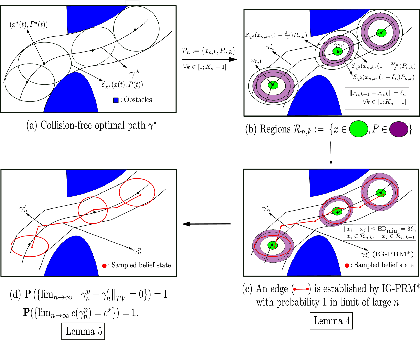
Figure 1: The figure depicts the outline of the proof. (a) Representation of optimal path $\gamma^{\star}$ with cost $c(\gamma^{\star})=c^{\star}$. (c) The zig-zag chain denoted by $\gamma^{p}_{n}$ (red curve) is the chain generated by the IG-PRM* algorithm (Algorithm 1) where $(x_{i},P_{i})$ denote the belief states that are sampled by IG-PRM*. In Lemma 4, we show that an edge is established by IG-PRM* with probability 1 in the limit of large $n$. (d) We show in Lemma 5 that the zig-zag path generated by IG-PRM* converges to the optimal chain $\gamma^{\prime}_{n}$ in the limit of large $n$. Using continuity of cost function (Theorem 1), we show that the cost of the zig-zag chain $\gamma_{n}^{p}$ converges to the optimal cost $c^{\star}$.

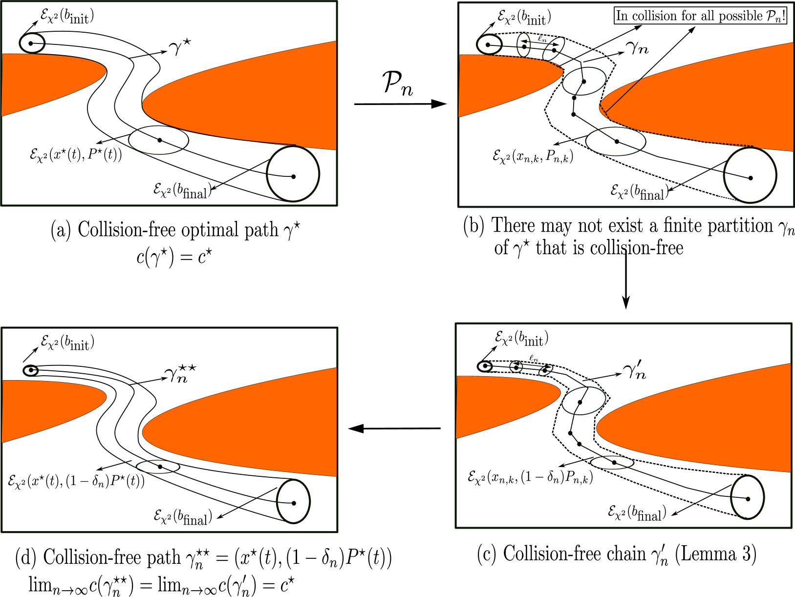
Figure 2: Depiction of different paths $\gamma^{\star}$, $\gamma^{\star\star}_{n}$ and chains $\gamma_{n}$, $\gamma^{\prime}_{n}$ that are used in the proof of asymptotic optimality of IG-PRM*. (a) The optimal path $\gamma^{\star}$ is optimal i.e. $c(\gamma^{\star})=c^{\star}$ and collision-free. (b) From Fig. (2b), there does not exist any partition $\mathcal{P}_{n}$ of the optimal path $\gamma^{\star}$ that would lead to the chain $\gamma_{n}:=\{x_{n,k},P_{n,k}\}$ for all $k\in[1;K_{n}]$ being collision-free (clarified more in Fig. 3). To address this issue, we consider a modified chain $\gamma^{\prime}_{n}:=\{x_{n,k},P^{\prime}_{n,k}\}=\{x_{n,k},(1-\delta_{n})P_{n,k}\}$ for all $k\in[1;K_{n}]$ which is collision-free (Lemma 3). (d) We then show that as the number of samples $n$ tends to infinity, the cost of $\gamma^{\prime}_{n}$ is equal to the cost of $\gamma^{\star\star}_{n}$ i.e. $\underset{n\rightarrow\infty}{\lim}c(\gamma^{\star\star}_{n})=\underset{n\rightarrow\infty}{\lim}c(\gamma^{\prime}_{n})=c^{\star}$ (Eqn. 29).

$$\hat{\mathcal{D}}(b,b^{\prime}):=\|x-x^{\prime}\|,$$ (21a)

$$D_{\text{min}}=3\ell_{n},$$ (21b)

$$\ell_{n}:=\min\left\{\frac{\delta_{n}\sqrt{\chi^{2}\rho}}{16},\frac{\delta_{n}\rho}{18\bar{\sigma}(W)}\right\},$$ (21c)

$$\delta_{n}=\min\left\{\gamma\left(\frac{\text{log}n}{n}\right)^{\frac{2}{d(d+3)}},\frac{1}{2}\right\}$$ (21d)

$$\gamma>\left(\frac{d^{2}+3d+2}{g_{1}g_{2}d(d+3)}\right)^{\frac{2}{d(d+3)}},$$ (21e)

$$g_{1}=\frac{\tau_{d}h^{d}}{\mathcal{V}_{\mathcal{X}}},\;\;\mathcal{V}_{\mathcal{X}}:=\text{vol}(\mathcal{X}),$$ (21f)

$$g_{2}=V_{d}S_{d}(1,1,1/2)2^{-1}(d(d+1))V_{r}^{-1}(2\rho)^{\frac{d(d+1)}{2}}\Delta,$$ (21g)

$$\Delta=\bigg{[}R^{\frac{d(d+1)}{2}}-(\rho d)^{\frac{d(d+1)}{2}}\bigg{]}^{-1},$$ (21h)

$$h:=\min\left\{\frac{\sqrt{\chi^{2}\rho}}{16},\frac{\rho}{18\bar{\sigma}(W)}\right\}=\frac{\ell_{n}}{\delta_{n}}$$ (21i)

The main intuition behind choosing these geometric constants in a certain way is to allow us to prove the asymptotic optimality and would be more clear in subsequent sections. Now, for every belief state $b_{j}$ in $B_{\text{nbors}}$, the function $\operatorname{CollisionFree}(b,b_{j})$ (Line 7 of Algorithm 1) checks that the $\chi^{2}$ confidence bound in transition $b\rightarrow b_{j}$ does not intersect with any obstacles. If the transition $b\rightarrow b_{j}$ is collision-free, an edge is connected between $b$ and $b_{j}$ and stored in $E$. Next, a graph $G$ (Line 9 of Algorithm 1) is constructed using the set of belief states $B$ and the edges $E$. Finally, the shortest path $\gamma_{n}$ (Line 10 of Algorithm 1) between the initial belief $b_{\text{init}}$ to $b_{\text{final}}$ is computed using the Search function (Algorithm 2). Algorithm 2 resembles Algorithm 7 in Choset et al. (2005). The function $\text{Near}_{\text{from}}(G,b_{\text{init}},k)$ finds the $k^{\text{th}}$ nearest nodes in the metric $\hat{D}$ from $G$, to which the transition from $b_{\text{init}}$ are collision-free. Likewise, the function $\text{Near}_{\text{from}}(G,b_{\text{start}},k)$ finds the $k^{\text{th}}$ nearest nodes based on the metric $\hat{D}$ from $G$, from which the transition to $b_{\text{final}}$ is collision-free. The function $\text{ShortestPath}(G,N_{b_{\text{init}}},N_{b_{\text{final}}})$ first uses Dijkstra’s algorithm Dijkstra et al. (1959) to find the shortest path on $G$ between all possible pairs of $b_{1}\in N_{b_{\text{init}}}$ and $b_{2}\in N_{b_{\text{final}}}$, if one exists. Then, this function returns the path that results in the shortest path, among the sought shortest paths, between $b_{\text{init}}$ and $b_{\text{final}}$, or returns Failure if no path is found. However, it must be noted that the belief chain $\gamma_{n}$ computed using the IG-PRM* algorithm (Algorithm 1) might not be finitely lossless. Algorithm 3 ensures that the chain $\gamma_{n}$ is finitely lossless. It takes in as input, $\gamma_{n}$ which consists of say $m$ belief states in sequence. Then for every belief edge $(b_{j-1},b_{j})$ for $j\in[1;m]$, the belief state $b_{j}$ is updated using the function $\operatorname{LosslessRefine}(b_{j-1},b_{j})=(x_{j},P^{\star})$ which ensures that the transition $b_{j-1}\rightarrow b_{j}$ is lossless. In other words, $b_{j}$ now becomes equal to $(x_{j},P^{\star})$. Here, $P^{\star}$ is the minimizer of (2a) computed using Lemma 2. In this case $\hat{P}_{k+1}=P_{j-1}+\|x_{j-1}-x_{j}\|W$ and $P_{k+1}=P_{j}$ where $b_{j-1}\equiv(x_{j-1},P_{j-1})$ and $b_{j}\equiv(x_{j},P_{j})$.

Lemma 2.

[Lemma 1, Pedram et al. (2022)] Let $[U,\Sigma]$ be the eigendecomposition of $P_{k+1}^{-1/2}\hat{P}_{k+1}P_{k+1}^{-1/2}$ i.e. $U\Sigma U^{\top}=P_{k+1}^{-1/2}\hat{P}_{k+1}P_{k+1}^{-1/2}$, where $\Sigma=$ $\operatorname{diag}\left(\sigma_{1},\ldots,\sigma_{n}\right)\succ 0$ and $U$ is unitary matrix. Then, $P^{\star}=$ $P_{k+1}^{1/2}US^{\star}U^{\top}P_{k+1}^{1/2}$ is the optimal solution of (2a) , where $S^{\star}:=$ $\operatorname{diag}\left(\min\left\{1,\sigma_{1}\right\},\ldots,\min\left\{1,\sigma_{\mathrm{n}}\right\}\right)$

Assumption 2.

We assume IG-PRM* is run for $n\geq n^{\star}$, where $n^{\star}$ is the minimum $n^{\prime}\in\mathbb{N}$ such that $\delta_{n^{\prime}}<1/2$.

6 Asymptotic Optimality of IG-PRM*

In this section, we show Algorithm 1 with $D_{\text{min}}$ introduced in Section 5 achieves asymptotic optimality.

6.1 Outline of the proof

Let $\gamma^{\star}:[0,1]\rightarrow\mathbb{R}^{d}\times\mathbb{S}_{\rho}^{d}$, $\gamma^{\star}(t)=(x^{\star}(t),P^{\star}(t))$ be the optimal path and is therefore collision-free by definition (see Fig. (1a)). We define a series of partitions $\mathcal{P}_{n}:=\{x_{n,k},P_{n,k}\}\;k\in[1;K_{n}]$ for $\gamma^{\star}$ where $x_{n,k}=x^{\star}\left(\frac{k-1}{K_{n}}\right)$ and $P_{n,k}:=P\left(\frac{k-1}{K_{n}}\right)$. By construction, $\|x_{n,k+1}-x_{n,k}\|\leq\ell_{n}$ for all $k\in[1;K_{n}-1]$ (see Fig. (1b)).

For each $\mathcal{P}_{n}$, a sequence of regions $\mathcal{R}_{n,k},\;k\in[1;K_{n}]$ is constructed (Section 6.2) which posses three important properties. First, each $\mathcal{R}_{n,k}$ is a region of finite volume. Second, in the limit of large $n$, the volume of these regions converges to zero and the set $\mathcal{R}_{n,k}$ converges to the point $(x_{n,k},P_{n,k})$ for all $k\in[1;K_{n}]$. Last, we show that the transition between consecutive regions i.e., between any belief state $b_{k}\in\mathcal{R}_{n,k}$ and any belief state $b_{k+1}\in\mathcal{R}_{n,k+1}$ is collision-free, and the distance between $b_{k}$ and $b_{k+1}$ is smaller than $D_{\textup{min}}$ (Lemma 3). The main intuition behind the construction of these $\mathcal{R}_{n,k}$, is to show that there is a positive probability that a belief state would be sampled in every $\mathcal{R}_{n,k}$ for $k\in[1;K_{n}]$ by the IG-PRM* algorithm (Algorithm 1) and this would be more clear in subsequent sections. Now, we claim that if the IG-PRM* algorithm is able to sample belief states in every $\mathcal{R}_{n,k}$, the connection between any $b_{k}\in\mathcal{R}_{n,k}$ and $b_{k+1}\in\mathcal{R}_{n,k+1}$ will be established by Algorithm 1, if they are sampled (i.e. if $b_{k}\in B$ and $b_{k+1}\in B$) as shown in Fig. (1c). To prove this mathematically, we define the event $E_{n}\triangleq E_{n,1}\cap E_{n,2}\dots\cap E_{n,K_{n}}$ (Section 6.3) as the event that a belief state is sampled inside all $\mathcal{R}_{n,k}$ regions, and show that the event $E_{n}$ occurs with probability one as $n$ tends to infinity (Lemma 4).

Note that by definition, the optimal path $\gamma^{\star}$ is collision-free. However, the partition chain $\mathcal{P}_{n}$ might not be collision-free as one of the confidence ellipsoids of $\mathcal{P}_{n}$ would pass along the boundary of the obstacle as shown in Fig. 2. To fix this issue, we construct a chain $\gamma_{n}^{\prime}\triangleq(x_{n,k},P^{\prime}_{n,k}:=(1-\delta_{n})P_{n,k}),\;k\in[1;K_{n}]$ (Section 6.4) such that $(x_{n,k},P^{\prime}_{n,k})\in\mathcal{R}_{n,k}$ and thus the transition between $(x_{n,k},P^{\prime}_{n,k})$ to $(x_{n,k+1},P^{\prime}_{n,k+1})$ for $k\in[1;K_{n}-1]$ becomes collision-free. Next, we show that the cost of $\gamma^{\prime}_{n}$ converges to the cost of the optimal path $c^{\star}=c(\gamma^{\star})$ in the limit of large $n$. Now, we need to link the cost of collision-free $\gamma^{\prime}$ to the cost of the feasible paths generated by the IG-PRM* algorithm (Algorithm 1) as we are ultimately interested in analyzing the cost of paths returned by IG-PRM*. To that end, we show there exists a path on the graph generated by the IG-PRM^⋆ algorithm (more precisely, the path generated by connecting sampled nodes in consecutive $\mathcal{R}_{n,k+1}$s) that gets arbitrarily close to $\gamma^{\prime}_{n}$ as $n$ tends to infinity (Lemma 5). Even though the IG-PRM* generated path would get arbitrarily close to $\gamma^{\prime}_{n}$ in the limit of large $n$, it is still not clear whether the cost of these generated paths would tend to $c(\gamma^{\prime}_{n})$ as $n$ tends to infinity. To that end, we leverage the continuity of path cost function (Theorem 1) to show that the cost of that path gets arbitrarily close to $c^{\star}$.

6.2 Construction of collision-free region $\mathcal{R}_{n,k}$

Let $\{\delta_{n}\}$ for $n\in\mathbb{N}$ be a sequence of positive numbers defined in Section 5. Note that $0<\delta_{n}\leq\frac{1}{2}$ for each $n$ and $\underset{n\rightarrow\infty}{\lim}\;\delta_{n}=0$. Let $c^{\star}$ be the optimal path length and

$$\ell^{\star}=\sup_{\mathcal{P}}\sum_{k=1}^{K_{n}-1}\|x^{\star}(t_{k+1})-x^{\star}(t_{k})\|$$

be the total travel length of the optimal path $\gamma^{\star}:[0,1]\rightarrow\mathbb{R}^{d}\times\mathbb{S}^{d},\gamma^{\star}(t)=(x^{\star}(t),P^{\star}(t))$. For each $n\in\mathbb{N}$, choose $\ell_{n}$ as defined in (21c) and $K_{n}=\lceil\frac{\ell^{\star}}{\ell_{n}}\rceil$. Consider the equi-spaced partition $\mathcal{P}_{n}=(0=t_{n,0}\leq t_{n,1}\leq\cdots\leq t_{n,K_{n}}=1)$, and define the chain $\gamma_{n}:=(x_{n,k},P_{n,k})\triangleq(x^{\star}(t_{n,k}),P^{\star}(t_{n,k}))$, $k\in[1;K_{n}]$. By construction, we have $\|x_{n,k+1}-x_{n,k}\|\leq\ell_{n}$ for each $k\in[1;K_{n}-1]$. However, the chain $\gamma_{n}$ constructed this way is not collision-free in general (Fig. 2). To that end, we define regions

$$\mathcal{R}_{n,k}=\{ (x,P):x\in\mathcal{B}(x_{n,k},\ell_{n}),$$

$$\left(1-\frac{3\delta_{n}}{2}\right)P_{n,k}\preceq P\preceq\left(1-\frac{\delta_{n}}{2}\right)P_{n,k}\},$$ (22)

and show that the transition from any $b_{1}\equiv(x_{1},P_{1})\in\mathcal{R}_{n,k}$ to any $b_{2}\equiv(x_{2},P_{2})\in\mathcal{R}_{n,k+1}$ is collision-free. In transition $b_{1}\rightarrow b_{2}$, the mean and covariance of the state can be parameterized as $x[\lambda]=(1-\lambda)x_{1}+\lambda x_{2}$ and $P[\lambda]=P_{1}+\lambda\|x_{2}-x_{1}\|W$ for $\lambda\in[0,1]$.

Remark 3.

The length of minor semi-axis of confidence ellipse $\mathcal{E}_{\chi^{2}}(x,P)$ is $\sqrt{\chi^{2}\underline{\sigma}(P)}$. Consequently, the minimum distance between the boundary of co-centric, similar ellipses $\mathcal{E}_{\chi^{2}}(x,P)$ and $\mathcal{E}_{\chi^{2}}(x,\alpha P)$, where $\alpha>0$, is $\sqrt{\chi^{2}|1-\alpha|\underline{\sigma}(P)}$.

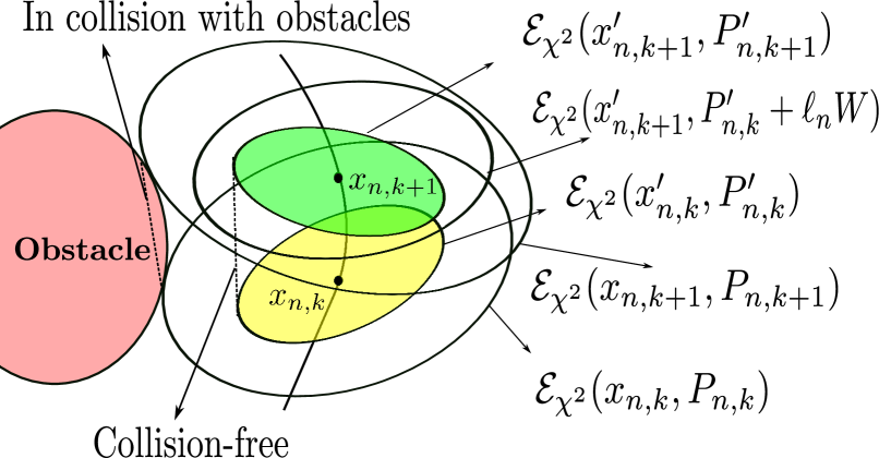
Figure 3: Transition from $(x^{\prime}_{n,k},P^{\prime}_{n,k}:=(1-\delta_{n})P_{n,k})$ to $(x^{\prime}_{n,k+1},P^{\prime}_{n,k+1}:=(1-\delta_{n})P_{n,k+1})$ for all $k\in[1;K_{n}-1]$ is collision-free even if transition from $(x_{n,k},P_{n,k})$ to $(x_{n,k+1},P_{n,k+1})$ is not.

Lemma 3.

In any transition from $b_{1}=(x_{1},P_{1})\in\mathcal{R}_{n,k}$ to $b_{2}=(x_{2},P_{2})\in\mathcal{R}_{n,k+1}$, for all $\lambda\in[0,1]$, $\mathcal{E}_{\chi^{2}}(x[\lambda],P[\lambda])\subset\mathcal{E}_{\chi^{2}}(x_{n,k},P_{n,k})$, for $\ell_{n}:=\min\left\{\frac{\delta_{n}\sqrt{\chi^{2}\rho}}{16},\frac{\delta_{n}\rho}{18\bar{\sigma}(W)}\right\}$. This relation proves that the transition $b_{1}=(x_{1},P_{1})\rightarrow b_{2}=(x_{2},P_{2})$ fully resides in $\mathcal{E}_{\chi^{2}}(x_{n,k},P_{n,k})$, and thus it is collision-free.

Proof.

The proof is provided in two stages. In the first stage, we show

$$P[\lambda]\preceq\left(1-\frac{\delta_{n}}{3}\right)P_{n,k},\quad\forall\lambda\in[0,1].$$ (23)

As the first step to prove (23), we note that

$$||x_{2}-x_{1}||\leq$$

$$||x_{n,k}-x_{1}||+||x_{n,k+1}-x_{n,k}||+||x_{2}-x_{n,k+1}||$$

$$\leq\ell_{n}+\ell_{n}+\ell_{n}=3\ell_{n}=:D_{\text{min}}.$$

Thus, we have

$$P[\lambda] =P_{1}+\lambda||x_{2}-x_{1}||W$$

$$\preceq\left(1-\frac{\delta_{n}}{2}\right)P_{n,k}+||x_{2}-x_{1}||W$$ (24)

$$\preceq\left(1-\frac{\delta_{n}}{2}\right)P_{n,k}+3\ell_{n}W.$$

Hence, to establish (23), it suffices to show

$$\left(1-\frac{\delta_{n}}{2}\right)P_{n,k}+3\ell_{n}W\preceq\left(1-\frac{\delta_{n}}{3}\right)P_{n,k}$$ (25)

Condition (25) is equivalent to

$$3\ell_{n}W \preceq\left[\left(1-\frac{\delta_{n}}{3}\right)-\left(1-\frac{\delta_{n}}{2}\right)\right]P_{n,k}$$

$$=\frac{\delta_{n}}{6}P_{n,k},$$

which trivially holds as $\ell_{n}\leq\frac{\delta_{n}\rho}{18\bar{\sigma}(W)}$. Consequently,

$$\mathcal{E}_{\chi^{2}}(x_{n,k},P[\lambda])\subseteq\mathcal{E}_{\chi^{2}}\left(x_{n,k},\left(1-\frac{\delta_{n}}{3}\right)P_{n,k}\right),$$

for all $\lambda\in[0,1]$. The minimum distance between $\mathcal{E}_{\chi^{2}}(x_{n,k},P_{n,k})$ and $\mathcal{E}_{\chi^{2}}\left(x_{n,k},\left(1-\frac{\delta_{n}}{3}\right)P_{n,k}\right)$ is $\left(1-\sqrt{(1-\frac{\delta_{n}}{3})}\right)\sqrt{\chi^{2}\underline{\sigma}(P_{n,k})}\geq\frac{\delta_{n}}{8}\sqrt{\chi^{2}\underline{\sigma}(P_{n,k})}$. After linear translating $\mathcal{E}\left(x_{n,k},\left(1-\frac{\delta_{n}}{3}\right)P_{n,k}\right)$ for $||x[\lambda]-x_{n,k}||\leq(1-\lambda)\|x_{1}-x_{n,k}\|+\lambda\|x_{2}-x_{n,k}\|\leq(1-\lambda)\ell_{n}+2\lambda(\|x_{2}-x_{n,k+1}\|+\|x_{n,k+1}-x_{n,k}\|)\leq(1+\lambda)\ell_{n}\leq 2\ell_{n}\leq\frac{\delta_{n}}{8}\sqrt{\chi^{2}\rho}\leq\frac{\delta_{n}}{8}\sqrt{\chi^{2}\underline{\sigma}(P_{n,k})}$, the resultant ellipse $\mathcal{E}_{\chi^{2}}\left(x[\lambda],\left(1-\frac{\delta_{n}}{3}\right)P_{n,k}\right)$, stays inside $\mathcal{E}_{\chi^{2}}(x_{n,k},P_{n,k})$. Subsequently, $\mathcal{E}_{\chi^{2}}(x[\lambda],P[\lambda])\subset\mathcal{E}_{\chi^{2}}(x_{n,k},P_{n,k})$. $\hfill\blacksquare$ ■

Finally, we stress that as shown in proof of Lemma 3 the distance $\hat{D}(b_{1},b_{2})$ between any $b_{1}=(x_{1},P_{1})\in\mathcal{R}_{n,k}$ and any $b_{2}=(x_{2},P_{2})\in\mathcal{R}_{n,k+1}$ for all $k\in[1;K_{n}-1]$ is less than $3\ell_{n}:=D_{\text{min}}$ so the connection between $b_{1}$ and $b_{2}$ will be attempted by Algorithm 1.

6.3 Probability of event $E_{n}$

Let $b_{i}:=(x_{i},P_{i})\in B$ be sample belief state by Algorithm 1 at iteration $i$. Then, due to the uniform distribution the probability of event that $x$ is samples inside $\mathcal{B}(x_{n,k},\ell_{n})$ is given by

$$\mathbb{P}(\{x_{i}\in\mathcal{B}(x_{n,k},\ell_{n})\})\! =\!\frac{\text{vol}(\mathcal{B}(x_{n,k},\ell_{n}))}{\text{vol}(\mathcal{X}_{\text{free}})}$$

$$=\frac{\tau_{d}\ell^{d}_{n}}{\mathcal{V}_{\mathcal{X}}}=\frac{\tau_{d}\delta_{n}^{d}h^{d}}{\mathcal{V}_{\mathcal{X}}}=:g_{1}\delta_{n}^{d},\!$$

where $\mathcal{V}_{\mathcal{X}}:=\text{vol}(\mathcal{X}_{\text{free}})$ and $g_{1}:=\frac{\tau_{d}h^{d}}{\mathcal{V}_{\mathcal{X}}}$. If we define

$$\small\mathcal{D}_{n,k}:= \{P\in\mathbb{S}^{d}_{4\rho}:$$

$$\left(1-\frac{3\delta_{n}}{2}\right)P_{n,k}\preceq P\preceq\left(1-\frac{\delta_{n}}{2}\right)P_{n,k}\},$$

we have $\left(1-\frac{3\delta_{n}}{2}\right)P_{n,k}\succeq\left(1-\frac{3}{4}\right)\underline{\sigma}(P_{n,k})I\succeq\rho I$. Thus, Theorem 1 holds in these regions. We have $\textup{Tr}(P)\geq 4(1-\frac{3\delta_{n}}{2})\rho d\geq\rho d$ for all $P\in\mathcal{D}_{n,k}$. On the other hand, $\textup{Tr}(P)\leq(1-\frac{\delta_{n}}{2})\textup{Tr}(P_{n,k})\leq(1-\frac{\delta_{n}}{2})R\leq R$. Hence, $\mathcal{D}_{n,k}\subset\mathcal{R}_{[(1-\frac{3\delta_{n}}{2})4\rho d,(1-\frac{\delta_{n}}{2})R]}\subset\mathcal{R}_{[\rho d,R]}$.

From the definition of uniform sampling, we have

$$\mathbb{P}(P_{i}\in\mathcal{D}_{n,k}){\geq}\frac{\text{vol}(\mathcal{D}_{n,k}\cap\mathcal{D}_{[\rho d,R]})}{\text{vol}(\mathcal{D}_{[\rho d,R]})}=\frac{\text{vol}(\mathcal{D}_{n,k})}{\text{vol}(\mathcal{D}_{[\rho d,R]})}$$

$$=\frac{\text{vol}(\mathcal{D}_{(1-\frac{\delta_{n}}{2})P_{n,k}})-\text{vol}(\mathcal{D}_{(1-\frac{3\delta_{n}}{2})P_{n,k}})}{\text{vol}(\mathcal{R}_{R})-\text{vol}(\mathcal{R}_{\rho d})}$$

$$\geq\frac{V_{d}Sb^{\frac{d(d+1)}{2}}\bigg{[}(1-\frac{\delta_{n}}{2})^{\frac{d(d+1)}{2}}-(1-\frac{3\delta_{n}}{2})^{\frac{d(d+1)}{2}}\bigg{]}}{\left(\frac{2}{d(d+1)}\right)V_{r}\bigg{[}R^{\frac{d(d+1)}{2}}-(\rho d)^{\frac{d(d+1)}{2}}\bigg{]}}.$$

where $S=S_{d}(1,1,1/2)$ and $b=\underset{k\in[1;d]}{\min}\;\lambda_{k}(P_{n,k})$.

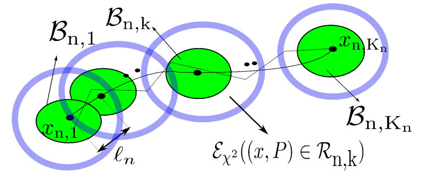
Figure 4: Covering of chain $\gamma_{n}$ with balls of radius $\ell_{n}$. The event $E_{n,k}$ is the event that a sampled point $(x,P)\in\mathcal{R}_{n,k}$.

Now, we have

$$\left(1-\frac{\delta_{n}}{2}\right)^{\frac{d(d+1)}{2}}-\left(1-\frac{3\delta_{n}}{2}\right)^{\frac{d(d+1)}{2}}$$

$$=\bigg{(}\left(1-\frac{\delta_{n}}{2}\right)-\left(1-\frac{3\delta_{n}}{2}\right)\bigg{)}$$

$$\qquad\sum_{j=0}^{\frac{d(d+1)}{2}-1}\left(1-\frac{\delta_{n}}{2}\right)^{\frac{d(d+1)}{2}-1-j}\left(1-\frac{3\delta_{n}}{2}\right)^{j}$$

$$\geq\delta_{n}d\left(1-\frac{3\delta_{n}}{2}\right)^{\frac{d(d+1)}{2}-1}\geq d\left(\frac{\delta_{n}}{2}\right)^{\frac{d(d+1)}{2}},$$

where in the last step we use $\delta_{n}\leq 1/2$. In sum, it can be deduced

$$\mathbb{P}(P_{i}\in\mathcal{D}_{n,k})\geq g_{2}\delta_{n}^{\frac{d(d+1)}{2}},$$ (26)

where $g_{2}=V_{d}S_{d}(1,1,1/2)2^{-1}(d(d+1))V_{r}^{-1}(2\rho)^{\frac{d(d+1)}{2}}\bigg{[}R^{\frac{d(d+1)}{2}}-(\rho d)^{\frac{d(d+1)}{2}}\bigg{]}^{-1}$ is a constant.

Lets define the event $E^{i}_{n,k}$ is as the event that the sampled belief $b_{i}=(x_{i},P_{i})$ belongs to $\mathcal{R}_{n,k}$. Then, $E_{n,k}=\cup_{i=1}^{n}E^{i}_{n,k}$ which means the event that $\mathcal{R}_{n,k}$ contains at least one sample belief $b_{i}\in B$. The following lemma shows that if the $\gamma$ is greater than a certain positive threshold, then the probability that event $E_{n}\triangleq E_{n,1}\cap E_{n,2}\dots\cap E_{n,K_{n}}$ occurs, i.e the event that all $R_{n,k}$’s contain at least one sampled belief, equals to one as $n$ approaches infinity.

Lemma 4.

If $\gamma>\left(\frac{d^{2}+3d+2}{g_{1}g_{2}d(d+3)}\right)^{\frac{2}{d(d+3)}}$, then the following holds true

$$\underset{n\rightarrow\infty}{\lim}\;\mathbb{P}\left(E_{n}\right)=1.$$

Proof.

The probability of event $E^{c}_{n,k}$ for all $k\in[1;K_{n}]$ is given as follows:

$$\mathbb{P}\left(E^{c}_{n,k}\right)=\prod_{i=1}^{n}(1-\mathbb{P}\left(E^{i}_{n,k}\right))$$

$$\leq\left(1-\mathbb{P}(P\in\mathcal{D}_{n,k})\;\mathbb{P}(x\in\mathcal{B}_{n,k})\right)^{n}$$

$$\leq\left[1-g_{2}\delta_{n}^{d}g_{1}\delta_{n}^{\frac{d(d+1)}{2}}\right]^{n}=\left[1-g_{1}g_{2}\delta_{n}^{\frac{d(d+3)}{2}}\right]^{n}.$$

Using the fact that $(1-x)\leq e^{-x}$ for $x\in(0,1)$, and substituting $\delta_{n}$ defined as

$$\delta_{n}=\min\;\left\{\gamma\left(\frac{\text{log}n}{n}\right)^{\frac{2}{d(d+3)}},\frac{1}{2}\right\},$$

we have

$$\mathbb{P}\left(E^{c}_{n,k}\right) \leq\left(1-g_{1}g_{2}{\gamma^{\frac{d(d+3)}{2}}\frac{\text{log}n}{n}}\right)^{n}$$

$$\leq\text{exp}\left(-(\log n)g_{1}g_{2}\gamma^{\frac{d(d+3)}{2}}\right)=n^{-g_{1}g_{2}\gamma^{\frac{d(d+3)}{2}}}.$$

Now, the event $E_{n}^{c}=\bigcup_{k=1}^{n}E^{c}_{n,k}$ is upper bounded as follows:

$$\mathbb{P}\left(E^{c}_{n}\right) \!=\!\mathbb{P}\left(\bigcup_{k=1}^{K_{n}}E^{c}_{n,k}\right)\!\leq\!\sum_{k=1}^{K_{n}}\mathbb{P}\left(E^{c}_{n,k}\right)\!\leq\!K_{n}n^{-g_{1}g_{2}\gamma^{\frac{d(d+3)}{2}}}.$$

where $K_{n}=\lfloor\frac{\ell^{\star}}{\ell_{n}}\rfloor\leq\frac{\ell^{\star}}{\ell_{n}}$. Since $\delta_{n}h\leq\ell_{n}$, we have

$$\mathbb{P}\left(E^{c}_{n}\right) \leq\frac{\ell^{\star}}{h\delta_{n}}n^{-g_{1}g_{2}\gamma^{\frac{d(d+3)}{2}}}$$

$$=\frac{\ell^{\star}}{\gamma h}(\log n)^{-\frac{2}{d(d+3)}}n^{-g_{1}g_{2}\gamma^{\frac{d(d+3)}{2}}+\frac{2}{d(d+3)}}.$$ (27)

If the power of $n$ in (27) is less than $-1$, which is equivalent to

$$\gamma>\left(\frac{d^{2}+3d+2}{g_{1}g_{2}d(d+3)}\right)^{\frac{2}{d(d+3)}},$$

we have $\sum_{n=1}^{\infty}\mathbb{P}\left(E^{c}_{n}\right)<\infty$. Consequently, $\underset{n\rightarrow\infty}{\lim}\mathbb{P}\left(E^{c}_{n}\right)=1$, by Borel Cantelli lemma Grimmett and Stirzaker (2020) which completes the proof. $\hfill\blacksquare$ ■

6.4 Construction of chain $\gamma^{\prime}_{n,k}$

For each $n\in\mathbb{N}$, define a collision-free path $\gamma_{n}^{\star\star}:[0,1]\rightarrow\mathbb{R}^{d}\times\mathbb{S}_{\rho}^{d}$ by $\gamma_{n}^{\star\star}(t)=(x^{\star}(t),(1-\delta_{n})P^{\star}(t))$ (See Figure 2). It is trivial to check $\underset{n\rightarrow\infty}{\lim}\gamma^{\star\star}_{n}=\gamma^{\star}$ and thus $\underset{n\rightarrow\infty}{\lim}c(\gamma^{\star\star}_{n})=c^{\star}$.

We define a chain $\gamma^{\prime}_{n}:=(x_{n,k},(1-\delta_{n})P_{n,k})$, $k\in[1;K_{n}]$, which is the chain generated by partition $\mathcal{P}_{n}$ on path $\gamma_{n}^{\star\star}(t)$. It is easy to verify that $(x_{n,k},(1-\delta_{n})P_{n,k})\in\mathcal{R}_{n,k}$. Thus, from Lemma 3 one can deduce that $\gamma^{\prime}_{n}$ is collision-free. Using $\{(x_{n,k},P^{\prime}_{n,k}=(1-\delta_{n})P_{n,k})\}_{k=1}^{K_{n}}$, we define path $\widetilde{\gamma}_{n}(t)=(\widetilde{x}_{n}(t),\widetilde{P}_{n}(t))$ as

$$\widetilde{x}_{n}(t) =\frac{t_{n,k+1}-t}{t_{n,k+1}-t_{n,k}}x_{n,k}+\frac{t-t_{n,k}}{t_{n,k+1}-t_{n,k}}x_{n,k+1}$$

$$\widetilde{P}_{n}(t) =P^{\prime}_{n,k}+\|\tilde{x}_{n}(t)-x^{\prime}_{n,k}\|W$$

for $t_{n,k}\leq t<t_{n,k+1},k\in[1;K_{n}-1]$ with $\widetilde{x}(1)=x_{n,K_{n}}$, $\widetilde{P}(1)=P^{\prime}_{n,K_{n}}$. Notice that we have

$$c^{\star}\leq c(\widetilde{\gamma}_{n})=c(\gamma^{\prime}_{n})\leq c(\gamma^{\star\star}_{n})$$ (28)

since $\widetilde{\gamma}_{n}$ is collision-free path from initial belief state to the goal region (the first inequality) and

$$c(\gamma^{\prime}_{n})=c(\gamma^{\star\star}_{n};\mathcal{P}_{n})\leq\sup_{\mathcal{P}}c(\gamma^{\star\star}_{n};\mathcal{P})=c(\gamma^{\star\star}_{n}).$$ (29)

Since $\underset{n\rightarrow\infty}{\lim}c(\gamma^{\star\star}_{n})=c^{\star}$, (28) implies $\underset{n\rightarrow\infty}{\lim}c(\gamma^{\prime}_{n})=c^{\star}$.

6.5 Convergence to optimal path $\gamma^{\star}$

In subsection 6.3, we showed $\underset{n\rightarrow\infty}{\lim}\;\mathbb{P}\left(E_{n}\right)=1$. In this subsection, we assume $E_{n}$ has occurred and show almost surely $G$ contains a path whose cost is arbitrarily close to $c^{\star}$ in the limit of large $n$. Let the set of paths generated by the IG-PRM* algorithm be denoted by $P_{n}$ and let $\gamma^{p}_{n}$ be closest to $\gamma^{\prime}_{n}$ in terms of bounded variation i.e., $\gamma^{p}_{n}=\underset{\gamma^{p}\in P_{n}}{\operatorname*{argmin}}\;\|\gamma^{p}-\gamma^{\prime}_{n}\|_{TV}$. Then, we have the following lemma.

Lemma 5.

$\mathbb{P}\left(\left\{\underset{n\rightarrow\infty}{\lim}\;\left\|\gamma^{p}_{n}-\gamma^{\prime}_{n}\right\|_{TV}=0\right\}\right)=1$

Proof.

Define set $\mathcal{R}^{\beta}_{n,k}\subseteq\mathcal{R}_{n,k}$

$$\mathcal{R}^{\beta}_{n,k}=\Biggl{\{}(x,P):x\in\mathcal{B}\left(x_{n,k},\beta\ell_{n}\right),$$

$${\left(1-\delta_{n}-\beta\frac{\delta_{n}}{2}\right)}P_{n,k}\preceq P\preceq\left(1-\delta_{n}+\beta\frac{\delta_{n}}{2}\right)P_{n,k}\Biggl{\}},$$

where $0<\beta\leq 1$. Define $I_{n,k}$ as follows:

$$I_{n,k}:=\begin{cases}1,&\text{ if }\mathcal{R}^{\beta}_{n,k}\cap V^{\mathrm{IG-PRM}^{*}}=\emptyset,\\ 0,&\text{ otherwise. }\end{cases}$$ (30)

We define $M_{n}=\sum_{k=1}^{K_{n}}I_{n,k}$, and examine the event $\{M_{n}\leq\alpha K_{n}\}$ which means the event that at least $\alpha$ fraction of all $K_{n}$ regions (i.e., $R_{n,k}$s regions) do not contain any sampled belief $b_{i}\in B$. If $\mathcal{R}^{\beta}_{n,k}$ contains a sampled belief state $(x,P)$, we have

$$\|x-x_{n,k}\| \leq\beta\ell_{n},$$

$$\|P-P_{n,k}\|_{F} \leq\|(1-\delta_{n}+\beta\frac{\delta_{n}}{2})P_{n,k}-(1-\delta_{n})P_{n,k}\|_{F}$$

$$\leq\left((1-\delta_{n}+\beta\frac{\delta_{n}}{2})-(1-\delta_{n})\right)\|P_{n,k}\|_{F}$$

$$\leq\beta\frac{\delta_{n}}{2}\|P_{n,k}\|_{F}$$

$$\leq\beta\frac{\delta_{n}}{2}\|P_{n,k}\|_{F}\leq\beta\frac{R}{2h}\ell_{n},$$

which yields $\hat{\mathcal{D}}((x,P),(x_{n,k},P_{n,k}))\leq\beta c\ell_{n}$, where $c:=1+R/2h$. For $k$’s that no sample belief is inside $\mathcal{R}^{\beta}_{n,k}$, we can assume there exists a sampled belief $(x,P)$ inside $\mathcal{R}_{n,k}$, because we have assumed $E_{n}$ has occurred. For such $k$s, we have $\hat{\mathcal{D}}((x,P),(x_{n,k},P_{n,k}))\leq c\ell_{n}$ because $\mathcal{R}_{n,k}=\mathcal{R}^{\beta=1}_{n,k}$. Considering the path generated by connecting the sampled belief in consequent $\mathcal{R}^{\beta}_{n,k}$ or $\mathcal{R}_{n,k}$ regions, we have

$$\left\|\gamma^{p}_{n}-\gamma^{\prime}_{n}\right\|_{TV} \leq\sum_{k=1}^{K_{n}}\hat{\mathcal{D}}((x,P),(x_{n,k},P_{n,k})$$

$$\leq K_{n}(\alpha c\ell_{n}+(1-\alpha)\beta c\ell_{n})$$

$$\leq c(\alpha+\beta)L,$$ (31)

where $L=\underset{n\in\mathbb{N}}{\sup}\;\gamma^{\prime}_{n}$. Therefore,

$$\left\{M_{n}\leq\alpha K_{n}\right\}\subseteq\left\{\left\|\gamma^{p}_{n}-\gamma^{\prime}_{n}\right\|_{TV}\leq c(\alpha+\beta)L\right\}.$$

Taking the complement of both sides of above equation and using the monotonicity of probability measures,

$$\mathbb{P}\left(\!\left\{\left\|\gamma^{p}_{n}-\gamma^{\prime}_{n}\right\|_{TV}\!>\!c(\alpha+\beta)L\right\}\!\right)\!\leq\!\mathbb{P}\left(\!\left\{M_{n}\!\geq\!\alpha K_{n}\right\}\!\right).$$ (32)

Since (32) is true for any $\alpha,\beta\in(0,1)$, it remains to show that $\mathbb{P}\left(\left\{M_{n}\geq\alpha K_{n}\right\}\right)$ converges to zero. Let’s denote $\ell^{\beta}_{n,k}:=\beta\ell_{n})$, $\mathcal{D}^{\beta}_{n,k}=\{P\succ 0:{(1-\delta_{n}-\beta\frac{\delta_{n}}{2})}P_{n,k}\preceq P\preceq(1-\delta_{n}+\beta\frac{\delta_{n}}{2})P_{n,k}\}$. Then, expected value of $I_{n,m}$ can be computed as

$$\mathbb{E}[I_{n,m}]=\mathbb{P}(\{I_{n,m}=1\})$$

$$\leq\left(1-\mathbb{P}(x\in\mathcal{B}(x,\ell^{\beta}_{n,k}))\times\mathbb{P}(P\in\mathcal{D}^{\beta}_{n,k})\right)^{n}$$

$$\leq\left(1-g_{1}\beta^{d}\delta^{d}_{n}\times g_{2}\beta\delta_{n}^{\frac{d(d+1)}{2}}\right)^{n}$$

$$=\left(1-g_{1}g_{2}\beta^{d+1}\delta_{n}^{\frac{d(d+3)}{2}}\right)^{n}$$

$$\leq\text{exp}\left(-ng_{1}g_{2}\beta^{d+1}\delta_{n}^{\frac{d(d+3)}{2}}\right)$$

$$=\text{exp}\left(-g_{1}g_{2}\beta^{d+1}\gamma^{\frac{d(d+3)}{2}}\frac{\log n}{n}n\right)$$

$$\leq\text{exp}\left(-\frac{-g_{1}g_{2}\beta^{d+1}(d^{2}+3d+2)}{d(d+3)}\log n\right)$$

$$=n^{\frac{-\beta^{d+1}g_{1}g_{2}(d^{2}+3d+2)}{d(d+3)}}.$$

Thus, $\mathbb{E}[M_{n}]=\sum_{m=1}^{K_{n}}\mathbb{E}[I_{n,m}]=K_{n}n^{\frac{-\beta^{d+1}g_{1}g_{2}(d^{2}+3d+2)}{d(d+3)}}$. By Markov’s inequality, it follows that

$$\mathbb{P}\left(\left\{M_{n}\geq\alpha K_{n}\right\}\right) \leq\frac{\mathbb{E}[M_{n}]}{\alpha K_{n}}\leq\frac{K_{n}n^{\frac{-\beta^{d+1}g_{1}g_{2}(d^{2}+3d+2)}{d(d+3)}}}{\alpha K_{n}}$$

$$=\frac{n^{\frac{-\beta^{d+1}g_{1}g_{2}(d^{2}+3d+2)}{d(d+3)}}}{\alpha}.$$

it is trivial to verify that for fixed $\alpha$, the last expression tends to $0$ as $n$ tends to $\infty$. Since this argument holds for all small $\alpha,\beta$, (32) implies for all $\epsilon>0$,

$$\mathbb{P}\left(\left\{\underset{n\rightarrow\infty}{\lim}\;\left\|\gamma^{p}_{n}-\gamma^{\prime}_{n}\right\|_{TV}=0\right\}\right)=1.$$

$\hfill\blacksquare$ ■

As shown in Subsection 6.4 $\underset{n\rightarrow\infty}{\lim}c(\gamma^{\prime}_{n})=c^{\star}$. Using this result, the fact that $\mathbb{P}\left(\left\{\underset{n\rightarrow\infty}{\lim}\;\left\|\gamma^{p}_{n}-\gamma^{\prime}_{n}\right\|_{TV}=0\right\}\right)=1$, and the continuity of the cost function (Theorem 1), we can conclude that $\mathbb{P}(\{\underset{n\rightarrow\infty}{\lim}c(\gamma^{p}_{n})=c^{\star}\})=1.$

7 Loss-less version of IG-PRM*

Note that only lossless transitions between edges of a feasible path are meaningful for physical systems Pedram et al. (2022). However, the path generated by IG-PRM* (Algorithm 1) is not guaranteed to be finitely lossless. Although there exists an analytical solution to perform lossless refinement (Algorithm 3) for the entire path using the information geometric cost defined in (3), an analytical solution might not exist for other information metrics such as Hellinger or Wasserstein. To address this limitation, we propose the finitely lossless version of the IG-PRM* algorithm termed Lossless IG-PRM* (Algorithm 4) where the edge between two belief states is guaranteed to be finitely lossless and is devoid of any lossless refinement step. In addition, we prove the asymptotic optimality of Lossless IG-PRM*.

Algorithm 4 represents the pseudocode for the Lossless IG-PRM*. The function $\operatorname{CollisionFree}(b,b_{j},\chi^{2})$ checks whether the edge from belief state $b$ to $b_{j}$ is collision-free. The function $\operatorname{Lossless}(b,b_{j})$ checks whether the transition from $b$ to $b_{j}$ is lossless. The search algorithm (Algorithm 2) is used to compute the lossless and collision-free chain $\gamma^{\prime\prime}_{n}$.

1 $\left.B\leftarrow\left\{b_{\text{init}}\right\}\cup\{\text{SampleFree}_{i}\right\}_{i\in[1;n]};E\leftarrow\emptyset$;

2 for $b\in B$ do

3       $\quad B_{\text{nbors}}\leftarrow\operatorname{Near}\left(B,b,D_{\text{min}}\right)$;

4       for $b_{j}\in B_{\text{nbors}}$ do

5             if $\operatorname{CollisionFree}(b,b_{j},\chi^{2})\;\operatorname{and}\;\operatorname{Lossless}(b,b_{j})$  then

6                  $E\leftarrow E\cup\{(b,b_{j})\}$;

7            

8      

return $G=(B,E)$

Algorithm 4 Lossless IG-PRM*

Towards the aim of proving asymptotic optimality, we define modified $\ell^{L}_{n},\;\mathcal{R}^{L}_{n,k},\;\mathcal{D}^{L}_{n,k},\;\mathcal{R}^{L,s}_{n,k},\;\mathcal{R}^{L,\beta s}_{n,k}$ and $\delta^{L}_{n}$ as follows:

$$\ell^{L}_{n}:=\min\left\{\delta^{L}_{n}\left(1-\frac{3}{4}\delta^{L}_{n}\right)\frac{\rho}{3\bar{\sigma}(W)},{\frac{\delta^{L}_{n}}{9}\rho},{\frac{\delta^{L}_{n}}{3}\chi^{\frac{1}{4}}{\rho}^{\frac{1}{8}}},q_{n}\right\},$$

$$\quad\geq\delta^{L}_{n}h^{L}$$

$$\mathcal{B}^{s}(x_{n,k},\ell^{L}_{n}):=\mathcal{B}(x_{n,k},\frac{(1-(\theta^{1}_{n,k})^{2})}{2}(\ell^{L}_{n})^{4})$$

$$\mathcal{R}^{L}_{n,k}=\{(x,P):x\in\mathcal{B}(x_{n,k},(\ell^{L}_{n})^{4}),P\preceq{\left(\theta^{0}_{n,k}\right)^{2}}P^{\prime\prime}_{n,k}\}$$

$$\mathcal{R}^{L,s}_{n,k}=\{(x,P):x\in\mathcal{B}^{s}(x_{n,k},\ell^{L}_{n})\},$$

$$\mathcal{D}^{L}_{n,k}:=\{P\succeq 0:{(\theta^{1}_{n,k})^{2}}P^{\prime\prime}_{n,k}\preceq P\preceq{(\theta^{2}_{n,k})^{2}}P^{\prime\prime}_{n,k}\},$$

$$\;\quad\quad{(\theta^{1}_{n,k})^{2}}P^{\prime\prime}_{n,k}\preceq P\preceq{(\theta^{2}_{n,k})^{2}}P^{\prime\prime}_{n,k},\}$$

$$\mathcal{R}^{L,\beta s}_{n,k}=\Biggl{\{}(x,P):x\in\mathcal{B}\left(x_{n,k},\frac{\beta(1-(\theta^{1}_{n,k})^{2})}{2}(\ell^{L}_{n})^{4}\right),$$

$${(\beta\theta^{1}_{n,k}+(1-\beta)\theta^{2}_{n,k})^{2}}P^{\prime\prime}_{n,k}\preceq P\preceq{(\theta^{2}_{n,k})^{2}}P^{\prime\prime}_{n,k}\Biggl{\}}$$

$$\delta^{L}_{n}=\min\;\left\{\gamma\left(\frac{\text{log}n}{n}\right)^{\frac{1}{d(2d+8)}},1\right\}$$

where $q_{n}=\min\left\{\frac{\delta_{n}\sqrt{\chi^{2}\rho}}{16},\frac{\delta_{n}\rho}{18\bar{\sigma}(W)}\right\},\;\theta^{1}_{n,k}=\theta^{2}_{n}-(k+1)\Delta$, $\theta^{2}_{n,k}=\theta^{2}_{n}-k\Delta$, and $\Delta=(\theta^{2}_{n}-\theta^{1}_{n})/K^{L}_{n}$. Here, $\theta^{2}_{n}:=\sqrt{{1}-\frac{\ell^{2}_{n}}{\chi^{\frac{1}{2}}\rho^{\frac{1}{4}}}}$, and $\theta^{1}_{n}:=\sqrt{1-(\delta^{L}_{n})^{2}+\frac{\ell^{2}_{n}}{\chi^{\frac{1}{2}}\rho^{\frac{1}{4}}}}$, $h^{L}:=\min\left\{\frac{\rho}{12\bar{\sigma}(W)},\frac{\rho}{9},\frac{\rho^{\frac{1}{4}}}{3}\right\}$ and $\beta\in(0,1)$ where $\theta^{0}_{n,k}$ is defined as follows

$$\theta_{n,k}^{0}=1-\frac{(\ell^{L}_{n})^{4}}{\sqrt{\chi^{2}\underline{\sigma}(P^{\prime\prime}_{n,k})}}$$

The outline of the asymptotic optimality proof is as follows. The quantities $\gamma^{\star}$, $\gamma^{\star}(t)$, $\gamma_{n}^{\prime}$ and $\mathcal{P}_{n}$ are same as that described in Section 6.1. However, for Lossless IG-PRM*, in addition to proving that the entire path is collision-free, we also need to show that the path is finitely lossless. This necessitates us to modify some constants and regions compared to that mentioned in Section 6.1 and the mathematical reason behind it would be clear in subsequent sections. As $\gamma_{n}^{\prime}$ might not be finitely lossless, we first consider the lossless refinement of $\gamma_{n}^{\prime}$ to obtain a finitely lossless and collision-free chain $\gamma_{n}^{\prime\prime}\triangleq(x_{n,k},P^{\prime\prime}_{n,k}),\;k\in[1;K^{L}_{n}]$ and show the cost of $\gamma^{\prime\prime}$ converges to the cost of the optimal path $c^{\star}=c(\gamma^{\star})$ in the limit of $n$ tending to infinity.

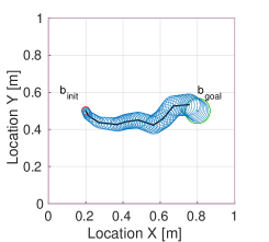
(a) $c(\gamma_{n})=1.12$

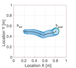
(b) $c(\gamma_{n})=0.90$

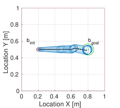
(c) $c(\gamma_{n})=0.61$

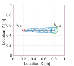
(d) $c^{\star}=0.60$

Figure 5: Figs. (a), (b) and (c) are the paths computed by IG-PRM* after 2000, 8000, and 15000 iterations respectively. (d) The optimal path generated in the absence of obstacles from initial belief state $b_{\text{init}}$ to final belief state $b_{\text{goal}}$ using the move and sense strategy presented in Pedram et al. (2022).

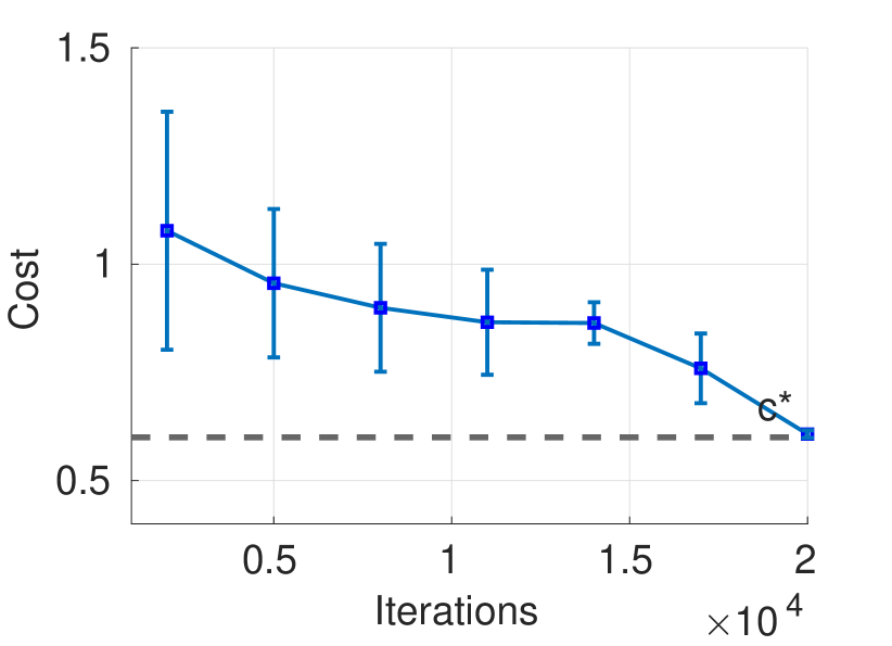
Figure 6: The plot shows the convergence of the cost computed by IG-PRM* algorithm to the optimal cost $c^{\star}=0.60$ as the number of samples $n$ increases.

To draw the connection between $\gamma^{\prime\prime}_{n}$ and the cost of paths returned by the Lossless IG-PRM* algorithm (Algorithm 4), the regions $\mathcal{R}^{L}_{n,k}$ are constructed in such a way that the transition between consecutive regions i.e., between any belief state $b_{k}\in\mathcal{R}^{L}_{n,k}$ and any belief state $b_{k+1}\in\mathcal{R}^{L}_{n,k+1}$ for all $k\in[1;K^{L}_{n}-1]$ is collision-free. However, as the edge connecting $b_{k}\in\mathcal{R}^{L}_{n,k}$ to any belief state $b_{k+1}\in\mathcal{R}^{L}_{n,k+1}$ might not be lossless, we define a region $\mathcal{R}^{L,s}_{n,k}$ which is a subset of $\mathcal{R}^{L}_{n,k}$ and show the transition between any $b^{s}_{k}\in\mathcal{R}^{L,s}_{n,k}$ to any $b^{s}_{k+1}\in\mathcal{R}^{L,s}_{n,k+1}$ is both lossless and collision-free (Lemma 8). Furthermore, we show that the distance between $b_{k}$ and $b_{k+1}$ is smaller that $D_{\textup{min}}$ (Lemma 9). However, it is still not clear whether a connection between $b_{k}^{s}$ and $b_{k+1}^{s}$ will be established by Algorithm 4, if $b^{s}_{k}\in B$ and $b^{s}_{k+1}\in B$. To prove this mathematically, we define event $E_{n}\triangleq E_{n,1}\cap E_{n,2}\dots\cap E_{n,K^{L}_{n}}$ as the event that a belief state is sampled inside all $\mathcal{R}^{L,s}_{n,k}$ regions, and show that the event $E_{n}$ occurs with probability one as $n$ tends to infinity (Lemma 10). We then show there exists a path on the graph generated by the Lossless IG-PRM^⋆ algorithm that gets arbitrarily close to $\gamma^{\prime\prime}_{n}$ as $n$ tends to infinity (Lemma 11). Finally, we leverage the continuity of path cost function to show that the cost of that path returned by Lossless IG-PRM* gets arbitrarily close to $c^{\star}$ (Lemma 12).

Lemma 6.

The chain $\gamma^{\prime}_{n}=(x_{n,k},P^{\prime}_{n,k})\triangleq(x^{\star}(t_{n,k}),(1-\delta^{L}_{n})^{2}P^{\star}(t_{n,k}))\triangleq(x_{n,k},P^{\prime}_{n,k})\triangleq(x_{n,k},(1-\delta^{L}_{n})^{2}P_{n,k})$, $k\in[1;K_{n}]$ is collision-free.

Proof.

Please see Appendix C ■

Lemma 7.

In any transition from $(x_{1},P_{1})\in\mathcal{R}^{L}_{n,k}$ $(x_{2},P_{2})\in\mathcal{R}^{L}_{n,k+1}$, both initial confidence ellipse and final confidence ellipse are contained inside $\mathcal{E}_{\chi^{2}}(x_{n,k},P_{n,k})$. More precisely,

$$\mathcal{E}_{\chi^{2}}(x_{1},P_{1})\subseteq\mathcal{E}_{\chi^{2}}(x_{n,k},P_{n,k}),$$ (33)

$$\mathcal{E}_{\chi^{2}}(x_{2},P_{1}+||x_{2}-x_{1}||W)\subseteq\mathcal{E}_{\chi^{2}}(x_{n,k},P_{n,k}),$$ (34)

which proves the transition $(x_{1},P_{1})\rightarrow(x_{2},P_{2})$ fully resides in $\mathcal{E}_{\chi^{2}}(x_{n,k},P_{n,k})$, and thus it is collision-free.

Proof.

Please see Appendix D. ■

Lemma 8.

The transition between any state $(x_{1},P_{1})\in\mathcal{R}^{L,s}_{n,k}$ to $(x_{2},P_{2})\in\mathcal{R}^{L,s}_{n,k+1}$ for all $k\in[1;K_{n}-1]$ is finitely lossless and collision-free.

Proof.

Please see Appendix E. ■

Lemma 9.

The distance $\hat{D}(b_{1},b_{2})$ between any $b_{1}=(x_{1},P_{1})\in\mathcal{R}^{L,s}_{n,k}$ and any $b_{2}=(x_{2},P_{2})\in\mathcal{R}^{L,s}_{n,k+1}$ for all $k\in[1;K_{n}-1]$ is less than $D_{\text{min}}$.

Proof.

Please see Appendix F. ■

Lemma 10.

If $\gamma>\left(\frac{d(2d+8)+1}{g^{L}_{1}g^{L}_{2}d(2d+8)}\right)^{\frac{1}{d(2d+8)}}$, then $\underset{n\rightarrow\infty}{\lim}\;\mathbb{P}\left(E_{n}\right)=1$.

Proof.

Please see Appendix G. ■

Lemma 11.

$\mathbb{P}\left(\left\{\underset{n\rightarrow\infty}{\lim}\;\left\|\gamma^{p}_{n}-\gamma^{\prime\prime}_{n}\right\|_{TV}=0\right\}\right)=1$

Proof.

Please see Appendix H. ■

Lemma 12.

$\mathbb{P}(\{\underset{n\rightarrow\infty}{\lim}c(\gamma^{p}_{n})=c^{\star}\})=1$

Proof.

Please see Appendix I. ■

8 Numerical Experiments

We consider a scenario with no obstacles and verify that Algorithm 1 converges to the analytically computed cost as the number of samples increases.

8.1 Obstacle free space

In obstacle-free space, we compute the optimal solution to (3) by using Theorem 1 in Pedram et al. (2022). We then use the IG-PRM* algorithm (Algorithm 1) to plot the cost returned as the number of samples $n$ increases. The obstacle-free space considered is of dimension $1\mathrm{m}\times 1\mathrm{m}$ with initial belief state $b_{\text{init}}:=(x_{\text{init}},P_{\text{init}})$ and goal belief state $b_{\text{goal}}:=(x_{\text{goal}},P_{\text{goal}})$ where $x_{\text{init}},\;P_{\text{init}},\;x_{\text{goal}}$ and $P_{\text{goal}}$ are defined as

$$x_{\text{init}}=[0.2,\;0.5]^{\mathrm{T}},\quad x_{\text{goal}}=[0.8,\;0.5]^{\mathrm{T}}$$

$$P_{\text{init}}=10^{-4}I,\quad P_{\text{goal}}=10^{-3}I$$

We perform a total of 70 experiments where the IG-PRM* is run for iterations $i=2000+3000m$ for $m\in[0;6]$ and for each $m$, 10 experiments were performed. The average cost is calculated and the results are depicted as an error plot as shown in Fig. 6. From Fig. 6, it can be observed that the cost returned by IG-PRM* converges to the optimal cost $c^{\star}$ as the number of samples increases. Fig. 5 shows the evolution of the path as the number of samples increases.

9 Conclusion and Future Work

In this paper, we proposed a sampling based motion planning algorithm in Gaussian belief space termed IG-PRM* that minimizes the information geometric cost and proved that the algorithm converges to the optimal solution as the number of samples tends to infinity. We then proposed a variant of IG-PRM* termed Lossless IG-PRM* which does not require lossless modification and prove that the algorithm is asymptotically optimal. In the future, we plan to reduce the computational burden for the IG-PRM* and explore methods to increase the rate of converge of the cost computed by IG-PRM*

This work was supported in part by the Lockheed Martin Corporation under Grant MRA16-005-RPP009, in part by the Air Force Office of Scientific Research under Grant FA9550-20-1-0101,

Appendix A Proof of Theorem 3

We adopt the eigenvalue decomposition to parameterize $P\in\mathbb{S}^{d}_{+}$ as

$$P(\Lambda,U)=U^{\top}\Lambda U,$$

where $\Lambda=\textup{diagonal}(\lambda_{1},\dots,\lambda_{d})$ and $U$ is a $d\times d$ real orthonormal matrix (i.e., $UU^{\top}=U^{\top}U=I_{d}$). Using this parametrization, referred to as polar parametrization, we can express the volume element $dP$ as

$$dP=\det\theta\;\prod_{i<j}^{d}|\lambda_{i}-\lambda_{j}|\prod_{i}^{d}d\lambda_{i},$$

where $\theta_{ij}=\sum_{k=1}^{d}U_{jk}dU_{ik}$ and $\det\theta$ is the exterior product $\det(\theta)=\wedge_{i<j}\theta_{i,j}$ Terras (2012); Mathai (1997). The integral of any function $f:\mathbb{S}^{d}_{+}\rightarrow\mathbb{R}$ over $\mathbb{S}^{d}_{+}$ can be computed using polar parametrization as:

$$\int_{\mathbb{S}^{d}_{+}}f(P)dP=(d!\;2^{d})^{-1}\int_{O(d)}\int_{\mathbb{R}^{d}_{+}}\bigg{(}$$

$$f(P(\Lambda,U))\det\theta\;\prod_{i<j}^{d}|\lambda_{i}-\lambda_{j}|\bigg{)}\prod_{i=1}^{d}d\lambda_{i}.$$ (35)

where $O(d)$ is space of $d\times d$ real orthonormal matrices. The factor $(d!\;2^{d})^{-1}$ in (35) resolves the ambiguity of all possible orderings of $\lambda_{1},\dots,\lambda_{d}$ and all possible orientation (multiplication by $+1$ or $-1$) of the columns of $U$. The volume of $\mathcal{D}_{A}$ can be computed by substituting the indicator function of $\mathcal{D}_{A}$ in place of $f(P(\Lambda,U))$ in (35). Thus,

$$\textup{Vol}(\mathcal{D}_{A})$$

$$= \int_{O(d)}\int_{\Lambda\preceq A}\bigg{(}\det\theta\;\prod_{i<j}^{d}|\lambda_{i}-\lambda_{j}|\bigg{)}\prod_{i=1}^{d}d\lambda_{i}$$

$$\geq\textup{Vol}(\mathcal{D}^{\prime}_{A})$$

$$= (d!\;2^{d})^{-1}\left(\int_{O(d)}\det\theta\right)$$

$$\left(\int_{0\leq\lambda_{i}\leq\underset{k\in[1;d]}{\min}a_{k}}\prod_{i<j}^{d}|\lambda_{i}-\lambda_{j}|\prod_{i}^{d}d\lambda_{i}\right)$$

It is a well-known result (see e.g., (Muirhead, 2009, page 71) or Chikuse (2003) ) that $\int_{O(d)}\det\theta=\frac{2^{d}\pi^{d^{2}/2}}{\Gamma_{d}(d/2)}$, where $\Gamma_{d}$ is the gamma function. To compute the integral

$$\int_{0\leq\lambda_{i}\leq\underset{k\in[1;d]}{\min}a_{k}}\prod_{i<j}^{d}|\lambda_{i}-\lambda_{j}|\;\prod_{i}^{d}d\lambda_{i},$$ (36)

we use the transformation $y_{i}=\lambda_{i}/b$ where $b=\underset{k\in[1;d]}{\min}\;a_{k}$. Therefore, $\prod_{i=1}^{d}dy_{i}=\prod_{i=1}^{d}\lambda_{i}/b^{d}$. Consequently, the integral (36) becomes

$$\int_{0\leq y_{i}\leq 1}\prod_{i<j}^{d}|y_{i}-y_{j}|\;\prod_{i}^{d}dy_{i}$$

$$=b^{\frac{d(d+1)}{2}}\int_{0\leq y_{i}\leq 1}\prod_{i<j}^{d}|y_{i}-y_{j}|\;\prod_{i}^{d}dy_{i}$$

$$=b^{\frac{d(d+1)}{2}}S_{d}(1,1,1/2)$$ (37)

where $S_{d}(\alpha_{1},\alpha_{2},\alpha_{3})$ is the Selberg integral Grafakos and Morpurgo (1999) given by

$$S_{d}(\alpha_{1},\alpha_{2},\alpha_{3})$$

$$=\int_{0}^{1}..\int_{0}^{1}\prod_{i=1}^{d}t_{i}^{\alpha_{1}-1}\left(1-t_{i}\right)^{\alpha_{2}-1}\prod_{1\leq i<j\leq d}\left|t_{i}-t_{j}\right|^{2\alpha_{3}}dt$$

$$=\prod_{j=0}^{d-1}\frac{\Gamma(\alpha_{1}+j\alpha_{3})\Gamma(\alpha_{2}+j\gamma)\Gamma(1+(j+1)\gamma)}{\Gamma(\alpha_{1}+\alpha_{2}+(d+j-1)\alpha_{3})\Gamma(1+\alpha_{3})}$$

which results to (18). Now, for $\beta>1$, we have

$$\frac{\textup{Vol}(\mathcal{D}_{\beta A})}{\textup{Vol}(\mathcal{D}_{A})}$$

$$=\frac{\int_{O(d)}\int_{\Lambda\preceq\beta A}\bigg{(}\det\theta\;\prod_{i<j}^{d}|\lambda_{i}-\lambda_{j}|\bigg{)}\prod_{i=1}^{d}d\lambda_{i}}{\int_{O(d)}\int_{\Lambda\preceq A}\bigg{(}\det\theta\;\prod_{i<j}^{d}|\lambda_{i}-\lambda_{j}|\bigg{)}\prod_{i=1}^{d}d\lambda_{i}}$$ (38)

Substituting $z_{i}=\lambda_{i}/\beta$, we have

$$\frac{\textup{Vol}(\mathcal{D}_{\beta A})}{\textup{Vol}(\mathcal{D}_{A})}$$

$$=\frac{\beta^{\frac{d(d+1)}{2}}\int_{O(d)}\int_{\Lambda\preceq A}\bigg{(}\det\theta\;\prod_{i<j}^{d}|z_{i}-z_{j}|\bigg{)}\prod_{i=1}^{d}dz_{i}}{\int_{O(d)}\int_{\Lambda\preceq A}\bigg{(}\det\theta\;\prod_{i<j}^{d}|\lambda_{i}-\lambda_{j}|\bigg{)}\prod_{i=1}^{d}d\lambda_{i}}$$

$$=\beta^{\frac{d(d+1)}{2}}$$ (39)

Furthermore, we have the following

$$\frac{\textup{Vol}(\mathcal{D}^{\prime}_{\beta A})}{\textup{Vol}(\mathcal{D}^{\prime}_{A})}=\frac{\int_{0\leq\lambda_{i}\leq\beta b}\prod_{i<j}^{d}|\lambda_{i}-\lambda_{j}|\;\prod_{i}^{d}d\lambda_{i}}{\int_{0\leq\lambda_{i}\leq b}\prod_{i<j}^{d}|\lambda_{i}-\lambda_{j}|\;\prod_{i}^{d}d\lambda_{i}}$$ (40)

Consider the change of variable as $b_{i}=\lambda_{i}/\beta$. Then, (40) becomes

$$\frac{\textup{Vol}(\mathcal{D}^{\prime}_{\beta A})}{\textup{Vol}(\mathcal{D}^{\prime}_{A})} =\frac{\beta^{\frac{d(d+1)}{2}}\int_{0\leq b_{i}\leq a_{i}}\prod_{i<j}^{d}|b_{i}-b_{j}|\;\prod_{i}^{d}db_{i}}{\int_{0\leq\lambda_{i}\leq a_{i}}\prod_{i<j}^{d}|\lambda_{i}-\lambda_{j}|\;\prod_{i}^{d}d\lambda_{i}}$$

$$=\beta^{\frac{d(d+1)}{2}}=\frac{\textup{Vol}(\mathcal{D}_{\beta A})}{\textup{Vol}(\mathcal{D}_{A})}$$ (41)

Subtracting 1 from both sides of (41), we get

$$\frac{\textup{Vol}(\mathcal{D}_{\beta A})-\textup{Vol}(\mathcal{D}_{A})}{\textup{Vol}(\mathcal{D}_{A})}=\frac{\textup{Vol}(\mathcal{D}^{\prime}_{\beta A})-\textup{Vol}(\mathcal{D}^{\prime}_{A})}{\textup{Vol}(\mathcal{D}^{\prime}_{A})}$$

$$\geq\textup{Vol}(\mathcal{D}^{\prime}_{\beta A})-\textup{Vol}(\mathcal{D}^{\prime}_{A})$$

$$=(\beta^{\frac{d(d+1)}{2}}-1)\textup{Vol}(\mathcal{D}^{\prime}_{A})$$

$$\geq(\beta^{\frac{d(d+1)}{2}}-1)b^{\frac{d(d+1)}{2}}S_{d}(1,1,1/2)$$ (42)

and hence the result follows.

Appendix B Proof of Lemma 1

$\textup{Vol}(\mathcal{D}_{P})$ can be computed by substituting the indicator function of $\mathcal{D}_{P}$ in place of $f(P(\Lambda,U))$ in (35). If we introduce a transformation of variables from $U$ to $U^{\prime}=UV^{\top}$, the Jacobian of the transformation is $1$, and the integral becomes the $\textup{vol}(\mathcal{D}_{\Sigma})$ in the $(\theta^{\prime},P)$ coordinate system. $\hfill\blacksquare$

Appendix C Proof of Lemma 6

To show that the transition from $(x_{n,k},P^{\prime}_{n,k})$ to $(x_{n,k+1},P^{\prime}_{n,k+1})$ is collision-free, it is sufficient to show that

$$\mathcal{E}_{\chi^{2}}(x_{n,k+1},P^{\prime}_{n,k}+\ell^{L}_{n}W)\subset\mathcal{E}_{\chi^{2}}(x_{n,k},P_{n,k}).$$ (43)

In what follows, we derive a sufficient condition for $\ell^{L}_{n}$ to satisfy (43). Suppose that $\ell^{L}_{n}$ is small enough so that

$$P^{\prime}_{n,k}+\ell^{L}_{n}W\preceq P^{\prime}_{n,k}+3\ell^{L}_{n}W\preceq\left(1-\frac{\delta^{L}_{n}}{2}\right)^{2}P_{n,k}$$ (44)

holds. (44) is equivalent to

$$(1-\delta^{L}_{n})^{2}P_{n,k}+\ell^{L}_{n}W \preceq(1-\delta^{L}_{n})^{2}P_{n,k}+3\ell^{L}_{n}W$$

$$\preceq\left(1-\frac{\delta^{L}_{n}}{2}\right)^{2}P_{n,k}$$

or

$$3\ell^{L}_{n}W\preceq\delta^{L}_{n}\left(1-\frac{3}{4}\delta^{L}_{n}\right)P_{n,k}.$$ (45)

which trivially holds as $\ell^{L}_{n}\leq\delta^{L}_{n}\left(1-\frac{3}{4}\delta^{L}_{n}\right)\frac{\rho}{3\bar{\sigma}(W)}$. In order for (44) to imply (43), we further require the distance $\|x_{n,k+1}-x_{n,k}\|$ between the centers of two ellipses in (43) is less than or equal to the difference between semi-minor axis lengths of ellipses characterized by $P_{n,k}$ and $(1-\frac{\delta^{L}_{n}}{2})^{2}P_{n,k}$ computed as $\frac{\delta^{L}_{n}}{2}\sqrt{\chi^{2}\underline{\sigma}(P_{n,k})}$. Notice that $\|x_{n,k+1}-x_{n,k}\|\leq\ell^{L}_{n}\leq 3\ell^{L}_{n}$. On the other hand, the difference between the semi-minor axis lengths is greater than $\frac{\delta^{L}_{n}}{2}\sqrt{\chi^{2}\rho}$. Therefore, if

$$\ell^{L}_{n}\leq\frac{\delta^{L}_{n}}{6}\sqrt{\chi^{2}\rho}$$ (46)

then (44) implies (43). To summarize, since $\ell^{L}_{n}$ simultaneously satisfies (44) and (46), (43) holds. $\hfill\blacksquare$

Appendix D Proof of Lemma 7

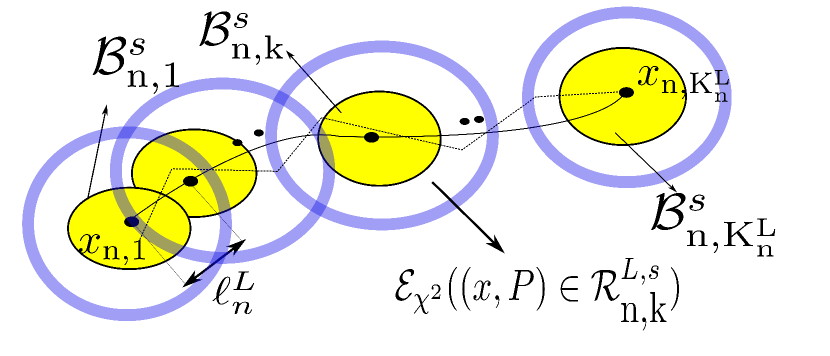
Figure 7: Covering of collision-free and lossless chain $\gamma^{\prime\prime}_{n}$ with balls $\mathcal{B}^{s}_{n,k}$ of radius $\frac{(1-(\theta^{1}_{n,k})^{2})}{2}\ell^{L}_{n}$. The event $E_{n,k}$ is the event that a sampled point $(x,P)\in\mathcal{R}^{L,s}_{n,k}$.

Lets define $\mathcal{E}^{\text{out}}_{n,k}:=\mathcal{E}_{\chi^{2}}(x_{n,k},{(\theta^{0}_{n,k})^{2}}P^{\prime\prime}_{n,k})$, it is easy to verify that the minimum distance $\mathcal{E}^{\text{out}}_{n,k}$ and $\mathcal{E}_{\chi^{2}}(x_{n,k},P^{\prime\prime}_{n,k})$ is $(\ell^{L}_{n})^{4}$. On the other hand, any translation of the center of ellipsoid $\mathcal{E}^{\text{out}}_{n,k}$ from $x_{n,k}$ to some $x\in\mathcal{B}(x_{n,k},(\ell^{L}_{n})^{4})$, will linearly translate the ellipsoid $\mathcal{E}_{\chi^{2}}\left(x_{n,k},P\right)$ by a maximum of distance $(\ell^{L}_{n})^{4}$. Thus, after the translation the ellipse stays inside $\mathcal{E}(x_{n,k},P^{\prime\prime}_{n,k})\subset\mathcal{E}(x_{n,k},P_{n,k})$ and (33) holds. As the first step to prove (34), we stress that

$$||x_{2}-x_{1}||\leq$$

$$||x_{n,k}-x_{1}||+||x_{n,k+1}-x_{n,k}||+||x_{2}-x_{n,k+1}||$$

$$\leq(\ell^{L}_{n})^{4}+(\ell^{L}_{n})^{4}+(\ell^{L}_{n})^{4}\leq\ell^{L}_{n}+\ell^{L}_{n}+\ell^{L}_{n}=3\ell^{L}_{n}.$$

Thus, we have

$$P_{1}+||x_{2}-x_{1}||W \preceq P^{\prime\prime}_{n,k}+||x_{2}-x_{1}||W$$

$$\preceq P^{\prime}_{n,k}+||x_{2}-x_{1}||W\preceq P^{\prime}_{n,k}+3\ell^{L}_{n}W$$

$$\preceq\left(1-\frac{\delta^{L}_{n}}{2}\right)^{2}P_{n,k},$$ (47)

where the last inequality is shown earlier as (44). From (47), we have

$$\mathcal{E}(x_{n,k},P_{1}+||x_{2}-x_{1}||W)\subseteq\mathcal{E}\left(x_{n,k},\left(1-\frac{\delta^{L}_{n}}{2}\right)^{2}P_{n,k}\right).$$

The minimum distance between $\mathcal{E}(x_{n,k},P_{n,k})$ and $\mathcal{E}\left(x_{n,k},\left(1-\frac{\delta^{L}_{n}}{2}\right)^{2}P_{n,k}\right)$ is $\frac{\delta^{L}_{n}}{2}\sqrt{\chi^{2}\underline{\sigma}(P_{n,k})}$, Thus after linear translating $\mathcal{E}\left(x_{n,k},\left(1-\frac{\delta^{L}_{n}}{2}\right)^{2}P_{n,k}\right)$ for $||x_{2}-x_{n,k}||\leq\|x_{2}-x_{n,k+1}\|+\|x_{n,k}-x_{n,k+1}\|\leq 2\ell^{L}_{n}\leq\frac{\delta^{L}_{n}}{2}\sqrt{\chi^{2}\rho}\leq\frac{\delta^{L}_{n}}{2}\sqrt{\chi^{2}\underline{\sigma}(P_{n,k})}$, the resultant ellipse $\mathcal{E}_{\chi^{2}}(x_{2},\left(1-\frac{\delta^{L}_{n}}{2}\right)^{2}P_{n,k})$, and subsequently $\mathcal{E}_{\chi^{2}}\left(x_{2},P_{1}+||x_{2}-x_{1}||W\right)$ stays inside $\mathcal{E}_{\chi^{2}}\left(x_{n,k},P_{n,k}\right)$.$\hfill\blacksquare$

Appendix E Proof of Lemma 8

We know that the chain $(x_{n,k},P^{\prime\prime}_{n,k})$ for all $k\in[1;K^{L}_{n}]$ is lossless and collision-free. Therefore,

$$P^{\prime\prime}_{n,k+1}\preceq P^{\prime\prime}_{n,k}+\ell^{L}_{n}W$$ (48)

for all $k\in[1;K^{L}_{n}-1]$. Further, since sampled point $(x_{2},P_{2})\in\mathcal{R}^{L,s}_{n,k+1}$, the following is true

$$(\theta^{1}_{n,k+1})^{2}P^{\prime\prime}_{n,k+1}\preceq P_{2}\preceq{(\theta^{2}_{n,k+1}})^{2}P^{\prime\prime}_{n,k+1}$$

$$\implies\frac{P_{2}}{(\theta^{2}_{n,k+1})^{2}}\preceq P^{\prime\prime}_{n,k+1}\preceq\frac{P_{2}}{(\theta^{1}_{n,k+1})^{2}}$$ (49)

Using (48) and (49), $\frac{P_{2}}{(\theta^{2}_{n,k+1})^{2}}\preceq P^{\prime\prime}_{n,k}+\ell^{L}_{n}W$. Further, using the fact that $\theta^{1}_{n,k}=\theta^{2}_{n,k+1}$ for $k\in[1;K^{L}_{n}-1]$ implies the following

$${P_{2}} \preceq{(\theta^{2}_{n,k+1})^{2}}P^{\prime\prime}_{n,k}+{(\theta^{2}_{n,k+1})^{2}}\ell^{L}_{n}W$$

$$={(\theta^{1}_{n,k})^{2}}P^{\prime\prime}_{n,k}+{(\theta^{1}_{n,k})^{2}}\ell^{L}_{n}W$$

$$\preceq P_{1}+{(\theta^{1}_{n,k})^{2}}\ell^{L}_{n}W\preceq P_{1}+\frac{((\theta^{1}_{n,k+1})^{2}+(\theta^{1}_{n,k})^{2})}{2}\ell^{L}_{n}W$$

Using the fact that $\|x_{n,k+1}-x_{n,k}\|=\ell^{L}_{n}$, $(x_{1},P_{1})\in\mathcal{R}^{L,s}_{n,k}$ and $(x_{2},P_{2})\in\mathcal{R}^{L,s}_{n,k+1}$, the minimum distance between $x_{2}$ and $x_{1}$ is given as

$$\|x_{2}-x_{1}\| \geq\ell^{L}_{n}-\frac{(1-(\theta^{1}_{n,k})^{2})}{2}(\ell^{L}_{n})^{4}$$

$$-\frac{(1-(\theta^{1}_{n,k+1})^{2})}{2}(\ell^{L}_{n})^{4}$$

$$\geq\frac{(\theta^{1}_{n,k+1})^{2}+(\theta^{1}_{n,k})^{2}}{2}\ell^{L}_{n}.$$

Consequently, $P_{2}\preceq P_{1}+\|x_{2}-x_{1}\|W$. Therefore, $P_{2}\preceq P_{1}+\|x_{2}-x_{1}\|W$. Further, since $\mathcal{R}^{L,s}_{n,k+1}\subset\mathcal{R}^{L}_{n,k+1}$ by construction, the edge between two sampled points $(x_{1},P_{1})\in\mathcal{R}^{L,s}_{n,k}$ and $(x_{2},P_{2})\in\mathcal{R}^{L,s}_{n,k+1}$ for all $k\in[1;K^{L}_{n}-1]$ is finitely lossless and collision-free.$\hfill\blacksquare$

Appendix F Proof of Lemma 9

We first note that the maximum distance between $x_{2}$ and $x_{1}$ is

$$\|x_{2}-x_{1}\| \leq\ell^{L}_{n}+\frac{(1-(\theta^{1}_{n,k})^{2})}{2}(\ell^{L}_{n})^{4}+$$

$$\frac{(1-(\theta^{1}_{n,k+1})^{2})}{2}(\ell^{L}_{n})^{4}$$

$$\leq\left(2-\frac{(\theta^{1}_{n,k+1})^{2}+(\theta^{1}_{n,k})^{2}}{2}\right)\ell^{L}_{n}\leq 2\ell^{L}_{n}.$$

Therefore, we have $\hat{D}(b_{1},b_{2})=\|x_{2}-x_{1}\|\leq 2\ell^{L}_{n}:=D_{\text{min}}$.

Appendix G Proof of Lemma 10

Then, due to the uniform distribution, $\mathbb{P}(\{x_{i}\in\mathcal{B}(x_{n,k},(\ell^{L}_{n})^{4})\})$ is given by

$$\mathbb{P}(\{x_{i}\in\mathcal{B}(x_{n,k},(\ell^{L}_{n})^{4})\}) =\frac{\text{vol}(\mathcal{B}(x_{n,k},(\ell^{L}_{n})^{4}))}{\text{vol}(\mathcal{X}_{\text{free}})}$$

$$=\frac{\tau_{d}(\ell^{L})^{4d}_{n}}{\mathcal{V}_{\mathcal{X}}}\geq\frac{\tau_{d}(\delta^{L}_{n})^{4d}(h^{L})^{4d}}{\mathcal{V}_{\mathcal{X}}},$$

where $\mathcal{V}_{\mathcal{X}}:=\text{vol}(\mathcal{X}_{\text{free}})$. It is straightforward to verify that

$$\mathbb{P}(\{x_{i}\in\mathcal{B}^{s}(x_{n,k},\ell^{L}_{n})\})\! =\!c_{n,k}\mathbb{P}(\{x_{i}\in\mathcal{B}(x_{n,k},(\ell^{L}_{n})^{4})\})$$

$$\geq\frac{\tau_{d}(\delta^{L}_{n})^{6d}(h^{L})^{6d}}{\mathcal{V}_{\mathcal{X}}\chi^{\frac{d}{2}}\rho^{\frac{d}{4}}2^{d}}=g^{L}_{1}(\delta^{L}_{n})^{6d}$$

where $g^{L}_{1}:=\frac{\tau_{d}(h^{L})^{6d}}{\mathcal{V}_{\mathcal{X}}\chi^{\frac{d}{2}}\rho^{\frac{d}{4}}2^{d}}$. We have $\textup{Tr}(P)\geq 16(\theta^{1}_{n,k})^{2}\rho d\geq\rho d$ for all $P\in\mathcal{D}_{n,k}$. On the other hand, $\textup{Tr}(P)\leq(\theta^{2}_{n,k})^{2}\textup{Tr}(P^{\prime\prime}_{n,k})\leq(\theta^{2}_{n,k})^{2}R\leq R$. Hence, $\mathcal{D}_{n,k}\subset\mathcal{R}_{[(\theta^{1}_{n,k})^{2}16\rho d,(\theta^{2}_{n,k})^{2}R]}\subset\mathcal{R}_{[\rho d,R]}$.

From the definition of uniform sampling, we have

$$\mathbb{P}(P_{i}\in\mathcal{D}_{n,k}){\geq}\frac{\text{vol}(\mathcal{D}_{n,k}\cap\mathcal{D}_{[\rho d,R]})}{\text{vol}(\mathcal{D}_{[\rho d,R]})}=\frac{\text{vol}(\mathcal{D}_{n,k})}{\text{vol}(\mathcal{D}_{[\rho d,R]})}$$

$$=\frac{\text{vol}(\mathcal{D}_{(\theta^{2}_{n,k})^{2}P^{\prime\prime}_{n,k}})-\text{vol}(\mathcal{D}_{(\theta^{1}_{n,k})^{2}P^{\prime\prime}_{n,k}})}{\text{vol}(\mathcal{R}_{R})-\text{vol}(\mathcal{R}_{\rho d})}$$

$$\geq\frac{V_{d}S_{d}(1,1,1/2)b^{\frac{d(d+1)}{2}}\bigg{[}(\theta^{2}_{n,k})^{d(d+1)}-(\theta^{1}_{n,k})^{d(d+1)}\bigg{]}}{\left(\frac{2}{d(d+1)}\right)V_{r}\bigg{[}R^{\frac{d(d+1)}{2}}-(\rho d)^{\frac{d(d+1)}{2}}\bigg{]}}.$$

where $b=\underset{i\in[1;d]}{\min}\;\lambda_{i}(P^{\prime\prime}_{n,k})$. Now, we have

$$(\theta^{2}_{n,k})^{d(d+1)}-(\theta^{1}_{n,k})^{d(d+1)}$$

$$=(\theta^{2}_{n,k}-\theta^{1}_{n,k})\sum_{j=0}^{d(d+1)-1}(\theta^{2}_{n,k})^{d-1-j}(\theta^{1}_{n,k})^{j}$$

$$\geq d\frac{(\theta^{2}_{n}-\theta^{1}_{n})}{K^{L}_{n}}(\theta^{1}_{n})^{d(d+1)-1}$$

$$\geq d\frac{(\theta^{2}_{n}-\theta^{1}_{n})}{2K^{L}_{n}}(\theta^{2}_{n}+\theta^{1}_{n})(\theta^{1}_{n})^{d(d+1)-1}$$

$$\geq d\frac{\ell^{L}_{n}}{2\ell^{\star}}(\delta^{L}_{n})^{2}\left(1-\frac{(\delta_{n}^{L})^{2}}{9}\right)^{d(d+1)-1}$$

$$\geq\frac{h^{L}d}{\ell^{\star}}\left(\frac{\delta^{L}_{n}}{3}\right)^{2d(d+1)}.$$

where in the last step we use $\delta^{L}_{n}\leq 1$. In sum, it can be deduced

$$\mathbb{P}(P_{i}\in\mathcal{D}_{n,k})\geq g^{L}_{2}(\delta^{L}_{n})^{2d(d+1)},$$ (50)

where $g^{L}_{2}=\frac{V_{d}V_{r}^{-1}S_{d}(1,1,1/2)2^{-1}d^{2}(d+1)h^{L}(16\rho)^{\frac{d(d+1)}{2}}}{\ell^{\star}3^{2d(d+1)}}\bigg{[}R^{\frac{d(d+1)}{2}}-(\rho d)^{\frac{d(d+1)}{2}}\bigg{]}^{-1}$ is a constant.

Lets define the event $E^{i}_{n,k}$ is as the event that the sampled belief $b_{i}=(x_{i},P_{i})$ belongs to $\mathcal{R}^{s}_{n,k}$. Then, $E_{n,k}=\cup_{i=1}^{n}E^{i}_{n,k}$. The following lemma shows that if the $\gamma$ is greater than a certain positive threshold, then the probability that event $E_{n}\triangleq E_{n,1}\cap E_{n,2}\dots\cap E_{n,K^{L}_{n}}$ occurs equals to one as $n$ approaches infinity. The probability of event $E^{c}_{n,k}$ for all $k\in[1;K^{L}_{n}]$ is given as follows:

$$\mathbb{P}\left(E^{c}_{n,k}\right)=\prod_{i=1}^{n}(1-\mathbb{P}\left(E^{i}_{n,k}\right))$$

$$\leq\left(1-\mathbb{P}(P\in\mathcal{D}_{n,k})\;\mathbb{P}(x\in\mathcal{B}_{n,k})\right)^{n}\leq$$

$$\leq\left[1-g^{L}_{1}(\delta^{L}_{n})^{6d}g^{L}_{2}(\delta^{L}_{n})^{2d(d+1)}\right]^{n}$$

$$=\left[1-g^{L}_{1}g^{L}_{2}(\delta^{L}_{n})^{d(2d+8)}\right]^{n}.$$

Using the fact that $(1-x)\leq e^{-x}$ for $x\in(0,1)$, and substituting $\delta^{L}_{n}$, for sufficiently large $n$, we have

$$\mathbb{P}\left(E^{c}_{n,k}\right) \leq\left(1-g^{L}_{1}g^{L}_{2}{\gamma^{d(2d+8)}\frac{\text{log}n}{n}}\right)^{n}\leq n^{-g^{L}_{1}g^{L}_{2}\gamma^{d(2d+8)}}.$$

Now, the event $E_{n}^{c}=\bigcup_{k=1}^{n}E^{c}_{n,k}$ is upper bounded as follows:

$$\mathbb{P}\left(E^{c}_{n}\right) \!=\!\mathbb{P}\left(\bigcup_{k=1}^{K^{L}_{n}}E^{c}_{n,k}\right)\!\leq\!\sum_{k=1}^{K^{L}_{n}}\mathbb{P}\left(E^{c}_{n,k}\right)\!\leq\!K^{L}_{n}n^{-g^{L}_{1}g^{L}_{2}\gamma^{d(2d+8)}}.$$

where $K^{L}_{n}=\lfloor\frac{\ell^{\star}}{\ell^{L}_{n}}\rfloor\leq\frac{\ell^{\star}}{\ell^{L}_{n}}$. Since $\delta^{L}_{n}h^{L}\leq\ell^{L}_{n}$, we have

$$\mathbb{P}\left(E^{c}_{n}\right)\leq\frac{\ell^{\star}}{\delta^{L}_{n}h^{L}}n^{-g^{L}_{1}g^{L}_{2}\gamma^{d(2d+8)}}$$

$$=\frac{\ell^{\star}}{\delta^{L}_{n}h^{L}}(\log n)^{-\frac{1}{d(2d+8)}}n^{-g^{L}_{1}g^{L}_{2}\gamma^{d(2d+8)}+\frac{1}{d(2d+8)}}.$$ (51)

If the power of $n$ in (51) is less than $-1$, which is equivalent to

$$\gamma>\left(\frac{d(2d+8)+1}{g^{L}_{1}g^{L}_{2}d(2d+8)}\right)^{\frac{1}{d(2d+8)}},$$

we have $\sum_{n=1}^{\infty}\mathbb{P}\left(E^{c}_{n}\right)<\infty$. Consequently, $\underset{n\rightarrow\infty}{\lim}\mathbb{P}\left(E^{c}_{n}\right)=1$, by Borel Cantelli lemma Grimmett and Stirzaker (2020) which completes the proof. $\hfill\blacksquare$

Appendix H Proof of Lemma 11

Define $I_{n,k}$ as follows:

$$I_{n,k}:=\begin{cases}1,&\text{ if }\mathcal{R}^{L,\beta s}_{n,k}\cap V^{\mathrm{Lossless\;IG-PRM}^{*}}=\emptyset,\\ 0,&\text{ otherwise. }\end{cases}$$

Define $M_{n}=\sum_{k=1}^{K^{L}_{n}}I_{n,k}$, and assume the event $\{M_{n}\leq\alpha K^{L}_{n}\}$ has occurred which means that $\alpha$ fraction of the $K^{L}_{n}$ points be such that the sampled points do not belong to any $\mathcal{R}^{L,\beta s}_{n,k}$. If the sampled $(x,P)$ is not inside $\mathcal{R}^{L,\beta s}_{n,k}$ but it is inside $\mathcal{R}^{L,s}_{n,k}$, we have

$$\|x-x_{n,k}\|\leq \frac{(1-(\theta^{1}_{n,k})^{2})}{2}(\ell^{L}_{n})^{4}\leq\frac{1}{2}\ell^{L}_{n},$$

$$\|P-P^{\prime\prime}_{n,k}\|_{F} \leq\|(\theta^{1}_{n,k})^{2}P^{\prime\prime}_{n,k}-P^{\prime\prime}_{n,k}\|_{F}$$

$$\leq\|(\theta^{1}_{n})^{2}P^{\prime\prime}_{n,k}-P^{\prime\prime}_{n,k}\|_{F}\leq\frac{16\bar{\rho}\sqrt{d}}{\rho}\ell^{L}_{n},$$

which yields $\hat{\mathcal{D}}((x,P),(x_{n,k},P^{\prime\prime}_{n,k}))\leq c\ell^{L}_{n}$, where $c:=\frac{1}{2}+\frac{16\bar{\rho}\sqrt{d}}{\rho}$. Similarly, if the sampled $(x,P)$ is inside $\mathcal{R}^{L,\beta s}_{n,k}$ we have

$$\|x-x_{n,k}\|\leq\beta\frac{(1-(\theta^{1}_{n,k})^{2})}{2}(\ell^{L}_{n})^{4}\leq\frac{1}{2}\beta\ell^{L}_{n},$$

$$\|P-P^{\prime\prime}_{n,k}\|_{F}$$

$$\leq\|(\beta\theta^{1}_{n,k}+(1-\beta)\theta^{2}_{n,k})^{2}P^{\prime\prime}_{n,k}-(\theta^{2}_{n,k})^{2}P^{\prime\prime}_{n,k}\|_{F}$$

$$+\|(\theta^{2}_{n,k})^{2}P^{\prime\prime}_{n,k}-P^{\prime\prime}_{n,k}\|$$

$$\leq 2\|(\beta\theta^{1}_{n,k}+(1-\beta)\theta^{2}_{n,k})P^{\prime\prime}_{n,k}-\theta^{2}_{n,k}P^{\prime\prime}_{n,k}\|_{F}$$

$$+\|(\theta^{2}_{n,k})^{2}P^{\prime\prime}_{n,k}-P^{\prime\prime}_{n,k}\|$$

$$\leq 2\beta(\theta^{2}_{n,k}-\theta^{1}_{n,k})\|P^{\prime\prime}_{n,k}\|_{F}+\|(\theta^{2}_{n,k})^{2}P^{\prime\prime}_{n,k}-P^{\prime\prime}_{n,k}\|$$

$$\leq 2\beta\Delta\bar{\rho}\sqrt{d}+(\delta^{L}_{n})^{2}\bar{\rho}\sqrt{d}$$

which yields $\hat{\mathcal{D}}((x,P),(x_{n,k},P^{\prime\prime}_{n,k}))\leq 2\beta\Delta\bar{\rho}\sqrt{d}+(\delta^{L}_{n})^{2}\bar{\rho}\sqrt{d}$. If we define $c_{1}:=\beta\bar{\rho}\sqrt{d}$ and $c_{2}=\bar{\rho}\sqrt{d}$ (which is bounded), we have

$$\left\|\gamma^{p}_{n}-\gamma^{\prime\prime}_{n}\right\|_{TV} \leq\sum_{k=1}^{K^{L}_{n}}\hat{\mathcal{D}}((x,P),(x_{n,k},P^{\prime\prime}_{n,k})$$

$$\leq K^{L}_{n}(\alpha c\ell^{L}_{n}+(1-\alpha)\beta c_{1}\Delta+c_{2}(\delta^{L}_{n})^{2})$$

$$\leq c\alpha L+c_{1}\beta(\theta^{2}_{n}-\theta^{1}_{n})+c_{2}\delta^{L}_{n}L/h^{L},$$ (52)

where $L=\underset{n}{\sup}\;\gamma^{\prime\prime}_{n}$. The fact that the bounded variation $\|\gamma^{p}_{n}-\gamma^{\prime\prime}_{n}\|_{TV}$ is upper bounded by $c\alpha L+c_{1}\beta(\theta^{2}_{n}-\theta^{1}_{n})+c_{2}\delta^{L}_{n}L/h^{L}$ implies that

$$\left\{M_{n}\leq\alpha K_{n}\right\}\subseteq$$

$$\left\{\left\|\gamma^{p}_{n}-\gamma^{\prime\prime}_{n}\right\|_{TV}\leq c\alpha L+c_{1}\beta(\theta^{2}_{n}-\theta^{1}_{n})+c_{2}\delta^{L}_{n}L/h^{L}\right\}$$ (53)

Taking the complement of both sides of (53) and using the monotonicity of probability measures,

$$\mathbb{P}\left(\left\{\left\|\gamma^{p}_{n}-\gamma^{\prime\prime}_{n}\right\|_{TV}>c\alpha L+c_{1}\beta(\theta^{2}_{n}-\theta^{1}_{n})+c_{2}\delta^{L}_{n}L/h^{L}\right\}\right)$$

$$\leq\mathbb{P}\left(\left\{M_{n}\geq\alpha K_{n}\right\}\right).$$ (54)

Since (32) is true for any $\alpha,\beta\in(0,1)$, it remains to show that $\mathbb{P}\left(\left\{M_{n}\geq\alpha K_{n}\right\}\right)$ is finite. Let’s denote $\ell_{\beta n,k}:=\frac{\beta(1-(\theta_{n,k}^{1})^{2})}{2}(\ell^{L}_{n})^{4})$, $\theta^{1}_{\beta n,k}:=(\beta\theta^{1}_{n,k}+(1-\beta)\theta^{2}_{n,k})$ and $\mathcal{D}^{s}_{n,k}=\mathcal{D}_{[(\theta^{1}_{\beta n,k})^{2}P^{\prime\prime}_{n,k},(\theta^{2}_{n,k})^{2}P^{\prime\prime}_{n,k}]}$ for simplicity of notation. Then, expected value of $I_{n,m}$ can be computed as

$$\mathbb{E}[I_{n,m}]$$

$$=\mathbb{P}(\{I_{n,m}=1\})$$

$$=\left(1-\mathbb{P}(x\in\mathcal{B}(x,\ell_{\beta n,k}))\times\mathbb{P}(P\in\mathcal{D}^{s}_{n,k})\right)^{n}$$

$$\leq\left(1-g^{L}_{1}g^{L}_{2}\beta^{d+1}(\delta^{L}_{n})^{d(2d+8)}\right)^{n}$$

$$\leq\text{exp}\left(-g^{L}_{1}g^{L}_{2}\beta^{d+1}\gamma^{d(2d+8)}\frac{\log n}{n}n\right)$$

$$=n^{\frac{-\beta^{d+1}g_{1}^{L}g_{2}^{L}(d(2d+8)+1)}{d(2d+8)}}.$$

Thus, $\mathbb{E}[M_{n}]=\sum_{m=1}^{K^{L}_{n}}\mathbb{E}[I_{n,m}]=K^{L}_{n}n^{-\beta^{d+1}}$. By Markov’s inequality, it follows that

$$\mathbb{P}\left(\left\{M_{n}\geq\alpha K_{n}\right\}\right)\leq\frac{\mathbb{E}[M_{n}]}{\alpha K^{L}_{n}}\leq\frac{K^{L}_{n}n^{-\beta^{d+1}}}{\alpha K^{L}_{n}}=\frac{n^{-\beta^{d+1}}}{\alpha}.$$ (55)

it is easy to verify that for fixed $\alpha$, (55) tends to $0$ as $n$ tends to $\infty$. Since this argument holds for all $\alpha,\beta$, using the fact that (32) holds and $\underset{n\rightarrow\infty}{\lim}\;\delta^{L}_{n}=0$, it can be concluded that for all $\epsilon>0$, $\mathbb{P}\left(\left\{\left\|\gamma^{p}_{n}-\gamma^{\prime\prime}_{n}\right\|_{TV}>\epsilon\right\}\right)<\infty$. Finally, by the Borel-Cantelli lemma, $\mathbb{P}\left(\left\{\underset{n\rightarrow\infty}{\lim}\;\left\|\gamma^{p}_{n}-\gamma^{\prime\prime}_{n}\right\|_{TV}=0\right\}\right)=1$.

Appendix I Proof of Lemma 12

Since $\gamma^{\prime\prime}_{n}$ is a lossless refinement of $\gamma^{\prime}_{n}$, we have $c(\gamma^{\prime\prime}_{n})=c(\gamma^{\prime}_{n})$ for each $n\in\mathbb{N}$. Therefore,

$$\lim_{n\rightarrow\infty}c(\gamma^{\prime\prime}_{n})=c^{\star}$$ (56)

Using (56), the fact that $\mathbb{P}\left(\left\{\underset{n\rightarrow\infty}{\lim}\;\left\|\gamma^{p}_{n}-\gamma^{\prime\prime}_{n}\right\|_{TV}=0\right\}\right)=1$ and continuity of the chain, we can conclude that

$$\mathbb{P}(\{\lim_{n\rightarrow\infty}c(\gamma^{p}_{n})=c^{\star}\})=1$$ (57)

References

- Astrom (1965) Astrom KJ (1965) Optimal control of markov decision processes with incomplete state estimation. J. Math. Anal. Applic. 10: 174–205.
- Blackmore et al. (2006) Blackmore L, Li H and Williams B (2006) A probabilistic approach to optimal robust path planning with obstacles. In: 2006 American Control Conference. IEEE, pp. 7–pp.
- Blackmore et al. (2010) Blackmore L, Ono M, Bektassov A and Williams BC (2010) A probabilistic particle-control approximation of chance-constrained stochastic predictive control. IEEE transactions on Robotics 26(3): 502–517.
- Blackmore et al. (2011) Blackmore L, Ono M and Williams BC (2011) Chance-constrained optimal path planning with obstacles. IEEE Transactions on Robotics 27(6): 1080–1094.
- Bry and Roy (2011) Bry A and Roy N (2011) Rapidly-exploring random belief trees for motion planning under uncertainty. In: 2011 IEEE international conference on robotics and automation. IEEE, pp. 723–730.
- Censi et al. (2008) Censi A, Calisi D, De Luca A and Oriolo G (2008) A bayesian framework for optimal motion planning with uncertainty. In: 2008 IEEE International Conference on Robotics and Automation. IEEE, pp. 1798–1805.
- Chikuse (2003) Chikuse Y (2003) Statistics on special manifolds, volume 174. Springer Science & Business Media.
- Choset et al. (2005) Choset H, Lynch KM, Hutchinson S, Kantor GA and Burgard W (2005) Principles of robot motion: theory, algorithms, and implementations. MIT press.
- Deits and Tedrake (2015) Deits R and Tedrake R (2015) Efficient mixed-integer planning for uavs in cluttered environments. In: International Conference on Robot. and Autom. IEEE, pp. 42–49.
- Dijkstra et al. (1959) Dijkstra EW et al. (1959) A note on two problems in connexion with graphs. Numerische mathematik 1(1): 269–271.
- Ding et al. (2019a) Ding W, Gao W, Wang K and Shen S (2019a) An efficient b-spline-based kinodynamic replanning framework for quadrotors. IEEE Transactions on Robot. 35(6): 1287–1306.
- Ding et al. (2019b) Ding W, Zhang L, Chen J and Shen S (2019b) Safe trajectory generation for complex urban environments using spatio-temporal semantic corridor. IEEE Robot. and Automation Letters 4(3): 2997–3004.
- Folsom et al. (2021) Folsom L, Ono M, Otsu K and Park H (2021) Scalable information-theoretic path planning for a rover-helicopter team in uncertain environments. International Journal of Advanced Robotic Systems 18(2): 1729881421999587.
- Gao and Shen (2016) Gao F and Shen S (2016) Online quadrotor trajectory generation and autonomous navigation on point clouds. In: International Symp. on Safety, Security, and Rescue Robot. (SSRR). IEEE, pp. 139–146.
- Grafakos and Morpurgo (1999) Grafakos L and Morpurgo C (1999) A selberg integral formula and applications. Pacific Journal of Mathematics 191(1): 85–94.
- Grimmett and Stirzaker (2020) Grimmett G and Stirzaker D (2020) Probability and random processes. Oxford university press.
- Hart et al. (1968) Hart PE, Nilsson NJ and Raphael B (1968) A formal basis for the heuristic determination of minimum cost paths. IEEE transactions on Systems Science and Cybernetics 4(2): 100–107.
- Indelman et al. (2015) Indelman V, Carlone L and Dellaert F (2015) Planning in the continuous domain: A generalized belief space approach for autonomous navigation in unknown environments. The International Journal of Robotics Research 34(7): 849–882.
- Janson et al. (2015) Janson L, Schmerling E, Clark A and Pavone M (2015) Fast marching tree: A fast marching sampling-based method for optimal motion planning in many dimensions. The International journal of robotics research 34(7): 883–921.
- Kaelbling et al. (1998) Kaelbling LP, Littman ML and Cassandra AR (1998) Planning and acting in partially observable stochastic domains. Artificial intelligence 101(1-2): 99–134.
- Karaman and Frazzoli (2010) Karaman S and Frazzoli E (2010) Incremental sampling-based algorithms for optimal motion planning. arXiv preprint arXiv:1005.0416 .
- Karaman and Frazzoli (2011) Karaman S and Frazzoli E (2011) Sampling-based algorithms for optimal motion planning. The international journal of robotics research 30(7): 846–894.
- Kavraki et al. (1996) Kavraki LE, Svestka P, Latombe JC and Overmars MH (1996) Probabilistic roadmaps for path planning in high-dimensional configuration spaces. IEEE transactions on Robotics and Automation 12(4): 566–580.
- Khan et al. (2020) Khan AT, Li S, Kadry S and Nam Y (2020) Control framework for trajectory planning of soft manipulator using optimized rrt algorithm. IEEE Access 8: 171730–171743.
- Kopitkov and Indelman (2017) Kopitkov D and Indelman V (2017) No belief propagation required: Belief space planning in high-dimensional state spaces via factor graphs, the matrix determinant lemma, and re-use of calculation. The International Journal of Robotics Research 36(10): 1088–1130.
- Kurniawati et al. (2012) Kurniawati H, Bandyopadhyay T and Patrikalakis NM (2012) Global motion planning under uncertain motion, sensing, and environment map. Autonomous Robots 33: 255–272.
- Kushleyev et al. (2013) Kushleyev A, Mellinger D, Powers C and Kumar V (2013) Towards a swarm of agile micro quadrotors. Autonomous Robots 35(4): 287–300.
- LaValle and Kuffner (2001) LaValle SM and Kuffner JJ (2001) Rapidly-exploring random trees: Progress and prospects: Steven m. lavalle, iowa state university, a james j. kuffner, jr., university of tokyo, tokyo, japan. Algorithmic and Computational Robotics : 303–307.
- Lee et al. (2016) Lee H, Kim H and Kim HJ (2016) Planning and control for collision-free cooperative aerial transportation. IEEE Transactions on Automation Science and Engineering 15(1): 189–201.
- Levine et al. (2013) Levine D, Luders B and How JP (2013) Information-theoretic motion planning for constrained sensor networks. Journal of Aerospace Information Systems 10(10): 476–496.
- Liu et al. (2017) Liu S, Watterson M, Mohta K, Sun K, Bhattacharya S, Taylor CJ and Kumar V (2017) Planning dynamically feasible trajectories for quadrotors using safe flight corridors in 3-d complex environments. IEEE Robot. and Autom. Letters 2(3): 1688–1695.
- Luders et al. (2010) Luders B, Kothari M and How J (2010) Chance constrained rrt for probabilistic robustness to environmental uncertainty. In: AIAA guidance, navigation, and control conference. p. 8160.
- MacAllister et al. (2013) MacAllister B, Butzke J, Kushleyev A, Pandey H and Likhachev M (2013) Path planning for non-circular micro aerial vehicles in constrained environments. In: International Conference on Robot. and Autom. IEEE, pp. 3933–3940.
- Mathai (1997) Mathai AM (1997) Jacobians of matrix transformation and functions of matrix arguments. World Scientific Publishing Company.
- Mellinger and Kumar (2011) Mellinger D and Kumar V (2011) Minimum snap trajectory generation and control for quadrotors. In: International Conference on Robot. and Autom. IEEE, pp. 2520–2525.
- Mercy et al. (2017) Mercy T, Van Parys R and Pipeleers G (2017) Spline-based motion planning for autonomous guided vehicles in a dynamic environment. IEEE Transactions on Control Systems Technology 26(6): 2182–2189.
- Mittelbach et al. (2012) Mittelbach M, Matthiesen B and Jorswieck EA (2012) Sampling uniformly from the set of positive definite matrices with trace constraint. IEEE transactions on signal processing 60(5): 2167–2179.
- Muirhead (2009) Muirhead RJ (2009) Aspects of multivariate statistical theory. John Wiley & Sons.
- Ono et al. (2015) Ono M, Pavone M, Kuwata Y and Balaram J (2015) Chance-constrained dynamic programming with application to risk-aware robotic space exploration. Autonomous Robots 39(4): 555–571.
- Pairet et al. (2021) Pairet È, Hernández JD, Carreras M, Petillot Y and Lahijanian M (2021) Online mapping and motion planning under uncertainty for safe navigation in unknown environments. IEEE Transactions on Automation Science and Engineering .
- Pedram et al. (2022) Pedram AR, Funada R and Tanaka T (2022) Gaussian belief space path planning for minimum sensing navigation. IEEE Transactions on Robotics : 1–20.
- Pedram et al. (2021) Pedram AR, Stefan J, Funada R and Tanaka T (2021) Rationally inattentive path-planning via RRT*. In: 2021 American Control Conference (ACC). IEEE, pp. 3440–3446.
- Plaku et al. (2010) Plaku E, Kavraki LE and Vardi MY (2010) Motion planning with dynamics by a synergistic combination of layers of planning. IEEE Transactions on Robotics 26(3): 469–482.
- Platt Jr et al. (2010) Platt Jr R, Tedrake R, Kaelbling L and Lozano-Perez T (2010) Belief space planning assuming maximum likelihood observations .
- Prentice and Roy (2009) Prentice S and Roy N (2009) The belief roadmap: Efficient planning in belief space by factoring the covariance. The International Journal of Robotics Research 28(11-12): 1448–1465.
- Roy et al. (1999) Roy N, Burgard W, Fox D and Thrun S (1999) Coastal navigation-mobile robot navigation with uncertainty in dynamic environments. In: Proceedings 1999 IEEE international conference on robotics and automation (Cat. No. 99CH36288C), volume 1. IEEE, pp. 35–40.
- Smallwood and Sondik (1973) Smallwood RD and Sondik EJ (1973) The optimal control of partially observable markov processes over a finite horizon. Operations research 21(5): 1071–1088.
- Terras (2012) Terras A (2012) Harmonic analysis on symmetric spaces and applications II. Springer Science & Business Media.
- Van Den Berg et al. (2011) Van Den Berg J, Abbeel P and Goldberg K (2011) Lqg-mp: Optimized path planning for robots with motion uncertainty and imperfect state information. The International Journal of Robotics Research 30(7): 895–913.
- Vitus and Tomlin (2011) Vitus MP and Tomlin CJ (2011) Closed-loop belief space planning for linear, gaussian systems. In: 2011 IEEE International Conference on Robotics and Automation. IEEE, pp. 2152–2159.
- Wang et al. (2020) Wang A, Jasour A and Williams BC (2020) Non-gaussian chance-constrained trajectory planning for autonomous vehicles under agent uncertainty. IEEE Robotics and Automation Letters 5(4): 6041–6048.
- Zinage et al. (2023) Zinage V, Arul SH, Manocha D and Ghosh S (2023) 3d-online generalized sensed shape expansion: A probabilistically complete motion planner in obstacle-cluttered unknown environments. IEEE Robotics and Automation Letters 8(6): 3334–3341.
- Zinage and Ghosh (2020) Zinage VV and Ghosh S (2020) Generalized shape expansion-based motion planning in three-dimensional obstacle-cluttered environment. Journal of Guidance, Control, and Dynamics 43(9): 1781–1791.