Cooperative Nearest-Neighbor Control of Multi-Agent Systems: Consensus and Formation Control Problems

Muhammad Zaki Almuzakki and Bayu Jayawardhana The work of Muhammad Zaki Almuzakki is supported by Lembaga Pengelola Dana Pendidikan Republik Indonesia (LPDP-RI) under contract No. PRJ-851/LPDP.3/2016. (Corresponding author: Muhammad Zaki Almuzakki)Muhammad Zaki Almuzakki is with the Department of Computer Science, Faculty of Science and Computer, Universitas Pertamina, Jakarta, Indonesia (email: m.z.almuzakki@universitaspertamina.ac.id).The authors are with the Engineering and Technology Institute Groningen, Faculty of Science and Engineering, University of Groningen, The Netherlands (emails: {m.z.almuzakki; b.jayawardhana}@rug.nl).
Abstract

This letter studies the problem of cooperative nearest-neighbor control of multi-agent systems where each agent can only realize a finite set of control points. Under the assumption that the underlying graph representing the communication network between agents is connected and the interior of the convex hull of all finite actions of each agent contains the zero element, consensus or distance-based formation problems can practically be stabilized by means of nearest-neighbor control approach combined with the well-known consensus control or distributed formation control laws, respectively. Furthermore, we provide the convergence bound for each corresponding error vector which can be computed based on the information of individual agent’s finite control points. Finally, we show Monte Carlo numerical simulations that confirm our analysis.

Index Terms:
Finite control set, Input quantization, Multi-agent systems, Nearest-neighbor control, Practical stabilization

I Introduction

The consensus (rendezvous/agreement) and formation control problems are two prototypical cooperative control problems in multi-agent systems (MAS). For systems with continuous input space, the problems of designing control laws to achieve consensus or to maintain a formation shape have been well-studied in the literature, for example [1, 2, 3, 4, 5], among many others. However, practical implementation of MAS’ control designs may have to deal with physical constraints in the actuators, sensors and mechanisms, or with information constraints in the communication channel. Such constraints may be encountered due to the limitation of digital communication [6, 7] or due to the limitation of the mechanical design of the system such as the use of fixed set of discrete actuation systems in Ocean Grazer wave energy converter [8, 9]. Designs, analysis, and numerical implementation of control laws for such networked systems have also received considerable attention in the literature, see for example [10, 11, 12, 13].

The temporal and spatial discretization of inputs, states and outputs of networked control systems are typically done via quantization operator. There are three classes of quantizers that are typically used in the literature, namely, uniform, asymmetric, and logarithmic quantizers [14]. The application and analysis of cooperative control with quantizers have been studied, for instance, in [10, 11, 12, 13, 14, 15, 16, 17, 18]. However, when minimality requirement is imposed on the number of control input points or on the number of symbols in the communication channel, the design and analysis tools using aforementioned quantizers can no longer be used to address this problem. An example of such case is mechanical systems with finite discrete actuation points as in [8, 9].

In [19, 20], these quantization operators are considered as nearest-neighbor operators that map the input value to the available points in a given discrete set $\mathcal{U}$, which can have a finite or infinite number of members. The authors study the use of $\mathcal{U}$ with minimal cardinality such that the closed-loop systems are practically stable. Particularly, it is shown that for a generic class of $m$-dimensional passive systems having proper storage function and satisfying the nonlinear large-time initial-state norm observablility condition111We refer interested readers to [21] for a reference to the notion of nonlinear norm observability., it can be practically stabilized using only $m+2$ control actions. As a comparison, using the $q$-ary quantizers222In this case, binary quantizer is given by $q=2$ and ternary quantizer corresponds to $q=3$. [12, 13, 22], where $q$ input values per input dimension are defined, the stabilization of the systems requires $\mathcal{U}$ whose cardinality is $q^{m}$ (or $q^{m}+1$ if the zero element is not in the range of the $q$-ary quantizers).

In this letter, we present the application of nearest-neighbor control to the cooperative control of multi-agent systems. We study the combination of the nearest-neighbor approach studied in [19, 20] and the standard distributed continuous control laws for multi agent-cooperation as in [12, 5, 10]. Specifically, we study nearest-neighbor distributed control for consensus and distance-based formation control problems. We emphasize that the notion of nearest-neighbor control is consistent with the prior work in [19]-[20] and it is not related to the notion of neighbors in the graph of multi-agent systems. We show the practical stability property of the closed-loop system where the usual consensus and distance-based formation Lyapunov function are used in the analysis. We present the upper bound of the practical stability of the consensus or formation error that can be computed based on the local bound from each individual $\mathcal{U}_{i}$ at each agent.

The rest of the letter is organized as follows. Some notations and preliminaries on continuous consensus and distance-based formation control design in addition to the relevant properties of the nearest-neighbor operator are presented in Section II. In Section III, we present our main results on the nearest-neighbor consensus and distance-based formation control laws along with the upper bound analysis on the practical stability of the error. In Section IV, we show numerical analysis using Monte Carlo simulations that show the validity of our main results. Finally, the letter is concluded with conclusions in Section V.

II Preliminaries and Problem Formulation

Notation: For a vector in $\mathbb{R}^{n}$, or a matrix in $\mathbb{R}^{m\times n}$, we denote the Euclidean norm and the corresponding induced norm by $\|\cdot\|$. The direct sum of two vector spaces is denoted by $\oplus$. The Kronecker product of two matrices is denoted by $\otimes$. For a linear mapping $T(x)=Ax$, we denote the kernel and image of $T$ by $\text{Ker}(A)$ and $\text{Im}(A)$, respectively. For any point $c\in\mathbb{R}^{n}$, the set $\mathbb{B}_{\epsilon}(c)\subset\mathbb{R}^{n}$ is defined as, $\mathbb{B}_{\epsilon}(c):=\{\xi\in\mathbb{R}^{n}|\|\xi-c\|\leq\epsilon\}$. For simplicity, we write $\mathbb{B}_{\epsilon}(0)$ as $\mathbb{B}_{\epsilon}$. Furthermore, we write $\mathbb{B}_{\epsilon}\subseteq\mathbb{R}^{n}$ as $\mathbb{B}_{\epsilon}^{n}$. The inner product of two vectors $\mu,\nu\in\mathbb{R}^{m}$ is denoted by $\langle\mu,\nu\rangle$. For a given set $\mathcal{S}\subset\mathbb{R}^{m}$, and a vector $\mu\in\mathbb{R}^{m}$, we let $\langle\mu,\mathcal{S}\rangle:=\{\langle\mu,\nu\rangle\,|\,\nu\in\mathcal{S}\}$. For a discrete set $\mathcal{U}$, its cardinality is denoted by $\text{card}(\mathcal{U})$. The convex hull of vertices from a discrete set $\mathcal{U}$ is denoted by $\text{conv}(\mathcal{U})$. The interior of a set $S\subset\mathbb{R}^{n}$ is denoted by $\text{int}\left(S\right)$. For a countable set $\mathcal{S}\subset\mathbb{R}^{m}$, the Voronoi cell of a point $s\in\mathcal{S}$ is defined by $V_{\mathcal{S}}(s):=\left\{x\in\mathbb{R}^{m}\ |\ \|x-s\|\leq\|x-v\|,\ \forall v\in\mathcal{S}\setminus\{s\}\right\}$. For a discontinuous map $F:\mathbb{R}^{n}\to\mathbb{R}^{n}$, the Krasovskii regularization of $F$ is the set-valued map defined by $\mathcal{K}(F(x)):=\bigcap_{\delta>0}\text{conv}(F(x+\mathbb{B}_{\delta}))$.

As discussed in the Introduction, we will study the use of nearest neighbor control for solving two multi-agent problems of consensus and formation control. In this regards, we consider an undirected graph $\mathcal{G}=(\mathcal{V},\mathcal{E})$ for describing the network topology, where $\mathcal{V}$ is the set of $N$ agents and $\mathcal{E}\subset\mathcal{V}\times\mathcal{V}$ is a set of $M$ edges that define the neighboring pairs. Moreover we assume that the graph $\mathcal{G}$ is connected. For every edge $k$ in $\mathcal{G}$, we can associate one node by a positive sign and the pairing node by a negative sign. Correspondingly, the incidence matrix $B\in\mathbb{R}^{N\times M}$ can be defined by

$$b_{i,k}=\left\{\begin{array}[]{ll}+1&\text{if node }i\text{ has the positive sign in edge }k\\ -1&\text{if node }i\text{ has the negative sign in edge }k\\ 0&\text{otherwise}\end{array}\right.$$

Using $B$, the Laplacian matrix $L$ is given by $L=BB^{\top}$ whose kernel, by the connectedness of $\mathcal{G}$, is spanned by $\mathds{1}_{N}$.

II-A Multi-Agent Consensus

For every agent $i$ in $\mathcal{G}$, it is described by

$$\dot{x}_{i}=u_{i}.$$ (1)

where $x_{i}(t)\in\mathbb{R}^{m}$ and $u_{i}(t)\in\mathbb{R}^{m}$ denote the state and input variables, respectively. The distributed consensus control problem is related to the design of distributed control law $u_{i}$ for each agent based on the information from the neighboring agents so that all agents converge to a consensus point. The well-known control law $u=-(L\otimes I_{m})x$ solves this problem, where it can be shown that by using the consensus Lyapunov function $V(x)=\frac{1}{2}x^{\top}\left(L\otimes I_{m}\right)x$, $\lim_{t\to\infty}\|x_{i}(t)-\bar{x}\|=0$ for all $i$ and $\bar{x}=\frac{1}{N}\sum_{i}x(0)\in\mathbb{R}^{m}$. We define the consensus manifold $E$ where all agents agree with each other by $E:=\{\bar{x}\in\mathbb{R}^{mN}|\bar{x}=\bar{x}_{1}=\bar{x}_{2}=\ldots=\bar{x}_{N}\}$.

The stability of the closed-loop system is, in fact, carried out by introducing the relative position variable

$$z_{k}=\begin{cases}x_{i}-x_{j}&\text{if node $i$ is the positive end of edge $k$},\\ x_{j}-x_{i}&\text{if node $i$ is the negative end of edge $k$},\end{cases}$$ (2)

and we write its compact form as $z=(B^{\top}\otimes I_{m})x$. The closed-loop system of the consensus problem is then expressed as

$$\dot{z}=-(B^{\top}B\otimes I_{m})z$$ (3)

and the consensus Lyapunov function becomes $V(z)=\frac{1}{2}z^{\top}z$ so that stability can then be shown by using LaSalle’s invariance principle. That is, $z\to 0$ as $t\to\infty$.

The generalization of the result to the case, where binary and ternary quantizers are used, can be found in [22, 12, 13].

II-B Distance-Based Multi-Agent Formation Control

Consider the same set of $n$ agents as described in section II-A. The distributed distance-based formation control problem is, in principal, similar to the control design for consensus problem. The main difference is that in the asymptote, all agents must converge to a prescribed formation shape represented by the graph $\mathcal{G}=(\mathcal{V},\mathcal{E})$ and the given desired distance between connected agents. For given desired distance $d_{k}$ associated to the relative position $z_{k}$, $k=1,\dots,M$, the well-known control law $u=-(B\otimes I_{m})D_{z}e$ where $D_{z}$ takes the form of the block-diagonal matrix $D_{z}:=\text{diag}\left(z\right)\in\mathbb{R}^{Mm\times M}$ and $e$ is the desired error vector defined by

$$e=\left[\begin{matrix}\left\|z_{1}\right\|^{2}-d_{1}^{2},&\cdots,&\left\|z_{M}\right\|^{2}-d_{M}^{2}\end{matrix}\right]^{\top}$$ (4)

solves the distance-based distributed formation control.

The stability of above distributed formation control problem can be analyzed by considering the dynamics of the closed-loop autonomous multi-agent system given by

$\displaystyle\dot{z}$ $\displaystyle=(B^{\top}\otimes I_{m})\dot{x}=-(B^{\top}B\otimes I_{m})D_{z}e$ (5)
$\displaystyle\dot{e}$ $\displaystyle=D_{z}^{\top}\dot{z}=-D_{z}^{\top}(B^{\top}B\otimes I_{m})D_{z}e.$ (6)

Using the usual distance-based formation Lyapunov function $J(e)=\frac{1}{4}\langle e,e\rangle$, the local exponential convergence of $e$ to zero can be shown, which means that $\|z_{k}(t)\|\to d_{k}$ locally and exponentially as $t\to\infty$.

II-C Nearest-Neighbor Map

  1. (A1)

    For a given set $\mathcal{U}:=\{0,u_{1},u_{2},\ldots,u_{p}\}$, there exists an index set $\mathcal{I}\subset\{1,\ldots,p\}$ such that the set $\mathcal{V}:=\{u_{i}\}_{i\in\mathcal{I}}\subset\mathcal{U}$ defines the vertices of a convex polytope satisfying, $0\in\text{int}\left(\text{conv}\left(\mathcal{V}\right)\right)$.

Lemma 1 ( [20, Lemma 1] ).

Consider a discrete set $\mathcal{U}\subset\mathbb{R}^{m}$ that satisfies (A1). Then, there exists $\delta>0$ such that

$$V_{\mathcal{U}}(0)\subseteq\mathbb{B}_{\delta},$$ (7)

where $V_{\mathcal{U}}$ is the Voronoi cell of $\mathcal{U}$ as defined before. In other words, the following implication holds for each $\eta\in\mathbb{R}^{m}$

$$\|\eta\|>\delta\Rightarrow\ \exists\ u_{i}\in\mathcal{U}\text{ s.t. }\|\eta-u_{i}\|<\|\eta\|.$$ (8)

We define the nearest-neighbor mapping $\phi_{i}:\mathbb{R}^{m}\rightrightarrows\mathcal{U}_{i}$ as

$$\phi_{i}(\eta):=\operatorname*{arg\,min}_{v\in\mathcal{U}_{i}}\left\{{\|v-\eta\|}\right\}.$$ (9)
Lemma 2.

[20] Consider the nearest-neighbor mapping $\phi_{i}$ given in (9) and a discrete set $\mathcal{U}_{i}:=\{0,u_{1},u_{2},\dots,u_{p}\}$ satisfying (A1). For a fixed $y\in\mathbb{R}^{m}$, let $\phi_{i}(-y)=\{u_{j}\}_{j\in\mathcal{J}}$ for some index set $\mathcal{J}\subset\{1,\dots,p\}$. Then the inequality

$$-\|u_{j}\|\cdot\|y\|\leq\langle u_{j},y\rangle\leq-\frac{1}{2}\|u_{j}\|^{2}$$ (10)

holds for all $j\in\mathcal{J}$.

We refer to [20] for the proof of Lemma 2. By the definition of $\phi_{i}$, the inequality $\|u_{j}+y\|^{2}\leq\|u_{k}+y\|^{2}$ holds for $j\in\mathcal{J}$ and $k\in\{0,1,\ldots,p\}$. By noting that $\|u_{j}+y\|^{2}=\langle u_{j}+y,u_{j}+y\rangle=\|u_{j}\|^{2}+2\langle u_{j},y\rangle+\|y\|^{2}$ and fixing $u_{k}=0$, we have that $\langle u_{j},y\rangle\leq-\frac{1}{2}\|u_{j}\|^{2}$. Moreover $\langle u_{j},y\rangle\geq-\left\|u_{j}\right\|\left\|y\right\|$. Hence, the inequality (10) holds for every $y\in\mathbb{R}^{m}$.

III Main Results

Prior to presenting the main results, we need the following technical lemma, which establishes the relationship between a ball in the range of $(B\otimes I_{m})z$ and a ball of the same radius in $z$. It is used later to get an upperbound on the practical stability of the consensus or formation error.

Lemma 3.

Consider an undirected and connected graph $\mathcal{G}=(\mathcal{V},\mathcal{E})$. Let $x_{i}\in\mathbb{R}^{m},\ i=1,\dots,N,$ be the state variable of the $i$-th agent as in (1) and define $z=(B^{\top}\otimes I_{m})x\in\mathbb{R}^{Mm}$. If both $(B\otimes I_{m})z\in\mathbb{B}^{Nm}_{\delta}$ and $z\in\text{Im}(B^{\top}\otimes I_{m})$ hold then $z\in\mathbb{B}^{Mm}_{\delta}$.

Proof.    Firstly, by defining the space $\Omega:=\text{Ker}(B\otimes I_{m})\oplus\Big{(}\text{Im}(B^{\top}\otimes I_{m})\cap\mathbb{B}^{Mm}_{\delta}\Big{)}$, if $z\in\Omega$ then $(B\otimes I_{m})z\in\text{Im}(B\otimes I_{m})\cap\mathbb{B}^{Nm}_{m\|B\|\delta}$ (which is a superset ball that contains $B^{Nm}_{\delta}$). Since $z=(B^{\top}\otimes I_{m})x$, it necessarily holds that $z\in\text{Im}(B^{\top}\otimes I_{m})$. Combining this with $z\in\Omega$, $\|(B\otimes I_{m})z\|\leq\delta$ implies that $z\in\Omega\cap\text{Im}(B^{\top}\otimes I_{m})$. Since the non-zero elements of $B$ are either $1$ or $-1$ and since the graph is connected, it follows that for all $z\in\Omega\cap\text{Im}(B^{\top}\otimes I_{m})$, we have $\|z\|\leq\|(B\otimes I_{m})z\|\leq m\|B\|\delta$. Hence, for all $z\in\Omega\cap\text{Im}(B^{\top}\otimes I_{m})$, if $\|(B\otimes I_{m})z\|\leq\delta$ then $\|z\|\leq\delta$. Moreover, by definition $\text{Ker}(B)\cap\text{Im}(B^{\top})=\emptyset$, so that $z\in\Big{(}\text{Ker}(B\otimes I_{m})\cap\text{Im}(B^{\top}\otimes I_{m})\Big{)}\oplus\Big{(}\text{Im}(B^{\top}\otimes I_{m})\cap\mathbb{B}^{Mm}_{\delta}\Big{)}=\text{Im}(B^{\top}\otimes I_{m})\cap\mathbb{B}^{Mm}_{\delta}$. We can now conclude that if both $\|(B\otimes I_{m})z\|\leq\delta$ and $z\in\text{Im}(B^{\top}\otimes I_{m})$, then $\|z\|\leq\delta$. $\hfill\Box$

III-A Consensus Protocol With Finite Set of Actions

In this subsection, we propose a nearest-neighbor input-quantization approach for solving the practical consensus problem. In this case, every agent $i\in\{1,\dots,n\}$ is given by a single-integrator dynamics (1) and its control input takes value from a set of finite points $\mathcal{U}_{i}:=\{0,u_{i,1},u_{i,2},\dots,u_{i,{p_{i}}}\}$ satisfying (A1) along with their respective quantity $\delta_{i}$ satisfying (8). For this problem, we propose a nearest-neighbor controller for consensus problem by assigning $u_{i}=\phi_{i}(-(L\otimes I_{m})x)$ with $\phi_{i}$ as in (9). The corresponding closed-loop system can be written as

$$\dot{x}=\Phi(-(L\otimes I_{m})x)$$ (11)

where $\Phi$ is understood agent-wise, i.e.

$$\Phi(\eta)=\left[\begin{matrix}\phi_{1}(\eta_{1})^{\top},&\cdots,&\phi_{n}(\eta_{n})^{\top}\end{matrix}\right]^{\top}.$$ (12)

In the relative position coordinate, (11) can be rewritten as

$$\dot{z}=(B^{\top}\otimes I_{m})\Phi(-(B\otimes I_{m})z).$$ (13)

The stability of (13) is shown in the following proposition.

Proposition 1.

For given sets of finite control points $\mathcal{U}_{i}:=\{0,u_{i,1},u_{i,2},\dots,u_{i,{p_{i}}}\},\ i=1,\dots,N,$ satisfying (A1) along with their respective Voronoi cell upper bound $\delta_{i}$ satisfying (8), consider the closed-loop MAS in (13), where $\Phi$ is as in (12). Then for any initial condition $z(0)=z_{0}$, $z(t)\to\mathbb{B}_{\delta}$ as $t\to\infty$ where $\delta=\sum\limits_{i=1}^{N}\delta_{i}$.

Proof.    As pursued in [20], since $\Phi$ is a non-smooth mapping, we can embed the differential equation (13) into a regularized differential inclusion given by

$$\dot{z}\in(B^{\top}\otimes I_{m})\mathcal{K}(\Phi(-(B\otimes I_{m})z)).$$ (14)

Using the usual consensus Lyapunov function $V(z)=\frac{1}{2}z^{\top}z$, it follows that

$\displaystyle\dot{V}(z)$ $\displaystyle\in\langle(B\otimes I_{m})z,\mathcal{K}(\Phi(-(B\otimes I_{m})z))\rangle$
$\displaystyle=\sum\limits_{i=1}^{n}\langle(b_{i}\otimes I_{m})z,\mathcal{K}(\phi_{i}(-(b_{i}\otimes I_{m})z))\rangle$
$\displaystyle=\sum\limits_{i=1}^{n}\langle(b_{i}\otimes I_{m})z,{\rm conv}(\mathcal{W}_{i}^{c})\rangle,$

where $b_{i}$ is the $i$-th row vector of the incidence matrix $B$ and $\mathcal{W}_{i}^{c}:=\phi_{i}(-(b_{i}\otimes I_{m})z)$. Following Lemma 2, it follows that for every $i\in\{1,\ldots,N\}$, we have that

  • if $0\not\in\mathcal{W}_{i}^{c}$, then

    $$\langle(b_{i}\otimes I_{m})z,{\rm conv}(\mathcal{W}_{i}^{c})\rangle\\ \subset[-\left\|u_{i}^{\rm{max}}\right\|\left\|(b_{i}\otimes I_{m})z\right\|,-0.5\left\|u_{i}^{\rm{min}}\right\|^{2}]$$

    where $\left\|u_{i}^{\rm{max}}\right\|=\operatorname*{max}\limits_{w_{i}\in\mathcal{W}_{i}^{c}}\left\|w_{i}\right\|$ and $\left\|u_{i}^{\rm{min}}\right\|=\min\limits_{w_{i}\in\mathcal{W}_{i}^{c}}\left\|w_{i}\right\|$; or else

  • if ${0}=\mathcal{W}_{i}^{c}$, then

    $$\langle(b_{i}\otimes I_{m})z,\ {\rm conv}(\mathcal{W}_{i}^{c})\rangle=\{0\}.$$

Hence, for any given time $t\geq 0$, whenever $-(b_{i}\otimes I_{m})z(t)\notin\text{int}(V_{\mathcal{U}_{i}}(0))$ for some $i$, we have $\dot{V}(z(t))<0$, i.e., the Lyapunov function $V(z(t))$ is strictly decreasing. Otherwise $\dot{V}(z(t))=0$. This implies that all Krasovskii solutions of (13) converge to the invariant set $\Psi=\{z|-(b_{i}\otimes I_{m})z\in\text{int}(V_{\mathcal{U}_{i}}(0)),\,\forall i\}$. In the set $\Psi$, for each $i=1,\dots,N$, it must be that $\|(b_{i}\otimes I_{m})z\|\leq\delta_{i}$. Thus

$$\|(B\otimes I_{m})z\|\leq\sum\limits_{i=1}^{n}\|(b_{i}\otimes I_{m})z\|\leq\sum\limits_{i=1}^{n}\delta_{i}=\delta.$$

By using Lemma 3 and since $\|(B\otimes I_{m})z\|\leq\delta$ and $z=(B^{\top}\otimes I_{m})x$, we can conclude that $\|z\|\leq\delta$.

It has been shown above that the relative position coordinate $z$ converges to a ball with size relative to the finite sets of actions of all agents and the network topology. Consequently, all agents represented by position $x_{i},i=1,\dots,N$ are said to reach consensus in the neighborhood of the consensus manifold $E$. $\hfill\Box$

III-B Distance-Based Formation With Finite Sets of Actions

Consider a set of $n$ agents governed by the single integrator dynamics, where each agent can take value only from a given set of finite points $\mathcal{U}_{i}$ as in subsection III-A. Given a desired distance vector $d=\left[\begin{matrix}d_{1}&\cdots&d_{M}\end{matrix}\right]^{\top}$ representing desired distance constraints that define the desired formation shape, where for each $k=1,\dots,M$, $d_{k}=d_{ij}$ is the desired distance between the $i$th and $j$th agent in the formation. For this problem, we propose the nearest-neighbor distance-based control law $u=\Phi(-(B\otimes I_{m})D_{z}e)$ with $\Phi$ be as in (12), $D_{z}$ and $e$ be as described in subsection II-B. In this case, the closed-loop system represented by (5) and (6) becomes

$\displaystyle\dot{z}$ $\displaystyle=(B^{\top}\otimes I_{m})\Phi(-(B\otimes I_{m})D_{z}e)$ (15)
$\displaystyle\dot{e}$ $\displaystyle=D_{z}^{\top}(B^{\top}\otimes I_{m})\Phi(-(B\otimes I_{m})D_{z}e).$ (16)

The stability of above system is analyzed in the following proposition.

Proposition 2.

For given sets of finite control points $\mathcal{U}_{i}:=\{0,u_{i,1},u_{i,2},\dots,u_{i,{p_{i}}}\},\ i=1,\dots,N,$ satisfying (A1) along with their respective Voronoi cell upper bound $\delta_{i}$ satisfying (8), consider the closed-loop MAS (15) and (16) where $\Phi$ is as in (12). Then for any initial condition $(z(0),e(0))$ in the neighborhood of the desired formation shape, there exists $\bar{\delta}>0$ such that $\dot{z}(t)\to 0$, $\dot{e}(t)\to 0$ and $e(t)\to\mathbb{B}_{\bar{\delta}}$.

Proof.    Similar to the proof of Proposition 1, since $\Phi$ is a non-smooth mapping, we consider instead the regularized differential inclusion of the closed-loop systems given by

$\displaystyle\dot{z}$ $\displaystyle\in(B^{\top}\otimes I_{m})\mathcal{K}(\Phi(-(B\otimes I_{m})D_{z}e))$ (17)
$\displaystyle\dot{e}$ $\displaystyle\in D_{z}^{\top}(B^{\top}\otimes I_{m})\mathcal{K}(\Phi(-(B\otimes I_{m})D_{z}e)).$ (18)

Using the usual distance-based formation Lyapunov function $J(e)=\frac{1}{4}\langle e,e\rangle$, it follows that

$\displaystyle\dot{J}(e)$ $\displaystyle=\langle e,D_{z}^{\top}(B^{\top}\otimes I_{m})\Phi(-(B\otimes I_{m})D_{z}e)\rangle$
$\displaystyle=\langle(B\otimes I_{m})D_{z}e,\Phi(-(B\otimes I_{m})D_{z}e)\rangle$
$\displaystyle\in\Big{\langle}(B\otimes I_{m})D_{z}e,\mathcal{K}(\Phi(-(B\otimes I_{m})D_{z}e))\Big{\rangle}$
$\displaystyle=\sum\limits_{i=1}^{n}\Big{\langle}(b_{i}\otimes I_{m})D_{z}e,{\rm conv}(\mathcal{W}_{i}^{f})\Big{\rangle},$

where $\mathcal{W}_{i}^{f}:=\phi_{i}(-(b_{i}\otimes I_{m})D_{z}e)$. Following similar computation as before, for every $i\in\{1,\dots,N\}$, we have that

  • if $0\not\in\mathcal{W}_{i}^{f}$, then

    $$\langle(b_{i}\otimes I_{m})D_{z}e,{\rm conv}(\mathcal{W}_{i}^{f})\rangle\\ \subset\left[-\left\|u_{i}^{\rm{max}}\right\|\left\|(b_{i}\otimes I_{m})D_{z}e\right\|,-0.5\left\|u_{i}^{\rm{min}}\right\|^{2}\right]$$

    where $\left\|u_{i}^{\rm{max}}\right\|=\operatorname*{max}\limits_{w_{i}\in\mathcal{W}_{i}^{f}}\left\|w_{i}\right\|$ and $\left\|u_{i}^{\rm{min}}\right\|=\min\limits_{w_{i}\in\mathcal{W}_{i}^{f}}\left\|w_{i}\right\|$; else

  • if $\{0\}=\mathcal{W}_{i}^{f}$, then

    $$\langle(b_{i}\otimes I_{m})D_{z}e,\ {\rm conv}(\mathcal{W}_{i}^{f})\rangle=\{0\}.$$

Hence, at any given time $t\geq 0$, whenever $-(b_{i}\otimes I_{m})D_{z}e\notin\text{int}(V_{\mathcal{U}_{i}}(0))$ for some $i$, we can conclude that the Lyapunov function $J(e(t))$ is strictly decreasing. Otherwise $\dot{J}(e(t))=0$. By the radially unboundedness of $J(e)$, this means that as $t\to\infty$, the error function $e$ converges to a ball $\mathbb{B}_{c_{e}}$ for some $c_{e}>0$. Moreover, since $\|z\|$ can be written as a continuous function of $e$, namely $\|z\|=\sqrt{\sum\limits_{k=1}^{M}|e_{k}+d_{k}^{2}|}$, we also have that $z\in\mathbb{B}_{c_{z}}$ for some $c_{z}>0$. The boundedness of $e$ and $z$ implies that all Krasovskii solutions of the system (17) and (18) converge to the invariant set $\Psi=\{(z,e)|-(b_{i}\otimes I_{m})D_{z}e\in\text{int}(V_{\mathcal{U}_{i}}(0)),\,\forall i\}$ where the state $(z,e)$ remains stationary.

For the rest of the proof, we analyze the bound of $e$ in the invariant set $\Psi$ so that we can obtain the ball size around the origin where the formation error state $e$ converges to. By the definition of $\Psi$ above, it follows that

$\displaystyle\|(b_{i}\otimes I_{m})D_{z}e\|\leq\delta_{i},$

holds for all $e\in\Psi$ and for all $i=1,\dots,n$. Hence we have that

$\displaystyle\|(B\otimes I_{m})D_{z}e\|$ $\displaystyle\leq\sum\limits_{i=1}^{n}\|(b_{i}\otimes I_{m})D_{z}e\|$
$\displaystyle\leq\sum\limits_{i=1}^{n}\delta_{i}=:\delta.$

Using the same argumentation as in the proof of Proposition 1, we can conclude using Lemma 3 that both $\|(B\otimes I_{m})D_{z}e\|\leq\delta$ and $D_{z}e\in\text{Im}(B^{\top}\otimes I_{m})$ imply that $\|D_{z}e\|\leq\delta$. Note that

$\displaystyle\|D_{z}e\|$ $\displaystyle=\sqrt{e^{\top}D^{\top}_{z}D_{z}e}=\sqrt{e^{\top}D_{\tilde{z}}e},$ (19)

where $\tilde{z}=\left[\begin{smallmatrix}\|z_{1}\|^{2}&\cdots&\|z_{M}\|^{2}\end{smallmatrix}\right]^{\top}$. We will now establish the local practical stability of the closed-loop systems for the error state $e$. Using the radially unbounded function $J(e(t))$ which is non-increasing as a function of $t$, $\|e(t)\|\leq\|e(0)\|$ for all $t\geq 0$. Let us initialize the agents in the neighborhood of the desired formation shape, so that $\|e(0)\|<\min\{d_{i}^{2}\}=c_{1}$. Thus, in this case,

$\displaystyle\|z(t)\|^{2}$ $\displaystyle=\sum\limits_{k=1}^{M}|e_{k}(t)+d_{k}^{2}|\geq\sum\limits_{k=1}^{M}(d_{k}^{2}-c_{1})=c_{2}^{2}>0,$

for all $t\geq 0$ and for some $c_{2}>0$. Combining this with (19), we get $\|D_{z}e\|=\sqrt{e^{\top}D_{\tilde{z}}e}\geq c_{2}\|e\|$. Hence we can conclude that in the invariant set $\Psi$, we have $\|e\|\leq\frac{1}{c_{2}}\|D_{z}e\|\leq\frac{\delta}{c_{2}}$. $\hfill\Box$

IV Numerical Simulations

In this section, we provide numerical analysis to the proposed cooperative nearest-neighbor control of multi-agent systems, for both the consensus problem, as well as, the formation control problem.

For the numerical analysis, we perform Monte-Carlo simulations with $1000$ samples of simulation with the following simulation setup:

  1. 1.

    for each simulation, the number of agents are generated randomly between 3 to 7 agents;

  2. 2.

    the agents are initialized in equidistant circular positions with prescribed rigid communication networks and then placed on the 2-dimensional Euclidean space with additional random numbers to the initial coordinates;

  3. 3.

    each agent can only realize motion in three distinct directions in the direction of the vertices of an equilateral triangle with fixed length or stay at their current position. The set of actions realizable by each agent is described by

    $\displaystyle\mathcal{U}_{i}$ $\displaystyle=$
    $\displaystyle\delta_{i}\left[\begin{smallmatrix}\cos(\theta_{i})&-\sin(\theta_{i})\\ \sin(\theta_{i})&\cos(\theta_{i})\end{smallmatrix}\right]\left\{\left[\begin{smallmatrix}0\\ 0\end{smallmatrix}\right],\left[\begin{smallmatrix}\sin(0)\\ \cos(0)\end{smallmatrix}\right],\left[\begin{smallmatrix}\sin(\frac{2\pi}{3})\\ \cos(\frac{2\pi}{3})\end{smallmatrix}\right],\left[\begin{smallmatrix}\sin(\frac{4\pi}{3})\\ \cos(\frac{4\pi}{3})\end{smallmatrix}\right]\right\}$

    where $\delta_{i}$ is the smallest upper-bound of Voronoi cell satisfying Lemma 1 for each agent $i=1,\dots,N$ as in [20, Example 2] and $\theta_{i}$ is the randomized rotation angle within the interval $[0,2\pi)$;

  4. 4.

    for each simulation, the corresponding $\delta_{i}$ of each agent is chosen randomly so that $\sum_{i}\delta_{i}=1$, i.e. the maximum error bound is 1; and

  5. 5.

    the results are processed to obtain the 95% confidence interval statistics for the error vectors, which is the vector $z$ for the consensus problem and the vector $e$ for the formation control problem. We also analyze their minimum and maximum trajectories.

Refer to caption
Figure 1: An example of consensus mechanism of a system with seven agents communicating over a rigid network where series of actions are chosen by means of nearest-neighbor consensus protocol. This example is taken from one of the 1000 random simulations.
Refer to caption
Figure 2: Statistics of the norm of consensus error function $z$ with 95% confidence interval (blue area) and 100% data (red area).

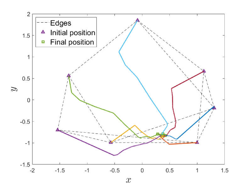
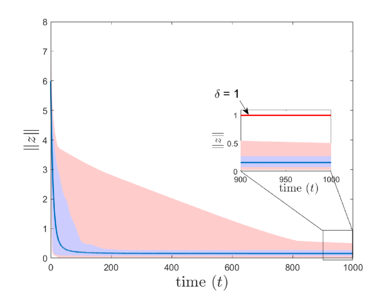
Using the above simulation setup, the results are summarized and presented in Figures 14. The motion animation of both cases can be seen in the following video https://s.id/MAS-NNC. It can be seen from Figure 1 that by using the nearest-neighbor consensus control as proposed in Proposition 1, the agents reach practical consensus as expected. Furthermore, Fig. 2 shows that in the steady-state, the norm of the error vector $z$ is always below 1 for all samples, which confirms the theoretical result in Proposition 1.

Refer to caption
Figure 3: An example of agent trajectories for nearest-neighbor formation control taken from the 1000 random simulations.
Refer to caption
Figure 4: Statistics of the norm of formation error function $e$ with 95% confidence interval (blue area) and 100% data (red area).

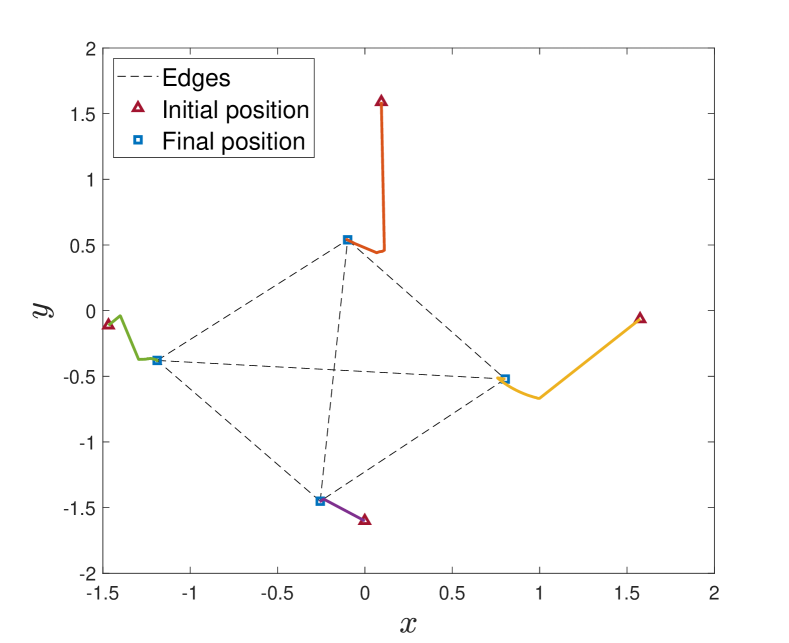
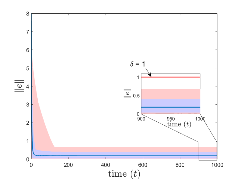
Similar to the consensus case, the nearest-neighbor distance-based formation control as proposed in Proposition 2 also performs as expected. In the formation control case, the desired distances between communicating agents are set so that the positions of all agents are on a circle with the radius of $1$. To show the behaviour of the closed-loop systems using the proposed nearest-neighbor distributed control, a simulation result of a multi-agent system with four agents (taken from the 1000 random simulations) is shown in Fig. 3. In this plot, all agents converge close to the desired formation shape. The statistical plot of Monte Carlo simulations as given in Fig. 4 shows that the norm of the formation error vector converges to a ball that is smaller than the upper bound as computed in Proposition 2. This means that all agents converge close to desired formation shape for all simulations.

Notably, we can observe from the statistical plots in Fig. 2 and Fig. 4 that there should be much tighter bounds to the practical stability results as the bounds obtained from the Monte Carlo simulations is significantly below of the computed bound from Propositions 1 and 2.

V Conclusion

In this letter, we proposed a nearest-neighbor-based input-quantization procedure for multi agent coordination, namely consensus and distance-based formation control problems where agents can only realize finite set of control points. We have provided rigorous analysis for our proposal. Monte Carlo numerical simulations are presented that confirm the practical stability analysis of both consensus and formation control problems.

References

  • [1] L. Moreau, “Stability of continuous-time distributed consensus algorithms,” in 2004 43rd IEEE Conference on Decision and Control (CDC) (IEEE Cat. No.04CH37601), vol. 4, 2004, pp. 3998–4003 Vol.4.
  • [2] W. Ren, R. Beard, and E. Atkins, “A survey of consensus problems in multi-agent coordination,” in Proceedings of the 2005, American Control Conference, 2005., 2005, pp. 1859–1864 vol. 3.
  • [3] L. Li, M. Fu, H. Zhang, and R. Lu, “Consensus control for a network of high order continuous-time agents with communication delays,” Automatica, vol. 89, pp. 144–150, 2018.
  • [4] R. Olfati-Saber, “Flocking for multi-agent dynamic systems: algorithms and theory,” IEEE Transactions on Automatic Control, vol. 51, no. 3, pp. 401–420, 2006.
  • [5] K.-K. Oh, M.-C. Park, and H.-S. Ahn, “A survey of multi-agent formation control,” Automatica, vol. 53, pp. 424–440, 2015.
  • [6] R. Carli and F. Bullo, “Quantized coordination algorithms for rendezvous and deployment,” SIAM Journal on Control and Optimization, vol. 48, no. 3, pp. 1251–1274, 2009.
  • [7] B. S. Park and S. J. Yoo, “Quantized-communication-based neural network control for formation tracking of networked multiple unmanned surface vehicles without velocity information,” Engineering Applications of Artificial Intelligence, vol. 114, p. 105160, 2022.
  • [8] J. Barradas Berglind, H. Meijer, M. van Rooij, S. Clemente Pinol, B. Galvan Garcia, W. Prins, A. Vakis, and B. Jayawardhana, “Energy capture optimization for an adaptive wave energy converter,” in Proceedings of the 2nd International Conference on Renewable Energies Offshore - RENEW 2016.   CRC Press, Taylor and Francis Group, 2016, pp. 171–178.
  • [9] Y. Wei, J. Barradas-Berglind, M. van Rooij, W. Prins, B. Jayawardhana, and A. Vakis, “Investigating the adaptability of the multi-pump multi-piston power take-off system for a novel wave energy converter,” Renewable Energy, vol. 111, pp. 598–610, 2017.
  • [10] M. Marcantoni, B. Jayawardhana, M. P. Chaher, and K. Bunte, “Secure formation control via edge computing enabled by fully homomorphic encryption and mixed uniform-logarithmic quantization,” IEEE Control Systems Letters, vol. 7, pp. 395–400, 2023.
  • [11] Q. Zhang and J.-F. Zhang, “Quantized data–based distributed consensus under directed time-varying communication topology,” SIAM Journal on Control and Optimization, vol. 51, no. 1, pp. 332–352, 2013.
  • [12] C. D. Persis and B. Jayawardhana, “Coordination of passive systems under quantized measurements,” SIAM Journal on Control and Optimization, vol. 50, no. 6, pp. 3155–3177, 2012.
  • [13] M. Jafarian, “Ternary and hybrid controllers for the rendezvous of unicycles,” in 2015 54th IEEE Conference on Decision and Control (CDC), 2015, pp. 2353–2358.
  • [14] J. Wei, X. Yi, H. Sandberg, and K. H. Johansson, “Nonlinear consensus protocols with applications to quantized communication and actuation,” IEEE Transactions on Control of Network Systems, vol. 6, no. 2, pp. 598–608, 2019.
  • [15] J. Cortés, “Finite-time convergent gradient flows with applications to network consensus,” Automatica, vol. 42, no. 11, pp. 1993–2000, 2006.
  • [16] F. Ceragioli and P. Frasca, “Continuous-time consensus dynamics with quantized all-to-all communication,” in 2015 European Control Conference (ECC), 2015, pp. 1926–1931.
  • [17] Z. Sun, H. G. de Marina, B. D. O. Anderson, and M. Cao, “Quantization effects in rigid formation control,” in 2016 Australian Control Conference (AuCC), 2016, pp. 168–173.
  • [18] F. Xiao, T. Chen, and H. Gao, “Consensus in time-delayed multi-agent systems with quantized dwell times,” Systems & Control Letters, vol. 104, pp. 59–65, 2017.
  • [19] B. Jayawardhana, M. Almuzakki, and A. Tanwani, “Practical stabilization of passive nonlinear systems with limited control,” IFAC-PapersOnLine, vol. 52, no. 16, pp. 460–465, 2019, 11th IFAC Symposium on Nonlinear Control Systems NOLCOS 2019.
  • [20] M. Z. Almuzakki, B. Jayawardhana, and A. Tanwani, “Nearest neighbor control for practical stabilization of passive nonlinear systems,” Automatica, vol. 141, p. 110278, 2022.
  • [21] J. P. Hespanha, D. Liberzon, D. Angeli, and E. D. Sontag, “Nonlinear norm-observability notions and stability of switched systems,” IEEE Transactions on Automatic Control, vol. 50, no. 2, pp. 154–168, 2005.
  • [22] C. De Persis, “Robust stabilization of nonlinear systems by quantized and ternary control,” Systems & Control Letters, vol. 58, no. 8, pp. 602–608, 2009.