Spin squeezing in internal bosonic Josephson junctions via enhanced shortcuts to adiabaticity

Abstract

We investigate a time-efficient and robust preparation of spin-squeezed states – a class of states of interest for quantum-enhanced metrology – in internal bosonic Josephson junctions with a time-dependent nonlinear coupling strength between atoms in two different hyperfine states. We treat this state-preparation problem, which had previously been addressed using shortcuts to adiabaticity (STA), using the recently proposed analytical modification of this class of quantum-control protocols that became known as the enhanced STA (eSTA) method. We characterize the state-preparation process by evaluating the time dependence of the coherent spin-squeezing and number-squeezing parameters and the target-state fidelity. We show that the state-preparation times obtained using the eSTA method compare favourably to those found in previously proposed approaches. We also demonstrate that the increased robustness of the eSTA approach – compared to its STA counterpart – leads to additional advantages for potential experimental realizations of strongly spin-squeezed states in bosonic Josephson junctions.

I Introduction

Time-efficient and robust protocols for quantum-state engineering Li+ ; Sto (a); Pen ; Sto (b); Zhe ; Haa (a); Zha (a, b); Erh ; Mac ; Haa (b); Qia ; Fen ; Nau ; Sto (c); Wu+ ; Wan ; Sto (d) represent an important building block of emerging quantum technologies for computing, sensing, and communication Dow . For instance, motivated by their potential quantum-technology applications a multitude of robust schemes for the preparation of highly entangled multiqubit states of $W$ Li+ ; Sto (a); Pen ; Sto (b); Zhe ; Haa (a); Zha (a, b), Greenberger-Horne-Zeilinger (GHZ) Erh ; Mac ; Haa (b); Qia ; Fen ; Nau ; Sto (c), or Dicke Wu+ ; Wan ; Sto (d) type have been proposed in recent years; these schemes are of relevance for diverse physical platforms for quantum information processing. Another interesting class of quantum states are, e.g., large Schrödinger cat states, whose realization was already demonstrated in the past with microwave photons Vla and with mechanical degrees of freedom Leo .

Spin-squeezed states Gro (a) were originally introduced by Kitagawa and Ueda Kit as a means of redistributing the fluctuations of two orthogonal spin directions between each other. Shortly afterwards it was demonstrated that they enable an enhancement in the precision of atom interferometers that measure time, distance, or magnetic fields Wine ; Win – the same feature that had been discovered for photonic squeezed states in optical interferometry a decade earlier Cav . More precisely, they provide phase sensitivities beyond the so-called standard quantum limit $\Delta\theta_{\textrm{SQL}}=1/\sqrt{N}$, which is characteristic of probes that involve a finite number $N$ of uncorrelated or classically correlated particles Gio . The realization that spin-squeezed states allow the possibility to overcome this classical bound, which is inherent to current two-mode atomic sensors Szi , established these states as a useful resource for quantum metrology Pez . Finally, the intimate connection between spin squeezing and entanglement – the ingredient also shared by other types of states that defy the standard quantum limit (e.g. GHZ states) Lee – was subsequently unravelled Sor (a, b). More recent studies of spin squeezing have unravelled interesting connections with seemingly unrelated concepts, such as spontaneous breaking of a continuous symmetry Comp or quantum scrambling Lipp .

The tunability of elastic atom-atom collisions in Bose-Einstein condensates (BECs) allows one to generate a metrologically useful entanglement in these systems Pez ; Fad ; zhang2023 . In particular, the generation of spin-squeezed states was demonstrated in groundbreaking experiments with cold neutral atoms in BECs more than a decade ago Est ; Gro (b); Rie ; Zib . These experimental demonstrations were performed with interacting cold ⁸⁷Rb atoms in bosonic Josephson junctions (BJJs) Gat , a class of systems where bosons within a condensate can be restricted to occupy only two single-atom states (modes). Importantly, these proof-of-principle experiments were carried out both with internal BJJs [those in which two modes correspond to two different internal (hyperfine) atomic states and are linearly coupled] and with external ones (where bosons are trapped in two spatially separated wells of an external double-well potential). More recent experiments with these systems demonstrated more strongly spin-squeezed states than the pioneering ones, in addition to reducing the levels of noise from various sources Ock ; Muessel+:15 .

A specific class of techniques to design control schemes are Shortcuts to Adiabaticity (STA) Chen2010STA ; chen2010b ; ibanez2012 ; torrontegui2013a (for a review, see Ref. STA_RMP:19 ). These are analytical control techniques that mimic adiabatic evolution on much shorter timescales. Analytical control solutions are particularly desirable as they are simpler, provide greater physical insight and allow for additional stability requirements ruschhaupt2012a ; lu2020 . STA have been applied in many different contexts, e.g. li2022 ; kiely2016 ; kiely2018 ; torrontegui2011 . In particular, STA-based proposals for the generation of spin-squeezed states in BJJs were put forward Jul (a, b), along with proposals for engineering other types of entangled states (such as, e.g., NOON states Hat ; Ste ), leading to results comparable to those obtained using optimal control Lap ; Sor (c). However, experimental realizations of these STA-based proposals for quantum-state engineering in BJJs have not been reported to date.

However, STA methods can have limitations as they could require non-trivial physical implementation (e.g. counterdiabatic driving STA_RMP:19 ), while other STA techniques may only be easily applied to small or highly symmetrical systems (e.g. Lewis-Riesenfeld invariants) STA_RMP:19 . This motivated the development of Enhanced Shortcuts to Adiabaticity (eSTA) Whitty+:20 ; Whitty+:22 ; Whitty2022b which allows to correct STA solutions perturbatively and in an analytical way, inspired by optimal-control techniques Werschnik+Gross:07 . The primary motivation behind this new method is the desire to design efficient control protocols for systems to which STA protocols are not directly applicable. More specifically yet, the main idea of eSTA is to first approximate the original Hamiltonian of such a system by a simpler one, tractable within the STA framework. Assuming that the STA protocol for the approximate Hamiltonian is close-to-optimal even when utilized for the treatment of the full system Hamiltonian, the actual eSTA protocol is obtained through a gradient expansion in the control-parameter space. The eSTA method has already proven superior to its STA counterpart in several realistic quantum-control problems pertaining to coherent atom transport in optical lattices Whitty+:20 ; Hau (a, b) and anharmonic trap expansion Whitty2022b . In addition, it was demonstrated that this approach is intrinsically more robust to various sources of imperfections than its STA counterpart Whitty+:22 .

In this paper, motivated by the dearth of experimental realizations of STA-based quantum-state-engineering schemes in BJJs, we revisit the problem of efficiently generating spin-squeezed states in internal BJJs. In order to design a state-preparation scheme that is more amenable to experimental realizations we apply the formalism of eSTA to provide a control scheme with an improved fidelity and an increased robustness to unavoidable imperfections in current cold-atom systems. By making use of the eSTA approach, we determine the time dependence of the interspecies atom-atom interaction strength that allows one to time-efficiently generate spin-squeezed states in an internal BJJ. We quantify the state-preparation process by evaluating the time dependence of the target-state fidelity, as well as that of the coherent spin-squeezing and number-squeezing parameters. In this manner, we show that spin-squeezed states can be engineered in BJJs within times significantly shorter than those in the existing experimental realizations of such states Est ; Gro (b); Rie . We also demonstrate that our eSTA-based control scheme yields better results than its STA counterpart, both in terms of achievable squeezing and robustness to various types of systematic errors, most prominently a systematic control-amplitude error.

The remainder of the present paper is organized as follows. In Sec. II, after briefly reviewing the physics of an internal BJJ, we introduce its governing Bose-Hubbard-type Hamiltonian, recasting in the Lipkin-Meshkov-Glick form. We then invoke the well-known mapping of the two-site (or two-state) Bose-Hubbard model of a BJJ to a fictitious particle in a nearly harmonic potential, which is described by a single-particle Schrödinger-like equation in Fock space. Finally, we also introduce some figures of merit for characterizing spin squeezing. In Sec. III we apply the eSTA formalism to the system under consideration. The squeezed-state fidelities computed within the proposed eSTA-based control scheme are then presented and discussed in Sec. IV, where we also demonstrate the extraordinary robustness of our proposed, eSTA state-preparation scheme. We summarize the paper, with some concluding remarks and outlook, in Sec. V.

II System and spin-squeezed states

II.1 Internal BJJs and their underlying many-body Hamiltonian

Internal BJJs are created with trapped BECs in two different internal (hyperfine) states Ste , e.g. a condensate of ⁸⁷Rb atoms in the $|F=1,m_{\textrm{F}}=1\rangle$ and $|F=2,m_{\textrm{F}}=-1\rangle$ hyperfine levels of the electronic ground state of rubidium. Such a system is typically prepared in practice by trapping the atoms in the two internal states in the wells of a deep one-dimensional optical lattice; the lattice depth should be sufficiently large that there is no tunnelling coupling between different wells Gro (b). The Josephson-like coupling in those systems is enabled by an electromagnetic field that coherently transfers particles between the two relevant internal states – to be denoted in what follows by $|\psi_{1}\rangle$ and $|\psi_{2}\rangle$ – via Rabi rotations Hal . Under the assumption that the external motion of the atoms in such a system is not influenced by internal dynamics, it is permissible to use a single-mode approximation for each atomic species (i.e., each hyperfine state). A pictorial illustration of an internal BJJ is provided in Fig. 1.

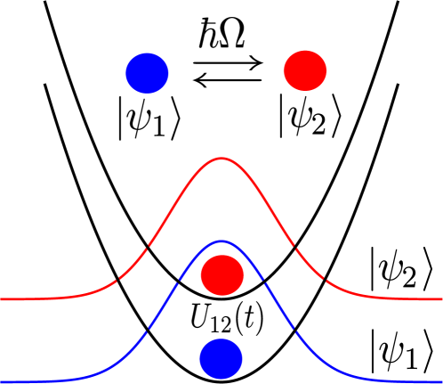
Figure 1: Pictorial illustration of an internal BJJ: An external electromagnetic field coherently transfers atoms between the two relevant hyperfine states (modes), denoted by $|\psi_{1}\rangle$ and $|\psi_{2}\rangle$, via Rabi rotations; $\hbar\Omega$ is the corresponding constant Rabi-coupling strength. The interspecies interaction strength $U_{12}(t)$, which is assumed to be time-dependent, can be varied using an external magnetic field in the presence of a Feshbach resonance.

The many-body Hamiltonian of an internal BJJ is given by that of a two-state Bose-Hubbard model, which using the Schwinger-boson formalism can be recast in the form that represents a special case of the Lipkin-Meshkov-Glick family of Hamiltonians Lip :

$$H_{\textrm{IBJJ}}(t)=U(t)J_{z}^{2}-\hbar\Omega J_{x}\>.$$ (1)

Here $\hbar\Omega$ is the (constant) strength of Josephson-like (Rabi) coupling and $U(t)$ is the nonlinear coupling (i.e. two-body interaction) strength, which we assume to be time-dependent in what follows (we also assume repulsive interactions, hence $U(t)>0$, at initial and final time); $\mathbf{J}\equiv\{J_{x},J_{y},J_{z}\}$ are pseudoangular-momentum (collective spin) operators, given in terms of the boson creation and annihilation operators corresponding to the two modes ($a^{\dagger}_{i}$ and $a_{i}$, respectively, where $i=1,2$) as

$$J_{x} = \frac{1}{2}\>(a^{\dagger}_{1}a_{2}+a^{\dagger}_{2}a_{1})\>,$$

$$J_{y} = \frac{1}{2i}\>(a^{\dagger}_{1}a_{2}-a^{\dagger}_{2}a_{1})\>,$$ (2)

$$J_{z} = \frac{1}{2}\>(a^{\dagger}_{1}a_{1}-a^{\dagger}_{2}a_{2})\>.$$

Thus, the Hamiltonian of the system at hand is given by the sum of the one-axis twisting term $U(t)J_{z}^{2}$ and the Josephson (Rabi-coupling) term $-\hbar\Omega J_{x}$. The dimensionless parameter $\Lambda\equiv NU/(\hbar\Omega)$ quantifies the relative importance of interactions and Rabi coupling in an internal BJJ Gro (a). In particular, in the problem at hand where $U=U(t)$ is assumed to depend on time, the parameter $\Lambda$ will also be time-dependent.

The Rabi-coupling parameter $\hbar\Omega$ and interaction strength $U$ in the Hamiltonian of Eq. (1) are given by

$$\Omega = \Omega_{R}\int d^{3}\mathbf{r}\>\psi^{*}_{1}(\mathbf{r})\psi_{2}(\mathbf{r})\>,$$

$$U = U_{11}+U_{22}-2U_{12}\>,$$ (3)

$$U_{ij} = \frac{2\pi\hbar^{2}a^{(i,j)}_{s}}{M}\int d^{3}\mathbf{r}|\psi_{i}(\mathbf{r})|^{2}|\psi_{j}(\mathbf{r})|^{2}\>,$$

where $\Omega_{R}$ is the Rabi frequency, $a^{(i,j)}_{s}$ ($i,j=1,2$) are intraspecies ($i=j$) and interspecies ($i\neq j$) $s$-wave scattering lengths, and $\psi_{1,2}(\mathbf{r})\equiv\langle\mathbf{r}|\psi_{1,2}\rangle$ are mode functions of the two internal states. In particular, the interspecies $s$-wave scattering length $a^{(1,2)}_{s}$ for ⁸⁷Rb atoms in internal BJJs can be varied using an external magnetic field owing to the presence of Feshbach resonance Zib ; in practice, this mechanism is used to reduce the interspecies $s$-wave scattering length, because for ⁸⁷Rb atoms there is a nearly perfect compensation of intraspecies and interspecies interactions. In this manner one can externally control the time dependence $U(t)$ of the nonlinear coupling parameter [cf. Eq. (1)]. An alternative approach for tuning the nonlinear coupling strength entails controlling the wave-function overlap between the two relevant internal states in a state-dependent microwave potential Rie ; this approach also works in magnetic traps and for pairs of internal atomic states for which no convenient Feshbach resonances exist.

The control task that we will be concerned with in the remainder of this work amounts to designing a control function $U(t)$ [or, equivalently, the time dependence of the dimensionless parameter $\Lambda(t)$] such that we start at $t=0$ in the ground state of the Hamiltonian $H_{\textrm{IBJJ}}$ [cf. Eq. (1)] with a given $U(t=0)\equiv U_{0}=0$ (coherent spin state with equal atomic populations in the two relevant internal states) and end up at $t=t_{f}$ in the ground state of that Hamiltonian with a different given $U(t=t_{f})\equiv U_{f}$ (the desired spin-squeezed state). While this is not generically the case in control problems treated using the STA- and eSTA methods STA_RMP:19 , both the initial and final states in our envisioned scheme for the preparation of spin-squeezed states correspond to ground states of the Hamiltonian of the system. This obviates the need for stopping or freezing the system dynamics once the desired spin-squeezed state is generated, a feature that makes our state-preparation scheme more flexible and robust.

II.2 Mapping to a Schrödinger-like equation in Fock space

In the following, we will review the well-known mapping of the two-site (or two-state) Bose-Hubbard model of a BJJ to a fictitious particle in a nearly harmonic potential, which is described by a single-particle Schrödinger-like equation in Fock space Mah ; Shc .

The time-dependent Schrödinger equation of this system is written as

$$i\hbar\frac{\partial}{\partial t}\ket{\Psi}=H_{\textrm{IBJJ}}\ket{\Psi}\>.$$ (4)

By making use of the pseudoangular momentum approach [cf. Sec. II.1], a system of $N$ particles can be described as a single particle with spin $N/2$ and the basis set is of the form $\{\ket{m}\}$, with $m=-N/2,...,N/2$ being the eigenvalues of the operator $J_{z}$. The general state $\ket{\Psi}$ can be written as

$$\ket{\Psi}=\sum_{m=-N/2}^{N/2}c_{m}\ket{m}\>,$$ (5)

with $\sum_{m=-N/2}^{N/2}\left|c_{m}\right|^{2}=1$ and $\innerproduct{m}{m^{\prime}}=\delta_{m,m^{\prime}}$. By making use of Eqs. (4) and (5), we readily obtain

$$i\hbar\frac{d}{dt}c_{m}(t)$$

$$= -\frac{\hbar\Omega}{2}\left[\beta_{m}c_{m+1}(t)+\beta_{m-1}c_{m-1}(t)\right]+U(t)m^{2}c_{m}(t)\>,$$

where

$$\beta_{m} = \langle m|J_{-}|m+1\rangle=\langle m+1|J_{+}|m\rangle$$ (7)

$$= \sqrt{\left(\frac{N}{2}+m+1\right)\left(\frac{N}{2}-m\right)}.$$

This result yields a Schrödinger equation for the coefficients $c_{m}(t)$, where $m=-N/2,-N/2+1,...N/2$. Note that Eq. (LABEL:eq:numerical) [resp. the equivalent Eq. (4)] will also be used for the numerically exact simulation of the system at hand in this work.

We now proceed to rewrite this discrete formulation of Eq. (LABEL:eq:numerical) as a continuous one by performing a change of variables. To this end, we define $h=\frac{1}{N/2}$ and $z_{m}=\frac{m}{N/2}$ (the relative population difference between the two relevant hyperfine states); we then find that $z_{m\pm 1}=z_{m}\pm h$ and $-1\leq z_{m}\leq 1$. By also defining

$$b_{h}(z_{m})=\frac{\beta_{m}}{N}=\frac{1}{2}\sqrt{\left(1+z_{m}+h\right)\left(1-z_{m}\right)}\>,$$ (8)

we obtain that $\beta_{m-1}/N=\frac{1}{2}\sqrt{\left(1+z_{m}\right)\left(1-z_{m}-h\right)}=b_{h}(z_{m}-h)$. Additionally, we introduce $\psi(t,z_{m})=\sqrt{N/2}\>c_{m}(t)$ and straightforwardly verify that $\psi(t,z_{m}\pm h)=\sqrt{N/2}\>c_{m\pm 1}(t)$. In addition, we have that $\sum_{m=-N/2}^{N/2}h\left|\psi(t,z_{m})\right|^{2}=1$, because $\sum_{m=-N/2}^{N/2}\left|c_{m}(t)\right|^{2}=1$.

At this point we can switch to the continuum approximation for the relative population difference ($z_{m}\rightarrow z$), introducing at the same time a dimensionless time $\tau$, such that $t=2\tau/\Omega$. In this manner, we can finally recast Eq. (LABEL:eq:numerical) in the form

$$ih\partial_{\tau}\psi(\tau,z)$$ (9)

$$= -2\left[b_{h}(z-h)\psi(\tau,z-h)+b_{h}(z)\psi(\tau,z+h)\right]$$

$$+\Lambda(\tau)z^{2}\psi(\tau,z)\>.$$

Let us set $b_{h}(z)=0$ for all $z\leq-1-h$ and $z\geq 1$, as well as $\psi(t,z)=0$ all $z\leq-1-h$ and $z\geq 1+h$. It is worthwhile to note that if this equation is fulfilled for $z\in[-1-h,1+h]$ (it will be trivially fulfilled outside this interval) then it is obviously also fulfilled for all $z_{m}$ ($m=-N/2,...N/2$) in the discrete description; therefore, Eq. (9) is equivalent – in the continuum approximation – to Eqs. (4) and (LABEL:eq:numerical).

Equation (9) will be one of our starting points in the following for constructing the control schemes using the eSTA formalism. This equation is often rewritten further by recalling that for a differentiable function $f(x)$ it holds that $f(x\pm\epsilon)=e^{\pm\epsilon\partial_{x}}f(x)$. As a result, we arrive at the equation $ih\partial_{\tau}\psi(\tau,z)=H_{2}\psi(\tau,z)$, where

$$H_{2} = -2\left[e^{-ip}b_{h}(z)+b_{h}(z)e^{ip}\right]$$ (10)

$$+\Lambda(\tau)z^{2}$$

and $p=-ih\partial_{z}$.

We now want to derive an approximated version of Eq. (10). By performing a Taylor expansion of both the $e^{\pm ip}$ part and the function $b_{h}(z)$ up to the second order in $h$, we obtain

$$e^{\pm ip} = e^{\pm h\partial_{z}}\approx 1\pm h\partial_{z}-\frac{1}{2}h^{2}\partial^{2}_{z}\>,$$ (11)

$$b_{h}(z) \approx 1+h\partial_{h}b_{h}(z)|_{h=0}+\frac{1}{2}h^{2}\partial_{h}^{2}b_{h}(z)|_{h=0}\>.$$ (12)

For a small $h$, neglecting a constant energy shift, we get approximately the Hamiltonian Shc

$$H_{1}=-h^{2}\partial_{z}b_{0}(z)\partial_{z}+\Lambda(\tau)z^{2}-2b_{0}(z)\>,$$ (13)

where $b_{0}(z)=\sqrt{1-z^{2}}$. In the following, the Hamiltonian in Eq. (13) will serve as a second, alternative starting point for constructing the control schemes using the eSTA formalism.

If we assume, in addition, that $z$ is small (i.e. the population difference between the two states is small compared to the total particle number $N$) and neglect a constant energy shift, we obtain the Hamiltonian of a harmonic oscillator

$$H_{0}=-h^{2}\partial^{2}_{z}+\left[\Lambda(\tau)+1\right]z^{2}\>.$$ (14)

Note that this last Hamiltonian has been the starting point for deriving the STA scheme in Ref. Jul (a). In the following, we will use it as our primary point of departure for developing an eSTA-type control scheme.

The control task that we will address in the following now reduces to finding a control function $\Lambda(t)$ such that we start at $\tau=0$ in the ground state of the Hamiltonian (1) with a given $\Lambda(0)=\Lambda_{i}$ [resp. $U(0)=\hbar\Omega\Lambda_{i}/N=U_{0}$] and we end at $\tau=\tau_{f}$ in the ground state of the Hamiltonian (1) with a different given $\Lambda(\tau_{f})=\Lambda_{f}$ [resp. $U(\tau_{f})=\hbar\Omega\Lambda_{f}/N=U_{f}$].

II.3 Squeezing parameters

Given that in the remainder of this work we will be concerned with spin-squeezed states, it is pertinent to introduce at this point the relevant figures of merit of spin squeezing. In particular, two such quantities are the number-squeezing- and coherent spin-squeezing parameters. We define them in what follows adopting the standard convention according to which the mean collective spin points in the direction of $J_{x}$ and the direction of minimal variance is that of $J_{z}$ [cf. Eq. (2)]. The length of the collective spin will be denoted by $J\equiv N/2$.

The number-squeezing parameter, which in the problem at hand depends on time, is defined in terms of expectation values of the collective spin operators as Wine

$$\xi^{2}_{N}(t)=\frac{2}{J}\>\Delta J^{2}_{z}=\frac{\Delta J^{2}_{z}}{N/4}\>,$$ (15)

where $\Delta J^{2}_{z}\equiv\langle J^{2}_{z}\rangle-\langle J_{z}\rangle^{2}$ is the variance of the operator $J_{z}$. Here $J/2=N/4$ corresponds to the shot-noise limit, i.e. to the coherent spin state with $\langle J_{z}\rangle=0$. Therefore, a many-body state is number-squeezed ($\xi_{N}<1$) if the variance of one spin component is smaller than the shot-noise limit.

The (time-dependent) coherent spin-squeezing parameter is defined as Sor (a)

$$\xi^{2}_{S}(t)=\frac{N\Delta J^{2}_{z}}{\langle J_{x}\rangle^{2}}=\frac{\xi^{2}_{N}(t)}{\alpha^{2}(t)}\>,$$ (16)

where $\alpha(t)\equiv\langle\Psi(t)|2J_{x}/N|\Psi(t)\rangle$ is the measure of the phase coherence of the many-body state $|\Psi(t)\rangle$. The parameter $\xi_{S}$ quantifies the complex interplay between an improvement in number squeezing and loss of coherence. Importantly, this parameter can be used to quantify precision gain in interferometry; namely, the interferometric precision is increased to $\Delta\theta=\xi_{S}/\sqrt{N}$ (compared to the standard quantum limit $1/\sqrt{N}$) for spin-squeezed states Gro (a). Moreover, the inequality $\xi^{2}_{S}<1$ signifies that the many-body state in question is entangled Sor (a).

III Application of eSTA formalism

The general formalism of eSTA was derived in Whitty+:20 ; Whitty+:22 ; Whitty2022b . Its starting point is the exact system Hamiltonian $H_{S}$. This Hamiltonian can be approximated by a Hamiltonian $H_{0}$, where a control function $\Lambda_{0}(t)$ can be derived for $H_{0}$ using STA techniques; this control function $\Lambda_{0}(t)$ results in a fidelity equal to one for $H_{0}$. However, when this control scheme is applied to the exact system Hamiltonian $H_{S}$, the fidelity will in general obviously be lower than one. However, by making use of the eSTA formalism, we can then calculate analytically an improved control scheme $\Lambda(t)=\Lambda_{0}(t)+P_{\vec{\lambda}}(t)$ based on the knowledge of the STA control scheme for $H_{0}$ that results in a larger fidelity when applied to the exact system Hamiltonian $H_{S}$ (see below for the definition of $P_{\vec{\lambda}}(t)$ and more details).

In what follows, we apply the general eSTA framework to the preparation of spin-squeezed states in internal BJJs. We will consider two different approaches in the following. In the first, simplified approach, we assume that the system Hamiltonian is given by the approximated Hamiltonian $H_{S,1}=H_{1}$ given by Eq. (13). This Hamiltonian can be approximated by $H_{0}$ given by Eq. (14) and an STA control scheme $\Lambda_{0}$ has been derived for this Hamiltonian in Ref. Jul (a). This will be the first starting point for applying the general formalism of eSTA in the problem at hand.

In the second approach, we assume that the system Hamiltonian is given by the exact Hamiltonian $H_{S,2}=H_{2}$ of Eq. (10), which is equivalent to $H_{\textrm{IBJJ}}$. This Hamiltonian can again be approximated by $H_{0}$ given by Eq. (14). This will be the second starting point for applying the general formalism of eSTA in this work.

In the problem under consideration, the approximated Hamiltonian $H_{0}$ is given by Eq. (14). In Sec. III.1 below, we first briefly review how an STA control scheme, characterized by the control function $\Lambda_{0}(\tau)$, was designed in Ref. Jul (a) for the same Hamiltonian. Their resulting control function $\Lambda_{0}(\tau)$ will be the basis for developing the enhanced STA scheme in the present work.

III.1 Review of STA scheme for harmonic approximation $H_{0}$

The case of a time-dependent $U(t)$ and a constant $\hbar\Omega$ based on the harmonic approximation was investigated in Ref. Jul (a), whose main result are summarized in what follows.

Derived using Lewis-Riesenfeld invariants, we show that the following wave function fulfills the time-dependent Schrödinger equation for the harmonic oscillator Hamiltonian $H_{0}$ [see Eq. (14)]

$$\chi_{n}(t,z)=$$ (17)

$$\left(\frac{1}{\pi z_{0}^{2}}\right)^{1/4}\frac{1}{\sqrt{2^{n}!b(t)^{2}}}\>{\displaystyle e^{i\varphi(t)-\frac{z^{2}}{2z_{0}^{2}b(t)^{2}}+i\frac{b^{\prime}(t)\tau}{4hb(t)}}}$$

$$\times H_{n}\left[\left(\frac{z}{z_{0}b(t)}\right)\right]\>,$$

where the auxiliary function $b(t)$ must be a solution of the Ermakov equation

$$b^{\prime\prime}(t)-\frac{\omega_{0}^{2}}{b(t)^{3}}+b(t)\omega(t)^{2}=0\>.$$

We have here also $\varphi(t)=-\int_{0}^{t}ds\,\frac{h(1+2n)}{\tau z_{0}^{2}b(t)^{2}}$, $\omega(t)^{2}=\frac{4(1+\Lambda(t))}{\tau^{2}}$ and $z_{0}=\sqrt{2h/(\tau\omega(0))}$ and $\omega_{0}=\omega(0)$. We now use inverse engineering by first fixing a function $b(t)$ that satisfies the boundary conditions $b(0)=1$, $b(t_{f})=\gamma$, $b^{\prime}(0)=b^{\prime}(t_{f})=b^{\prime\prime}(0)=b^{\prime\prime}(t_{f})=0$, where $\gamma=\sqrt{\omega(0)/\omega(t_{f})}$. In the following, we will choose a polynomial of degree $6$ that satisfies these conditions. By inverting the above equation, we obtain an explicit expression for the required physical control function $\Lambda(t)$ resp. $U(t)$:

$$\Lambda_{0}(t)=\frac{U(t)N}{\hbar\Omega}=-1+\frac{\Lambda(0)}{b(t)^{4}}-\frac{\tau^{2}b^{\prime\prime}(t)}{4b(t)}\>.$$ (18)

III.2 eSTA correction of the control function

As mentioned above, the key idea of enhanced STA is to modify the STA control function by taking into account that the approximated Hamiltonian $H_{0}$ – which is amenable to STA treatment – is different from the exact system Hamiltonian $H_{S}$. We assume that the modified control function is $\Lambda(t)=\Lambda_{0}(t)+P_{\vec{\lambda}}(t)$. We consider here a polynomial $P_{\vec{\lambda}}(t)$ of degree $\nu+2$ ($\nu$ being a positive integer) that would take some values $\vec{\lambda}=(\lambda_{0},...,\lambda_{\nu+1})$ in the interval for some $t\in[t_{0},t_{\nu+1}]$ with $\lambda_{0}=\lambda_{\nu+1}=0$, and $t_{0}=t_{0},t_{\nu+1}=t_{f}$, i.e. $P_{\vec{\lambda}}(t_{j})=\lambda_{j}$. It is helpful to use the Lagrange interpolation that would take the form

$$P_{\vec{\lambda}}(t)=\sum_{j=0}^{\nu+1}\lambda_{j}\prod_{\begin{subarray}{c}k=0\\ k\neq j\end{subarray}}^{\nu+1}\frac{t-t_{k}}{t_{j}-t_{k}}\>.$$ (19)

The expression for $P_{\vec{\lambda}}(t)$ can be simplified even further by demanding that $\lambda_{0}=\lambda_{\nu+1}=0$:

$$P_{\vec{\lambda}}(t)=\sum_{j=1}^{\nu}\lambda_{j}\prod_{\begin{subarray}{c}k=1\\ k\neq j\end{subarray}}^{\nu}\frac{t-t_{k}}{t_{j}-t_{k}}\>.$$ (20)

These corrections $\vec{\lambda}$ are calculated by making approximation about the value of the fidelity landscape. We start by defining the auxiliary functions $G_{n}$, $K_{n}$ and $\mathrm{H}$ that will later be used to calculate $\vec{\lambda}$ Whitty+:20 ; Whitty2022b . Let $\Delta H=H_{S}-H_{0}$ be the difference between the exact system Hamiltonian and the approximated one. Using the STA wave functions $\chi_{n}$ of the approximated Hamiltonian [cf. Eq. (17)] we can evaluate $G_{n}$ using the formula

$$G_{n}=\int_{0}^{t_{f}}dt\innerproduct{\chi_{n}}{\Delta H|\chi_{0}}\>.$$ (21)

Similarly, we can calculate $\vec{K}_{n}$ as

$$\vec{K}_{n}=\int_{0}^{t_{f}}dt\innerproduct{\chi_{m}}{\vec{\nabla}H_{S}|\chi_{0}}\>,$$ (22)

where $\vec{\nabla}H_{S}$ is the gradient of the Hamiltonian with respect to the control parameter $\vec{\lambda}$. In addition, let us define the Hessian matrix $\mathcal{H}$ with matrix elements

$$\mathcal{H}_{l,k}=\sum_{n=1}^{\mathcal{N}}\left[G_{n}(W_{n})_{l,k}+\left(\vec{K}^{*}_{n}\right)_{k}\left(\vec{K}_{n}\right)_{l}\right]\>,$$ (23)

where $(W_{n})_{l,k}=\innerproduct{\chi_{n}}{\partial_{\lambda_{l}}\partial_{\lambda_{k}}H_{S}|\chi_{0}}$ is a matrix evaluated by taking the second derivative with respect to the control parameter and $\mathcal{N}$ is the number of STA wave functions that we take into account.

We can now calculate the correction parameters $\vec{\lambda}$ using $G_{n}$ and $K_{n}$, assuming that a fidelity equal to unity can be achieved for the exact Hamiltonian Whitty+:20 . Alternatively, the correction parameters $\vec{\lambda}$ can be computed using $G_{n}$, $K_{n}$, and the values of $\mathcal{H}_{l,k}$ Whitty2022b . We will follow the second procedure and the correction parameters $\vec{\lambda}$ can be calculated via

$$\vec{\lambda}=\frac{\vec{v}\norm{v}^{2}}{\vec{v}^{T}\mathrm{H}\vec{v}}\>,$$ (24)

where

$$\vec{v}=\sum_{n=1}^{\mathcal{N}}\text{Re}(G_{n}^{*}\vec{K}_{n})\>.$$ (25)

In the first eSTA-based approach, we choose $H_{S,1}=H_{1}$, as already mentioned above. In this case we have

$$\Delta H_{1}=-h^{2}\partial_{z}b_{0}(z)\partial_{z}+h^{2}\partial^{2}_{z}-2b_{0}(z)-z^{2}\>,$$ (26)

where we can see that the control function $\Lambda(t)$ is cancelled out here. Recalling the form of $H_{1}$ [cf. Eq. (13)], we can see that the only part that depends on $\lambda_{i}$ is the $z^{2}$ term. Now taking the gradient of $H_{1}$ with respect to the control parameters in this case only amounts to performing the following derivatives

$$\partial_{\lambda_{i}}H_{S,1}=\partial_{\lambda_{i}}H_{1}=\partial_{\lambda_{i}}\tilde{\Lambda}(\tau)z^{2}$$ (27)

$$= \partial_{\lambda_{i}}\left[\Lambda_{0}z^{2}+P_{\vec{\lambda}}(t)z^{2}\right]=z^{2}\prod_{\begin{subarray}{c}k=2\\ k\neq i\end{subarray}}^{n-1}\frac{t-t_{k}}{t_{i}-t_{k}}\>.$$

This results in

$$\Braket{\chi_{m}}{\partial_{\lambda_{i}}H_{S_{1}}}{\chi_{0}}=\prod_{\begin{subarray}{c}k=2\\ k\neq i\end{subarray}}^{n-1}\frac{t-t_{k}}{t_{i}-t_{k}}\Braket{\chi_{m}}{z^{2}}{\chi_{0}}\>.$$ (28)

Due to the symmetry and properties of $\chi_{n}$, it follows that this expression has a nonzero value only for $m=2$ and, therefore, only $\vec{K}_{2}$ is nonzero in this case. Because $\Lambda$ is only linear in $\vec{\lambda}$, it also follows that $W_{n}=0$. In this way Eqs. (25) and (23) simplify significantly, and we can write

$$\vec{v}=\text{Re}(G_{2}^{*}\vec{K}_{2})$$ (29)

$$\mathcal{H}_{l,k}=\left(\vec{K}^{*}_{2}\right)_{k}\left(\vec{K}_{2}\right)_{l}\>.$$ (30)

The correction parameters $\vec{\lambda}_{1}$ in this approach are then given by Eq. (24). In the following, we set $\nu=5$ and denote the resulting control function by $\Lambda_{1}$.

In the second eSTA-based approach, we choose $H_{S,2}=H_{2}$ as already mentioned above. In this case we have

$$\Delta H_{2}=-2\left[e^{-ip}b_{h}(z)+b_{h}(z)e^{ip}\right]+h^{2}\partial^{2}_{z}-z^{2}\>,$$ (31)

where we can see that the control function $\Lambda(t)$ is again cancelled out here. The form of $H_{2}$ [cf. Eq. (10)] implies that again the only part dependent on $\lambda_{i}$ is the $z^{2}$ term. Therefore, similar to the above case we obtain

$$\Braket{\chi_{m}}{\partial_{\lambda_{i}}H_{S_{2}}}{\chi_{0}}=\prod_{\begin{subarray}{c}k=2\\ k\neq i\end{subarray}}^{n-1}\frac{t-t_{k}}{t_{i}-t_{k}}\Braket{\chi_{m}}{z^{2}}{\chi_{0}}\>,$$ (32)

which is nonzero only for $m=2$, resulting in similar expressions as Eq. (30), however with a different value of $G_{2}$. The corresponding correction parameters $\vec{\lambda}_{2}$ in the second approach are then again given by Eq. (24). In the following, we consider the cases of $\nu=5$ (the resulting control function will be denoted $\Lambda_{2}$) and $\nu=1$ (the control function denoted by $\widetilde{\Lambda}_{2}$). In the following section we will examine these three resulting control schemes based on the eSTA formalism.

IV Results and discussion

In this section, we apply the eSTA scheme – as described in the previous section – to a BJJ. We apply the eSTA protocol to both the Hamiltonian $H_{1}$ and $H_{2}$ with $\nu=5$ corrections (control functions $\Lambda_{1}$ and $\Lambda_{2}$), as well as applying the protocol to $H_{2}$ with $\nu=1$ corrections (control function $\widetilde{\Lambda}_{2}$).

We will compare the results of different eSTA schemes between each other and with the results obtained using the original STA scheme $\Lambda_{0}$, as well as with the results of an adiabatic control scheme $\Lambda_{ad}(t)$. The adiabatic scheme is a polynomial of degree $3$ determined by the conditions $\Lambda_{ad}(0)=\Lambda_{i}$, $\Lambda_{ad}(t_{f})=\Lambda_{f}$, $\Lambda^{\prime}_{ad}(0)=\Lambda^{\prime}_{ad}(t_{f})=0$. For better comparison with previous works, we introduce the Rabi time $t_{R}=2\pi/\Omega$ and use it as the characteristic timescale in the problem at hand; in other words, the squeezed-state preparation times in the following will be expressed in units of $t_{R}$.

Given that we have adopted the Rabi time $t_{R}$ as the characteristic timescale in the problem under consideration, it is of interest to consider relevant values of $t_{R}$ in the experimental realizations of internal BJJs. It is pertinent to do so using as a guide two of the first experiments demonstrating spin squeezing in these systems Gro (b); Rie . In particular, a Rabi coupling with the parameter $\Omega$ in the range from $0$ to $2\pi\times 600$ Hz was implemented in Gro (b), while $\Omega=2\pi\times 10$ Hz was used in Rie . Assuming values of $\Omega$ in the same range as in these experiments, for $\Omega=2\pi\times 2$ Hz we obtain the Rabi time $t_{R}=500$ ms, while for $\Omega=2\pi\times 10$ Hz we find $t_{R}=2\pi/\Omega=100$ ms.

IV.1 Target-state fidelity in different control schemes

We will first discuss the target-state fidelity defined as $F=\left|\langle\Psi_{T}|\Psi(t_{f})\rangle\right|^{2}$, where $\Psi_{T}$ is the target state, i.e. the ground state of the Hamiltonian $H_{\textrm{IBJJ}}$ in Eq. (1) for $t=t_{f}$, while $\ket{\Psi(t_{f})}$ is the state obtained by the time evolution of the system driven by the Hamiltonian $H_{\textrm{IBJJ}}$ (1) with the control scheme $\Lambda(t)$ applied. We will consider the special case with $\Lambda(0)=0$ and $\Lambda(t_{f})=50$ in the following.

An example of this can be found in Fig. 2, where the time evolution of different features can be seen. In this case we considered a system with $N=10$ particles and the evolution runs from $t=0$ to $t_{f}=0.1\,t_{R}$. In Fig. 2(a) we can see the different control functions $\Lambda(t)$ as function of time for the different approaches, respectively adiabatic $\Lambda_{ad}$, STA scheme $\Lambda_{0}$ and the eSTA scheme $\Lambda_{2}$ (applied to $H_{2}$ with $\nu=5$).

The remaining figures are the time evolution of the number squeezing $\xi_{N}^{2}$ of Eq. (15) [Fig. 2(b)] and the coherent spin-squeezing parameter $\xi_{S}^{2}$ of Eq. (16) expressed in dB [Fig. 2(c)], as well as the fidelity $F$ [Fig. 2(d)] when the three different control functions are applied. We can already see that the eSTA scheme $\Lambda_{2}$ gives rise to a higher fidelity than the STA scheme $\Lambda_{0}$, without compromising the achievable squeezing. To examine this in more detail, we plot the fidelity for different final times $t_{f}$ and for different eSTA protocols ($\Lambda_{1},\Lambda_{2},\widetilde{\Lambda}_{2}$). The results are summarized in Fig. 3, for $N=10$ and $N=100$ particles. We can clearly see that eSTA outperforms its STA counterpart even when only one correction (control function $\widetilde{\Lambda}_{2}$) is used, or when it is applied to an approximated version of the original Hamiltonian of the system (control function $\Lambda_{1}$). The effect is more pronounced for smaller particle numbers as the approximation of $H_{\textrm{IBJJ}}$ with $H_{0}$ tends to lose its validity, thus increasing the effects inherent to the eSTA approach.

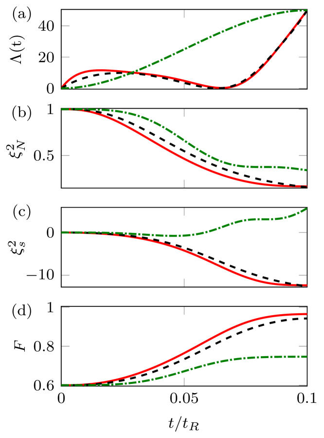
Figure 2: Time evolution of (a) control function $\Lambda(t)$, (b) number squeezing $\xi_{N}^{2}(t)$, (c) coherent spin squeezing $\xi_{S}^{2}(t)$ in dB, (d) fidelity $F(t)$. Enhanced STA applied to discrete Hamiltonian (control function $\Lambda_{2}$, $\nu=5$: red, solid lines), STA (control function $\Lambda_{0}$, black, dashed lines), reference adiabatic scheme (control function $\Lambda_{ad}$, green, dashed-dotted lines). $N=10$, $t_{f}=0.1t_{R}$, $\Lambda(0)=0$, $\Lambda(t_{f})=50$.

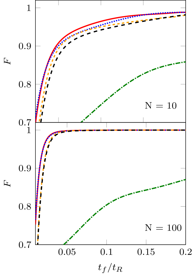
Figure 3: Fidelities $F$ versus final time $t_{f}$ for eSTA applied to Hamiltonian $H_{2}$ ($\Lambda_{2}$, $\nu=5$: red, solid lines; $\widetilde{\Lambda}_{2}$, $\nu=1$: blue, dotted lines), eSTA applied to approximated Hamiltonian $H_{1}$ ($\Lambda_{1}$, orange,small dashed line), STA scheme ($\Lambda_{0}$, black, dashed lines) and as a reference adiabatic scheme ($\Lambda_{ad}$, green, dashed-dotted lines) with different particle numbers $N=10$ (above), $N=100$ (below). $\Lambda(0)=0$, $\Lambda(t_{f})=50$.

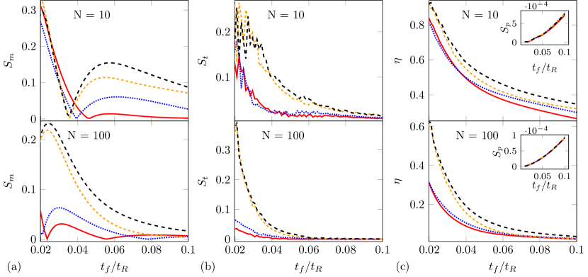
Figure 4: (a) Sensitivity $S_{m}$ for systematic amplitude error, (b) sensitivity $S_{t}$ for systematic time-shift, (c) imperfection $\eta$; inset: sensitivity $S_{p}$ for phase noise. eSTA applied to Hamiltonian $H_{2}$ ($\Lambda_{2}$, $\nu=5$: red, solid lines; $\widetilde{\Lambda}_{2}$, $\nu=1$: blue, dotted lines), eSTA applied to approximated Hamiltonian $H_{1}$ ($\Lambda_{1}$, orange, small dashed line), STA scheme ($\Lambda_{0}$, black, dashed lines).Different particle numbers: $N=10$ (above), $N=100$ (below). The best result is obtained for $\Lambda_{2}$, $\nu=5$ corrections and eSTA applied to the original Hamiltonian (solid red line) as it ensures lowest sensitivity to systematic errors and highest fidelity.

IV.2 Stability of the control schemes

An important property of the control schemes is their robustness. Therefore, in the following, we will consider systematic errors, i.e. an unknown, constant error in the experimental setup. First, we consider a systematic error in the amplitude of the control function $\Lambda(t)$ of the form $\Lambda_{\delta,m}=(1+\delta)\Lambda(t)$ for $t\in[0,t_{f}]$ and for an unknown constant value of $\delta$. We calculate numerically the systematic error sensitivity of the control scheme:

$$S_{m}=\left|\frac{\partial F}{\partial\delta}\right|_{\delta=0}\>.$$ (33)

This number is a measure of the sensitivity of the control scheme against systematic errors in the amplitude of the control function and the lower the number, the more stable the protocol is. The result can be seen in Fig. 4(a). It shows how the eSTA protocol applied to the full Hamiltonian with $\nu=5$ corrections is the most robust against systematic error, but a considerably lower sensitivity is already achieved for $\nu=1$ correction when compared to the STA protocol.

The second case is the systematic error in the time of the control function $\Lambda(t)$ of the form $\Lambda_{\delta,t}=\Lambda(t+\delta)$ for $t\in[-\delta,t_{f}-\delta]$ and $\Lambda_{\delta,t}=\Lambda(t)$ for $t\notin[-\delta,t_{f}-\delta]$ for an unknown constant value of $\delta$. The sensitivity of the control scheme against this systematic error $S_{t}$ is defined similar to Eq. (33). The results in Fig. 4(b) confirms once again what we have seen for both $F$ and $S_{m}$. In this case we would like to point out how the line relative to the eSTA applied to $H_{1}$ ($\Lambda_{1}$) is closer to the STA line ($\Lambda_{0}$) when compared to the ones obtained applying eSTA to $H_{2}$ ($\Lambda_{2}$ and $\widetilde{\Lambda}_{2}$). This can be explained by the fact that the approximation of $H_{1}$ with $H_{0}$ is valid so the effects of the eSTA approach are less pronounced when compared to the STA one.

It is pertinent to consider at this point the effects of environmental noise. As an example, we will consider (classical) phase noise being coupled to $J_{z}$ Ferrini2010 . To be more specific, we assume the noise to be of the form $\xi(t)\hbar\Omega J_{z}$, where $\xi(t)$ describes a stochastic process with (classical) Gaussian white noise whose strength is quantified by the parameter $\mu$. The corresponding sensitivity can be defined in the form of the dimensionless quantity

$$S_{p} = t_{R}\left|\frac{\partial F}{\partial\left(\mu^{2}\right)}\right|\,.$$ (34)

[Note that the dimensionless character of $S_{p}$ is a consequence of the fact that $\mu^{2}$ has the dimensions of time.] As follows from a general framework presented in Ref. Whitty+:22 , this sensitivity can be evaluated as

$$S_{p} = t_{R}\Omega^{2}\Bigg{|}\int_{0}^{t}ds$$ (35)

$$\times \Big{[}\text{Re}\left\{\langle\Psi_{T}(s)|J_{z}^{2}|\Psi_{0}(s)\rangle\innerproduct{\Psi_{0}(s)}{\Psi_{T}(s)}\right\}$$

$$-\left|\langle\Psi_{T}(s)|J_{z}|\Psi_{0}(s)\rangle\right|^{2}\Big{]}\Bigg{|}\>,$$

where $\ket{\Psi_{0}(0)}$ is the initial state of the system (coherent spin state in the problem at hand), $\ket{\Psi_{T}(t_{f})}$ its target state (spin-squeezed state in the problem under consideration), while $\ket{\Psi_{0}(t)}$ is the time-evolved solution of the Schrödinger equation at time $t$. What makes the quantity $S_{p}$ in Eq. (35) particularly useful is the fact that it allows one to characterize the sensitivity of the system to environmental noise without having to numerically simulate the full open-system dynamics.

The obtained results for the sensitivity $S_{p}$ are illustrated in the inset of Fig. 4(c). What can be inferred from those results is that the sensitivity $S_{p}$ is very similar for the STA and eSTA schemes; $S_{p}$ is very small (compared to $S_{m}$ and $S_{t}$) and increases with increasing total control (state-preparation) time $t_{f}$.

We also incorporate $S_{p}$ in an additional figure of merit that encapsulates both the fidelity and the sensitivities to systematic errors defined above. This quantity, which in the following will be referred to as imperfection, is defined as

$$\eta=\sqrt{(1-F)^{2}+S_{m}^{2}+S_{t}^{2}+S_{p}^{2}}\>,$$ (36)

where $F$ is the fidelity and $S_{m},S_{t},S_{p}$ are the sensitivities. A small value of $\eta$ corresponds to low infidelity (i.e. high fidelity) and small sensitivities (i.e. high degree of robustness) to systematic errors and phase noise. Therefore, the lower the value of $\eta$, the better the control scheme. The results shown in Fig. 4(c) summarize findings in the remainder of this paper. These results indicate that the best performance is achieved using the eSTA method with higher number of corrections, applying this method to the original (approximation-free) Hamiltonian of the system.

IV.3 Comparison with other control schemes for generating spin squeezing in internal BJJs

In this section we compare the amount of squeezing obtained in internal BJJs using the eSTA protocol proposed here with the ones obtained with previously proposed control schemes. In general, for different final times $t_{f}$, the squeezing obtained using the eSTA protocol is similar to the one obtained with the STA protocol. What makes the eSTA protocol more powerful than its STA counterpart is the fact that it is much more robust against systematic errors. To illustrate that, let us consider the example for $t_{f}/t_{R}=0.05$ with $N=100$ particles and $\Lambda(t_{f})=50$. We will focus only on the eSTA protocol applied to the full Hamiltonian with $\nu=5$ corrections, as it has already been shown that this is the best performing one among possible eSTA-type protocols.

To make contact with anticipated experimental realizations of our proposed squeezed-state preparation scheme, it is pertinent to consider typical state-preparation times. For example, with a value of $t_{R}=500$ ms ($\Omega=2\pi\times 2$ Hz) for the Rabi time the corresponding state-preparation time is $t_{f}=0.05\>t_{R}=25$ ms. Alternatively, for $t_{R}=2\pi/\Omega=100$ ms ($\Omega=2\pi\times 10$ Hz) we obtain $t_{f}=0.05\>t_{R}=5$ ms. Both of these times are in the same range as the typical times needed for the generation of spin squeezing in existing experiments; for instance, this time was around $20$ ms in the experiment of Ref. Gro (b) and approximately $15$ ms in that of Ref. Rie .

In the experiment of Ref. Gro (b) the nonlinear interaction parameter had the value $U/\hbar=2\pi\times 0.063$ Hz, which along with $\Omega=2\pi\times 2$ Hz results in a ratio $U/(\hbar\Omega)=0.03$. We here consider on purpose a significant variation of the nonlinear interaction parameter, with the corresponding change of the control parameter $\Lambda(t)$ from $\Lambda(0)/N=U(0)/(\hbar\Omega)=0$ to $\Lambda(t_{f})/N=U(t_{f})/(\hbar\Omega)=0.5$ ($N=100$), to demonstrate that our scheme for the generation of spin squeezing works even far away from the adiabatic regime. As already stated above, the total squeezed-state preparation time here is then $t_{f}=0.05\,t_{R}=25$ ms, which is quite comparable to the state-preparation time of $20$ ms in Ref. Gro (b).

For this case of $t_{f}/t_{R}=0.05$, $N=100$ particles, and $\Lambda(t_{f})/N=0.5$, the squeezing obtained by means of the eSTA protocol is $\xi_{S}^{2}=-16.9$ dB, while the one obtained with the STA protocol is $\xi_{S}^{2}=-15.8$ dB. Hence, the two protocols are comparable in terms of achievable spin squeezing. However, the eSTA protocol is more robust against systematic errors, as the value of the sensitivity $S_{m}$ is $0.005$ for the eSTA protocol and $0.086$ for its STA counterpart; this is an improvement by a factor of around $17$. Similar results are obtained for the systematic error in the duration of the control scheme, where the sensitivity $S_{t}$ is $0.0012$ for the eSTA protocol and $0.017$ for the STA one; this amounts to an improvement by a factor of around $14$.

The behaviour is more prominent for shorter final times and it is not strongly affected by the particle number. The fact that it does not compromise the squeezing achievable using the STA protocol, but is – at the same time – much more robust against systematic errors, makes the eSTA protocol proposed here an excellent candidate for the experimental realization of spin-squeezed states in internal BJJs.

For the sake of completeness, it is worthwhile noting that the generation of spin-squeezed states in internal BJJs, governed by the Lipkin-Meshkov-Glick-type Hamiltonian of Eq. (1), belongs to the twist-and-turn dynamical scenario for creating spin squeezing Muessel+:15 ; Sor (c). This type of dynamics, in which the conventional spin-squeezing dynamics engendered by the (nonlinear) one-axis-twisting term $J_{z}^{2}$ is altered by the simultaneous presence of the (linear) turning term $J_{x}$, was experimentally investigated Muessel+:15 under the same assumption used in the present work – namely, that the initial state of the system is a spin coherent state pointing in the $x$ direction. The twist-and-turn dynamics allows the preparation of highly entangled, metrologically relevant states (i.e. cat-like states), with preparation times that are logarithmic in the system size (i.e. the size of the collective spin), starting from this last, uncorrelated spin coherent state; this is a feature that the twist-and-turn dynamics share with that of two-axis countertwisting Kit . Moreover, an investigation of the twist-and-turn dynamics in the short-time regime has already demonstrated that those dynamics are optimal for the generation of spin squeezing Sor (c), being faster than in the one-axis-twisting case.

The existing experimental demonstration of the twist-and-turn spin-squeezing dynamics in internal BJJs is based on the idea of abruptly switching the nonlinear interaction to a finite value – i.e. performing a quench of nonlinear coupling – in the presence of fixed linear Rabi-type coupling Muessel+:15 . While this established experimental approach utilized a Feshbach resonance for increasing the nonlinear coupling strength, for our envisioned scheme – in which this coupling strength is changed in time in a rather smooth fashion [as illustrated in Fig. 2(a)] – the approach of Ref. Rie could even be more suitable. In that approach, which entails spatially inhomogeneous microwave fields, the trapping potentials of the atom cloud in the two relevant hyperfine states can be manipulated through microwave level shifts.

While the twist-and-turn dynamics with the fixed ratio of the nonlinear- and linear coupling strenghts has already been shown to be locally optimal for the generation of spin squeezing Sor (c), at least in the absence of losses, it can be argued that our envisioned eSTA-based approach can yield comparable performance in anticipated realistic experimental realizations. Firstly, the eSTA formalism, which was inspired in part by optimal-control techniques Whitty+:20 , has already been shown to yield results very close to the relevant quantum speed limits in certain classes of quantum-control problems (e.g. in the context of coherent atom transport Hau (b); Whitty+:22 ). Secondly, the extraordinary robustness of the eSTA-based control schemes to various experimental imperfections, compared to both its STA counterparts and other control schemes [cf. Sec. IV.2], bodes well for experimental realizations; on the other hand, the robustness of optimal-control schemes is problem-specific and is not guaranteed to be consistently better than that of other types of control schemes (for an example of a state-preparation problem in a system with a similar underlying Hamiltonian, see, e.g., Refs. Nau and Sto (c)). Finally, the quantitative effect of atomic losses in our scheme – especially that of two-body spin-relaxation losses for $F=2$ hyperfine states – is yet to be investigated; the combined effects of two- and three-body losses were, for example, shown to lead to a decrease of around $22\%$ in the achievable optimal spin squeezing in the experimental realization of Ref. Muessel+:15 .

V Summary and conclusions

To summarize, in this paper we revisited the problem of generating strongly spin-squeezed states in internal bosonic Josephson junctions with time-dependent interspecies interaction strength. Starting from the standard Lipkin-Meshkov-Glick type Hamiltonian of this system, we designed a robust state-preparation scheme using the recently proposed method of enhanced shortcuts to adiabaticity. We quantitatively characterized the quantum dynamics underlying the envisioned preparation of spin-squeezed states by computing the time dependence of the target-state fidelity, as well as that of the coherent spin-squeezing and number-squeezing parameters.

We demonstrated that our scheme for generating spin-squeezed states yields better results than the previously proposed protocols based on shortcuts to adiabaticity. Importantly, we demonstrated that the inherent increased robustness of enhanced shortcuts to adiabaticity – compared to their parent method – makes our state-preparation scheme more amenable to experimental implementations than the previously proposed protocols for generating spin-squeezed states in bosonic Josephson junctions. To further facilitate such experimental implementations, a future work could include an investigation of other sources of decoherence (aside from the phase noise already discussed in the present work) in this system Sinatra+:12 , e.g. the effect of atomic losses on the achievable spin squeezing.

- (1) C. Li and Z. Song, Generation of Bell, , and Greenberger-Horne-Zeilinger states via exceptional points in non-Hermitian quantum spin systems, Phys. Rev. A 91, 062104 (2015).
- Sto (a) V. M. Stojanović, Bare-Excitation Ground State of a Spinless-Fermion–Boson Model and -State Engineering in an Array of Superconducting Qubits and Resonators, Phys. Rev. Lett. 124, 190504 (2020).
- (3) J. Peng, J. Zheng, J. Yu, P. Tang, G. A. Barrios, J. Zhong, E. Solano, F. Albarrán-Arriagada, and L. Lamata, One-Photon Solutions to the Multiqubit Multimode Quantum Rabi Model for Fast -State Generation, Phys. Rev. Lett. 127, 043604 (2021).
- Sto (b) V. M. Stojanović, Scalable -type entanglement resource in neutral-atom arrays with Rydberg-dressed resonant dipole-dipole interaction, Phys. Rev. A 103, 022410 (2021).
- (5) J. Zheng, J. Peng, P. Tang, F. Li, and N. Tan, Unified generation and fast emission of arbitrary single-photon multimode states, Phys. Rev. A 105, 062408 (2022).
- Haa (a) T. Haase, G. Alber, and V. M. Stojanović, Dynamical generation of chiral and Greenberger-Horne-Zeilinger states in laser-controlled Rydberg-atom trimers, Phys. Rev. Res. 4, 033087 (2022).
- Zha (a) G. Q. Zhang, W. Feng, W. Xiong, Q. P. Su, and C. P. Yang, Generation of long-lived states via reservoir engineering in dissipatively coupled systems, Phys. Rev. A 107, 012410 (2023).
- Zha (b) G. Q. Zhang, W. Feng, W. Xiong, D. Xu, Q. P. Su, and C. P. Yang, Generating Bell states and -partite states of long-distance qubits in superconducting waveguide QED, Phys. Rev. Appl. 20, 044014 (2023).
- (9) M. Erhard, M. Malik, M. Krenn, and A. Zeilinger, Experimental Greenberger-Horne-Zeilinger entanglement beyond qubits, Nat. Photon. 12, 759 (2018).
- (10) V. Macrì, F. Nori, and A. Frisk Kockum, Simple preparation of Bell and Greenberger-Horne-Zeilinger states using ultrastrong-coupling circuit QED, Phys. Rev. A 98, 062327 (2018).
- Haa (b) T. Haase, G. Alber, and V. M. Stojanović, Conversion from to Greenberger-Horne-Zeilinger states in the Rydberg-blockade regime of neutral-atom systems: Dynamical-symmetry-based approach, Phys. Rev. A 103, 032427 (2021).
- (12) Y.-F. Qiao, J.-Q. Chen, X.-L. Dong, B.-L. Wang, X.-L. Hei, C.-P. Shen, Y. Zhou, and P.-B. Li, Generation of Greenberger-Horne-Zeilinger states for silicon-vacancy centers using a decoherence-free subspace, Phys. Rev. A 105, 032415 (2022).
- (13) W. Feng, G. Q. Zhang, Q. P. Su, J. X. Zhang, and C. P. Yang, Generation of Greenberger-Horne-Zeilinger States on Two-Dimensional Superconducting-Qubit Lattices via Parallel Multiqubit-Gate Operations, Phys. Rev. Appl. 18, 064036 (2022).
- (14) J. K. Nauth and V. M. Stojanović, Quantum-brachistochrone approach to the conversion from to Greenberger-Horne-Zeilinger states for Rydberg-atom qubits, Phys. Rev. A 106, 032605 (2022).
- Sto (c) V. M. Stojanović and J. K. Nauth, Interconversion of and Greenberger-Horne-Zeilinger states for Ising-coupled qubits with transverse global control, Phys. Rev. A 106, 052613 (2022).
- (16) C. Wu, C. Guo, Y. Wang, G. Wang, X.-L. Feng, and J.-L. Chen, Generation of Dicke states in the ultrastrong-coupling regime of circuit QED systems, Phys. Rev. A 95, 013845 (2017).
- (17) Y. Wang and B. M. Terhal, Preparing Dicke states in a spin ensemble using phase estimation, Phys. Rev. A 104, 032407 (2021).
- Sto (d) V. M. Stojanović and J. K. Nauth, Dicke-state preparation through global transverse control of Ising-coupled qubits, Phys. Rev. A 108, 012608 (2023).
- (19) J. P. Dowling and G. J. Milburn, Quantum technology: the second quantum revolution, Phil. Trans. R. Soc. A 361, 1655 (2003).
- (20) See, e.g., B. Vlastakis, G. Kirchmair, Z. Leghtas, S. E. Nigg, L. Frunzio, S. M. Girvin, M. Mirrahimi, M. H. Devoret, and R. J. Schoelkopf, Deterministically Encoding Quantum Information Using -Photon Schrödinger Cat States, Science 342, 607 (2013).
- (21) See, e.g., W. S. Leong, M. Xin, Z. Chen, S. Chai, Y. Wang, and S. Y. Lan, Large array of Schrödinger cat states facilitated by an optical waveguide, Nat. Commun. 11, 5295 (2020).
- Gro (a) For an introduction, see, e.g., C. Gross, Spin squeezing, entanglement and quantum metrology with Bose-Einstein condensates, J. Phys. B: At. Mol. Opt. Phys. 45, 103001 (2012).
- (23) M. Kitagawa and M. Ueda, Squeezed spin states, Phys. Rev. A 47, 5138 (1993).
- (24) D. J. Wineland, J. J. Bollinger, W. M. Itano, F. L. Moore, and D. J. Heinzen, Spin squeezing and reduced quantum noise in spectroscopy, Phys. Rev. A 46, R6797 (1992).
- (25) D. J. Wineland, J. J. Bollinger, W. M. Itano, and D. J. Heinzen, Squeezed atomic states and projection noise in spectroscopy, Phys. Rev. A 50, 67 (1994).
- (26) C. M. Caves, Quantum-mechanical noise in an interferometer, Phys. Rev. D 23, 1693 (1981).
- (27) V. Giovanetti, S. Lloyd, and L. Maccone, Quantum Metrology, Phys. Rev. Lett. 96, 010401 (2006).
- (28) For a recent review on atom-based sensors, see, e.g., S. S. Szigeti, O. Hosten, and S. A. Haine, Improving cold-atom sensors with quantum entanglement, Appl. Phys. Lett. 118, 140501 (2021).
- (29) For an extensive review, see, e.g., L. Pezzè, A. Smerzi, M. K. Oberthaler, R. Schmid, and P. Treutlein, Quantum metrology with nonclassical states of atomic ensembles, Rev. Mod. Phys. 90, 035005 (2018).
- (30) H. Lee, P. Kok, and J. P. Dowling, A Quantum Rosetta Stone for Interferometry, J. Mod. Opt. 49, 2325 (2002).
- Sor (a) A. S. Sørensen, L. M. Duan, J. I. Cirac, and P. Zoller, Many-particle entanglement with Bose–Einstein condensates, Nature (London) 409, 63 (2001).
- Sor (b) A. S. Sørensen and K. Mølmer, Entanglement and Extreme Spin Squeezing, Phys. Rev. Lett. 86, 4431 (2001).
- (33) T. Comparin, F. Mezzacapo, M. Robert-de-Saint-Vincent, and T. Roscilde, Scalable Spin Squeezing from Spontaneous Breaking of a Continuous Symmetry, Phys. Rev. Lett. 129, 113201 (2022).
- (34) Z. Li, S. Colombo, C. Shu, G. Velez, S. Pilatowsky-Cameo, R. Schmied, S. Choi, M. Lukin, E. Pedrozo-Peñafiel, and V. Vuletić, Improving Metrology with Quantum Scrambling, Science 380, 1381 (2023).
- (35) M. Fadel, T. Zibold, B. Décamps, and P. Treutlein, Spatial entanglement patterns and Einstein-Podolsky-Rosen steering in Bose-Einstein condensates, Science 360, 409 (2018).
- (36) T. Zhang, M. Maiwöger, F. Borselli, Y. Kuriatnikov, J. Schmiedmayer, and M. Prüfer, Squeezing oscillations in a multimode bosonic Josephson junction, arXiv:2304.02790.
- (37) J. Estève, C. Gross, A. Weller, S. Giovanazzi, and M. K. Oberthaler, Squeezing and entanglement in a Bose-Einstein condensate, Nature (London) 455, 1216 (2008).
- Gro (b) C. Gross, T. Zibold, E. Nicklas, J. Estève, and M. K. Oberthaler, Nonlinear atom interferometer surpasses classical precision limit, Nature (London) 464, 1165 (2010).
- (39) M. F. Riedel, P. Bohi, Y. Li, T. W. Hansch, A. Sinatra, and P. Treutlein, Atom-chip-based generation of entanglement for quantum metrology, Nature (London) 464, 1170 (2010).
- (40) T. Zibold, E. Nicklas, C. Gross, and M. K. Oberthaler, Classical Bifurcation at the Transition from Rabi to Josephson Dynamics, Phys. Rev. Lett. 105, 204101 (2010).
- (41) For a review, see R. Gati and M. K. Oberthaler, A bosonic Josephson junction, J. Phys. B: At. Mol. Opt. Phys. 40, R61 (2007).
- (42) C. F. Ockeloen, R. Schmied, M. F. Riedel, and P. Treutlein, Quantum Metrology with a Scanning Probe Atom Interferometer, Phys. Rev. Lett. 111, 143001 (2013).
- (43) W. Muessel, H. Strobel, D. Linnemann, T. Zibold, B. Juliá-Díaz, and M. K. Oberthaler, Twist-and-turn spin squeezing in Bose-Einstein condensates, Phys. Rev. A 92, 023603 (2015).
- (44) Xi Chen, A. Ruschhaupt, S. Schmidt, A. del Campo, D. Guéry-Odelin, and J. G. Muga, Fast Optimal Frictionless Atom Cooling in Harmonic Traps: Shortcut to Adiabaticity, Phys. Rev. Lett. 104, 063002 (2010).
- (45) E. Torrontegui, S. Ibáñez, S. Martínez-Garaot, M. Modugno, A. del Campo, D. Guéry-Odelin, A. Ruschhaupt, X. Chen, and J. G. Muga, Shortcuts to adiabaticity, Adv. At. Mol. Opt. Phys. 62, 117 (2013).
- (46) For a review, see D. Guéry-Odelin, A. Ruschhaupt, A. Kiely, E. Torrontegui, S. Martínez-Garaot, and J. G. Muga, Shortcuts to adiabaticity: Concepts, methods, and applications, Rev. Mod. Phys. 91, 045001 (2019).
- (47) X. Chen, I. Lizuain, A. Ruschhaupt, D. Guery-Odelin, and J. G. Muga, Shortcut to Adiabatic Passage in Two- and Three-Level Atoms, Phys. Rev. Lett. 105, 123003 (2010).
- (48) S. Ibanez, X. Chen, E. Torrontegui, J. G. Muga, and A. Ruschhaupt, Multiple Schrödinger Pictures and Dynamics in Shortcuts to Adiabaticity, Phys. Rev. Lett. 109, 100403 (2012).
- (49) A. Ruschhaupt, X. Chen, D. Alonso, and J. G. Muga, Optimally robust shortcuts to population inversion in two-level quantum systems, New J. Phys. 14, 093040 (2012).
- (50) X.-J. Lu, A. Ruschhaupt, S. Martinez-Garaot, and J. G. Muga, Noise Sensitivities for an Atom Shuttled by a Moving Optical Lattice via Shortcuts to Adiabaticity, Entropy 22, 262 (2020).
- (51) A. Kiely, A. Benseny, T. Busch, A. Ruschhaupt, Shaken not stirred: creating exotic angular momentum states by shaking an optical lattice, J. Phys. B: At. Mol. Opt. Phys. 49, 215003 (2016).
- (52) J. Li, X. Chen, A. Ruschhaupt, Fast transport of Bose–Einstein condensates in anharmonic traps, Phil. Trans. R. Soc. A 380, 20210280 (2022).
- (53) A. Kiely, J.G. Muga, A. Ruschhaupt, Selective population of a large-angular-momentum state in an optical lattice, Phys. Rev. A 98, 053616 (2018).
- (54) E. Torrontegui, S. Ibanez, X. Chen, A. Ruschhaupt, D. Guery-Odelin, and J.G. Muga, Fast atomic transport without vibrational heating, Phys. Rev. A 83, 013415 (2011).
- Jul (a) B. Juliá-Díaz, T. Zibold, M. K. Oberthaler, M. Melé-Messeguer, J. Martorell, and A. Polls, Dynamic generation of spin-squeezed states in bosonic Josephson junctions, Phys. Rev. A 86, 023615 (2012).
- Jul (b) B. Juliá-Díaz, E. Torrontegui, J. Martorell, J. G. Muga, and A. Polls, Fast generation of spin-squeezed states in bosonic Josephson junctions, Phys. Rev. A 86, 063623 (2012).
- (57) T. Hatomura, Shortcuts to adiabatic cat-state generation in bosonic Josephson junctions, New J. Phys. 20, 015010 (2018).
- (58) D. Stefanatos and E. Paspalakis, Maximizing entanglement in bosonic Josephson junctions using shortcuts to adiabaticity and optimal control, New J. Phys. 20, 055009 (2018).
- (59) M. Lapert, G. Ferrini, and D. Sugny, Optimal control of quantum superpositions in a bosonic Josephson junction, Phys. Rev. A 85, 023611 (2012).
- Sor (c) G. Sorelli, M. Gessner, A. Smerzi, and L. Pezzè, Fast and optimal generation of entanglement in bosonic Josephson junctions, Phys. Rev. A 99, 022329 (2019).
- (61) C. Whitty, A. Kiely, and A. Ruschhaupt, Quantum control via enhanced shortcuts to adiabaticity, Phys. Rev. Res. 2, 023360 (2020).
- (62) C. Whitty, A. Kiely, and A. Ruschhaupt, Robustness of enhanced shortcuts to adiabaticity in lattice transport, Phys. Rev. A 105, 013311 (2022).
- (63) C. Whitty, A. Kiely, and A. Ruschhaupt, Improved anharmonic trap expansion through enhanced shortcuts to adiabaticity, J. Phys. B: At. Mol. Opt. Phys 55, 194003 (2022).
- (64) J. Werschnik and E. K. U. Gross, Quantum optimal control theory, J. Phys. B: At. Mol. Opt. Phys. 40, R175 (2007).
- Hau (a) S. H. Hauck, G. Alber, and V. M. Stojanović, Single-atom transport in optical conveyor belts: Enhanced shortcuts-to-adiabaticity approach, Phys. Rev. A 104, 053110 (2021).
- Hau (b) S. H. Hauck and V. M. Stojanović, Coherent Atom Transport via Enhanced Shortcuts to Adiabaticity: Double-Well Optical Lattice, Phys. Rev. Appl. 18, 014016 (2022).
- (67) M. J. Steel and M. J. Collett, Quantum state of two trapped Bose-Einstein condensates with a Josephson coupling, Phys. Rev. A 57, 2920 (1998).
- (68) D. S. Hall, M. R. Matthews, C. E. Wieman, and E. A. Cornell, Measurements of Relative Phase in Two-Component Bose-Einstein Condensates, Phys. Rev. Lett. 81, 1543 (1998).
- (69) H. J. Lipkin, N. Meshkov, and A. J. Glick, Validity of many-body approximation methods for a solvable model: (I). Exact solutions and perturbation theory, Nucl. Phys. 62, 188 (1965).
- (70) K. W. Mahmud, H. Perry, and W. P. Reinhard, Quantum phase-space picture of Bose-Einstein condensates in a double well, Phys. Rev. A 71, 023615 (2005).
- (71) V. S. Shchesnovich and M. Trippenbach, Fock-space WKB method for the boson Josephson model describing a Bose-Einstein condensate trapped in a double-well potential, Phys. Rev. A 78, 023611 (2008).
- (72) G. Ferrini, D. Spehner, A. Minguzzi, and F. W. J. Hekking, Noise in Bose Josephson junctions: Decoherence and phase relaxation, Phys. Rev. A 82, 033621 (2010).
- (73) For a review, see, e.g., A. Sinatra, J.-C. Dornstetter, and Y. Castin, Spin squeezing in Bose-Einstein condensates: Limits imposed by decoherence and non-zero temperature, Front. Phys. 7, 86 (2012).