Efficient Learning of Urban Driving Policies Using
Bird’s-Eye-View State Representations

Abstract

Autonomous driving involves complex decision-making in highly interactive environments, requiring thoughtful negotiation with other traffic participants. While reinforcement learning provides a way to learn such interaction behavior, efficient learning critically depends on scalable state representations. Contrary to imitation learning methods, high-dimensional state representations still constitute a major bottleneck for deep reinforcement learning methods in autonomous driving. In this paper, we study the challenges of constructing bird’s-eye-view representations for autonomous driving and propose a recurrent learning architecture for long-horizon driving. Our PPO-based approach, called RecurrDriveNet, is demonstrated on a simulated autonomous driving task in CARLA, where it outperforms traditional frame-stacking methods while only requiring one million experiences for efficient training. RecurrDriveNet causes less than one infraction per driven kilometer by interacting safely with other road users.

I Introduction

After years of research in autonomous driving (AD) and substantial advances in computer vision, autonomous vehicles (AVs) are on the verge of becoming a reality. The widespread adoption of AVs will change the nature of traffic not only due to increased safety but also in other aspects, such as the inherent decision-making process that now involves human and non-human parties. Driving is a highly interactive task between road users requiring negotiation of all agents. Well-studied in game theory, the agents need to find a cooperative strategy in order to circumvent catastrophic outcomes, e.g., collisions with fatalities. As discussed in [1, 2], the widespread use of AVs will change the perceived risk of human road users since they know that the AVs will stop if necessary, therefore leading to inefficient traffic flow. Hence, AVs must participate in the negotiation process actively, e.g., letting pedestrians pass a crosswalk but not encouraging pedestrians to jaywalk.

While deep reinforcement learning (DRL) provides a way to learn such interactive behavior, effective learning critically depends on high-fidelity simulation environments as well as sound state representations used for learning a driving policy. Current AD benchmarks [3] are dominated by imitation learning (IL) approaches that are easier to design, inspect and maintain since human-level driver data is readily available using auto-pilots [3] or compiled datasets [4]. On the contrary, DRL suffers from low sample efficiency and requires meaningful, mostly low-dimensional state representations to succeed. We argue that only DRL is truly able to reason about interactions in a long-horizon manner and learn from experience, while IL will usually not exceed human-level performance. Moreover, IL performance may even deteriorate when negotiating with humans in real-world driving scenarios [1].

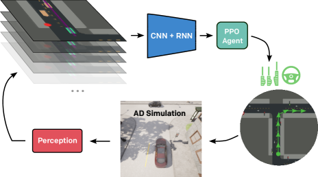
Figure 1: Our approach takes BEV images to learn driving policies in a simulated CARLA environment. Utilizing a CNN-based encoder while ensuring temporal understanding via an RNN, we learn longitudinal control using a PPO agent that predicts throttle and braking commands.

In this work, we discuss the challenges of constructing state representations for DRL of AD policies and present an efficient recurrent architecture as shown in Fig. 1 that exceeds previous methods based on a number of design choices. As demonstrated in previous approaches by Chen et al. [5, 6], DRL-based driving policies are highly dependent on low-dimensional state representations. Throughout this work, we investigate various semantic bird’s-eye-view (BEV) representations used for describing driving states. BEV representations may contain vehicles and pedestrians, planned high-level navigation routes, environment maps, and traffic light states. They serve as a highly capable representation while scaling to multiple agents [5] compared to classical approaches [3]. In addition, we argue that a significant number of perception tasks in AD are tackled in the BEV space, such as object detection [7], segmentation [8, 9], mapping [10] as well as tracking and forecasting [11]. Thus, addressing the AD task in BEV benefits from a considerable share of research in the aforementioned domains. In the following, we present an analysis of different BEV representations and propose RecurrDriveNet, an efficient recurrent learning architecture that captures the relevant features of the environment while reducing computational complexity. The novelty of RecurrDriveNet is that we use a long short-term memory (LSTM)-based encoding of a series of state transitions, which propagates the hidden state along full trajectories. We demonstrate its driving capability on a simulated AD task in CARLA [3], where it outperforms traditional learning paradigms that rely on frame-stacking.

Our main contributions can be summarized as follows:

• A novel recurrent architecture for efficient DRL in AD based on semantic BEV maps that minimizes collisions with other road users and respects traffic rules.

• Extensive experiments and ablations on variations of the BEV representation.

• We publish our code as part of this work: http://learning2drive.cs.uni-freiburg.de.

II Related Work

Learning control policies for AD either from demonstration or via reward design proves to be a challenging endeavor. This is not only due to the complexity of actions to take but also errors generated in the perception stage. Existing methods have taken different approaches to modeling state representations while producing low-dimensional intermediate representations. While it is possible to use raw sensor inputs obtained from real-world measurements [12], the vast majority of relevant works utilize CARLA for synthetic and pseudo-realistic data generation [3, 5, 13].

In general, we observe impressive performance in the area of representation learning from raw sensory inputs, namely RGB camera frontal view (FV) and LiDAR BEV to be used for decision-making [14, 15, 16, 17]. The majority of works approach the driving task in an end-to-end manner using RGB camera image FV and/or LiDAR BEV. Interestingly, the larger the perception backbone, the more we see approaches opting for IL [18, 15, 6, 19] instead of DRL. Thus, efficient state representations are still a considerable bottleneck when applying DRL to the problem at hand. Based on this, we classify related works based on the chosen state representations and modalities in the following.

The original CARLA paper introduced a robust, modular method with distinct modules for perception, planning, and control. It uses stacked $84\times 84$ FV images, a state vector including current speed, distance to the goal, and high-level navigation commands [3]. Some works regress driving-related affordances from temporal stacks of RGB FV images [20] that are fed to low-level controllers to infer commands, which effectively induces human bias in the system.

With the goal of incorporating multiple modalities, Chen et al. take a representation learning approach to generate pseudo-synthetic semantic BEV representations in an auto-encoding scheme from an RGB FV image as well as LiDAR data [17, 14, 5]. The produced BEV representations combine several map layers, namely drivable surface, planned route, stacked actor history, and stacked ego history, all at $64\times 64$ resolution. Even though these are prone to errors, they provide high interpretability, which is vital to the AD task. Interestingly, Chen et al. [16] take a knowledge distillation approach by first training a privileged teacher agent that has access to the ground truth (GT), which is in turn used to train a real-world student agent that takes only RGB FV images as input and is supervised by the teacher. Inspired by these advances, a number of approaches directly use GT information to synthetically generate BEV representations instead of obtaining these from raw sensor inputs. An IL approach by Chen et al. [6] uses BEV images of size $192\times 192$ that also include traffic light information along the planned route and stacked actor history. A DRL pendant to the aforementioned method [5] uses a smaller resolution of $64\times 64$ as high-dimensional state spaces still pose a considerable hurdle for DRL. Similarly, others [5, 13] opt for temporal stacking of BEV maps of resolution $128\times 128$ [13]. Notably, all these approaches do not make use of recurrent approaches in favor of frame-stacking.

Contrary to the BEV representation, Prakash et al. [15] learn multi-modal fusion with transformers from FV and LiDAR BEV. Similarly, Shao et al. [19] also include RGB surround view images to predict future waypoints auto-regressively. In contrast to this, DRL approaches usually predict driving control commands such as steering angle, throttle, and braking.

Most similar to our work, both Chen et al. [5] and Agarwal et al. [13] use semantic BEV state representations with access to GT information. While we benchmark different BEV representations for learning efficiency in the context of DRL, the focus of our work is the introduction of a recurrent learning scheme that propagates the hidden state along all steps of the observed trajectory. Alleviating the need for frame-stacking architectures ultimately leads to improved agent behavior given the chosen reward objective.

III Background

III-A Deep Reinforcement Learning for Autonomous Driving

The goal of DRL is to maximize a reward signal by learning the weights $\theta$ of an agent’s (stochastic) policy $\pi_{\theta}(a_{t}|s_{t})$ that maps actions $a_{t}$ to an observed state $s_{t}\in\mathcal{S}$. In AD, the state of the ego vehicle is typically defined by its own position, velocity, and planned trajectory as well as the state of other agents participating in the driving scenario. When action $a_{t}$ is applied, the agent observes a new state $s_{t+1}$ according to the state transitions probability $\mathcal{T}$. The function $\mathcal{R}$ defines the reward signal $r_{t}$; the discount factor $\gamma$ weights present to future rewards. Given an environment where an ego vehicle learns to interact with $N$ other road users, the system can then be described by a Markov decision process (MDP) with the tuple $(\mathcal{S},\mathcal{A},\mathcal{T},\mathcal{R},\gamma)$ modeling the other road users as part of the environment.

Since interaction-rich scenarios in AD involve $N\neq\operatorname{const}$ participating road users, a count-invariant state representation $s_{t}\in\mathcal{S}$ has to be found. This is due to the fact that the deep neural network (DNN) used in DRL require an input tensor of fixed size. Therefore, a common approach is to use a BEV-based state representation that encodes the state as an image. However, such image representations encode only spatial information. Due to the dynamic nature of interactions in AD, DRL agents must observe first and second-order derivatives of the vehicle dynamics too, i.e., velocity and acceleration. This information must either be encoded into ${s}_{t}$ directly or by opting for a temporal representation.

III-B Deep Reinforcement Learning Algorithm

Proximal policy optimization (PPO) [21] is an on-policy DRL algorithm using DNNs to learn a stochastic policy $\pi_{\theta_{k}}(a_{t}|s_{t})$. The DNN’s weights $\theta_{k}$ are updated by

$$\theta_{k+1}=\arg\max_{\theta}\underset{s_{t},a_{t}\sim\pi_{\theta_{k}}}{\mathrm{E}}\left[L\left(s_{t},a_{t},\theta_{k},\theta\right)\right],$$ (1)

at iteration $k+1$ for transition tuples $e_{t}=\{s_{t},a_{t},r_{t},s_{t+1}\}$ of a $T$ fixed-sized steps long trajectory $\tau=\{e_{0},e_{1},...,e_{T}\}$. The objective function $L\left(s_{t},a_{t},\theta_{k},\theta\right)$ is defined as

$$L\left(s_{t},a_{t},\theta_{k},\theta\right)=\min\biggl{(} \frac{\pi_{\theta}(a_{t}\mid s_{t})}{\pi_{\theta_{k}}(a_{t}\mid s_{t})}A^{\pi_{\theta_{k}}}(s_{t},a_{t}),$$

$$g\left(\epsilon,A^{\pi_{\theta_{k}}}(s_{t},a_{t})\right)\biggr{)}.$$ (2)

The advantage function $A=A^{\pi_{\theta_{k}}}(s_{t},a_{t})$ is used to calculate

$$g(\epsilon,A)=\begin{cases}(1+\epsilon)A&A\geq 0\\ (1-\epsilon)A&A<0\end{cases},$$ (3)

with the hyperparameter $\epsilon$. Due to $\epsilon$ and the min-clipping in (1), the policy updates are regularized to ensure smooth policy updates. To calculate the advantage function $A$ for (3), a common choice is the generalized advantage estimate (GAE) [22]. This method is based on a value function $V_{\phi_{k}}(s_{t})$ with weights $\phi_{k}$ that is learned based on

$$\phi_{k+1}=\arg\min_{\phi}\frac{1}{\left|\mathcal{D}_{k}\right|T}\sum_{\tau\in D_{k}}\sum_{t=0}^{T}\left(V_{\phi_{k}}\left(s_{t}\right)-\hat{R}_{t}\right)^{2},$$ (4)

with the reward-to-go $\hat{R}_{t}=\sum_{t^{\prime}=t}^{T}r_{t}$. The final regression target is obtained by estimating the expectation in (1) with $B$ recorded $T$-step long trajectories $\mathcal{D}_{k}=\{\tau_{0},\tau_{2},\dots,\tau_{B-1}\}_{k}$.

IV Methodology

In this work, we present a recurrent agent architecture for efficient DRL based on semantic bird’s-eye-view (BEV)maps, which serve as scalable state representations. We assume access to GT information in order to retrieve actor and environment data, which is in line with related works [13, 6]. The use of BEV representations is motivated by recent advancements [9, 10] and the fact that BEV images are sensor-agnostic representations. In the following, we describe spatial state representations (Sec. IV-A) as well as temporal state representations (Sec. IV-B) that allow making the agents’ dynamics observable as discussed in Sec. III-A.

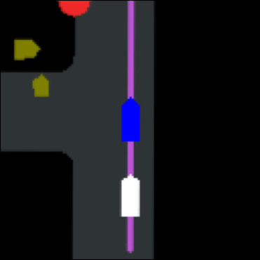
(a) RGB-BEV: Road geometry (gray), future waypoints (pink), traffic light states (green, yellow, red), ego vehicle (white), enlarged pedestrians (dark yellow), other vehicles (blue).

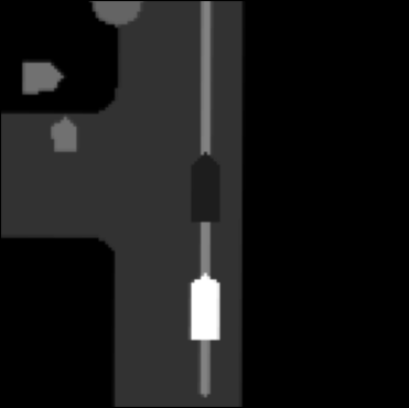
(b) Gray-BEV: Objects are encoded using distinct intensities in the gray spectrum that resemble the $\alpha$-channel of (a).

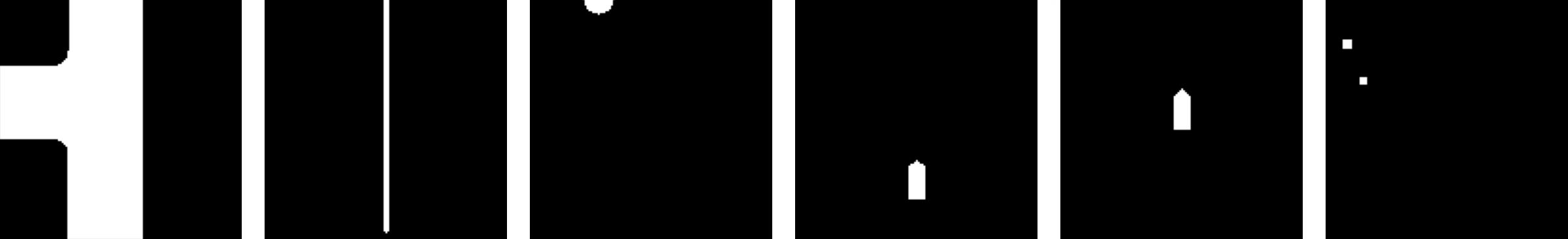
(c) Multi-BEV: The channels encode map geometry (# 1), future waypoints (# 2), traffic lights (# 3), ego vehicle (# 4), other vehicles (# 5), and pedestrians (# 6).

Figure 2: State representations as BEVs.

IV-A Spatial State Representations

We utilize a spatial state $s_{t}$ that encodes all actors as well as the immediate environment in a BEV image of the current driving scene. The pose of all road users is represented in an oriented bounding box fashion as shown in Fig. 2. Environment information is encoded by underlaying a map representation with lane information. As discussed in Sec. III-A, the chosen state representation is invariant to the number of participating road users. In the following, we discuss different variants of the BEV representation.

IV-A1 RGB Bird’s Eye View (RGB-BEV)

The BEV is represented by a quadratic image with 3 color channels (RGB) and dimension $3\times K\times K$. Different object types are color-coded in the image representation as shown in Fig. 2(a).

IV-A2 Grayscale Bird’s Eye View (Gray-BEV)

The RGB-BEV representation is converted to an image with a single channel in grayscale (Fig. 2(b)) but with the same properties, i.e., the representation has dimension $1\times K\times K$.

IV-A3 Multi-Channel Bird’s Eye View (Multi-BEV)

Instead of encoding the road user’s location into an RGB image, an image representation of dimension $6\times K\times K$ is used (Fig. 2(c)), with each of the six channels corresponding to a different property, respectively.

IV-B Temporal State Representations

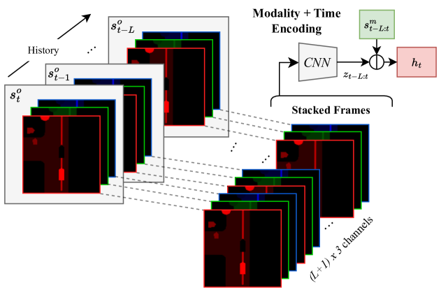
(a) Frame-stacking of sequences as used in [13, 5].

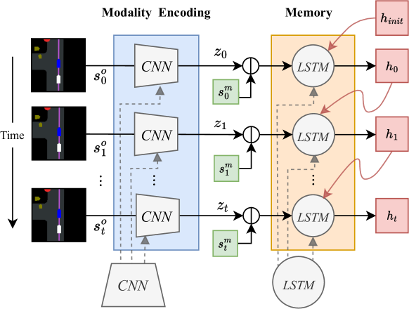
(b) LSTM-based encoding of trajectories (ours).

Figure 3: Sequential state representations and their encoding: Instead of stacking frames $s^{o}_{t}$ along $L+1$ frames as shown under (a), we encode BEV images using a recurrent architecture (b) in order to generate successive hidden states $h_{t}$ used for policy learning.

The BEV state representation in Sec. IV-A encodes the road users’ location into an image. However, the pure observation of such an image does not yield further insights into the road users states regarding linear velocity and acceleration. To make these properties observable, the frames can either be trivially stacked to form a history of previous observations or by employing recurrency along the trajectory of state transitions as we do (see Sec. IV-B2).

IV-B1 Frame-Stacking

The easiest way to include past information into the current state $s_{t}$ is to stack past observed states ${s_{t-1},s_{t-2},...,s_{t-L}}$ in terms of BEV images, i.e., the RGB-BEV representation becomes an $((L+1)\cdot 3)\times K\times K$ image, forming a history of the $L$ previous states as shown in Fig. 3(a). This history allows the DRL agents to observe the difference between subsequent states, which makes the other road users’ velocity and acceleration observable. This constitutes the method previous works followed [13, 5].

IV-B2 Recurrent Neural Network

Instead of encoding the history into the state representation itself, the use of recurrent neural networks (RNNs) allows the DRL agent to build a hidden state $h_{t}$ that is updated at every observed state $s_{t}$. The updated hidden state is accessed by the agent at the next time step again. This allows the agent to keep a memory of past observed states. In related works, RNNs are typically used to only encode the history of a sequence of frame-stacked images as described in Sec. IV-B1. Our presented architecture makes use of the full long-horizon capabilities of LSTMs by propagating the hidden state along the full trajectory of states as shown in Fig. 3(b).

IV-C RecurrDriveNet and Baselines

Based on the state representations outlined in Sec. IV-A and IV-B, we present the model of an AV that learns to drive in a simulated environment in CARLA [3]. This ego vehicle is implemented as a PPO agent consisting of a policy network $\pi_{\theta}$ and a value network $V_{\phi}$. In this context, we introduce our agent model called RecurrDriveNet, which combines the Multi-BEV state representation (Sec. IV-A) with an LSTM architecture. The novelty of RecurrDriveNet is that the hidden state $h_{t}$ is constantly propagated along each state of a trajectory (Fig. 3(b)) allowing for efficient long-horizon reasoning. This approach is only feasible because PPO is an on-policy algorithm that requires rollouts of trajectories. In Sec. V, we evaluate our proposed architecture across three different state representations. In the following, we point out the differences between these models.

IV-C1 Action Space

Based on available map data, the agent has to follow a planned trajectory of waypoints. These waypoints are generated randomly by a global planning module and the map’s lane graph. We employ a Stanley controller [23] for lateral control of the vehicle to simplify the action space of the agent so that only longitudinal control has to be learned. We justify this by arguing that the vehicle-pedestrian interaction in urban areas is mostly dependent on the longitudinal acceleration of the ego vehicle.

The ego vehicle’s action space is defined as $a_{t}\in[-1,1]$, which maps to the low-level control of a CARLA vehicle in the form of braking and throttle action, i.e., $-1$ means full brake, $0$ idle, and $+1$ corresponds to full throttle.

IV-C2 Observation Space

Instead of learning from raw sensor data such as RGB FV camera or LiDAR, we use GT perception for representing the ego-vehicle surroundings including other actors similar to others [13, 5]. Their position and orientation are then reflected in one of the BEV representations discussed in Sec. IV-A.

After encoding the state representation $s_{t}$ using a modality-encoder network (Fig. 3(b)), we concatenate the encodings $z_{t}$ with an ego-state vector $s_{t}^{m}$ that contains the following variables:

$$s_{t}^{m}=\Big{[}{\Delta}^{\text{traj}}_{t},{\delta}^{\text{traj}}_{t},{{v}}^{\text{ego}}_{t},{{\dot{v}}}^{\text{ego}}_{t},\alpha^{\text{ego}}_{t},{{v}}^{\text{lim}}_{t},{{f}}^{\text{red}}_{t}\Big{]}^{\top}.$$ (5)

The deviation from the planned trajectory is defined by the distance ${\Delta}^{\text{traj}}_{t}$ to the closest waypoint and the relative orientation ${\delta}^{\text{traj}}_{t}$ to it. The ego vehicle’s velocity, acceleration, and steering angle are ${{v}}^{\text{ego}}_{t}$, ${{\dot{v}}}^{\text{ego}}_{t}$, and $\alpha^{\text{ego}}_{t}$, respectively. The current allowed driving speed is given by ${{v}}^{\text{lim}}_{t}$. When the ego vehicle is close to a red traffic light, ${{f}}^{\text{red}}_{t}$ is set to $1.0$, $0.5$ when yellow, and otherwise to $0$.

IV-C3 Reward Function

Modified from [17], we define the reward function as:

$$r= v^{\text{ego}}_{\text{long}}-10\cdot f_{s}-0.2\cdot|\alpha|(v^{\text{ego}}_{\text{long}})^{2}-5\cdot\alpha^{2}$$

$$-f_{o}-200\cdot f_{v}-200\cdot f_{p}-200\cdot f_{r},$$ (6)

where each $f_{*}$ is set to 0 when the following corresponding conditions are not true. When the vehicle does not obey the permitted driving speed, $f_{s}$ evaluates to $f_{s}=1$. Excessive use of the steering angle $\alpha$ is penalized together with when the vehicle diverges more than 1$\mathrm{m}\text{/}$ from the planned trajectory by setting $f_{o}=1$. Additionally, collisions with pedestrians and other vehicles lead to a penalty with $f_{v}=1$ or $f_{p}=1$, respectively. When the ego vehicle runs a red traffic light, we set $f_{r}=1$.

IV-C4 Network Architecture

The agent’s policy network $\pi_{\theta}$ and the value network $V_{\phi}$ share a common modality-encoder to encode the BEV state $s^{o}_{t}$ to $z_{t}$. We deploy a convolutional neural network (CNN) with three convolutional layers $\{(32,8,4),(64,4,2),(64,3,2)\}$ with (#-filters, size, stride) and ReLU activation including a subsequent linear projection layer to $z_{t}\in\mathbb{R}^{256}_{+}$. The encodings $z_{t}$ are concatenated with the measurement vector $s^{m}_{t}$. For the LSTM-based agents, these combined encodings are fed to a single LSTM-layer with a hidden state of $h_{t}\in\mathbb{R}^{256}$. The LSTM’s output is then used in two separate modules of single linear layers for the policy and value network, respectively. Since the learned policy in PPO is stochastic, the agent learns the parameters of a $\operatorname{tanh}$-Normal distribution, i.e., a Gaussian distribution that is projected using a $\operatorname{tanh}$-function to the interval of $[-1,1]$. When no LSTM is used, the combined encoding is directly fed to the two modules with two instead of one linear layer.

V Experimental Evaluation

V-A Simulation Setup

Our proposed agent models are evaluated using the CARLA AD simulator  [3] that allows for imitating realistic traffic negotiation among both pedestrians and vehicles. We use the Town02 map, which resembles an urban area with single-lane roads and traffic lights but no roundabouts. Our simulation includes 30 other vehicles and 50 simulated pedestrians across the map that are controlled by CARLA. A LiDAR sensor with a range of $30\,$\mathrm{m}\text{/}$$, $110\,^{\circ}$ field of view, and no noise is used; traffic participants can be occluded. The action frequency is at $10\,$\mathrm{Hz}\text{/}$$.

V-B Implementation and Training Details

We train a total of six architectures for DRL in AD, as detailed in Table I and Table II. Our proposed RecurrDriveNet is based on the Multi-BEV state $s_{t}^{\text{Multi}}$ combined with an LSTM for recurrent connection. For all agents, the BEV image is a square image with $K=128$ pixels. The modality encoder’s first convolutional layer with $\text{stride}=4$ allows the use of high-resolution input images without increasing the output dimension significantly. Lower-resolution images suffer from ambiguity of the bounding box orientation, especially for pedestrians. The frame-stacking variants take the current and the previous $L=4$ observed frames as input.

All models are optimized for $1\,e\textsuperscript{6}$ steps with the same set of hyperparameters; reward and observations are normalized by a running mean calculation. We select $\gamma=0.999$, a clipping value of $\epsilon=0.1$ for PPO, and collect trajectories with a length of $128$ steps with four CARLA environments running in parallel. Further implementation details are accessible in our published code repository.

TABLE I: Combinations of state representations evaluated in this work. RecurrDriveNet is based on the state representation ${{s}_{t}^{\text{Multi}}+h_{t-1}}$.

	LSTM		Frame Stacking
	State $s_{t}$	dim	State $s_{t}$	dim
RGB-BEV	${s}_{t}^{\text{RGB}}+h_{t-1}$	$3\times 128^{2}$	${s}_{t-L:t}^{\text{RGB}}$	$15\times 128^{2}$
Gray-BEV	${s}_{t}^{\text{Gray}}+h_{t-1}$	$1\times 128^{2}$	${s}_{t-L:t}^{\text{Gray}}$	$5\times 128^{2}$
Multi-BEV	${s}_{t}^{\text{Multi}}+h_{t-1}$	$6\times 128^{2}$	${s}_{t-L:t}^{\text{Multi}}$	$30\times 128^{2}$

V-C Evaluation Metrics

The performance of the presented models is evaluated based on the occurrence of infractions while driving:

1. $I_{\text{veh}}$: # of vehicle collisions per distance in $\mathrm{1}\mathrm{/}\mathrm{k}\mathrm{m}$.

2. $I_{\text{ped}}$: # of pedestrians collisions over distance in $\mathrm{1}\mathrm{/}\mathrm{k}\mathrm{m}$.

3. $I_{\text{red}}$: # of run red traffic lights over distance in $\mathrm{1}\mathrm{/}\mathrm{k}\mathrm{m}$.

We further combine these in a metric termed $I_{\Sigma}$, which represents the sum across all infraction scores. The average violation with respect to the speed limit $v_{\text{lim}}^{\text{dev}}$ is given in $\%$. Additionally, we calculate the velocity $v^{\text{ego}}_{\text{move}}$ in $\mathrm{m}\text{/}\mathrm{s}$ when the ego-vehicle is moving faster than $0.2\,$\mathrm{m}\text{/}\mathrm{s}$$.

The results are evaluated on 320k simulation steps corresponding to a real-world driving time of almost 9 h.

V-D Training Results and Qualitative Assessment

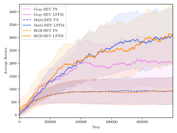
Figure 4: Comparison of the average returns produced by all model variants over the training time. We average across 3 runs per variant and display the associated standard deviation.

As shown in Figure 4, only the LSTM-based agents converge to a high average episodic return above 3000. We hypothesize that the models that use frame-stacking are stuck in local minima; they lack the long-horizon reasoning capability of the LSTM models. The Gray-BEV LSTM variant is superior to the frame-stacking approaches but does not achieve the high performance of the Multi-BEV LSTM (RecurrDriveNet) and RGB-BEV LSTM models. Despite similar training performance, further qualitative analysis shows that RecurrDriveNet’s Multi-BEV LSTM model outperforms the RGB-BEV LSTM variant by preventing infractions more reliably. We observe that all agents stop at large distances from other vehicles. While this behavior may be effective in preventing collisions, it leads to non-optimal traffic flow.

TABLE II: Quantitative results of our LSTM-based RecurrDriveNet for different state representations (Sec. IV) and comparison against traditional frame-stacking representations used by Chen et al. [5] and Agarwal et al. [13]. The displayed results represent each variant’s best results across 3 training runs.

Model	State Repr.	LSTM	FS	$I_{\Sigma}\downarrow$ [$\frac{}{\mathrm{km}}$]	$I_{\text{veh}}\downarrow$ [$\frac{}{\mathrm{km}}$]	$I_{\text{ped}}\downarrow$ [$\frac{}{\mathrm{km}}$]	$I_{\text{red}}\downarrow$ [$\frac{}{\mathrm{km}}$]	$v_{\text{lim}}^{\text{dev}}\downarrow$ [$\%$]	$v^{\text{ego}}_{\text{move}}$ [$\frac{\mathrm{m}}{\mathrm{s}}$]
	Gray-BEV		✓	$8.68$	$3.35$	$\boldsymbol{0.44}$	$4.89$	$2.93$	$7.00$
	RGB-BEV		✓	$8.30$	$2.86$	$0.46$	$4.98$	$3.02$	$6.95$
	Multi-BEV		✓	$8.47$	$2.92$	$0.51$	$5.03$	$1.26$	$6.82$
	Gray-BEV	✓		$3.65$	$2.90$	$0.67$	$0.08$	$2.78$	$5.85$
	RGB-BEV	✓		$1.24$	$0.25$	$0.93$	$\boldsymbol{0.06}$	$0.76$	$4.66$
RecurrDriveNet (ours)	Multi-BEV	✓		$\boldsymbol{0.75}$	$\boldsymbol{0.15}$	$0.54$	$0.07$	$1.41$	$4.67$

V-E Infraction Analysis

Table II presents the results of RecurrDriveNet compared to classical frame-stacking representations as used in previous works [13, 5]. First, we observe that only the LSTM-based architectures are able to learn a driving policy that is able to stop at red traffic lights. Second, RecurrDriveNet estimates the dynamic behavior of other road users successfully in order to prevent infractions as it achieves the lowest overall infraction score $I_{\Sigma}$ with a value of $0.75$ per driven kilometer. While all LSTM-based agents excel at obeying red traffic lights, i.e., infraction values $I_{\text{red}}$ of $0.06$, $0.07$, and $0.08$ for the RGB-BEV, Multi-BEV, and Gray-BEV state representations, respectively, only the Multi-BEV-based RecurrDriveNet has learned to reduce vehicle collisions to a minimum of $I_{\text{veh}}=0.15$. We reason that the Multi-BEV state has the advantage that each channel’s property is clearly separated from the remaining ones, i.e., a vehicle does not have to be detected across multiple channels. Similarly, the Gray-BEV is of much lower dimension compared to RGB-BEV. Interestingly, the pedestrian infractions of our RecurrDriveNet remain at a similar level as the other models with $I_{\text{veh}}=0.54$. This indicates that the BEV image representation struggles with representing pedestrian dynamics, e.g., probably due to smaller bounding boxes in the image and abrupt changes in the walking direction. The low performance of the frame-stacking representations corresponds to findings in previous work where frame-stacking approaches tend to work but require long training time, e.g., Agarwal et al. [13] trained their network for a total of $12\,e\textsuperscript{6}$ time steps compared to our $1e\,\textsuperscript{6}$ steps. Although RecurrDriveNet exhibits safe driving behavior, its driving is not overly cautious as a high moving velocity $v^{\text{ego}}_{\text{move}}=4.67\,$\frac{\mathrm{m}}{\mathrm{s}}$$ shows. Eventually, all agents comply with the set speed limits given by $v_{\text{lim}}^{\text{dev}}$.

VI Conclusion

While providing an extensive efficiency comparison of BEV representations used for AD, we presented a novel recurrent approach to learning urban driving policies from BEVs. The introduced RecurrDriveNet agent reduces collisions with other vehicles to a minimum while obeying traffic rules. Crucial to this approach is a LSTM-based learning paradigm for solving long-horizon driving. Our experiments show that this method surpasses frame-stacking-based methods used in the past. Follow-up work could address the incorporation of trajectory prediction methods in the BEV representation. The potential effects of the reward design on more efficient traffic flow should also be examined.

References

- [1] A. Millard-Ball, “Pedestrians, autonomous vehicles, and cities,” Journal of Planning Education and Research, vol. 38, pp. 6–12, 2018.
- [2] R. Trumpp, H. Bayerlein, and D. Gesbert, “Modeling interactions of autonomous vehicles and pedestrians with deep multi-agent reinforcement learning for collision avoidance,” in IEEE Intelligent Vehicles Symposium, 2022, pp. 331–336.
- [3] A. Dosovitskiy, G. Ros, F. Codevilla, A. Lopez, and V. Koltun, “CARLA: An open urban driving simulator,” in Conf. on Robot Learning, 2017, pp. 1–16.
- [4] F. Codevilla, E. Santana, A. M. López, and A. Gaidon, “Exploring the limitations of behavior cloning for autonomous driving,” in Int. Conf. on Computer Vision, 2019, pp. 9329–9338.
- [5] J. Chen, B. Yuan, and M. Tomizuka, “Model-free deep reinforcement learning for urban autonomous driving,” in Int. Conf. on Intelligent Transportation Systems, 2019, pp. 2765–2771.
- [6] ——, “Deep imitation learning for autonomous driving in generic urban scenarios with enhanced safety,” in Int. Conf. on Intelligent Robots and Systems, 2019, pp. 2884–2890.
- [7] J. Huang, G. Huang, Z. Zhu, Y. Yun, and D. Du, “Bevdet: High-performance multi-camera 3d object detection in bird-eye-view,” arXiv preprint arXiv:2112.11790, 2021.
- [8] N. Gosala and A. Valada, “Bird’s-eye-view panoptic segmentation using monocular frontal view images,” IEEE Robotics and Automation Letters, vol. 7, no. 2, pp. 1968–1975, 2022.
- [9] N. Gosala, K. Petek, P. L. Drews-Jr, W. Burgard, and A. Valada, “Skyeye: Self-supervised bird’s-eye-view semantic mapping using monocular frontal view images,” in Proc. of the IEEE Conf. on Computer Vision and Pattern Recognition, 2023, pp. 14 901–14 910.
- [10] M. Büchner, J. Zürn, I.-G. Todoran, A. Valada, and W. Burgard, “Learning and aggregating lane graphs for urban automated driving,” in Proc. of the IEEE Conf. on Computer Vision and Pattern Recognition, 2023, pp. 13 415–13 424.
- [11] A. Hu, Z. Murez, N. Mohan, S. Dudas, J. Hawke, V. Badrinarayanan, R. Cipolla, and A. Kendall, “Fiery: future instance prediction in bird’s-eye view from surround monocular cameras,” in Int. Conf. on Computer Vision, 2021, pp. 15 273–15 282.
- [12] A. Kendall, J. Hawke, D. Janz, P. Mazur, D. Reda, J.-M. Allen, V.-D. Lam, A. Bewley, and A. Shah, “Learning to drive in a day,” in Int. Conf. on Robotics and Automation, 2019, pp. 8248–8254.
- [13] T. Agarwal, H. Arora, and J. Schneider, “Learning urban driving policies using deep reinforcement learning,” in Int. Conf. on Intelligent Transportation Systems, 2021, pp. 607–614.
- [14] J. Chen, Z. Xu, and M. Tomizuka, “End-to-end autonomous driving perception with sequential latent representation learning,” in Int. Conf. on Intelligent Robots and Systems, 2020, pp. 1999–2006.
- [15] A. Prakash, K. Chitta, and A. Geiger, “Multi-modal fusion transformer for end-to-end autonomous driving,” in Proc. of the IEEE Conf. on Computer Vision and Pattern Recognition, 2021, pp. 7077–7087.
- [16] D. Chen, B. Zhou, V. Koltun, and P. Krähenbühl, “Learning by cheating,” in Conf. on Robot Learning, 2020, pp. 66–75.
- [17] J. Chen, S. E. Li, and M. Tomizuka, “Interpretable end-to-end urban autonomous driving with latent deep reinforcement learning,” IEEE Transactions on Intelligent Transportation Systems, vol. 23, no. 6, pp. 5068–5078, 2021.
- [18] D. Chen and P. Krähenbühl, “Learning from all vehicles,” in Proc. of the IEEE Conf. on Computer Vision and Pattern Recognition, 2022, pp. 17 222–17 231.
- [19] H. Shao, L. Wang, R. Chen, H. Li, and Y. Liu, “Safety-enhanced autonomous driving using interpretable sensor fusion transformer,” in Conf. on Robot Learning, 2023, pp. 726–737.
- [20] D. Coelho and M. Oliveira, “A review of end-to-end autonomous driving in urban environments,” IEEE Access, vol. 10, pp. 75 296–75 311, 2022.
- [21] J. Schulman, F. Wolski, P. Dhariwal, A. Radford, and O. Klimov, “Proximal policy optimization algorithms,” arXiv preprint arXiv:1707.06347, 2017.
- [22] J. Schulman, P. Moritz, S. Levine, M. Jordan, and P. Abbeel, “High-dimensional continuous control using generalized advantage estimation,” in Int. Conf. on Learning Representations, 2016.
- [23] G. M. Hoffmann, C. J. Tomlin, M. Montemerlo, and S. Thrun, “Autonomous automobile trajectory tracking for off-road driving: Controller design, experimental validation and racing,” in American control conference, 2007, pp. 2296–2301.