Improving Expressivity of GNNs with Subgraph-specific Factor Embedded Normalization

Abstract.

Graph Neural Networks (GNNs) have emerged as a powerful category of learning architecture for handling graph-structured data. However, existing GNNs typically ignore crucial structural characteristics in node-induced subgraphs, which thus limits their expressiveness for various downstream tasks. In this paper, we strive to strengthen the representative capabilities of GNNs by devising a dedicated plug-and-play normalization scheme, termed as SUbgraph-sPEcific FactoR Embedded Normalization (SuperNorm), that explicitly considers the intra-connection information within each node-induced subgraph. To this end, we embed the subgraph-specific factor at the beginning and the end of the standard BatchNorm, as well as incorporate graph instance-specific statistics for improved distinguishable capabilities. In the meantime, we provide theoretical analysis to support that, with the elaborated SuperNorm, an arbitrary GNN is at least as powerful as the 1-WL test in distinguishing non-isomorphism graphs. Furthermore, the proposed SuperNorm scheme is also demonstrated to alleviate the over-smoothing phenomenon. Experimental results related to predictions of graph, node, and link properties on the eight popular datasets demonstrate the effectiveness of the proposed method. The code is available at https://github.com/chenchkx/SuperNorm.

1. Introduction

Deep neural networks (DNNs) constitute a class of machine learning algorithms to learn representations of various data (He et al., 2016; Ye et al., 2023; Wang et al., 2023; Xu et al., 2023b; Chen et al., 2023; Ma et al., 2023; Xu et al., 2023a; Liu et al., 2022; Yang et al., 2022a, c; Yu et al., 2023; Li et al., 2023). In particular, Graph Neural Networks (GNNs) have emerged as the mainstream deep learning architectures to analyze irregular samples where information is present in the form of graph structure (Kipf and Welling, 2017; Veličković et al., 2018; Xu et al., 2019; Jing et al., 2021a; Dwivedi et al., 2022b; Jing et al., 2023b, a). As a powerful class of graph-relevant networks, these architectures have shown encouraging performance in various domains such as cell clustering (Li et al., 2022; Alghamdi et al., 2021), chemical prediction (Tavakoli et al., 2022; Zhong et al., 2022), social networks (Bouritsas et al., 2022; Dwivedi et al., 2022b), image style transfer (Jing et al., 2022, 2021b), traffic networks (Bui et al., 2021; Li and Zhu, 2021), combinatorial optimization (Schuetz et al., 2022; Cappart et al., 2021; Wang et al., 2021), and power grids (Yang et al., 2022b; Boyaci et al., 2021; Chen et al., 2022a). These successful applications can be actually classified into various downstream tasks, e.g., node, link (Gupta et al., 2021; Chen et al., 2022d), and graph predictions (Chen et al., 2022b; Han et al., 2022).

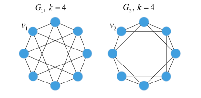
(a) Two $k$-regular graph

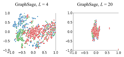
(b) Over-smoothing phenomenon

Figure 1. (a) The illustration of two different $k$-regular graphs, where $k=4$ in $G_{1}$ and $G_{2}$. (b) The t-SNE illustration of over-smoothing issue on Cora dataset (show the first three categories).

Most existing GNNs employ the message-passing scheme to learn node features from local neighborhoods, ignoring the unique characteristics of node-induced subgraphs, consequently limiting the expressive capability of GNNs. Specifically, the expressive capability of such GNNs is at most as powerful as that of the Weisfeiler-Leman (1-WL) (Weisfeiler and Leman, 1968) test to distinguish non-isomorphism graphs (Xu et al., 2019). An example is shown in Figure 1(a), where it is still challenging for existing GNNs to separate the two $k$-regular graphs $G_{1}$ and $G_{2}$. Furthermore, the advances in recent researches (Li et al., 2018; Zhao and Akoglu, 2020) show that the formulation of GNNs is a particular format of Laplacian smoothing, which thereby results in the over-smoothing issue, especially when GNNs go deeper, as shown in Figure 1(b). As a result of increasing layer numbers, GNNs are typically prone to indistinguishable representations for node and link predictions (Gupta et al., 2021; Chen et al., 2022d).

In this paper, we develop a new normalization framework which is SuperNorm, compensating for the ignored characteristics among the node-induced subgraph structures, to improve the graph expressivity over the prevalent message-passing GNNs for various graph downstream tasks. Our proposed normalization, with subgraph-specific factor embedding, enhances the GNNs’ expressivity to be at least as powerful as 1-WL test in distinguishing non-isomorphic graphs. Moreover, SuperNorm can help alleviate the oversmoothing issue in deeper GNNs. The contributions of this work can be summarized as follows:

• We propose a method to compute subgraph-specific factors by performing a hash function on the number of nodes and edges, as well as the eigenvalues of the adjacency matrix, which is proved to be exclusive for each non-isomorphic subgraph.

• We develop a novel normalization scheme (i.e., SuperNorm), with subgraph-specific factor embedding, to strengthen the expressivity of GNNs, which can be easily generalized in arbitrary GNN architectures for various downstream tasks.

• We provide both the experimental and the theoretical analysis to support the claim that SuperNorm can extend GNNs to be at least as powerful as the 1-WL test in distinguishing non-isomorphism graphs. In addition, we also prove that SuperNorm can help alleviate over-smoothing issue.

2. Preliminary

In this section, we begin by introducing the notation for GNNs, along the way, understanding the issue of the graph isomorphism test and the over-smoothing phenomenon in GNNs.
Notation. Let $G=(V_{G},E_{G})$ denotes a undirected graph with $n$ vertices and $m$ edges, where $V_{G}$$=\{v_{1},v_{2},..v_{n}\}$ is an unordered set of vertices and $E_{G}\subseteq V_{G}\times V_{G}$ is a set of edges. $\mathcal{N}(v)=\{u\in V_{G}|(v,u)\in E_{G}\}$ denotes the neighbor set of vertex $v$, and its neighborhood subgraph $S_{v}$ is induced by $\tilde{\mathcal{N}}(v)=\mathcal{N}(v)\cup{v}$, which contains all edges in $E_{G}$ that have both endpoints in $\tilde{\mathcal{N}}(v)$. As shown in Figure 2, $S_{v_{1}}$ and $S_{v_{2}}$ are the induced subgraphs of $v_{1}$ and $v_{2}$ in Figure 1(a). The feature matrix $\text{H}=[h_{1},h_{2},...,h_{n}]\in\mathds{R}^{n\times d}$ is the learned feature from GNNs, where $d$ is the embedded dimension.

2.1. Graph Isomorphism Issue

The graph isomorphism issue is a challenging problem of determining whether two finite graphs are topologically identical. The WL algorithm (Weisfeiler and Leman, 1968), i.e., 1-WL for notation simplicity, is a well-established framework and computationally-efficient that distinguishes a broad class of graphs. In details, 1-WL refines color by iteratively aggregating the labels of nodes and hashing the aggregated multiset into unique labels, and its formulation can be represented as:

(1) $$\begin{split}h_{v}^{(t)}=\texttt{Hash}(h_{v}^{t-1},\mathcal{A}\{h_{u}^{t-1}|u\in\mathcal{N}(v)\}),\\ \end{split}$$

where $h_{v}^{(t)}$ is the $t$-th layer representation of node $v$. $\mathcal{A}$ is the aggregating function to aggregate its neighbors’ labels, and Hash is the injective mapping function to get a unique new label. However, 1-WL can not distinguish subtree-isomorphic subgraphs, e.g., $S_{v_{1}},S_{v_{2}}$ in Figure 2, which are defined as follow:

Definition 0.

Following the definition in (Wijesinghe and Wang, 2022), $S_{v_{i}}$ and $S_{v_{j}}$ are subtree-isomorphic, $S_{v_{i}}{\simeq}_{\texttt{subtree}}S_{v_{j}}$, if there exists a bijective mapping $f:$ $\tilde{\mathcal{N}}$$(v_{i})\rightarrow$ $\tilde{\mathcal{N}}$$(v_{j})$ such that $f(v_{i})=v_{j}$ and for any $v^{\prime}\in$ $\tilde{\mathcal{N}}$$(v_{i})$ and $f(v^{\prime})=u^{\prime},h_{v^{\prime}}=h_{u^{\prime}}$.

Expressivities of GNNs. GNNs’ expressivities are as powerful as the 1-WL test in distinguishing non-isomorphic graphs while any two different subgraphs $S_{v_{i}}$, $S_{v_{j}}$ are subtree-isomorphic (i.e., $S_{v_{i}}\simeq_{\texttt{subtree}}S_{v_{j}}$), or GNNs can map two different subgraphs into two different embeddings if and only if $S_{v_{i}}\not\simeq_{\texttt{subtree}}S_{v_{j}}$.

Theorem 2.

GNNs are as powerful the as 1-WL test in distinguishing non-isomorphic graphs while any two different subgraphs $S_{v_{i}}$, $S_{v_{j}}$ are subtree-isomorphic (i.e., $S_{v_{i}}\simeq_{\texttt{subtree}}S_{v_{j}}$), or GNNs can map two different subgraphs into two different embeddings if and only if $S_{v_{i}}\not\simeq_{\texttt{subtree}}S_{v_{j}}$.

Proof.

The complete proof is provided in Appendix A.1. ∎

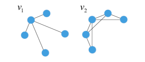
Figure 2. The illustration of subtree-isomorphic, i.e., two induced subgraphs of $v_{1}$ and $v_{2}$ from $G_{1}$ and $G_{2}$ in Figure 1(a).

2.2. Over-smoothing Issue

Although the message-passing mechanism helps us to harness the information encapsulated in the graph structure, it may introduce some limitations when combined with GNN’s depth. For the convolution operation of GNNs, a graph structure $G$ can be equivalently defined as an adjacency matrix $\text{A}\in\mathds{R}^{n\times n}$ to update node features with the degree matrix ${\text{D}}=\text{diag}(\text{deg}_{1},\text{deg}_{2},...,\text{deg}_{n})\in\mathds{R}^{n\times n}$. Let $\tilde{\text{A}}=\text{A}+\text{I}$ and $\tilde{\text{D}}=\text{D}+\text{I}$ denote the augmented adjacency and degree matrices by adding self-loops. $\tilde{\text{A}}_{\texttt{sym}}=\tilde{\text{D}}^{-1/2}\tilde{\text{A}}\tilde{\text{D}}^{-1/2}$ and $\tilde{\text{A}}_{\texttt{rw}}=\tilde{\text{D}}^{-1}\tilde{\text{A}}$ represent symmetrically and nonsymmetrically normalized adjacency matrices, respectively. Given the input node feature matrix $\text{H}^{t-1}$, the basic formulation of GNNs convolution follows:

(2) $$\begin{split}\text{H}^{t}=(\text{I}-\alpha\text{I})\text{H}^{t-1}+\alpha\tilde{\text{\text{A}}}_{\texttt{rw}}\text{H}^{t-1},\end{split}$$

where graph convolution usually lets $\alpha=1$ and uses the symmetrically normalized Laplacian to obtain $\text{H}^{t}=\tilde{\text{A}}_{\texttt{sym}}\text{H}^{t-1}$. To analyze GNNs’ working mechanism, Li et al. (Li et al., 2018) showed that the graph convolution is a particular form of Laplacian smoothing, which makes the node representation from different clusters become mixed up. Furthermore, Zhao et al. (Zhao and Akoglu, 2020) discovered that Laplacian smoothing washes away the information from all the features, i.e. the representations with regard to different columns of the feature matrix, and thus makes nodes indistinguishable.
Representatives of GNNs. As a natural result of GNNs going deeper, node representations become similar, and signals are washed away. Therefore, sample representations from different clusters become indistinguishable so that GNNs’ performance suffers from this phenomenon for node-relevant tasks, e.g., node and link classification (Gupta et al., 2021; Chen et al., 2022d).

3. Subgraph-specific Factor Embedded Normalization

We first present the subgraph-specific factor that uniquely distinguish various non-isomorphism subgraphs. Then, we present a graph normalization framework, i.e., SuperNorm, which improves GNNs’ expressivity by embedding the subgraph-specific factor. Finally, we provide the theoretical analysis to support the claim that SuperNorm can generally extend GNNs expressivity for various tasks.

3.1. Subgraph-specific Factor

We propose the subgraph-specific factor, a computable quantity for distinguishing non-isomorphism subgraphs, by considering the following two cases:

• Subgraphs are not subtree-isomorphic, i.e., these subgraphs have different numbers of nodes, and can be distinguished by the node’s number. In this condition, the subgraph-specific factor is related to node’s number and is representes as $\varphi(|V_{S_{v_{i}}}|)$, where $|\cdot|$ denotes cardinality and $\varphi(\cdot)$ is an arbitrary injective function.

• Subgraphs are subtree-isomorphic, i.e., these subgraphs have the same numbers of nodes, but can be distinguished by the set of eigenvalues ${\rm Eig}=\{e_{0},e_{1},...,e_{n-1}\}$ of the adjacency matrix . In this condition, the subgraph-specific factor is the result of injective function over eigenvalues, i.e., $\psi({\rm Eig}_{S_{v_{i}}})$.

By comprehensively considering these two cases, we can uniquely determine a subgraph structure, and thus develop the final subgraph-specific factor $\xi(S_{v_{i}})$ by utilizing hash function:

(3) $$\begin{split}\xi(S_{v_{i}})=\texttt{Hash}(\varphi(|V_{S_{v_{i}}}|),\psi({\rm Eig}_{S_{v_{i}}})).\\ \end{split}$$

where the adopt Hash function in this paper is the polynomial rolling hash function (PloyHash) (Karp and Rabin, 1987), which is often designed as an injection function with a low probability of hash collisions (Gusfield, 1997; Leiserson et al., 1994), and is widely used in applications such as string matching and fingerprinting. Therefore, the PloyHash can be used as an injective mapping function over the multiset in practice, which is suitable to compute distinguishable factors for identifying subgraphs. The definition is as follows.

Definition 0.

Polynomial rolling hash function (PloyHash) is a hash function that uses only multiplications and additions. Given a multiset $S=\{s_{0},s_{1},...,s_{n-1}\}$, PloyHash is:

(4) $$\begin{split}{\rm\texttt{PloyHash}}(S)=s_{0}+s_{1}\cdot p+s_{2}\cdot p^{2},...,+s_{n-1}\cdot p^{n-1}\;,\end{split}$$

where $p$ is a constant and $n$ is the number of input elements.

Implementation. We also use PloyHash as the injective function $\psi({\rm Eig}_{S_{v_{i}}})$ on eigenvalues. Moreover, we additionally use a powerful weight (Wijesinghe and Wang, 2022), i.e., $\mathcal{D}(S_{v_{i}})=2|E_{S_{v_{i}}}|/(|V_{S_{v_{i}}}|\cdot(|V_{S_{v_{i}}}|-1))\cdot{|V_{S_{v_{i}}}|}^{2}$, to increase the capability of factors. Therefore, the Eq.(3) can be rewritten as $\xi(S_{v_{i}})=\texttt{PloyHash}(\mathcal{D}(S_{v_{i}}),\varphi(|V_{S_{v_{i}}}|),$ $\psi({\rm Eig}_{S_{v_{i}}}))$.

3.2. SuperNorm for GNNs

Standard normalization can be empirically divided into two stages, i.e., centering $\&$ scaling (CS) and affine transformation (AT) operations. For the input features $\text{H}\in\mathds{R}^{n\times d}$, the CS and AT follow:

(5) $$\begin{split}\texttt{CS}\;\text{:}\;&\text{H}_{\texttt{CS}}=\frac{\text{H}-\mathds{E}(\text{H})}{\sqrt{\mathds{D}\text{(H)}+\epsilon}},\\ \texttt{AT}\;\text{:}\;&\text{H}_{\texttt{AT}}=\text{H}_{\texttt{CS}}\odot\gamma+\beta,\\ \end{split}$$

where $\odot$ is the dot product with the broadcast mechanism. $\mathds{E}(\text{H})$ and $\mathds{D}(\text{H})$ denote mean and variance statistics, and $\gamma$, $\beta$ $\in\mathds{R}^{1\times d}$ are the learned scale and bias factors. The main drawback of the existent normalizations is the absence of subgraph information, which downgrades the expressivity to distinguish, e.g., isomorphic graphs and other graph symmetries. In this paper, we aim to embed factor $\xi(S_{v_{i}})$ into BatchNorm, and thus take a batch of graphs for example.

Batch Graphs. For a bacth of graphs $\mathcal{G}=\{G_{1},...,G_{m}\}$ with node set $V_{\mathcal{G}}=V_{G_{1}}$$\cup$ $V_{G_{2}}$$,...,V_{G_{m}}$ $=\{v_{1},v_{2},...,v_{n}\}$ and feature matrix $\text{H}\in\mathds{R}^{n\times d}$. Subgraph-specific factor of this batch nodes is represented as $\text{M}_{\mathcal{G}}$$=\xi(S_{V_{\mathcal{G}}})=[\xi(S_{V_{G_{1}}});\xi(S_{V_{G_{2}}})$$;...;\xi(S_{V_{G_{m}}})]=[\xi(S_{v_{1}}),\xi(S_{v_{2}}),$ …, $\xi(S_{v_{n}})]$$\in\mathds{R}^{n\times 1}$. The segment summation-normalization $\text{M}_{\texttt{SN}}$$=[\mathcal{F}(\xi(S_{V_{G_{1}}}));...;\mathcal{F}(\xi(S_{V_{G_{m}}}))$$]$$\in\mathds{R}^{n\times 1}$ where $\mathcal{F}$$(\xi(S_{V_{G_{i}}}))=\xi(S_{V_{G_{i}}})$ $/\sum\xi(S_{V_{G_{i}}})\in\mathds{R}^{|V_{G_{i}}|\times 1}$, denotes the summation-normalization operation in each graph.

To establish the SUbgraph-sPEcific factoR embedded normalization (SuperNorm), we develop two strategies, i.e., representation calibration (RC) and representation enhancement (RE) as follow:

3.2.1. Representation Calibration (RC)

Before the CS stage, we calibrate the inputs by injecting the subgraph-specific factor as well as incorporate the graph instance-specific statistics into representations, which balances the distribution differences along with embedding structural information. For the input feature $\text{H}\in\mathds{R}^{n\times d}$, the RC is formulated as:

(6) $$\begin{split}\texttt{RC}\;\text{:}\;\text{H}_{\texttt{RC}}=\text{H}+w_{\texttt{RC}}\odot\text{H}_{\texttt{SA}}\cdot(\text{M}_{\texttt{RC}}\mathds{1}_{d}^{T}),\end{split}$$

where $\cdot$ denotes the dot product operation and $\mathds{1}_{d}$ is the $d$-dimensional all-one cloumn vectors. $w_{\texttt{RC}}\in\mathds{R}^{1\times d}$ is a learned weight parameter. $\text{M}_{\texttt{RC}}=\text{M}_{\texttt{SN}}\cdot\text{M}_{\mathcal{G}}\in\mathds{R}^{n\times 1}$ is the calibration factor for RC, which is explained in details in Appendix A.2. $\text{H}_{\texttt{SA}}\in\mathds{R}^{n\times d}$ is the segment averaging of H, obtained by sharing the average node features of each graph with its nodes, where each individual graph is called a segment in the DGL implementation (Wang et al., 2019).

3.2.2. Representation Enhancement (RE)

Right after the CS operation, node features $\text{H}_{\texttt{CS}}$ are constrained into a fixed variance range and distinctive information is slightly weakened. Thus, we design the RE operation to embed subgraph-specific factor into AT stage for the enhancement the final representations. The formulation of RE is written as follows:

(7) $$\begin{split}\texttt{RE}\;\text{:}\;&\text{H}_{\texttt{RE}}=\text{H}_{\texttt{CS}}\cdot\texttt{Pow}{(\text{M}_{\texttt{RE}},{w_{\texttt{RE}})}},\\ \end{split}$$

where $w_{\texttt{RE}}\in\mathds{R}^{1\times d}$ is a learned weight parameter, and $\texttt{Pow}(\cdot)$ is the exponential function. To imitate affine weights in AT for each channel, we perform the segment summation-normlization on calibration factor $\text{M}_{\texttt{RC}}$ and repeats $d$ columns to obtain enhancement factor $\text{M}_{\texttt{RE}}$$\in\mathds{R}^{n\times d}$ , which ensures column signatures of $\texttt{Pow}{(\text{M}_{\texttt{RE}},{w_{\texttt{RE}})}}-1$ are consistent.

3.2.3. The Implementation of SuperNorm.

At the implementation stage, we merge RE operation into AT for a simpler formultation description. Given the input feature $\text{H}\in\mathds{R}^{n\times d}$, the formulation of the SuperNorm is written as:

(8) $$\begin{split}\texttt{RC}\;\text{:}\;&\text{H}_{\texttt{RC}}=\text{H}+w_{\texttt{RC}}\odot\text{H}_{\texttt{SA}}\cdot(\text{M}_{\texttt{RC}}\mathds{1}_{d}^{T}),\\ \texttt{CS}\;\text{:}\;&\text{H}_{\texttt{CS}}=\frac{\text{H}_{\texttt{RC}}-\mathds{E}(\text{H}_{\texttt{RC}})}{\sqrt{\mathds{D}(\text{H}_{\texttt{RC}})+\epsilon}},\\ \texttt{AT}\;\text{:}\;&\text{H}_{\texttt{AT}}=\text{H}_{\texttt{CS}}\cdot(\gamma+\mathds{P})/2+\beta,\\ \end{split}$$

where $\mathds{P}=\texttt{Pow}{(\text{M}_{\texttt{RE}},{w_{\texttt{RE}})}}$. $\text{H}_{\texttt{AT}}$ is the output of SuperNorm. To this end, we add RC and RE operations at the beginning and ending of the original BatchNorm layer to strengthen the expressivity power after GNNs’ convolution.
Please note that the subgraph-specific factors are preprocessed in the dataset, and the RC and RE operations are the dot product in $\mathds{R}^{n\times d}$. Therefore, the additional time complexity is $\mathcal{O}(nd)$.

3.3. Theoretical Analysis.

SuperNorm with subgraph-specific factor embedding, compensating structural characteristics of subgraphs, can generally improve GNNs’ expressivity as follows:

(1) Graph-level: For graph prediction tasks, SuperNorm compensates for the subgraph information to distinguish the subtree-isomorphic case that 1-WL can not recognize. Specifically, an arbitrary GNN equipped with SuperNorm is at least as powerful as the 1-WL test in distinguishing non-isomorphic graphs, The detalied analysis is provided in the Theorem 2.

(2) Node-level: The ignored subgraph information strengthens the node representations, which is beneficial to the downstream recognition tasks. Furthermore, SuperNorm with subgraph-specific factor injected can help alleviate the oversmoothing issue, which is analyzed in the following Theorem 3.

(3) Training stability: The RC operation is beneficial to stablilize model training, which makes normalization operation less reliant on the running means and balances the distribution differences among batches, and is analyzed in the following Proposition 4.

Theorem 2.

SuperNorm extends GNNs’ expressivity to be at least as powerful as 1-WL test in distinguishing non-isomorphic graphs.

Proof.

For the non-isomorphic graphs distinguishing issue, we follow the analysis procedure in the proof of Theorem 2, i.e., taking subtree-isomorphic substructures, for example.

• When $S_{v_{i}}\simeq_{\texttt{subtree}}S_{v_{j}}$, GNNs’ expressivity is as powerful as 1-WL test in distinguishing non-isomorphic graphs. However, GNNs with the subgraph-specific factor embedding can distinguish subtree-isomorphic substructure, where 1-WL misses the distinguishable power. In this case, GNNs are more expressive than 1-WL test.

• When $S_{v_{i}}\not\simeq_{\texttt{subtree}}S_{v_{j}}$ and $\mathcal{M}$ map two different substructures into different representations (i.e., $f(S_{v_{i}})\neq f(S_{v_{j}})$), which means that $\mathcal{M}$ distinguish these two substructures like Hash in 1-WL. In this case, SuperNorm further improve GNNs’ expressivity in distinguishing graphs.

• When $S_{v_{i}}\not\simeq_{\texttt{subtree}}S_{v_{j}}$ and $\mathcal{M}$ transforms two different substructures into the same representation,  GNNs are not as powerful as 1-WL test in distinguishing non-isomorphic graphs. However, SuperNorm can improve the graph expressivity of GNNs to be as powerful as 1-WL test.

According to the above three items, we can conclude that SuperNorm can extend GNNs’ expressivity to be at least as powerful as 1-WL test in distinguishing non-isomorphic graphs

The proof of Theorem 2 is complete. ∎

Theorem 3.

SuperNorm helps alleviate the oversmoothing issue.

Proof.

Given two extremely similar embeddings of $u$ and $v$ (i.e., $\lVert\text{H}_{u}-\text{H}_{v}\rVert_{2}\leq\epsilon$). Assume for simplicity that $\lVert\text{H}_{u}\rVert_{2}=\lVert\text{H}_{v}\rVert_{2}=1$, $\|w_{\texttt{RC}}\|_{2}\geq c_{1}$, and the subgraph-specific factors between $u$ and $v$ differs a considerable margin $\|(\text{M}_{\texttt{RC}}\mathds{1}_{d}^{T})_{u}-(\text{M}_{\texttt{RC}}\mathds{1}_{d}^{T})_{v}\|_{2}\geq 2\epsilon/c_{1}$. Following the RC operation in Eq.(6), we can obtain the following formula derivation:

$$\begin{split}&\lVert(\text{H}_{u}+{(w_{\texttt{RC}}\odot(\text{M}_{\texttt{RC}}\mathds{1}_{d}^{T}))}_{u}\cdot\frac{\text{H}_{u}+\text{H}_{v}}{2})\\ &\qquad-(\text{H}_{v}+{(w_{\texttt{RC}}\odot(\text{M}_{\texttt{RC}}\mathds{1}_{d}^{T}))}_{v}\cdot\frac{\text{H}_{v}+\text{H}_{u}}{2})\rVert_{2}\\ &\geq-\|\text{H}_{u}-\text{H}_{v}\|_{2}+\|({(w_{\texttt{RC}}\odot(\text{M}_{\texttt{RC}}\mathds{1}_{d}^{T}))}_{u}\\ &\qquad-{(w_{\texttt{RC}}\odot(\text{M}_{\texttt{RC}}\mathds{1}_{d}^{T}))}_{v})\cdot\frac{\text{H}_{u}+\text{H}_{v}}{2}\|_{2}\\ &\geq-\epsilon+\|w_{\texttt{RC}}\|_{2}\cdot\|(\text{M}_{\texttt{RC}}\mathds{1}_{d}^{T})_{u}-(\text{M}_{\texttt{RC}}\mathds{1}_{d}^{T})_{v}\|_{2}\cdot\|\frac{\text{H}_{u}+\text{H}_{v}}{2}\|_{2}\\ &\geq-\epsilon+2\epsilon=\epsilon,\end{split}$$

where the subscripts $u$, $v$ denote the $u$-th and $v$-th row of matrix $\in\mathds{R}^{n\times d}$. This inequality demonstrates that our RC operation could differentiate two nodes by a margin $\epsilon$ even when their node embeddings become extremely similar after $L$-layer GNNs. Similarly, by assuming $\|\texttt{Pow}{(\text{M}_{\texttt{RE}},{w_{\texttt{RE}})}}_{u}\|_{2}\leq c_{2}$ and $\|\texttt{Pow}{(\text{M}_{\texttt{RE}},{w_{\texttt{RE}})}}_{u}-\texttt{Pow}{(\text{M}_{\texttt{RE}},{w_{\texttt{RE}})}}_{v}\|_{2}\geq(1+c_{2})\cdot\epsilon$, we can prove that the RE operation differentiates the embedding with subgraph-specific factor:

$$\begin{split}&\lVert\texttt{Pow}{(\text{M}_{\texttt{RE}},{w_{\texttt{RE}})}}_{u}\cdot\text{H}_{u}-\texttt{Pow}{(\text{M}_{\texttt{RE}},{w_{\texttt{RE}})}}_{v}\cdot\text{H}_{v}\rVert_{2}\\ &=\lVert\texttt{Pow}{(\text{M}_{\texttt{RE}},{w_{\texttt{RE}})}}_{u}\cdot(\text{H}_{u}-\text{H}_{v})+(\texttt{Pow}{(\text{M}_{\texttt{RE}},{w_{\texttt{RE}})}}_{u}\\ &\quad-\texttt{Pow}{(\text{M}_{\texttt{RE}},{w_{\texttt{RE}})}}_{v})\cdot\text{H}_{v}\rVert_{2}\\ &\geq-\lVert\texttt{Pow}{(\text{M}_{\texttt{RE}},{w_{\texttt{RE}})}}_{u}\cdot(\text{H}_{u}-\text{H}_{v})\rVert_{2}+\lVert(\texttt{Pow}{(\text{M}_{\texttt{RE}},{w_{\texttt{RE}})}}_{u}\\ &\quad-\texttt{Pow}{(\text{M}_{\texttt{RE}},{w_{\texttt{RE}})}}_{v})\cdot\text{H}_{v}\rVert_{2}\\ &\geq-c_{2}\cdot\epsilon+(1+c_{2})\cdot\epsilon=\epsilon.\\ \end{split}$$

The proof is complete. ∎

Proposition 0.

RC operation is beneficial to stabilzing the model training.

Proof.

The RC operation is formulated as

(9) $$\begin{split}\texttt{RC}\;\text{:}\;&\text{H}_{\texttt{RC}}=\text{H}+w_{\texttt{RC}}\odot\text{H}_{\texttt{SA}}\cdot(\text{M}_{\texttt{RC}}\mathds{1}_{d}^{T}),\\ \end{split}$$

where and $\mathds{1}_{d}$ is $d$-dimensional all-one column vector. Here $\text{H}_{\texttt{SA}}$ introduces the current graph’s instance-specific information, i.e., mean representations in each graph. $w_{\texttt{RC}}$ is a learnable weight balancing mini-batch and instance-specific statistics. Assume the number of nodes in each graph is consistent. The expectation of input features after RC, i.e., $\mathds{E}(\text{H}_{\texttt{RC}})$, can be represented as

(10) $$\begin{split}\mathds{E}(\text{H}_{\texttt{RC}})=(1+w_{\texttt{RC}}\odot(\text{M}_{\texttt{RC}}\mathds{1}_{d}^{T}))\cdot\mathds{E}(\text{H}).\\ \end{split}$$

Let us respectively consider the following centering operation of normalization for the original input H and the feature matrix $\text{H}_{\texttt{RC}}$ after RC operation,

(11) $$\begin{split}\text{H}_{\texttt{Center-In}}&=\text{H}-\mathds{E}(\text{H}),\\ \text{H}_{\texttt{Center-RC}}&=\text{H}_{\texttt{RC}}-\mathds{E}(\text{H}_{\texttt{RC}}),\\ \end{split}$$

where $\text{H}_{\texttt{Center-In}}$ and $\text{H}_{\texttt{Center-RC}}$ denote the centering operation on H and $\text{H}_{\texttt{RC}}$. To compare the difference between these two centralized features, we perform

(12) $$\begin{split}&\text{H}_{\texttt{Center-RC}}-\text{H}_{\texttt{Center-In}}\\ &=(\text{H}_{\texttt{RC}}-\mathds{E}(\text{H}_{\texttt{RC}}))-(\text{H}-\mathds{E}(\text{H}))\\ &=\text{H}+w_{\texttt{RC}}\odot(\text{M}_{\texttt{RC}}\mathds{1}_{d}^{T})\cdot\text{H}_{\texttt{SA}}-(1+w_{\texttt{RC}}\odot(\text{M}_{\texttt{RC}}\mathds{1}_{d}^{T}))\cdot\mathds{E}(\text{H})\\ &\quad-(\text{H}-\mathds{E}(\text{H}))\\ &=w_{\texttt{RC}}\odot(\text{M}_{\texttt{RC}}\mathds{1}_{d}^{T})\cdot(\text{H}_{\texttt{SA}}-\mathds{E}(\text{H})),\\ \end{split}$$

where the values in $\text{M}_{\texttt{RC}}$ are always positive numbers. When values in $w_{\texttt{RC}}$ are close to zero, the centering operation still relies on running statistics over the training set. On the other hand, the importance of graph instance-specific statistics grows when the absolute value of $w_{\texttt{RC}}$ becomes larger. Here, we ignore the affine transformation operation and assume values larger than the running mean, kept after the following activation layer, are important information for representations, and vice versa. In case of $w_{\texttt{RC}}>0$, while $\text{H}_{\texttt{SA}}>\mathds{E}(\text{H})$, more important information tends to be preserved, and vice versa. In case of $w_{\texttt{RC}}<0$, while $\text{H}_{\texttt{SA}}>\mathds{E}(\text{H})$, the noisy features tend to be weakened, and vice versa. Based on the above analysis, Eq.(6) with subgraph-specific factor embedding will not hurt this advantage because all subgraph-specific factors are positive numbers.

The proof is complete. ∎

4. Experiments

To demonstrate the effectiveness of the proposed SuperNorm in different GNNs, we conduct experiments on three types of graph tasks, including graph-, node- and link-level predictions.

Benchmark Datasets. Eight datasets are employed in three types of tasks, including (i) Graph predictions: IMDB-BINARY, ogbg-moltoxcast, ogbg-molhiv, and ZINC. (ii) Node predictions: Cora, Pubmed and ogbn-proteins. (iii) Link predictions: ogbl-collab.

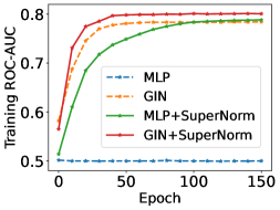
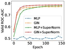
Figure 3. Learning curves of one-layer MLP, GIN, MLP + SuperNorm and GIN + SuperNorm on IMDB-BINARY dataset with various $k$-regular graphs.

Table 1. Experimental results on IMDB-BINARY dataset with various $k$-regular graphs. The best results under different backbones are highlighted with boldface.

	Normalization		Layers	ROC-AUC		LOSS
	Batchnorm	SuperNorm		Test Split	Valid Split	Test Split	Valid Split
MLP	$-$	$-$	1	56.66 $\pm$ 1.09	57.05 $\pm$ 0.81	0.6961	0.6961
	✓	$-$	1	56.86 $\pm$ 0.72	57.83 $\pm$ 0.84	0.6954	0.6954
	$-$	✓	1	78.13 $\pm$ 0.45	78.53 $\pm$ 0.50	0.5645	0.5589
GIN	$-$	$-$	1	77.40 $\pm$ 0.20	77.69 $\pm$ 0.13	0.5684	0.5658
	✓	$-$	1	77.71 $\pm$ 0.19	78.11 $\pm$ 0.10	0.5655	0.5593
	$-$	✓	1	78.22 $\pm$ 0.20	78.67 $\pm$ 0.16	0.5593	0.5588
GSN	$\checkmark$	$-$	1	77.50 $\pm$ 0.18	77.54 $\pm$ 0.16	0.5696	0.5688
GraphSNN	$\checkmark$	$-$	1	77.52 $\pm$ 0.16	77.61 $\pm$ 0.18	0.5691	0.5671
GIN	✓	$-$	4	78.41 $\pm$ 0.21	78.76 $\pm$ 0.17	0.5625	0.5590
	$-$	✓	4	79.52 $\pm$ 0.43	79.51 $\pm$ 0.34	0.5541	0.5523
GCN	✓	$-$	4	76.75 $\pm$ 1.31	76.96 $\pm$ 0.69	0.5755	0.5640
	$-$	✓	4	78.84 $\pm$ 0.91	79.01 $\pm$ 0.83	0.5594	0.5511
GAT	✓	$-$	4	75.10 $\pm$ 1.51	75.95 $\pm$ 1.27	0.5866	0.5852
	$-$	✓	4	78.73 $\pm$ 0.80	78.80 $\pm$ 0.76	0.5544	0.5451
GSN	$\checkmark$	$-$	4	78.90 $\pm$ 0.63	79.28 $\pm$ 0.70	0.5555	0.5543
	$-$	✓	4	79.32 $\pm$ 0.72	79.71 $\pm$ 0.59	0.5526	0.5524
GraphSNN	$\checkmark$	$-$	4	79.16 $\pm$ 0.67	79.35 $\pm$ 0.82	0.5541	0.5530
	$-$	✓	4	79.83 $\pm$ 0.75	79.87 $\pm$ 0.81	0.5521	0.5512

Baseline Methods. We compare our SuperNorm to various types of normalization baselines for GNNs, including BatchNorm (Ioffe and Szegedy, 2015), UnityNorm (Chen et al., 2022c), GraphNorm (Cai et al., 2021), ExpreNorm (Dwivedi et al., 2022a) for graph predictions, and GroupNorm (Zhou et al., 2020), PairNorm (Zhao and Akoglu, 2020), MeanNorm (Yang et al., 2020), NodeNorm (Zhou et al., 2021) for node, link predictions.

More details about datasets, baselines and hyperparameters are provided in the Appendix B. Furthermore, we provide some comparisons with regard to self-supervised leanring, larger datasets and runtime/memory consumption in the Appendix C.

(a) Accuracy

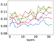
(b) Intra-class distance

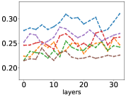
(c) Inter-class distance

Figure 4. Experimental results of vanilla GCN by setting layers from 2 to 32 with different normalization methods on Cora dataset.

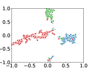
(a) SuperNorm,Layer=32

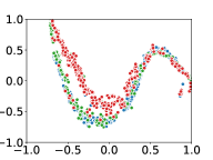
(b) GroupNorm,Layer=32

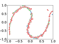
(c) BatchNorm,Layer=32

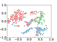
(d) NodeNorm,Layer=32

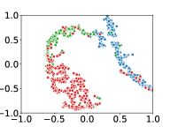
(e) MeanNorm,Layer=32

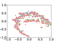
(f) PairNorm,Layer=32

Figure 5. The t-SNE visualization of node representations using GCN with different normalization methods on Cora dataset.

In the following experiments, we aim to answer the questions: (i) Can SuperNorm improve the expressivity for graph isomorphism test, especially go beyond 1-WL on $k$-regular graphs? (Section 4.1) (ii) Can SuperNorm help alleviate the over-smoothing issue? (Section 4.2) (iii) Can SuperNorm generalize to various graph tasks, including node, link and graph predictions? (Section 4.3)

4.1. Experimental Analysis on Graph Isomorphism Test

The IMDB-BINARY is a well-known graph isomorphism test dataset consisting of various $k$-regular graphs, which has become a common-used benchmark for evaluating the expressivity of GNNs. To make the training, valid and test sets follow the same distribution as possible, we adopt a hierarchical dataset splitting strategy based on the structural statistics of graphs (More detailed descriptions are provided in Appendix B.1). For graph isomorphism test, Graph Isomorphism Network (GIN) (Xu et al., 2019) is known to be as powerful as 1-WL. Notably, GIN consists a neighborhood aggregation operation and a multi-layer perception layer (MLP), and this motivates a comparison experiment: comparing a one-layer MLP+SuperNorm with one-layer GIN to directly demonstrate SuperNorm’s expressivity in distinguishing $k$-regular graphs.

As illustrated in Figure 3, the vanilla MLP cannot capture any structural information and perform poorly, while the proposed SuperNorm method successfully improve the performance of MLP and even exceeds the vanilla GIN. That is a direct explaination that SuperNorm can improve model’s expressivity in distinguishing graph structure. Furthermore, Table 1 provides the quantitative comparison results, where GSN (Bouritsas et al., 2022) and GraphSNN (Wijesinghe and Wang, 2022) are two recent popular methods realizing the higher expressivity than the 1-WL. From these comparison results, the performance of one-layer MLP with SuperNorm is better than that of one-layer GIN, GSN, and GraphSNN. Moreover, the commonly used GNNs equipped with SuperNorm, e.g., GCN and GAT, achieve higher ROC-AUC than GIN when the layer is set as 4. GIN with SuperNorm achieves better performance and even goes beyond the GSN and GraphSNN. Furthermore, SuperNorm can further enhance the expressivity of GSN and GraphSNN.

4.2. Experimental Analysis on the Over-smoothing Issue

To show the effectiveness of SuperNorm for alleviating the over-smoothing issue in GNNs, we provide the quantitative results by considering three metrics including accuracy, intra-class distance and inter-class distance. In details, we set layers from 2 to 32 with the step size as 2 by using vanilla GCN as backbone, and visualize the line chart in Figure 4(a)$\sim$4(c). Figure 4(a) shows the accuracy with regard to the number of GNNs’ layers, which directly demonstrates the superiority of SuperNorm when GNNs go deeper. In order to characterize the disentangling capability of different normalizations, we calculate the intra-class distance and inter-class distance with the number of layers increasing in Figure 4(b) and 4(c). As shown in these two figures, SuperNorm obtains lower intra-class distance and higher inter-class distance, which means that the proposed SuperNorm enjoys better disentangling ability.

Furthermore, we visualize the first three categories of Cora dataset in 2D space for a better illustration. We select PairNorm, NodeNorm, MeanNorm, GroupNorm and BatchNorm for comparison and set the number of layer as 32. Figure 5(a)$\sim$5(f) show the t-SNE visualization of different normalization techniques, and we can find that none of them suffer from the over-smoothing issue. However, SuperNorm can better distinguish different categories into different clusters, i.e., the other normalization methods may lead to the loss of discriminant information and make the representations indistinguishable.

Table 2. Experimental results of different normalization methods without any tricks for graph prediction tasks. We use GCN, GAT and GIN as the backbones and set the number of layers as 4, 16 and 32. The best results on each dataset are highlighted with boldface.

	Methods	ogbg-moltoxcast			ogbg-molhiv			ZINC
		$l=4$	$l=16$	$l=32$	$l=4$	$l=16$	$l=32$	$l=4$	$l=16$	$l=32$
GCN	NoNorm	61.13 $\pm$ 0.47	59.34 $\pm$ 0.78	56.08 $\pm$ 2.36	76.01 $\pm$ 0.92	71.90 $\pm$ 0.92	60.59 $\pm$ 2.55	0.643 $\pm$ 0.013	0.690 $\pm$ 0.014	0.748 $\pm$ 0.015
	GraphNorm	60.78 $\pm$ 1.03	53.75 $\pm$ 0.89	53.36 $\pm$ 1.08	75.59 $\pm$ 0.99	65.55 $\pm$ 4.15	66.49 $\pm$ 1.64	0.592 $\pm$ 0.009	0.655 $\pm$ 0.029	1.547 $\pm$ 0.001
	UnityNorm	63.86 $\pm$ 0.97	61.94 $\pm$ 1.10	59.18 $\pm$ 0.81	75.94 $\pm$ 0.93	72.14 $\pm$ 1.16	69.44 $\pm$ 1.30	0.552 $\pm$ 0.011	0.576 $\pm$ 0.011	0.650 $\pm$ 0.032
	ExpreNorm	64.97 $\pm$ 0.42	57.91 $\pm$ 0.55	57.82 $\pm$ 0.30	76.05 $\pm$ 0.95	76.75 $\pm$ 1.38	72.36 $\pm$ 0.50	0.564 $\pm$ 0.009	0.570 $\pm$ 0.015	0.646 $\pm$ 0.036
	BatchNorm	63.39 $\pm$ 1.03	59.73 $\pm$ 2.73	53.47 $\pm$ 1.36	76.11 $\pm$ 0.98	76.62 $\pm$ 1.79	74.21 $\pm$ 2.28	0.573 $\pm$ 0.016	0.611 $\pm$ 0.017	0.655 $\pm$ 0.025
	SuperNorm	67.12 $\pm$ 0.62	64.34 $\pm$ 0.72	63.22 $\pm$ 0.91	77.86 $\pm$ 1.28	77.70 $\pm$ 1.13	75.46 $\pm$ 1.96	0.483 $\pm$ 0.011	0.534 $\pm$ 0.010	0.531 $\pm$ 0.010
GAT	NoNorm	62.61 $\pm$ 0.45	50.84 $\pm$ 1.40	50.12 $\pm$ 0.37	76.71 $\pm$ 0.98	57.38 $\pm$ 5.58	50.64 $\pm$ 1.71	0.714 $\pm$ 0.043	1.541 $\pm$ 0.005	1.547 $\pm$ 0.004
	GraphNorm	60.53 $\pm$ 0.56	52.79 $\pm$ 0.83	53.22 $\pm$ 1.26	75.30 $\pm$ 1.21	73.86 $\pm$ 0.59	64.03 $\pm$ 5.23	0.576 $\pm$ 0.010	1.254 $\pm$ 0.324	1.537 $\pm$ 0.017
	UnityNorm	63.47 $\pm$ 0.67	58.76 $\pm$ 1.32	57.13 $\pm$ 1.72	75.91 $\pm$ 0.91	76.19 $\pm$ 0.63	75.46 $\pm$ 1.15	0.563 $\pm$ 0.012	0.621 $\pm$ 0.016	0.777 $\pm$ 0.015
	ExpreNorm	65.56 $\pm$ 0.55	57.65 $\pm$ 0.18	57.60 $\pm$ 0.15	76.99 $\pm$ 0.79	72.24 $\pm$ 0.69	72.56 $\pm$ 0.50	0.555 $\pm$ 0.009	0.562 $\pm$ 0.011	1.451 $\pm$ 0.001
	BatchNorm	63.31 $\pm$ 0.50	53.39 $\pm$ 1.85	53.24 $\pm$ 0.58	76.07 $\pm$ 0.79	76.87 $\pm$ 0.56	73.74 $\pm$ 3.85	0.585 $\pm$ 0.005	0.624 $\pm$ 0.017	0.643 $\pm$ 0.018
	SuperNorm	66.57 $\pm$ 1.00	63.68 $\pm$ 0.91	58.46 $\pm$ 1.05	77.42 $\pm$ 0.91	77.13 $\pm$ 1.01	76.81 $\pm$ 0.94	0.505 $\pm$ 0.010	0.511 $\pm$ 0.009	0.528 $\pm$ 0.013
GIN	NoNorm	62.19 $\pm$ 0.36	56.38 $\pm$ 2.25	54.83 $\pm$ 0.76	76.33 $\pm$ 1.05	69.70 $\pm$ 4.43	58.87 $\pm$ 4.06	0.496 $\pm$ 0.009	0.520 $\pm$ 0.010	1.069 $\pm$ 0.073
	GraphNorm	62.44 $\pm$ 0.91	54.95 $\pm$ 0.87	55.72 $\pm$ 1.07	76.55 $\pm$ 1.06	66.00 $\pm$ 1.65	67.01 $\pm$ 1.40	0.462 $\pm$ 0.012	1.203 $\pm$ 0.344	1.446 $\pm$ 0.008
	UnityNorm	64.15 $\pm$ 0.86	59.00 $\pm$ 1.03	55.98 $\pm$ 0.86	75.82 $\pm$ 1.45	68.43 $\pm$ 1.62	67.24 $\pm$ 1.56	0.442 $\pm$ 0.016	0.513 $\pm$ 0.011	1.150 $\pm$ 0.161
	ExpreNorm	65.98 $\pm$ 0.45	57.80 $\pm$ 1.75	56.56 $\pm$ 0.35	76.23 $\pm$ 1.16	69.97 $\pm$ 1.74	70.96 $\pm$ 1.71	0.438 $\pm$ 0.013	0.482 $\pm$ 0.013	1.157 $\pm$ 0.194
	BatchNorm	63.72 $\pm$ 0.57	58.67 $\pm$ 2.30	55.56 $\pm$ 0.79	76.62 $\pm$ 1.06	70.28 $\pm$ 2.83	66.82 $\pm$ 2.51	0.477 $\pm$ 0.012	0.516 $\pm$ 0.012	1.153 $\pm$ 0.201
	SuperNorm	66.86 $\pm$ 1.13	62.87 $\pm$ 0.83	57.53 $\pm$ 0.42	77.48 $\pm$ 0.98	73.13 $\pm$ 1.13	71.15 $\pm$ 1.33	0.430 $\pm$ 0.011	0.461 $\pm$ 0.009	0.921 $\pm$ 0.093

Table 3. The comparison results of different normalization methods without any tricks for node and link prediction tasks by using GCN and GraphSage as the backbone and setting the number of layers as 4, 16 and 32. The best results are highlighted with boldface.

	Settings	Pubmed			ogbn-proteins			ogbl-collab
		$l=4$	$l=16$	$l=32$	$l=4$	$l=16$	$l=32$	$l=4$	$l=16$	$l=32$
GCN	NoNorm	76.16 $\pm$ 1.23	54.67 $\pm$ 6.02	45.58 $\pm$ 2.70	69.16 $\pm$ 1.69	63.24 $\pm$ 0.65	63.15 $\pm$ 0.91	35.38 $\pm$ 0.50	22.11 $\pm$ 1.07	15.24 $\pm$ 1.10
	PairNorm	74.25 $\pm$ 2.34	56.24 $\pm$ 6.97	55.13 $\pm$ 4.30	69.28 $\pm$ 2.30	63.15 $\pm$ 0.35	63.00 $\pm$ 0.44	31.26 $\pm$ 2.82	23.22 $\pm$ 1.69	14.69 $\pm$ 1.25
	NodeNorm	76.02 $\pm$ 1.15	40.87 $\pm$ 1.23	41.18 $\pm$ 1.39	70.17 $\pm$ 1.46	63.50 $\pm$ 0.76	63.23 $\pm$ 0.88	27.48 $\pm$ 1.01	08.48 $\pm$ 0.68	08.28 $\pm$ 2.49
	MeanNorm	76.05 $\pm$ 0.80	73.40 $\pm$ 3.58	65.34 $\pm$ 6.62	69.14 $\pm$ 1.99	63.05 $\pm$ 0.38	62.40 $\pm$ 0.44	33.28 $\pm$ 1.43	22.56 $\pm$ 2.35	16.16 $\pm$ 1.22
	GroupNorm	76.19 $\pm$ 1.31	63.55 $\pm$ 5.37	54.84 $\pm$ 6.07	70.25 $\pm$ 2.26	62.74 $\pm$ 0.62	63.63 $\pm$ 1.41	35.28 $\pm$ 1.91	27.41 $\pm$ 2.36	20.27 $\pm$ 2.24
	BatchNorm	75.62 $\pm$ 0.69	48.88 $\pm$ 4.09	43.28 $\pm$ 3.07	69.96 $\pm$ 2.14	67.36 $\pm$ 1.63	63.86 $\pm$ 1.05	47.57 $\pm$ 0.27	26.14 $\pm$ 1.19	21.68 $\pm$ 1.74
	SuperNorm	77.11 $\pm$ 1.32	76.86 $\pm$ 1.46	66.41 $\pm$ 2.44	71.77 $\pm$ 1.37	68.41 $\pm$ 1.28	67.88 $\pm$ 2.50	50.95 $\pm$ 1.21	47.11 $\pm$ 0.98	45.22 $\pm$ 0.72
GraphSage	NoNorm	76.94 $\pm$ 0.88	40.65 $\pm$ 3.53	41.67 $\pm$ 2.07	66.05 $\pm$ 4.64	60.56 $\pm$ 0.57	60.47 $\pm$ 0.11	25.27 $\pm$ 2.37	02.08 $\pm$ 4.16	01.16 $\pm$ 0.78
	PairNorm	72.78 $\pm$ 1.66	53.02 $\pm$ 6.98	45.90 $\pm$ 4.26	62.29 $\pm$ 3.38	60.53 $\pm$ 0.27	60.32 $\pm$ 0.67	41.72 $\pm$ 1.25	16.88 $\pm$ 2.57	12.44 $\pm$ 2.66
	NodeNorm	77.22 $\pm$ 1.05	40.64 $\pm$ 1.66	40.64 $\pm$ 2.06	64.48 $\pm$ 3.64	62.63 $\pm$ 1.19	61.89 $\pm$ 1.35	19.74 $\pm$ 2.54	02.57 $\pm$ 0.51	02.62 $\pm$ 0.05
	MeanNorm	76.68 $\pm$ 0.91	58.70 $\pm$ 1.45	47.48 $\pm$ 6.86	63.69 $\pm$ 3.76	61.03 $\pm$ 6.50	52.06 $\pm$ 8.40	46.17 $\pm$ 2.77	21.54 $\pm$ 2.20	13.16 $\pm$ 1.40
	GroupNorm	76.83 $\pm$ 1.06	40.42 $\pm$ 4.59	43.49 $\pm$ 1.51	68.09 $\pm$ 2.61	61.58 $\pm$ 1.72	60.60 $\pm$ 0.17	45.43 $\pm$ 1.87	23.98 $\pm$ 2.45	15.43 $\pm$ 1.43
	BatchNorm	75.49 $\pm$ 1.72	45.11 $\pm$ 4.63	42.74 $\pm$ 3.46	63.75 $\pm$ 3.25	62.96 $\pm$ 3.03	61.54 $\pm$ 0.50	47.05 $\pm$ 1.43	23.01 $\pm$ 4.11	14.89 $\pm$ 1.58
	SuperNorm	77.21 $\pm$ 0.94	74.15 $\pm$ 2.42	73.45 $\pm$ 2.03	68.11 $\pm$ 1.53	67.14 $\pm$ 2.01	65.17 $\pm$ 2.43	51.98 $\pm$ 0.87	48.67 $\pm$ 0.71	48.41 $\pm$ 0.64

Table 4. The comparison results of different norms with empirical tricks on ogbg-molhiv and ZINC datasets.

	Methods	ogbg-molhiv	ZINC
GCN	NoNorm	77.21 $\pm$ 0.430	0.473 $\pm$ 0.006
	UnityNorm	77.56 $\pm$ 1.060	0.458 $\pm$ 0.009
	ExpreNorm	77.99 $\pm$ 0.545	0.436 $\pm$ 0.008
	GraphNorm	78.10 $\pm$ 1.115	0.396 $\pm$ 0.008
	BatchNorm	78.07 $\pm$ 0.782	0.398 $\pm$ 0.003
	SuperNorm	78.83 $\pm$ 0.615	0.369 $\pm$ 0.009

Table 5. The comparison results of different norms with empirical tricks on ogbn-proteins and ogbl-collab datasets.

	Methods	ogbn-proteins	ogbl-collab
GCN	PairNorm	69.84 $\pm$ 0.533	47.75 $\pm$ 0.190
	NodeNorm	72.53 $\pm$ 1.514	48.28 $\pm$ 1.100
	MeanNorm	71.09 $\pm$ 1.236	47.27 $\pm$ 0.849
	GroupNorm	73.17 $\pm$ 0.503	45.25 $\pm$ 1.206
	BatchNorm	72.39 $\pm$ 0.611	49.44 $\pm$ 0.750
	SuperNorm	73.68 $\pm$ 1.016	51.91 $\pm$ 0.874

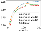
(a) Training ROC-AUC

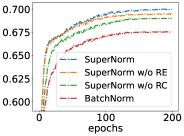
(b) Valid ROC-AUC

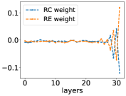
(c) Average weight in $w_{\texttt{RC}},w_{\texttt{RE}}$

Figure 6. Abalation study of the Representation Calibration (RC) and Representation Enhancement (RE) operations in SuperNorm on the ogbg-moltoxcast dataset. Here, we use GCN as the basic backbone to conduct the abalation study.

4.3. More Comparisons on the Other Six Datasets

For graph prediction task, we compare normalizations on ogbg-moltoxcast, ogbg-molhiv and ZINC, where ZINC is a graph regression dataset. For node and link property predictions we conduct experiments on one social network dataset (Pubmed), one protein-protein association network dataset (ogbn-proteins) and a collaboration network between authors (ogbl-collab). The details are as follow: Firstly, we adopt the vanilla GNN model without any tricks (e.g., residual connection, etc.). Accordingly to the mean results (w.r.t., 10 different seeds) shown in Table 2 and Table 5, we can conclude that SuperNorm generally improves the graph expressivity of GNNs for graph prediction task and help alleviate the over-smoothing issue with the increase of layers. Secondly, we perform empirical tricks in GNNs for a further comparison when generally obtaining better performances. The details of tricks on different datasets: (1) ogbg-molhiv: convolution with edge features, without input dropout, hidden dimension as 300, weight decay in $\{$5e-5, 1e-5$\}$, residual connection, GNN layers as 4. (2) ZINC: without input and hidden dropout, hidden dim as 145, residual connection, GNN layers as 4. (3) ogbn-proteins: without input and hidden dropout, hidden dim as 256, GNN layers as 2. (4) ogbl-collab: initial connection (Chen et al., 2020), GNN layers as 4. The results in Table 5 and Table  5 demonstrate that SuperNorm preserves the superiority in graph, node and link prediction tasks compared with other existent normalizations.

4.4. Ablation Study and Discussion

To explain the superior performance of SuperNorm, we perform extensive ablation studies to evaluate the contributions of its two key components, i.e., representation calibration (RC) and representation enhancement (RE) operations. Firstly, we show in Figure 6 the ablation performance of GCN on ogbg-moltoxcast. Figure 6(a) and 6(b) show the ROC-AUC results with regard to training epochs when the layer number is set to 4, which show that both RC and RE can improve the classification performance. Furthermore, by comparing these two figures, RC performs better than RE in terms of recognition results, which plugs at the beginning of BatchNorm with the graph instance-specific statistics embedded.

To further explore the significance of RC and RE at different layers, we compute the mean values of $w_{\texttt{RC}}$ and $w_{\texttt{RE}}$, which are visualized in Figure 6(c). As can be seen from the mean statistis of $w_{\texttt{RC}}$, $w_{\texttt{RE}}$ among 32 layers’ GCN, the absolute values of $w_{\texttt{RC}}$ and $w_{\texttt{RE}}$ become larger when the network goes deeper (especially in the last few layers), indicating that the structural information becomes more and more critical with the increase numbers of layers.

Table 6. The cost comparisons between BatchNorm and SuperNorm.

	runtime	parameter	memory
BatchNorm	15.2s/epoch	291.6K	2305M
SuperNorm	22.6s/epoch	293.2K	2347M

To evaluate the additional cost of RC and RE operations, we provide the runtime, parameter and memory comparison by using GCN ($l=4$) with BatchNorm and SuperNorm on ogbg-molhiv dataset. Here, we provide the cost of runtime and memory by performing the code on NVIDIA A40. The cost information is provided in Table 6.

Discussion. The main contribution of this work is to propose a more expressive normalization module, which can be plugged into any GNN architecture. Unlike existing normalization methods that are usually task-specific and also without substructure information, the proposed method explicitly considers the subgraph information to strengthen the graph expressivity across various graph tasks. In particular, for the task of graph classification, SuperNorm extends GNNs to be at least as powerful as 1-WL test for various non-isomorphic graphs. On the other hand, when the number of GNNs’ layers becomes larger, SuperNorm can prevent the output features of distant nodes to be too similar or indistinguishable, which helps alleviate the over-smoothing problem, and thus maintain better discriminative power for the node-relevant predictions.

5. Conclusion

In this paper, we introduce a higher-expressivity normalization architecture with subgraph-specific factor embedding to generally improve GNNs’ expressivities and representatives for various graph tasks. We first present a method to compute the subgraph-specific factor, which is proved to be exclusive for each non-isomorphic subgraph. Then, we empirically disentangle the standard normalization into two stages, i.e., centering $\&$ scaling (CS) and affine transformation (AT) operations, and elaborately develop two skillful strategies to embed the resulting powerful factor into CS and AT operations. Finally, we provide a theoretical analysis to support that SuperNorm can extend GNNs to be at least as powerful as 1-WL test in distinguishing non-isomorphic graphs and explain why it can help alleviate the over-smoothing issue when GNNs go deeper. Experimental results on eight popular benchmarks show that our method is highly efficient and can generally improve the performance of GNNs for various graph tasks.

6. Acknowledgement

This work is supported by the Science and Technology Project of SGCC: Hybrid enhancement intelligence with human-AI coordination and its application in reliability analysis of regional power system (5700-202217190A-1-1-ZN).

Appendix A Theorem Analysis

This section provides the corresponding proofs to support theorems in the main context.

A.1. Proof for Theorem 2

Theorem 1. GNNs are as powerful the as 1-WL test in distinguishing non-isomorphic graphs while any two different subgraphs $S_{v_{i}}$, $S_{v_{j}}$ are subtree-isomorphic (i.e., $S_{v_{i}}\simeq_{\texttt{subtree}}S_{v_{j}}$), or GNNs can map two different subgraphs into two different embeddings if and only if $S_{v_{i}}\not\simeq_{\texttt{subtree}}S_{v_{j}}$.

Proof.

We provide theoretical analysis by comparing the difference between the formulation of the message-passing GNNs and the 1-WL test, and detail as follow:

For graph representation learning using GNNs, node features in a graph are usually learned by following the neighborhood aggregation and representation updating schemes. In general, the formulation of the message-passing GNNs’ convolution can be represented as:

(13) $$\begin{split}\texttt{GNNs}:\,h_{v}^{(t)}=\mathcal{M}(h_{v}^{t-1},\mathcal{A}\{h_{u}^{t-1}|u\in\mathcal{N}(v)\}),\\ \end{split}$$

where $\mathcal{A}$ is the aggregation function, and $\mathcal{M}$ is a representation updating function. For a clear comparison with 1-WL test, we copy the formulation of 1-WL from Eq.(1) for comparing:

(14) $$\begin{split}\quad\texttt{1}\text{-}\texttt{WL}\,:\,h_{v}^{(t)}=\texttt{Hash}(h_{v}^{t-1},\mathcal{A}\{h_{u}^{t-1}|u\in\mathcal{N}(v)\}).\\ \end{split}$$

Let us compare the formulation of above Eq.(13) and Eq.(14), and we can find that the difference between the two equations is that the hash function Hash($\cdot$) and updating function $\mathcal{M}$($\cdot$). Here, the updating function $\mathcal{M}$ in GNNs is not always injective, so that may transform two different samples into the same representation, which is the main reason that GNNs are at most as powerful as the 1-WL test for graph isomorphic issues. To prove this theorem, we take the subtree-isomorphic issue (e.g., two node-induced subgraphs, $S_{v_{i}}$, $S_{v_{i}}$) for example and exemplify as follow:

• If $S_{v_{i}}\simeq_{\texttt{subtree}}S_{v_{j}}$, the simple neighborhood aggregation operation just concerns 1-hop information, resulting in both GNNs and 1-WL test can not distinguish these two substructures. In this case, GNNs are as powerful as 1-WL test in distinguishing non-isomorphic graphs.

• If $S_{v_{i}}\not\simeq_{\texttt{subtree}}S_{v_{j}}$ and $\mathcal{M}$ map two different substructures into different representations (i.e., $f(S_{v_{i}})\neq f(S_{v_{j}})$), which means that $\mathcal{M}$ distinguish these two substructures like Hash in 1-WL. In this case, GNNs are as powerful as 1-WL test in distinguishing non-isomorphic graphs.

• If $S_{v_{i}}\not\simeq_{\texttt{subtree}}S_{v_{j}}$, the neighborhood aggregation operation can obtain two different multisets. However, $\mathcal{M}$ may transform two different multisets into the same representation, which means that GNNs are not as powerful as 1-WL test in distinguishing non-isomorphic graphs.

To this end, we analyzed the existing conditions of GNNs as powerful as 1-WL. The first and second items are the statement of Theorem 2.

The proof is complete. ∎

A.2. Design of representation calibration factor

Here, we talk about the design of representation calibration factor $\text{M}_{\texttt{RC}}=\text{M}_{\texttt{SN}}\cdot\text{M}_{\mathcal{G}}$, which is a normalization for subgraph-specific factor $\text{M}_{\mathcal{G}}$. If we directly adopt the original weights, existing many unequal large values, it will make training oscillating. Thus, the normalization is essential for $\text{M}_{\mathcal{G}}$. However, if we just perform summation-normalization in an arbitrary graph (i.e., $\text{M}_{\texttt{SN}}$), it will not distinguish two graphs with the same nodes but different degrees, e.g., four graphs in Figure 7 where each weight will become 1/8. To this end, we design the above normalization technique to strengthen the subgraph power for the representation calibration.

Figure 7. The illustration of four $k$-regular graphs with the same nodes but different structures. When directly performing the summation-normalization operation on subgraph-specific, all weights will be equal to 1/8.

Appendix B Experimental Details

B.1. More Details of Benchmark Datasets and Baseline Methods

Benchmark Datasets. For the task of graph property prediction, we select IMDB-BINARY, ogbg-moltoxcast, ogbg-molhiv and ZINC datasets. The IMDB-BINARY is a $k$-regular dataset for binary classification task, which means that each node has a degree $k$. The ogbg-moltoxcast is collected for multi-task task, where the number of the tasks and classes are 617 and 37 respectively. The ogbg-molhiv is a molecule dataset that used for binary classification task, but the ouput dimension of the end-to-end GNNs is 1 because its metric is ROC-AUC. The ZINC is the real-world molecule dataset for the example reconstruction. In this paper, we follow the work in (Dwivedi et al., 2022a) to use ZINC for the task of graph regression. These graph prediction datasets are from (Morris et al., 2020; Hu et al., 2020; Irwin et al., 2012) respectively. For the node level prediction, we select four benchmark datasets including Cora, Pubmed and ogbn-proteins. The first two datasets are the social network and the last one is a protein-protein association network dataset. For the evalutation of link property prediction, we select ogbl-collab dataset in this paper. These node and link prediction datasets are from (Kipf and Welling, 2017; Hu et al., 2020) respectively. More details are provided in Table 7.

Experiment Setting. For different datasets, we provide more detailed statistics information in Table 7. The embedding dimension in each hidden layer on all datasets is set as 128. We optim the GNNs’ architectures using torch.optim.lr$\_$scheduler.ReduceLROnPlateau by setting patience step as $10$ or $15$ to reduce learning rate. The learning rate is $1e-3$ for graph classification, and $1e-2$ for node, link predictions. When the learning rate reduces to $1e-5$, the training will be terminated. More detailed statistics of experimental settings are provided in Table 8. Specially, we split the IMDB-BINARY dataset into train-vallid-test format using a hierarchical architecture. In details, we first segment this dataset according to the edge density information into ten set, i.e., the edge density $\in\{0.0-0.1\},\cup,\{0.1-0.2\}...,\{0.9-1.0\}$, and then sort the graphs using the average degree information. Finally, we select the samples in each segment using a fix step size as valid and test samples. The statistic information for splitting the valid and test set of Label-0 and Label-1 on IMDB-BINARY is provide in Table 9. By adopting this splitting scheme, distribution differences among train, valid and test sets are weakened (Experiment results show this contribution fact but without a theoretical basis now). To reproduce the comparison results using a single layer of MLP and GIN, the dropout is set to 0.0 and warming up the learning rate from 0.0 to $1e-3$ at the first 50 epoches. When layer is equal to 4, the doupout at the input layer is selected in $\{0.3,0.4,0.5\}$, and hidden layer is set to 0.5. To draw the Figure 3, we remove the warmup operation for learning rate. The $p$ in PloyHash is selected in $\{0.01-0.09\}$ with step as 0.01.

Table 7. The statistics of eight benchmark datasets.

Dataset Name	Dataset Type	Task Type	#Graphs	Avg.	Avg.
				#Nodes	#Edges
IMDB-BINARY	molecular	Graph classification	1,000	19.8	193.1
ogbg-toxcast	molecular	Graph classification	8,576	18.8	19.3
ogbg-molhiv	molecular	Graph classification	41,127	25.5	27.5
ZINC	molecular	Graph regression	10,000	23.2	49.8
Cora	social	Node classification	1	2,708	5,429
Pubmed	social	Node classification	1	19,717	44,338
ogbn-proteins	proteins	Node classification	1	132,534	39,561,252
ogbl-collab	social	Link classification	1	235,868	1,285,465

Table 8. The detailed settings on various graph tasks.

Name	Metrics	Edge Conv.	Layers	Learning Rate	Batch Size	InitDim.	HiDim.	Dropout
IMDB-BINARY	ROC-AUC	False	$1,$ $4$	$1e-3$	$32$	128	$128$	0.0, 0.5
ogbg-toxcast	ROC-AUC	False	$4,$ $16,$ $32$	$1e-3$	$128$	9	$128$	0.5
ogbg-molhiv	ROC-AUC	False	$4,$ $16,$ $32$	$1e-3$	$256$	9	$128$	0.5
ZINC	MAE	False	$4,$ $16,$ $32$	$1e-3$	$128$	1	$128$	0.5
Cora	Accuracy	False	$[0;2;32]$	$1e-2$	$--$	1433	$128$	0.5
Pubmed	Accuracy	False	$4,$ $16,$ $32$	$1e-2$	$--$	500	$128$	0.5
ogbn-proteins	ROC-AUC	False	$4,$ $16,$ $32$	$1e-2$	$--$	8	$128$	0.5
ogbl-collab	Hits@50	False	$4,$ $16,$ $32$	$1e-2$	$64\times 1024$	128	$128$	0.0

Table 9. The statistics for splitting IMDB-BINARY.

	0.0$-$0.1	0.1$-$0.2	0.2$-$0.3	0.3$-$0.4	0.4$-$0.5	0.5$-$0.6	0.6$-$0.7	0.7$-$0.8	0.8$-$0.9	0.9$-$1.0	1.0	Total Num.
Label-0	1	17	60	89	49	117	52	12	15	7	81	500
Label-1	0	22	81	145	58	97	30	8	1	0	58	500
2-12 Total Label	1	39	141	234	107	214	82	20	16	7	139	1000
Steps	-	9	8	7	6	5	4	3	2	2	6
2-12 Label-0 Sel.	0	2	14	28	16	46	30	8	14	6	26	190
Label-1 Sel.	0	4	20	40	18	38	14	4	0	0	18	156
2-12 Total Sel.	0	6	34	68	34	84	44	12	14	6	44	346

Appendix C Additional experiment

C.1. Comparisons on larger datasets

In this subsection, we conduct comparisons on significantly larger datasets such as ogbn-products and ogbn-mag, using the baselines of SIGN (Frasca et al., 2020) and LEGNN (Yu et al., 2022), which are reported in the ogb leaderboards.

Table 10. The comparative experiments on larger datasets.

Method	ogbn-products	Method	ogbn-mag
SIGN	0.8063 $\pm$ 0.0032	LEGNN	0.5289 $\pm$ 0.0011
SIGN with SuperNorm	0.8120 $\pm$ 0.0029	LEGNN with SuperNorm	0.5324 $\pm$ 0.0013

C.2. Comparisons in unsupervised/self-supervised settings

In this subsection, we conduct a comparison on MUTAG dataset by using InfoGraph (Sun et al., 2019) and MVGRL (Hassani and Khasahmadi, 2020) as baselines, which were selected in the DIG toolkit (Liu et al., 2021).

Table 11. The comparative experiments in unsupervised/self-supervised settings on MUTAG dataset.

Method	Acc.	Method	Acc.
InfoGraph	0.8930 $\pm$ 0.0514	MVGRL	0.8993 $\pm$ 0.0616
InfoGraph with SuperNorm	0.9037 $\pm$ 0.0607	MVGRL with SuperNorm	0.9068 $\pm$ 0.0671

C.3. Comparisons using more recent graph prediction methods

In this subsection, we follow the ogb leaderboards and provide additional comparison of recent graph prediction methods including DeepAUC (Yuan et al., 2021) and PAS+FPs (Wei et al., 2021) on the ogbg-molhiv dataset.

Table 12. The comparative experiments using recent graph prediction methods on ogbg-molhiv dataset.

Method	Test ROC-AUC	Method	Test ROC-AUC
DeepAUC	83.27 $\pm$ 0.61	PAS+FPs	83.98 $\pm$ 0.11
DeepAUC with SuperNorm	83.89 $\pm$ 0.57	PAS+FPs with SuperNorm	84.41 $\pm$ 0.15

C.4. Comparisons using a low number of GNNs layers

To further validate the performance in low-layer settings, we present comparative results on the Pubmed dataset by setting the number of layers as 2/3 for GCN and GraphSage.

Table 13. The comparative results on the Pubmed dataset.

Method	layer =2	layer =3	Method	layer =2	layer =3
GCN w/o Norm	76.27 $\pm$ 0.95	76.47 $\pm$ 0.89	GrapgSage w/o Norm	76.73 $\pm$ 0.69	76.98 $\pm$ 0.96
GCN with SuperNorm	76.65 $\pm$ 0.83	77.27 $\pm$ 1.03	GrapgSage with SuperNorm	77.08 $\pm$ 0.90	77.55 $\pm$ 1.08

C.5. Runtime and memory consumption

In this subsection, we provide the runtime and memory consumption. Firstly, we preprocess the subgraph-specific factors using Intel(R) Xeon(R) Gold 6342 CPU 2.80GHz and report the runtime consumption as follows:

Table 14. The runtime consumption on ten datasets.

IMDB-BINARY	ogbg-toxcast	ogbg-molhiv	ZINC	Cora	Pubmed	ogbn-proteins	ogbl-collab	ogbn-products	ogbl-collab
0.5 mins	0.7 mins	27 mins	1.4 mins	0.05 mins	0.3 mins	21.3 hours	18 hours	49.3 hours	33 hours

To some extent, the SuperNorm is not very proficient in handling large-scale dataset tasks by comprehensively considering the performance and the time consumption. For the specific task large scale dataset, it may be necessary to consider and design the normalization module from a new or specific perspective. In this paper, we design the normalization technique with regard to the perspective non-isomorphic test and over-smoothing issue, which may not be suitable for large scale processing.

Secondly, memory consumption for preprocessing is the data-loading consumption, as the model is not loaded. The additional consumption for each node is averaged 4Byte because the value of subgraph-specific factor is the type of float 32.

References

- (1)
- Alghamdi et al. (2021) Norah Alghamdi, Wennan Chang, Pengtao Dang, Xiaoyu Lu, Changlin Wan, Silpa Gampala, Zhi Huang, Jiashi Wang, Qin Ma, Yong Zang, et al. 2021. A graph neural network model to estimate cell-wise metabolic flux using single-cell RNA-seq data. Genome research 31, 10 (2021), 1867–1884.
- Bouritsas et al. (2022) Giorgos Bouritsas, Fabrizio Frasca, Stefanos P Zafeiriou, and Michael Bronstein. 2022. Improving graph neural network expressivity via subgraph isomorphism counting. IEEE Transactions on Pattern Analysis and Machine Intelligence (2022).
- Boyaci et al. (2021) Osman Boyaci, Mohammad Rasoul Narimani, Katherine R Davis, Muhammad Ismail, Thomas J Overbye, and Erchin Serpedin. 2021. Joint detection and localization of stealth false data injection attacks in smart grids using graph neural networks. IEEE Transactions on Smart Grid 13, 1 (2021), 807–819.
- Bui et al. (2021) Khac-Hoai Nam Bui, Jiho Cho, and Hongsuk Yi. 2021. Spatial-temporal graph neural network for traffic forecasting: An overview and open research issues. Applied Intelligence (2021), 1–12.
- Cai et al. (2021) Tianle Cai, Shengjie Luo, Keyulu Xu, Di He, Tie-yan Liu, and Liwei Wang. 2021. Graphnorm: A principled approach to accelerating graph neural network training. In International Conference on Machine Learning. PMLR, 1204–1215.
- Cappart et al. (2021) Quentin Cappart, Didier Chételat, Elias Khalil, Andrea Lodi, Christopher Morris, and Petar Veličković. 2021. Combinatorial optimization and reasoning with graph neural networks. arXiv preprint arXiv:2102.09544 (2021).
- Chen et al. (2022a) Kaixuan Chen, Shunyu Liu, Na Yu, Rong Yan, Quan Zhang, Jie Song, Zunlei Feng, and Mingli Song. 2022a. Distribution-Aware Graph Representation Learning for Transient Stability Assessment of Power System. International Joint Conference on Neural Networks (IJCNN) (2022).
- Chen et al. (2022b) Kaixuan Chen, Jie Song, Shunyu Liu, Na Yu, Zunlei Feng, Gengshi Han, and Mingli Song. 2022b. Distribution Knowledge Embedding for Graph Pooling. IEEE Transactions on Knowledge and Data Engineering (2022).
- Chen et al. (2020) Ming Chen, Zhewei Wei, Zengfeng Huang, Bolin Ding, and Yaliang Li. 2020. Simple and deep graph convolutional networks. In International Conference on Machine Learning. 1725–1735.
- Chen et al. (2022d) Tianlong Chen, Kaixiong Zhou, Keyu Duan, Wenqing Zheng, Peihao Wang, Xia Hu, and Zhangyang Wang. 2022d. Bag of tricks for training deeper graph neural networks: A comprehensive benchmark study. IEEE Transactions on Pattern Analysis and Machine Intelligence (2022).
- Chen et al. (2022c) Yihao Chen, Xin Tang, Xianbiao Qi, Chun-Guang Li, and Rong Xiao. 2022c. Learning graph normalization for graph neural networks. Neurocomputing 493 (2022), 613–625.
- Chen et al. (2023) Ziheng Chen, Tianyang Xu, Xiao-Jun Wu, Zhiwu Huang, and Josef Kittler. 2023. Riemannian Local Mechanism for SPD Neural Networks. In AAAI.
- Dwivedi et al. (2022a) Vijay Prakash Dwivedi, Chaitanya K Joshi, Thomas Laurent, Yoshua Bengio, and Xavier Bresson. 2022a. Benchmarking graph neural networks. arXiv preprint arXiv:2003.00982 (2022).
- Dwivedi et al. (2022b) Vijay Prakash Dwivedi, Anh Tuan Luu, Thomas Laurent, Yoshua Bengio, and Xavier Bresson. 2022b. Graph Neural Networks with Learnable Structural and Positional Representations. In International Conference on Learning Representations.
- Frasca et al. (2020) Fabrizio Frasca, Emanuele Rossi, Davide Eynard, Ben Chamberlain, Michael Bronstein, and Federico Monti. 2020. Sign: Scalable inception graph neural networks. arXiv preprint arXiv:2004.11198 (2020).
- Gupta et al. (2021) Atika Gupta, Priya Matta, and Bhasker Pant. 2021. Graph neural network: Current state of Art, challenges and applications. Materials Today: Proceedings 46 (2021), 10927–10932.
- Gusfield (1997) Dan Gusfield. 1997. Algorithms on stings, trees, and sequences: Computer science and computational biology. Acm Sigact News 28, 4 (1997), 41–60.
- Han et al. (2022) Xiaotian Han, Zhimeng Jiang, Ninghao Liu, and Xia Hu. 2022. G-mixup: Graph data augmentation for graph classification. In International Conference on Machine Learning. PMLR, 8230–8248.
- Hassani and Khasahmadi (2020) Kaveh Hassani and Amir Hosein Khasahmadi. 2020. Contrastive multi-view representation learning on graphs. In International conference on machine learning. 4116–4126.
- He et al. (2016) Kaiming He, Xiangyu Zhang, Shaoqing Ren, and Jian Sun. 2016. Deep residual learning for image recognition. In Proceedings of the IEEE conference on computer vision and pattern recognition. 770–778.
- Hu et al. (2020) Weihua Hu, Matthias Fey, Marinka Zitnik, Yuxiao Dong, Hongyu Ren, Bowen Liu, Michele Catasta, and Jure Leskovec. 2020. Open graph benchmark: Datasets for machine learning on graphs. Advances in neural information processing systems 33 (2020), 22118–22133.
- Ioffe and Szegedy (2015) Sergey Ioffe and Christian Szegedy. 2015. Batch normalization: Accelerating deep network training by reducing internal covariate shift. In International conference on machine learning. 448–456.
- Irwin et al. (2012) John J Irwin, Teague Sterling, Michael M Mysinger, Erin S Bolstad, and Ryan G Coleman. 2012. ZINC: a free tool to discover chemistry for biology. Journal of chemical information and modeling 52, 7 (2012), 1757–1768.
- Jing et al. (2022) Yongcheng Jing, Yining Mao, Yiding Yang, Yibing Zhan, Mingli Song, Xinchao Wang, and Dacheng Tao. 2022. Learning graph neural networks for image style transfer. In Computer Vision–ECCV 2022: 17th European Conference, Tel Aviv, Israel, October 23–27, 2022, Proceedings, Part VII. Springer, 111–128.
- Jing et al. (2023a) Yongcheng Jing, Xinchao Wang, and Dacheng Tao. 2023a. Segment anything in non-euclidean domains: Challenges and opportunities. arXiv preprint arXiv:2304.11595 (2023).
- Jing et al. (2021a) Yongcheng Jing, Yiding Yang, Xinchao Wang, Mingli Song, and Dacheng Tao. 2021a. Amalgamating knowledge from heterogeneous graph neural networks. In Proceedings of the IEEE/CVF conference on computer vision and pattern recognition. 15709–15718.
- Jing et al. (2021b) Yongcheng Jing, Yiding Yang, Xinchao Wang, Mingli Song, and Dacheng Tao. 2021b. Meta-aggregator: learning to aggregate for 1-bit graph neural networks. In Proceedings of the IEEE/CVF International Conference on Computer Vision. 5301–5310.
- Jing et al. (2023b) Yongcheng Jing, Chongbin Yuan, Li Ju, Yiding Yang, Xinchao Wang, and Dacheng Tao. 2023b. Deep Graph Reprogramming. In CVPR.
- Karp and Rabin (1987) Richard M Karp and Michael O Rabin. 1987. Efficient randomized pattern-matching algorithms. IBM journal of research and development 31, 2 (1987), 249–260.
- Kipf and Welling (2017) Thomas N Kipf and Max Welling. 2017. Semi-supervised classification with graph convolutional networks. International Conference on Learning Representation (2017).
- Leiserson et al. (1994) Charles Eric Leiserson, Ronald L Rivest, Thomas H Cormen, and Clifford Stein. 1994. Introduction to algorithms. Vol. 3. MIT press Cambridge, MA, USA.
- Li et al. (2023) Hui Li, Tianyang Xu, Xiao-Jun Wu, Jiwen Lu, and Josef Kittler. 2023. LRRNet: A novel representation learning guided fusion framework for infrared and visible images. IEEE Transactions on Pattern Analysis and Machine Intelligence (2023). DOI: 10.1109/TPAMI.2023.3268209.
- Li et al. (2022) Jiachen Li, Siheng Chen, Xiaoyong Pan, Ye Yuan, and Hong-Bin Shen. 2022. Cell clustering for spatial transcriptomics data with graph neural networks. Nature Computational Science 2, 6 (2022), 399–408.
- Li and Zhu (2021) Mengzhang Li and Zhanxing Zhu. 2021. Spatial-temporal fusion graph neural networks for traffic flow forecasting. In Proceedings of the AAAI conference on artificial intelligence. 4189–4196.
- Li et al. (2018) Qimai Li, Zhichao Han, and Xiao-Ming Wu. 2018. Deeper Insights Into Graph Convolutional Networks for Semi-Supervised Learning. In Proceedings of the Thirty-Second AAAI Conference on Artificial Intelligence, Sheila A. McIlraith and Kilian Q. Weinberger (Eds.). 3538–3545.
- Liu et al. (2021) Meng Liu, Youzhi Luo, Limei Wang, Yaochen Xie, Hao Yuan, Shurui Gui, Haiyang Yu, Zhao Xu, Jingtun Zhang, Yi Liu, Keqiang Yan, Haoran Liu, Cong Fu, Bora M Oztekin, Xuan Zhang, and Shuiwang Ji. 2021. DIG: A Turnkey Library for Diving into Graph Deep Learning Research. Journal of Machine Learning Research 22, 240 (2021), 1–9. http://jmlr.org/papers/v22/21-0343.html
- Liu et al. (2022) Songhua Liu, Kai Wang, Xingyi Yang, Jingwen Ye, and Xinchao Wang. 2022. Dataset distillation via factorization. In NeurIPS.
- Ma et al. (2023) Xinyin Ma, Gongfan Fang, and Xinchao Wang. 2023. LLM-Pruner: On the Structural Pruning of Large Language Models. arXiv:2305.11627 [cs.CL]
- Morris et al. (2020) Christopher Morris, Nils M Kriege, Franka Bause, Kristian Kersting, Petra Mutzel, and Marion Neumann. 2020. Tudataset: A collection of benchmark datasets for learning with graphs. arXiv preprint arXiv:2007.08663 (2020).
- Poole (2014) David Poole. 2014. Linear algebra: A modern introduction. Cengage Learning.
- Schuetz et al. (2022) Martin JA Schuetz, J Kyle Brubaker, and Helmut G Katzgraber. 2022. Combinatorial optimization with physics-inspired graph neural networks. Nature Machine Intelligence 4, 4 (2022), 367–377.
- Sun et al. (2019) Fan-Yun Sun, Jordan Hoffmann, Vikas Verma, and Jian Tang. 2019. Infograph: Unsupervised and semi-supervised graph-level representation learning via mutual information maximization. arXiv preprint arXiv:1908.01000 (2019).
- Tavakoli et al. (2022) Mohammadamin Tavakoli, Aaron Mood, David Van Vranken, and Pierre Baldi. 2022. Quantum mechanics and machine learning synergies: graph attention neural networks to predict chemical reactivity. Journal of Chemical Information and Modeling 62, 9 (2022), 2121–2132.
- Veličković et al. (2018) Petar Veličković, Guillem Cucurull, Arantxa Casanova, Adriana Romero, Pietro Lio, and Yoshua Bengio. 2018. Graph attention networks. International Conference on Learning Representation (2018).
- Wang et al. (2021) Jinsong Wang, Fan Zhang, Huanan Liu, Jianyong Ding, and Ciwei Gao. 2021. Interruptible load scheduling model based on an improved chicken swarm optimization algorithm. CSEE Journal of Power and Energy Systems 7, 2 (2021), 232–240.
- Wang et al. (2019) Minjie Wang, Da Zheng, Zihao Ye, Quan Gan, Mufei Li, Xiang Song, Jinjing Zhou, Chao Ma, Lingfan Yu, Yu Gai, Tianjun Xiao, Tong He, George Karypis, Jinyang Li, and Zheng Zhang. 2019. Deep Graph Library: A Graph-Centric, Highly-Performant Package for Graph Neural Networks. arXiv preprint arXiv:1909.01315 (2019).
- Wang et al. (2023) Rui Wang, Xiao-Jun Wu, Tianyang Xu, Cong Hu, and Josef Kittler. 2023. U-SPDNet: An SPD manifold learning-based neural network for visual classification. Neural Networks 161 (2023), 382–396.
- Wei et al. (2021) Lanning Wei, Huan Zhao, Quanming Yao, and Zhiqiang He. 2021. Pooling architecture search for graph classification. In Proceedings of the 30th ACM International Conference on Information & Knowledge Management. 2091–2100.
- Weisfeiler and Leman (1968) Boris Weisfeiler and Andrei Leman. 1968. The reduction of a graph to canonical form and the algebra which appears therein. NTI, Series 2, 9 (1968), 12–16.
- Wijesinghe and Wang (2022) Asiri Wijesinghe and Qing Wang. 2022. A New Perspective on” How Graph Neural Networks Go Beyond Weisfeiler-Lehman?”. In International Conference on Learning Representations.
- Xu et al. (2019) Keyulu Xu, Weihua Hu, Jure Leskovec, and Stefanie Jegelka. 2019. How Powerful are Graph Neural Networks?. In International Conference on Learning Representations.
- Xu et al. (2023a) Tianyang Xu, Zhenhua Feng, Xiao-Jun Wu, and Josef Kittler. 2023a. Toward Robust Visual Object Tracking With Independent Target-Agnostic Detection and Effective Siamese Cross-Task Interaction. IEEE Transactions on Image Processing 32 (2023), 1541–1554.
- Xu et al. (2023b) Tianyang Xu, Xue-Feng Zhu, and Xiao-Jun Wu. 2023b. Learning spatio-temporal discriminative model for affine subspace based visual object tracking. Visual Intelligence 1, 1 (2023), 4.
- Yang et al. (2020) Chaoqi Yang, Ruijie Wang, Shuochao Yao, Shengzhong Liu, and Tarek Abdelzaher. 2020. Revisiting over-smoothing in deep GCNs. arXiv preprint arXiv:2003.13663 (2020).
- Yang et al. (2022b) Fan Yang, Zenan Ling, Yuhang Zhang, Xing He, Qian Ai, and Robert C Qiu. 2022b. Event Detection, Localization, and Classification Based on Semi-Supervised Learning in Power Grids. IEEE Transactions on Power Systems (2022).
- Yang et al. (2022a) Xingyi Yang, Zhou Daquan, Songhua Liu, Jingwen Ye, and Xinchao Wang. 2022a. Deep model reassembly. In NeurIPS.
- Yang et al. (2022c) Xingyi Yang, Jingwen Ye, and Xinchao Wang. 2022c. Factorizing knowledge in neural networks. In ECCV.
- Ye et al. (2023) Shanding Ye, Zhe Yin, Yongjian Fu, Hu Lin, and Zhijie Pan. 2023. A multi-granularity semisupervised active learning for point cloud semantic segmentation. Neural Computing and Applications (2023), 1–17.
- Yu et al. (2022) Le Yu, Leilei Sun, Bowen Du, Tongyu Zhu, and Weifeng Lv. 2022. Label-Enhanced Graph Neural Network for Semi-supervised Node Classification. IEEE Transactions on Knowledge and Data Engineering (2022).
- Yu et al. (2023) Ruonan Yu, Songhua Liu, and Xinchao Wang. 2023. Dataset Distillation: A Comprehensive Review. arXiv preprint arXiv:2301.07014 (2023).
- Yuan et al. (2021) Zhuoning Yuan, Yan Yan, Milan Sonka, and Tianbao Yang. 2021. Large-scale robust deep auc maximization: A new surrogate loss and empirical studies on medical image classification. In Proceedings of the IEEE/CVF International Conference on Computer Vision. 3040–3049.
- Zhao and Akoglu (2020) Lingxiao Zhao and Leman Akoglu. 2020. PairNorm: Tackling Oversmoothing in GNNs. In International Conference on Learning Representations, ICLR.
- Zhong et al. (2022) Zipeng Zhong, Jie Song, Zunlei Feng, Tiantao Liu, Lingxiang Jia, Shaolun Yao, Min Wu, Tingjun Hou, and Mingli Song. 2022. Root-aligned SMILES: a tight representation for chemical reaction prediction. Chemical Science 13, 31 (2022), 9023–9034.
- Zhou et al. (2021) Kuangqi Zhou, Yanfei Dong, Kaixin Wang, Wee Sun Lee, Bryan Hooi, Huan Xu, and Jiashi Feng. 2021. Understanding and Resolving Performance Degradation in Deep Graph Convolutional Networks. In ACM International Conference on Information and Knowledge Management CIKM. 2728–2737.
- Zhou et al. (2020) Kaixiong Zhou, Xiao Huang, Yuening Li, Daochen Zha, Rui Chen, and Xia Hu. 2020. Towards deeper graph neural networks with differentiable group normalization. Advances in neural information processing systems 33 (2020), 4917–4928.