Element-wise and Recursive Solutions for the Power Spectral Density
of Biological Stochastic Dynamical Systems at Fixed Points

Abstract

Stochasticity plays a central role in nearly every biological process, and the noise power spectral density (PSD) is a critical tool for understanding variability and information processing in living systems. In steady-state, many such processes can be described by stochastic linear time-invariant (LTI) systems driven by Gaussian white noise, whose PSD is a complex rational function of the frequency that can be concisely expressed in terms of their Jacobian, dispersion, and diffusion matrices, fully defining the statistical properties of the system’s dynamics at steady-state. Here, we arrive at compact element-wise solutions of the rational function coefficients for the auto- and cross-spectrum that enable the explicit analytical computation of the PSD in dimensions $n=2,3,4$. We further present a recursive Leverrier-Faddeev-type algorithm for the exact computation of the rational function coefficients. Crucially, both solutions are free of matrix inverses. We illustrate our element-wise and recursive solutions by considering the stochastic dynamics of neural systems models, namely Fitzhugh-Nagumo ($n=2$), Hindmarsh-Rose ($n=3$), Wilson-Cowan ($n=4$), and the Stabilized Supralinear Network ($n=22$), as well as an evolutionary game-theoretic model with mutations ($n=5,31$).

Unlike in an abstract painting by Mondrian [1], the world is not made of perfect forms. Rather, we are surrounded by imperfect, yet regular patterns emerging from the randomness of microscopic processes that collectively give rise to statistically predictable phenomena. A point in case is the derivation of the diffusion equation from the random (Brownian) motion of microscopic particles [2, 3]. This is but one example of the many processes that can be recapitulated in terms of ordinary differential equations driven by random processes, known as stochastic differential equations (SDEs). For instance, the effect of thermal fluctuations on synaptic conductance (linked to the stochastic opening of voltage-gated ion channels) and on the voltage of an electrical circuit (Johnson’s noise), or the fluctuations of a neuron’s membrane potential driven by stochastic spike arrival, can all be modeled as SDEs. Alternatively, SDEs are commonly adopted to model processes for which the exact dynamics are not known, and it is thus appropriate to express the model in terms of random variables encoding our uncertainty about the state of the system. Examples are the trajectory of an aircraft as modeled by navigation systems, or the evolution of stock prices subject to market fluctuations [4].

Among stochastic models, linear time-invariant (LTI) SDEs play a special role because (i) they are amenable to analytical treatment and (ii) the linear response of many nonlinear systems (e.g., around a fixed point of the dynamics) can be reduced to LTI SDEs. To make this point explicit, let us consider a non-linear autonomous dynamical system driven by additive white noise with finite variance, namely

$$\mathrm{d}\mathbf{x}=\mathbf{f}(\mathbf{x})\mathrm{d}t+\mathbf{L}\mathrm{d}\mathbf{W}$$ (1)

where $\textbf{x}\in\mathbb{R}^{n}$ is the state vector, $\textbf{f}:\mathbb{R}^{n}\to\mathbb{R}^{n}$ is a nonlinear drift function encoding the deterministic dynamics, $\mathbf{L}\in\mathbb{R}^{n\times m}$ is the dispersion matrix defining how noise enters the system, and $\mathrm{d}\mathbf{W}\in\mathbb{R}^{m}$ is a vector of mutually independent Gaussian increments satisfying $\mathbb{E}[\mathrm{d}\textbf{W}\mathrm{d}\textbf{W}^{\top}]=\mathbf{D}\mathrm{d}t$ where $\mathbf{D}$ is the diffusion matrix (or spectral density matrix) with entries $D_{ij}=\delta_{ij}\sigma_{i}^{2}$, where $\delta_{ij}$ is the Kronecker delta [4].

We are interested in the power spectral density (PSD) of the system’s response, $\mathbf{x}(t)$, near a stable fixed point, $\mathbf{x}_{0}$, so we proceed by linearizing the drift function about this point, yielding the following LTI system

$$\mathrm{d}\mathbf{x}=\mathbf{J}\mathbf{x}\mathrm{d}t+\mathbf{L}\mathrm{d}\mathbf{W}$$ (2)

where we have redefined $\mathbf{x}(t)\equiv\mathbf{x}(t)-\mathbf{x}_{0}$ such that $\mathbf{x}(t_{0})=\mathbf{0}$, and $\textbf{J}=\left.|\mathrm{d}\mathbf{f}/\mathrm{d}\mathbf{x}\right|_{\mathbf{x}_{0}}\in\mathbb{R}^{n\times n}$ is the Jacobian evaluated at the fixed point, that we take to be Hurwitz (real part of all eigenvalues less than zero) to assure stability. The solution to this linear SDE is given by the stochastic integral $\mathbf{x}(t)=\int_{-\infty}^{t}e^{\mathbf{J}(t-s)}\mathbf{L}\mathrm{d}\mathbf{W}(s)$ which is a zero-mean stationary process with covariance $\bf{\mathbfcal{R}}(\tau)$.

The PSD of this stochastic process is known to be expressed in terms of the following matrix product (see [5] and Supplemental Material),

$$\mathbfcal{S}_{\mathbf{x}}(\omega)=(\dot{\iota}\omega\mathbf{I}+\mathbf{J})^{-1}\,\mathbf{L}\,\mathbf{D}\,\mathbf{L}^{\top}(-\dot{\iota}\omega\mathbf{I}+\mathbf{J})^{-\top}$$ (3)

For the sake of brevity, from now on we refer to $\mathbfcal{S}_{\mathbf{x}}(\omega)$ as $\mathbfcal{S}(\omega)$, whose $i,j^{\text{th}}$ entry is denoted $\mathcal{S}^{ij}(\omega)$. $\mathbfcal{S}(\omega)$ is a product of the spectral factors (the transfer function matrix) of the dynamical system and can be expressed as a rational function, [6, 7] & Appendix A, of the following form,

$$\begin{split}\mathbfcal{S}(\omega)&=\frac{\mathbf{P}(\omega)+\dot{\iota}\omega\mathbf{P}^{\prime}(\omega)}{Q(\omega)}\\ &=\frac{\sum\limits_{\alpha=0}^{n-1}\mathbf{P}_{\alpha}\omega^{2\alpha}+\dot{\iota}\omega\sum\limits_{\alpha=0}^{n-2}\mathbf{P}_{\alpha}^{\prime}\omega^{2\alpha}}{\sum\limits_{\alpha=0}^{n}q_{\alpha}\omega^{2\alpha}}\end{split}$$ (4)

and the corresponding elements are of the form,

$$\mathcal{S}^{ij}(\omega)=\frac{P^{ij}(\omega)+\dot{\iota}\delta_{ij}\omega P^{ij\prime}(\omega)}{Q(\omega)}$$ (5)

where $P^{ij}(\omega)=\sum_{\alpha=0}^{n-1}p^{ij}_{\alpha}\omega^{2\alpha}$, $P^{ij\prime}(\omega)=\sum_{\alpha=0}^{n-2}p^{ij\prime}_{\alpha}\omega^{2\alpha}$ and $Q(\omega)=\sum_{\alpha=0}^{n}q_{\alpha}\omega^{2\alpha}$ are even powered polynomials with real coefficients.

In this work, we derive closed-form expressions for the individual coefficients of the rational function of a given element of $\mathbfcal{S}(\omega)$, i.e., $\mathcal{S}^{ij}(\omega)$. Thus, in Sec. II.3 we provide the formulae for the auto-spectrum of $2$, $3$, and $4$-dimensional systems expressed in terms of elementary trace operations applied to the submatrices of $\mathbf{J}$. The element-wise solutions for the auto- and cross-spectrum of a generic $n$-dimensional system are presented in the Supplemental Material, and they can be obtained directly in symbolic form through our software (see section VI). In Sec. III, we also derive a recursive algorithm to calculate the coefficient matrices $\mathbf{P}_{\alpha}$ and $\mathbf{P}_{\alpha}^{\prime}$ and the coefficients of the denominator, $q_{\alpha}$. We follow an approach similar to the one adopted by Hou [8] to derive the Leverrier-Faddeev (LF) method, which is a recursive approach to find the characteristic polynomial of a matrix in $O(n^{4})$ operations, where $n$ is the dimensionality of the system [9, 10]. Note that unlike Eq. 3, our solutions are free of matrix inverses, which is numerically advantageous when the system is ill-conditioned. Finally, in Sec. IV we apply our solutions to several stochastic nonlinear models from neuroscience and evolutionary biology, providing model-specific solutions for the auto-spectrum when appropriate. In practice, readers seeking analytical expressions for the auto-spectrum of specific models (e.g., Fitzhugh-Nagumo [11, 12, 13], or Hindmarsh-Rose [14]), can refer directly to Sec. I and IV.

I Preliminary examples

Before presenting the general solutions, it is instructive to review concrete 1- and 2-dimensional cases that are commonly encountered in the literature, for which we can derive the coefficients analytically with little effort, without resorting to our sophisticated solutions. To this end, let us consider the simplest and most common case: the auto-spectrum of an LTI system with mutually independent additive noise (i.e., $\textbf{L}=\textbf{I}$). For the $d=1$ case, also known as the Ornstein-Uhlenbeck process, we have

$$\mathrm{d}x=-\tau_{r}^{-1}x\mathrm{d}t+\mathrm{d}W$$ (6)

with $\mathrm{d}W^{2}=\sigma^{2}\mathrm{d}t$. It can be seen from Eq. 3 that

$$\mathcal{S}(\omega)=\frac{\sigma^{2}}{\tau_{r}^{-2}+\omega^{2}}$$ (7)

so that the coefficients in Eq. 5 are $p^{11}_{0}=\sigma^{2}$, $q_{0}=\tau_{r}^{-2}$ and $q_{1}=1$.

A slightly more sophisticated example is the stochastic Fitzhugh-Nagumo model [11, 12, 13], which amounts to a simplification of the Hodgkin-Huxley equations for action potential generation [16]. We simulate the dynamical evolution of a neuron’s membrane potential in response to an input current by the following set of SDEs

$$\begin{split}\frac{\mathrm{d}v}{\mathrm{d}t}&=\biggl{(}v-\frac{v^{3}}{3}-w+I\biggr{)}+h_{1}(v)\eta_{1}\\ \frac{\mathrm{d}w}{\mathrm{d}t}&=\epsilon(v+\alpha-\beta w)+h_{2}(w)\eta_{2}\end{split}$$ (8)

Here, $v$ represents the difference between the membrane potential and the resting potential, $w$ is the variable associated with the recovery of the ion channels after generation of an action potential, and $I$ is the external current input. The parameters $\alpha$ and $\beta$ are related to the activation threshold of the fast sodium channel and the inactivation threshold of the slow potassium channels, respectively. $\epsilon\ll 1$ sets the time scale for the evolution of the activity, making the dynamics of $v$ much faster than those of $w$. In the subthreshold regime, the fixed point, $(v_{e},w_{e})$, can be found analytically as a function of the parameters of the model and the input current (details in Supplemental Material). The stochasticity in $v$ and $w$ is represented by two uncorrelated Gaussian white noise sources, $\eta_{1}$ and $\eta_{2}$, with a standard deviation of 1. We consider the case of multiplicative noise which is realized by setting $h_{1}(v)$ and $h_{2}(w)$ proportional to the respective function variables. Specifically, we set $h_{1}(v)=0$ and $h_{2}(w)=\sigma w$. We choose the variance of the noise small enough that we are always in the vicinity of the fixed point. Then, upon linearizing Eq. 8 around the fixed point, $(v_{e},w_{e})$, we arrive at the following LTI SDEs,

$$\begin{bmatrix}\dot{v}\\ \dot{w}\end{bmatrix}=\begin{bmatrix}1-v_{e}^{2}&-1\\ \epsilon&-\beta\epsilon\end{bmatrix}\begin{bmatrix}v-v_{e}\\ w-w_{e}\end{bmatrix}+\sigma\begin{bmatrix}0&0\\ 0&w_{e}\end{bmatrix}\begin{bmatrix}\eta_{1}\\ \eta_{2}\end{bmatrix}$$ (9)

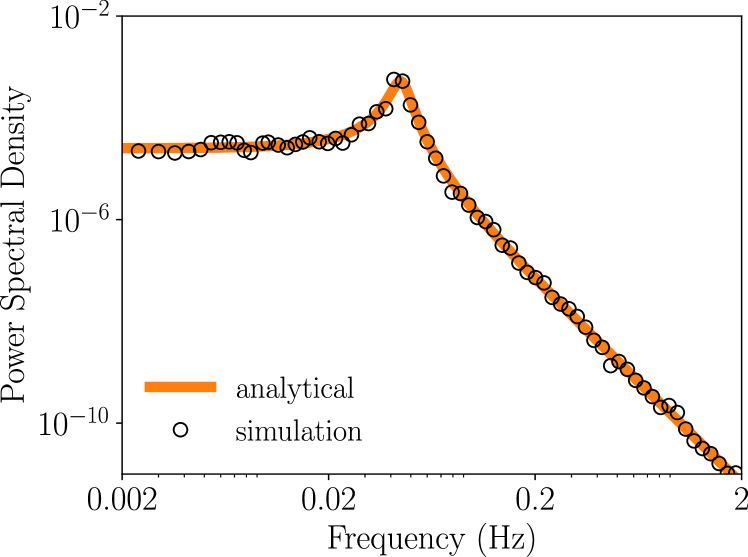
Figure 1: Power spectral density of the membrane potential for the Fitzhugh-Nagumo model. A comparison of the PSD of the membrane potential ($v$) calculated via simulation and the analytical rational function solution. The parameters used to simulate the system are $I=0.265$, $\alpha=0.7$, $\beta=0.75$ and $\epsilon=0.08$ that yields a fixed point solution $v_{e}=-1.00125$, $w_{e}=-0.401665$. Here, we plot the auto-spectrum for the case of multiplicative noise, i.e., $h_{1}(v)=0$ and $h_{2}(w)=\sigma w$, where $\sigma=0.001$.

Plugging the Jacobian and noise matrices into Eq. 3, we obtain the PSD of the membrane potential, $v$, as

$$\mathcal{S}_{v}(\omega) =w_{e}^{2}\sigma^{2}{\Big{/}}\left[(\epsilon+(v_{e}^{2}-1)\beta\epsilon)^{2}\right.$$ (10)

$$+\left.((v_{e}^{2}-1)^{2}-2\epsilon+\beta^{2}\epsilon^{2})\omega^{2}+\omega^{4}\right]$$

so that in Eq. 5 we have $p^{11}_{0}=w_{e}^{2}\sigma^{2}$, $p^{11}_{1}=0$, $q_{0}=(\epsilon+(v_{e}^{2}-1)\beta\epsilon)^{2}$, $q_{1}=((v_{e}^{2}-1)^{2}-2\epsilon+\beta^{2}\epsilon^{2})$ and $q_{2}=1$.

We verify the accuracy of this solution, Eq. 10, by comparison with the PSD obtained numerically by simulating the nonlinear model, Eq. 8, with multiplicative noise, and find excellent agreement as shown in Fig. 1.

This laborious approach works well for systems with dimensions $n=1,2$, but it becomes infeasible in higher dimensions. This is due to the multiplication of inverses of two matrices with complex entries, $(\dot{\iota}\omega\mathbf{I}+\mathbf{J})^{-1}$ and $(-\dot{\iota}\omega\mathbf{I}+\mathbf{J})^{-\top}$.

II Element-wise solution

We now present element-wise solutions for the auto-spectrum of 2, 3, and 4-dimensional systems. The general $n$-dimensional solutions for both auto- and cross-spectrum can be found in the Supplemental Material alongside their derivations. This method relies on expressing the rational function expression of Eq. 3 in terms of elementary matrix operations on submatrices of the Jacobian, $\mathbf{J}$. Although this approach requires roughly $O(n^{4}\log n)$ (Supplemental Material, Fig. S2), operations for each element of the PSD matrix, i.e., $O(n^{6}\log n)$ total, it is particularly valuable to arrive at analytical closed-form solutions for the auto- or cross-spectra of specific dynamical variables, yielding greater insight into the dependence of the power spectral density on the model’s functional form and its parameters. For simplicity, we consider the auto-spectrum of an LTI system driven by uncorrelated white noise (see Supplemental Material for the most general case of correlated noise and/or the cross-spectrum).

We start by noting that the denominator in Eq. 5 is independent of the type of noise driving the system, and it can be written as an even-powered expansion in $\omega$ with real coefficients. Similarly, the numerator of the auto-spectrum is an even-powered expansion in $\omega$ with real coefficients, but they depend directly on how the noise is added via the dispersion matrix, $\mathbf{L}$, whose elements we denote $l_{ij}$. For the particular case of independent noise, i.e., $l_{ij}=0$ for $i\neq j$, the coefficient of $\omega^{2\alpha}$ in the numerator of the rational function for the $i^{th}$ variable takes the simplified form,

$$p^{ii}_{\alpha}=\sigma^{2}_{i}\,l_{i}^{2}\,d^{\alpha}(\mathbf{O}_{ii})+\sum_{\begin{subarray}{c}j=1\\ j\neq i\end{subarray}}^{n}\sigma^{2}_{j}\,l_{j}^{2}\,f^{\alpha}(\mathbf{O}_{ji},\mathbf{e}_{\min(i,j)})$$ (11)

where $d^{\alpha}(\mathbf{O}_{ii})$ and $f^{\alpha}(\mathbf{O}_{ji})$ are functions of the Jacobian submatrices, $\mathbf{O}_{ij}$, defined according to the algorithm in Fig. 2. The functions themselves can be expressed in terms of Bell polynomials [17], and are defined in Supplemental Material (Sec. 5). $\mathbf{e}_{\beta}\in\{0,1\}^{n-1\times 1}$ is the standard unit vector equal to 1 at index $\beta=\min(i,j)$ and 0 everywhere else. $\sigma_{i}^{2}\equiv\sigma_{ii}^{2}$ is the $i$-th diagonal entry of the noise matrix $\mathbf{D}$, and, since $\mathbf{L}$ is diagonal, we also use the notation $l_{i}\equiv l_{ii}$.

Here, we only provide the solution for the auto-spectrum of the first variable, i.e., $i=1$. This solution can be generalized for any variable $i\neq 1$, as shown in Supplemental Material. Alternatively, one can simply interchange the rows and columns of the LTI system so that the variable of interest appears at index $i=1$, and directly use the solution reported in this section.

Since the coefficients of the denominator are the same for all dimensions, $n$, we define them first,

$$\begin{split}q_{n-4}&=\frac{1}{24}\bigg{[}\operatorname{Tr}^{4}{\left(\mathbf{J}^{2}\right)}-6\operatorname{Tr}^{2}{\left(\mathbf{J}^{2}\right)}\operatorname{Tr}{\left(\mathbf{J}^{4}\right)}\\ &+8\operatorname{Tr}{\left(\mathbf{J}^{2}\right)}\operatorname{Tr}{\left(\mathbf{J}^{6}\right)}+3\operatorname{Tr}^{2}{\left(\mathbf{J}^{4}\right)}-6\operatorname{Tr}{\left(\mathbf{J}^{8}\right)}\biggr{]}\\ q_{n-3}&=\frac{\operatorname{Tr}^{3}{\left(\mathbf{J}^{2}\right)}-3\operatorname{Tr}{\left(\mathbf{J}^{2}\right)}\operatorname{Tr}{\left(\mathbf{J}^{4}\right)}+2\operatorname{Tr}{\left(\mathbf{J}^{6}\right)}}{6}\\ q_{n-2}&=\frac{\operatorname{Tr}^{2}{\left(\mathbf{J}^{2}\right)}-\operatorname{Tr}{\left(\mathbf{J}^{4}\right)}}{2}\\ q_{n-1}&=\operatorname{Tr}{\left(\mathbf{J}^{2}\right)}\\ q_{n}&=1\end{split}$$ (12)

Note that for each $n$ we will only need to consider the coefficients $q_{\alpha}$ with $\alpha\geq 0$.

II.1 2-D solution

For a 2D system, we can write the auto-spectrum of the first variable as,

$$\mathcal{S}^{11}(\omega)=\frac{p_{0}+p_{1}\omega^{2}}{q_{0}+q_{1}\omega^{2}+q_{2}\omega^{4}}$$ (13)

where the coefficients of the numerator are given by the equations

$$\begin{split}p_{0}&=l_{1}^{2}\sigma_{1}^{2}\operatorname{Tr}(\mathbf{O}_{11}^{2})+l_{2}^{2}\sigma_{2}^{2}\operatorname{Tr}(\mathbf{O}_{21}^{2})\\ p_{1}&=l_{1}^{2}\sigma_{1}^{2}\end{split}$$ (14)

Here, the matrices $\mathbf{O}_{11}=[a_{22}$] and $\mathbf{O}_{21}=[a_{12}]$ are found from the 2D Jacobian using the algorithm summarized in Fig. 2 (n.b., we denote $a_{ij}$ the $i,j^{\text{th}}$ entry of the Jacobian). The coefficients of the denominator are given by the last three entries of Eq. 12.

II.2 3-D solution

For a 3D system, the auto-spectrum of the first variable takes the form,

$$\mathcal{S}^{11}(\omega)=\frac{p_{0}+p_{1}\omega^{2}+p_{2}\omega^{4}}{q_{0}+q_{1}\omega^{2}+q_{2}\omega^{4}+q_{3}\omega^{6}}$$ (15)

where the coefficients of the numerator are given by the equations

$$\begin{split}p_{0}=&\frac{1}{2}\biggl{[}l_{1}^{2}\sigma_{1}^{2}\bigl{(}\operatorname{Tr}^{2}{(\mathbf{O}_{11}^{2})}-\operatorname{Tr}{(\mathbf{O}_{11}^{4})}\bigr{)}+\sum_{j=2}^{3}l_{j}^{2}\sigma_{j}^{2}\bigl{(}\operatorname{Tr}^{2}{({\mathbf{O}^{\prime}_{j1}}^{2})}\\ &-\operatorname{Tr}{({\mathbf{O}^{\prime}_{j1}}^{4})}+\operatorname{Tr}^{2}{(\mathbf{O}_{j1}^{2})}-\operatorname{Tr}{(\mathbf{O}_{j1}^{4})}\bigr{)}\biggr{]}\\ p_{1}=&l_{1}^{2}\sigma_{1}^{2}\operatorname{Tr}{(\mathbf{O}_{11}^{2})}+\sum_{j=2}^{3}l_{j}^{2}\sigma_{j}^{2}\bigl{(}-2\operatorname{Tr}{(\mathbf{O}^{\prime}_{j1})}\operatorname{Tr}{(\mathbf{O}_{j1})}\\ &+\operatorname{Tr}{({\mathbf{O}^{\prime}_{j1}}^{2})}+\operatorname{Tr}^{2}{(\mathbf{O}_{j1})}\bigr{)}\\ p_{2}=&l_{1}^{2}\sigma_{1}^{2}\end{split}$$ (16)

Here, the matrices $\mathbf{O}_{11}$, $\mathbf{O}_{21}$ and $\mathbf{O}_{31}$ are found from the 3D Jacobian matrix using the algorithm summarized in Fig. 2. Furthermore, the matrices $\mathbf{O}^{\prime}_{ij}$ are found by excluding the $k^{th}$ row and column from the corresponding $\mathbf{O}_{ij}$ matrix, where $k=\min(i,j)$. Since we are interested in the spectrum of the first variable ($j=1$), $k=\min(i,1)=1$. Thus, $\mathbf{O}^{\prime}_{21}$ and $\mathbf{O}^{\prime}_{31}$ are found by removing the first row and column from the matrices $\mathbf{O}_{21}$ and $\mathbf{O}_{31}$, respectively. The coefficients of the denominator are given by the last four entries of Eq. 12.

If the variance of the noise is the same for all the variables, i.e., $l_{1}^{2}\sigma_{1}^{2}=l_{2}^{2}\sigma_{2}^{2}=l_{3}^{2}\sigma_{3}^{2}=\sigma^{2}$, we can further simplify the coefficients of the numerator, which become

$$\begin{split}p_{0}&=\sigma^{2}\mathrm{det}(\mathbf{A}^{\top}\mathbf{A})\\ p_{1}&=\sigma^{2}\operatorname{Tr}(\mathbf{A}_{1}^{\top}\mathbf{A}_{1}+\mathbf{A}_{2}^{2})\\ p_{2}&=\sigma^{2}\end{split}$$ (17)

where, $\mathbf{A}\in\mathbb{R}^{3\times 2}$ is the submatrix of $\mathbf{J}$ obtained by removing its first column. Then, $\mathbf{A}_{1}\in\mathbb{R}^{1\times 2}$ is the submatrix obtained by isolating the first row of $\mathbf{A}$, and $\mathbf{A}_{2}\in\mathbb{R}^{2\times 2}$ is the submatrix obtained by removing the first row of $\mathbf{A}$.

II.3 4-D solution

For a 4D system, the auto-spectrum of the first variable becomes

$$\mathcal{S}^{11}(\omega)=\frac{p_{0}+p_{1}\omega^{2}+p_{2}\omega^{4}+p_{3}\omega^{6}}{q_{0}+q_{1}\omega^{2}+q_{2}\omega^{4}+q_{3}\omega^{6}+q_{4}\omega^{8}}$$ (18)

where the coefficients of the numerator are given by Eq. 19. Here, the matrices $\mathbf{O}_{11}$, $\mathbf{O}_{21}$, $\mathbf{O}_{31}$ and $\mathbf{O}_{41}$ are found from the 4D Jacobian matrix using the algorithm summarized in Fig. 2. Using an argument similar to the 3D case, $\mathbf{O}^{\prime}_{21}$, $\mathbf{O}^{\prime}_{31}$ and $\mathbf{O}^{\prime}_{41}$ can be found by removing the first row and column from the matrices $\mathbf{O}_{21}$, $\mathbf{O}_{31}$ and $\mathbf{O}_{41}$, respectively. The coefficients of the denominator are given by Eq. 12.

$$\begin{split}p_{0}=&\frac{1}{6}\biggl{[}l_{1}^{2}\sigma_{1}^{2}\bigl{(}\operatorname{Tr}^{3}{(\mathbf{O}_{11}^{2})}-3\operatorname{Tr}{(\mathbf{O}_{11}^{2})}\operatorname{Tr}{(\mathbf{O}_{11}^{4})}+2\operatorname{Tr}{(\mathbf{O}_{11}^{6})}\bigr{)}+\sum_{j=2}^{4}l_{j}^{2}\sigma_{j}^{2}\biggl{(}\operatorname{Tr}^{3}{({\mathbf{O}^{\prime}_{j1}}^{2})}-3\operatorname{Tr}{({\mathbf{O}^{\prime}_{j1}}^{2})}\operatorname{Tr}{({\mathbf{O}^{\prime}_{j1}}^{4})}\\ &\qquad+2\operatorname{Tr}{({\mathbf{O}^{\prime}_{j1}}^{6})}+\operatorname{Tr}^{3}{(\mathbf{O}_{j1}^{2})}-3\operatorname{Tr}{(\mathbf{O}_{j1}^{2})}\operatorname{Tr}{(\mathbf{O}_{j1}^{4})}+2\operatorname{Tr}{(\mathbf{O}_{j1}^{6})}\biggr{)}\biggr{]}\\ p_{1}=&\frac{1}{6}\biggl{[}3l_{1}^{2}\sigma_{1}^{2}\bigl{(}\operatorname{Tr}^{2}{(\mathbf{O}_{11}^{2})}-\operatorname{Tr}{(\mathbf{O}_{11}^{4})}\bigr{)}+\sum_{j=2}^{4}l_{j}^{2}\sigma_{j}^{2}\biggl{(}-3\bigl{(}\operatorname{Tr}^{2}{(\mathbf{O}^{\prime}_{j1})}-\operatorname{Tr}{({\mathbf{O}^{\prime}_{j1}}^{2})}\bigr{)}\bigl{(}\operatorname{Tr}^{2}{(\mathbf{O}_{j1})}-\operatorname{Tr}{(\mathbf{O}_{j1}^{2})}\bigr{)}+3\operatorname{Tr}^{2}{({\mathbf{O}^{\prime}_{j1}}^{2})}\\ &+2\operatorname{Tr}{(\mathbf{O}^{\prime}_{j1})}\bigl{(}\operatorname{Tr}^{3}{(\mathbf{O}_{j1})}-3\operatorname{Tr}{(\mathbf{O}_{j1})}\operatorname{Tr}{(\mathbf{O}_{j1}^{2})}+2\operatorname{Tr}{(\mathbf{O}_{j1}^{3})}\bigr{)}-3\operatorname{Tr}{({\mathbf{O}^{\prime}_{j1}}^{4})}+3\operatorname{Tr}^{2}{(\mathbf{O}_{j1}^{2})}-3\operatorname{Tr}{(\mathbf{O}_{j1}^{4})}\biggr{)}\biggr{]}\\ p_{2}=&l_{1}^{2}\sigma_{1}^{2}\operatorname{Tr}{(\mathbf{O}_{11}^{2})}+\sum_{j=2}^{4}l_{j}^{2}\sigma_{j}^{2}\bigl{(}\operatorname{Tr}^{2}{(\mathbf{O}^{\prime}_{j1})}+\operatorname{Tr}^{2}{(\mathbf{O}_{j1})}-2\operatorname{Tr}{(\mathbf{O}^{\prime}_{j1})}\operatorname{Tr}{(\mathbf{O}_{j1})}\bigr{)}\\ p_{3}=&l_{1}^{2}\sigma_{1}^{2}\end{split}$$ (19)

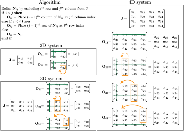
Figure 2: Definitions of $\mathbf{O}_{ij}$ matrices. We show the algorithm to generate the $\mathbf{O}_{ij}$ matrices with examples for the 2, 3 and 4D systems. To find $\mathbf{O}_{ij}$, we have to first find the excluded matrix by removing the $i^{th}$ row and $j^{th}$ column (denoted by green lines) from the Jacobian matrix and then perform the row/column change operations, denoted by orange arrows.

III Recursive solution

We derive an alternative approach to computing the polynomial coefficients of the auto- and cross-spectrum based on a recursive algorithm. By this method, we can obtain coefficients for all entries of the power spectral matrix simultaneously in $O(n^{4})$ operations (Supplemental Material, Fig. S1). To make our solution compact, we denote the noise covariance matrix $\mathbf{C}\equiv\mathbf{L}\,\mathbf{D}\,\mathbf{L}^{\top}$. We specify the algorithm in the following theorem and provide a proof in Supplemental Material. Note that the algorithm can alternatively be derived by leveraging the Barnett-Leverrier recursive formula [18].

Theorem III.1.

The noise power spectral density matrix of an LTI system is a complex-valued rational function of the form

$$\begin{split}\mathbfcal{S}(\omega)&=(\dot{\iota}\omega\mathbf{I}+\mathbf{J})^{-1}\,\mathbf{C}\,(-\dot{\iota}\omega\mathbf{I}+\mathbf{J})^{-\top}\\ &=\frac{\sum\limits_{\alpha=0}^{n-1}\mathbf{P}_{\alpha}\omega^{2\alpha}+\dot{\iota}\omega\sum\limits_{\alpha=0}^{n-2}\mathbf{P}_{\alpha}^{\prime}\omega^{2\alpha}}{\sum\limits_{\alpha=0}^{n}q_{\alpha}\omega^{2\alpha}}\end{split}$$

The numerator’s matrix coefficients are given by the recursive equations,

$$\begin{split}\mathbf{P}_{\alpha-1}^{\prime}&=\mathbf{J}\mathbf{P}_{\alpha}-\mathbf{P}_{\alpha}\mathbf{J}^{\top}-\mathbf{J}\mathbf{P}_{\alpha}^{\prime}\mathbf{J}^{\top}\\ \mathbf{P}_{\alpha-1}&=q_{\alpha}\mathbf{C}+\mathbf{P}_{\alpha-1}^{\prime}\mathbf{J}^{\top}-\mathbf{J}\mathbf{P}_{\alpha-1}^{\prime}-\mathbf{J}\mathbf{P}_{\alpha}\mathbf{J}^{\top}\end{split}$$ (20)

for $\alpha\in\{1,\dots,n\}$, starting from $\alpha=n$ with $\mathbf{P}_{n}=\mathbf{P}_{n}^{\prime}=\mathbf{0}$. The scalar coefficients of the denominator can be recursively calculated using,

$$\begin{split}q_{\alpha}=\frac{1}{n-\alpha}\left[\operatorname{Tr}\left(\mathbf{J}\mathbf{Q}_{\alpha-1}^{\prime}\right)+\operatorname{Tr}\left(\mathbf{J}\mathbf{Q}_{\alpha}\mathbf{J}^{\top}\right)\right]\end{split}$$ (21)

if $\alpha<n$, and $q_{n}=1$. The coefficients $\mathbf{Q}_{\alpha-1}^{\prime}$ and $\mathbf{Q}_{\alpha}$ are given in turn by the recursive equations,

$$\begin{split}\mathbf{Q}_{\alpha-1}^{\prime}&=\mathbf{J}\mathbf{Q}_{\alpha}-\mathbf{Q}_{\alpha}\mathbf{J}^{\top}-\mathbf{J}\mathbf{Q}_{\alpha}^{\prime}\mathbf{J}^{\top}\\ \mathbf{Q}_{\alpha-1}&=q_{\alpha}\mathbf{I}+\mathbf{Q}_{\alpha-1}^{\prime}\mathbf{J}^{\top}-\mathbf{J}\mathbf{Q}_{\alpha-1}^{\prime}-\mathbf{J}\mathbf{Q}_{\alpha}\mathbf{J}^{\top}\end{split}$$ (22)

for $\alpha\in\{0,1,\dots,n\}$, starting from $\alpha=n$ with $\mathbf{Q}_{n}=\mathbf{Q}_{n}^{\prime}=\mathbf{0}$ and $\mathbf{Q}_{-1}=\mathbf{Q}_{-1}^{\prime}=\mathbf{0}$.

Note that Eq. 22 is the same as Eq. 20 for $\mathbf{C}=\mathbf{I}$, and that the $\mathbf{P}_{\alpha}^{\prime}$ ($\mathbf{Q}_{\alpha}^{\prime}$) matrices are anti-symmetric, whereas the $\mathbf{P}_{\alpha}$ ($\mathbf{Q}_{\alpha}$) matrices are symmetric.

IV Applications

We now apply the rational function solutions of sections II.3 and III to compute the power spectra of a range of nonlinear models exhibiting fixed point solutions and, where appropriate, we provide analytical closed form expressions. We consider four models: (i) The stochastic Hindmarsh-Rose model simulating the subthreshold activity of a neuron subject to an input current [14, 19]; (ii) a 4D Wilson-Cowan model simulating the activity of excitatory and inhibitory neuronal populations in the cortex [20, 21]; (iii) the stochastic Stabilized Supralinear Network (SSN) model [22, 23], which is a neural circuit model for the sensory cortex approximating divisive normalization [24, 25]; (iv) an evolutionary game-theoretic model which involves a population of agents playing a generalized version of the rock-paper-scissors game in $n$ dimensions [26].

IV.1 Hindmarsh-Rose

Hindmarsh-Rose [14, 19] is a phenomenological 3D neuron model that can be considered a simplification of the Hodgkin-Huxley equations [16] or a generalization of the Fitzhugh-Nagumo model [11, 13]. We consider a stochastic version of the model based on the implementation by Storace et al. [19]. The system of SDEs defining the model is given by

$$\begin{split}\frac{\mathrm{d}x}{\mathrm{d}t}&=y-x^{3}+bx^{2}+I-z+\sigma\eta_{1}\\ \frac{\mathrm{d}y}{\mathrm{d}t}&=1-5x^{2}-y\\ \frac{\mathrm{d}z}{\mathrm{d}t}&=\mu\bigl{(}s(x-x_{rest})-z\bigr{)}\end{split}$$ (23)

Here, $x$ represents the membrane potential of the neuron, $y$ is a recovery variable, and $z$ is a slow adaptation variable. $I$ represents the synaptic current input to the neuron; $\mu\ll 1$ controls the relative timescales between the fast subsystem $(x,y)$ and the slow $z$ variable; $x_{rest}$ is the resting state of the membrane potential of the neuron; $s$ governs adaptation, and $b$ controls the transition of the activity to different dynamical states (quiescent, spiking, regular bursting, irregular bursting and so on) [19]. We add Gaussian white noise, $\sigma\eta_{1}$, with standard deviation $\sigma$, to the membrane potential and choose the model parameters so that the system is in a quiescent (subthreshold) state with a single stable equilibrium, namely $I=5.5$, $b=0.5$, $\mu=0.01$, $x_{rest}=-1.6$, $s=4$ and $\sigma=0.001$ .

Since the system is in a quiescent state, it exhibits a single fixed-point solution. Assuming that the deterministic steady-state is given by the triplet $(x_{e},y_{e},z_{e})$, we can linearize the system about the fixed point and write Eq. 23 as the LTI system

$$\begin{bmatrix}\dot{x}\\ \dot{y}\\ \dot{z}\end{bmatrix}=\begin{bmatrix}2bx_{e}-3x_{e}^{2}&1&-1\\ -10x_{e}&-1&0\\ \mu s&0&-\mu\\ \end{bmatrix}\begin{bmatrix}x-x_{e}\\ y-y_{e}\\ z-z_{e}\end{bmatrix}+\begin{bmatrix}\sigma\eta_{1}\\ 0\\ 0\end{bmatrix}$$ (24)

To show how our element-wise solution leads to a closed-form expression for the power spectrum of the membrane potential, we use the general analytical solution for a 3D system given by Eq. 15,

$$\mathcal{S}_{x}(\omega)=\frac{Z(\omega)}{Q(\omega)}=\frac{p_{0}+p_{1}\omega^{2}+p_{2}\omega^{4}}{q_{0}+q_{1}\omega^{2}+q_{2}\omega^{4}+q_{3}\omega^{6}}.$$

From the application of Eq. 12, we obtain the coefficients of the denominator, $Q(\omega)$, as

$$\begin{split}q_{0}=&\mu^{2}(x_{e}(3x_{e}-2b+10)+s)^{2}\\ q_{1}=&\mu^{2}\left((x_{e}(3x_{e}-2b)+s)^{2}-20x_{e}+1\right)\\ &+x_{e}^{2}(3x_{e}-2b+10)^{2}-2\mu s+20\mu sx_{e}\\ q_{2}=&x_{e}\left(x_{e}(3x_{e}-2b)^{2}-20\right)+\mu^{2}-2\mu s+1\\ q_{3}=&1\end{split}$$ (25)

Similarly, the coefficients of the numerator, $Z(\omega)$, can be found from Eq. 16: using the fact that $\sigma_{1}=\sigma_{2}=\sigma_{3}=\sigma$, $l_{1}=1$, and $l_{2}=l_{3}=0$, we obtain

$$\begin{split}p_{0}=&\frac{1}{2}\sigma^{2}\bigl{(}\operatorname{Tr}^{2}{(\mathbf{O}_{11}^{2})}-\operatorname{Tr}{(\mathbf{O}_{11}^{4})})\\ p_{1}=&\sigma^{2}\operatorname{Tr}{(\mathbf{O}_{11}^{2})}\\ p_{2}=&\sigma^{2}\end{split}$$ (26)

Now, plugging $\mathbf{O}_{11}$ given by

$$\mathbf{O}_{11}=\begin{bmatrix}-1&0\\ 0&-\mu\end{bmatrix}$$ (27)

into the equation above, yields the polynomial expansion of the numerator as,

$$Z(\omega)=\mu^{2}\sigma^{2}+\left(\mu^{2}+1\right)\sigma^{2}\omega^{2}+\sigma^{2}\omega^{4}$$ (28)

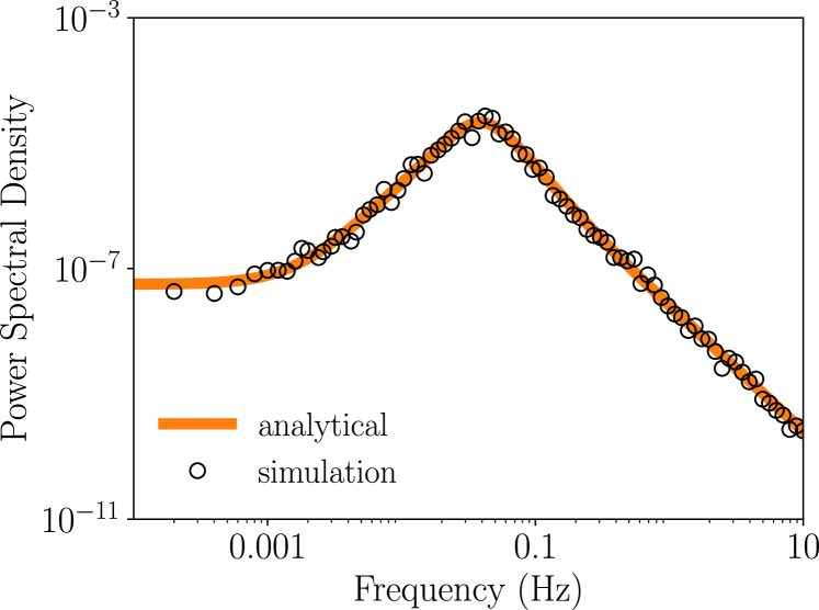
Figure 3: Power spectrum of the Hindmarsh-Rose model. The power spectral density of the membrane potential $x$, is calculated via simulation and our analytical (element-wise) solution. We use the following parameters to simulate the model: $I=5.5$, $b=0.5$, $\mu=0.01$, $x_{rest}=-1.6$, and $s=4$. We consider the case of additive Gaussian white noise with standard deviation $\sigma=0.001$.

We simulate the 3D system and verify that the simulated spectrum matches with the analytical element-wise solution we just derived, shown in Fig. 3. Furthermore, we calculate and plot the power spectral density for the membrane potential $x$, and the absolute cross-power spectral density and coherence between the fast variables $x$ and $y$, using Welchfls method [28] (simulation), the recursive and element-wise rational function solutions, and the “matrix solution” given by Eq. 3 (n.b., this relies on a numerical inverse). We confirm that all the solutions match across the entire range of frequencies, see Supplemental Material, Fig. S3.

IV.2 Wilson-Cowan model

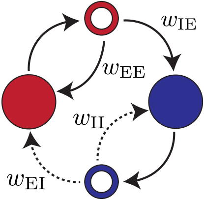
Figure 4: Wilson-Cowan 4D model. The mean-field circuit consists of 4 variables modeling excitatory activity (solid red), inhibitory activity (solid blue), excitatory synaptic activity (hollow red), and inhibitory synaptic activity (hollow blue). The solid and dashed arrows indicate excitatory and inhibitory connections, respectively. $w_{\mathrm{ij}}$, with $i,j\in\{\mathrm{E},\mathrm{I}\}$, represents the weight associated with the connections from $\mathrm{j}$ to $\mathrm{i}$.

The Wilson-Cowan model is a rate-based model that simulates the activity of Excitatory (E) and Inhibitory (I) populations of neurons and has been shown to exhibit gamma oscillations (30-120 Hz) for an appropriate choice of time constants [20]. Specifically, we consider a stochastic 4-dimensional version of the model introduced by Keeley et al. [21], which includes dynamical variables describing the synaptic activation and the firing rate of the E and I populations, see Fig. 4 for an illustration. The stochastic dynamical system is defined by the following set of equations,

$$\begin{split}\tau_{\mathrm{E}}\frac{\mathrm{d}r_{\mathrm{E}}}{\mathrm{d}t}&=-r_{\mathrm{E}}+f((I_{\mathrm{E}}+w_{\mathrm{EE}}s_{\mathrm{E}}-w_{\mathrm{EI}}s_{\mathrm{I}}-\theta_{\mathrm{E}})/\kappa_{\mathrm{E}})+\sigma_{r}\eta_{1}\\ \tau_{\mathrm{I}}\frac{\mathrm{d}r_{\mathrm{I}}}{\mathrm{d}t}&=-r_{\mathrm{I}}+f((I_{\mathrm{I}}+w_{\mathrm{IE}}s_{\mathrm{E}}-w_{\mathrm{II}}s_{\mathrm{I}}-\theta_{\mathrm{I}})/\kappa_{\mathrm{I}})+\sigma_{r}\eta_{2}\\ \tau_{s_{\mathrm{E}}}\frac{\mathrm{d}s_{\mathrm{E}}}{\mathrm{d}t}&=-s_{\mathrm{E}}+\gamma_{\mathrm{E}}r_{\mathrm{E}}(1-s_{\mathrm{E}})+s_{\mathrm{E}}^{0}+\sigma_{s}\eta_{3}\\ \tau_{s_{\mathrm{I}}}\frac{\mathrm{d}s_{\mathrm{I}}}{\mathrm{d}t}&=-s_{\mathrm{I}}+\gamma_{\mathrm{I}}r_{\mathrm{I}}(1-s_{\mathrm{I}})+s_{\mathrm{I}}^{0}+\sigma_{s}\eta_{4}\end{split}$$ (29)

Figure 5: Spectral density (auto and cross) and coherence for the Wilson-Cowan model. We plot the power spectral density (left), the absolute cross-power spectral density (middle), and the coherence (right) for a given stimulus, each calculated via simulation, the rational function solutions (recursive and element-wise), and the matrix solution (Eq. 3). The PSD is calculated for the firing rate of the excitatory population. The cross-PSD and coherence are calculated between the firing rates of the excitatory and inhibitory populations. We use the following parameters for simulations and analytical calculations. Time constants: $\tau_{\mathrm{E}}=2$ms, $\tau_{\mathrm{I}}=8$ms, $\tau_{s_{\mathrm{E}}}=10$ms and $\tau_{s_{\mathrm{I}}}=10$ms. Strength of the weights: $w_{\mathrm{EE}}=5$, $w_{\mathrm{EI}}=5$, $w_{\mathrm{IE}}=3.5$ and $w_{\mathrm{II}}=3$. Offset of the input: $\theta_{\mathrm{E}}=0.4$ and $\theta_{\mathrm{I}}=0.4$. Scaling of the input: $\kappa_{\mathrm{E}}=0.2$ and $\kappa_{\mathrm{I}}=0.02$. Scaling of the population synaptic activity: $\gamma_{\mathrm{E}}=1$ and $\gamma_{\mathrm{I}}=2$. External inputs to the system: $I_{\mathrm{E}}=1$, $I_{\mathrm{I}}=0.5$, $s_{\mathrm{E}}^{0}=0.2$ and $s_{\mathrm{I}}^{0}=0.05$. We consider additive Gaussian white noise with standard deviations $\sigma_{r}=0.001,\text{ and }\sigma_{s}=0.002$.

These equations describe the activity of E and I neurons at a population level, with $r_{\mathrm{E}}$ and $r_{\mathrm{I}}$ representing their firing rates, and $s_{\mathrm{E}}$ and $s_{\mathrm{I}}$ representing the corresponding synaptic activations. $w_{\alpha\beta}$, where $\alpha$ and $\beta\in\{\mathrm{E},\mathrm{I}\}$, are the synaptic weights, and $f(x)=1/(1+e^{-x})$ is a sigmoid nonlinearity.

The input to the sigmoid is a weighted sum of the synaptic responses plus the external drives $I_{\alpha}$, which are offset by $\theta_{\alpha}$ and scaled by $\kappa_{\alpha}$. The synaptic activity ($s_{\alpha}$) for E and I populations evolves with time and depends on the firing rate of the corresponding population ($r_{\alpha}$), scaled by $\gamma_{\alpha}$, as well as on the corresponding background synaptic inputs $s_{\alpha}^{0}$. The time constants controlling the rise/decay times are $\tau_{\alpha}$. The variables evolve stochastically on account of the uncorrelated Gaussian additive white noise, $\sigma\eta_{i}$, with standard deviations $\sigma_{r}$ and $\sigma_{s}$, added to the firing rates and the synaptic activity, respectively.

We perform a simulation of the 4-dimensional system and generate power spectral density plots for the firing rate of the E population, $r_{\mathrm{E}}$, the absolute cross-power spectral density between the firing rate of the E and I populations, and the coherence

$$K_{ij}=\frac{|\mathcal{S}_{ij}|^{2}}{|\mathcal{S}_{ii}||\mathcal{S}_{jj}|}$$ (30)

between the firing rates of the E and I populations using Welchfls method [28] for simulation, the recursive and element-wise rational function solutions, and the matrix solution (Eq. 3). Our results demonstrate that all the solutions match across the entire range of frequencies, as confirmed in Fig. 5.

IV.3 Stabilized Supralinear Network (SSN)

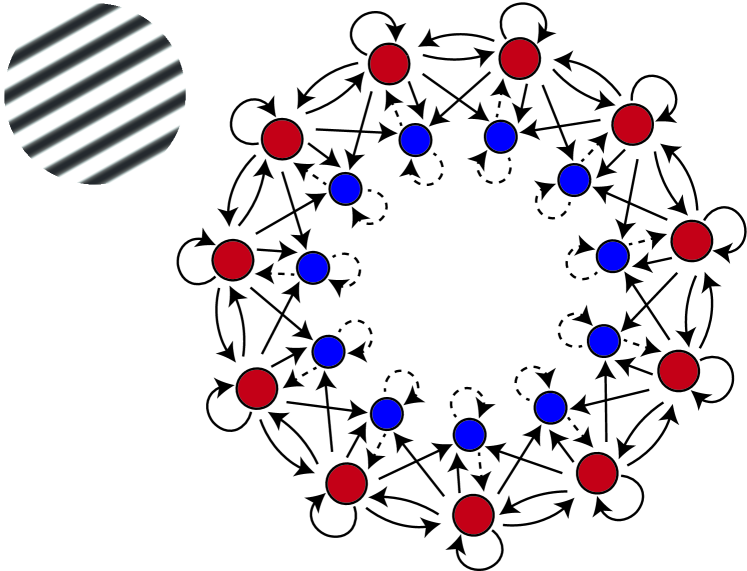
Figure 6: SSN circuit. The circuit consists of 11 excitatory (red) and 11 inhibitory neurons (blue) and receives a sinusoidal grating input shown on the left. The arrows schematize the connections between the different neurons. E-E and I-E connections are excitatory (solid arrows) fully connected, whereas E-I and I-I connections are self-inhibitory (dashed arrows).

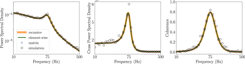
Figure 7: Spectral density (auto and cross) and coherence for the SSN circuit. We plot the power spectral density (left), the absolute cross-power spectral density (middle), and the coherence (right) for a given stimulus each calculated via simulation, the rational function solutions (recursive and element-wise), and the matrix solution (Eq. 3). The PSD is calculated for the excitatory neuron with the highest preference for the stimulus (i.e., exhibiting maximum firing rate). The cross-PSD and coherence are calculated between the two excitatory neurons with the highest firing rates. We use the following parameters for simulating the model: Contrast $c=50$, stimulus length $l=9$, $\Delta x=3.0$, $\sigma_{RF}=0.125\Delta x$. Time constants of $\tau_{\mathrm{E}}=6$ms and $\tau_{\mathrm{I}}=4$ms. Supralinear activation parameters $n=2.2$ and $k=0.01$. See Supplemental Material for the parameters associated with the weight matrices. We add zero-mean Gaussian noise to the SDEs describing the activity of the E and I neurons with standard deviation $\sigma=0.01$.

The Stabilized Supralinear Network (SSN) [22, 23] is a neural circuit model reproducing divisive normalization approximately [24, 25] that has been used to simulate neuronal activity in the sensory cortex [23, 22, 29, 30, 31]. We implement an SSN for simulating the activity of the primary visual cortex (V1) as described in [22]. We consider a 1-dimensional spatial input which is a sinusoidal grating of a fixed orientation and a given contrast (n.b., the response of V1 neurons is tuned to specific positions, orientations, size, etc., of the visual stimulus [32]) and varies with Michelson contrast, $c=(I_{\max}-I_{\min})/(I_{\max}+I_{\min})$, where $I_{\min,\max}$ are the minimum and maximum luminance in the stimulus. The input evaluated at a set of discrete points $\mathbf{x}$, is taken to be proportional to the contrast, $\mathbf{h}(\mathbf{x})\propto c$, and decays with distance from the origin (see Supplemental Material for the precise functional form). We operate in a regime where the circuit exhibits a fixed point solution with damped oscillations (for parameters see Fig. 7 and Supplemental Material).

The dynamical equations for the firing rates of the excitatory neurons, $\mathbf{r}_{\mathrm{E}}(\mathbf{x})$, and the inhibitory neurons, $\mathbf{r}_{\mathrm{I}}(\mathbf{x})$, are given by

$$\begin{split}\tau_{\mathrm{E}}\frac{\mathrm{d}\mathbf{r}_{\mathrm{E}}(\mathbf{x})}{\mathrm{d}t}&=-\mathbf{r}_{\mathrm{E}}(\mathbf{x})+\mathbf{r}_{\mathrm{E}}^{ss}(\mathbf{x})+\sigma\mathbf{\eta}_{\mathrm{E}}(\mathbf{x})\\ \tau_{\mathrm{I}}\frac{\mathrm{d}\mathbf{r}_{\mathrm{I}}(\mathbf{x})}{\mathrm{d}t}&=-\mathbf{r}_{\mathrm{I}}(\mathbf{x})+\mathbf{r}_{\mathrm{I}}^{ss}(\mathbf{x})+\sigma\mathbf{\eta}_{\mathrm{I}}(\mathbf{x})\end{split}$$ (31)

where $\tau_{\mathrm{E}}$ and $\tau_{\mathrm{I}}$ are the time constants of the excitatory and inhibitory neurons, $\sigma\mathbf{\eta}_{\mathrm{E}}(\mathbf{x})$ and $\sigma\mathbf{\eta}_{\mathrm{I}}(\mathbf{x})$ are zero-mean uncorrelated Gaussian noise vectors with standard deviation $\sigma$, and $\mathbf{r}_{\mathrm{E}}^{ss}$ and $\mathbf{r}_{\mathrm{I}}^{ss}$ are the steady-state responses of the excitatory and inhibitory neurons, given by the equations

$$\begin{split}\mathbf{r}_{\mathrm{E}}^{ss}(\mathbf{x})&=k([\mathbf{h}(\mathbf{x})+\mathbf{W}_{\mathrm{EE}}\mathbf{r}_{\mathrm{E}}(\mathbf{x})-\mathbf{W}_{\mathrm{EI}}\mathbf{r}_{\mathrm{I}}(\mathbf{x})]_{+})^{n}\\ \mathbf{r}_{\mathrm{I}}^{ss}(\mathbf{x})&=k([\mathbf{h}(\mathbf{x})+\mathbf{W}_{\mathrm{IE}}\mathbf{r}_{\mathrm{E}}(\mathbf{x})-\mathbf{W}_{\mathrm{II}}\mathbf{r}_{\mathrm{I}}(\mathbf{x})]_{+})^{n}\end{split}$$ (32)

Here, $[z]_{+}=\max(z,0)$ denotes a ReLU activation. In the SSN, the steady-state responses depend on a supralinear activation ($n=2.2$ and $k=0.01$) of the input to the neurons, which is a sum of the stimulus input and feedback from the neurons in the population. The strength of the connections between E-E (excitatory to excitatory) and I-E (inhibitory to excitatory) neurons are encoded in the weight matrices $\mathbf{W}_{\mathrm{EE}}$ and $\mathbf{W}_{\mathrm{IE}}$, which decay like Gaussians as a function of distance from the preferred stimulus. The E-I and I-I connections are not fully-connected but self-inhibitory, with diagonal weight matrices $\mathbf{W}_{\mathrm{EI}}$ and $\mathbf{W}_{\mathrm{II}}$, respectively.

We simulate a 22-dimensional system, see Fig. 6 for an illustration. In Fig. 7, we show the power spectral density for the excitatory neuron with the highest preference for the stimulus (viz., that is maximally firing); the absolute cross-power spectral density and the coherence between the two excitatory neurons with the highest firing rates, each using Welchfls method [28] (simulation), our recursive and element-wise rational function solutions, and the matrix solution (Eq. 3). We confirm that all the solutions match across the entire range of frequencies.

IV.4 Rock-Paper-Scissors

The game of Rock-Paper-Scissors, where rock smashes scissors, scissors cut paper, and paper wraps rock has been employed by evolutionary biologists to investigate the interactions between competing populations of species, where one species has an advantage over only one of its opponents. The game dynamics that describe the evolution of the populations following a particular strategy can be examined with the use of evolutionary game theory [26]. We explore the evolution of this dynamical system in accordance with a sociological model [33, 34], where each population, following a unique strategy, seeks to minimize the difference between the average payoff of the population and the individual payoff.

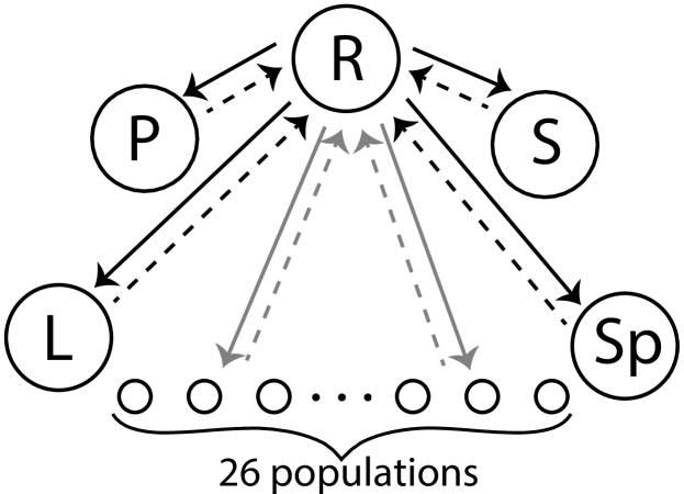
Figure 8: 31-D Rock-Paper-Scissors model. Circles represent the different strategies (31) in the evolutionary game theoretic model. Shown in the figure are 5 of the 31 strategies: Rock (R), paper (P), Scissors (S), Spock (Sp), and Lizard (L). We consider a model with global mutations, i.e., each population associated with a strategy mutates into every other population with the same rate $\mu$. Depicted in the figure are mutations to (dashed arrows) and from (solid arrows) the Rock population.

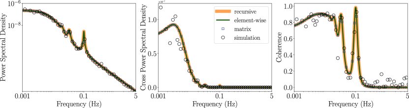
Figure 9: Spectral density (auto and cross) and coherence using different methods for a 31-dimensional Rock-Paper-Scissors type model. We plot the power spectral density (left), the absolute cross-power spectral density (middle), and the coherence (right) for a fixed mutation parameter ($\mu=0.0005$) each calculated via simulation, the rational function solutions, and the matrix solution. The PSD is calculated for the Rock population. The cross-PSD and coherence are calculated between the Rock and Paper populations. We consider the case of multiplicative noise, $\sigma x_{j}$, added to each population, with standard deviation $\sigma=10^{-4}$.

Mathematically, we can represent the system as follows: Let $\mathbf{x}=[x_{1},x_{2},...,x_{n}]$ be the $n$-dimensional system comprising the fractional populations corresponding to different strategies. The sociological model dictates that these fractional populations evolve according to a metric given by $\dot{x_{i}}\propto(f_{x_{i}}-\phi)$, where $f_{x_{i}}$ is the individual payoff for choosing a strategy corresponding to the population $x_{i}$, and $\phi$ is the average payoff of the population given by $\phi=\sum_{i=1}^{n}x_{i}f_{x_{i}}$. It is important to note that the dynamical system is effectively $n-1$ dimensional due to the mass conservation equation $\sum_{i=1}^{n}x_{i}=1$.

We consider a 31-dimensional ($n=31$) version of the Rock-Paper-Scissors game, consisting of 31 populations each following a unique strategy, described by the pay-off matrix, $\mathbf{P}$. See Supplemental Material for a 5-dimensional, Rock-Paper-Scissors-Lizard-Spock version of the game, alongside the analytical solution for its auto-spectrum. For an $n$-dimensional version of the game, the payoff matrix ($P_{ij}$) can be summarized as,

$$P_{ij}=\begin{cases}(-1)^{i+j+1}&i>j\\ 0&i=j\\ (-1)^{i+j}&i<j.\end{cases}$$ (33)

Here, 1 indicates a win against the opponent, $-1$ indicates a loss and 0 indicates neither a win nor a loss (a draw). Therefore, the individual payoff for a given strategy is given in terms of $\mathbf{P}$ as, $f_{x_{i}}=\sum_{j=1}^{n}P_{ij}x_{j}$.

In addition to the populations evolving according to the sociological strategy, we also consider the effects of global mutations and fluctuations in population. For the global mutations, we introduce a parameter $\mu$ such that each population mutates into every other population with constant rate $\mu$, as illustrated in Fig. 8. This results in a stochastic dynamical system where the deterministic part evolves according to replicator-mutator dynamics [35, 26]. Furthermore, we model the noise as multiplicative Gaussian white noise, $\sigma x_{i}\eta_{i}$, with standard deviation $\sigma$ small enough that the population stays close to the fixed point. Thus, for the $n$-dimensional system, we can represent the set of differential equations for all $i\leq n$ as follows:

$$\frac{\mathrm{d}x_{i}}{\mathrm{d}t}=x_{i}(f_{x_{i}}-\phi)+\mu\biggl{(}-(n-1)x_{i}+\sum_{\begin{subarray}{c}j=1\\ j\neq i\end{subarray}}^{n}x_{j}\biggr{)}+\sigma x_{i}\eta_{i}$$ (34)

To ensure that mass conservation is followed, we define the system according to the replicator-mutator differential equation (Eq. 34) for $i\leq n-1$, and compute the $n$-th population from the constraint $\sum_{i=1}^{n}x_{i}=1$. Recall that the individual payoff is $f_{x_{i}}=\sum_{i=1}^{n}P_{ij}x_{j}$, and the average payoff of the population is $\phi=\sum_{i=1}^{n}x_{i}f_{x_{i}}=0$. The dynamical system has a fixed point at $x_{i}^{ss}=1/n$, for all $i\leq n$. Additionally, the elements of the Jacobian, $J_{ij}$, for the dynamical system evaluated at the fixed point can be defined as a function of the mutation rate parameter $\mu$,

$$J_{ij}=\begin{cases}\begin{cases}0&j\text{ is even}\\ (-1)^{i}\times 2/n&j\text{ is odd}\\ \end{cases}&i>j\\ (-1)^{i}/n-\mu n&i=j\\ \begin{cases}(-1)^{i}\times 2/n&j\text{ is even}\\ 0&j\text{ is odd}\\ \end{cases}&i<j.\end{cases}$$ (35)

We simulate a 31D system with a fixed mutation parameter, $\mu=0.0005$, and the scaling factor of the noise, $\sigma=10^{-4}$, that is the same for all the populations. In Fig. 9 (Fig. S4 for the 5-D version), we show the power spectral density for the Rock population (viz., the first strategy), the absolute cross-power spectral density and the coherence between the Rock and Paper populations (viz., the first and second strategy), each using Welchfls method [28] (simulation), our recursive and element-wise rational function solutions, and the matrix solution (Eq. 3). Our solutions match across the entire range of frequencies, verifying their correctness.

V Discussion

In this work, we presented two approaches for computing explicitly the rational function solution of the power spectral density matrix for stochastic linear time-invariant systems driven by Gaussian white noise. In one approach, we derived element-wise solutions (valid for arbitrary $n$-dimensional LTI systems) for the rational function coefficients of any given entry of the PSD matrix, computable in roughly $\mathcal{O}(n^{4}\log n)$ operations. Each coefficient is expressed in terms of Bell polynomials [17] evaluated on submatrices of the Jacobian, defined according to the algorithm summarized in Fig. 2. Our element-wise solution is particularly useful to gain insights into the dependence of the PSD on the model’s functional form and its parameters, especially when the model is fairly low dimensional. Therefore, we provide explicit solutions for the auto-spectra of a general $n=2,3$ and $4$ dimensional system driven by uncorrelated Gaussian noise increments. A similar, albeit longer, symbolic expression can be obtained for any dimensional system and noise correlation structure via our software package (or working through the general solution in Supplemental Material), see section VI. We also showed that the polynomial matrix coefficients in the numerator and the polynomial coefficients in the denominator can be obtained recursively by means of a Faddeev-Leverrier-type algorithm in $\mathcal{O}(n^{4})$ operations. Since the algorithm involves simple matrix multiplication and trace operations, it should be possible to further optimize it to achieve better time complexity. Crucially, both our solutions are free of matrix inverses, in addition to being more revealing than the simpler matrix solution given by Eq. 3.

Finally, we applied our approaches for the derivation of analytical (i.e., closed form) PSD of stochastic nonlinear dynamical models of neural systems, namely Fitzhugh-Nagumo ($n=2$), Hindmarsh-Rose ($n=3$), Wilson-Cowan ($n=4$), and the Stabilized Supralinear Network ($n=22$), as well as of an evolutionary game-theoretic model with mutations ($n=5,31$).

Our solutions should find broad applicability in the analysis of the dynamics of stochastic biological systems exhibiting fixed point solutions, as well as in the broader context of dynamical systems and control theory.

VI Code availability

The code for the general solutions of the auto- and cross-spectrum used to generate the figures can be found at https://github.com/martiniani-lab/spectre.

Appendix A Rational function decomposition of the PSD

The power spectral density of the LTI SDE described in Eq. 2 can alternatively be written as the inverse of the Hermitian positive definite matrix (see Supplemental Material), assuming that $\mathbf{C}\equiv\mathbf{L}\,\mathbf{D}\,\mathbf{L}^{\top}$ is positive definite,

$$\begin{split}\mathbfcal{S}(\omega)=&\bigl{[}\mathbf{J}^{\top}{\mathbf{C}}^{-1}\mathbf{J}+\omega^{2}{\mathbf{C}}^{-1}\\ &+\dot{\iota}\omega(\mathbf{J}^{\top}{\mathbf{C}}^{-1}-{\mathbf{C}}^{-1}\mathbf{J})\bigr{]}^{-1}\end{split}$$ (36)

This enables us to efficiently compute the matrix inverse by Cholesky decomposition. We can recast $\mathbfcal{S}(\omega)$ as a rational function and upon expanding Eq. 3 in terms of the adjugate and determinant matrices, we find,

$$\begin{split}\mathbfcal{S}(\omega)&=(\dot{\iota}\omega\mathbf{I}+\mathbf{J})^{-1}\,\mathbf{C}\,(-\dot{\iota}\omega\mathbf{I}+\mathbf{J})^{-\top}\\ &=\frac{\mathrm{adj}(\mathbf{J}+\dot{\iota}\omega\mathbf{I})\,\mathbf{C}\,\mathrm{adj}^{\top}(\mathbf{J-\dot{\iota}\omega\mathbf{I})}}{\mathrm{det}(\mathbf{J}+\dot{\iota}\omega\mathbf{I})\,\mathrm{det}(\mathbf{J-\dot{\iota}\omega\mathbf{I}})}\\ &=\frac{\mathbf{Z}(\omega)}{Q(\omega)}\end{split}$$ (37)

Here, $\mathbf{Z}(\omega)$ is a complex polynomial matrix representing the numerator of the solution, and $Q(\omega)$ is an even-powered polynomial of degree $2n$ representing the denominator of the solution. When we express the adjugate of the matrices in terms of the corresponding cofactor matrices, it is apparent that $\mathbf{Z}(\omega)$ contains complex polynomials of degree $2n-2$ with even powers of $\omega$ being real and odd powers of $\omega$ being imaginary.