Evaluating Machine Learning Models with NERO:
Non-Equivariance Revealed on Orbits

Abstract

Proper evaluations are crucial for better understanding, troubleshooting, interpreting model behaviors and further improving model performance. While using scalar-based error metrics provides a fast way to overview model performance, they are often too abstract to display certain weak spots and lack information regarding important model properties, such as robustness. This not only hinders machine learning models from being more interpretable and gaining trust, but also can be misleading to both model developers and users. Additionally, conventional evaluation procedures often leave researchers unclear about where and how model fails, which complicates model comparisons and further developments. To address these issues, we propose a novel evaluation workflow, named Non-Equivariance Revealed on Orbits (NERO) Evaluation. The goal of NERO evaluation is to turn focus from traditional scalar-based metrics onto evaluating and visualizing models equivariance, closely capturing model robustness, as well as to allow researchers quickly investigating interesting or unexpected model behaviors. NERO evaluation is consist of a task-agnostic interactive interface and a set of visualizations, called NERO plots, which reveals the equivariance property of the model. Case studies on how NERO evaluation can be applied to multiple research areas, including 2D digit recognition, object detection, particle image velocimetry (PIV), and 3D point cloud classification, demonstrate that NERO evaluation can quickly illustrate different model equivariance, and effectively explain model behaviors through interactive visualizations of the model outputs. In addition, we propose consensus, an alternative to ground truths, to be used in NERO evaluation so that model equivariance can still be evaluated with new, unlabeled datasets.

An ML model has inputs $X$ and outputs $Y$. $G$ is a transformation group acting on $X$ with $\phi$, and on $Y$ with $\tilde{\phi}$. The group element $g\in G$ transforms $x$ to $x^{\prime}=\phi(g,x)$; the set of all possible transforms is the orbit $G(x)$. The model applied to $x$ is $\hat{y}=h(x)$, though this is not used in our method. Rather, the ground truth $y\in Y$ is transformed by $g$ to $\tilde{\phi}(g,y)$, which serves as ground truth to evaluate (here with loss function $l$) the result $h(x^{\prime})$ of evaluating the model on transformed input $x^{\prime}$. The $\mathrm{NERO}_{G,x}$ plot visualizes loss over the orbit $G(x)$.

1 Introduction

Applications of machine learning (ML), and deep learning (DL) more specifically, have enhanced and accelerated many research areas, such as computer vision [26, 31, 83] and natural language processing [24, 8, 19]. Thorough evaluation of ML models may deepen understanding of their functioning, and drive further improvements. The evaluation process in ML, unfortunately, remains largely unchanged over the past decade, which hinders interpretation and innovation.

Model quality is typically measured with a scalar, such as accuracy for classification tasks, precision and recall for object detection, and mean squared error for more quantitative tasks. Though straight-forward, comparing models via scalar metrics can miss important details, limiting insight for ML researchers, and creating ambiguities for practitioners. Two models can be quantitatively similar on average, but respond very differently to meaningfully changing individual inputs. Fig. 1 illustrates two models trained to recognize humans crossing streets.

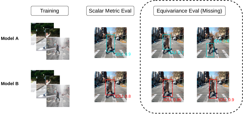
Figure 1: An example of scalar metric being ambiguous and misleading. Suppose object detection model $A$ and $B$ have been trained on the same dataset to detect human that is crossing the street. With standard evaluation procedure, both models are tested with some images and compared via Intersection Over Union (IOU). Model $A$ does a slightly better job than $B$. However, current result fails to characterize models in a more complete way. As shown in the dotted box, model $A$ might perform worse in corner yet important cases where the person is at the edge of the image, in which model $B$ has an advantage.

A model that responds erratically to translating the field of view (which should only translate the predicted bounding box) may be less trustworthy than one that performs better on average on a fixed test set.

Empirical science provides especially challenging areas for applied ML, for at least two reasons. First, specialized instrumentation means data is expensive to gather and labor-intensive to label. Popular ML models, however, need large training datasets, in part due to the simplicity of their scalar metric evaluations. The gold-standard dataset for image object detection, Microsoft COCO [55], has $328,000$ labeled images, and the more recent Object365 [75] has over $2$ million. The ubiquity of ML for object detection justifies and amortizes the cost of creating such datasets, but this scaling does not generally apply to experimental science. Second, scientists in particular value robustness, predictability and understandability in their computational tools [65], in contrast to the black-box nature of deep learning. These issues have catalyzed research in interpretable machine learning (IML) [25], which seeks to intelligibly reveal ingredients of ML model predictions.

Our work complements IML research by revealing how ML models respond to changing inputs, in a way that is intuitive but mathematically grounded. We focus on equivariance, which captures how changes in model inputs map to changes in outputs. In Fig. 1, for example, translating the input image should consistently correspond to translations of the output bounding box. We organize our visualization of model equivariance around a mathematical group of input transformations and the set of all transformations (the orbit) of a given input. This is captured in our proposed Non-Equivariance Revealed on Orbits (NERO) Evaluation, which shows how equivariant a model is, and the structure of its equivariance failures. In settings where practitioners can reason about their analysis task in terms of mathematically predictable responses to data transforms, NERO evaluation gives an informative and detailed picture of ML model performance that is missing from prior scalar summary metrics.

The contributions of this paper, are:

1. NERO Evaluation, an integrated workflow that visualizes model equivariance in an interactive interface to facilitate ML model testing, troubleshooting, evaluation, comparison, and to provide better interpretation of model behaviors,

2. and consensus, a proxy for ground truth that helps evaluate model equivariance with unlabeled data.

2 Related Work

2.1 Equivariant Neural Networks (ENNs)

Improving model equivariance has become a popular ML research topic. Models that are more equivariant have better generalization capability [85], an important goal of applied ML research. Equivariance sometimes occurs naturally in neural networks [64], but guaranteeing equivariance requires more dedicated efforts. Various works focus on improving equivariance of convolutional neural networks (CNN) with respect to rotations [21, 49, 20, 85], shifts [91, 5, 29, 48, 12], and scales [89, 46, 87, 34, 78] through network architectural designs. Data augmentation during training is also effective for improving equivariance [18], with examples in generative models [3, 40, 62, 76], Bayesian methods [80], and reinforcement learning [22, 70].

Existing work often implicitly assumes that more equivariant models will have lower errors when tested on large datasets, due to the close relationship between equivariance and robustness [29, 50]. In fact, equivariance is indeed a close proxy for model robustness, as both represent the model’s ability to perform well on new dataset with or without similar distribution as the training dataset, which is why the works mentioned above apply the same evaluation process using standard scalar metrics for equivariance evaluations. But still, the absence of evaluations directly showing model equivariance hinders more accurate understanding of model behaviors, which inspired our work on NERO evaluation.

2.2 Interpretable Machine Learning (IML)

Deep neural networks (DNN) have achieved great success in a variety of applications involving images, videos, and audio [51]. However, advances in DNN research are generally more empirical than theoretical [67]. DNN models thus still largely work as black boxes, limiting how practitioners interpret and understand model predictions [6, 25].

IML research addresses this with methods based on various different strategies that can be broadly summarized as: model components, model sensitivity, and surrogate models [56, 39, 82, 63]. Of the three, surrogate models [37, 73, 72] are not described further here since they have little methodological connection to NERO evaluation. Visualizations for IML seek to transform abstract data relationships into meaningful visual representations [42]. Studies have shown that interactive visualization is a key aspect of sense-making when it comes to combining visual analytics with ML systems, which shapes our designs in presenting NERO evaluation through an interactive interface [14].

Model Components. IML work focusing on model components visualize the internals of a neural network. Abadi et al. [1] developed dataflow graphs in TensorFlow [1], which visualizes the types of computations that happen within a model, and how data flows through these computations. Following this work, Smilkov et al. [77] improved the dataflow graph by showing weights sent between neurons using different colors, curves, line thickness, as well as feature heatmaps. Plots in our NERO evaluation interface do not similarly visualize model components, but do employ similar visualization ingredients.

Beyond static visualizations, Yosinski et al. [90] designed interactive visualizations of learned convolutional filters in neural networks, and Kahng et al. [45] designed interactive system ActiVis for visualizing neural network responses to a subset of instances. The ActiVis interface supports viewing neuron activations at both subset and instance level, similar to our NERO interface, though the underlying quantities visualized and the goals differ.

Feature Importance. Instead of visualizing model components, other approaches show feature importance by analyzing how model predictions change in response to changes in input data, in a way that is agnostic to the ML model choice. Friedman’s Partial Dependent Plot (PDP) [33] reveals the relationship between model predictions and one or two features by plotting the average change in model prediction when varying the feature value. Goldstein et al. [36] built on this with Individual Conditional Expectation (ICE) plots that show model prediction changes due to changing features in individual data points, rather than the average.

Subsequent works visualize expected conditional feature importance [11], conduct sensitivity analysis [79], and improve PDP with less computation cost [4]. Lundberg et al. [57] present SHapley Additive exPlanations (SHAP) that assigns each feature an importance value to explain why a certain prediction is made. Zhang et.al. [92] derived a more robust, model-agnostic method from high-dimensional representations to measure global feature importance, which facilitates interpreting internal mechanisms of ML models. While NERO evaluation also employs data transformation and a response-recording mechanism, and is also model-agnostic, it does not visualize feature importance per se. Instead, it collects model responses with respect to data transformed by group actions as a whole, and supports visualizations at both aggregate (group) and instance levels.

3 Mathematical Background

3.1 Group Action and Group Orbit

We give a concise summary of some elements of group theory, a rich topic meriting deeper consideration [74]. A group $G$ is a set with an operation “$\cdot$”$:G\times G\rightarrow G$ that is associative ($(f\cdot g)\cdot h=f\cdot(g\cdot h)$), with an identity element $e$ ($g\cdot e=e\cdot g=e$), and with inverses ($g\cdot g^{-1}=g^{-1}\cdot g=e$). A group action of group $G$ on set $X$ is a function $\phi:G\times X\rightarrow X$ that transforms an $x\in X$ by $g,h\in G$ according to $\phi(g,\phi(h,x))=\phi(g\cdot h,x)$ and $\phi(e,x)=x$. The orbit of $x\in X$ under a group action $\phi$ is the set of all possible transformations $G(x)=\{\phi(g,x)|g\in G\}$. We use group orbits to generate a mathematically coherent family of ML model inputs, with which (human) users of the model can predict and reason about corresponding model outputs. For example, Fig. 2 illustrates a single $28\times 28$ MNIST [52] digit image $x$, and its orbit under the rotation group $SO(2)$ through the space $X$ of all possible $28\times 28$ images.

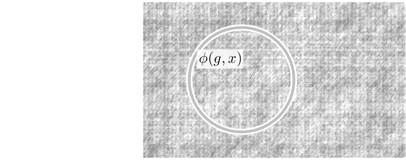
Figure 2: The group $G$ of 2-D rotations, left, acts on the set $X$ of images, right. An $x\in X$, a “4” digit, is rotated to $\phi(g,x)$ for a $g\in G$ via group action $\phi$, part of the orbit $G(x)\subset X$ of all rotations of $x$.

We currently make NERO plots for spatial transformation group actions (shifts, rotations, flips), which have natural spatial layouts (e.g. the circular domain of $SO(2)$), but we want to highlight that NERO plots should in principle work with any group that has an intelligible layout.

3.2 Equivariance

Three terms – invariance, equivariance, covariance – for describing the relationship between changes in inputs and outputs of ML models [60], can be introduced via a commutative diagram (1).

(1)

The ML model hypothesis $h$ maps from inputs $X$ to outputs $Y$. For some group element $g$, actions $\phi(g)$ and $\tilde{\phi}(g)$ transform $X$ and $Y$, respectively. Assuming (1) is true for some model (i.e., hypothesis $h$ and transform $\tilde{\phi}(g)$ always reach the same output as input transform $\phi(g)$ followed by $h$), the following definitions describe how.

The model is invariant with respect to the group action $\phi$ if $\tilde{\phi}=I$, the identity transform on $Y$. In classification tasks, invariance means that the classification result is unchanging while inputs are transformed in some way. A model is equivariant when the model inputs and outputs are transformed in the same way: $\phi=\tilde{\phi}$. For example, in object detection, where model outputs are object bounding boxes, if the object is shifted 5 pixels to the right, an equivariant model would predict the bounding box 5 pixels to the right. Covariance is an extension of equivariance in which $\phi$ and $\tilde{\phi}$ are mathematically distinct (because $X$ and $Y$ have distinct types), but have a semantic linkage necessitated by the structure of group $G$. For example, in optical flow recovery from image sequences, rotating the image inputs to a covariant model will produce an output in which both the vector field domain and the vectors themselves are correspondingly rotated. By a slight abuse of terminology, we use “equivariance” in this work to refer to all three commutative diagram properties.

4 Method

4.1 Overview

Diagram (1) describes an ideal, perfectly equivariant model. Real models, applied to real data, often fall short of this; NERO evaluations seek to reveal how through visualizations. Fig. Evaluating Machine Learning Models with NERO: Non-Equivariance Revealed on Orbits defines the NERO plot as inspired by diagram (1): the thickest arrows at the center of the figure, within and between $X$ and $Y$, roughly correspond to the arrows of (1). Input $x$, however, maps to ground truth $y$ rather than model output $h(x)$, and the purpose of the NERO plot is to visualize the gap between $h(x^{\prime})$ and $y^{\prime}$, where $h(x^{\prime})$ is the model output on transformed input $x^{\prime}$, and $y^{\prime}=\tilde{\phi}(g,y)$ is the transformed ground truth $y$. This illustration uses an abstract depiction of group $G$ to schematically indicate $G(x)$ and $G(y)$, but some particular spatial layout of $G$ necessarily determines the shape of the NERO plot. If the model is equivariant, then $h(x^{\prime})=y^{\prime}$, so the NERO plot is a flat constant. The visual structure of a non-constant NERO plot shows the structure of model non-equivariance over the group orbit domain.

The quantity shown in a NERO plot is some scalar metric (understandable to practitioners) that measures the gap between $h(x^{\prime})$ and $y^{\prime}$, including the standard metrics of model prediction confidence, accuracy, mean square error (MSE) and more generally speaking, error metrics. The NERO plot illustrated in Fig. Evaluating Machine Learning Models with NERO: Non-Equivariance Revealed on Orbits (right) is an individual NERO plot, as it depicts model non-equivariance along the group orbit $G(x)$ around an individual input sample $x$.

While §1 critiqued single scalars to summarize model results over a large dataset, informative NERO plots can also involve averaging. An aggregate NERO plot visualizes the average scalar metric over a dataset, or subset of it, at each point along the group orbit (i.e. with the same domain as the individual NERO plot), to show trends in the model’s response to transformed inputs. Like PDP and ICE plots (§2.2), NERO plots evaluate the model within some neighborhood around a given sample, but instead of varying features in isolation, we traverse the orbit of some interpretable transform group.

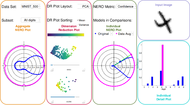
Figure 3: The NERO interface has $5$ sections: aggregate NERO plot, dimension reduction (DR) plot, individual NERO plot, input image, and detail plot. Each section is highlighted with orange, red, dark green, purple or cyan bound box respectively, where bounding boxes are not part of the interface design. The sections are interactively controlled, with linked views.

To try to see degrees of freedom lost in the aggregate NERO plot, we can also treat the individual NERO plots as $n$-vectors, and use dimensionality reduction. The resulting dimension reduction (DR) scatterplot organizes data points according to the similarity of their patterns of non-equivariance, to help localize abnormal model behavior and identify the connections between worse-performing cases.

All of these visualizations are linked together in the interactive NERO interface that provides users with both the convenience to see model equivariance in a high-level view across a whole dataset (through the aggregate NERO plot), as well as navigating into detail views (through the individual NERO plot, e.g., a specific place in the orbit where the model has trouble).

The following subsections describe the components of NERO evaluation through a digit recognition task with MNIST dataset [52], with the group action of continuous rotation around the image center.. NERO evaluation is presented via an interactive NERO interface, an example of which is in Fig. 3, starting with the individual NERO plot on the right, The goal of using this task and MNIST dataset, is to utilize a well-known, easy-to-interpret task as an example to make the illustrations of NERO evaluation more concretely, instead of limiting or bounding NERO evaluation to only such or similar tasks, as we will be showcasing how it could be applied to different use cases in §5. The CNN model here has six cascaded convolutional layers, six batch normalization (BN) layers [44], six rectified linear units (ReLU) [35], followed by two fully connected layers. The detailed network architecture is illustrated in Fig. 4, but we would like to point out that NERO evaluation is model-agnostic, and the purpose of explaining model structure is to ensure reproducibility.

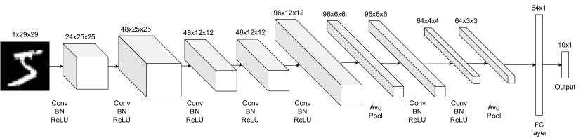
Figure 4: Network structure of the CNN model for digit recognition with MNIST [52]

For the proposed NERO evaluation to be effective, the first criteria is to ensure that the associated NERO plots are distinguishable enough when evaluated on two models with different equivariance. To illustrate how NERO plots differ on equivariant and non-equivariant models, the network in Fig. 4 is trained twice, first without and then with rotational data augmentation, to create two models that predictably differ. The augmentation model should have better invariance, even though the total amount of training (with or without augmentation) is the same.

4.2 Individual NERO Plot

Individual NERO plots (Fig. 3 right) visualize model equivariance for a single sample. The NERO metric in this case is confidence: the probability of correct classification. Individual NERO plot displays polar plots of confidence over the image rotation angle $\theta$, for a particular input image of a “4” (Fig. 3 upper-right corner). For a model with perfect rotational equivariance, the individual NERO plot will be a circle, while any dips indicate non-equivariance. The NERO plots for the original model trained without data augmentation, and for the DA model trained with augmentation, are in blue and magenta, respectively.

The plots confirm our expectation that the DA model is more equivariant, with the magenta plot being a near-perfect circle, while the blue (original model) plot is highest at small rotation angles, which proves the plot being distinguishable between different models. For a single interactively selected rotation angle (green line in polar plot), the details of the models’ predictions are shown as a bar chart (Fig. 3 lower-right corner) showing confidences for all possible digits. Such a detail view is necessarily specific to the model task and data type, but the NERO interface should have any visualization of individual plots, input data sample, and model details to be adjacent. Here, the DA model (magenta) has higher confidence in recognizing “4” and essentially zero confidence for any other digit, unlike the original model (blue), which is highest for “4” but with non-zero confidence for other digits.

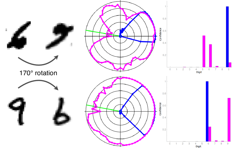
Figure 5: The individual NERO and detail plots of original (blue) and data augmented (magenta) models, for two digits rotated $170^{\circ}$, “6” (top) and “9” (bottom), reveal the extent to which data augmentation overcome the confusion between these two rotated digits.

Some insights about the structure of data and task can be gleaned from individual NERO plots, for example, the digits $6$ and $9$ in Fig. 5. For both digits, the original and DA models perform similarly at zero or small rotations angles while the original model fails as the angle increases (rightward lobe in blue plots), whereas the DA model performs better (though not uniformly) over all angles (magenta plots). The individual NERO plots show that the original model confidence falls to near zero for large angles, but the detail bar charts (Fig. 5 right) provide additional insight: the original model mis-classifies the $170^{\circ}$-rotated $6$ as $9$, and the rotated $9$ as $6$, consistent with these digits’ basic shapes. The DA model does not have the same near perfect equivariance as with the “4” digit of Fig. 3, but the level of equivariance here is still surprising: the DA model (magenta) gives moderate confidence of “6” for the rotated $6$, and highest confidence of “9” for the rotated $9$, with lower confidence for the incorrect digits. The performance of the DA model implies that the shapes of $6$s and $9$s within MNIST are distinct enough (9s having a straighter side) that they may be correctly recognized even with rotation. This exemplifies how individual NERO plots with detail views can not only visualize model equivariance on a single sample, but also help interpret model characteristics. We will show in §5 how individual NERO plots and detail views help visualize equivariance and provide interpretations for other models and tasks.

4.3 Aggregate NERO Plot

Aggregate NERO plots reveal over-all equivariance for a subset of a dataset, or an entire dataset, using the same spatial orbit layout and the same visual encoding as in the individual plots, though the scalar quantity visualized may be different. The aggregate NERO plots on the left side of Fig. 3 show equivariance for $500$ MNIST images, with $50$ images of each digit, using the same polar plots over the circular domain of the rotation group orbit. The aggregate plots, however, show accuracy – the fraction of correct classifications over the input samples – rather than the confidence shown in the individual plots. In our MNIST example, the data augmented model (magenta) is much more equivariant for this subset of images than the original model (blue).

Figure 6: Aggregate NERO plots for the original (blue) model reflect the average rotational symmetry of each digit.

Aggregate NERO plots also reveal additional properties of the task and data. Fig. 6 shows aggregate plots for $50$ images of each digit. Digit $0$ is already rotational invariant, so both original and DA NERO plots show equivariance. The original model (blue) aggregate NERO plot for “1” shows its $180^{\circ}$ rotational symmetry with lobes at $0$ and $180$ degrees; the same holds for $8$ and to a lesser extent for $5$. The lack of rotational symmetry of digits $2$, $3$, $4$, and $7$ are all confirmed by their blue plots. Even though NERO plots cannot answer questions about why a model made the predictions it did (as pursued in other interpretable machine learning work, §2.2), these examples suggest how aggregate NERO plots can be used to help understand patterns of model behavior with specific input classes over specific transforms.

4.4 Dimension Reduction (DR) Plot

Dimension reduction (DR) plots conceptually bridge the information in the aggregate and individual NERO plots, and are thus shown in between them in the NERO interface (second part of Fig. 3). The data vector underlying the individual NERO plot (all the metric values evaluated over the group orbit) is considered as a point in some high-dimensional space, and a dimensionality reduction method is applied to lay out the data points in a 2D scatterplot. Our current interface supports layout via principle component analysis (PCA), independent component analysis (ICA), as well as non-linear ISOMap, t-SNE [81], and UMAP [61]; Fig. 3 shows results with PCA. The intent is that data samples with similar patterns of non-equivariance should be nearby in the DR plot, to give an over-all sense of the varieties of non-equivariance from that model, and to highlight any outlier inputs requiring detailed attention. The scatterplot dots are color-encoded by either the mean or the variance of the individual NERO plot values; mean for showing trends in over-all model performance, and variance for showing which inputs exhibited the best or worst equivariance.

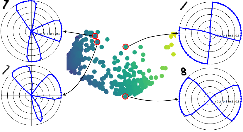
Figure 7: DR plot colormapped by mean confidence, annotated with some associated individual NERO plots.

In our interactive interface, users can click on a dot of interest in the scatterplot to trigger display (to the right) of the corresponding individual NERO and detail plots; in Fig. 3 the selected point is indicated with a small red circle. Fig. 7 shows an expanded view of this scatterplot, annotated with individual NERO plots for selected points. These suggest that the DR plot is successful in presenting a navigable view of the different patterns of non-equivariance, with similar individual plots (Fig. 7 left) arising from nearby points. More distant points have distinct individual plots (Fig. 7 right), though in this case the similarly shaped plots are quantitatively distant because of their different orientations.

4.5 NERO Interface

The previously described components of the NERO interface (Fig. 3) are designed with the general logic of overview on the left and details on the right; this spatial layout is the same across different applications, as will be shown in more case studies in §5. All sections are individually controllable and interactively linked. On the left, the dataset and subset of interest are selected via drop-down menus, with the resulting aggregate NERO plot below. The DR plot section supports choosing the scatterplot layout and coloring, and selection of individual data points within the scatterplot updates individual and detail views to the right. The individual NERO plot domain is the group orbit, and the interface permits moving within the orbit to look at a particular transform of a single sample, with real-time updates of the model output. In the MNIST interface, for example, clicking and dragging within the polar plot selects and changes the rotation angle, and updates the resulting rotated digit image and the models’ outputs from it. Our interface is implemented in PySide (Python bindings for QT) as a desktop application, running on the same machine as the model.

4.6 Consensus

Although existing scalar metrics (accuracy, confidence) serve well as NERO metrics to incorporate easier adaptions for practitioners, NERO evaluation should ideally also work on unlabeled data lacking ground truth. Because, as shown in Fig. Evaluating Machine Learning Models with NERO: Non-Equivariance Revealed on Orbits, equivariance is revealed through the gap between $h(x^{\prime})$ and $y^{\prime}$, which technically should not depend on the existence of ground truth. However, given that existing metrics all require ground truth, an additional modest contribution of this work is consensus, which serves as a proxy for ground truth in the metric evaluation, when making NERO evaluations for models with desired equivariance or covariance (as opposed to invariance). The consensus for input $x$ is roughly the average of the un-transformed model outputs on all transformed inputs within the orbit. Relative to Fig. Evaluating Machine Learning Models with NERO: Non-Equivariance Revealed on Orbits, we have

$$\mathrm{consensus}(x)=\left\langle\tilde{\phi}(g^{-1},h(\phi(g,x)))\right\rangle_{g\in G}$$ (2)

The average $\langle\cdot\rangle_{G}$ depends on the structure of output space $Y$, while $G$ depends on the equivariance of interest. For object detections, $Y$ is the set of bounding boxes defined by corners $(\mathrm{x}_{\mathrm{min}},\mathrm{y}_{\mathrm{min}})$ and $(\mathrm{x}_{\mathrm{max}},\mathrm{y}_{\mathrm{max}})$, and an element $(t_{\mathrm{x}},t_{\mathrm{y}})$ of translation group $G$ acts on the bounding box by component-wise addition. In this case, (2) can be computed by simple arithmetic mean of the translated bounding box corners.

5 Experiments - Applying NERO to More ML Cases

We illustrated in §4 the designs and components of NERO evaluation through a 2D digit classification task with MNIST [52]. As mentioned before, NERO evaluation is model- and task-agnostic. In this section, we demonstrate how NERO evaluation could be applied to different ML models in three different research areas: object detection (classification and localization in 2D photographic images), particle image velocimetry (velocity measurements in fluid dynamics), and point clouds recognition (classification in 3D computer vision) in §5.1, §5.2 and §5.3, respectively. In all subsections, we end with qualitative feedback from PhD students from our institution who are knowledgeable in each area, but not involved in the developmet of NERO evaluation.

5.1 Object Detection

Object detection is a staple of computer vision research, witnessing dramatic advances from deep learning [94, 23]. Despite the great successes, recent research discovers that object detectors can be very vunerable to small translations [59]. And ongoing efforts have been dedicated on developing shift-equivariant neural networks [13, 59]. Unfortunately, evaluations for shift equivariance advancements are still based on the average of scalar metrics such as precision, recall, intersection over union (IOU), or mean average precision (mAP), over the dataset. As noted in §1, however, such summary evaluations give no direct insight about equivariance, which is a natural concern for applications like autonomous driving requiring high equivariance not just by average, but also in corner cases. A person should be recognized as such regardless of their position with the image, which implies an equivariance evaluation over the group of image translations.

For this section, we use the popular Faster R-CNN [71] framework, with the MSCOCO [55] dataset, though the creation and display of NERO plots for this task is independent of model or dataset.

Data Preparation. The architecture of Faster R-CNN does not guarantee translational equivariance, so models with different equivariance properties can be obtained by training with datasets with different augmentations, as we show here. We selected $5$ out of the $80$ MSCOCO classes for demonstration: car, bottle, cup, chair and book. We selected objects that belong to these $5$ classes as key objects and cropped the original images to a $128\times 128$ window around these objects. As shown in Fig. 8, translational shifts (by between $-64$ and $64$ pixels in both directions) are achieved by cropping with shifted bounds, so that the key object positions change within the field of view.

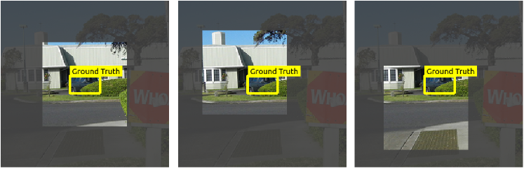
Figure 8: Key objects are shifted by cropping the original MSCOCO image to shifted bounds (the non-masked square).

To ensure interesting cropped images, the MSCOCO images are filtered with following criteria: (1) include a key object whose ground truth class label is in the $5$ selected classes; (2) ensure that for all shifts the cropped fields of view does not extend past the original image edges; and (3) ensure that the key object’s ground truth bounding box is not less than $1\%$ or more than $50\%$ of the cropped $128\times 128$ region.

Model Preparation. We predict that different levels of model equivariance can be created by different levels of random shifts, or jittering, in the training dataset of cropped images. At $0\%$-jittering, key objects are never shifted and stay at the center of the cropped images for training, while at $100\%$-jittering key objects are shifted randomly (uniformly) within the $[-64,64]$ range during training. Jitterings are performed like other data augmentations, i.e., cropping happens at real-time in data loaders. A model trained with $0\%$ jittering is expected to only do well on unshifted images, while a model from $100\%$ jittering is expected to be more equivariant (perform well regardless of shift).

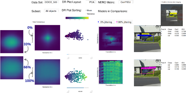
Figure 9: NERO interface for object detection, for models trained with $0\%$ (upper row) and $100\%$ (lower row) jittering. Sections for aggregate, dimension reduction, individual, and detail plots are organized as in the MNIST interface (Fig. 3). Two aggregate NERO plots on left edge show intermediate jittering levels for comparison.

Results. Fig. 9 shows the full NERO interface for models with $0\%$ and $100\%$ jittering. As in the MNIST example of Fig. 3, equivariance of the two models is evaluated and visualized with both aggregate and individual NERO plots, connected with dimension reduction plots, with a different task-appropriate detail display on the right. The left edge of Fig. 9 also shows aggregate NERO plots from two other intermediate jittering levels. Matching our expectations, the amount of jittering is visually reflected in the width of the NERO plot peak, with high equivariance in $100\%$ jittering (lower row) evident in the wide uniform plateau of high values in that heatmap, versus the small bright spot at $0\%$ jittering (upper row) indicating non-equivariance.

Aggregate NERO plots give a quick overview of model equivariance, but individual NERO plots enable detailed investigation. For example, in Fig. 9, the individual NERO for the $100\%$ jittering model has dark regions on the left edge, indicating worse performance at certain shifts. A curious practitioner can simply click on those spots to scrutinize model details, as shown in Fig. 10, which investigates a small change in shift between the top and bottom row.

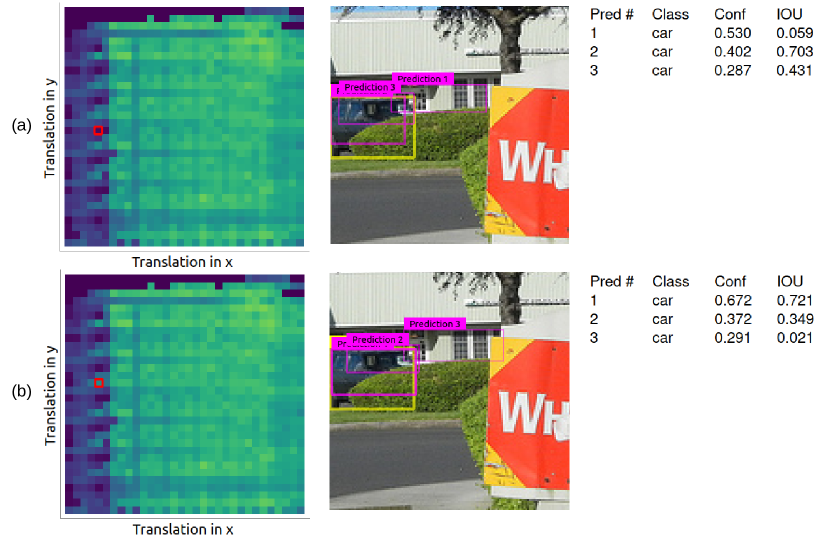
Figure 10: Individual NERO and detail plots further investigating model performance. (a): investigating $100\%$ jittering model’s dark spot on its individual NERO plot. (b): investigating a nearby spot (input image similarly shifted) that has much better results of from the same $100\%$ jittering model.

We learn that at both shifts, the model gives three bounding box predictions, one with a high IOU of about $0.7$, but the confidence ranking of the three boxes is different in the two locations. The individual NERO plot shows the IOU only for the most-confident prediction, creating the dark regions. In this way, NERO plots allow practitioner to explore and understand model edge cases.

Consensus. Consensus (§4.6) in this case is the average of unshifted bounding box predictions from shifted input images. Fig. 11 shows the individual NERO plots computed from ground truth and consensus.

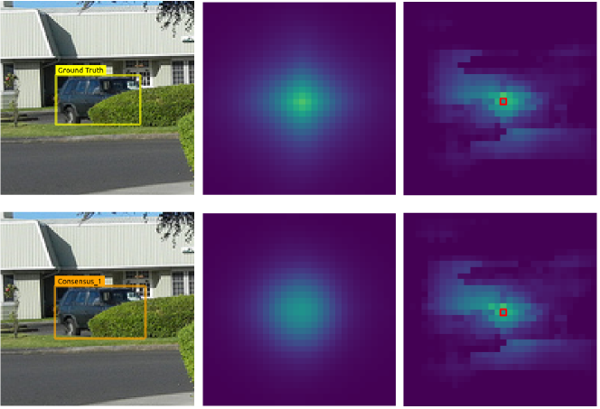
Figure 11: Consensus boxes computed from model outputs (left column), individual NERO plots of each model computed from ground truth (middle column) and from consensus (right column). Subtle differences are highlighted in yellow circles.

The strong similarity of the two plots suggest that, at least for this image, the amount and structure of equivariance shown by NERO plots is nearly the same with or without ground truth, which increases the applicability of NERO plots for unlabeled data.

Expert Evaluation. A researcher in causality for ML, with basic knowledge of equivariance, tried our NERO interface for object detection. The evaluation was semi-guided, meaning that the expert was free to explore himself after we walked him through examples similar to those earlier in this section. The ensuing discussion focused on the NERO plot idea itself and its value; quotes below from the expert are in italics.

It makes sense to compute equivariance like this, it is neat to model it with simple group theories – the expert understood how we transform samples along group orbits, and measure results on transformed samples. Aggregate NERO plots are quick to look at when comparing two models, it’s pretty much as fast as looking at two numbers. – the expert felt that NERO plots do not create excessive visual complexity for users. I am surprised by how different the models can fail equivariance, and the fact that you can just click on these dots to further explore is amazing … – the expert said about the DR plots – … but now I see what are the differences – the expert looking at the corresponding individual and detail plots. Finally, after using the interface for about $10$ minutes, the expert concluded: Using equivariance as an evaluation strategy is interesting and new, I’ve never thought about it, and I am curious to see it with more examples. I think it is quite surprising to see these results, I knew there is more going on underneath the average errors we see everyday, but being able to actually see them and look further inside is amazing. I think it would benefit anyone who cares about model equivariance or develops better ENN’s.

5.2 Particle Image Velocimetry (PIV)

Particle Image Velocimetry (PIV) is an important tool for physicists studying experimentally constructed (as opposed to simulated) fluid dynamics. PIV estimates velocity flow fields from frames of video of illuminated particles moving through a flow domain. Traditional PIV algorithms [86, 41] work for simple flows, but researchers are interested in the promise of ML-based methods for faster computation and complex flows [69, 53, 10, 9].

Empirical scientists expect measurement tools to respect physical symmetries. For example, the world-space flow pattern recovered in PIV should be the same regardless of the coordinate frame of measurement. This corresponds to various rotations and reflections of the image data and covariant changes in the recovered vector fields. Continuous rotations are applicable here (as demonstrated on MNIST §4), but to demonstrate a different kind of NERO plot we worked with the dihedral group $D_{4}$ of symmetries of the square (with reflections and $90^{\circ}$ rotations) [74], times the binary group $\mathbb{Z}_{2}$ for flow reversal, giving a discrete group of $16$ elements. We investigate NERO plots for a PIV ML model to illustrate how evaluating model equivariance may increase trust in novel scientific ML applications, by giving detailed information not captured in existing summary ML evaluations (e.g. RMSE). As PIV is closely related to the computer vision problem of recovering optical flow from video, this example also suggests how NERO plots may work for optical flow models [43].

We compare a traditional (non-ML) Gunnar-Farneback method [30], implemented in OpenCV [7], with a recent deep learning method, PIV-LiteFlowNet-en [9]. Training and test images are obtained from the Johns Hopkins Turbulence Database [54, 66].

Data Preparation. In total, $8,794$ pairs of images covering $6$ different types of flows, namely Uniform, Backstep, Cylinder, SQG, DNS, and Isotropic, are used during training. $120$ image pairs are used in testing when generating the NERO plots.

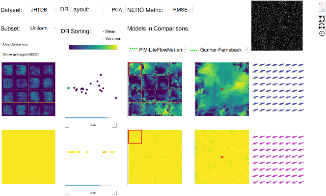
Figure 12: The NERO interface for PIV comparing an ML method (top row) with a non-ML method (bottom row). This has the same sections as in previous interface examples, but with a small-multiples display of the vector field domain for each element of the discrete orbit.

Model Preparation. PIV-LiteFlowNet-en [9] is trained with $8,794$ pairs of particle images as explained above; Gunnar-Farneback does not require training. Both are tested with the same test dataset consisting of $120$ image pairs. Apart from performance as measured by RMSE, we expect Gunnar-Farneback to be naturally equivariant, without bias towards any flow direction. On the other hand, we expect less equivariance from PIV-LiteFlowNet-en, even though the training and testing flow types are the same.

Results. Fig. 12 shows our NERO interface for comparing PIV-LiteFlowNet-en (top row) and Gunnar-Farneback (bottom row). The top right corner shows a controllable animation of the particle image sequence that PIV analyzes. As before, higher equivariance is shown with brighter and more uniform NERO heatmaps; dark spots indicate non-equivariance. Despite the similar use of a heatmap, NERO plots for PIV are richer than those used for object detection (Figs. 9, 10). In object detection NERO plots, each pixel represents one point in the orbit, i.e., a specific shift. Carrying the same idea to PIV would create NERO plots like Fig. 13(a), with $16$ squares for each element of the (discrete) group orbit, as indicated with symbols in each bottom right corner (F is original, F’ is time-reversed, at all possible orientations), with the heatmap showing RMSE over the whole flow domain.

(a)

(b)

Figure 13: NERO plots for PIV with (a) spatially averaged error and (b) detailed display of the per-location error.

Drilling down further, Figs. 13(b) and 12 use a small-multiple display to show $16$ copies of the flow domain, to reveal the spatial locations of flow for which the model was least equivariant. The Show averaged NERO checkbox in the interface toggles between the two.

As expected, Fig. 12 shows that Gunnar-Farneback performs consistently better, with almost perfect equivariance. To investigate further into model outputs, the individual detail plots include an enlarged view of the non-averaged "pixel" in the individual NERO plot, and a vector glyph visualization overlays the predicted field on the ground truth.

Expert Evaluations. A physics researcher with expertise in PIV tried our NERO PIV interface and gave qualitative feedback, in the same format as the previous object detection evaluation. We walked our expert through the basic digit recognition task before letting him use the PIV interface himself. Quotes below from the expert are in italics.

It is very good to be able to see so much more information than an average value, which tells too little of the story. You know, for a turbulence flow the interesting and hard part is not everywhere, often much less than the boring part, so the average error really does not help much. – the expert likes instantly that NERO plots show much richer information than conventional scalar metrics. I like that I am able to locate high-variance (less-equivariant) samples from the dimension reduction plot, you see, this cluster has higher variance, and contains the interesting samples – the expert said when looking at the DR plots – it is really convenient to select individual samples from the DR plots, it really brings out the interesting samples to investigate – the expert thinks the design is effective in helping user traverse through samples and locate the interesting one quickly. Yes, definitely, it [NERO] would save me so much time analyzing PIV model outputs. I’ve been using Jupyter notebook to visualize some parts of the flow but this [NERO] is totally a game changer – the expert said when asked about if he would personally use the interface in his research.

5.3 3D Point Cloud Classification

Point cloud classification is a fundamental task in 3D computer vision that involves assigning semantic labels to 3D point clouds [38]. It has many important applications, including object recognitions [15], scene understanding [17], and robotics [27, 84]. Among many research areas in point cloud classification and analysis, equivariant point cloud classification is a recent development that aims to battle the significant performance downgrade caused by rotations by taking advantage of symmetry and invariance properties of 3D objects [16, 58, 32]. Current procedure on evaluating equivariance of these models is by augmenting random rotations to test datasets and comparing average accuracies, as used in [16] and [58]. As discussed in §2.1, such evaluation process has its drawback that models excelling in the majority of transforms (rotations) will be good enough to excel in average metrics, without real weakspots getting revealed, which hinders interpretability, trust and future developments. In this section, we demonstrate how NERO evaluation mitigates this issue to support this rising research area.

To visualize results from 3D rotations in 2D NERO plots, we conduct our NERO evaluation based on a subset of rotations. More specifically, suppose each rotation is represented via an axis-angle representation, we define each rotation axis to be a 3D vector sitting within one of the three 2D slicing planes, namely x-y, x-z, and y-z plane, with the vector’s one end at the origin. The angle in the axis-angle representation is simply a rotation angle between $0$ and $180$ degrees. The angles between the rotation axis and its horizontal axis in the plane, alone with the value of rotation angle, are visualized intuitively in a polar-coordinate plot, as shown in both aggregate and individual NERO plots in Fig. 14.

For this section, we demonstrate NERO evaluations on the Point Transformer [93] models with ModelNet40 [88] dataset.

Data Preparation. We use the widely adopted ModelNet40 and its subset ModelNet10 dataset [88]. The ModelNet40 dataset contains $12,311$ CAD models with $40$ categories. The dataset is split into $9,843$ training and $2,468$ testing samples. ModelNet10 is a subset of ModelNet40 and only contains $10$ categories, with a total number of $3,991$ training and $908$ testing samples. As a common practice in point cloud classification, we follow the data preparation procedure from Qi et. al. [68] to uniformly sample point clouds from the CAD models.

Model Preparation. When applying deep learning models on point cloud classifications, permutations of the point clouds orderings is another common source of invariance besides rotations. To make this demonstration more predictable, we exclude the effect from permutations by choosing the Point Transformer [93] model, which is by design invariant to permutations thanks to its self-attention operator. To show how NERO evaluations distinguish between a non- and equivaraint model, similar to §4, the Point Transformer model was trained twice, first without and then with rotation augmentation, to create two models that differ predictably. The augmentation model should have better invariance, even though the total amount of training being the same.

Results. Fig. 14 shows the NERO interface for the two models discussed above.

Figure 14: The NERO interface for 3D point cloud classification comparing Point Transformer model trained without (top row) and with (bottom row) rotation augmentations. This has the same sections as in previous interface examples.

As in the MNIST example of Fig. 3, invariances of the two models are evaluated and visualized via aggregate and individual NERO plots, connected with dimension reduction plots, with a different task-appropriate detail display on the right. Looking at the aggregate plots on the left, we can observe that, matching our expectations, the original model (top) has a bright spot at the center, indicating that it only performs well up to small rotations (both axis and rotation angles), whilst the data-augmented model (bottom) has a more uniform display across the plot, indicating that it is much more invariant to rotations.

Individual NERO plots enable detailed investigations. The specific sample shown in Fig. 14 is a bathtub. And its default orientation in the dataset is vertical in terms of the $x$-$y$ plane. From the bright yellow stripe in the top individual plot, we can observe that the original model is only able to recover after rotations along vertical ($z$) axis, which are much easier, while the augmented model (bottom) recognizes the bathtub across all axis-angle represented rotations very well.

Expert Evaluations. We invited the same expert from §5.1 to give us evaluations again. This time, we focused more on collecting expert’s feedbacks about how it feels going from one interface to another.

It feels very similar from the object dection interface to this, the layouts are the same, which is good, I am still able to quickly navigate myself to the places I am interested in – the expert agrees that the identical high-level interface design helps researchers quickly adapt from one application to another – I probably have convered all my thoughts about using this interface in my previous assessment, here is mostly the same, it is showing evaluation results way beyond scalar metrics, and could be very useful when understanding and debugging model behaviors – the expert agrees again that NERO evaluation provides more thorough and informative results than standard scalar metrics.

As we have demonstrated how NERO evaluation can help better evaluate ML models as an integrated workflow, we would like to point out that the reason of using data augmentations to generate ML models is not to prove the effectiveness of data augmentation, but to generate models with controllable behavior to prove and show the correctness as well as the benefits of the proposed evaluation procedure.

6 Discussion, Conclusions, Future Work

NERO evaluation is a new method of equivariance evaluation for ML models, built on basic group theory, with an interactive user interface that we have demonstrated and evaluated in different application settings. The examples we have showed in Section 4, 5.1 , 5.2, and 5.3 demonstrate four settings where NERO evaluations reveal model equivariance, better assess model performance, and make black-box models more interpretable. The idea of aggregate, dimension reduction, and individual NERO plots, linked in an interactive interface, should in principle work in many other areas of applied ML research, to facilitate finding and exploring model weak spots.

However, creating the NERO interface for a new area involves identifying a relevant and meaningful transform group, designing a spatial layout of the group (the NERO plot domain), and creating informative displays of the individual and detail views. This has been largely straight-forward for our work to date, because the groups we have considered have natural 2D layouts, being pure rotations (§4, §5.3), shifts (§5.1), or a combination of discrete rotations and flips (§5.2). For more abstract groups, like the symmetry group of permutations of $N$ nodes in a graph, more careful and creative design is required. Other spatial transform groups may be easier to address, such as scaling image data. We have not yet studied integrating this 1D transform group into our designs, but are motivated to do so given its role in other equivariant neural network (ENN) research [89, 46, 87, 34, 78].

We plan to further studying the idea of consensus (§4.6, Fig. 11), as it potentially frees ML evaluation from needing ground truth. We have not however quantitatively studied its reliability, nor characterized how much it assumes the model being evaluated is already basically working (not generating noise). Defining how to compute consensus in other more complicated domains is future work.

Adversarial attacks have been empirically shown to be devastating to neural networks performance with pixel-wise [2] perturbations and geometric transformations [47, 28] applied to the input data. The vulnerability of neural networks could be further studied and analyzed with NERO evaluations. More specifically, the relationship between equivariance and robustness has not been scrutinized with an evaluation and visualization tool such as the one we proposed, which hinders researching adversarial attacks through an equivariance lens.

As we briefly mentioned in §2.2, NERO plots can be a drop-in replacement for the conventional scalar-based evaluations that are widely employed in current ENN and surrogate models studies. In ENN, NERO plots provide a more thorough and direct comparisons between the existing models and the new, more equivariant models. And for surrogate models, since the explanation is based on the assumption that the surrogate exhibits similar behavior as the original (to be explained) model, NERO evaluation may give a stronger proof than existing summary scalar metrics. Other future work includes conducting a more thorough user surveys, developing a web-based interface for easier access, and creating a larger library of interface designs for common ML applications.

References

- [1] M. Abadi, A. Agarwal, P. Barham, E. Brevdo, Z. Chen, C. Citro, G. S. Corrado, A. Davis, J. Dean, M. Devin, S. Ghemawat, I. Goodfellow, A. Harp, G. Irving, M. Isard, Y. Jia, R. Jozefowicz, L. Kaiser, M. Kudlur, J. Levenberg, D. Mane, R. Monga, S. Moore, D. Murray, C. Olah, M. Schuster, J. Shlens, B. Steiner, I. Sutskever, K. Talwar, P. Tucker, V. Vanhoucke, V. Vasudevan, F. Viegas, O. Vinyals, P. Warden, M. Wattenberg, M. Wicke, Y. Yu, and X. Zheng. TensorFlow: Large-Scale Machine Learning on Heterogeneous Distributed Systems. arXiv:1603.04467 [cs], Mar. 2016.
- [2] N. Akhtar and A. Mian. Threat of adversarial attacks on deep learning in computer vision: A survey, 2018. doi: 10 . 48550/ARXIV . 1801 . 00553
- [3] A. Antoniou, A. Storkey, and H. Edwards. Data Augmentation Generative Adversarial Networks. arXiv:1711.04340 [cs, stat], Mar. 2018.
- [4] D. W. Apley and J. Zhu. Visualizing the Effects of Predictor Variables in Black Box Supervised Learning Models. arXiv:1612.08468 [stat], Aug. 2019.
- [5] A. Azulay and Y. Weiss. Why do deep convolutional networks generalize so poorly to small image transformations? arXiv:1805.12177 [cs], Dec. 2019.
- [6] J. Benitez, J. Castro, and I. Requena. Are artificial neural networks black boxes? IEEE Transactions on Neural Networks, 8(5):1156–1164, Sept. 1997. doi: 10 . 1109/72 . 623216
- [7] G. Bradski. The OpenCV Library. Dr. Dobb’s Journal of Software Tools, 2000.
- [8] T. Brown, B. Mann, N. Ryder, M. Subbiah, J. D. Kaplan, P. Dhariwal, A. Neelakantan, P. Shyam, G. Sastry, A. Askell, et al. Language models are few-shot learners. Advances in neural information processing systems, 33:1877–1901, 2020.
- [9] S. Cai, J. Liang, Q. Gao, C. Xu, and R. Wei. Particle image velocimetry based on a deep learning motion estimator. 69(6):3538–3554. Conference Name: IEEE Transactions on Instrumentation and Measurement. doi: 10 . 1109/TIM . 2019 . 2932649
- [10] S. Cai, S. Zhou, C. Xu, and Q. Gao. Dense motion estimation of particle images via a convolutional neural network. 60(4):73. doi: 10 . 1007/s00348-019-2717-2
- [11] G. Casalicchio, C. Molnar, and B. Bischl. Visualizing the Feature Importance for Black Box Models. arXiv:1804.06620 [cs, stat], 11051:655–670, 2019. doi: 10 . 1007/978-3-030-10925-7_40
- [12] A. Chaman and I. Dokmanić. Truly shift-invariant convolutional neural networks. arXiv:2011.14214 [cs], Mar. 2021.
- [13] A. Chaman and I. Dokmanić. Truly shift-equivariant convolutional neural networks with adaptive polyphase upsampling, 2021.
- [14] A. Chatzimparmpas, R. M. Martins, I. Jusufi, and A. Kerren. A survey of surveys on the use of visualization for interpreting machine learning models. Information Visualization, 19(3):207–233, July 2020. doi: 10 . 1177/1473871620904671
- [15] E. Che, J. Jung, and M. J. Olsen. Object recognition, segmentation, and classification of mobile laser scanning point clouds: A state of the art review. Sensors, 19(4):810, 2019.
- [16] H. Chen, S. Liu, W. Chen, H. Li, and R. Hill. Equivariant point network for 3d point cloud analysis. In Proceedings of the IEEE/CVF conference on computer vision and pattern recognition, pp. 14514–14523, 2021.
- [17] J. Chen, Z. Kira, and Y. K. Cho. Deep learning approach to point cloud scene understanding for automated scan to 3d reconstruction. Journal of Computing in Civil Engineering, 33(4):04019027, 2019.
- [18] S. Chen, E. Dobriban, and J. H. Lee. A Group-Theoretic Framework for Data Augmentation. arXiv:1907.10905 [cs, math, stat], Nov. 2020.
- [19] A. Chowdhery, S. Narang, J. Devlin, M. Bosma, G. Mishra, A. Roberts, P. Barham, H. W. Chung, C. Sutton, S. Gehrmann, et al. Palm: Scaling language modeling with pathways. arXiv preprint arXiv:2204.02311, 2022.
- [20] T. S. Cohen, M. Weiler, B. Kicanaoglu, and M. Welling. Gauge Equivariant Convolutional Networks and the Icosahedral CNN. arXiv:1902.04615 [cs, stat], May 2019.
- [21] T. S. Cohen and M. Welling. Steerable CNNs. arXiv:1612.08498 [cs, stat], Dec. 2016.
- [22] E. D. Cubuk, B. Zoph, D. Mane, V. Vasudevan, and Q. V. Le. AutoAugment: Learning Augmentation Policies from Data. arXiv:1805.09501 [cs, stat], Apr. 2019.
- [23] J. Deng, X. Xuan, W. Wang, Z. Li, H. Yao, and Z. Wang. A review of research on object detection based on deep learning. 1684(1):012028. doi: 10 . 1088/1742-6596/1684/1/012028
- [24] J. Devlin, M.-W. Chang, K. Lee, and K. Toutanova. Bert: Pre-training of deep bidirectional transformers for language understanding. arXiv preprint arXiv:1810.04805, 2018.
- [25] F. Doshi-Velez and B. Kim. Towards A Rigorous Science of Interpretable Machine Learning. arXiv:1702.08608 [cs, stat], Mar. 2017.
- [26] A. Dosovitskiy, L. Beyer, A. Kolesnikov, D. Weissenborn, X. Zhai, T. Unterthiner, M. Dehghani, M. Minderer, G. Heigold, S. Gelly, et al. An image is worth 16x16 words: Transformers for image recognition at scale. arXiv preprint arXiv:2010.11929, 2021.
- [27] H. Duan, P. Wang, Y. Huang, G. Xu, W. Wei, and X. Shen. Robotics dexterous grasping: The methods based on point cloud and deep learning. Frontiers in Neurorobotics, 15:658280, 2021.
- [28] L. Engstrom, B. Tran, D. Tsipras, L. Schmidt, and A. Madry. Exploring the landscape of spatial robustness, 2017. doi: 10 . 48550/ARXIV . 1712 . 02779
- [29] L. Engstrom, B. Tran, D. Tsipras, L. Schmidt, and A. Madry. Exploring the Landscape of Spatial Robustness. arXiv:1712.02779 [cs, stat], Sept. 2019.
- [30] G. Farnebäck. Two-frame motion estimation based on polynomial expansion. In Proceedings of the 13th Scandinavian Conference on Image Analysis, SCIA’03, p. 363–370. Springer-Verlag, Berlin, Heidelberg, 2003.
- [31] C. Feichtenhofer, H. Fan, Y. Li, and K. He. Masked autoencoders as spatiotemporal learners. arXiv preprint arXiv:2205.09113, 2022.
- [32] B. Finkelshtein, C. Baskin, H. Maron, and N. Dym. A simple and universal rotation equivariant point-cloud network. In Topological, Algebraic and Geometric Learning Workshops 2022, pp. 107–115. PMLR, 2022.
- [33] J. H. Friedman. Greedy function approximation: A gradient boosting machine. The Annals of Statistics, 29(5):1189–1232, Oct. 2001. doi: 10 . 1214/aos/1013203451
- [34] R. Ghosh and A. K. Gupta. Scale Steerable Filters for Locally Scale-Invariant Convolutional Neural Networks. arXiv:1906.03861 [cs], June 2019.
- [35] X. Glorot, A. Bordes, and Y. Bengio. Deep Sparse Rectifier Neural Networks. In Proceedings of the Fourteenth International Conference on Artificial Intelligence and Statistics, pp. 315–323. JMLR Workshop and Conference Proceedings, June 2011.
- [36] A. Goldstein, A. Kapelner, J. Bleich, and E. Pitkin. Peeking Inside the Black Box: Visualizing Statistical Learning with Plots of Individual Conditional Expectation. arXiv:1309.6392 [stat], Mar. 2014.
- [37] D. Gorissen, T. Dhaene, and F. D. Turck. Evolutionary model type selection for global surrogate modeling. Journal of Machine Learning Research, 10(71):2039–2078, 2009.
- [38] E. Grilli, F. Menna, and F. Remondino. A review of point clouds segmentation and classification algorithms. The International Archives of Photogrammetry, Remote Sensing and Spatial Information Sciences, 42:339, 2017.
- [39] R. Guidotti, A. Monreale, S. Ruggieri, F. Turini, D. Pedreschi, and F. Giannotti. A Survey Of Methods For Explaining Black Box Models. arXiv:1802.01933 [cs], June 2018.
- [40] S. Hauberg, O. Freifeld, A. B. L. Larsen, J. W. Fisher III, and L. K. Hansen. Dreaming More Data: Class-dependent Distributions over Diffeomorphisms for Learned Data Augmentation. arXiv:1510.02795 [cs], June 2016.
- [41] D. Heitz, E. Mémin, and C. Schnörr. Variational fluid flow measurements from image sequences: synopsis and perspectives. 48(3):369–393. doi: 10 . 1007/s00348-009-0778-3
- [42] F. Hohman, M. Kahng, R. Pienta, and D. H. Chau. Visual Analytics in Deep Learning: An Interrogative Survey for the Next Frontiers. arXiv:1801.06889 [cs, stat], May 2018.
- [43] J. Hur and S. Roth. Optical flow estimation in the deep learning age.
- [44] S. Ioffe and C. Szegedy. Batch Normalization: Accelerating Deep Network Training by Reducing Internal Covariate Shift. arXiv:1502.03167 [cs], Mar. 2015.
- [45] M. Kahng, P. Y. Andrews, A. Kalro, and D. H. Chau. ActiVis: Visual Exploration of Industry-Scale Deep Neural Network Models. arXiv:1704.01942 [cs, stat], Aug. 2017.
- [46] A. Kanazawa, A. Sharma, and D. Jacobs. Locally Scale-Invariant Convolutional Neural Networks. arXiv:1412.5104 [cs], Dec. 2014.
- [47] C. Kanbak, S.-M. Moosavi-Dezfooli, and P. Frossard. Geometric robustness of deep networks: analysis and improvement, 2017. doi: 10 . 48550/ARXIV . 1711 . 09115
- [48] O. S. Kayhan and J. C. van Gemert. On Translation Invariance in CNNs: Convolutional Layers can Exploit Absolute Spatial Location. arXiv:2003.07064 [cs, eess], May 2020.
- [49] R. Kondor, Z. Lin, and S. Trivedi. Clebsch-Gordan Nets: A Fully Fourier Space Spherical Convolutional Neural Network. arXiv:1806.09231 [cs, stat], Nov. 2018.
- [50] P.-Y. Lagrave and F. Barbaresco. Introduction to Robust Machine Learning with Geometric Methods for Defense Applications. July 2021.
- [51] Y. LeCun, Y. Bengio, and G. Hinton. Deep learning. Nature, 521(7553):436–444, May 2015. doi: 10 . 1038/nature14539
- [52] Y. Lecun, L. Bottou, Y. Bengio, and P. Haffner. Gradient-based learning applied to document recognition. Proceedings of the IEEE, 86(11):2278–2324, Nov. 1998. doi: 10 . 1109/5 . 726791
- [53] Y. Lee, H. Yang, and Z. Yin. PIV-DCNN: cascaded deep convolutional neural networks for particle image velocimetry. 58(12):171. doi: 10 . 1007/s00348-017-2456-1
- [54] Y. Li, E. Perlman, M. Wan, Y. Yang, C. Meneveau, R. Burns, S. Chen, A. Szalay, and G. Eyink. A public turbulence database cluster and applications to study lagrangian evolution of velocity increments in turbulence. Journal of Turbulence, 9:N31, 2008. doi: 10 . 1080/14685240802376389
- [55] T.-Y. Lin, M. Maire, S. Belongie, L. Bourdev, R. Girshick, J. Hays, P. Perona, D. Ramanan, C. L. Zitnick, and P. Dollár. Microsoft COCO: Common Objects in Context. arXiv:1405.0312 [cs], Feb. 2015.
- [56] Z. C. Lipton. The Mythos of Model Interpretability. arXiv:1606.03490 [cs, stat], Mar. 2017.
- [57] S. M. Lundberg and S.-I. Lee. A Unified Approach to Interpreting Model Predictions. In Advances in Neural Information Processing Systems, vol. 30. Curran Associates, Inc., 2017.
- [58] S. Luo, J. Li, J. Guan, Y. Su, C. Cheng, J. Peng, and J. Ma. Equivariant point cloud analysis via learning orientations for message passing. In Proceedings of the IEEE/CVF Conference on Computer Vision and Pattern Recognition, pp. 18932–18941, 2022.
- [59] M. Manfredi and Y. Wang. Shift equivariance in object detection. In A. Bartoli and A. Fusiello, eds., Computer Vision – ECCV 2020 Workshops, pp. 32–45. Springer International Publishing, Cham, 2020.
- [60] D. Marcos, M. Volpi, N. Komodakis, and D. Tuia. Rotation equivariant vector field networks. 2017 IEEE International Conference on Computer Vision (ICCV), pp. 5058–5067, Oct. 2017. doi: 10 . 1109/ICCV . 2017 . 540
- [61] L. McInnes, J. Healy, and J. Melville. Umap: Uniform manifold approximation and projection for dimension reduction, 2018. doi: 10 . 48550/ARXIV . 1802 . 03426
- [62] M. Mirza and S. Osindero. Conditional Generative Adversarial Nets. arXiv:1411.1784 [cs, stat], Nov. 2014.
- [63] C. Molnar, G. Casalicchio, and B. Bischl. Interpretable Machine Learning – A Brief History, State-of-the-Art and Challenges. arXiv:2010.09337 [cs, stat], Oct. 2020.
- [64] C. Olah, N. Cammarata, C. Voss, L. Schubert, and G. Goh. Naturally Occurring Equivariance in Neural Networks. Distill, 5(12):e00024.004, Dec. 2020. doi: 10 . 23915/distill . 00024 . 004
- [65] F. Oviedo, J. L. Ferres, T. Buonassisi, and K. T. Butler. Interpretable and explainable machine learning for materials science and chemistry. Accounts of Materials Research, 3(6):597–607, jun 2022. doi: 10 . 1021/accountsmr . 1c00244
- [66] E. Perlman, R. Burns, Y. Li, and C. Meneveau. Data exploration of turbulence simulations using a database cluster. In SC ’07: Proceedings of the 2007 ACM/IEEE Conference on Supercomputing, pp. 1–11, 2007. doi: 10 . 1145/1362622 . 1362654
- [67] T. Poggio, A. Banburski, and Q. Liao. Theoretical issues in deep networks. Proceedings of the National Academy of Sciences, 117(48):30039–30045, Dec. 2020. doi: 10 . 1073/pnas . 1907369117
- [68] C. R. Qi, L. Yi, H. Su, and L. J. Guibas. Pointnet++: Deep hierarchical feature learning on point sets in a metric space. In Proceedings of the 31st International Conference on Neural Information Processing Systems, NIPS’17, p. 5105–5114. Curran Associates Inc., Red Hook, NY, USA, 2017.
- [69] J. Rabault, J. Kolaas, and A. Jensen. Performing particle image velocimetry using artificial neural networks: a proof-of-concept. 28(12):125301. doi: 10 . 1088/1361-6501/aa8b87
- [70] A. J. Ratner, H. R. Ehrenberg, Z. Hussain, J. Dunnmon, and C. Ré. Learning to Compose Domain-Specific Transformations for Data Augmentation. arXiv:1709.01643 [cs, stat], Sept. 2017.
- [71] S. Ren, K. He, R. Girshick, and J. Sun. Faster r-cnn: Towards real-time object detection with region proposal networks, 2015. doi: 10 . 48550/ARXIV . 1506 . 01497
- [72] M. T. Ribeiro, S. Singh, and C. Guestrin. Anchors: High Precision Model-Agnostic Explanations. p. 9.
- [73] M. T. Ribeiro, S. Singh, and C. Guestrin. "Why Should I Trust You?": Explaining the Predictions of Any Classifier. arXiv:1602.04938 [cs, stat], Aug. 2016.
- [74] J. J. Rotman. An introduction to the theory of groups, vol. 148. Springer Science & Business Media, 2012.
- [75] S. Shao, Z. Li, T. Zhang, C. Peng, G. Yu, X. Zhang, J. Li, and J. Sun. Objects365: A large-scale, high-quality dataset for object detection. In 2019 IEEE/CVF International Conference on Computer Vision (ICCV), pp. 8429–8438, 2019. doi: 10 . 1109/ICCV . 2019 . 00852
- [76] L. Sixt, B. Wild, and T. Landgraf. RenderGAN: Generating Realistic Labeled Data. arXiv:1611.01331 [cs], Jan. 2017.
- [77] D. Smilkov, S. Carter, D. Sculley, F. B. Viégas, and M. Wattenberg. Direct-Manipulation Visualization of Deep Networks. arXiv:1708.03788 [cs, stat], Aug. 2017.
- [78] I. Sosnovik, M. Szmaja, and A. Smeulders. Scale-Equivariant Steerable Networks. arXiv:1910.11093 [cs, stat], Feb. 2020.
- [79] E. Štrumbelj and I. Kononenko. Explaining prediction models and individual predictions with feature contributions. Knowledge and Information Systems, 41(3):647–665, Dec. 2014. doi: 10 . 1007/s10115-013-0679-x
- [80] T. Tran, T. Pham, G. Carneiro, L. Palmer, and I. Reid. A Bayesian Data Augmentation Approach for Learning Deep Models. arXiv:1710.10564 [cs], Oct. 2017.
- [81] L. van der Maaten and G. Hinton. Visualizing data using t-SNE. Journal of Machine Learning Research, 9:2579–2605, 2008.
- [82] G. Vilone and L. Longo. Explainable Artificial Intelligence: A Systematic Review. arXiv:2006.00093 [cs], Oct. 2020.
- [83] J. Wang, Z. Yang, X. Hu, L. Li, K. Lin, Z. Gan, Z. Liu, C. Liu, and L. Wang. Git: A generative image-to-text transformer for vision and language. arXiv preprint arXiv:2205.14100, 2022.
- [84] Z. Wang, Y. Xu, Q. He, Z. Fang, G. Xu, and J. Fu. Grasping pose estimation for scara robot based on deep learning of point cloud. The International Journal of Advanced Manufacturing Technology, 108:1217–1231, 2020.
- [85] M. Weiler and G. Cesa. General $E(2)$-Equivariant Steerable CNNs. arXiv:1911.08251 [cs, eess], Apr. 2021.
- [86] J. Westerweel. Fundamentals of digital particle image velocimetry. 8(12):1379–1392. doi: 10 . 1088/0957-0233/8/12/002
- [87] D. E. Worrall and M. Welling. Deep Scale-spaces: Equivariance Over Scale. arXiv:1905.11697 [cs, stat], May 2019.
- [88] Z. Wu, S. Song, A. Khosla, F. Yu, L. Zhang, X. Tang, and J. Xiao. 3d shapenets: A deep representation for volumetric shapes. In 2015 IEEE Conference on Computer Vision and Pattern Recognition (CVPR), pp. 1912–1920, 2015. doi: 10 . 1109/CVPR . 2015 . 7298801
- [89] Y. Xu, T. Xiao, J. Zhang, K. Yang, and Z. Zhang. Scale-Invariant Convolutional Neural Networks. arXiv:1411.6369 [cs], Nov. 2014.
- [90] J. Yosinski, J. Clune, A. Nguyen, T. Fuchs, and H. Lipson. Understanding Neural Networks Through Deep Visualization. arXiv:1506.06579 [cs], June 2015.
- [91] R. Zhang. Making Convolutional Networks Shift-Invariant Again. arXiv:1904.11486 [cs], June 2019.
- [92] X. Zhang, L. Wu, Z. Li, and H. Liu. A robust method to measure the global feature importance of complex prediction models. IEEE Access, 9:7885–7893, 2021. doi: 10 . 1109/ACCESS . 2021 . 3049412
- [93] H. Zhao, L. Jiang, J. Jia, P. Torr, and V. Koltun. Point transformer, 2021.
- [94] Z.-Q. Zhao, P. Zheng, S.-t. Xu, and X. Wu. Object detection with deep learning: A review.