$q$-neighbor Ising model on a polarized network

Abstract

In this paper, we have examined the interplay between the lobby size $q$ in the $q$-neighbor Ising model of opinion formation [Phys. Rev. E 92, 052105] and the level of overlap $v$ of two fully connected graphs. Results suggest that for each lobby size $q\geq 3$ there exists a specific level of overlap $v^{*}$ which destroys initially polarized clusters of opinions. By performing Monte-Carlo simulations, backed by an analytical approach we show that the dependence of the $v^{*}$ on the lobby size $q$ is far from trivial in the absence of temperature $T\rightarrow 0$, showing a clear maximum that additionally depends on the parity of $q$. On the other hand, the temperature is a destructive factor, its increase leads to the earlier collapse of polarized clusters but additionally brings a substantial decrease in the level of polarization.

I Introduction

The most fascinating and at the same time well-known property of all complex systems is the impossibility to predict ad hoc macroscopic properties of the system given the rules that govern its behavior in the micro-scale. Nonetheless, typically, based on similarities among the models we should be to verbalize at least our quantitative expectations with respect to the system in question.

However, opinion formation models bring to that front the fact that even the duplication of the topological layer on which the dynamics takes place can lead to surprising outcomes. Vivid examples of this thesis are $q$-neighbor Ising Jedrzejewski et al. (2015) and $q$-voter Nyczka et al. (2012) models that modify original kinetic Ising model and voter model by restricting the number of interacting neighbors. The introduction of the second level (i.e., a duplex multiplex network) changes the type of the phase transition for a given parameter Chmiel et al. (2017); Chmiel and Sznajd-Weron (2015), switching from continuous to discontinuous one. In the same way, creating an asymmetry, either in the form of overlap between layers Chmiel et al. (2017) or by imposing different values of $q$ on different levels Chmiel et al. (2020) can lead to mixed-order or consecutive phase transitions.

Apart from strictly statistical-physics-driven motivations this study also references social phenomena. The problem of opinion polarization is currently one of the most discussed topics in science. Apart from data-driven approaches seen from the sociological point of view DiMaggio et al. (1996); McCright and Dunlap (2011); Mouw and Sobel (2001), several agent-based and stochastic models have been created Lambiotte et al. (2007); Baumann et al. (2020) to consider possible scenarios. also in this case, modifying the structure by adding the second layer changes the statistical-physics description of the problem Gajewski et al. (2022).

In this study, we consider the behavior of the $q$-neighbour Ising model in the topology described by Lambiotte et al. Lambiotte et al. (2007); Lambiotte and Ausloos (2007). In this way, we take into account two important aspects of opinion formation models: the issue of the lobby that influences our decisions (manifested by the value of $q$ the $q$-neighbour Ising model) and the conditions that need to be fulfilled for polarized groups to break (manifested by the overlap of communities $v$ in the Lambiotte model). The main aim is to examine the interplay between these parameters and, in particular, to understand the role of the lobby size in breaking polarization. Additionally, we also focus on the capacity of the temperature parameter in the $q$-neighbour Ising model.

II Model setting

Lambiotte et al. Lambiotte et al. (2007) introduced the topology of coupled fully-connected networks or simply two overlapping cliques (here we consider a case where both cliques have the same number of nodes $N_{c}$). Obviously, some nodes of the first clique share connections only among themselves and the overlapping part (we will call it the first cluster). In the same manner, some nodes of the second clique share connections only among themselves and the overlapping part (we will call it the second cluster). The remaining part (the overlap, denoted further with index ”0”, consisting of $N_{0}$ nodes) acts as an interface between these two clusters – direct connections between cluster one and cluster two are not possible in this system. To easily parameterize the system, a control parameter $v=N_{0}/N_{c}$ is introduced, thus the number of nodes in the first cluster is equal to $N_{1}=N_{2}=(1-v)N_{c}$ and the total number of nodes in the system expressed in terms of $N_{c}$ is $N=N_{1}+N_{2}+N_{0}=(2-v)N_{c}$.

The idea behind the original work is to examine the behavior of the majority vote rule (MR) model with $G=3$ neighbors in this topology. However, the initial conditions are imposed in the following way: all the nodes in the first cluster have opinion 0, all the nodes in the second one share opinion 1, and the vertices in the interconnected part take 0 or 1 with equal probabilities. In this way, polarization among the first and the second cluster is maintained using the interface nodes. However, once $v$ crosses some critical value, one of the clusters “convinces” the other, and all the nodes in the system take the same opinion.

Unlike the original paper Lambiotte et al. (2007) we focus our attention on the so-called $q$-neigbour Ising model, described in detail in Jedrzejewski et al. (2015) – the system consists of spins $s_{i}=\pm 1$ that, unlike in the original Ising model, interact only with $q$ neighbors, selected randomly in each timestep. Therefore the basic dynamics of the model follows these steps: (1) randomly choose a spin $s_{i}$ and from all its neighbors choose a subset of $q$ neighbors, $nn_{q}$, (2) calculate the change of the “energy” related to the potential flip of spin $s_{i}$, i.e., $\Delta E=E(-s_{i})-E(s_{i})=2s_{i}\sum_{j\in nn_{i}}s_{j}$, (3) flip the spin with probability $\min[1,e^{-\Delta E/T}]$. The principal idea behind such a modification that the q-voter model is the fact that in reality, an individual is not able to interact with all its neighbors in the system.

In the following calculations we tacitly assume that $N\rightarrow\infty$, i.e., we focus on the parameter $c$ reflecting the concentration of “up” spins. Let us first write equations for the change of the concentration $c_{1}$ of spins in the first cluster. The central node has to belong to the first clique while his $q$ neighbors can be selected with probability $1-v$ from the first clique and with probability $v$ from the interconnecting nodes, characterized by spin concentration equal to $d$. Thus the transition probability $\gamma_{1}^{+}$ that number of “up“ spins increases by one is

$$\gamma_{1}^{+}=(1-c_{1})\sum\limits_{j=0}^{q}{q\choose j}(1-v)^{q-j}v^{j}\times$$

$$\sum_{k=0}^{q-j}{q-j\choose k}c_{1}^{q-j-k}(1-c_{1})^{k}e_{k,q}\sum_{k=0}^{j}{j\choose k}c_{0}^{j-k}(1-c_{0})^{k}e_{k,q}$$ (1)

while transition probability $\gamma_{1}^{-}$, that the number of “up” spins increases by one is

$$\gamma_{1}^{-}=c_{1}\sum\limits_{j=0}^{q}{q\choose j}(1-v)^{q-j}v^{j}\times$$

$$\sum_{k=0}^{q-j}{q-j\choose k}(1-c_{1})^{q-j-k}c_{1}^{k}e_{k,q}\sum_{k=0}^{j}{j\choose k}(1-c_{0})^{j-k}c_{0}^{k}e_{k,q},$$ (2)

where $e_{i,q}e_{j,q}=E_{i+j,q}=\min\left\{1,\exp\left[\frac{2q-4(i+j)}{T}\right]\right\}$. Due to the symmetry of the problem, equations for the change of concentration $c_{2}$ are the same, except for the simple fact that one needs to swap $c_{1}$ with $c_{2}$:

$$\gamma_{2}^{+}=(1-c_{2})\sum\limits_{j=0}^{q}{q\choose j}(1-v)^{q-j}v^{j}\times$$

$$\sum_{k=0}^{q-j}{q-j\choose k}c_{2}^{q-j-k}(1-c_{2})^{k}e_{k,q}\sum_{k=0}^{j}{j\choose k}c_{0}^{j-k}(1-c_{0})^{k}e_{k,q}$$ (3)

$$\gamma_{2}^{-}=c_{2}\sum\limits_{j=0}^{q}{q\choose j}(1-v)^{q-j}v^{j}\times$$

$$\sum_{k=0}^{q-j}{q-j\choose k}(1-c_{2})^{q-j-k}c_{2}^{k}e_{k,q}\sum_{k=0}^{j}{j\choose k}(1-c_{0})^{j-k}c_{0}^{k}e_{k,q},$$ (4)

When describing the changes in concentration in the common (interconnected) cluster we follow a similar path, however, this time the central node needs to be in the interconnected cluster, and while his neighbors are situated among other nodes (thus, belonging to the first cluster, the second, the interconnected, or any combination of these three). Thus, unlike the previous case, we have the probability $v/(2-v)$ for the neighbor to be in the interconnected cluster and $(1-v)/(2-v)$ to be in any of the two remaining groups. This leads to much more complicated expressions of concentration changes:

$$\gamma_{0}^{+}=(1-c_{0})\sum\limits_{j=0}^{q}{q\choose j}\left(\frac{1-v}{2-v}\right)^{q-j}\left(\frac{v}{2-v}\right)^{j}\times$$

$$\sum_{k=0}^{q-j}{q-j\choose k}c_{0}^{q-j-k}(1-c_{0})^{k}e_{k,q}\times$$

$$\sum_{l=0}^{j}{j\choose l}\left[\sum_{m=0}^{j-l}{j-l\choose m}c_{1}^{j-l-m}(1-c_{1})^{m}e_{k,q}\right.\times$$

$$\left.\sum_{m=0}^{j}{l\choose m}c_{2}^{l-m}(1-c_{2})^{m}e_{k,q}\right]$$ (5)

$$\gamma_{0}^{-}=c_{0}\sum\limits_{j=0}^{q}{q\choose j}\left(\frac{1-v}{2-v}\right)^{q-j}\left(\frac{v}{2-v}\right)^{j}\times$$

$$\sum_{k=0}^{q-j}{q-j\choose k}(1-c_{0})^{q-j-k}c_{0}^{k}e_{k,q}\times$$

$$\sum_{l=0}^{j}{j\choose l}\left[\sum_{m=0}^{j-l}{j-l\choose m}(1-c_{1})^{j-l-m}c_{1}^{m}e_{k,q}\right.\times$$

$$\left.\sum_{m=0}^{j}{l\choose m}(1-c_{2})^{l-m}c_{2}^{m}e_{k,q}\right]$$ (6)

III $T\rightarrow 0$ case

For the sake of simplicity, let us first consider the example of vanishing temperature (i.e., $T\rightarrow$ 0). In order to find the stationary solution for $c_{1}$ we need to solve the following equation:

$$\langle c_{1}(t+1)\rangle-\langle c_{1}(t)\rangle=\gamma_{1}^{+}-\gamma_{1}^{-}=0.$$ (7)

In general, the solution leads to an equation combining $c_{1}$ and $c_{0}$, however, following Lambiotte et al. (2007) and the results obtained from simulations we shall set $c_{0}=1/2$ and rewrite $c_{1}$ as $1/2+x$.

III.1 q=3

In the case of a low number of neighbors $q$ it is possible to obtain relatively simple forms of Eq. (7) and thus closed solutions. In particular for $q=1$ and $q=2$ the system does not have any stationary solution apart from the paramagentic state (see Appendix Appendix). The first non-trivial case can be obtained when $q=3$. In this situation Eq. (7) leads to

$$\gamma_{1}^{+}-\gamma_{1}^{-}=(c_{1}-1)c_{1}[6(c_{1}-c_{0})v-(2c_{1}-1)] -$$

$$[(c_{1}-c_{0})v]^{2}[3(2c_{1}-1)-2(c_{1}-c_{0})v]=0$$ (8)

After having applied the transformation $c_{0}\rightarrow 1/2$ and $c_{1}\rightarrow x+1/2$, Eq. (8) takes a particularly simple form of

$$\frac{x}{2}\left[1-3v+4(v-1)^{3}x^{2}\right]=0.$$ (9)

with an obvious set of solutions

$$x_{0}~{}~{} =~{}0$$

$$x_{1,2} =\pm\frac{1}{2(1-v)}\sqrt{\frac{1-3v}{1-v}}$$ (10)

The above result might suggest that the magnetization undergoes a continuous phase transition with critical values of $v$ equal to $v^{*}=1/3$ for which the system moves to the paramagnetic state. However, we have originally assumed that the concentration in the interconnected cluster stays at $d=1/2$, which does not hold true for any $v>0$. In fact, as described in Lambiotte et al. (2007) the interconnected system is metastable and thus, we need to perform stability analysis for the obtained solution.

In order to follow this procedure we shall first write out equivalents of Eq. (8) for $c_{2}$ (which is the same as for $c_{1}$ except for swapped $c_{1}\rightarrow c_{2}$:

$$\gamma_{2}^{+}-\gamma_{2}^{-}=(c_{2}-1)c_{2}[6(c_{2}-c_{0})v-(2c_{2}-1)] -$$

$$[(c_{2}-c_{0})v]^{2}[3(2c_{2}-1)-2(c_{2}-c_{0})v]=0$$ (11)

and for $c_{0}$:

$$\gamma_{0}^{+}-\gamma_{0}^{-}=\frac{(c_{1}+c_{2})(1-v)}{(v-2)^{3}}\left[2(c_{1}+c_{2})^{2}(v-1)^{2}+\right.$$

$$\left.6c_{0}v(c_{0}v+v-2)-3(c_{1}+c_{2})(v-1)(2c_{0}v+v-2)\right]+$$

$$\frac{(vc_{0})^{3}}{(v-2)^{3}}\left[2c_{0}v+3(v-2)\right]-c_{0}=0$$ (12)

Now, in order to linearize our equations, we use l.h.s. of Eqs. (8), (11) and (12), substitute $c_{1}$, $c_{2}$ and $c_{0}$ as

$$c_{1}\rightarrow\frac{1}{2}+x_{1}+\xi_{1}$$

$$c_{2}\rightarrow\frac{1}{2}+x_{2}+\xi_{2}$$

$$c_{0}\rightarrow\frac{1}{2}+\xi_{0}$$ (13)

and keep the only the linear terms with respect to $\xi_{1}$, $\xi_{2}$ and $\xi_{0}$. Matrix $L$ presents coefficients of such a linear expansions:

$$\mathbf{L}=\left(\begin{array}[]{ccc}\frac{4-5v}{2(v-2}&\frac{3(v-1)}{2(v-2)}&\frac{3(v-1)}{2(v-2)}\\ \frac{-3v^{2}}{v-1}&3v-1&0\\ \frac{-3v^{2}}{v-1}&0&3v-1\\ \end{array}\right)$$ (14)

The eigenvalues of $\mathbf{L}$ are then

$$\lambda_{0}~{}~{} =~{}3v-1$$

$$\lambda_{1,2} =\frac{(2v-1)(3v-8)\pm 3v\sqrt{4v^{2}-28v+41}}{4(v-2)}$$ (15)

with $\lambda_{2}$ being the largest eigenvalue for any $v\in[0,\frac{1}{3}]$. Finally, by solving $\lambda_{2}=0$ we obtain the critical point

$$v^{*}=\frac{1}{6}\left(\sqrt{337}-17\right)$$ (16)

for which $x_{1}$ loses stability. Figure 1 presents a comparison between analytical predictions and Monte-Carlo simulations for a system of $N=1~{}000~{}000$ nodes. To overcome discrepancies arising from fluctuations, instead of $c_{1}$ we plot $\frac{1}{2}|c_{1}-c_{2}|$ as an order parameter – once the critical value predicted by Eq. (16) is reached, all the nodes, regardless of the cluster they belong to, acquire the same spin direction. The comparison shows perfect agreement between analytical predictions and simulated systems.

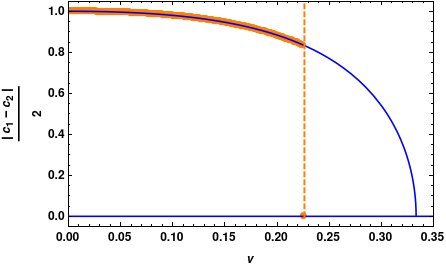
Figure 1: Absolute net concentration $\frac{1}{2}|c_{1}-c_{2}|$ versus $v$ for the frustrated system with $q=4$. Points are Monte-Carlo simulations ($N=1~{}000~{}000$, $M=2000$ large MC steps, i.e., for each $v$ we perform $2\cdot 10^{9}$ updates of the system at keep the values of $c_{1}$ and $c_{2}$). Solid lines are $2x_{0}$ and $2x_{1}$ given by Eq. (10), while the dashed vertical line is the critical value of $v$ from Eq. (16).

III.2 q=4

Following the described in the previous section it is possible to obtain the results for the limiting case of $T\rightarrow 0$ also for $q=4$. By using $c_{0}\rightarrow 1/2$ and rewrite $c_{1}\rightarrow 1/2+x$ substitution we arrive at

$$x\left[\frac{2-24v}{16}+(v-1)^{2}(1+2v)x^{2}-6(v-1)^{4}x^{4}\right]=0$$ (17)

characterized with the following five solutions:

$$x_{0}= 0$$

$$x_{1,2}= \pm\frac{\sqrt{-2\sqrt{v^{2}-8v+1}+2v+1}}{2\sqrt{3}(1-v)}$$

$$x_{3,4}= \pm\frac{\sqrt{2\sqrt{v^{2}-8v+1}+2v+1}}{2\sqrt{3}(1-v)}$$ (18)

The above set of equations is a typical example of a system with hysteresis: as long as $v<1/12$ there are only three real solutions ($x_{0}$, $x_{3}$ and $x_{4}$) in the range of $v\in[1/12,4-\sqrt{15}]$ all five solutions are real, and once $v>4-\sqrt{15}$ only $x=0$ exists (see solid lines in Fig. 2). However, once again, to find the critical value of $v$ one needs to follow linear stability analysis. In this case matrix $\mathbf{L}$ reads

$$\mathbf{L}=\left(\begin{array}[]{ccc}-\frac{3}{v-2}-\frac{23}{8}&\frac{3(v-1)}{2(v-2)}&\frac{3(v-1)}{2(v-2)}\\ u&w&0\\ u&0&w\\ \end{array}\right)$$ (19)

where

$$u=\frac{v\left(2\left(\sqrt{(v-8)v+1}-1\right)+v\left(v+\sqrt{(v-8)v+1}-11\right)\right)}{3(v-1)}$$ (20)

$$w=\frac{1}{3}\left(-\sqrt{(v-8)v+1}-2v\left(v+\sqrt{(v-8)v+1}-8\right)-2\right)$$ (21)

The actual eigenvalues of the above matrix are much more complicated than in the $q=3$ case, however it is still possible to obtain an approximate value for $v^{*}$, namely

$$v^{*}\approx 0.1195$$ (22)

Figure 2 shows a comparison of the numerical simulations and antylitical solutions given by Eq. (18) and Eq. (22), presenting a prefect agreement of these two approaches.

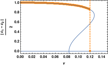
Figure 2: Absolute net concentration $\frac{1}{2}|c_{1}-c_{2}|$ versus $v$ for the frustrated system with $q=3$. Points are Monte-Carlo simulations ($N=1~{}000~{}000$, $M=2000$ large MC steps, i.e., for each $v$ we perform $2\cdot 10^{9}$ updates of the system at keep the values of $c_{1}$ and $c_{2}$). Solid lines are $2x$ given by Eq. (18), while the dashed vertical line is the critical value of $v$ from Eq. (22).

III.3 Higher values of $q$

The complexity of $\gamma_{1}^{+}-\gamma_{1}^{-}$ increases with the value of $q$. Although it is still possible to write down relevant equations, e.g., in case of $q=5$ we have

$$x\left[-6(v-1)^{5}x^{4}+5(v-1)^{3}x^{2}-\frac{1}{8}(15v-7)\right]=0$$ (23)

while for $q=6$

$$x\left[20(v-1)^{6}x^{6}-3(2v+3)(v-1)^{4}x^{4}+\right.$$

$$\left.\frac{5}{4}(v-1)^{2}(4v-1)x^{2}-\frac{3}{16}(10v-3)\right]=0,$$ (24)

nonetheless, the maximum degree of the relevant polynomial is equal to $q$ for odd values of $q$ and $q+1$ for even values. Relevant calculations, including the estimation of the largest eigenvalue of $\mathbf{L}$ become troublesome and connected to larger rounding errors. Therefore, in order to follow the behaviour of the system for larger values of $q$, it is easier to rely on numerical calculations rather than their analytical counterpart.

Figure 3 reveals a peculiar behavior of the critical value $v^{*}$ when plotted against the lobby size $q$. The oscillations have already been observed in the $q$-neigbour Ising model, both in the original paper Jedrzejewski et al. (2015) as well as inChmiel et al. (2017), however, in this case, we encounter a non-monotonical behavior of the critical value of $v$ along with $q$: both for the odd (full symbols) and even (empty symbols) we observe a clear maximum. Additionally, although initially systems with odd $q$ were characterized with larger $v^{*}$ than those with $q+1$ (i.e., for $q=3$ the symbol stays in a polarized state for larger values of $v$ than it is the case for $q=4$), after reaching $q=15$ this behavior is inverted. Finally, let us note that for sufficiently large values of $q$ the difference between odd and even values disappears

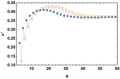
Figure 3: Critical value of $v$ versus the number of neighbors $q$. Data is Monte-Carlo simulations ($N=1~{}000~{}000$, $M=2000$ large MC steps, i.e., for each $q$ we perform $2\cdot 10^{9}$ updates of the system at keep the values of $c_{1}$ and $c_{2}$). In each case, the step of the $v$ value is equal to $\Delta v=0.001$. Full symbols reflect odd values of $q$ (starting from $q=3$) and empty symbols – even ones (starting from $q=4$). Solid lines are guides to the eye to assess the difference between consecutive values of $q$.

IV $T>0$ case

Until now we have deliberately omitted a crucial parameter of the $q$-neighbour Ising model – temperature $T$. In the case of the original model Jedrzejewski et al. (2015), the temperature is responsible for destabilizing the system; for $q\geq 3$ the system exhibits a phase transition between ferromagnetic and paramagnetic phases at a critical temperature $T^{*}$, which linearly increases with $q$. In our case it should be safe to hypothesize that the thermal noise should act in a similar way – the increase of $T$ ought to lower the value $v$ for which the system is still stable in its polarized state.

To check our assumptions we shall come back to Eq. (7) calculated for $q=3$ but this time allowing for any $T>0$. After transforming it with $c_{0}\rightarrow 1/2$ and $c_{1}\rightarrow x+1/2$ we arrive the following equation

$$\frac{3}{4}\left[1-x^{2}(v-1)^{2}\right](v-2)x\mathrm{e}^{-\frac{2}{T}}+$$

$$\frac{1}{4}\left[x^{2}(v-1)^{2}(v-4)+3v-4\right]x\mathrm{e}^{-\frac{6}{T}}+$$

$$\frac{1}{2}\left[1-3v+4(v-1)^{3}x^{2}\right]x=0$$ (25)

It is easy to see that when $T\rightarrow 0$, only the last term is kept and we obtain directly Eq. (9). Despite its complex form Eq. (25) is a simple cubic equation with respect to $x$ with one solution $x_{0}=0$ and the other two being

$$x_{1,2}=\frac{\pm 1}{2(1-v)}\sqrt{\frac{(4-3v)\mathrm{e}^{-\frac{6}{T}}-(v-2)\mathrm{e}^{-\frac{2}{T}}+2(3v-1)}{(v-4)\mathrm{e}^{-\frac{6}{T}}-(v-2)\mathrm{e}^{-\frac{2}{T}}+2(v-1)}}$$ (26)

At this point we can follow the procedure introduced for the $T\rightarrow 0$, case, which consists of linearization of $y^{+}_{1}-y^{-}_{1}$, $y^{+}_{2}-y^{-}_{2}$ and $y^{+}_{0}-y^{-}_{0}$, creation of the matrix of coefficients $\mathbf{L}$, and calculating the largest eigenvalue of $\mathbf{L}$. This way it is possible to obtain the critical value $v^{*}$ as a function of the temperature $v^{*}(T)$ and by plugging it into Eq. (26) – also the predicted concentration right before the collapse of polarized clusters. Due to very complex formulas, we refrain from presenting these solutions in an explicit form here. Figure 4 presents a comparison of these predictions with the data obtained directly from Monte-Carlo simulations for different values of $T$. As expected, an increase in $T$ results in a decrease in the critical value of $v$ needed to destroy polarized clusters. Let us underline here, that for a sufficiently large value of $T$ (e.g., $T=1.6$) the observed net concentration drops down to rather low levels.

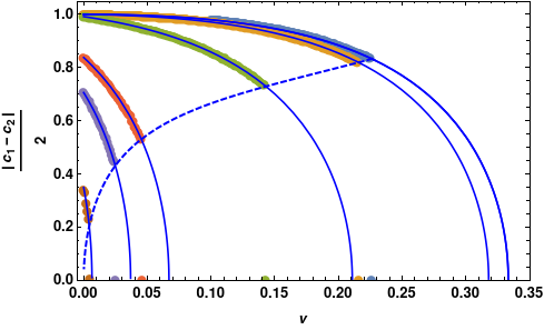
Figure 4: Absolute net concentration $\frac{1}{2}|c_{1}-c_{2}|$ versus $v$ for $q=3$ and different values of $T$ (right to left: $T=0$, $T=0.5$, $T=1.0$, $T=1.5$, $T=1.6$ and $T=1.7$). Points are Monte-Carlo simulations ($N=1~{}000~{}000$, $M=2000$ large MC steps, i.e., for each $v$ we perform $2\cdot 10^{9}$ updates of the system at keep the values of $c_{1}$ and $c_{2}$). Solid lines are $2x_{1}$ given by Eq. (26), while the dashed line comes from inserting the obtain function $v^{*}(T)$ into Eq. (26).

V Conclusions

In this paper, we have examined the interplay between the lobby size $q$ in the $q$-neighbor Ising model and the level of overlap of two fully connected graphs. Results suggest that for each lobby size $q\geq 3$ there exists a specific level of overlap $v^{*}$ which destroys initially polarized clusters of opinions. However, the dependence of the $v^{*}$ on the lobby size $q$ is far from trivial, showing a clear maximum that additionally depends on the parity of $q$. The temperature is a destructive factor, its increase leads to the earlier collapse of polarized clusters but it additionally brings a substantial decrease in the polarization.

Appendix

If $q=1$, we arrive at

$$-x\left[2+\left(\mathrm{e}^{2/T}-1\right)v\right]=0,$$ (27)

with only solution $x=0$, for any value $v$ and $T$.
 
In case $q=2$ we obtain

$$\frac{1}{2}\mathrm{e}^{-4/T}x\left[-3+2v-\mathrm{e}^{-4/T}(1+2v)+4(\mathrm{e}^{4/T}-1)(v-1)^{2}x^{2})\right]=0,$$ (28)

with three solutions

$$x_{0}~{}~{} =~{}0$$

$$x_{1,2} =\pm\frac{1}{2(v-1)}\sqrt{\frac{3+\mathrm{e}^{4/T}-2v(\mathrm{e}^{4/T}-1)}{\mathrm{e}^{4/T}-1}}.$$ (29)

However, as $x_{1}>\frac{1}{2}$ and $x_{2}<-\frac{1}{2}$ for any values of $v$ and $T$ the only physical solution is $x=0$.

References

- Jedrzejewski et al. (2015) A. Jedrzejewski, A. Chmiel, and K. Sznajd-Weron, Phys. Rev. E 92, 052105 (2015).
- Nyczka et al. (2012) P. Nyczka, K. Sznajd-Weron, and J. Cisło, Phys. Rev. E 86, 011105 (2012).
- Chmiel et al. (2017) A. Chmiel, J. Sienkiewicz, and K. Sznajd-Weron, Physical Review E 96 (2017), 10.1103/PhysRevE.96.062137.
- Chmiel and Sznajd-Weron (2015) A. Chmiel and K. Sznajd-Weron, Phys. Rev. E 92, 052812 (2015).
- Chmiel et al. (2020) A. Chmiel, J. Sienkiewicz, A. Fronczak, and P. Fronczak, Entropy 22 (2020), 10.3390/e22091018.
- DiMaggio et al. (1996) P. DiMaggio, J. Evans, and B. Bryson, American journal of Sociology 102, 690 (1996).
- McCright and Dunlap (2011) A. M. McCright and R. E. Dunlap, The Sociological Quarterly 52, 155 (2011).
- Mouw and Sobel (2001) T. Mouw and M. E. Sobel, American Journal of Sociology 106, 913 (2001).
- Lambiotte et al. (2007) R. Lambiotte, M. Ausloos, and J. Hołyst, Physical Review E 75, 030101 (2007).
- Baumann et al. (2020) F. Baumann, P. Lorenz-Spreen, I. M. Sokolov, and M. Starnini, Physical Review Letters 124 (2020), 10.1103/physrevlett.124.048301.
- Gajewski et al. (2022) L. G. Gajewski, J. Sienkiewicz, and J. A. Hołyst, Phys. Rev. E 105, 024125 (2022).
- Lambiotte and Ausloos (2007) R. Lambiotte and M. Ausloos, Journal of Statistical Mechanics: Theory and Experiment 2007, P08026 (2007).