Minimal Sparsity for Second-Order Moment-SOS Relaxations
of the AC-OPF Problem

Abstract

AC-OPF (Alternative Current Optimal Power Flow) aims at minimizing the operating costs of a power grid under physical constraints on voltages and power injections. Its mathematical formulation results in a nonconvex polynomial optimization problem which is hard to solve in general, but that can be tackled by a sequence of SDP (Semidefinite Programming) relaxations corresponding to the steps of the moment-SOS (Sums-Of-Squares) hierarchy. Unfortunately, the size of these SDPs grows drastically in the hierarchy, so that even second-order relaxations exploiting the correlative sparsity pattern of AC-OPF are hardly numerically tractable for large instances — with thousands of power buses. Our contribution lies in a new sparsity framework, termed minimal sparsity, inspired from the specific structure of power flow equations. Despite its heuristic nature, numerical examples show that minimal sparsity allows the computation of highly accurate second-order moment-SOS relaxations of AC-OPF, while requiring far less computing time and memory resources than the standard correlative sparsity pattern. Thus, we manage to compute second-order relaxations on test cases with about 6000 power buses, which we believe to be unprecedented.

Nomenclature

• For a finite set $F$, we write $|F|$ for its cardinality.

• For a complex number $z\in\mathbb{C}$, we write $\angle z$ for its angle; $|z|$ for its magnitude; $z^{*}$ for its complex conjugate; $\Re(z)$ for its real part; and $\Im(z)$ for its imaginary part.

• For a pair of integers $(a,b)\in\mathbb{N}^{2}$ with $a\leq b$, we write $\left\llbracket a,b\right\rrbracket$ for the sequence $\{a,a+1,\ldots,b\}$.

• For an $N\times N$ real symmetric matrix $M\in\mathbb{S}^{N}$, $M\succeq 0$ means that $M$ is positive semidefinite (PSD).

• For real matrices $(A,B)\in(\mathbb{R}^{N\times N})^{2}$, we write $\left\langle A\>,B\right\rangle$ for the Frobenius inner product between $A$ and $B$.

• For a polynomial function $f:\mathbb{R}^{N}\to\mathbb{R}$ that decomposes as $\sum_{\alpha\in\mathbb{N}^{N}}f_{\alpha}x^{\alpha}$ in the standard monomial basis, we denote its support by $\text{supp}(f)=\left\{\alpha\in\mathbb{N}^{N}\>\left|\>f_{\alpha}\neq 0\right.\right\}$, and the set of variables involved in $f$ by $\text{var}(f)=\left\{n\in\left\llbracket 1,N\right\rrbracket\>\left|\>\exists\alpha\in\text{supp}(f)\;,\enspace\alpha_{n}\neq 0\right.\right\}$.

Whether $|\cdot|$ denotes cardinality or magnitude is always clear from context.

I Introduction

The AC-OPF (Alternative Current - Optimal Power Flow) problem plays a central role for the management of AC power grids, but remains highly challenging to solve. Indeed, AC-OPF formulates as a nonconvex optimization program, and real scale instances typically have thousands of decision variables [1]. A common way of addressing this problem is to compute a local solution with a nonlinear solver, but the solution obtained might not be globally optimal [2]. Therefore, a vast body of literature have concentrated on relaxations of the original problem to compute lower bounds so as to estimate the quality of a local solution. We refer to [3] for a recent survey of such relaxations.

In this paper, we follow the approach of [4, 5] to compute lower bounds of AC-OPF instances based on the moment-SOS (Sums-Of-Squares) hierarchy [6]. In this framework, we consider a sequence of SDP (Semidefinite Programming) relaxations of the AC-OPF problem, whose values converge monotonously to the optimal value of the original problem. This sequence generically converges in a finite number of steps [7] and, experimentally, the second-order relaxation already achieves this convergence for most of the AC-OPF test cases reported in [4, 5, 8]. However, the size of the SDPs involved in the hierarchy grows drastically with the number of AC-OPF variables and with the order of the relaxation, so that this method becomes rapidly challenging from a numerical perspective.

Exploiting the correlative sparsity pattern [9] of AC-OPF has led to a hierarchy of SDP relaxations of reduced size, and has helped a lot to scale to larger networks [10]. See also the recent survey [11] for several applications of sparse polynomial optimization. Yet, even these sparse second-order relaxations yield out-of-memory errors for some instances with about a hundred of power buses on a computer with 125 GB of RAM [8]. Regarding instances with thousands of buses, the most scalable approach to our knowledge seems to be the recent correlative-term sparsity framework [12], which enables the computation of partial sparse second-order moment relaxations for large scale power grids [13]. Nevertheless, the accuracy of second-order relaxations remains attractive, as it provides lower bounds certifying 0.00% of optimality gaps on almost all tractable instances of [8].

Contribution: we focus our attention on sparse second-order moment-SOS relaxations of AC-OPF based on correlative sparsity. In the standard case, the size of the matrix variables involved is ruled by a family of subsets of optimization variables obtained by an algorithmic routine — computing the maximal cliques of a chordal graph. This approach enforces the RIP (Running Intersection Property), which ensures the convergence of the sparse hierarchy. We refer to [14] for technical details, including the formal definition of the RIP.

Our contribution lies in a new sparsity framework, that we call minimal sparsity. Compared with the standard approach, we chose to relax the RIP so as to gain control on the size of matrix variables. Our definition of minimal sparsity is inspired by the specific structure of the power flow equations and results in sparse second-order relaxations that have smaller matrix variables — which is generally preferred by SDP solvers based on interior-point methods [15]. Therefore, our approach is heuristic — as we relax the RIP, convergence to the global minimum is not guaranteed any more — although we may still easily extract a global optimal solution of AC-OPF if the moment matrices of our relaxations are rank-one. In spite of this heuristic nature, we report that minimal sparsity yields highly accurate lower bounds on practical test cases. Moreover, the second-order relaxations obtained scale much better than their clique-based counterparts, allowing us to handle AC-OPF instances with thousands of buses.

The paper is organized as follows. First, in §II, we recall background notions on sparse moment-SOS hierarchies and their application to AC-OPF. Second, in §III, we introduce our new minimal sparsity framework. Third, in §IV, we illustrate the strengths of minimal sparsity by computing second-order moment-SOS relaxations of the AC-OPF problem on various numerical test cases.

II Sparse moment-SOS relaxations for the AC-OPF problem

First, in §II-A, we recall the formulation of the AC-OPF problem. Second, in §II-B, we review basic concepts of moment-SOS hierarchies and their applications to certify global optimality in AC-OPF. Third, in §II-C, we present background notions on sparse moment-SOS relaxations.

II-A The AC-OPF problem

In the AC-OPF problem, we aim at minimizing the operating costs of a power grid while satisfying power flow balance equations and infrastructure constraints. We model the grid by a directed graph $(\mathcal{B},\mathcal{L})$ where nodes $\mathcal{B}$ represent buses and edges $\mathcal{L}$ represent power lines. Line orientations model the asymmetry of power flow along transmission lines in AC power grids. A subset $\mathcal{G}\subseteq\mathcal{B}$ of nodes highlights buses with generating power units. An illustrative $(\mathcal{B},\mathcal{L})$ example based on PGLib’s case 14 IEEE is given in Figure 1.

Figure 1: Example of $(\mathcal{B},\mathcal{L})$ graph model for PGLib’s case 14 IEEE: nodes represent buses and edges represent power lines with their conventional power flow orientation. Red circle node markers highlight buses with power generators.

For the sake of clarity, we assume here that at most one single line can connect two buses $(i,j)\in\mathcal{B}^{2}$. Parallel lines can be modeled by adequate edge labeling as in [1, Model 1].

Formally, AC-OPF amounts to solving the following optimization problem:

$$\min_{\begin{subarray}{c}v\in\mathbb{C}^{|\mathcal{B}|}\\ s\in\mathbb{C}^{|\mathcal{G}|}\\ s^{\ell}\in\mathbb{C}^{2|\mathcal{L}|}\end{subarray}}\quad\sum_{g\in\mathcal{G}}C_{2,g}\Re(s_{g})^{2}+C_{1,g}\Re(s_{g})+C_{0,g}\;,$$ (1a)

s.t.

$$\forall i\in\mathcal{B}_{\text{ref}}\;,\enspace\angle v_{i}=0\;;$$ (1b)

$$\forall g\in\mathcal{G}\;,\enspace\underline{S}_{g}\leq s_{g}\leq\overline{S}_{g}\;;$$ (1c)

$$\forall i\in\mathcal{B}\;,$$

$$\underline{V}_{i}\leq|v_{i}|\leq\overline{V}_{i}\;,$$ (1d)

$$\sum_{g\in\mathcal{G}(i)}s_{g}-L_{i}-\big{(}Y^{\text{s}}_{i}\big{)}^{*}|v_{i}|^{2}=\sum_{j\in\mathcal{N}(i)}s^{\ell}_{i,j}\;;$$ (1e)

$$\forall(i,j)\in\mathcal{L}\;,$$

$$s^{\ell}_{i,j}=\big{(}Y_{i,j}+Y_{i,j}^{c}\big{)}^{*}\frac{|v_{i}|^{2}}{|{}_{i,j}|^{2}}-Y_{i,j}^{*}\frac{v_{i}v_{j}^{*}}{{}_{i,j}}\;,$$ (1f)

$$s^{\ell}_{j,i}=\big{(}Y_{i,j}+Y_{j,i}^{c}\big{)}^{*}|v_{j}|^{2}-Y_{i,j}^{*}\frac{v_{i}^{*}v_{j}}{{}_{i,j}^{*}}\;,$$ (1g)

$$|s^{\ell}_{i,j}|\leq\overline{S}_{i,j}\;,\enspace|s^{\ell}_{j,i}|\leq\overline{S}_{i,j}\;,$$ (1h)

$$\underline{\Theta}_{i,j}\leq\angle(v_{i}v_{j}^{*})\leq\overline{\Theta}_{i,j}\;.$$ (1i)

In the above formulation, lower case letters are used for decision variables and capital letters refer to constant parameters. The original decision variables are the bus voltages $v=\{v_{i}\}_{i\in\mathcal{B}}$ and the power generation values $s=\{s_{g}\}_{g\in\mathcal{G}}$. Additionally, for every edge $(i,j)\in\mathcal{L}$, we introduce $s^{\ell}_{i,j}$ for the power flow from bus $i$ to bus $j$ and $s^{\ell}_{j,i}$ for the power flow from bus $j$ to bus $i$.

We now provide physical interpretations for the objective and constraints of Problem (1):

• We minimize power generation costs (1a), which are assumed to only depend on the real part of $s_{g}$, for $g\in\mathcal{G}$ — that is, on active power generation — with parameters $(C_{0,g},C_{1,g},C_{2,g})\in\mathbb{R}^{3}$.

• In constraint (1b), we set the voltage angle of some reference buses $\mathcal{B}_{\text{ref}}\subseteq\mathcal{B}$ to zero to address the rotational invariance of voltage solutions.

• In constraints (1c)-(1d), we impose bounds $(\underline{S}_{g},\overline{S}_{g})\in\mathbb{C}^{2}$ on the real and imaginary parts of the generated power $s_{g}$, for $g\in\mathcal{G}$, and bounds $(\underline{V}_{i},\overline{V}_{i})\in\mathbb{R}^{2}_{+}$ on the magnitude of the bus voltage $v_{i}$, for $i\in\mathcal{B}$.

• In constraint (1e), we enforce the balance of power flows at every bus $i\in\mathcal{B}$. The balance equation involves power generations $s_{g}$ for $g$ in the (possibly empty) set $\mathcal{G}(i)\subseteq\mathcal{G}$ of generators at bus $i$; power flows $s^{\ell}_{i,j}$ for $j$ in the set $\mathcal{N}(i)\subseteq\mathcal{B}$ of neighbors of bus $i$; the load $L_{i}\in\mathbb{C}$ and a shunt admittance term with $Y^{\text{s}}_{i}\in\mathbb{C}$.

• In constraints (1f)-(1g), we give the expression of power flows ($s^{\ell}_{i,j},s^{\ell}_{j,i}$) along every line $(i,j)\in\mathcal{L}$, following the $\Pi$-circuit branch model with parameters $(Y_{i,j},Y_{i,j}^{c},Y_{j,i}^{c},{}_{i,j})\in\mathbb{C}^{4}$ detailed in [1, Appendix B].

• In constraints (1h)-(1i), we impose a thermal limit $\overline{S}_{i,j}\in\mathbb{R}_{+}$ on power flows and voltage angle difference bounds $(\underline{\Theta}_{i,j},\overline{\Theta}_{i,j})\in\mathbb{R}^{2}$ for every line $(i,j)\in\mathcal{L}$.

Due to nonlinear equality and nonconvex inequality constraints, Problem (1) is nonconvex, and hard to solve in general [16].

II-B SDP lower bounds via moment-SOS hierarchies

Following the approach of [4, 5], AC-OPF can be cast as a POP (Polynomial Optimization Problem) to benefit from powerful results of the moment-SOS hierarchy. We introduce notations for such a reformulation of Problem (1) and recall some fundamental properties of moment-SOS relaxations.

From AC-OPF to POP

by considering separately the real and imaginary parts of voltage and power generation variables of Problem (1), we obtain ${N}=2(|\mathcal{B}|+|\mathcal{G}|)$ real variables $x\in\mathbb{R}^{N}$ (power flow variables are omitted by injecting (1f)-(1g) into (1e)). The correspondence between AC-OPF and POP variables is formalized by two bijective mappings

$${\mathfrak{b}^{\text{r}}}:\mathcal{G}\cup\mathcal{B}\to\left\llbracket 1,\frac{{N}}{2}\right\rrbracket\;,\enspace{\mathfrak{b}^{\text{im}}}:\mathcal{G}\cup\mathcal{B}\to\left\llbracket\frac{{N}}{2}+1,{N}\right\rrbracket\;,$$ (2a)

so that

$$x_{{\mathfrak{b}^{\text{r}}}(g)} =\Re(s_{g})\;,\enspace x_{{\mathfrak{b}^{\text{im}}}(g)}=\Im(s_{g})\;,\enspace\forall g\in\mathcal{G}\;,$$ (2b)

$$x_{{\mathfrak{b}^{\text{r}}}(i)} =\Re(v_{i})\;,\enspace x_{{\mathfrak{b}^{\text{im}}}(i)}=\Im(v_{i})\;,\enspace\forall i\in\mathcal{B}\;.$$ (2c)

Then, we observe that every constraint in (1b)-(1i) can be equivalently formulated as an equality or inequality constraint defined with a multivariate polynomial in $x\in\mathbb{R}^{N}$. To perform this reformulation, constraints (1d) and (1h) need to be squared and constraint (1i) needs to be transformed as detailed e.g. in [17, §5.1.2]. Thus, by introducing ${K}+1$ appropriate real multivariate polynomial functions $\{f_{k}\}_{k\in\left\llbracket 0,{K}\right\rrbracket}$, Problem (1) can be written as a POP:

$$\rho =\min_{x\in\mathcal{X}}f_{0}(x)\;,\enspace\text{ where }\enspace$$ (3a)

$$\mathcal{X} =\left\{x\in\mathbb{R}^{N}\>\left|\>f_{k}(x)\geq 0\;,\enspace\forall k\in\left\llbracket 1,{K}\right\rrbracket\right.\right\}\;.$$ (3b)

The Moment-SOS hierarchy

despite its potential nonconvexity, the optimal value of Problem (3) can be approximated — and often exactly computed — by the moment-SOS hierarchy [6]. In this framework, we consider two sequences of SDPs, starting from a minimal order $r_{0}=\max\{d_{k}\}_{k\in\left\llbracket 0,K\right\rrbracket}$ where $d_{k}=\big{\lceil}\frac{\text{deg}(f_{k})}{2}\big{\rceil}$. The moment hierarchy is defined by a sequence of SDPs indexed by $r\in\left\llbracket r_{0},+\infty\right\rrbracket$:

$$\rho_{r}= \min_{y}\quad\sum_{\alpha\in\text{supp}(f_{0})}f_{0,\alpha}y_{\alpha}\;,$$ (4a)

s.t. $$M_{r}(y)\succeq 0\;,$$ (4b)

$$M_{r-d_{k}}(f_{k}y)\succeq 0\;,\enspace\forall k\in\left\llbracket 1,{K}\right\rrbracket\;,$$ (4c)

$$y_{\textbf{0}}=1\;.$$ (4d)

The entries of the so-called pseudo-moment variable vector $y$ in Problem (4) are indexed by elements of the truncated monomial basis $\{x^{\alpha}\}_{\alpha\in\mathbb{N}_{2r}^{N}}$, where $\mathbb{N}_{r}^{N}=\big{\{}\alpha\in\mathbb{N}^{N}\ |\ \sum_{n\in\left\llbracket 1:{N}\right\rrbracket}\alpha_{n}\leq r\big{\}}$ for $r\in\mathbb{N}$. Subsequently, the moment matrix in (4b) and the localization matrices in (4c) are expressed as

$$M_{r}(y) =(y_{\alpha+\beta})_{\alpha,\beta\in\mathbb{N}_{r}^{N}}\;,$$ (5a)

$$M_{r-d_{k}}(f_{k}y) =\Big{(}\sum_{\gamma\in\text{supp}(f_{k})}f_{k,\gamma}y_{\alpha+\beta+\gamma}\Big{)}_{\alpha,\beta\in\mathbb{N}_{r-d_{k}}^{N}}\;.$$ (5b)

These matrices have entries that are linear in the ones of $y$, so that we can write $M_{r}(y)=\sum_{\alpha\in\mathbb{N}_{2r}^{N}}A_{0,\alpha}y_{\alpha}$ and $M_{r-d_{k}}(f_{k}y)=\sum_{\alpha\in\mathbb{N}_{2r}^{N}}A_{k,\alpha}y_{\alpha}$ by introducing adequate matrices $\{A_{k,\alpha}\}_{\alpha\in\mathbb{N}_{2r}^{N}}$ for all $k\in\left\llbracket 0,{K}\right\rrbracket$.

By considering the dual of (4), we obtain the SOS hierarchy of SDPs indexed by $r\in\left\llbracket r_{0},+\infty\right\rrbracket$:

$$\theta_{r}= \max_{G,t}\quad t\;,$$ (6a)

s.t. $$f_{0,\textbf{0}}-t=\sum_{k\in\left\llbracket 0,{N}\right\rrbracket}\left\langle A_{k,\textbf{0}}\>,G_{k}\right\rangle\;,$$ (6b)

$$f_{0,\alpha}=\sum_{k\in\left\llbracket 0,{N}\right\rrbracket}\left\langle A_{k,\alpha}\>,G_{k}\right\rangle\;,\enspace\forall\alpha\in\mathbb{N}_{2r}^{N}\setminus\{\textbf{0}\}\;,$$ (6c)

$$G_{k}\succeq 0\;,\enspace\forall k\in\left\llbracket 0,K\right\rrbracket\;.$$ (6d)

In the context of AC-OPF, strong duality holds between Problems (4) and (6) (see [4]), and the nondecreasing sequences of lower bounds $\{\rho_{r}\}_{r\geq r_{0}}$ and $\{\theta_{r}\}_{r\geq r_{0}}$ converge to the value $\rho$ of the POP (3) (see [6]). However, the sizes of the corresponding SDP relaxations grow drastically with the values of ${N}$ and $r$, as the largest Gram matrix $G_{0}$ in (6) and the moment matrix $M_{r}(y)$ in (4) are of size $|\mathbb{N}_{r}^{N}|=\binom{{N}+r}{r}$.

II-C Sparse relaxations

One way to bypass the curse of dimensionality mentioned hereabove is to exploit the sparsity of AC-OPF, as initially suggested in [10]. In the context of the moment hierarchy, sparsity consists in reducing the dimension of the search space of Problem (4) by selecting a subset of monomials in $\{x^{\alpha}\}_{\alpha\in\mathbb{N}_{2r}^{N}}$ for indexing the pseudo-moment variable vector $y$. We concentrate on the correlative sparsity pattern [9] which introduces a hierarchy of sparse moment relaxations:

$$\rho_{r}(\mathcal{I})= \min_{y}\quad\sum_{\alpha\in\text{supp}(f_{0})}f_{0,\alpha}y_{\alpha}\;,$$ (7a)

s.t. $$M_{r}(y;\mathcal{I}_{p})\succeq 0\;,\enspace\forall p\in\left\llbracket 1,{P}\right\rrbracket\;,$$ (7b)

$$M_{r-d_{k}}(f_{k}y;\mathcal{I}_{p})\succeq 0\;,\enspace\forall k\in\mathcal{K}_{p}\;,\enspace$$ (7c)

$$\vspace{3cm}\forall p\in\left\llbracket 1,{P}\right\rrbracket\;,$$

$$y_{\textbf{0}}=1\;.$$ (7d)

Problem (7) is parameterized by a family of subsets of $\left\llbracket 1,{N}\right\rrbracket$, denoted $\mathcal{I}=\{\mathcal{I}_{p}\}_{\in\left\llbracket 1,{P}\right\rrbracket}$, and satisfying $\cup_{p\in\left\llbracket 1,{P}\right\rrbracket}\mathcal{I}_{p}=\left\llbracket 1,{N}\right\rrbracket$. The constraints $\{f_{k}\}_{k\in\left\llbracket 1,{K}\right\rrbracket}$ are distributed over a partition $\{\mathcal{K}_{p}\}_{\in\left\llbracket 1,{P}\right\rrbracket}$ of $\left\llbracket 1,{K}\right\rrbracket$ such that for all $p\in\left\llbracket 1,{P}\right\rrbracket$ and $k\in\mathcal{K}_{p}$, $\text{var}(f_{k})\subseteq\mathcal{I}_{p}$. Then, for $p\in\left\llbracket 1,{P}\right\rrbracket$, the sparse moment and localization matrices in (7b)-(7c) are defined after (5) by selecting only rows and columns indexed by monomials in $\{x^{\alpha}\}_{\alpha\in\mathbb{N}_{2r}^{N}}$ satisfying $\text{var}(x^{\alpha})\subseteq\mathcal{I}_{p}$. Naturally, the dual of Problem (7) gives rise to a sparse SOS hierarchy, whose sequence of bounds is introduced as $\{\theta_{r}(\mathcal{I})\}_{r\geq r_{0}}$.

We remind that the choice of the subsets $\mathcal{I}$ is of paramount importance. On the practical side, the cardinalities of these subsets control the sizes of the matrices in (7b)-(7c). In general, the smaller these matrices, the better the numerical performances of SDP solvers, especially for those based on interior-point methods [15]. On the theoretical side, the bounds $\{\rho_{r}(\mathcal{I})\}_{r\geq r_{0}}$ are not guaranteed to converge to the value $\rho$ of the POP (3) for any choice of $\mathcal{I}$. The most favorable case is when the subsets $\mathcal{I}$ satisfy the RIP (Running Intersection Property) where asymptotic convergence is preserved [14]. These considerations on the design of $\mathcal{I}$ are further investigated in the next section.

III Minimal sparsity for scalable AC-OPF relaxations

We recall basic notions of clique-based sparsity and expose some of its limitations regarding computing scalability in  §III-A. As an alternative, we introduce our minimal sparsity pattern in §III-B. We further detail a method to control the cardinalities of the subsets $\mathcal{I}$ in §III-C.

III-A Clique-based sparsity and its limitations

We recall how to compute clique-based subsets $\mathcal{I}$ and discuss some limitations of this approach.

Clique-based subsets

the design of subsets $\mathcal{I}$ satisfying the RIP is usually based on the following algorithmic routine.

• First, we define the correlative sparsity pattern graph $(\mathcal{V},\mathcal{E})$. In this graph, nodes $\mathcal{V}$ represent the ${N}$ variables of the POP (3) and undirected edges $\mathcal{E}$ account for products between variables in the polynomial functions $\{f_{k}\}_{k\in\left\llbracket 1,{K}\right\rrbracket}$: an edge $(n_{1},n_{2})\in\mathcal{E}$ indicates that there exists $\alpha\in\cup_{k\in\left\llbracket 0,{K}\right\rrbracket}\text{supp}(f_{k})$ such that $\{n_{1},n_{2}\}\subseteq\text{var}(x^{\alpha})$.

• Second, we perform a chordal extension of $(\mathcal{V},\mathcal{E})$. We recall that a graph is chordal if each of its cycle of length four ou greater has a chord. Therefore, chordal extension adds new edges, resulting in a new graph $(\mathcal{V},\overline{\mathcal{E}})$, where $\mathcal{E}\subseteq\overline{\mathcal{E}}$.

• Third, we define subsets $\mathcal{I}^{\text{c}}$ as the maximal cliques of the chordal graph $(\mathcal{V},\overline{\mathcal{E}})$. We recall that a clique is a complete subgraph of $(\mathcal{V},\overline{\mathcal{E}})$, and that it is maximal when it cannot be augmented by adding an adjacent node.

The clique-based subsets $\mathcal{I}^{\text{c}}$ satisfy the RIP, and thus ensure the convergence of the correlative sparse moment-SOS hierarchy [14].

Limitations of clique-based sparsity

the above routine for designing the subsets $\mathcal{I}$ gives a systematic way to reduce the computing burden of the dense relaxation (4). However, for large AC-OPF instances, even the sparse relaxation (7) can be numerically challenging. Experimentally, [8] report that the second-order sparse moment relaxation triggers an out-of-memory error on a computer allowed with 125 GB of RAM for PGLib’s instances 89 Pegase and 162 IEEE.

Therefore, some works concentrate on improving the algorithmic routine $(i)-(iii)$ to reduce memory usage and computing time for solving (7). In particular, [18, 19] propose clique merging strategies as a post-processing of $(iii)$. This line of work has allowed up to $\times$3 decreases in solving time for first-order relaxations [18]. However, extensions to second-order relaxations seem much less effective [20, §4.5]. We believe that it is due to the iteration complexity of interior-point SDP solvers, which typically perform operations that scale cubically with the size of the largest SDP matrix [15]. We recall that the largest matrix in (7) is of size

$$\binom{m+r}{r}\;,\enspace\text{ where }m=\max_{p\in\left\llbracket 1,{P}\right\rrbracket}|\mathcal{I}_{p}|\;,$$ (8)

hence the importance of moderating the cardinalities of the subsets in $\mathcal{I}$ to alleviate memory requirements and computing time in second-order sparse relaxations. Clearly, a clique merging strategy is not meant to reduce these cardinalities, and therefore does not address what we identify as the principal bottleneck in second-order sparse relaxations.

III-B Minimal sparsity

We introduce minimal subsets $\mathcal{I}^{\text{m}}$ to address the principal limitations faced with clique-based sparsity in AC-OPF. Our definition builds on the specific structure of power flow equations: for each bus $i\in\mathcal{B}$, we select the minimal group of POP variables required to write the power flow balance equation at bus $i$. This results in ${P}=|\mathcal{B}|$ subsets given by

$$\mathcal{I}^{\text{m}}_{\#i}= \{{\mathfrak{b}^{\text{r}}}(i),{\mathfrak{b}^{\text{im}}}(i)\}\bigcup_{j\in\mathcal{N}(i)}\{{\mathfrak{b}^{\text{r}}}(j),{\mathfrak{b}^{\text{im}}}(j)\}$$

$$\bigcup_{g\in\mathcal{G}(i)}\{{\mathfrak{b}^{\text{r}}}(g),{\mathfrak{b}^{\text{im}}}(g)\}\;,$$ (9a)

where, assuming an arbitrary order on buses $$\mathcal{B} \#i\in\left\llbracket 1,{P}\right\rrbracket i\in\mathcal{B}$$, we denote by the position of bus . In term of correspondence between POP and AC-OPF formulations, we obtain the following relationship:

$$\{x_{n}\}_{n\in\mathcal{I}^{\text{m}}_{\#i}}= \{\Re(v_{i}),\Im(v_{i})\}\bigcup_{j\in\mathcal{N}(i)}\{\Re(v_{j}),\Im(v_{j})\}$$

$$\bigcup_{g\in\mathcal{G}(i)}\{\Re(s_{g}),\Im(s_{g})\}\;.$$ (9b)

The above expression highlights that in $\mathcal{I}^{\text{m}}_{\#i}$, we select the minimal amount of AC-OPF variables that we need to write constraints (1e) and (1f)-(1g) at bus $i\in\mathcal{B}$ for Problem (1).

Minimal sparsity entails a trade-off between the number of subsets in $\mathcal{I}$ and their cardinalities. We illustrate this trade-off by comparing clique-based subsets $\mathcal{I}^{\text{c}}$ and minimal subsets $\mathcal{I}^{\text{m}}$ for PGLib’s case 162 IEEE. We compute the chordal extension $(\mathcal{V},\overline{\mathcal{E}})$ and its maximal cliques using the greedy fillin heuristic implemented in the TSSOS package [21], as this heuristic is expected to yield smaller average clique numbers than other standard heuristics [22]. The histogram of the cardinalities of sets for both sparsity patterns is given in Figure 2. For case 162 IEEE, $\mathcal{I}^{\text{c}}$ has ${P}=126$ sets, the largest of which has 70 variables, whereas $\mathcal{I}^{\text{m}}$ has ${P}=162$ sets with at most 22 variables. Consequently, the sparse moment-SOS relaxations written with $\mathcal{I}^{\text{m}}$ have a larger amount of PSD constraints-matrices than clique-based relaxations, but their dimensions are much smaller. In general, this situation is preferred by SDP solvers based on interior-point methods [15].

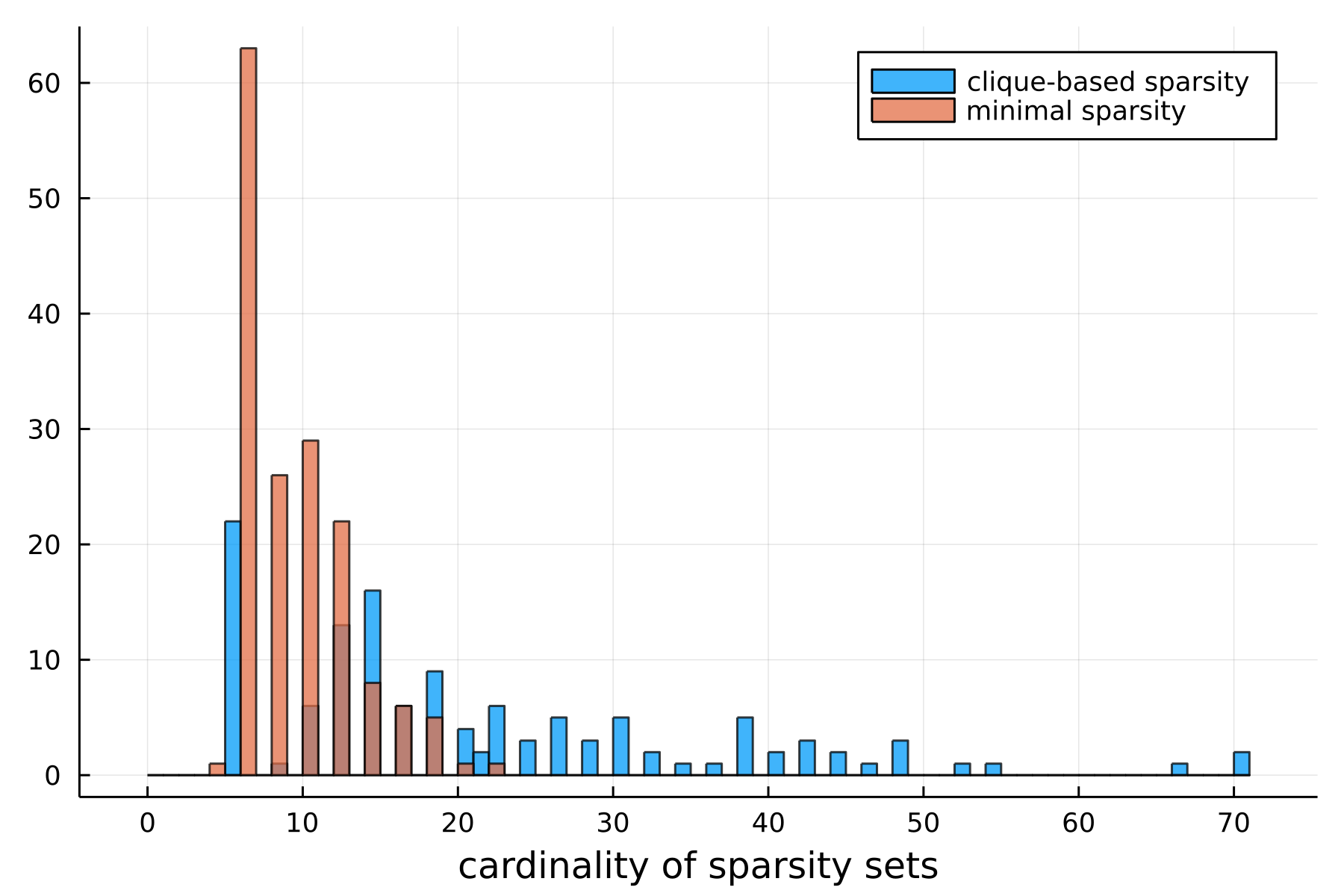
Figure 2: Histogram of the cardinalities of clique-based subsets $\mathcal{I}^{\text{c}}$ (blue color) and minimal subsets $\mathcal{I}^{\text{m}}$ (red color) for PGLib’s case 162 IEEE

III-C Finer control on the size of subsets

If the graph $(\mathcal{B},\mathcal{L})$ has nodes with a high number of neighbors, the minimal subsets $\mathcal{I}^{\text{m}}$ defined by (9a) may still have large cardinalities. Assuming that we wish to impose a maximal cardinality threshold $\bar{I}$ for the subsets $\mathcal{I}^{\text{m}}$, we propose a modification of the AC-OPF Problem (1) and of the minimal subsets $\mathcal{I}^{\text{m}}$ to meet this requirement.

In our approach, when $|\mathcal{I}^{\text{m}}_{\#i}|>\bar{I}$ at some bus $i\in\mathcal{B}$, we split neighboring buses $\mathcal{N}(i)$ into a partition $\{\mathcal{N}_{a}(i)\}_{a\in\mathcal{A}(i)}$, where the set $\mathcal{A}(i)$ is introduced to index additional complex variables $\{z^{\ell}_{i,a}\}_{a\in\mathcal{A}(i)}$ for the AC-OPF Problem (1). Then, we rewrite the power flow equation (1e) at bus $i$ as

$$\sum_{g\in\mathcal{G}(i)}s_{g}-L_{i}-\big{(}Y^{\text{s}}_{i}\big{)}^{*}|v_{i}|^{2}=\sum_{a\in\mathcal{A}(i)}z^{\ell}_{i,a}\;,$$ (10a)

$$z^{\ell}_{i,a}=\sum_{j\in\mathcal{N}_{a}(i)}s^{\ell}_{i,j}\;,\enspace\forall a\in\mathcal{A}(i)\;,$$ (10b)

so that each constraint in (10a)-(10b) involves less variables than the original aggregated formulation (1e) — assuming that $|\mathcal{A}(i)|<|\mathcal{N}(i)|$ . Next, we add $2|\mathcal{A}(i)|$ real variables to the POP (3) and extend $\{{\mathfrak{b}^{\text{r}}},{\mathfrak{b}^{\text{im}}}\}$ so that

$$\begin{cases}{\mathfrak{b}^{\text{r}}}(a)=\Re(z^{\ell}_{i,a})\ ,\\ {\mathfrak{b}^{\text{im}}}(a)=\Im(z^{\ell}_{i,a})\ ,\end{cases}\forall a\in\mathcal{A}(i)\;.$$ (11)

Finally, we define minimal subsets in the same spirit of (9a):

$$\mathcal{I}^{\text{m}}_{\#i}= \{{\mathfrak{b}^{\text{r}}}(i),{\mathfrak{b}^{\text{im}}}(i)\}\bigcup_{a\in\mathcal{A}(i)}\{{\mathfrak{b}^{\text{r}}}(a),{\mathfrak{b}^{\text{im}}}(a)\}$$

$$\bigcup_{g\in\mathcal{G}(i)}\{{\mathfrak{b}^{\text{r}}}(g),{\mathfrak{b}^{\text{im}}}(g)\}\;,$$ (12a)

$$\mathcal{I}^{\text{m}}_{\#a}= \{{\mathfrak{b}^{\text{r}}}(i),{\mathfrak{b}^{\text{im}}}(i)\}\bigcup_{j\in\mathcal{N}_{a}(i)}\{{\mathfrak{b}^{\text{r}}}(j),{\mathfrak{b}^{\text{im}}}(j)\}$$

$$\bigcup\{{\mathfrak{b}^{\text{r}}}(a),{\mathfrak{b}^{\text{im}}}(a)\}\;,\enspace\forall a\in\mathcal{A}(i)\;.$$ (12b)

In turn, the sets $\mathcal{A}(i)$ and $\{\mathcal{N}_{a}(i)\}_{a\in\mathcal{A}(i)}$ should be designed carefully to control the cardinalities of the subsets defined by (12a)-(12b). We suggest to use the solutions of the integer program

$$\min_{(n_{\mathcal{A}},\overline{n}_{a})\in\mathbb{N}^{*2}}n_{\mathcal{A}}\quad\text{ s.t. }\begin{cases}2(\overline{n}_{a}+2)\leq\bar{I}\;,\\ n_{\mathcal{A}}\times\overline{n}_{a}\geq|\mathcal{N}(i)|\;,\end{cases}$$ (13a)

which admits

$$n_{\mathcal{A}}=\left\lceil\frac{|\mathcal{N}(i)|}{\left\lfloor\frac{\bar{I}}{2}\right\rfloor-2}\right\rceil\quad\text{ and }\quad\overline{n}_{a}=\left\lceil\frac{|\mathcal{N}(i)|}{n_{\mathcal{A}}}\right\rceil$$ (13b)

as a solution, if $\bar{I}\geq 6$. The rationale behind the formulation of Problem (13a) is that we want to minimize $n_{\mathcal{A}}=|\mathcal{A}(i)|$ so as to reduce the cardinality of $\mathcal{I}^{\text{m}}_{\#i}$ in (12a). Meanwhile, we want to dispatch neighbors equally over the partition $\{\mathcal{N}_{a}(i)\}_{a\in\mathcal{A}(i)}$, which is composed of sets whose cardinalities are at most $\overline{n}_{a}$. The constraints of Problem (13a) ensure that the subsets $\{\mathcal{I}^{\text{m}}_{\#a}\}_{a\in\mathcal{A}(i)}$ in (12b) have cardinalities lower than $\bar{I}$ (first inequality) and that the partition $\{\mathcal{N}_{a}(i)\}_{a\in\mathcal{A}(i)}$ covers $\mathcal{N}(i)$ (second inequality).

Applying the solution (13b), we obtain a reduction of the cardinality of $\mathcal{I}^{\text{m}}_{\#i}$ provided that

$$\bar{I}\geq 4+\frac{2|\mathcal{N}(i)|}{|\mathcal{N}(i)|-1}\;.$$ (14)

However, we might still have that $|\mathcal{I}^{\text{m}}_{\#i}|>\bar{I}$. In this case, we can operate a similar partitioning of $\mathcal{G}(i)$ to reduce the contribution of power generation variables $\{s_{g}\}_{g\in\mathcal{G}(i)}$ to the cardinality of $\mathcal{I}^{\text{m}}_{\#i}$ in (12a).

IV Numerical examples

We illustrate the success of minimal sparsity in computing second-order moment relaxation bounds in AC-OPF. In our experiments, we use Mosek 9.3 [23] to solve SDPs and Ipopt [24] for nonlinear programs. Both solvers are applied with their default settings. We display the results of sparse SOS relaxations, i.e. the dual of (7), as they are usually better handled than moment relaxations by Mosek [23, §7.5]. The interface between data, models and solvers is implemented with JuMP [25] and PowerModels [26]. We run experiments on a 2.10 GHz Intel CPU with 150 GB of RAM. Our code is publicly available and we use open data from [27, 1].

We measure the accuracy of a relaxation in term of its optimality gap

$$\gamma_{r}(\mathcal{I})=\frac{\bar{\rho}-\theta_{r}(\mathcal{I})}{\bar{\rho}}\times 100\;,$$ (15)

where $\bar{\rho}$ is an upper bound computed with Ipopt. First, in §IV-A, we measure the accuracy of minimal sparsity on modified case 57 IEEE instances that display large optimality gaps for first-order SOS relaxations. Second, in §IV-B, we investigate the scalability of minimal sparsity on larger PGLib instances.

IV-A Case 57 IEEE modified

We consider the 1000 modified instances generated in [27, §5.4] by drawing random linear cost parameters $\{C_{1,g}\}_{g\in\mathcal{G}}$ in (1) for case 57 IEEE from [1]. We concentrate on the ten instances displaying the largest optimality gaps at the first-order SOS relaxation. Following the formulation of [27], we adopt a simplified AC-OPF model for this experiment: limits on power lines and angle differences in (1h)-(1i) are ignored and we consider only linear costs. Since moreover case 57 IEEE has at most one generator per bus, we may consider a voltage-only formulation of Problem (1), and, for the sake of numerical stability, we scale all polynomial coefficients to $f_{k,\alpha}\in[-1,1]$.

We present numerical results obtained with clique-based sparsity in Table I and with minimal sparsity in Table II. In both cases, we report the computing time (columns 2-3) and the optimality gaps (columns 4-5) of the first- and second-order SOS relaxation bounds.

Bound accuracy

we observe that the second-order relaxation based on minimal sparsity always achieves zero optimality gap for all of the modified case 57 IEEE instances (Table II, column 5). This suggests that, despite its heuristic nature, minimal sparsity is suitable to compute tight lower bounds for AC-OPF. In turn, clique-based sparsity performs equally well for the second-order relaxation (Table I, column 5). Interestingly, for first-order sparse relaxations, the optimality gaps obtained with clique-based sparsity (Table (I), column 4) are smaller than the ones of minimal sparsity (Table (II), column 4). We also note that minimal sparsity yields more stable relaxations than clique-based sparsity for instances 84 and 829, for which the computation of $\theta_{2}(\mathcal{I}^{\text{c}})$ stopped with Mosek’s SLOW_PROGRESS termination status (Table I, column 5). Better numerical stability could arise from the fact that minimal sparsity typically features smaller SDPs than clique-based sparsity.

Computing time

the main improvement of minimal-sparsity over a clique-based approach lies in the reduction of computing time. Indeed, evaluating clique-based second-order sparse relaxation bounds $\theta_{2}(\mathcal{I}^{\text{c}})$ requires 3-6 hours of computation per instance (Table I, column 3), whereas each of their minimal sparsity counterparts $\theta_{2}(\mathcal{I}^{\text{m}})$ can be computed within one minute (Table II, column 3). We believe that this shrinkage of computing time is due to the reduction of the size of the largest subsets in $\mathcal{I}$: with clique-based sparsity, we have $\max_{p}(|\mathcal{I}^{\text{c}}_{p}|)=26$, while minimal sparsity features smaller cardinalities with $\max_{p}(|\mathcal{I}^{\text{m}}_{p}|)=14$. Lastly, we mention that this way of certifying optimality gaps also outperforms the branch-and-bound technique tested in [27], which achieves an average of $0.16\%$ optimality gap after 120 hours of computation per instance.

instances	time (s)		gap (%)
	$\theta_{1}(\mathcal{I}^{\text{c}})$	$\theta_{2}(\mathcal{I}^{\text{c}})$	$\gamma_{1}(\mathcal{I}^{\text{c}})$	$\gamma_{2}(\mathcal{I}^{\text{c}})$
84	6.88 $10^{\text{-}1}$	1.97 $10^{4}$	3.05	∗0.00
260	5.90 $10^{\text{-}1}$	1.19 $10^{4}$	1.67	0.00
267	6.54 $10^{\text{-}1}$	1.37 $10^{4}$	1.21	0.00
299	6.17 $10^{\text{-}1}$	2.23 $10^{4}$	1.92	0.00
391	5.53 $10^{\text{-}1}$	1.67 $10^{4}$	1.25	0.00
628	6.16 $10^{\text{-}1}$	1.79 $10^{4}$	6.64	0.00
683	6.80 $10^{\text{-}1}$	1.44 $10^{4}$	2.32	0.00
829	6.39 $10^{\text{-}1}$	1.98 $10^{4}$	2.00	∗0.00
868	6.43 $10^{\text{-}1}$	1.41 $10^{4}$	2.17	0.00
974	6.80 $10^{\text{-}1}$	1.45 $10^{4}$	1.92	0.00

TABLE I: Results for AC-OPF case 57 modified and clique-based subsets ($|\mathcal{I}^{\text{c}}|=38\;,\enspace\max_{p}|\mathcal{I}^{\text{c}}_{p}|=26$). In all cases, the solution returned is primal feasible. Instances for which Mosek terminated with the SLOW_PROGRESS status are marked with “$*$”

instances	time (s)		gap (%)
	$\theta_{1}(\mathcal{I}^{\text{m}})$	$\theta_{2}(\mathcal{I}^{\text{m}})$	$\gamma_{1}(\mathcal{I}^{\text{m}})$	$\gamma_{2}(\mathcal{I}^{\text{m}})$
84	1.91 $10^{\text{-}1}$	4.57 $10^{1}$	3.30	0.00
260	2.58 $10^{\text{-}1}$	4.35 $10^{1}$	1.85	0.00
267	1.86 $10^{\text{-}1}$	4.39 $10^{1}$	1.42	0.00
299	1.96 $10^{\text{-}1}$	5.67 $10^{1}$	2.06	0.00
391	1.83 $10^{\text{-}1}$	5.27 $10^{1}$	1.54	0.00
628	2.00 $10^{\text{-}1}$	5.31 $10^{1}$	6.89	0.00
683	1.95 $10^{\text{-}1}$	4.56 $10^{1}$	2.50	0.00
829	1.84 $10^{\text{-}1}$	4.28 $10^{1}$	2.21	0.00
868	1.92 $10^{\text{-}1}$	4.30 $10^{1}$	2.33	0.00
974	2.08 $10^{\text{-}1}$	5.10 $10^{1}$	2.08	0.00

TABLE II: Results for AC-OPF case 57 modified and minimal sparsity subsets ($|\mathcal{I}^{\text{m}}|=57\;,\enspace\max_{p}(|\mathcal{I}^{\text{m}}_{p}|)=14$). In all cases, the solution returned is primal feasible

IV-B Standard PGLib examples

We present further results on the standard AC-OPF formulation (1). To investigate on the scalability of the results obtained on case 57 IEEE, we consider all PGLib cases with up to 1000 buses and large scale RTE cases with thousands of buses. As larger instances tend to be less numerically stable, we scale both polynomial coefficients to $f_{k,\alpha}\in[-1,1]$ and POP variables to $x_{n}\in[0,1]$. We report the performance of second-order relaxations based on minimal sparsity in Table III. We apply a maximal cardinality threshold $\bar{I}$ = 12 as introduced in §III-C, resulting in additional POP variables (Table III, column 8).

PGLib cases	computing time (s)			$\gamma_{2}(\mathcal{I}^{\text{m}})$ gap (%)			POP variables
	TYP	API	SAD	TYP	API	SAD	added	total
3 LMBD	5.32 $10^{\text{-1}}$	9.78 $10^{\text{-1}}$	5.54 $10^{\text{-1}}$	0.00	0.00	0.00	0	12
5 PJM	7.22 $10^{0}$	9.45 $10^{0}$	5.34 $10^{0}$	0.00	∗0.07	0.00	0	20
14 IEEE	2.03 $10^{1}$	2.52 $10^{1}$	1.89 $10^{1}$	0.00	0.00	0.00	0	38
24 IEEE RTS	5.19 $10^{1}$	8.73 $10^{1}$	5.56 $10^{1}$	∗0.00	∗0.00	∗0.00	24	138
30 AS	3.04 $10^{1}$	6.26 $10^{1}$	3.26 $10^{1}$	0.00	?	0.00	8	80
30 IEEE	3.86 $10^{1}$	4.29 $10^{1}$	4.45 $10^{1}$	∗0.00	∗0.00	∗0.00	8	80
39 EPRI	2.45 $10^{1}$	2.36 $10^{1}$	2.25 $10^{1}$	0.00	∗0.16	0.00	0	98
57 IEEE	4.69 $10^{1}$	4.01 $10^{1}$	4.25 $10^{1}$	0.00	0.00	0.00	12	140
60 C	5.94 $10^{1}$	1.21 $10^{2}$	8.92 $10^{1}$	∗0.00	∗0.09	∗0.03	20	186
73 IEEE RTS	1.85 $10^{2}$	2.76 $10^{2}$	1.93 $10^{2}$	∗0.00	∗4.67	∗0.05	80	424
89 PEGASE	8.59 $10^{2}$	9.14 $10^{2}$	8.12 $10^{2}$	∗0.00	?	∗0.00	158	360
118 IEEE	2.82 $10^{2}$	4.95 $10^{2}$	3.79 $10^{2}$	∗0.00	∗9.59	∗0.05	78	422
162 IEEE DTC	9.51 $10^{2}$	1.21 $10^{3}$	1.09 $10^{3}$	∗0.70	∗0.44	∗0.41	88	436
179 GOC	2.61 $10^{2}$	3.63 $10^{2}$	2.83 $10^{2}$	∗0.04	∗0.35	∗4.08	100	516
200 ACTIV	3.33 $10^{2}$	5.06 $10^{2}$	3.15 $10^{2}$	∗0.00	∗0.00	∗0.00	48	524
240 PSERC	9.05 $10^{2}$	1.38 $10^{3}$	1.02 $10^{3}$	∗1.61	∗0.24	∗2.94	292	1058
300 IEEE	9.35 $10^{2}$	8.66 $10^{2}$	1.01 $10^{3}$	∗0.00	∗0.29	∗0.00	68	806
500 GOC	1.59 $10^{3}$	1.92 $10^{3}$	1.45 $10^{3}$	∗0.00	∗2.21	∗3.66	308	1650
588 SDET	1.08 $10^{3}$	8.50 $10^{2}$	1.15 $10^{3}$	∗0.25	?	∗0.22	106	1472
793 GOC	1.09 $10^{3}$	1.22 $10^{3}$	1.31 $10^{3}$	?	?	∗1.72	116	1896
1888 RTE	4.74 $10^{3}$	4.99 $10^{3}$	4.49 $10^{3}$	?	∗0.05	∗2.58	1048	5404
1951 RTE	4.68 $10^{3}$	5.73 $10^{3}$	4.48 $10^{3}$	∗-0.01	∗0.18	∗0.25	1076	5710
2848 RTE	6.07 $10^{3}$	8.38 $10^{3}$	6.48 $10^{3}$	?	?	?	1472	8190
2868 RTE	6.98 $10^{3}$	7.62 $10^{3}$	6.85 $10^{3}$	?	?	∗0.39	1498	8356
6468 RTE	1.27 $10^{4}$	1.92 $10^{4}$	1.49 $10^{4}$	∗0.27	?	?	3438	17172
6470 RTE	1.57 $10^{4}$	1.91 $10^{4}$	1.93 $10^{4}$	∗0.74	?	?	3478	17940
6495 RTE	1.53 $10^{4}$	1.71 $10^{4}$	1.71 $10^{4}$	?	?	?	3500	17850
6515 RTE	1.81 $10^{4}$	1.88 $10^{4}$	1.53 $10^{4}$	?	?	?	3492	17890

TABLE III: Results on standard AC-OPF instances from PGLib for second-order relaxation gaps $\gamma_{2}(\mathcal{I}^{\text{m}})$ based on minimal sparsity. The maximal cardinality threshold is set to $\bar{I}$ = 12. Instances for which Mosek terminated with the SLOW_PROGRESS status are marked with “$*$” and “$?$” indicates an UNKNOWN_RESULT_STATUS

Our results

second-order minimal sparsity relaxations successfully certify less than 1% of optimality gap for 47 of the 60 instances with up to 1000 buses (Table III, columns 5-7). For 8 other instances (with gap values in bold font), Mosek stops at a feasible point with the SLOW_PROGRESS termination status, which suggests that the accuracy of the bound $\theta_{2}(\mathcal{I}^{\text{m}})$ could be further improved. Lastly, the solver returns an UNKNOWN_RESULT_STATUS for the 5 other instances.

Addressing larger AC-OPF instances appears numerically challenging, as Mosek stops with an UNKNOWN_RESULT_STATUS for 16 out of the 24 large RTE instances (Table III, columns 5-7). Moreover, we obtain a negative gap value for case 1951 RTE TYP, which means that its bound $\theta_{2}(\mathcal{I}^{\text{m}})$ should be carefully certified.

Nevertheless, we manage to compute second-order relaxations with less than 1% of optimality gaps for instances with over 6000 buses. Remarkably, these bounds are computed within the same computing time and memory resources required to compute clique-based second-order bounds for case 57 in Table I. We believe that these results are unprecedented and encouraging, as they open new perspectives for second-order relaxations of large scale AC-OPF instances.

Comparison with other approaches

we observe that minimal sparsity drastically reduces both computing times and memory requirements compared with the clique-based sparse second-order moment relaxations reported in [8, Table II, column time2]. In the latter reference, cases 89 PEGASE and 162 IEEE DTC return out-of-memory errors on a computer allowed with 125 GB of RAM, whereas our RAM usage peak for all instances with no more than 1000 buses is of 10 GB.

Due to numerical instabilities, it is not straightforward to compare the tightness of our optimality gaps with the ones obtained with moment relaxations in [8, 13] — where in both situations, Mosek also terminates with SLOW_PROGRESS or UNKNOWN_RESULT_STATUS for many cases.

Still, there are 31 instances for which both minimal sparsity and the 1.5 CS-TSSOS hierarchy give reliable bounds in [13] — that is, instances for which Mosek returns a primal feasible solution. For these instances, minimal sparsity gives a strictly smaller (hence better) optimality gap in 14 cases, and a strictly larger (hence worse) optimality gap in 8 cases. As a concluding remark, we highlight that minimal sparsity and CS-TSSOS need not be presented as competitors, as minimal subsets $\mathcal{I}^{\text{m}}$ could be advantageously used to replace the clique-based ones involved in the CS-TSSOS hierarchy [12].

V Conclusion

We have introduced minimal sparsity, designed to improve the scalability of second-order moment-SOS sparse relaxations of AC-OPF. Our numerical test cases reveal that minimal sparsity gives very accurate lower bounds, while drastically reducing the computing times and memory requirements over standard clique-based sparse relaxations. Our best achievement is to compute second-order relaxation bounds certifying less than 1% of optimality gaps for instances with over 6000 buses. Yet, such large instances remain numerically challenging for state-of-the-art SDP solvers — in line with the conclusions of [13]. Regarding future improvements, we look forward to ongoing progresses in SDP solvers, and pre- or post-processing techniques enforcing numerical stability and robustness of SDP relaxations, as presented, e.g., in [28, 29].

References

- [1] S. Babaeinejadsarookolaee, A. Birchfield, R. D. Christie, C. Coffrin, C. DeMarco, R. Diao, M. Ferris, S. Fliscounakis, S. Greene, R. Huang et al., “The Power Grid Library for Benchmarking AC Optimal Power Flow Algorithms,” arXiv preprint arXiv:1908.02788, 2019.
- [2] W. A. Bukhsh, A. Grothey, K. I. McKinnon, and P. A. Trodden, “Local solutions of the optimal power flow problem,” IEEE Transactions on Power Systems, vol. 28, no. 4, pp. 4780–4788, 2013.
- [3] D. K. Molzahn, I. A. Hiskens et al., “A survey of relaxations and approximations of the power flow equations,” Foundations and Trends® in Electric Energy Systems, vol. 4, no. 1-2, pp. 1–221, 2019.
- [4] C. Josz, J. Maeght, P. Panciatici, and J.-C. Gilbert, “Application of the moment-SOS approach to global optimization of the OPF problem,” IEEE Transactions on Power Systems, vol. 30, no. 1, pp. 463–470, 2014.
- [5] D. K. Molzahn and I. A. Hiskens, “Moment-based relaxation of the optimal power flow problem,” in 2014 Power Systems Computation Conference. IEEE, 2014, pp. 1–7.
- [6] J.-B. Lasserre, “Global optimization with polynomials and the problem of moments,” SIAM Journal on Optimization, vol. 11, no. 3, pp. 796–817, 2001.
- [7] J. Nie, “Optimality conditions and finite convergence of Lasserre’s hierarchy,” Mathematical Programming, vol. 146, pp. 97–121, 2014.
- [8] S. Gopinath, H. L. Hijazi, T. Weisser, H. Nagarajan, M. Yetkin, K. Sundar, and R. W. Bent, “Proving global optimality of acopf solutions,” Electric Power Systems Research, vol. 189, p. 106688, 2020.
- [9] H. Waki, S. Kim, M. Kojima, and M. Muramatsu, “Sums of squares and semidefinite program relaxations for polynomial optimization problems with structured sparsity,” SIAM Journal on Optimization, vol. 17, no. 1, pp. 218–242, 2006.
- [10] D. K. Molzahn and I. A. Hiskens, “Sparsity-exploiting moment-based relaxations of the optimal power flow problem,” IEEE Transactions on Power Systems, vol. 30, no. 6, pp. 3168–3180, 2014.
- [11] V. Magron and J. Wang, “Sparse polynomial optimization: theory and practice,” Series on Optimization and Its Applications, World Scientific Press, 2023, to appear.
- [12] J. Wang, V. Magron, J. B. Lasserre, and N. H. A. Mai, “CS-TSSOS: Correlative and term sparsity for large-scale polynomial optimization,” ACM Transactions on Mathematical Software, vol. 48, no. 4, pp. 1–26, 2022.
- [13] J. Wang, V. Magron, and J. B. Lasserre, “Certifying global optimality of AC-OPF solutions via sparse polynomial optimization,” Electric Power Systems Research, vol. 213, p. 108683, 2022.
- [14] J.-B. Lasserre, “Convergent SDP-relaxations in polynomial optimization with sparsity,” SIAM Journal on Optimization, vol. 17, no. 3, pp. 822–843, 2006.
- [15] Y. Nesterov and A. Nemirovskii, Interior-point polynomial algorithms in convex programming. SIAM, 1994.
- [16] D. Bienstock and A. Verma, “Strong NP-hardness of AC power flows feasibility,” Operations Research Letters, vol. 47, no. 6, pp. 494–501, 2019.
- [17] D. Bienstock, M. Escobar, C. Gentile, and L. Liberti, “Mathematical programming formulations for the alternating current optimal power flow problem,” 4OR, vol. 18, no. 3, pp. 249–292, 2020.
- [18] D. K. Molzahn, J. T. Holzer, B. C. Lesieutre, and C. L. DeMarco, “Implementation of a large-scale optimal power flow solver based on semidefinite programming,” IEEE Transactions on Power Systems, vol. 28, no. 4, pp. 3987–3998, 2013.
- [19] J. Sliwak, E. D. Andersen, M. F. Anjos, L. Létocart, and E. Traversi, “A clique merging algorithm to solve semidefinite relaxations of optimal power flow problems,” IEEE Transactions on Power Systems, vol. 36, no. 2, pp. 1641–1644, 2020.
- [20] J. Sliwak, “Résolution de problèmes d’optimisation pour les réseaux de transport d’électricité de grande taille avec des méthodes de programmation semi-définie positive,” Ph.D. dissertation, Polytechnique Montréal, 2021.
- [21] V. Magron and J. Wang, “TSSOS: a Julia library to exploit sparsity for large-scale polynomial optimization,” Proceedings of MEGA: Effective Methods in Algebraic Geometry, 2021. [Online]. Available: https://github.com/wangjie212/TSSOS
- [22] H. L. Bodlaender and A. M. Koster, “Treewidth computations I. Upper bounds,” Information and Computation, vol. 208, no. 3, pp. 259–275, 2010.
- [23] M. ApS, “Mosek modeling cookbook,” 2020.
- [24] A. Wächter and L. T. Biegler, “On the implementation of an interior-point filter line-search algorithm for large-scale nonlinear programming,” Mathematical Programming, vol. 106, pp. 25–57, 2006.
- [25] I. Dunning, J. Huchette, and M. Lubin, “JuMP: A modeling language for mathematical optimization,” SIAM review, vol. 59, no. 2, pp. 295–320, 2017.
- [26] C. Coffrin, R. Bent, K. Sundar, Y. Ng, and M. Lubin, “Powermodels. jl: An open-source framework for exploring power flow formulations,” in 2018 Power Systems Computation Conference (PSCC). IEEE, 2018, pp. 1–8.
- [27] H. Godard, “Résolution exacte du problème de l’optimisation des flux de puissance,” Ph.D. dissertation, Paris, CNAM, 2019.
- [28] A. Oustry, C. D’Ambrosio, L. Liberti, and M. Ruiz, “Certified and accurate SDP bounds for the ACOPF problem,” Electric Power Systems Research, vol. 212, p. 108278, 2022.
- [29] N. H. A. Mai, J.-B. Lasserre, V. Magron, and J. Wang, “Exploiting constant trace property in large-scale polynomial optimization,” ACM Transactions on Mathematical Software, vol. 48, no. 4, pp. 1–39, 2022.