Solving Projected Model Counting by Utilizing Treewidth and its Limits

Abstract

In this paper, we introduce a novel algorithm to solve projected model counting (PMC). PMC asks to count solutions of a Boolean formula with respect to a given set of projection variables, where multiple solutions that are identical when restricted to the projection variables count as only one solution. Inspired by the observation that the so-called “treewidth” is one of the most prominent structural parameters, our algorithm utilizes small treewidth of the primal graph of the input instance. More precisely, it runs in time ${\mathcal{O}}(2^{2^{k+4}}n^{2})$ where $k$ is the treewidth and $n$ is the input size of the instance. In other words, we obtain that the problem PMC is fixed-parameter tractable when parameterized by treewidth. Further, we take the exponential time hypothesis (ETH) into consideration and establish lower bounds of bounded treewidth algorithms for PMC, yielding asymptotically tight runtime bounds of our algorithm.

While the algorithm above serves as a first theoretical upper bound and although it might be quite appealing for small values of $k$, unsurprisingly a naive implementation adhering to this runtime bound suffers already from instances of relatively small width. Therefore, we turn our attention to several measures in order to resolve this issue towards exploiting treewidth in practice: We present a technique called nested dynamic programming, where different levels of abstractions of the primal graph are used to (recursively) compute and refine tree decompositions of a given instance. Further, we integrate the concept of hybrid solving, where subproblems hidden by the abstraction are solved by classical search-based solvers, which leads to an interleaving of parameterized and classical solving. Finally, we provide a nested dynamic programming algorithm and an implementation that relies on database technology for PMC and a prominent special case of PMC, namely model counting (#Sat). Experiments indicate that the advancements are promising, allowing us to solve instances of treewidth upper bounds beyond 200.

1 Introduction

A problem that has been used to solve a large variety of real-world questions is the model counting problem (#Sat) [1, 2, 3, 4, 5, 6, 7, 8, 9]. It asks to compute the number of solutions of a Boolean formula [10] and is theoretically of high worst-case complexity ($\operatorname{\#\cdot}\text{P}$-complete [11, 12]). Lately, both #Sat and its approximate version have received renewed attention in theory and practice [13, 4, 14, 15]. A concept that allows very natural abstractions of data and query results is projection. Projection has wide applications in databases [16] and declarative problem modeling. The problem projected model counting (PMC) asks to count solutions of a Boolean formula with respect to a given set of projection variables, where multiple solutions that are identical when restricted to the projection variables count as only one solution. If all variables of the formula are projection variables, then PMC is the #Sat problem and if there are no projection variables then it is simply the Sat problem. Projected variables allow for solving problems where one needs to introduce auxiliary variables, in particular, if these variables are functionally independent of the variables of interest, in the problem encoding, e.g., [17, 18]. Projected model counting is a fundamental problem in artificial intelligence and was also subject to a dedicated track in the first model counting competition [19]. It turns out that there are plenty of use cases and applications for PMC, ranging from a variety of real-world questions in modern society, artificial intelligence [20], reliability estimation [4] and combinatorics [21]. Variants of this problem are relevant to problems in probabilistic and quantitative reasoning, e.g., [2, 3, 9] and Bayesian reasoning [8]. This work also inspired follow-up work, as extensions of projected model counting as well as generalizations for logic programming and quantified Boolean formulas have been presented recently, e.g., [22, 23, 24].

When we consider the computational complexity of PMC it turns out that under standard assumptions the problem is even harder than #Sat, more precisely, complete for the class $\operatorname{\#\cdot}\textsc{NP}$ [25]. Even though there is a PMC solver [21] and an ASP solver that implements projected enumeration [26], PMC has received very little attention in parameterized algorithmics so far. Parameterized algorithms [27, 28, 29, 30] tackle computationally hard problems by directly exploiting certain structural properties (parameter) of the input instance to solve the problem faster, preferably in polynomial-time for a fixed parameter value. In this paper, we consider the treewidth of graphs associated with the given input formula as parameter, namely the primal graph [31]. Roughly speaking, small treewidth of a graph measures its tree-likeness and sparsity. Treewidth is defined in terms of tree decompositions (TDs), which are arrangements of graphs into trees. When we take advantage of small treewidth, we usually take a TD and evaluate the considered problem in parts, via dynamic programming (DP) on the TD. This dynamic programming technique utilizes tree decompositions, where a tree decomposition is traversed in post-order, i.e., from the leaves towards the root, and thereby for each node of the TD tables are computed such that a problem is solved by cracking smaller (partial) problems.

In this work we apply tree decompositions for projected model counting and study precise runtime dependency on treewidth. While there are also related works on properties for efficient counting algorithms, e.g., [32, 33, 34], even for treewidth, precise runtime dependency for projected model counting has been left open. We design a novel algorithm that runs in double exponential time in the treewidth, but it is quadratic in the number of variables of a given formula. Later, we also establish a conditional lower bound showing that under reasonable assumptions it is quite unlikely that one can significantly improve this algorithm.

Naturally, it is expected that our proposed PMC algorithm can be only competitive for instances where the treewidth is very low. Still, despite our new theoretical result, it turns out that in practice there is a way to efficiently implement dynamic programming and tree decompositions for solving PMC. However, most of the existing systems based on dynamic programming guided along a tree decomposition are suffering from maintaining large tables, since the size of these tables (and thus the computational efforts required) are bounded by a function in the treewidth of the instance. Although dedicated competitions [35] for treewidth advanced the state-of-the-art for efficiently computing treewidth and TDs [36, 37], these systems and approaches reach their limits when instances have higher treewidth. Indeed, such approaches based on dynamic programming reach their limits when instances have higher treewidth; a situation which can even occur in structured real-world instances [38]. Nevertheless in the area of Boolean satisfiability, this approach proved to be successful for counting problems, such as, e.g., (weighted) model counting [39, 40, 31].

To further increase the practical applicability of dynamic programming for PMC, novel techniques are required, where we rely on certain simplifications of a graph, which we call abstraction. Thereby, we (a) rely on different levels of abstraction of the instance at hand; (b) treat subproblems orginating in the abstraction by standard solvers whenever widths appear too high; and (c) use highly sophisticated data management in order to store and process tables obtained by dynamic programming.

Contributions

In more details, we provide the following contributions.

1. We introduce a novel algorithm to solve projected model counting in time ${\mathcal{O}}(2^{2^{k+4}}n^{2})$ where $k$ is the treewidth of the primal graph of the instance and $n$ is the size of the input instance. Similar to recent DP algorithms for problems on the second level of the polynomial hierarchy [41], our algorithm traverses the given tree decomposition multiple times (multi-pass). In the first traversal, we run a dynamic programming algorithm on tree decompositions to solve Sat [31]. In a second traversal, we construct equivalence classes on top of the previous computation to obtain model counts with respect to the projection variables by exploiting combinatorial properties of intersections.

2. Then, we establish that our runtime bounds are asymptotically tight under the exponential time hypothesis (ETH) [42] using a recent result by Lampis and Mitsou [43], who established lower bounds for the problem $\exists\forall$-Sat assuming ETH. Intuitively, ETH states a complexity theoretical lower bound on how fast satisfiability problems can be solved. More precisely, one cannot solve 3-Sat in time $2^{s\cdot n}\cdot n^{{\mathcal{O}}(1)}$ for some $s>0$ and number $n$ of variables.

3. Finally, we also provide an implementation for PMC that efficiently utilizes treewidth and is highly competitive with state-of-the-art solvers. In more details, we treat above aspects (a), (b), and (c) as follows.

   1. To tame the beast of high treewidth, we propose nested dynamic programming, where only parts of some abstraction of a graph are decomposed. Then, each TD node also needs to solve a subproblem residing in the graph, but may involve vertices outside the abstraction. In turn, for solving such subproblems, the idea of nested DP is to subsequently repeat decomposing and solving more fine-grained graph abstractions in a nested fashion.While candidates for obtaining such abstractions often naturally originate from the problem PMC, nested DP may require computing those during nesting, for which we even present a generic solution.

   2. To further improve the capability of handling high treewidth, we show how to apply nested DP in the context of hybrid solving, where established, standard solvers (e.g., Sat solvers) and caching are incorporated in nested DP such that the best of two worlds are combined. Thereby, we solve counting problems like PMC, where we apply DP to parts of the problem instance that are subject to counting, while depending on the existence of a solution for certain subproblems. Those subproblems that are subject to searching for the existence of a solution reside in the abstraction only and are solved via standard solvers.

   3. We implemented a system based on a recently published tool [39] for using database management systems (DBMS) to efficiently perform table manipulation operations needed during DP. Our system is called nestHDB and uses and significantly extends this tool in order to perform hybrid solving, thereby combining nested DP and standard solvers. As a result, we use DBMS for efficiently implementing the handling of tables needed by nested DP. Preliminary experiments indicate that nested DP with hybrid solving can be fruitful, where we are capable of solving instances, whose treewidth upper bounds are beyond 200.

This paper combines research of work that is published at the 21st International Conference on Satisfiability (SAT 2018) [44] and research that was presented at the 23rd International Conference on Satisfiability (SAT 2020) [45]. In addition to these conference versions, we added detailed proofs, further examples, and significantly improved the presentation throughout the document.

2 Preliminaries

We assume familiarity with basic notions from set theory and on sequences. We write a sequence consisting of $\ell$ elements $e_{i}$ for $1\leq i\leq\ell$ in angular brackets, i.e., $\langle e_{1},e_{2}\ldots,e_{\ell}\rangle$. For a set $X$, let $2^{X}$ be the power set of $X$ consisting of all subsets $Y$ with $\emptyset\subseteq Y\subseteq X$. Recall the well-known combinatorial inclusion-exclusion principle [46], which states that for two finite sets $A$ and $B$ it is true that $|A\cup B|=|A|+|B|-|A\cap B|$. Later, we need a generalized version for arbitrary many sets. Given for some integer $n$ a family of finite sets $X_{1}$, $X_{2}$, $\ldots$, $X_{n}$, the number of elements in the union over all sets is $|\bigcup^{n}_{j=1}X_{j}|=\sum_{I\subseteq\{1,\ldots,n\},I\neq\emptyset}(-1)^{|I|-1}|\bigcap_{i\in I}X_{i}|$.

Satisfiability

A literal is a (Boolean) variable $x$ or its negation $\neg x$. A clause is a finite set of literals, interpreted as the disjunction of these literals. A (CNF) formula is a finite set of clauses, interpreted as the conjunction of its clauses. A 3-CNF has clauses of length at most 3. Let $F$ be a formula. A sub-formula $S$ of $F$ is a subset $S\subseteq F$ of $F$. For a clause $c\in F$, we let $\text{var}(c)$ consist of all variables that occur in $c$ and $\text{var}(F)\,\mathrel{\mathop{:}}=\bigcup_{c\in F}\text{var}(c)$. An assignment is a mapping $\alpha:V\rightarrow\{0,1\}$ for a set $V\subseteq\text{var}(F)$ of variables. For $x\in V,$ we define $\alpha(\neg x)\,\mathrel{\mathop{:}}=1-\alpha(x)$. The formula $F$ under an assignment $\alpha$ is the formula $F[\alpha]$ obtained from $F$ by removing all clauses $c$ containing a literal set to $1$ by $\alpha$ and removing from the remaining clauses all literals set to $0$ by $\alpha$. An assignment $\alpha$ is satisfying if $F[\alpha]=\emptyset$, denoted by $\alpha\vDash F$. Then, $F$ is satisfiable if there is such a satisfying assignment $\alpha$, otherwise we say $F$ is unsatisfiable. Let $V$ be a set of variables. An interpretation is a set $J\subseteq V$ and its induced assignment $\alpha_{J,V}$ of $J$ with respect to $V$ is defined as follows $\alpha_{J,V}\,\mathrel{\mathop{:}}=\{v\mapsto 1\mid v\in J\cap V\}\cup\{v\mapsto 0\mid v\in V\setminus J\}$. We simply write $\alpha_{J}$ for $\alpha_{J,V}$ if $V=\text{var}(F)$. An interpretation $J$ is a model of $F$ if its induced assignment $\alpha_{J}$ is satisfying, i.e., $\alpha_{J}\vDash F$. Given a formula $F$; the problem Sat asks whether $F$ is satisfiable and the problem #Sat asks to output the number of models of $F$, i.e., $|S|$ where $S$ is the set of all models of $F$.

Projected Model Counting

An instance of the projected model counting problem is a pair $(F,P)$ where $F$ is a (CNF) formula and $P$ is a set of Boolean variables such that $P\subseteq\text{var}(F)$. We call the set $P$ projection variables of the instance. The projected model count of a formula $F$ with respect to $P$ is the number of total assignments $\alpha$ to variables in $P$ such that the formula $F[\alpha]$ under $\alpha$ is satisfiable. The projected model counting problem (PMC) [21] asks to output the projected model count of $F$, i.e., $|\{M\cap P\mid M\in S\}|$ where $S$ is the set of all models of $F$.

Example 1.

Consider formula $F\,\mathrel{\mathop{:}}=\{\overbrace{\neg a\vee b\vee p_{1}}^{c_{1}},\overbrace{a\vee\neg b\vee\neg p_{1}}^{c_{2}},\overbrace{a\vee p_{2}}^{c_{3}},\overbrace{a\vee\neg p_{2}}^{c_{4}}\}$ and set $P\,\mathrel{\mathop{:}}=\{p_{1},p_{2}\}$ of projection variables. The models of formula $F$ are $\{a,b\}$, $\{a,p_{1}\}$, $\{a,b,p_{1}\}$,$\{a,b,p_{2}\}$, $\{a,p_{1},p_{2}\}$, and $\{a,b,p_{1},p_{2}\}$. However, projected to the set $P$, we only have models $\emptyset$, $\{p_{1}\}$, $\{p_{2}\}$, and $\{p_{1},p_{2}\}$. Hence, the model count of $F$ is 6 whereas the projected model count of instance $(F,P)$ is 4.

Quantified Boolean Formulas (QBFs)

A (prenex) quantified Boolean formula $Q$ is of the form $Q_{1}V_{1}.Q_{2}V_{2}.\ldots Q_{m}V_{m}.F$ where $Q_{i}\in\{\forall,\exists\}$, $V_{i}$ are disjoint sets of Boolean variables, and $F$ is a Boolean formula that contains only the variables in $\bigcup^{m}_{i=1}V_{i}$. The truth (evaluation) of quantified Boolean formulas is defined in the standard way, where for $Q$ above if $Q_{1}=\exists$, then $Q$ evaluates to true if and only if there exists an assignment $\alpha:V_{1}\rightarrow\{0,1\}$ such that $Q_{2}V_{2}.\ldots Q_{m}V_{m}.F[\alpha]$ evaluates to true. If $Q_{1}=\forall$, then $Q$ evaluates to true if for any assignment $\alpha:V_{1}\rightarrow\{0,1\}$, we have that $Q_{2}V_{2}.\ldots Q_{m}V_{m}.F[\alpha]$ evaluates to true. Given a quantified Boolean formula $Q$, the evaluation problem of quantified Boolean formulas QSat asks whether $Q$ evaluates to true. The problem QSat is PSpace-complete and is therefore believed to be computationally harder than Sat [47, 48, 49]. A well known fragment of QSat is $\forall\exists$-Sat where the input is restricted to quantified Boolean formulas of the form $\forall V_{1}.\exists V_{2}.F$ where $F$ is a Boolean CNF formula. The complexity class consisting of all problems that are polynomial-time reducible to $\forall\exists$-Sat is denoted by $\Pi_{2}^{P}$, and its complement is denoted by $\Sigma_{2}^{P}$. For more detailed information on QBFs we refer to other sources, e.g., [50, 47].

Computational Complexity

We assume familiarity with standard notions in computational complexity [48] and use counting complexity classes as defined by Hemaspaandra and Vollmer [51]. For parameterized complexity, we refer to standard texts [27, 28, 29, 30]. Let $\Sigma$ and $\Sigma^{\prime}$ be some finite alphabets. We call $I\in\Sigma^{*}$ an instance and $\|I\|$ denotes the size of $I$. Let $L\subseteq\Sigma^{*}\times\mathbb{N}$ and $L^{\prime}\subseteq{\Sigma^{\prime}}^{*}\times\mathbb{N}$ be two parameterized problems. An fpt-reduction $r$ from $L$ to $L^{\prime}$ is a many-to-one reduction from $\Sigma^{*}\times\mathbb{N}$ to ${\Sigma^{\prime}}^{*}\times\mathbb{N}$ such that for all $I\in\Sigma^{*}$ we have $(I,k)\in L$ if and only if $r(I,k)=(I^{\prime},k^{\prime})\in L^{\prime}$ such that $k^{\prime}\leq g(k)$ for a fixed computable function $g:\mathbb{N}\rightarrow\mathbb{N}$, and there is a computable function $f$ and a constant $c$ such that $r$ is computable in time $O(f(k)\|I\|^{c})$ [29]. A witness function is a function $\mathcal{W}\colon\Sigma^{*}\rightarrow 2^{{\Sigma^{\prime}}^{*}}$ that maps an instance $I\in\Sigma^{*}$ to a finite subset of ${\Sigma^{\prime}}^{*}$. We call the set $\mathcal{W}(I)$ the witnesses. A parameterized counting problem $L:\Sigma^{*}\times\mathbb{N}_{0}\rightarrow\mathbb{N}_{0}$ is a function that maps a given instance $I\in\Sigma^{*}$ and an integer $k\in\mathbb{N}$ to the cardinality of its witnesses $\left|\mathcal{W}(I)\right|$. We call $k$ the parameter. The exponential time hypothesis (ETH) states that the (decision) problem Sat on 3-CNF formulas cannot be solved in time $2^{s\cdot n}\cdot n^{{\mathcal{O}}(1)}$ for some $s>0$ where $n$ is the number of variables [42].

Graph Theory

We recall some graph theoretical notations. For further basic terminology on graphs and digraphs, we refer to standard texts [52, 53]. An undirected graph or simply a graph is a pair $G=(V,E)$ where $V\neq\emptyset$ is a set of vertices and $E\subseteq\{\{u,v\}\subseteq V\mid u\neq v\}$ is a set of edges. A graph $G^{\prime}=(V^{\prime},E^{\prime})$ is a subgraph of $G$ if $V^{\prime}\subseteq V$ and $E^{\prime}\subseteq E$ and an induced subgraph if additionally for any $u,v\in V^{\prime}$ and $\{u,v\}\in E$ also $\{u,v\}\in E^{\prime}$. Let $G=(V,E)$ be a graph and $A\subseteq V$ be a set of vertices. We define the subgraph $G-A$, which is the graph obtained from $G$ by removing vertices $A$, by $G-A\,\mathrel{\mathop{:}}=(V\setminus A,\{e\mid e\in E,e\cap A=\emptyset\}$. Graph $G$ is complete if for any two vertices $u,v\in V$ there is an edge $uv\in E$. $G$ contains a clique on $V^{\prime}\subseteq V$ if the induced subgraph $(V^{\prime},E^{\prime})$ of $G$ is a complete graph. A (connected) component $C\subseteq V$ of $G$ is a $\subseteq$-largest set such that for any two vertices $u,v\in C$ there is a path from $u$ to $v$ in $G$.

Tree Decompositions and Treewidth

For basic terminology on graphs, we refer to standard texts [52, 53]. For a (rooted) tree $T=(N,A)$ with root node $\operatorname{root}(T)$ and a node $t\in N$, we let $\operatorname{children}(t)$ be the sequence of all nodes $t^{\prime}$ in arbitrarily but fixed order, which have an edge $(t,t^{\prime})\in A$. Let $G=(V,E)$ be a graph. A tree decomposition (TD) of graph $G$ is a pair $\mathcal{T}=(T,\chi)$ where $T=(N,A)$ is a rooted tree and $\chi$ a mapping that assigns to each node $t\in N$ a set $\chi(t)\subseteq V$, called a bag, such that the following conditions hold: (i) $V=\bigcup_{t\in N}\chi(t)$ and $E\subseteq\bigcup_{t\in N}\{uv\mid u,v\in\chi(t)\}$; (ii) for each $r,s,t\in N$ such that $s$ lies on the path from $r$ to $t$, we have $\chi(r)\cap\chi(t)\subseteq\chi(s)$. Then, $\operatorname{width}(\mathcal{T})\,\mathrel{\mathop{:}}=\max_{t\in N}|\chi(t)|-1$. The treewidth $\mathit{tw}(G)$ of $G$ is the minimum $\operatorname{width}({\mathcal{T}})$ over all tree decompositions $\mathcal{T}$ of $G$. For arbitrary but fixed $w\geq 1$, it is feasible in linear time to decide if a graph has treewidth at most $w$ and, if so, to compute a tree decomposition of width $w$ [54]. In order to simplify case distinctions in the algorithms, we always use so-called nice tree decompositions, which can be computed in linear time without increasing the width [55] and are defined as follows. For a node $t\in N$, we say that $\operatorname{type}(t)$ is leaf if $\operatorname{children}(t)=\langle\rangle$; join if $\operatorname{children}(t)=\langle t^{\prime},t^{\prime\prime}\rangle$ where $\chi(t)=\chi(t^{\prime})=\chi(t^{\prime\prime})\neq\emptyset$; int (“introduce”) if $\operatorname{children}(t)=\langle t^{\prime}\rangle$, $\chi(t^{\prime})\subseteq\chi(t)$ and $|\chi(t)|=|\chi(t^{\prime})|+1$; rem (“removal”) if $\operatorname{children}(t)=\langle t^{\prime}\rangle$, $\chi(t^{\prime})\supseteq\chi(t)$ and $|\chi(t^{\prime})|=|\chi(t)|+1$. If for every node $t\in N$, $\operatorname{type}(t)\in\{\textit{leaf},\textit{join},\textit{int},\textit{rem}\}$ and bags of leaf nodes and the root are empty, then the TD is called nice.

3 Dynamic Programming on TDs for SAT

Figure 1: Primal graph $G_{F}$ of $F$ from Example 2 (left) with a TD ${\cal T}$ of graph $G_{F}$ (right).

Before we introduce our algorithm, we need some notations for dynamic programming on tree decompositions and recall how to solve the decision problem Sat by exploiting small treewidth. To this end, we present in Section 3.1 basic notation and a simple algorithm for solving Sat and #Sat via utilizing treewidth. The simple algorithm is inspired by related work [31], which is extended by the capability of actually computing some (projected) models in Section 3.2. The algorithm and the definitions of the whole section will then serve as a basis for solving projected model counting in Section 4.

3.1 Dynamic Programming for Sat

Graph Representation of Sat Formulas

In order to use tree decompositions for satisfiability problems, we need a dedicated graph representation of the given formula $F$. The primal graph $G_{F}$ of $F$ has as vertices the variables of $F$ and two variables are joined by an edge if they occur together in a clause of $F$. Further, we define some auxiliary notation. For a given node $t$ of a tree decomposition $(T,\chi)$ of the primal graph, we let the bag formula $F_{t}\,\mathrel{\mathop{:}}=\{c\mid c\in F,\text{var}(c)\subseteq\chi(t)\}$, i.e., clauses entirely covered by $\chi(t)$. The set $F_{\leq t}$ denotes the union over $F_{s}$ for all descendant nodes $s$ of $t$. In the following, we sometimes simply write tree decomposition of formula $F$ or treewidth of $F$ and omit the actual graph representation of $F$.

Example 2.

Consider formula $F$ from Example 1. The primal graph $G_{F}$ of formula $F$ and a tree decomposition $\mathcal{T}$ of $G_{F}$ are depicted in Figure 1. Intuitively, ${\cal T}$ allows to evaluate formula $F$ in parts. When evaluating $F_{\leq t_{3}}$, we split into $F_{\leq t_{1}}=\{c_{1},c_{2}\}$ and $F_{\leq t_{2}}=\{c_{3},c_{4}\}$, respectively.

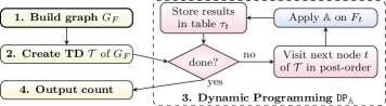
Figure 2: The DP approach, where table algorithm $\mathbb{A}$ modifies tables. [56]

Algorithms that solve Sat or #Sat [31] in linear time for input formulas of bounded treewidth proceed by dynamic programming along the tree decomposition (in post-order) where at each node $t$ of the tree information is gathered [57] in a table $\tau_{t}$. A table $\tau$ is a set of rows, where a row $\vec{}u\in\tau$ is a sequence of fixed length, which is denoted by angle brackets. Tables are derived by an algorithm, which we therefore call table algorithm $\mathbb{A}$. The actual length, content, and meaning of the rows depend on the algorithm $\mathbb{A}$ that derives tables. Therefore, we often explicitly state $\mathbb{A}$-row if rows of this type are syntactically used for table algorithm $\mathbb{A}$ and similar $\mathbb{A}$-table for tables. For sake of comprehension, we specify the rows before presenting the actual table algorithm for manipulating tables. The rows used by a table algorithm $\mathbb{SAT}$ have in common that the first position of these rows manipulated by $\mathbb{SAT}$ consists of an interpretation. The remaining positions of the row depend on the considered table algorithm. For each sequence $\vec{}u\in\tau$, we write $I(\vec{}u)$ to address the interpretation (first) part of the sequence $\vec{}u$. Further, for a given positive integer $i$, we denote by $\vec{}u_{(i)}$ the $i$-th element of row $\vec{}u$ and define $\tau_{(i)}$ as $\tau_{(i)}\,\mathrel{\mathop{:}}=\{\vec{u}_{(i)}\mid\vec{u}\in\tau\}$.

In: Table algorithm $\mathbb{A}$, and instance $(F,P)$ of PMC, a TD $\mathcal{T}=(T,\chi)$ of the primal graph $G_{F}$ of $F$, and tables PP-Tabs.

Out: Table mapping $\mathbb{A}\text{-}\penalty 0\hskip 0.0pt\text{Comp}$, which maps each TD node $t$ of $T$ to some computed table $\tau_{t}$.

1 $\mathbb{A}\text{-}\penalty 0\hskip 0.0pt\text{Comp}\leftarrow\{\}\qquad{\leavevmode\hbox{\set@color{{\hbox{/* }}}}\textnormal{{\ignorespaces empty mapping\hfill */}}}$

2for iterate $t$ in post-order$(T)$ do

3     

4     $\text{Child-Tabs}\leftarrow\langle\mathbb{A}\text{-}\penalty 0\hskip 0.0pt\text{Comp}[t_{1}],\ldots,\mathbb{A}\text{-}\penalty 0\hskip 0.0pt\text{Comp}[t_{\ell}]\rangle$ where $\operatorname{children}(t)=\langle t_{1},\ldots,t_{\ell}\rangle$

5     $\mathbb{A}\text{-}\penalty 0\hskip 0.0pt\text{Comp}[t]\leftarrow{\mathbb{A}}(t,\chi(t),F_{t},P\cap\chi(t),\text{Child-Tabs},{\it{PP}}\hbox{-}\nobreak\hskip 0.0ptTabs)$

return $\mathbb{A}\text{-}\penalty 0\hskip 0.0pt\text{Comp}$

Listing 1 Algorithm ${\mathtt{DP}}_{\mathbb{A}}((F,P),\mathcal{T},{\it{PP}}\hbox{-}\nobreak\hskip 0.0ptTabs)$ for DP on TD ${\cal T}$.

Then, the dynamic programming approach for Boolean satisfiability works as outlined in Figure 2 and performs the following steps:

1. Construct the primal graph $G_{F}$ of $F$.

2. Compute a tree decomposition $(T,\chi)$ of $G_{F}$, obtainable via heuristics.

3. Run $\mathtt{DP}_{\mathbb{SAT}}$, as presented in Listing 1, which executes a table algorithm $\mathbb{SAT}$ for every node $t$ in post-order of the nodes of $T$, and returns $\mathbb{SAT}\text{-}\penalty 0\hskip 0.0pt\text{Comp}$ mapping every node $t$ to its table. $\mathbb{SAT}$ takes as input bag $\chi(t)$, sub-formula $F_{t}$, and tables Child-Tabs previously computed at children of $t$ and outputs a table $\tau_{t}$.

4. Print a positive result whenever the table for node $\operatorname{root}(T)$ is not empty.

The basic steps of the approach are briefly summarized by Listing 2.

In: A Boolean formula $F$ in CNF.

Out: Satisfiability of $F$.

1 $\mathcal{T}=(T,\chi)\leftarrow\text{Decompose\_via\_Heuristics}(G_{F})\qquad{\leavevmode\hbox{\set@color{{\hbox{/* }}}}\textnormal{{\ignorespaces Decompose\hfill */}}}$

2$\mathbb{SAT}\text{-}\penalty 0\hskip 0.0pt\text{Comp}\leftarrow{\mathtt{DP}}_{\mathbb{SAT}}((F,P),\mathcal{T},\emptyset)\qquad{\leavevmode\hbox{\set@color{{\hbox{/* }}}}\textnormal{{\ignorespaces DP via table algorithm $\mathbb{SAT}$\hfill */}}}$

return $\mathbb{PROJ}\text{-}\penalty 0\hskip 0.0pt\text{Comp}[\operatorname{root}(T)]\neq\emptyset$ /* true iff root table is not empty */

Listing 2 Algorithm for solving Sat via dynamic programming.

Listing 3 presents table algorithm $\mathbb{SAT}$ that uses the primal graph representation. We provide only brief intuition, for details we refer to the original source [31]. The main idea is to store in table $\tau_{t}$ only interpretations restricted to bag $\chi(t)$ that can be extended to a model of sub-formula $F_{\leq t}$. Table algorithm $\mathbb{SAT}$ transforms at node $t$ certain row combinations of the tables (Child-Tabs) of child nodes of $t$ into rows of table $\tau_{t}$. The transformation depends on a case where variable $a$ is added or not added to an interpretation (int), removed from an interpretation (rem), or where coinciding interpretations are required (join). In the end, an interpretation $I(\vec{u})$ from a row $\vec{u}$ of the table $\tau_{n}$ at the root $n$ proves that there is a superset $J\supseteq I(\vec{u})$ that is a model of $F=F_{\leq n}$, and hence that the formula is satisfiable.

In: Node $t$, bag $\chi_{t}$, clauses $F_{t}$, and sequence $\text{Child-Tabs}=\langle\tau_{1},\ldots,\tau_{\ell}\rangle$ of child $\mathbb{SAT}$-tables of $t$.

Out: $\mathbb{SAT}$-Table $\tau_{t}.$

1 if $\operatorname{type}(t)=\textit{leaf}$ then $\tau_{t}\leftarrow\{\langle{\color[rgb]{1,0.275,0}\emptyset}\rangle\}$;

2 else if $\operatorname{type}(t)=\textit{int}$ and $a\in\chi_{t}$ is introduced then

3      $\tau_{t}\leftarrow\{\langle{\color[rgb]{1,0.275,0}K}\rangle$ $|\;\langle{\color[rgb]{1,0.275,0}J}\rangle\in\tau_{1},{{{\color[rgb]{0,0,0}K\in\{J,J\cup\{a\}\}},{\color[rgb]{0,0,0}K}}}\vDash F_{t}\}$

4else if $\operatorname{type}(t)=\textit{rem}$ and $a\not\in\chi_{t}$ is removed then

5     $\tau_{t}\leftarrow\{\langle{\color[rgb]{1,0.275,0}J\setminus\{a\}}\rangle$$|\;\langle{\color[rgb]{1,0.275,0}J}\rangle\in\tau_{1}\}$

6 else if $\operatorname{type}(t)=\textit{join}$ then

7     $\tau_{t}\leftarrow\{\langle{\color[rgb]{1,0.275,0}J}\rangle$$|\;\langle{\color[rgb]{1,0.275,0}J}\rangle\in\tau_{1}\cap\tau_{2}\}$

return $\tau_{t}$

Listing 3 Table algorithm $\mathbb{SAT}(t,\chi_{t},F_{t},\cdot,\text{Child-Tabs},\cdot)$ [31].

Example 3 lists selected tables when running algorithm $\mathtt{DP}_{\mathbb{SAT}}$ on a nice tree decomposition. Note that illustration along the lines of a nice TD allows us to visualize the basic cases separately. If one was to implement such an algorithm on general TDs, one still obtains the same basic cases, but interleaved.

Example 3.

Consider formula $F$ from Example 2. Figure 3 illustrates a nice TD $\mathcal{T}^{\prime}=(\cdot,\chi)$ of the primal graph of $F$ and tables $\tau_{1}$, $\ldots$, $\tau_{12}$ that are obtained during the execution of $\mathtt{DP}_{\mathbb{SAT}}((F,\cdot),\mathcal{T}^{\prime},\cdot)$. We assume that each row in a table $\tau_{t}$ is identified by a number, i.e., row $i$ corresponds to $\vec{u_{t.i}}=\langle J_{t.i}\rangle$.

Table $\tau_{1}=\{\langle\emptyset\rangle\}$, due to $\operatorname{type}(t_{1})=\textit{leaf}$. Since $\operatorname{type}(t_{2})=\textit{int}$, we construct table $\tau_{2}$ from $\tau_{1}$ by taking $J_{1.i}$ and $J_{1.i}\cup\{a\}$ for each $\langle J_{1.i}\rangle\in\tau_{1}$. Then, $t_{3}$ introduces $p_{1}$ and $t_{4}$ introduces $b$. $F_{t_{1}}=F_{t_{2}}=F_{t_{3}}=\emptyset$, but since $\chi(t_{4})\subseteq\text{var}(c_{1})$ we have $F_{t_{4}}=\{c_{1},c_{2}\}$ for $t_{4}$. In consequence, for each $J_{4.i}$ of table $\tau_{4}$, we have $\alpha_{{J_{4.i}}}\vDash\{c_{1},c_{2}\}$ since $\mathbb{SAT}$ enforces satisfiability of $F_{t}$ in node $t$. Since $\operatorname{type}(t_{5})=\textit{rem}$, we remove variable $p_{1}$ from all elements in $\tau_{4}$ to construct $\tau_{5}$. Note that we have already seen all rules where $p_{1}$ occurs and hence $p_{1}$ can no longer affect interpretations during the remaining traversal. We similarly create $\tau_{6}=\{\langle\emptyset\rangle,\langle a\rangle\}$ and $\tau_{{10}}=\{\langle a\rangle\}$. Since $\operatorname{type}(t_{11})=\textit{join}$, we build table $\tau_{11}$ by taking the intersection of $\tau_{6}$ and $\tau_{{10}}$. Intuitively, this combines interpretations agreeing on $a$. By definition (primal graph and TDs), for every $c\in F$, variables $\text{var}(c)$ occur together in at least one common bag. Hence, $F=F_{\leq t_{12}}$ and since $\tau_{12}=\{\langle\emptyset\rangle\}$, we can reconstruct for example model $\{a,b,p_{2}\}=J_{11.1}\cup J_{5.4}\cup J_{9.2}$ of $F$ using highlighted (yellow) rows in Figure 3. On the other hand, if $F$ was unsatisfiable, $\tau_{12}$ would be empty ($\emptyset$).

Figure 3: Selected tables obtained by algorithm $\mathtt{DP}_{\mathbb{SAT}}$ on tree decomposition ${\cal T}^{\prime}$.

Interestingly, the above table algorithm $\mathbb{SAT}$ can be easily extended to also count models. Such a table algorithm for solving #Sat works similarly to $\mathbb{SAT}$, but additionally also maintains a counter [31]. There, intuitively, rows of tables for leaf nodes set this counter to $1$ and introduce nodes basically just copy the counter value of child rows. Then, upon removing a certain variable, one has to add (sum up) counters accordingly, and for join nodes counters need to be multiplied. Finally, the counters of the table for the root node can be summed up to obtain the solution to the #Sat problem.

3.2 (Re-)constructing Interpretations and Models

Even further, with the help of the obtained tables during dynamic programming, one can actually construct (projected) models by combining suitable predecessor rows. The idea is to combine those obtained rows that contain parts of models that fit together. To this end, we require the following definition, which we will also use later. At a node $t$ and for a row $\vec{}u$ of the computed table $\mathbb{SAT}\text{-}\penalty 0\hskip 0.0pt\text{Comp}[t]$, it yields the originating rows in the tables of the children of $t$ that were involved in computing row $\vec{}u$ by algorithm $\mathbb{SAT}$.

Definition 1 (Origins, cf., [41]).

Let $F$ be a formula, $\mathcal{T}=(T,\chi)$ be a tree decomposition of $F$, $t$ be a node of $T$ with $\operatorname{children}(t)=\langle t_{1},\ldots,t_{\ell}\rangle$, and $\tau_{1}\in\mathbb{SAT}\text{-}\penalty 0\hskip 0.0pt\text{Comp[$t_{1}$]},\ldots,\tau_{\ell}\in\mathbb{SAT}\text{-}\penalty 0\hskip 0.0pt\text{Comp[$t_{\ell}$]}$ be the tables computed by $\mathtt{DP}_{\mathbb{SAT}}$.

For a given $\mathbb{SAT}$-row $\vec{u}$ in $\mathbb{SAT}\text{-}\penalty 0\hskip 0.0pt\text{Comp[$t$]}$, we define its originating $\mathbb{SAT}$-rows by $\operatorname{Origins}(t,\vec{}u){\,\mathrel{\mathop{:}}=}\{\vec{s}\mid\vec{s}\in\tau_{1}\times\cdots\times\tau_{\ell},\tau={\mathbb{SAT}}(t,\chi(t),F_{t},\cdot,\langle\{\vec{s}\}\rangle,\cdot),\vec{u}\in\tau\}.$ We naturally extend this to a $\mathbb{SAT}$-table $\sigma$ by $\operatorname{Origins}(t,\sigma){\,\mathrel{\mathop{:}}=}$ $\bigcup_{\vec{u}\in\sigma}\operatorname{Origins}(t,\vec{u}).$

Example 4 illustrates Definition 1 for our running example, where we briefly show origins for some rows of selected tables.

Example 4.

Consider formula $F$, tree decomposition $\mathcal{T}^{\prime}=(T,\chi)$, and tables $\tau_{1},\ldots,\tau_{12}$ from Example 3. We focus on $\vec{u_{1.1}}=\langle J_{1.1}\rangle=\langle\emptyset\rangle$ of table $\tau_{1}$ of the leaf $t_{1}$. The row $\vec{u_{1.1}}$ has no preceding row, since $\operatorname{type}(t_{1})=\textit{leaf}$. Hence, we have $\operatorname{Origins}(t_{1},\vec{u_{1.1}})=\{\langle\rangle\}$. The origins of row $\vec{u_{5.1}}$ of table $\tau_{5}$ are given by $\operatorname{Origins}(t_{5},\vec{u_{5.1}})$, which correspond to the preceding rows in table $t_{4}$ that lead to row $\vec{u_{5.1}}$ of table $\tau_{5}$ when running algorithm $\mathbb{SAT}$, i.e., $\operatorname{Origins}(t_{5},\vec{u_{5.1}})=\{\langle\vec{u_{4.1}}\rangle,\langle\vec{u_{4.4}}\rangle\}$. Observe that $\operatorname{Origins}(t_{i},\vec{}u)=\emptyset$ for any row $\vec{}u\not\in\tau_{i}$. For node $t_{11}$ of type join and row $\vec{u_{11.1}}$, we obtain $\operatorname{Origins}(t_{11},\vec{u_{11.1}})=\{\langle\vec{u_{6.2}},$ $\vec{u_{10.1}}\rangle\}$ (see Example 3). More general, when using algorithm $\mathbb{SAT}$, at a node $t$ of type join with table $\tau$ we have $\operatorname{Origins}(t,\vec{u})=\{\langle\vec{}u,\vec{}u\rangle\}$ for row $\vec{u}\in\tau$.

Definition 1 refers to the predecessors of rows. In order to reconstruct models, one needs to recursively combine these origins from a node $t$ down to the leafs. This idea of combining suitable rows is formalized in the following definition, which introduces the concept of extensions. Thereby, rows are extended such that one can then reconstruct models from these extensions.

Definition 2 (Extensions).

Let $F$ be a formula, $\mathcal{T}=(T,\chi)$ be a tree decomposition, $t$ be a node of $T$, and $\vec{u}$ be a row of $\mathbb{SAT}\text{-}\penalty 0\hskip 0.0pt\text{Comp}[t]$.

An extension below $t$ is a set of pairs where a pair consists of a node $t^{\prime}$ of $T[t]$ and a row $\vec{v}$ of $\mathbb{SAT}\text{-}\penalty 0\hskip 0.0pt\text{Comp}[t^{\prime}]$ and the cardinality of the set equals the number of nodes in the sub-tree $T[t]$. We define the family of extensions below $t$ recursively as follows. If $t$ is of type leaf, then $\operatorname{Exts}_{\leq t}(\vec{u}){\,\mathrel{\mathop{:}}=}\{\{\langle t,\vec{u}\rangle\}\}$; otherwise $\operatorname{Exts}_{\leq t}(\vec{u}){\,\mathrel{\mathop{:}}=}\bigcup_{\vec{v}\in\operatorname{Origins}(t,\vec{u})}\big{\{}\{\langle t,\vec{u}\rangle\}\cup X_{1}\cup\ldots\cup X_{\ell}\mid X_{i}\in\operatorname{Exts}_{\leq t_{i}}({\vec{v}}_{(i)})\big{\}}$ for the $\ell$ children $t_{1},\ldots,t_{\ell}$ of $t$. We lift this notation for a $\mathbb{SAT}$-table $\sigma$ by $\operatorname{Exts}_{\leq t}(\sigma){\,\mathrel{\mathop{:}}=}\bigcup_{\vec{u}\in\sigma}\operatorname{Exts}_{\leq t}(\vec{u})$. Further, we let $\operatorname{Exts}{\,\mathrel{\mathop{:}}=}\operatorname{Exts}_{\leq n}(\mathbb{SAT}\text{-}\penalty 0\hskip 0.0pt\text{Comp}[n])$.

Indeed, if we construct extensions below the root $n$, it allows us to also obtain all models of a formula $F$. Finally, we define notation that gives us a way to reconstruct interpretations from such (families of) extensions.

Definition 3 (Interpretations of Extensions).

Let $(F,P)$ be an instance of PMC, $\mathcal{T}=(T,\chi)$ be a tree decomposition of $F$, $t$ be a node of $T$. Further, let $E$ be a family of extensions below $t$, and $P$ be a set of projection variables. We define the set $I(E)$ of interpretations of $E$ by $I(E){\,\mathrel{\mathop{:}}=}\big{\{}\bigcup_{\langle\cdot,\vec{u}\rangle\in X}I(\vec{u})\mid X\in E\big{\}}$ and the set $I_{P}(E)$ of projected interpretations by $I_{P}(E){\,\mathrel{\mathop{:}}=}\big{\{}\bigcup_{\langle\cdot,\vec{u}\rangle\in X}I(\vec{u})\cap P\mid X\in E\big{\}}$.

We briefly illustrate these concepts along the lines of our running example.

Example 5.

Consider again formula $F$ and tree decomposition ${\cal T}^{\prime}$ with root $n$ of $F$ from Example 3. Let $X=\{\langle t_{12},\langle\emptyset\rangle\rangle,\langle t_{11},\langle\{a\}\rangle\rangle,$ $\langle t_{6},\langle\{a\}\rangle\rangle,\langle t_{5},\langle\{a,b\}\rangle\rangle,$ $\langle t_{4},\langle\{a,b\}\rangle\rangle,$ $\langle t_{3},\langle\{a\}\rangle\rangle,\langle t_{2},\langle\{a\}\rangle\rangle,\langle t_{1},\langle\emptyset\rangle\rangle,\langle t_{10},\langle\{a\}\rangle\rangle,\langle t_{9},$ $\langle\{a,p_{2}\}\rangle\rangle,\langle t_{8},\langle\{p_{2}\}\rangle\rangle,$ $\langle t_{7},\langle\emptyset\rangle\rangle\}$ be an extension below $n$. Observe that $X\in\operatorname{Exts}$ and that Figure 3 highlights those rows of tables for nodes $t_{12},t_{11},t_{9},t_{5},t_{4}$ and $t_{1}$ that also occur in $X$ (in yellow). Further, $I(\{X\})=\{a,b,p_{2}\}$ computes the corresponding model of $X$, and $I_{P}(\{X\})=\{p_{2}\}$ derives the projected model of $X$. $I(\operatorname{Exts})$ refers to the set of models of $F$, whereas $I_{P}(\operatorname{Exts})$ is the set of projected models of $F$.

In order to only construct extensions that correspond to (parts of) models of the formula, we simply need to access only those extensions that contain rows that lead to models of the formula. As already observed in the previous example, these rows are precisely the ones contained in $\operatorname{Exts}$. The resulting extensions for a node $t$ are formalized in the following concept of satisfiable extensions, whereby we take only those extensions of $\operatorname{Exts}_{\leq t}$ that are also contained in $\operatorname{Exts}$.

Definition 4 (Satisfiable Extension).

Let $F$ be a formula, $\mathcal{T}=(T,\chi)$ be a tree decomposition of $F$, $t$ be a node of $T$, and $\sigma\subseteq\mathbb{SAT}\text{-}\penalty 0\hskip 0.0pt\text{Comp}[t]$ be a set of rows. Then, we define the satisfiable extensions below $t$ for $\sigma$ by $\operatorname{SatExt}_{\leq t}(\sigma){\,\mathrel{\mathop{:}}=}\bigcup_{\vec{u}\in\sigma}\{X\mid X\in\operatorname{Exts}_{\leq t}(\vec{u}),X\subseteq Y,Y\in\operatorname{Exts}\}.$

4 Counting Projected Models by Dynamic Programming

While the transition from deciding Sat to solving #Sat is quite simple by adding an additional counter, it turns out that the problem PMC requires more effort. We solve this problem PMC by providing an algorithm in Section 4.1 that utilizes treewidth and adheres to multiple passes (rounds) of computation that are guided along a tree decomposition. Then, we give detailed formal arguments on correctness of this algorithm in Section 4.2. Later, in Section 4.3 we discuss complexity results in the form of matching upper and lower bounds, where it turns out that our algorithm cannot be significantly improved.

4.1 Solving PMC by means of Dynamic Programming

Next, we introduce the dynamic programming algorithm $\mathtt{PCNT}_{\mathbb{SAT}}$ to solve the projected model counting problem (PMC) for Boolean formulas. From a high-level perspective, our algorithm builds upon the table algorithm $\mathbb{SAT}$ from the previous section; we assume again a formula $F$ and a tree decomposition $\mathcal{T}=(T,\chi)$ of $F$, and additionally a set $P$ of projection variables. Thereby, the table for each tree decomposition node $t$ consists of a set $\sigma$ of assignments restricted to bag variables $\chi(t)$ (as computed by $\mathbb{SAT}$) that agree on their assignment of variables in $P\cap\chi(t)$, and a counter $c$. Intuitively, this counter $c$ counts those satisfying assignments of $F_{\leq t}$ restricted to $P\cap\chi(t)$ that are among satisfiable extensions and extend any assignment in $\sigma$. Then, for the (empty) tree decomposition root $n$, there is only one single counter which is the projected model count of $F$ with respect to $P$. The challenge of our algorithm $\mathtt{PCNT}_{\mathbb{SAT}}$ is to compute these counts $c$ by only considering local information, i.e., previously computed tables of child nodes of $t$. To this end, we utilize mathematical combinatorics, namely the principle of inclusion-exclusion principle [46], which we need to apply in an interleaved fashion.

Concretely, our algorithm $\mathtt{PCNT}_{\mathbb{SAT}}$ traverses the tree decomposition twice following a multi-pass dynamic programming paradigm [41]. Figure 4 illustrates the steps of our algorithm $\mathtt{PCNT}_{\mathbb{SAT}}$, which are also presented in the form of Listing 4. Similar to the previous section (cf., Figure 2), we construct a graph representation and heuristically compute a tree decomposition of this graph. Then, we run $\mathtt{DP}_{\mathbb{SAT}}$ (see Listing 1) in Step 3a as first pass. Step 3a can also be seen as a preprocessing step for projected model counting, from which we immediately know whether the formula has a model. However, we keep the $\mathbb{SAT}$-tables that have been computed in Step 3a. These tables form the basis for the next step.

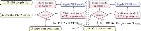
Figure 4: Algorithm $\mathtt{PCNT}_{\mathbb{SAT}}$ consists of $\mathtt{DP}_{\mathbb{SAT}}$ and $\mathtt{DP}_{\mathbb{PROJ}}$.

In: An instance $(F,P)$ of PMC.

Out: The projected model count of $(F,P)$.

1 $\mathcal{T}=(T,\chi)\leftarrow\text{Decompose\_via\_Heuristics}(G_{F})\qquad{\leavevmode\hbox{\set@color{{\hbox{/* }}}}\textnormal{{\ignorespaces Decompose\hfill */}}}$

2$\mathbb{SAT}\text{-}\penalty 0\hskip 0.0pt\text{Comp}\leftarrow{\mathtt{DP}}_{\mathbb{SAT}}((F,P),\mathcal{T},\emptyset)\qquad{\leavevmode\hbox{\set@color{{\hbox{/* }}}}\textnormal{{\ignorespaces DP via table algorithm $\mathbb{SAT}$\hfill */}}}$

3/* Purge non-solutions of $\mathbb{SAT}\text{-}\penalty 0\hskip 0.0pt\text{Comp}$; ensured by using $\operatorname{SatExt}$ below. */

4$\mathbb{PROJ}\text{-}\penalty 0\hskip 0.0pt\text{Comp}\leftarrow{\mathtt{DP}}_{\mathbb{PROJ}}((F,P),\mathcal{T},\mathbb{SAT}\text{-}\penalty 0\hskip 0.0pt\text{Comp})\quad{\leavevmode\hbox{\set@color{{\hbox{/* }}}}\textnormal{{\ignorespaces DP via algorithm $\mathbb{PROJ}$\hfill */}}}$

return $\sum_{\langle\varphi,c\rangle\in\mathbb{PROJ}\text{-}\penalty 0\hskip 0.0pt\text{Comp}[\operatorname{root}(T)]}c$  /* Return projected model count */

Listing 4 Algorithm $\mathtt{PCNT}_{\mathbb{SAT}}(F,P)$ for solving PMC via dynamic programming.

There, we remove all rows from the obtained $\mathbb{SAT}$-tables which cannot be extended to a model of the Sat problem (“Purge non-solutions”). In other words, we keep only rows $\vec{u}$ in table $\mathbb{SAT}\text{-}\penalty 0\hskip 0.0pt\text{Comp}[t]$ at node $t$ if its interpretation $I(\vec{u})$ can be extended to a model of $F$. Thereby, we avoid redundancies and can simplify the description and presentation of our next step, since we then only consider rows that are (parts of) models. Intuitively, the rows involving non-models contributes only non-relevant information, as also observed in related works [37, 58]. Formally, this is achieved by utilizing satisfiable extensions as defined in Definition 4, since these extensions precisely consider the rows that contribute to models.

In Step 3b ($\mathtt{DP}_{\mathbb{PROJ}}$), we perform the second pass, where we traverse the tree decomposition a second time to count projections of interpretations of rows in $\mathbb{SAT}$-tables. Observe that the tree traversal in $\mathtt{DP}_{\mathbb{PROJ}}$ is the same as before. Therefore, in the following, we describe the ingredients that lead to table algorithm $\mathbb{PROJ}$. For $\mathbb{PROJ}$, a row at a node $t$ is a pair $\langle\sigma,c\rangle$ where $\sigma$ is a $\mathbb{SAT}$-table, in particular, a subset of $\mathbb{SAT}\text{-}\penalty 0\hskip 0.0pt\text{Comp}[t]$ computed by $\mathtt{DP}_{\mathbb{SAT}}$, and $c$ is a non-negative integer. Below, we characterize $\sigma$, which is based on grouping rows in equivalence classes.

Equivalence Classes for $\mathbb{SAT}$-Tables. The following definitions provide central notions for grouping rows of tables according to the given projection of variables, which yields an equivalence relation.

Definition 5.

Let $(F,P)$ be an instance of PMC and $\sigma$ be a $\mathbb{SAT}$-table. We define the relation $\operatorname{=_{P}}\subseteq\sigma\times\sigma$ to consider equivalent rows with respect to the projection of its interpretations by $\operatorname{=_{P}}{\,\mathrel{\mathop{:}}=}\{(\vec{u},\vec{v})\mid\vec{u},\vec{v}\in\sigma,I(\vec{u})\cap P=I(\vec{v})\cap P\}.$

Observation 1.

The relation $\operatorname{=_{P}}$ is an equivalence relation.

Based on this equivalence relation, we define corresponding equivalence classes.

Definition 6 (Equivalence Classes).

Let $\tau$ be a $\mathbb{SAT}$-table and $\vec{u}$ be a row of $\tau$. The relation $\operatorname{=_{P}}$ induces equivalence classes $[\vec{u}]_{P}$ on the $\mathbb{SAT}$-table $\tau$ in the usual way, i.e., $[\vec{u}]_{P}=\{\vec{v}\mid\vec{v}\operatorname{=_{P}}\vec{u},\vec{v}\in\tau\}$ [59]. We denote by $\operatorname{EqClasses}_{P}(\tau)$ the set of equivalence classes of $\tau$, i.e., $\operatorname{EqClasses}_{P}(\tau){\,\mathrel{\mathop{:}}=}\,(\tau/\operatorname{=_{P}})=\{[\vec{u}]_{P}\mid\vec{u}\in\tau\}$.

These classes are briefly demonstrated on our running example.

Example 6.

Consider again formula $F$ and set $P$ of projection variables from Example 1 and tree decomposition $\mathcal{T}^{\prime}=(T,\chi)$ and $\mathbb{SAT}$-table $\tau_{4}$ from Figure 3. We have $\vec{u_{4.1}}=_{P}\vec{u_{4.2}}$ and $\vec{u_{4.4}}=_{P}\vec{u_{4.5}}$. We obtain the set $\tau_{4}/\operatorname{=_{P}}$ of equivalence classes of $\tau_{4}$ by $\operatorname{EqClasses}_{P}(\tau_{4})=\{\{\vec{u_{4.1}},\vec{u_{4.2}},\vec{u_{4.3}}\},\{\vec{u_{4.4}},$ $\vec{u_{4.5}},\vec{u_{4.6}}\}\}$.

Indeed, the algorithm $\mathbb{PROJ}$, stores at a node $t$ pairs $\langle\sigma,c\rangle$, where $\sigma$ is actually a (non-empty) subset of the equivalence classes in $\operatorname{EqClasses}_{P}(\mathbb{SAT}\text{-}\penalty 0\hskip 0.0pt\text{Comp}[t])$. Next, we discuss how the integer $c$ aids in projected counting for such a subset $\sigma$.

Counting for Equivalence Classes. In fact, we store in integer $c$ a count that expresses the number of “intersection” projected models ($\operatorname{ipmc}$) that indicates for $\sigma$ the number of projected models up to node $t$ that the rows in $\sigma$ haves in common (intersection of models). In the end, we aim for the projected model count ($\operatorname{pmc}$), i.e., the combined number of projected models (union of models), where $\sigma$ is involved. However, it turns out that the process of computing these projected model counts will be heavily interleaved with the $\operatorname{ipmc}$ counts. In the following, we define both counts for a node $t$ of a tree decomposition by means of the satisfying extensions below $t$.

Notably, the effort of directly computing these counts when strictly following the definition below would not result in an algorithm that is fixed-parameter tractable. As a result, our approach is then subsequently developed thereafter, without explicitly involving every descendant node below $t$ in order to fulfill the desired runtime claims.

Definition 7.

Let $(F,P)$ be an instance of PMC, $\mathcal{T}=(T,\chi)$ be a tree decomposition of $F$, $t$ be a node of $T$, and $\sigma\subseteq\mathbb{SAT}\text{-}\penalty 0\hskip 0.0pt\text{Comp}[t]$ be a set of $\mathbb{SAT}$-rows for node $t$. Then, the intersection projected model count $\operatorname{ipmc}_{\leq t}(\sigma)$ of $\sigma$ below $t$ is the size of the intersection over projected interpretations of the satisfiable extensions of $\sigma$ below $t$, i.e., $\operatorname{ipmc}_{\leq t}(\sigma){\,\mathrel{\mathop{:}}=}|\bigcap_{\vec{u}\in\sigma}I_{P}(\operatorname{SatExt}_{\leq t}(\{\vec{u}\}))|$.

The projected model count $\operatorname{pmc}_{\leq t}(\sigma)$ of $\sigma$ below $t$ is the size of the union over projected interpretations of the satisfiable extensions of $\sigma$ below $t$, formally, $\operatorname{pmc}_{\leq t}(\sigma){\,\mathrel{\mathop{:}}=}|\bigcup_{\vec{u}\in\sigma}I_{P}(\operatorname{SatExt}_{\leq t}(\{\vec{u}\}))|$.

Note that this definition relies on satisfiable extensions as given in Definition 4. Intuitively, the counts $\operatorname{ipmc}_{\leq t}$ represent for a set $\sigma$ of $\mathbb{SAT}$-rows, the cardinality of those projected models of $F_{\leq t}$ that can be extended to models of $F$, where every row in $\sigma$ is involved. Consequently, for the root $n$ of a nice tree decomposition of $F$ we have that $\operatorname{ipmc}_{\leq n}(\{\langle\emptyset\rangle\})=\operatorname{pmc}_{\leq n}(\{\langle\emptyset\rangle\})$ coincides with the projected model count of $F$. This is the case since $F_{\leq n}=F$, the bag of $n$ is empty, and therefore the $\mathbb{SAT}$-table for $n$ contains one row if and only if $F$ is satisfiable.

Observe that when computing these counts for a node $t$, we cannot directly count models since this would not yield a fixed-parameter tractability algorithm. Instead, in order to count, we may only utilize counters for sets $\sigma$ of rows in tables of $t$ and direct child nodes of $t$, which is more involved than directly counting models. This is established for $\operatorname{pmc}$ next by relying on combinatorial counting principles like inclusion-exclusion [46].

Computing Projected Model Counts ($\operatorname{pmc}$). Since $\mathbb{PROJ}$ stores in $\mathbb{PROJ}$-tables an $\mathbb{SAT}$-table together with a counter, in the end we need to describe how these counters are maintained. As the first step, we show how for a node $t$, these counters ($\operatorname{ipmc}$ values) for child tables of $t$ can be used to compute $\operatorname{pmc}$ values for $t$. Intuitively, when we are at a node $t$ in the Algorithm $\mathtt{DP}_{\mathbb{PROJ}}$ we already computed all tables $\mathbb{SAT}\text{-}\penalty 0\hskip 0.0pt\text{Comp}$ by $\mathtt{DP}_{\mathbb{SAT}}$ according to Step 3a, purged non-solutions, and computed $\mathbb{PROJ}\text{-}\penalty 0\hskip 0.0pt\text{Comp}[t^{\prime}]$ for all nodes $t^{\prime}$ below $t$ and in particular the $\mathbb{PROJ}$-tables Child-Tabs of the children of $t$. Then, we compute the projected model count of a subset $\sigma$ of the $\mathbb{SAT}$-rows in $\mathbb{SAT}\text{-}\penalty 0\hskip 0.0pt\text{Comp}[t]$, which we formalize by applying the generalized inclusion-exclusion principle to the stored intersection projected model counts of origins.

The idea behind the following definition is that for every origin of $\sigma$, we lift the $\operatorname{ipmc}$ counts that are stored in the corresponding child tables. However, if we sum up these counts, those models that two origins have in common are over-counted, i.e., they need to be subtracted. But then, those models that three origins have in common are under-counted, i.e., they need to be (re-)added again. In turn, the inclusion-exclusion principle ensures that we obtain the correct $\operatorname{pmc}$ value for $\sigma$.

Definition 8.

Let $(F,P)$ be an instance of PMC, $\mathcal{T}=(T,\chi)$ be a tree decomposition of $F$, and $t$ be a node of $T$ with $\ell$ children. Further, let $\text{Child-Tabs}=\langle\mathbb{PROJ}\text{-}\penalty 0\hskip 0.0pt\text{Comp}[t_{1}],\ldots,\mathbb{PROJ}\text{-}\penalty 0\hskip 0.0pt\text{Comp}[t_{\ell}]\rangle$ be the sequence of $\mathbb{PROJ}$-tables computed by $\mathtt{DP}_{\mathbb{PROJ}}((F,P),\mathcal{T},\mathbb{SAT}\text{-}\penalty 0\hskip 0.0pt\text{Comp})$, where $\operatorname{children}(t)=\langle t_{1},\ldots,t_{\ell}\rangle$ and $\sigma\subseteq\mathbb{SAT}\text{-}\penalty 0\hskip 0.0pt\text{Comp}[t]$ is a table. We define the (inductive) projected model count of $\sigma$:

$$\operatorname{pmc}(t,\sigma,\text{Child-Tabs}){\,\mathrel{\mathop{:}}=} \sum_{\emptyset\subsetneq O\subseteq{\operatorname{Origins}(t,\sigma)}}(-1)^{(|O|-1)}\cdot\operatorname{s-ipmc}(\text{Child-Tabs},O),\text{where}$$

$$\operatorname{s-ipmc}(\text{Child-Tabs},O){\,\mathrel{\mathop{:}}=} \prod_{\begin{subarray}{c}i\in\{1,\ldots,\ell\},\\ \langle O_{(i)},c\rangle\in\mathbb{PROJ}\text{-}\penalty 0\hskip 0.0pt\text{Comp}[t_{i}]\end{subarray}}c\quad\text{is the \emph{stored ipmc} from child tables}.$$

Vaguely speaking, $\operatorname{pmc}$ determines the origins of the set $\sigma$ of rows, goes over all subsets of these origins and looks up the stored counts ($\operatorname{s-ipmc}$) in the $\mathbb{PROJ}$-tables of the children of $t$. There, we may simply have several child nodes, i.e., nodes of type join, and hence in this case we need to multiply the corresponding children’s (independent) $\operatorname{ipmc}$ values.

Example 7 provides an idea on how to compute the projected model count of tables of our running example using $\operatorname{pmc}$.

Example 7.

The function defined in Definition 8 allows us to compute the projected count for a given $\mathbb{SAT}$-table. Therefore, consider again formula $F$ and tree decomposition $\mathcal{T}^{\prime}$ from Example 2 and Figure 3. Say we want to compute the projected count $\operatorname{pmc}(t_{5},\{\vec{u_{5.4}}\},\text{Child-Tabs})$ where $\text{Child-Tabs}{\,\mathrel{\mathop{:}}=}\allowdisplaybreaks[4]\big{\{}\langle\{\vec{u_{4.3}}\},1\rangle,$ $\langle\{\vec{u_{4.6}}\},1\rangle\big{\}}$ for row $\vec{u_{5.4}}$ of table $\tau_{5}$. Note that $t_{5}$ has $\ell=1$ child nodes $\langle t_{4}\rangle$ and therefore the product of Definition 8 consists of only one factor. Observe that $\operatorname{Origins}(t_{5},\vec{u_{5.4}})=\{\langle\vec{u_{4.3}}\rangle,\langle\vec{u_{4.6}}\rangle\}$. Since the rows $\vec{u_{4.3}}$ and $\vec{u_{4.6}}$ do not occur in the same $\mathbb{SAT}$-table of Child-Tabs, only the value of $\operatorname{s-ipmc}$ for the two singleton origin sets $\{\langle\vec{u_{4.3}}\rangle\}$ and $\{\langle\vec{u_{4.6}}\rangle\}$ is non-zero; for the remaining set of origins we have zero. Hence, we obtain $\operatorname{pmc}(t_{5},\{\vec{u_{5.4}}\},\text{Child-Tabs})=2$.

Computing Intersection Projected Model Counts ($\operatorname{ipmc}$). Before we present algorithm $\mathbb{PROJ}$ (Listing 5), we give the the definition allowing us at a certain node $t$ to obtain the $\operatorname{ipmc}$ value for a given $\mathbb{SAT}$-table $\sigma$ by computing the $\operatorname{pmc}$ (using stored $\operatorname{ipmc}$ values from $\mathbb{PROJ}$-tables for children of $t$), and subtracting and adding $\operatorname{ipmc}$ values for subsets $\emptyset\subsetneq\rho\subsetneq\sigma$ accordingly.

The intuition is that in order to obtain the number of those common projected models, where every single row in $\sigma$ participates, we take all involved projected models of $\sigma$ and subtract every single row’s projected model count ($\operatorname{ipmc}$ values). There, we subtracted those models that two rows have in common more than once. Again, these models need to be re-added. Then, the models that three rows have in common are subtracted and so forth. In turn, we end up with the intersection projected model count, i.e., those projected models, where every row of $\sigma$ is involved.

Definition 9.

Let $\mathcal{T}=(T,\chi)$ be a tree decomposition, $t$ be a node of $T$, $\sigma$ be a $\mathbb{SAT}$-table, and Child-Tabs be a sequence of tables. Then, we define the (recursive) $\operatorname{ipmc}$ of $\sigma$ as follows:

$$\operatorname{ipmc}(t,\sigma,\text{Child-Tabs}){\,\mathrel{\mathop{:}}=}\begin{cases}1,\text{ if }\operatorname{type}(t)=\textit{leaf},\\ \big{|}\operatorname{pmc}(t,\sigma,\text{Child-Tabs})\;+\\ \quad\sum_{\emptyset\subsetneq\rho\subsetneq\sigma}(-1)^{|\rho|}\cdot\operatorname{ipmc}(t,\rho,\text{Child-Tabs})\big{|},\text{otherwise.}\end{cases}$$

In other words, if a node is of type leaf the $\operatorname{ipmc}$ is one, since by definition of a tree decomposition the bags of nodes of type leaf contain only one projected interpretation (the empty set). Otherwise, using Definition 8, we are able to compute the $\operatorname{ipmc}$ for a given $\mathbb{SAT}$-table $\sigma$, which is by construction the same as $\operatorname{ipmc}_{\leq t}(\sigma)$ (cf., proof of Theorem 1 later). In more detail, we want to compute for a $\mathbb{SAT}$-table $\sigma$ its $\operatorname{ipmc}$ that represents “all-overlapping” counts of $\sigma$ with respect to set $P$ of projection variables, that is, $\operatorname{ipmc}_{\leq t}(\sigma)$. Therefore, for $\operatorname{ipmc}$, we rearrange the inclusion-exclusion principle. To this end, we take $\operatorname{pmc}$, which computes the “non-overlapping” count of $\sigma$ with respect to $P$, by once more exploiting the inclusion-exclusion principle on origins of $\sigma$ (as already discussed) such that we count every projected model only once. Then we have to alternately subtract and add $\operatorname{ipmc}$ values for strict subsets $\rho$ of $\sigma$, accordingly.

We provide an example on how this definition is carried out below.

The Table Algorithm $\mathbb{PROJ}$. Finally, Listing 5 presents table algorithm $\mathbb{PROJ}$, which stores for given node $t$ a $\mathbb{PROJ}$-table consisting of every non-empty subset of equivalence classes for the given table $\mathbb{SAT}\text{-}\penalty 0\hskip 0.0pt\text{Comp[$t$]}$ together with its $\operatorname{ipmc}$ (as presented above).

In: Node $t$, set $P$ of projection variables, Child-Tabs, and $\mathbb{SAT}\text{-}\penalty 0\hskip 0.0pt\text{Comp}$.

Out: Table $\iota_{t}$ consisting of pairs $\langle\sigma,c\rangle$, where $\sigma\subseteq\mathbb{SAT}\text{-}\penalty 0\hskip 0.0pt\text{Comp[$t$]}$ and $c\in\mathbb{N}$.

1 $\makebox[0.0pt]{}\iota_{t}\leftarrow\big{\{}\langle\sigma,\operatorname{ipmc}(t,\sigma,\text{Child-Tabs})\rangle\big{|}\,C\in\operatorname{EqClasses}_{P}(\mathbb{SAT}\text{-}\penalty 0\hskip 0.0pt\text{Comp[$t$]}),\emptyset\subsetneq\sigma\subseteq C\big{\}}$ ;

return $\iota_{t}$

Listing 5 Table algorithm $\mathbb{PROJ}(t,\cdot,\cdot,P,\text{Child-Tabs},\mathbb{SAT}\text{-}\penalty 0\hskip 0.0pt\text{Comp})$.

Example 8.

Recall instance $(F,P)$ of PMC, tree decomposition $\mathcal{T}^{\prime}$, and tables $\tau_{1}$, $\ldots$, $\tau_{12}$ from Example 1, 3, and Figure 3. Figure 5 depicts selected tables of $\iota_{1},\ldots\iota_{12}$ obtained after running $\mathtt{DP}_{\mathbb{PROJ}}$ for counting projected interpretations. We assume numbered rows, i.e., row $i$ in table $\iota_{t}$ corresponds to $\vec{v_{t.i}}=\langle\sigma_{t.i},c_{t.i}\rangle$. Note that for some nodes $t$, there are rows among different $\mathbb{SAT}$-tables that occur in $\operatorname{Exts}_{\leq t}$, but not in $\operatorname{SatExt}_{\leq t}$. These rows are removed during purging. In fact, rows $\vec{u_{4.1}},\vec{u_{4.2}}$, and $\vec{u_{4.4}}$ do not occur in table $\iota_{4}$. Observe that purging is a crucial trick here that avoids to correct stored counters $c$ by backtracking whenever a certain row of a table has no succeeding row in the parent table.

Next, we discuss selected rows obtained by $\mathtt{DP}_{\mathbb{PROJ}}((F,P),\mathcal{T}^{\prime},\mathbb{SAT}\text{-}\penalty 0\hskip 0.0pt\text{Comp})$. Tables $\iota_{1}$, $\ldots$, $\iota_{12}$ that are computed at the respective nodes of the tree decomposition are shown in Figure 5. Since $\operatorname{type}(t_{1})=\textit{leaf}$, we have $\iota_{1}=\langle\{\langle\emptyset\rangle\},1\rangle$. Intuitively, up to node $t_{1}$ the $\mathbb{SAT}$-row $\langle\emptyset\rangle$ belongs to $1$ equivalence class. Node $t_{2}$ introduces variable $a$, which results in table $\iota_{2}{\,\mathrel{\mathop{:}}=}\big{\{}\langle\{\langle\{a\}\rangle\},1\rangle\big{\}}$. Note that the $\mathbb{SAT}$-row $\langle\emptyset\rangle$ is subject to purging. Node $t_{3}$ introduces $p_{1}$ and node $t_{4}$ introduces $b$. Node $t_{5}$ removes projection variable $p_{1}$. The row $\vec{v_{5.2}}$ of $\mathbb{PROJ}$-table $\iota_{5}$ has already been discussed in Example 7 and row $\vec{v_{5.1}}$ works similar. For row $\vec{v_{5.3}}$ we compute the count $\operatorname{ipmc}(t_{5},\{\vec{u_{5.2}},\vec{u_{5.4}}\},\langle\iota_{4}\rangle)$ by means of $\operatorname{pmc}$. Therefore, take for $\rho$ the sets $\{\vec{u_{5.2}}\}$, $\{\vec{u_{5.4}}\}$, and $\{\vec{u_{5.2}},\vec{u_{5.4}}\}$. For the singleton sets, we simply have $\operatorname{pmc}(t_{5},\{\vec{u_{5.2}}\},\langle\iota_{4}\rangle)=\operatorname{ipmc}(t_{5},\{\vec{u_{5.2}}\},\langle\iota_{4}\rangle)=c_{5.1}=1$ and $\operatorname{pmc}(t_{5},\{\vec{u_{5.4}}\},\langle\iota_{4}\rangle)=\operatorname{ipmc}(t_{5},\{\vec{u_{5.4}}\},\langle\iota_{4}\rangle)=c_{5.2}=2$. To compute $\operatorname{pmc}(t_{5},\{\vec{u_{5.2}},\vec{u_{5.4}}\},\langle\iota_{4}\rangle)$ following Definition 8, take for $O$ the sets $\{\vec{u_{4.5}}\}$, $\{\vec{u_{4.3}}\}$, and $\{\vec{u_{4.6}}\}$ into account, since all other non-empty subsets of origins of $\vec{u_{5.2}}$ and $\vec{u_{5.4}}$ in $\iota_{4}$ do not occur in $\iota_{4}$. Then, we take the sum over the values $\operatorname{s-ipmc}(\langle\iota_{4}\rangle,\{\langle\vec{u_{4.5}}\rangle\})=1$, $\operatorname{s-ipmc}(\langle\iota_{4}\rangle,\{\langle\vec{u_{4.3}}\rangle\})=1$, and $\operatorname{s-ipmc}(\langle\iota_{4}\rangle,\{\langle\vec{u_{4.6}}\rangle\})$ $=1$; and subtract $\operatorname{s-ipmc}(\langle\iota_{4}\rangle,$ $\{\langle\vec{u_{4.5}}\rangle,\langle\vec{u_{4.6}}\rangle\})=1$. Hence, $\operatorname{pmc}(t_{5},\{\vec{u_{5.2}},\vec{u_{5.4}}\},$ $\langle\iota_{4}\rangle)=2$. In order to compute $\operatorname{ipmc}(t_{5},\{\vec{u_{5.2}},\vec{u_{5.4}}\},\langle\iota_{4}\rangle)=|\operatorname{pmc}(t_{5},\{\vec{u_{5.2}},\vec{u_{5.4}}\},$ $\langle\iota_{4}\rangle)-\operatorname{ipmc}(t_{5},\{\vec{u_{5.2}}\},\langle\iota_{4}\rangle)-\operatorname{ipmc}(t_{5},\{\vec{u_{5.4}}\},\langle\iota_{4}\rangle)|=|2-1-2|=|-1|=1$. Hence, $c_{5.3}=1$ represents the number of projected models, both rows $\vec{u_{5.2}}$ and $\vec{u_{5.4}}$ have in common. We then use it for table $t_{6}$.

For node $t_{11}$ of type join one simply in addition multiplies stored $\operatorname{s-ipmc}$ values for $\mathbb{SAT}$-rows in the two children of $t_{11}$ accordingly (see Definition 8). In the end, the projected model count of $F$ corresponds to $\sum_{\langle\sigma,c\rangle\in\iota_{12}}c=c_{12.1}=4$.

Figure 5: Selected tables obtained by $\mathtt{DP}_{\mathbb{PROJ}}$ on TD ${\cal T}^{\prime}$ using $\mathtt{DP}_{\mathbb{SAT}}$ (cf., Figure 3).

4.2 Correctness of the Algorithm

In the following, we state definitions required for the correctness proofs of our algorithm $\mathbb{PROJ}$. In the end, we only store rows that are restricted to the bag content to maintain runtime bounds. In related work [31], it was shown that this suffices for table algorithm $\mathbb{SAT}$, i.e., $\mathbb{SAT}$ is both sound and complete. Similar to related work [56, 31], we proceed in two steps. First, we define properties of so-called $\mathbb{PROJ}$-solutions up to $t$, and then restrict these to $\mathbb{PROJ}$-row solutions at $t$.

Assumptions

For the following statements, we assume that we have given an arbitrary instance $(F,P)$ of PMC and a tree decomposition $\mathcal{T}=(T,\chi)$ of formula $F$, where $T=(N,A)$, node $n=\operatorname{root}(T)$ is the root and $\mathcal{T}$ is of width $k$. Moreover, for every $t\in N$ of tree decomposition $\mathcal{T}$, we let $\mathbb{SAT}\text{-}\penalty 0\hskip 0.0pt\text{Comp[$t$]}$ be the tables that have been computed by running algorithm $\mathtt{DP}_{\mathbb{SAT}}$ for the dedicated input. Analogously, let $\mathbb{PROJ}\text{-}\penalty 0\hskip 0.0pt\text{Comp[$t$]}$ be the tables computed by running $\mathtt{DP}_{\mathbb{PROJ}}$.

Definition 10.

Let $\emptyset\subsetneq\sigma\subseteq\mathbb{SAT}\text{-}\penalty 0\hskip 0.0pt\text{Comp}[t]$ be a table with $\sigma\subseteq C$ for some $C\in\operatorname{EqClasses}_{P}(\mathbb{SAT}\text{-}\penalty 0\hskip 0.0pt\text{Comp}[t])$. We define a ${\mathbb{PROJ}}$-solution up to $t$ to be the sequence $\langle\hat{\sigma}\rangle=\langle\operatorname{SatExt}_{\leq t}(\sigma)\rangle$.

Next, we recall that we can reconstruct all models from the tables.

Proposition 1.

$I(\operatorname{SatExt}_{\leq n}(\mathbb{SAT}\text{-}\penalty 0\hskip 0.0pt\text{Comp}[n]))=I(\operatorname{Exts})=\{J\in 2^{\text{var}(F)}|\alpha_{J}\vDash F\}.$

Proof (Sketch).

In fact, we can use the construction by Samer and Szeider [31] of the tables. Then, the extensions simply collect the corresponding, preceding rows. By taking the interpretation parts $I(\cdots)$ of these collected rows we obtain the set of all models of the formula. A similar construction is used by Pichler, Rümmele, and Woltran [60, Fig. 1], which they use in a general algorithm to enumerate solutions by means of tables obtained during dynamic programming. ∎

Before we present equivalence results between $\operatorname{ipmc}_{\leq t}(\ldots)$ and the recursive version $\operatorname{ipmc}(t,\ldots)$ (Definition 9) used during the computation of $\mathtt{DP}_{\mathbb{PROJ}}$, recall that $\operatorname{ipmc}_{\leq t}$ and $\operatorname{pmc}_{\leq t}$ (Definition 7) are key to compute the projected model count. The following corollary states that computing $\operatorname{ipmc}_{\leq n}$ at the root $n$ actually suffices to compute the projected model count $\operatorname{pmc}_{\leq n}$ of the formula.

Corollary 1.

$\operatorname{ipmc}_{\leq n}(\mathbb{SAT}\text{-}\penalty 0\hskip 0.0pt\text{Comp}[n])=\operatorname{pmc}_{\leq n}(\mathbb{SAT}\text{-}\penalty 0\hskip 0.0pt\text{Comp}[n])=$
$|I_{P}(\operatorname{SatExt}_{\leq n}(\mathbb{SAT}\text{-}\penalty 0\hskip 0.0pt\text{Comp}[n]))|$ $=|I_{P}(\operatorname{Exts})|=|\{J\cap P\mid J\in 2^{\text{var}(F)},\alpha_{J}\vDash F\}|$

Proof.

The corollary immediately follows from Proposition 1 and the observation that $|\mathbb{SAT}\text{-}\penalty 0\hskip 0.0pt\text{Comp}[n]|\leq 1$ by properties of algorithm $\mathbb{SAT}$ and since $\chi(n)=\emptyset$. ∎

The following lemma establishes that the $\mathbb{PROJ}$-solutions up to root $n$ of a given tree decomposition solve the PMC problem.

Lemma 1.

The value $\sum_{\langle\hat{\sigma}\rangle\text{ is a $\mathbb{PROJ}$-solution up to }n}|I_{P}(\hat{\sigma})|$ corresponds to the projected model count $c$ of $F$ with respect to the set $P$ of projection variables.

Proof.

(“$\Longrightarrow$”): Assume that $c=\sum_{\langle\hat{\sigma}\rangle\text{ is a $\mathbb{PROJ}$-solution up to }n}|I_{P}(\hat{\sigma})|$. Observe that there can be at most one projected solution up to $n$, since $\chi(n)=\emptyset$. If $c=0$, then $\mathbb{SAT}\text{-}\penalty 0\hskip 0.0pt\text{Comp}[n]$ contains no rows. Hence, $F$ has no models, cf., Proposition 1, and obviously also no models projected to $P$. Consequently, $c$ is the projected model count of $F$. If $c>0$ we have by Corollary 1 that $c$ is equivalent to the projected model count of $F$ with respect to $P$.

(“$\Longleftarrow$”): We proceed similar in the if direction. Assume that $c$ is the projected model count of $F$ and $P$. If $c=0$, we have by Proposition 1 that $\operatorname{SatExt}_{\leq n}(\mathbb{SAT}\text{-}\penalty 0\hskip 0.0pt\text{Comp}[n])=\emptyset$ and therefore $\mathbb{SAT}\text{-}\penalty 0\hskip 0.0pt\text{Comp}[n]=\emptyset$. As a result for $c=0$, there does not exist any $\mathbb{PROJ}$-solution up to $n$. Otherwise, i.e., if $c>0$, the result follows immediately by Corollary 1. ∎

In the following, we provide for a given node $t$ and a given $\mathbb{PROJ}$-solution up to $t$, the definition of a $\mathbb{PROJ}$-row solution at $t$.

Definition 11.

Let $t,t^{\prime}\in N$ be nodes of a given tree decomposition ${\cal T}$, and $\hat{\sigma}$ be a $\mathbb{PROJ}$-solution up to $t$. Then, we define the local table for $t^{\prime}$ as $\operatorname{local}(t^{\prime},\hat{\sigma}){\,\mathrel{\mathop{:}}=}\{\langle\vec{u}\rangle|$ $\langle t^{\prime},\vec{u}\rangle\in\hat{\sigma}\}$, and if $t=t^{\prime}$, the $\mathbb{PROJ}$-row solution at $t$ by $\langle\operatorname{local}(t,\hat{\sigma}),|I_{P}(\hat{\sigma})|\rangle$.

Observation 2.

Let $\langle\hat{\sigma}\rangle$ be a $\mathbb{PROJ}$-solution up to a node $t\in N$. There is exactly one corresponding $\mathbb{PROJ}$-row solution $\langle\operatorname{local}(t,\hat{\sigma}),|I_{P}(\hat{\sigma})|\rangle$ at $t$.

Vice versa, let $\langle\sigma,c\rangle$ be a $\mathbb{PROJ}$-row solution at $t$ for some integer $c$. Then, there is exactly one corresponding $\mathbb{PROJ}$-solution $\langle\operatorname{SatExt}_{\leq t}(\sigma)\rangle$ up to $t$.

We need to ensure that storing $\mathbb{PROJ}$-row solutions at a node suffices to solve the PMC problem, which is necessary to obtain runtime bounds (cf., Corollary 3).

Lemma 2.

Let $t\in N$ be a node of the tree decomposition $\mathcal{T}$. There is a $\mathbb{PROJ}$-row solution at root $n$ if and only if the projected model count of $F$ with respect to the set $P$ of projection variables is larger than $0$.

Proof.

(“$\Longrightarrow$”): Let $\langle\sigma,c\rangle$ be a $\mathbb{PROJ}$-row solution at root $n$ where $\sigma$ is a $\mathbb{SAT}$-table and $c$ is a positive integer. Then, by Definition 11, there also exists a corresponding $\mathbb{PROJ}$-solution $\langle\hat{\sigma}\rangle$ up to $n$ such that $\sigma=\operatorname{local}(n,\hat{\sigma})$ and $c=|I_{P}(\hat{\sigma})|$. Moreover, since $\chi(n)=\emptyset$, we have $|\mathbb{SAT}\text{-}\penalty 0\hskip 0.0pt\text{Comp}[n]|=1$. Then, by Definition 10, $\hat{\sigma}=\mathbb{SAT}\text{-}\penalty 0\hskip 0.0pt\text{Comp}[n]$. By Corollary 1, we have $c=|I_{P}(\mathbb{SAT}\text{-}\penalty 0\hskip 0.0pt\text{Comp}[n])|$. Finally, the claim follows.

(“$\Longleftarrow$”): Assume that the projected model count of $F$ with respect to $P$ is larger than zero. Then, by Lemma 1, there is at least one $\mathbb{PROJ}$-solution $\hat{\sigma}$ up to the root $n$. As a result, by Definition 11, there is also a $\mathbb{PROJ}$-row solution at $t$, which is precisely $\langle\operatorname{local}(n,\hat{\sigma}),|I_{P}(\hat{\sigma})|\rangle$. ∎

Observation 3.

Let $X_{1}$, $\ldots$, $X_{n}$ be finite sets. The number $|\bigcap_{i\in X}X_{i}|$ is given by $|\bigcap_{i\in X}X_{i}|=\big{|}|\bigcup^{n}_{j=1}X_{j}|+\sum_{\emptyset\subsetneq I\subsetneq X}(-1)^{|I|}|\bigcap_{i\in I}X_{i}|\big{|}.$

$$|\bigcap_{i\in X}X_{i}|= \Bigg{|}|\bigcup^{n}_{j=1}X_{j}| -\sum_{\emptyset\subsetneq I\subsetneq X,|I|=1}|\bigcap_{i\in I}X_{i}|+\sum_{\emptyset\subsetneq I\subsetneq X,|I|=2}|\bigcap_{i\in I}X_{i}|-\ldots$$

$$+\sum_{\emptyset\subsetneq I\subsetneq X,|I|=n-1}(-1)^{|I|}|\bigcap_{i\in I}X_{i}|\Bigg{|}.$$

Lemma 3.

Let $t\in N$ be a node of the tree decomposition $\mathcal{T}$ with $\operatorname{children}(t)=\langle t_{1},\ldots,t_{\ell}\rangle$ and let $\langle\sigma,\cdot\rangle$ be a $\mathbb{PROJ}$-row solution at $t$. Then,

1. $\operatorname{ipmc}(t,\sigma,\langle\mathbb{PROJ}\text{-}\penalty 0\hskip 0.0pt\text{Comp}[t_{1}],\makebox[10.00002pt][c]{.\hfil.\hfil.},\mathbb{PROJ}\text{-}\penalty 0\hskip 0.0pt\text{Comp}[t_{\ell}]\rangle)=\operatorname{ipmc}_{\leq t}(\sigma)$

2. If $\operatorname{type}(t)\neq\textit{leaf}$: $\operatorname{pmc}(t,\sigma,\langle\mathbb{PROJ}\text{-}\penalty 0\hskip 0.0pt\text{Comp}[t_{1}],\makebox[10.00002pt][c]{.\hfil.\hfil.},\mathbb{PROJ}\text{-}\penalty 0\hskip 0.0pt\text{Comp}[t_{\ell}]\rangle)=\operatorname{pmc}_{\leq t}(\sigma)$.

Proof.

We prove the statement by simultaneous induction.

(“Induction Hypothesis”): Lemma 3 holds for the nodes in $\operatorname{children}(t)$ and also for node $t$, but on strict subsets $\rho\subsetneq\sigma$.

(“Base Cases”): Towards showing the base case of the first claim, let $\operatorname{type}(t)=\textit{leaf}$. By definition, $\operatorname{ipmc}(t,\emptyset,\langle\rangle)=\operatorname{ipmc}_{\leq t}(\emptyset)=1$. Next, we establish the base case for the second claim. Since $\operatorname{type}(t)\neq\textit{leaf}$, let $t$ be a node that has a node $t^{\prime}\in N$ with $\operatorname{type}(t^{\prime})=\textit{leaf}$ as child node. Observe that by definition of $\mathcal{T}$, $t$ has exactly one child. Then, we have $\operatorname{pmc}(t,\sigma,\langle\mathbb{PROJ}\text{-}\penalty 0\hskip 0.0pt\text{Comp}[t^{\prime}]\rangle)=\sum_{\emptyset\subsetneq O\subseteq{\operatorname{Origins}(t,\sigma)}}(-1)^{(|O|-1)}\cdot\operatorname{s-ipmc}(\langle\mathbb{SAT}\text{-}\penalty 0\hskip 0.0pt\text{Comp}[t^{\prime}]\rangle,O)=|\bigcup_{\vec{u}\in\sigma}I_{P}(\operatorname{SatExt}_{\leq t}($ $\{\vec{u}\}))|=\operatorname{pmc}_{\leq t}(\sigma)=1$ for $\mathbb{PROJ}$-row solution $\langle\sigma,\cdot\rangle$ at $t$.

(“Induction Step”): We distinguish two cases.

Case (i): Assume that $\ell=1$. Let $\langle\sigma,c\rangle$ be a $\mathbb{PROJ}$-row solution at $t$ for some integer $c$, and $t^{\prime}=t_{1}$.

First, we show the second claim on $\operatorname{pmc}$ values. By Definition 8, we have $\operatorname{pmc}(t,\sigma,\langle\mathbb{PROJ}\text{-}\penalty 0\hskip 0.0pt\text{Comp}[t^{\prime}]\rangle)=\sum_{\emptyset\subsetneq O\subseteq{\operatorname{Origins}(t,\sigma)}}(-1)^{(|O|-1)}\cdot\operatorname{s-ipmc}(\mathbb{PROJ}\text{-}\penalty 0\hskip 0.0pt\text{Comp}[t^{\prime}],O)$, which by definition of $\operatorname{s-ipmc}$ results in $\sum_{\emptyset\subsetneq O\subseteq{\operatorname{Origins}(t,\sigma)}}(-1)^{(|O|-1)}\cdot\operatorname{ipmc}(t^{\prime},O,\mathbb{PROJ}\text{-}\penalty 0\hskip 0.0pt\text{Comp}[t^{\prime}])$. By the induction hypothesis, this evaluates to $\sum_{\emptyset\subsetneq O\subseteq{\operatorname{Origins}(t,\sigma)}}(-1)^{(|O|-1)}\cdot\operatorname{ipmc}_{\leq t^{\prime}}(O)$. Then, by the construction based on the inclusion-exclusion principle (cf., Observation 3), this expression further simplifies to $\operatorname{pmc}_{\leq t^{\prime}}(\operatorname{Origins}(t,\sigma))$. By Definition 7, $\operatorname{pmc}_{\leq t^{\prime}}(\operatorname{Origins}(t,\sigma))=|\bigcup_{\vec{u}\in\operatorname{Origins}(t,\sigma)}I_{P}(\operatorname{SatExt}_{\leq t^{\prime}}(\{\vec{u}\}))|$. However, since by construction of $\mathbb{PROJ}$, $|\operatorname{EqClasses}_{P}(\sigma)|=1$, i.e., $\sigma$ is contained in one equivalence class, we have $|\bigcup_{\vec{u}\in\operatorname{Origins}(t,\sigma)}I_{P}(\operatorname{SatExt}_{\leq t^{\prime}}(\{\vec{u}\}))|$ = $|\bigcup_{\vec{u}\in\sigma}I_{P}(\operatorname{SatExt}_{\leq t}(\{\vec{u}\}))|$. This corresponds to $\operatorname{pmc}_{\leq t}(\sigma)$ and, consequently, $\operatorname{pmc}_{\leq t^{\prime}}(\operatorname{Origins}(t,\sigma))$=$\operatorname{pmc}_{\leq t}(\sigma)$. This concludes the proof for the second claim on $\operatorname{pmc}$ values.

The induction step for $\operatorname{ipmc}$ works similar. By Definition 9, we have $\operatorname{ipmc}(t,\sigma,\mathbb{PROJ}\text{-}\penalty 0\hskip 0.0pt\text{Comp}[t^{\prime}])=|\operatorname{pmc}(t,\sigma,\mathbb{PROJ}\text{-}\penalty 0\hskip 0.0pt\text{Comp}[t^{\prime}])|+\sum_{\emptyset\subsetneq\rho\subsetneq\sigma}(-1)^{|\rho|}\cdot\operatorname{ipmc}($ $t,\rho,\mathbb{PROJ}\text{-}\penalty 0\hskip 0.0pt\text{Comp}[t^{\prime}])$. By the proof on the second claim above, $|\operatorname{pmc}(t,\sigma,\mathbb{PROJ}\text{-}\penalty 0\hskip 0.0pt\text{Comp}[t^{\prime}])|=\operatorname{pmc}_{\leq t}(\sigma)$. Then, by the induction hypothesis on $\rho$, we have $\operatorname{ipmc}(t,\sigma,\mathbb{PROJ}\text{-}\penalty 0\hskip 0.0pt\text{Comp}[t^{\prime}])=\operatorname{pmc}_{\leq t}(\sigma)+\sum_{\emptyset\subsetneq\rho\subsetneq\sigma}(-1)^{|\rho|}\cdot\operatorname{ipmc}_{\leq t}(\rho)$. Further, we follow by Definition 7 that $\operatorname{ipmc}(t,\sigma,\mathbb{PROJ}\text{-}\penalty 0\hskip 0.0pt\text{Comp}[t^{\prime}])$ corresponds to the expression $|\bigcup_{\vec{u}\in\sigma}I_{P}(\operatorname{SatExt}_{\leq t}(\{\vec{u}\}))|+\sum_{\emptyset\subsetneq\rho\subsetneq\sigma}(-1)^{|\rho|}\cdot|\bigcap_{\vec{u}\in\rho}I_{P}(\operatorname{SatExt}_{\leq t}(\{\vec{u}\}))|$. Finally, by Observation 3, this yields $|\bigcap_{\vec{u}\in\sigma}I_{P}(\operatorname{SatExt}_{\leq t}(\{\vec{u}\}))|$, which simplifies to $\operatorname{ipmc}_{\leq t}(\sigma)$. This concludes the proof for the first claim on $\operatorname{ipmc}$ values.

Case (ii): Assume that $\ell=2$.

First, we show the induction step on the second claim over $\operatorname{pmc}$. By Definition 8, we have $\operatorname{pmc}(t,\sigma,\langle\mathbb{PROJ}\text{-}\penalty 0\hskip 0.0pt\text{Comp}[t_{1}],\mathbb{PROJ}\text{-}\penalty 0\hskip 0.0pt\text{Comp}[t_{2}]\rangle)=\sum_{\emptyset\subsetneq O\subseteq{\operatorname{Origins}(t,\sigma)}}$ $(-1)^{(|O|-1)}\cdot\operatorname{s-ipmc}(\langle\mathbb{PROJ}\text{-}\penalty 0\hskip 0.0pt\text{Comp}[t_{1}],\mathbb{PROJ}\text{-}\penalty 0\hskip 0.0pt\text{Comp}[t_{2}]\rangle,O)$. This then results in $\sum_{\emptyset\subsetneq O\subseteq{\operatorname{Origins}(t,\sigma)}}(-1)^{(|O|-1)}\cdot\operatorname{ipmc}(t_{1},$ $O_{(1)},\mathbb{PROJ}\text{-}\penalty 0\hskip 0.0pt\text{Comp}[t_{1}])\cdot\operatorname{ipmc}(t_{2},O_{(2)},\mathbb{PROJ}\text{-}\penalty 0\hskip 0.0pt\text{Comp}[t_{2}])$. By the induction hypothesis, this then evaluates to $\sum_{\emptyset\subsetneq O\subseteq{\operatorname{Origins}(t,\sigma)}}$ $(-1)^{(|O|-1)}\cdot\operatorname{ipmc}_{\leq t_{1}}(O_{(1)})\cdot\operatorname{ipmc}_{\leq t_{2}}(O_{(2)})$. By expansion via Definition 7 and applying Observation 3, i.e., the inclusion-exclusion principle, this corresponds to $|\bigcup_{\langle\vec{u}_{1},\vec{u}_{2}\rangle\in\operatorname{Origins}(t,\sigma)}I_{P}(\operatorname{SatExt}_{\leq t_{1}}(\{\vec{u}_{1}\}))\cdot I_{P}(\operatorname{SatExt}_{\leq t_{2}}(\{\vec{u}_{2}\}))|$. Since we have that $|\operatorname{EqClasses}_{P}(\sigma)|=1$, i.e., $\sigma$ is contained in one equivalence class and by Definition 4 of $\operatorname{SatExt}$, this expression simplifies to $|\bigcup_{\vec{u}\in\sigma}I_{P}(\operatorname{SatExt}_{\leq t}(\{\vec{u}\}))|$. This corresponds to $\operatorname{pmc}_{\leq t}(\sigma)$, which concludes the proof for $\operatorname{pmc}$ of Case (ii).

The induction step for $\operatorname{ipmc}$ also works analogously to the proof for $\operatorname{ipmc}$ of Case (i), since it does not need to directly consider origins in multiple child nodes. This concludes the proof. ∎

Lemma 4 (Soundness).

Let $t\in N$ be a node of the tree decomposition $\mathcal{T}$ with $\operatorname{children}(t)=\langle t_{1},\ldots,t_{\ell}\rangle$. Then, each row $\langle\tau,c\rangle$ at node $t$ obtained by $\mathbb{PROJ}$ is a $\mathbb{PROJ}$-row solution for $t$.

Proof.

Observe that Listing 5 computes a row for each subset $\sigma$ with $\emptyset\subsetneq\sigma\subseteq C$ for some $C\in\operatorname{EqClasses}_{P}(\mathbb{SAT}\text{-}\penalty 0\hskip 0.0pt\text{Comp}[t])$. The resulting row $\langle\sigma,c\rangle$ obtained by $\operatorname{ipmc}$ is indeed a $\mathbb{PROJ}$-row solution for $t$ according to Lemma 3. ∎

Lemma 5 (Completeness).

Let $t\in N$ be a node of tree decomposition $\mathcal{T}$ where $\operatorname{children}(t)=\langle t_{1},\ldots,t_{\ell}\rangle$ and $\operatorname{type}(t)\neq\textit{leaf}$. Given a $\mathbb{PROJ}$-row solution $\langle\sigma,c\rangle$ at $t$. Then, there is $\langle C_{1},\ldots,C_{\ell}\rangle$ where each $C_{i}$ is a set of $\mathbb{PROJ}$-row solutions at $t_{i}$ with $\sigma=\mathbb{PROJ}(t,\cdot,\cdot,P,\langle C_{1},\ldots,C_{\ell}\rangle,\mathbb{SAT}\text{-}\penalty 0\hskip 0.0pt\text{Comp})$.

Proof.

Since $\langle\sigma,c\rangle$ is a $\mathbb{PROJ}$-row solution for $t$, there is by Definition 11 a corresponding  $\mathbb{PROJ}$-solution $\langle\hat{\sigma}\rangle$ up to $t$ such that $\operatorname{local}(t,\hat{\sigma})=\sigma$. Then we define $\hat{\sigma^{\prime}}{\,\mathrel{\mathop{:}}=}\{(t^{\prime\prime},\hat{\rho})\mid(t^{\prime\prime},\hat{\rho})\in\sigma,t^{\prime\prime}\neq t\}$ and proceed again by case distinction.

Case (i): Assume that $\ell=1$ and $t^{\prime}=t_{1}$. For each subset $\emptyset\subsetneq\rho\subseteq\operatorname{local}(t^{\prime},\hat{\sigma^{\prime}})$, we define $\langle\rho,|I_{P}(\operatorname{SatExt}_{\leq t}(\rho))|\rangle$ in accordance with Definition 11. By Observation 2, we have that $\langle\rho,|I_{P}(\operatorname{SatExt}_{\leq t}(\rho))|\rangle$ is a $\mathbb{SAT}$-row solution at $t^{\prime}$. Since we defined $\mathbb{PROJ}$-row solutions for $t^{\prime}$ for all respective $\mathbb{PROJ}$-solutions up to $t$, we encountered every $\mathbb{PROJ}$-row solution for $t^{\prime}$ required for deriving $\langle\sigma,c\rangle$ via $\mathbb{PROJ}$ (cf., Definitions 8 and 9).

Case (ii): Assume that $\ell=2$, i.e., $t$ is a join node. Similarly to above, we define $\mathbb{PROJ}$-row solutions at $t_{1}$ and $t_{2}$. Analogously, we define for each subset $\emptyset\subsetneq\rho\subseteq\operatorname{local}(t_{1},\hat{\sigma^{\prime}})$, a $\mathbb{PROJ}$-row solution $\langle\rho,|I_{P}(\operatorname{SatExt}_{\leq t_{1}}(\rho))|\rangle$ at $t_{1}$. Additionally, for each subset $\emptyset\subsetneq\rho\subseteq\operatorname{local}(t_{2},\hat{\sigma^{\prime}})$, we construct a $\mathbb{PROJ}$-row solution $\langle\rho,|I_{P}(\operatorname{SatExt}_{\leq t_{2}}(\rho))|\rangle$ at $t_{2}$ in accordance with Definition 11. By Observation 2, we have that these constructed rows are indeed a $\mathbb{SAT}$-row solution at $t_{1}$ and a $\mathbb{SAT}$-row solution at $t_{2}$, respectively. Since also for this case we defined $\mathbb{PROJ}$-row solutions for $t_{1}$ and $t_{2}$ for all respective $\mathbb{PROJ}$-solutions up to $t$, we encountered every $\mathbb{PROJ}$-row solution for $t_{1}$ and $t_{2}$ required for deriving $\langle\sigma,c\rangle$ via $\mathbb{PROJ}$. This concludes the proof. ∎

Theorem 1.

The algorithm $\mathtt{DP}_{\mathbb{PROJ}}$ is correct. More precisely, $\mathtt{DP}_{\mathbb{PROJ}}((F,P),\mathcal{T},$ $\mathbb{SAT}\text{-}\penalty 0\hskip 0.0pt\text{Comp})$ returns tables $\mathbb{PROJ}\text{-}\penalty 0\hskip 0.0pt\text{Comp}$ such that $p=\sum_{\langle\sigma,c\rangle\in\mathbb{SAT}\text{-}\penalty 0\hskip 0.0pt\text{Comp}[n]}c$ is the projected model count of $F$ with respect to the set $P$ of projection variables.

Proof.

By Lemma 4 we have soundness for every node $t\in N$ and hence only valid rows as output of table algorithm $\mathbb{PROJ}$ when traversing the tree decomposition in post-order up to the root $n$. By Lemma 2 we know that the projected model count $p$ of $F$ is larger than zero if and only if there exists a certain $\mathbb{PROJ}$-row solution for $n$. This $\mathbb{PROJ}$-row solution at node $n$ is of the form $\langle\{\langle\emptyset,\ldots\rangle\},p\rangle$. If there is no $\mathbb{PROJ}$-row solution at node $n$, then $\mathbb{SAT}\text{-}\penalty 0\hskip 0.0pt\text{Comp}[n]=\emptyset$ since the table algorithm $\mathbb{SAT}$ is correct (cf., Proposition 1). Consequently, we have $p=0$. Therefore, $p=\sum_{\langle\sigma,c\rangle\in\mathbb{SAT}\text{-}\penalty 0\hskip 0.0pt\text{Comp}[n]}c$ is the pmc of $F$ w.r.t. $P$ in both cases.

Next, we establish completeness by induction starting from root $n$. Let therefore, $\langle\hat{\sigma}\rangle$ be the $\mathbb{PROJ}$-solution up to $n$, where for each row in $\vec{u}\in\hat{\sigma}$, $I(\vec{u})$ corresponds to a model of $F$. By Definition 11, we know that for $n$ we can construct a $\mathbb{PROJ}$-row solution at $n$ of the form $\langle\{\langle\emptyset,\ldots\rangle\},p\rangle$ for $\hat{\sigma}$. We already established the induction step in Lemma 5. Hence, we obtain some row for every node $t$. Finally, we stop at the leaves. ∎

Corollary 2.

The algorithm $\mathtt{PCNT}_{\mathbb{SAT}}$ is correct, i.e., $\mathtt{PCNT}_{\mathbb{SAT}}$ solves PMC.

Proof.

The result follows, since $\mathtt{PCNT}_{\mathbb{SAT}}$ consists of pass $\mathtt{DP}_{\mathbb{SAT}}$, a purging step and $\mathtt{DP}_{\mathbb{PROJ}}$. For correctness of $\mathtt{DP}_{\mathbb{SAT}}$ we refer to other sources [56, 31]. By Proposition 1, “purging” neither destroys soundness nor completeness of $\mathtt{DP}_{\mathbb{SAT}}$. ∎

4.3 Runtime Analysis (Upper and Lower Bounds)

In this section, we first present asymptotic upper bounds on the runtime of our Algorithm $\mathtt{DP}_{\mathbb{PROJ}}$. For the analysis, we assume $\gamma(i)$ to be the costs for multiplying two $i\hbox{-}\nobreak\hskip 0.0pt$bit integers, which can be achieved in time $i\cdot\log(i)\cdot\log(\log(i))$ [61, 62]. Recently, an even faster algorithm was published [62].

Then, we present a lower bound that establishes that there cannot be an algorithm that solves PMC in time that is only single exponential in the treewidth and polynomial in the size of the formula unless the exponential time hypothesis (ETH) fails. This result establishes that there cannot be an algorithm exploiting treewidth that is asymptotically better than our presented algorithm, although one can likely improve on the analysis and give a better algorithm. One could for example cache $\operatorname{pmc}$ values, which, however, overcomplicates worst-case analysis.

Theorem 2.

Given a PMC instance $(F,P)$ and a tree decomposition ${\cal T}=(T,\chi)$ of $F$ of width $k$ with $g$ nodes. Algorithm $\mathtt{DP}_{\mathbb{PROJ}}$ runs in time $\mathcal{O}(2^{2^{k+4}}\cdot\gamma(\|F\|)\cdot g)$.

Proof.

Let $d=k+1$ be maximum bag size of $\mathcal{T}$. For each node $t$ of $T$, we consider table $\tau=\mathbb{SAT}\text{-}\penalty 0\hskip 0.0pt\text{Comp}[t]$ which has been computed by $\mathtt{DP}_{\mathbb{SAT}}$ [31]. The table $\tau$ has at most $2^{d}$ rows. In the worst case we store in $\iota=\mathbb{PROJ}\text{-}\penalty 0\hskip 0.0pt\text{Comp}[t]$ each subset $\sigma\subseteq\tau$ together with exactly one counter. Hence, we have $2^{2^{d}}$ many rows in $\iota$. In order to compute $\operatorname{ipmc}$ for $\sigma$, we consider every subset $\rho\subseteq\sigma$ and compute $\operatorname{pmc}$. Since $|\sigma|\leq 2^{d}$, we have at most $2^{2^{d}}$ many subsets $\rho$ of $\sigma$. For computing $\operatorname{pmc}$, there could be each subset of the origins of $\rho$ for each child table, which are less than $2^{2^{d+1}}\cdot 2^{2^{d+1}}$ (join and remove case). In total, we obtain a runtime bound of  ${\mathcal{O}}(2^{2^{d}}\cdot 2^{2^{d}}\cdot 2^{2^{d+1}}\cdot 2^{2^{d+1}}\cdot\gamma(\|F\|))\subseteq{\mathcal{O}}(2^{2^{d+3}}\cdot\gamma(\|F\|))$ since we also need multiplication of counters. Then, we apply this to every node $t$ of the tree decomposition, which results in running time ${\mathcal{O}}(2^{2^{d+3}}\cdot\gamma(\|F\|)\cdot g)$. ∎

Corollary 3.

Given an instance $(F,P)$ of PMC where $F$ has treewidth $k$. Algorithm $\mathtt{PCNT}_{\mathbb{SAT}}$ runs in time $\mathcal{O}(2^{2^{k+4}}\cdot\gamma(\|F\|)\cdot\|F\|)$.

Proof.

We compute in time $2^{\mathcal{O}(k^{3})}\cdot|V|$ a tree decomposition ${\cal T^{\prime}}$ of width at most $k$ [54] of primal graph $G_{F}$. Then, we run a decision version of the algorithm $\mathtt{DP}_{\mathbb{SAT}}$ by Samer and Szeider [31] in time $\mathcal{O}(2^{k}\cdot\gamma(\|F\|)\cdot\|F\|)$. Then, we again traverse the decomposition, thereby keeping rows that have a satisfying extension (“purging”), in time $\mathcal{O}(2^{k}\cdot\|F\|)$. Finally, we run $\mathtt{DP}_{\mathbb{PROJ}}$ and obtain the claim by Theorem 2 and since ${\cal T^{\prime}}$ has linearly many nodes [54]. ∎

The next results also establish the lower bounds for our worst-cases.

Theorem 3.

Unless ETH fails, PMC cannot be solved in time $2^{2^{o(k)}}\cdot\|F\|^{o(k)}$ for a given instance $(F,P)$ where $k$ is the treewidth of the primal graph of $F$.

Proof.

Assume for a proof by contradiction that there is such an algorithm. We show that this contradicts a recent result [63, Theorem 13], which states that one cannot decide the validity of a quantified Boolean formula $Q=\forall V_{1}.\exists V_{2}.E$ in time $2^{2^{o(k)}}\cdot\|E\|^{o(k)}$ under ETH. A version of this result for formulas in disjunctive normal form appeared earlier [43]. Given an instance $(Q,k)$ of $\forall\exists$-Sat when parameterized by the treewidth $k$ of $E$, we provide a reduction to an instance $((F,P,n),k)$ of decision version PMC-exactly-$n$ of PMC such that $F=E$, $P=V_{1}$, and the number $n$ of solutions is exactly $2^{|V_{1}|}$. The reduction is in fact an fpt-reduction, since the treewidth of $F$ is exactly $k$. It is easy to see that the reduction gives a yes instance $((F,P,n),k)$ of PMC-exactly-$n$ if and only if $(\forall{V_{1}}.\exists V_{2}.E,k)$ is a yes instance of $\forall\exists$-Sat. Assume towards a contradiction that $((F,P,n),k)$ is a yes-instance of PMC-exactly-$n$, but $\forall{V_{1}}.\exists V_{2}.E$ evaluates to false. Then, there is an assignment $\alpha:V_{1}\rightarrow\{0,1\}$ such that $E[\alpha]$ evaluates to false, which contradicts that the projected model count of $F$ with respect to $P$ is $2^{|V_{1}|}$. In the other direction, assume that $\forall{V_{1}}.\exists V_{2}.E$ evaluates to true, but the projected model count of $F$ and $P$ is $<n$. This, however, contradicts that $\forall{V_{1}}.\exists V_{2}.E$ evalutes to true, which concludes the proof. ∎

Corollary 4.

Given any instance $(F,P)$ of PMC where $F$ has treewidth $k$. Then, under ETH, PMC requires runtime $2^{2^{\Theta(k)}}\cdot\operatorname{poly}(\|F\|)$.

5 Towards Efficiently Utilizing Treewidth for PMC

Although the tables obtained via table algorithms might be exponential in size, the size is bounded by the width of the given TD of the primal graph $G_{F}$ of a formula $F$. Still, practical results of such algorithms show competitive behaviour [64, 40] up to a certain width. As a result, instances with high (tree)width seem out of reach. Even further, as we have shown above, lifting the table algorithm $\mathbb{SAT}$ in order to solve problem PMC results in an algorithm that is double exponential in the treewidth.

To mitigate these issues and to enable practical implementations, we present a novel approach to deal with high treewidth, by nesting of DP on grpah simplifications (abstractions) of $G_{F}$. These abstractions are discussed in Section 5.1 and the basis for nested DP is presented in Section 5.2. As we will see, nested dynamic programming not only works for #Sat, but also for PMC with adaptions. Finally, Section 5.3 concerns about hybrid dynamic programming, which is a further extension of nested DP. More concretely, hybrid DP tries to combine the best of the two worlds (i) dynamic programming and (ii) applying standard, search-based solvers, where DP provides the basic structure guidance and delegates hard subproblems that occur during solving to these standard solvers.

5.1 Abstractions are key

In the following, we discuss certain graph simplifications (called abstractions) of the primal graph in the context of the Boolean satisfiability problem, namely for the problem #Sat. Afterwards we generalize the usage of these abstraction to nested dynamic programming for PMC.

To this end, let $F$ be a Boolean formula. Now, assume the situation that a set $U$ of variables of $F$, called nesting variables, appears uniquely in the bag of exactly one TD node $t$ of a tree decomposition of $G_{F}$. Then, observe that one could do dynamic programming on the tree decomposition as explained in Section 3.1, but no truth value for any variable in $U$ requires to be stored. Instead, clauses of $F$ over variables $U$ could be evaluated within node $t$, since variables $U$ appear uniquely in the node $t$. Indeed, for dynamic programming on the non-nesting variables, only the result of this evaluation is essential, as variables $U$ appear uniquely within $\chi(t)$.

Before we can apply nested DP, we require a formal account of abstractions with room for choosing nesting variables between the empty set and the set of all the variables. Let $F$ be a Boolean formula and recall the primal graph $G_{F}=(\text{var}(F),E)$ of $F$. Inspired by related work [65, 66, 67, 68], we define the nested primal graph $G_{F}^{A}$ for a given formula $F$ and a given set $A\subseteq\text{var}(F)$ of variables, referred to by abstraction variables. To this end, we say a path $P$ in primal graph $G_{F}$ is a nesting path (between $u$ and $v$) using $A$, if $P=u,v_{1},\ldots,v_{\ell},v$ ($\ell\geq 0$), and every vertex $v_{i}$ is a nesting variable, i.e., $v_{i}\notin A$ for $1\leq i\leq\ell$. Note that any path in $G_{F}$ is nesting using $A$ if $A=\emptyset$. Then, the vertices of nested primal graph $G_{F}^{A}$ correspond to $A$ and there is an edge between two distinct vertices $u,v\in A$ if there is a nesting path between $u$ and $v$.

Definition 12.

Let $F$ be a Boolean formula and $A\subseteq\text{var}(F)$ be a set of variables. Then, the nested primal graph $G_{F}^{A}$ is defined by $G_{F}^{A}{\,\mathrel{\mathop{:}}=}(A,\{\{u,v\}\mid u,v\in A,u\neq v,\text{ there is a nesting path in~{}$G_{F}$ between~{}$u$ and~{}$v$}\})$.

Observe that the nested primal graph only consists of abstraction variables and, intuitively, “hides” nesting variables of nesting paths of primal graph $G_{F}$. Even further, the connected components of $G_{F}-A$ are hidden in the nested primal graph $G_{F}^{A}$ by means of cliques among $A$.

Figure 6: Primal graph $G_{F}$ of $F$ from Example 1 (left), nested primal graph $G_{F}^{\{a,b\}}$ (middle), as well as nested primal graph $G_{F}^{\{p_{1},p_{2}\}}$ (right).

Example 9.

Recall formula $F{\,\mathrel{\mathop{:}}=}\{\overbrace{\{\neg a,b,p_{1}\}}^{c_{1}},\overbrace{\{a,\neg b,\neg p_{1}\}}^{c_{2}},\overbrace{\{a,p_{2}\}}^{c_{3}},\overbrace{\{a,\neg p_{2}\}}^{c_{4}}\}$ and primal graph $G_{F}$ of Example 1, which is visualized in Figure 6 (left). Given abstraction variables $A{=}\{a,b\}$, nesting paths of $G_{F}$ are, e.g., $P_{1}{=}a$, $P_{2}{=}a,p_{2}$, $P_{3}{=}p_{2},a$, $P_{4}{=}a,b$, $P_{5}{=}a,p_{1},b$. However, neither path $P_{6}{=}b,a,p_{2}$, nor path $P_{7}{=}\allowbreak p_{2},a,b,p_{1}$ is nesting using $A$. Nested primal graph $G_{F}^{A}$ is shown in Figure 6 (middle) and it contains an edge $\{a,b\}$ over the vertices in $A$ due to, e.g., paths $P_{4},P_{5}$. Assume a different set $A^{\prime}=\{p_{1},p_{2}\}$. Observe that $G_{F}^{A^{\prime}}$ as depicted in Figure 6 (right) consists of the vertices $A^{\prime}$ and there is an edge between $p_{1}$ and $p_{2}$ due to, e.g., nesting path $P^{\prime}=p_{1},a,p_{2}$ using $A^{\prime}$.

The nested primal graph provides abstractions of needed flexibility for nested DP. Indeed, if we set abstraction variables to $A{=}\text{var}(F)$, we end up with full dynamic programming and zero nesting, whereas setting $A{=}\emptyset$ results in full nesting, i.e., nesting of all variables. Intuitively, the nested primal graph ensures that clauses subject to nesting (containing nesting variables) can be safely evaluated in exactly one node of a tree decomposition of the nested primal graph.

To formalize this, we assume a tree decomposition $\mathcal{T}=(T,\chi)$ of $G_{F}^{A}$ and say a set $U\subseteq\text{var}(F)$ of variables is compatible with a node $t$ of $T$, and vice versa, if

1. $U$ is a connected component of the graph $G_{F}-A$, which is obtained from primal graph $G_{F}$ by removing $A$ and

2. all neighbor vertices of $U$ that are in $A$ are contained in $\chi(t)$, i.e., $\{a\mid a\in A,u\in U,\text{ there is a nesting path from }a\text{ to }u\text{ using }A\}\subseteq\chi(t)$.

If such a set $U\subseteq\text{var}(F)$ of variables is compatible with a node of $T$, we say that $U$ is a compatible set. By construction of the nested primal graph, any nesting variable is in at least one compatible set. However, a compatible set could be compatible with several nodes of $T$. Hence, to enable nested evaluation in general, we need to ensure that each nesting variable is evaluated only in one unique node $t$.

As a result, we formalize for every compatible set $U$, a unique node $t$ of $T$ that is compatible with $U$, denoted by $\operatorname{comp}_{F,A,\mathcal{T}}(U){\,\mathrel{\mathop{:}}=}t$. We denote the union of all compatible sets $U$ with $\operatorname{comp}_{F,A,\mathcal{T}}(U)=t$, by nested bag variables $\chi_{t}^{A}{\,\mathrel{\mathop{:}}=}\bigcup_{U:\operatorname{comp}_{F,A,\mathcal{T}}(U)=t}U$. Then, the nested bag formula $F_{t}^{A}$ for a node $t$ of $T$ equals $F_{t}^{A}{\,\mathrel{\mathop{:}}=}\{c\mid c\in F,\text{var}(c)\subseteq\chi(t)\cup\chi_{t}^{A}\}{\,\setminus\,}F_{t}$, where the bag formula $F_{t}$ is defined as in the beginning of Section 3. Observe that the definition of nested bag formulas ensures that any connected component $U$ of $G_{F}-A$ “appears” among nested bag variables of some unique node of $T$. Consequently, each variable $a\in\text{var}(F)\setminus A$ appears only in one nested bag formula $F_{t}^{A}$ of a node $t$ of $T$ that is unique for $a$.

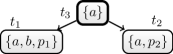
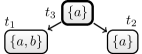
Figure 7: TD $\mathcal{T}$ (left) of the primal graph $G_{F}$ of Figure 6, and a TD $\mathcal{T^{\prime}}$ (right) of nested primal graph $G_{F}^{\{a,b\}}$.

Example 10.

Recall formula $F$, the tree decomposition $\mathcal{T}=(T,\chi)$ of $G_{F}$, as depicted in Figure 7 (left), and abstraction variables $A=\{a,b\}$ of Example 9. Consider TD $\mathcal{T}^{\prime}{\,\mathrel{\mathop{:}}=}(T,\chi^{\prime})$, where $\chi^{\prime}(t){\,\mathrel{\mathop{:}}=}\chi(t)\cap\{a,b\}$ for each node $t$ of $T$, which is given in Figure 7 (right). Observe that $\mathcal{T}^{\prime}$ is $\mathcal{T}$, but restricted to $A$ and that $\mathcal{T}^{\prime}$ is a TD of $G_{F}^{A}$ of width $1$. There are two compatible sets, namely $\{p_{1}\}$ and $\{p_{2}\}$. Observe that only for compatible set $U=\{p_{2}\}$ we have two nodes compatible with $U$, namely $t_{2}$ and $t_{3}$. We assume that $\operatorname{comp}_{F,A,\mathcal{T}^{\prime}}(U)=t_{2}$, i.e., we decide that $t_{2}$ shall be the unique node for $U$. Consequently, nested bag formulas are $F_{t_{1}}^{A}=\{c_{1},c_{2}\}$, $F_{t_{2}}^{A}=\{c_{3},c_{4}\}$, and $F_{t_{3}}^{A}{=}\emptyset$.

5.2 Nested Dynamic Programming on Abstractions

In: Nested table algorithm $\mathbb{N}$, nesting $\operatorname{depth}\geq 0$, instance $(F,P)$ of PMC, abstraction variables $A\subseteq\text{var}(F)$, and a TD $\mathcal{T}=(T,\chi)$ of the nested primal graph $G_{F}^{A}$.

Out: Table mapping $\mathbb{N}\text{-}\penalty 0\hskip 0.0pt\text{Comp}$, which maps each TD node $t$ of $T$ to some computed table $\tau_{t}$.

1

2$\mathbb{N}\text{-}\penalty 0\hskip 0.0pt\text{Comp}\leftarrow\{\}\qquad{\leavevmode\hbox{\set@color{{\hbox{/* }}}}\textnormal{{\ignorespaces empty mapping\hfill */}}}$

3for iterate $t$ in $\operatorname{post-order}(T)$ do

4     

5     $\text{Child-Tabs}\leftarrow\langle\mathbb{N}\text{-}\penalty 0\hskip 0.0pt\text{Comp}[t_{1}],\ldots,\mathbb{N}\text{-}\penalty 0\hskip 0.0pt\text{Comp}[t_{\ell}]\rangle\text{ where }\operatorname{children}(t)=\langle t_{1},\ldots,t_{\ell}\rangle$

6     $\mathbb{N}\text{-}\penalty 0\hskip 0.0pt\text{Comp}[t]\leftarrow{\mathbb{N}}(\operatorname{depth},t,\chi(t),F_{t},F_{t}^{A},P\cap\text{var}(F_{t}^{A}),\text{Child-Tabs})$

return $\mathbb{N}\text{-}\penalty 0\hskip 0.0pt\text{Comp}$

Listing 6 Algorithm ${\mathtt{NestDP}}_{\mathbb{N}}(\operatorname{depth},(F,P),A,\mathcal{T})$ for computing solutions of $(F,P)$ via nested DP on TD ${\mathcal{T}}$.

Now, we have established required notation in order to discuss nested dynamic programming (nested DP). Listing 6 presents algorithm $\mathtt{NestDP}$ for solving a given problem by means of nested dynamic programming. Observe that Listing 6 is almost identical to algorithm $\mathtt{DP}$ as presented in Listing 1. The reason for this is that nested dynamic programming can be seen as a refinement of dynamic programming, cf. algorithm $\mathtt{DP}$ of Listing 1. Indeed, the difference of $\mathtt{NestDP}$ compared to $\mathtt{DP}$ is that $\mathtt{NestDP}$ uses labeled tree decompositions of the nested primal graph and that it gets as additional parameter a set $A$ of abstraction variables. Further, instead of a table algorithm $\mathbb{A}$, algorithm $\mathtt{NestDP}$ relies on a nested table algorithm $\mathbb{N}$ during dynamic programming, which is similar to a table algorithm that gets as additional parameter an integer $\operatorname{depth}\geq 0$ that will be used later and a nested bag instance that needs to be evaluated. For simplicity and generality, also the formula is passed as a parameter, which is, however, used only for passing problem-specific information of the instance. Indeed, most nested table algorithm do not require this parameter, which should not be used for direct problem solving instead of utilizing the bag instance. Consequently, nested dynamic programming still follows the basic concept of dynamic programming as presented in Figure 2.

Similar to above, for the ease of presentation our presented nested table algorithms use nice tree decompositions only. However, this is not a hard restriction. Indeed, it is easy to see that for arbitrary TDs the clear case distinctions of nice decompositions are still valid, but are in general just overlapping. Further, without loss of generality we also assume that each compatible set $U$ gets assigned a unique node $t=\operatorname{comp}_{F,A,\mathcal{T}}(U)$ that is an introduce node, i.e., $\operatorname{type}(t)=\textit{int}$.

Nested Dynamic Programming for #Sat

In order to design a nested table algorithm for #Sat, assume a Boolean formula $F$ as well as a given labeled tree decomposition $\mathcal{T}=(T,\chi)$ of $G_{F}^{A}$ using any set $A$ of abstraction variables. Recall from the discussions above, that each variable $a\in\text{var}(F)\setminus A$ appears only in one nested bag formula $F_{t}^{A}$ of a node $t$ of $T$ that is unique for $a$. These unique variable appearances allow us to actually nest the evaluation of nested bag formula $F_{t}^{A}$. This evaluation is performed by a nested table algorithm ${\mathbb{N}\mathbb{SAT}}$ in the context of nested dynamic programming. Listing 7 shows this simple nested table algorithm ${\mathbb{N}\mathbb{SAT}}$ for solving problem #Sat by means of algorithm $\mathtt{NestDP}_{\mathbb{N}\mathbb{SAT}}$. For comparison, recall table algorithm $\mathbb{SAT}$ for solving problem #Sat by means of dynamic programming, as given by Listing 3. Observe that in contrast to Listing 3, we store here assignments (and not interpretations), which simplifies the presentation of nesting. However, the main difference of ${\mathbb{N}\mathbb{SAT}}$ compared to $\mathbb{SAT}$ is that the nested table algorithm ${\mathbb{N}\mathbb{SAT}}$ maintains a counter $c$ and that it gets called on a nested primal graph, i.e., the algorithm gets additional parameters like the nested bag formula. Then, the nested table algorithm evaluates this nested bag formula in Line 7 via any procedure #Sat for solving problem $\textsc{\#Sat}(F_{t}^{A}[J])$ on the nested bag formula $F_{t}^{A}$ simplified by the current assignment $J$ to variables in the bag $\chi(t)$. Note that this subproblem $\textsc{\#Sat}(F_{t}^{A}[J])$ itself can be solved by again using nested dynamic programming with the help of algorithm $\mathtt{NestDP}_{\mathbb{N}\mathbb{SAT}}$.

In: Node $t$, bag $\chi_{t}$, bag formula $F_{t}$, nested bag formula $F_{t}^{A}$, and sequence $\text{Child-Tabs}=\langle\tau_{1},\ldots\tau_{\ell}\rangle$ of child tables of $t$.

Out: Table $\tau_{t}.$

1 if $\operatorname{type}(t)=\textit{leaf}$ then $\tau_{t}\leftarrow\{\langle{\color[rgb]{0.62,0,0}\emptyset},{\color[rgb]{0,0.62,0}1}\rangle\}$;

2 else if $\operatorname{type}(t)=\textit{int}$ and $a\in\chi(t)$ is introduced then

3      $\tau_{t}\leftarrow\{\langle{\color[rgb]{0.62,0,0}J},{\color[rgb]{0,0.62,0}c^{\prime}\cdot c}\rangle$       $|\;\langle{\color[rgb]{0.62,0,0}I},{\color[rgb]{0,0.62,0}c}\rangle\in\tau_{1},J\in I\cup\{a\mapsto v\},v\in\{0,1\},J\vDash F_{t},c^{\prime}{>}0,c^{\prime}{=}$
$\textsc{\#Sat}(F_{t}^{A}[J])\}$

4else if $\operatorname{type}(t)=\textit{rem}$ and $a\not\in\chi(t)$ is removed then

     /* $\text{C}(I)$ is the set that contains the rows in $\tau_{1}$ for assignments $J$ that are equal to $I$ after removing $a$ */

5      $\text{C}(I)\leftarrow\{\langle J,c\rangle\mid\langle{J},{c}\rangle\in\tau_{1},J\setminus\{a\mapsto 0,a\mapsto 1\}=I\setminus\{a\mapsto 0,a\mapsto 1\}\}$

6      $\tau_{t}\leftarrow\{\langle{\color[rgb]{0.62,0,0}I\setminus\{a\mapsto 0,a\mapsto 1\}}$, $\sum_{\langle J,c\rangle\in C(I)}c\rangle\}$             $\mid\langle{\color[rgb]{0.62,0,0}I},{\color[rgb]{0,0.62,0}\cdot}\rangle\in\tau_{1}\}$;

7     

8 else if $\operatorname{type}(t)=\textit{join}$ then

9     $\tau_{t}\leftarrow\{\langle{\color[rgb]{0.62,0,0}I},{\color[rgb]{0,0.62,0}c_{1}\cdot c_{2}}\rangle$                           $|\;\langle{\color[rgb]{0.62,0,0}I},{\color[rgb]{0,0.62,0}c_{1}}\rangle\in\tau_{1},\langle{\color[rgb]{0.62,0,0}I},{\color[rgb]{0,0.62,0}c_{2}}\rangle\in\tau_{2}\}$

return $\tau_{t}$

Listing 7 Nested table algorithm ${\mathbb{N}\mathbb{SAT}}(\cdot,t,\chi_{t},F_{t},F_{t}^{A},\cdot,\text{Child-Tabs})$ for solving #Sat.

In the following, we briefly show the evaluation of nested dynamic programming for #Sat on an example.

Figure 8: Selected tables obtained by nested DP on TD ${\mathcal{T}}^{\prime}$ of $G_{F}^{\{a,b\}}$ (left) and on TD $\mathcal{T}^{\prime\prime}$ of $G_{F}^{\{a\}}$ (right) for $F$ of Example 10 via $\mathtt{NestDP}_{{\mathbb{N}\mathbb{SAT}}}$.

Example 11.

Recall formula $F$, set $A$ of abstraction variables, and TD $\mathcal{T}^{\prime}$ of nested primal graph $G_{F}^{A}$ given in Example 10. As already mentioned, Formula $F$ has six satisfying assignments, namely $\{a\mapsto 1,b\mapsto 0,p_{1}\mapsto 1,p_{2}\mapsto 0\}$, $\{a\mapsto 1,b\mapsto 0,p_{1}\mapsto 1,p_{2}\mapsto 1\}$, $\{a\mapsto 1,b\mapsto 1,p_{1}\mapsto 0,p_{2}\mapsto 0\}$, $\{a\mapsto 1,b\mapsto 1,p_{1}\mapsto 0,p_{2}\mapsto 1\}$, $\{a\mapsto 1,b\mapsto 1,p_{1}\mapsto 1,p_{2}\mapsto 0\}$, and $\{a\mapsto 1,b\mapsto 1,p_{1}\mapsto 1,p_{2}\mapsto 1\}$.

Figure 8 (left) shows TD $\mathcal{T}^{\prime}$ of $G_{F}^{A}$ and tables obtained by $\mathtt{NestDP}_{{\mathbb{N}\mathbb{SAT}}}(0,(F,\cdot),\allowbreak A,\mathcal{T}^{\prime})$ for model counting (#Sat) on $F$. We briefly discuss executing ${\mathbb{N}\mathbb{SAT}}$ on $\mathcal{T}^{\prime}$, resulting in tables $\tau_{1}$, $\tau_{2}$, and $\tau_{3}$ as shown in Figure 8 (left). Intuitively, table $\tau_{1}$ is the result of introducing variables $a$ and $b$. Recall from Example 10 that $F_{t_{1}}^{A}=\{c_{1},c_{2}\}$ with $c_{1}=\{\neg a,b,p_{1}\}$ and $c_{2}=\{a,\neg b,\neg p_{1}\}$. Then, in Line 7 of algorithm ${\mathbb{N}\mathbb{SAT}}$, for each assignment $I$ to $\{a,b\}$ of each row $r$ of $\tau_{1}$, we compute $\textsc{\#Sat}(F_{t_{1}}^{A}[I])$. Consequently, for assignment $I_{1}=\{a\mapsto 0,b\mapsto 0\}$, we have that there are two satisfying assignments of $F_{t_{1}}^{A}[I_{1}]$, namely $\{p_{1}\mapsto 0\}$ and $\{p_{1}\mapsto 1\}$. Indeed, this count of $2$ is obtained for the first row of table $\tau_{1}$ by Line 7. Analogously, one can derive the remaining tables of $\tau_{1}$ and one obtains table $\tau_{2}$ similarly, by using formula $F_{t_{2}}^{A}$. Then, table $\tau_{3}$ is the result of removing $b$ in node $t_{1}$ and combining agreeing assignments of rows accordingly. Consequently, we obtain that there are six satisfying assignments of $F$, which are all required to set $a$ to $1$ due to formula $F_{t_{2}}^{A}$ that is evaluated in node $t_{2}$.

Figure 8 (right) shows TD $\mathcal{T}^{\prime\prime}$ of $G_{F}^{\{a\}}$ and tables obtained by $\mathtt{NestDP}_{{\mathbb{N}\mathbb{SAT}}}(0,\allowbreak(F,\cdot),\allowbreak\{a\},\mathcal{T}^{\prime\prime})$ using TD $\mathcal{T}^{\prime\prime}$. Since $F_{t^{\prime\prime}}^{\{a\}}=F$ and $F[\{a\mapsto 0\}]$ is unsatisfiable, table $\tau_{t^{\prime\prime}}$ does not contain an entry corresponding to assignment $\{a\mapsto 0\}$, cf. Condition “$c^{\prime}{>}0$” in Line 7 of Listing 7. Thus, there are six satisfying assignments of $F_{t^{\prime\prime}}^{\{a\}}[\{a\mapsto 1\}]$ obtained by computing $\textsc{\#Sat}(F_{t^{\prime\prime}}^{\{a\}}[\{a\mapsto 1]\})$.

While the overall concept of nested dynamic programming as given by algorithm $\mathtt{NestDP}$ of Listing 6 is quite general, sometimes in practice it is sufficient to further restrict the set of choices for abstraction vertices $A$ when constructing the nested primal graph.

Nested Table Algorithm for PMC

To this end, we show the approach of nested dynamic programming for the problem PMC.

Example 12.

Recall formula $F$ as well as set $A=\{a,b\}$ of abstraction variables from Example 10. Then, we have that $(F,A)$ is an instance of the projected model counting problem PMC. Restricted to projection set $A$, the Boolean formula $F$ has two satisfying assignments, namely $\{a\mapsto 1,b\mapsto 0\}$ and $\{a\mapsto 1,b\mapsto 1\}$. Consequently, the solution to PMC on $(F,A)$, i.e., $\textsc{PMC}(F,A)$, is $2$.

Indeed, for solving projected model counting we mainly focus on the case, where for a given instance $(F,P)$ with Boolean formula $F$ of problem PMC, the abstraction variables $A$ that are used for constructing the nested primal graph $G_{F}^{A}$ are among the projection variables, i.e., $A\subseteq P$. The approach of nested DP can then be applied for solving projected model counting such that the nested table algorithm naturally extends algorithm $\mathbb{N}$$\mathbb{SAT}$ of Listing 7.

In: Node $t$, bag $\chi_{t}$, bag formula $F_{t}$, nested bag formula $F_{t}^{A}$, projection variables $P\subseteq\text{var}(F_{t}^{A})$, and sequence $\text{Child-Tabs}=\langle\tau_{1},\ldots\tau_{\ell}\rangle$ of child tables of $t$.

Out: Table $\tau_{t}.$

1 if $\operatorname{type}(t)=\textit{leaf}$ then $\tau_{t}\leftarrow\{\langle{\color[rgb]{0.62,0,0}\emptyset},{\color[rgb]{0,0.62,0}1}\rangle\}$;

2 else if $\operatorname{type}(t)=\textit{int}$ and $a\in\chi(t)$ is introduced then

3      $\tau_{t}\leftarrow\{\langle{\color[rgb]{0.62,0,0}J},{\color[rgb]{0,0.62,0}c^{\prime}\cdot c}\rangle$ $|\;\langle{\color[rgb]{0.62,0,0}I},{\color[rgb]{0,0.62,0}c}\rangle\in\tau_{1},=I\cup\{a\mapsto v\},v\in\{0,1\},J\vDash F_{t},c^{\prime}{>}0,c^{\prime}{=}$
$\textsc{PMC}(F_{t}^{A}[J],P)\}$

4else if $\operatorname{type}(t)=\textit{rem}$ and $a\not\in\chi(t)$ is removed then

5     $\text{C}(I)\leftarrow\{\langle J,c\rangle\mid\langle{J},{c}\rangle\in\tau_{1},J\setminus\{a\mapsto 0,a\mapsto 1\}=I\setminus\{a\mapsto 0,a\mapsto 1\}\}$

6      $\tau_{t}\leftarrow\{\langle{\color[rgb]{0.62,0,0}I\setminus\{a\mapsto 0,a\mapsto 1\}}$, $\sum_{\langle J,c\rangle\in C(I)}c$$\rangle$            $\mid\langle{\color[rgb]{0.62,0,0}I},{\color[rgb]{0,0.62,0}\cdot}\rangle\in\tau_{1}\}$;

7     

8 else if $\operatorname{type}(t)=\textit{join}$ then

9     $\tau_{t}\leftarrow\{\langle{\color[rgb]{0.62,0,0}I},{\color[rgb]{0,0.62,0}c_{1}\cdot c_{2}}\rangle$                           $|\;\langle{\color[rgb]{0.62,0,0}I},{\color[rgb]{0,0.62,0}c_{1}}\rangle\in\tau_{1},\langle{\color[rgb]{0.62,0,0}I},{\color[rgb]{0,0.62,0}c_{2}}\rangle\in\tau_{2}\}$

return $\tau_{t}$

Listing 8 Nested table algorithm $\mathbb{N}{{\mathbb{PMC}}}(\cdot,t,\chi_{t},F_{t},F_{t}^{A},P,\text{Child-Tabs})$ for solving PMC.

The nested table algorithm $\mathbb{N}$$\mathbb{PMC}$ for solving projected model counting via nested dynamic programming is presented in Listing 8. Observe that nested table algorithm $\mathbb{N}$$\mathbb{PMC}$ does not significantly differ from algorithm $\mathbb{N}$$\mathbb{SAT}$ due to $A\subseteq P$. Indeed, the main difference is only in Line 8 of Listing 7, where instead of a procedure for model counting, a procedure PMC for solving a projected model counting question is called.

5.3 Hybrid Dynamic Programming based on nested DP

Now, we have definitions at hand to further refine and discuss nested dynamic programming in the context of hybrid dynamic programming (hybrid DP), which combines using both standard solvers and parameterized solvers exploiting treewidth in the form of nested dynamic programming. We illustrate these ideas for the problem PMC next. Afterwards we discuss how to implement the resulting algorithms in order to efficiently solve PMC and #Sat by means of database management systems.

In: Nesting $\operatorname{depth}\geq 0$ and an instance $(F,P)$ of PMC.

Out: Number $\textsc{PMC}(F,P)$ of assignments.

1

2

3$(F^{\prime},P^{\prime})=\text{Preprocessing}(F,P)$

4$A\leftarrow P^{\prime}$

5 if $F^{\prime}\in\operatorname{dom}(\operatorname{cache})\quad{\leavevmode\hbox{\set@color{{\hbox{/* }}}}\textnormal{{\ignorespaces Cache Hit\hfill */}}}\qquad$ then return $\operatorname{cache}(F^{\prime})\cdot 2^{|P\setminus P^{\prime}|}$;

6

7if $P^{\prime}=\emptyset$ then return $\textsc{Sat}(F^{\prime})\cdot 2^{|P|}$;

8 $\mathcal{T}=(T,\chi)\leftarrow\text{Decompose\_via\_Heuristics}(G_{F^{\prime}}^{A})\qquad{\leavevmode\hbox{\set@color{{\hbox{/* }}}}\textnormal{{\ignorespaces Decompose\hfill */}}}$

9if $\operatorname{width}(\mathcal{T})\geq\text{threshold}_{\text{hybrid}}\text{ or }\operatorname{depth}\geq\text{threshold}_{\text{depth}}$ /* Standard Solver */ then

10      if $\text{var}(F^{\prime})=P^{\prime}$ then $\operatorname{cache}\leftarrow\operatorname{cache}\cup\{(F^{\prime},\textsc{\#Sat}(F^{\prime}))\}$;

11      else          $\operatorname{cache}\leftarrow\operatorname{cache}\cup\{(F^{\prime},\textsc{PMC}(F^{\prime},P^{\prime}))\}$;

12      return $\operatorname{cache}(F^{\prime})\cdot 2^{|P\setminus P^{\prime}|}$

13

14

15if $\operatorname{width}(\mathcal{T})\geq\text{threshold}_{\text{abstr}}\,{\leavevmode\hbox{\set@color{{\hbox{/* }}}}\textnormal{{\ignorespaces Abstract via Heuristics \& Decompose\hfill */}}}\,$ then

16      $A\quad\,\,\,\,\,\leftarrow\text{Choose\_Subset\_via\_Heuristics}(A,F^{\prime})$

17     $\mathcal{T}=(T,\chi)\leftarrow\text{Decompose\_via\_Heuristics}(G_{F^{\prime}}^{A})$

18

19

20$\mathbb{N}\text{-}\penalty 0\hskip 0.0pt\text{Comp}\leftarrow\mathtt{NestDP}_{\mathbb{H}{{\mathbb{PMC}}}}(\operatorname{depth},(F^{\prime},P^{\prime}),A,\mathcal{T})\,{\leavevmode\hbox{\set@color{{\hbox{/* }}}}\textnormal{{\ignorespaces Nested Dynamic Programming\hfill */}}}$

21$\operatorname{cache}\leftarrow\operatorname{cache}\cup\{(F^{\prime},c)\mid\langle\emptyset,c\rangle\in\mathbb{N}\text{-}\penalty 0\hskip 0.0pt\text{Comp}[\operatorname{root}(T)]\}$

return $\operatorname{cache}(F^{\prime})\cdot 2^{|P\setminus P^{\prime}|}$

Listing 9 Algorithm $\mathtt{HybDP}_{\mathbb{H}{{\mathbb{PMC}}}}(\operatorname{depth},F,P)$ for hybrid DP of PMC based on nested DP.

Listing 9 depicts our algorithm $\mathtt{HybDP}_{\mathbb{H}{{\mathbb{PMC}}}}$ for solving projeceted model counting, i.e., problem PMC. This algorithm $\mathtt{HybDP}_{\mathbb{H}{{\mathbb{PMC}}}}$ takes an instance $(F,P)$ of PMC consisting of Boolean formula $F$ and projection variables $P$. The algorithm maintains a global, but simple $\operatorname{cache}$ mapping a formula to an integer, and consists of the following four subsequent blocks of code, which are separated by empty lines: (1) Preprocessing & Cache Consolidation, (2) Standard Solving, (3) Abstraction & Decomposition, and (4) Nested Dynamic Programming, which causes an indirect recursion through nested table algorithm $\mathbb{H}$$\mathbb{PMC}$, as discussed later.

Block (1) spans Lines 9 -9 and performs simple preprocessing techniques [69] like unit propagation, thereby obtaining a simplified instance $(F^{\prime},P^{\prime})$, where simplified formula $F^{\prime}$ of $F$ and projection variables $P^{\prime}\subseteq P$ are obtained. Any preprocessing simplifications are fine, as long as the solution of the resulting PMC instance $(F^{\prime},P^{\prime})$ is the same as solving PMC on $(F,P)$. Then, in Line 9, we set the set $A$ of abstraction variables to $P^{\prime}$, and consolidate $\operatorname{cache}$ with the updated formula $F^{\prime}$. Note that the operations in Line 9 are required to return a simplified instance that preserves satisfying assignments of the original formula when restricted to $P$. If $F^{\prime}$ is not cached, in Block (2), we do standard solving if the width is out-of-reach for nested DP, which spans over Lines 9-9. More precisely, if the updated formula $F^{\prime}$ does not contain projection variables, in Line 9 we employ a Sat solver returning integer $1$ or $0$. If $F^{\prime}$ contains projection variables and either the width obtained by heuristically decomposing $G_{F^{\prime}}$ is above $\text{threshold}_{\text{hybrid}}$, or the nesting depth exceeds $\text{threshold}_{\text{depth}}$, we use a standard #Sat or PMC solver depending on $P^{\prime}$.

Block (3) spans Lines 9-9 and is reached if no cache entry was found in Block (1) and standard solving was skipped in Block (2). If the width of the computed decomposition is above $\text{threshold}_{\text{abstr}}$, we need to use an abstraction in form of the nested primal graph. This is achieved by choosing suitable subsets $E\subseteq A$ of abstraction variables and decomposing ${F}_{t}^{E}$ heuristically.

Finally, Block (4) concerns nested DP, cf. Lines 9-9. This block relies on nested table algorithm $\mathbb{H}{{\mathbb{PMC}}}$, which is given in Listing 10 that is almost identical to nested table algorithm $\mathbb{N}{{\mathbb{PMC}}}$ as already discussed above and given in Listing 8. The only difference of $\mathbb{H}{{\mathbb{PMC}}}$ compared to $\mathbb{N}{{\mathbb{PMC}}}$ is that in Line 10 the nested table algorithm $\mathbb{H}{{\mathbb{PMC}}}$ uses the parameter $\operatorname{depth}$ and recursively executes algorithm $\mathtt{HybDP}_{\mathbb{H}{{\mathbb{PMC}}}}$ on the increased nesting depth of $\operatorname{depth}+1$, and the same formula as the one used in the generic PMC oracle call in Line 8 of Listing 8.

As a result, our approch deals with high treewidth by recursively finding and decomposing abstractions of the graph. If the treewidth is too high for some parts, tree decompositions of abstractions are used to guide standard solvers. Towards defining an actual implementation for practical solving, one still needs to find values for the threshold constants $\text{threshold}_{\text{hybrid}}$, $\text{threshold}_{\text{depth}}$, and $\text{threshold}_{\text{abstr}}$. The actual values of these constants will be made more precisely in the next section when discussing our implementation and experiments.

Figure 9: Selected tables obtained by nested DP using $\mathtt{NestDP}_{\mathbb{H}{{\mathbb{PMC}}}}$ on TD ${\mathcal{T}}^{\prime}$ of $G_{F}^{\{a,b\}}$ (left) and on TD $\mathcal{T}^{\prime\prime}$ of $G_{F}^{\{a\}}$ (right) for instance $(F,\{a,b\})$ of Example 12.

In: Nesting $\operatorname{depth}\geq 0$, node $t$, bag $\chi_{t}$, bag formula $F_{t}$, nested bag formula $F_{t}^{A}$, projection variables $P\subseteq\text{var}(F_{t}^{A})$, and sequence $\text{Child-Tabs}=\langle\tau_{1},\ldots\tau_{\ell}\rangle$ of child tables of $t$.

Out: Table $\tau_{t}.$

1 if $\operatorname{type}(t)=\textit{leaf}$ then $\tau_{t}\leftarrow\{\langle{\color[rgb]{0.62,0,0}\emptyset},{\color[rgb]{0,0.62,0}1}\rangle\}$;

2 else if $\operatorname{type}(t)=\textit{int}$ and $a\in\chi(t)$ is introduced then

3      $\tau_{t}\leftarrow\{\langle{\color[rgb]{0.62,0,0}J},{\color[rgb]{0,0.62,0}c^{\prime}{\cdot}c}\rangle$ $|\;\langle{\color[rgb]{0.62,0,0}I},{\color[rgb]{0,0.62,0}c}\rangle\in\tau_{1},J=I\cup\{a\mapsto v\},v\in\{0,1\},J\vDash F_{t},c^{\prime}>0,c^{\prime}{=}$
$\mathtt{HybDP}_{\mathbb{H}{{\mathbb{PMC}}}}(\operatorname{depth}{+}1,F_{t}^{A}[J],P)\}$

4else if $\operatorname{type}(t)=\textit{rem}$ and $a\not\in\chi(t)$ is removed then

5     $\text{C}(I)\leftarrow\{\langle J,c\rangle\mid\langle{J},{c}\rangle\in\tau_{1},J\setminus\{a\mapsto 0,a\mapsto 1\}=I\setminus\{a\mapsto 0,a\mapsto 1\}\}$

6      $\tau_{t}\leftarrow\{\langle{\color[rgb]{0.62,0,0}I\setminus\{a\mapsto 0,a\mapsto 1\}}$, $\sum_{\langle J,c\rangle\in C(I)}c$$\rangle$            $\mid\langle{\color[rgb]{0.62,0,0}I},{\color[rgb]{0,0.62,0}\cdot}\rangle\in\tau_{1}\}$;

7     

8 else if $\operatorname{type}(t)=\textit{join}$ then

9     $\tau_{t}\leftarrow\{\langle{\color[rgb]{0.62,0,0}I},{\color[rgb]{0,0.62,0}c_{1}\cdot c_{2}}\rangle$                           $|\;\langle{\color[rgb]{0.62,0,0}I},{\color[rgb]{0,0.62,0}c_{1}}\rangle\in\tau_{1},\langle{\color[rgb]{0.62,0,0}I},{\color[rgb]{0,0.62,0}c_{2}}\rangle\in\tau_{2}\}$

return $\tau_{t}$

Listing 10 Nested table algorithm $\mathbb{H}{{\mathbb{PMC}}}(\operatorname{depth},t,\chi_{t},F_{t},F_{t}^{A},P,\text{Child-Tabs})$ for solving PMC.

Example 13.

Recall instance $(F,A)$ of Example 12, and set $A$ of abstraction variables as well as TD $\mathcal{T}^{\prime}$ of nested primal graph $G_{F}^{A}$ as given in Example 10. Further, recall that restricted to projection set $A$, formula $F$ has two satisfying assignments. Figure 9 (left) shows TD $\mathcal{T}^{\prime}$ of $G_{F}^{A}$ and tables obtained by $\mathtt{NestDP}_{\mathbb{H}{{\mathbb{PMC}}}}(0,(F,A),A,\mathcal{T}^{\prime})$ for solving projected model counting on $(F,A)$.

Note that nested table algorithm $\mathbb{H}{{\mathbb{PMC}}}$ of Listing 10 works similar to the nested table algorithm $\mathbb{N}$$\mathbb{PMC}$ of Listing 8, but it calls $\mathtt{HybDP}_{\mathbb{H}{{\mathbb{PMC}}}}$ recursively. We briefly discuss executing $\mathbb{H}{{\mathbb{PMC}}}$ in the context of Line 9 of algorithm $\mathtt{HybDP}_{\mathbb{H}{{\mathbb{PMC}}}}$ on node $t_{1}$, resulting in table $\tau_{1}$ as shown in Figure 9 (left). Recall that $F_{t_{1}}^{A}=\{\{\neg a,b,p_{1}\},\{a,\neg b,\neg p_{1}\}\}$. Then, in Line 10 of algorithm $\mathbb{H}{{\mathbb{PMC}}}$, for each assignment $J$ to $\{a,b\}$ of each row of $\tau_{1}$, we compute $\mathtt{HybDP}_{\mathbb{H}{{\mathbb{PMC}}}}(\operatorname{depth}+1,F_{t_{1}}^{A}[J],\emptyset)$. Each of these recursive calls, however, is already solved by unit propagation (preprocessing), e.g., $F_{t_{1}}^{A}[\{a\mapsto 1,b\mapsto 0\}]$ of Row 2 simplifies to $\{\{p_{1}\}\}$.

Figure 9 (right) shows TD $\mathcal{T}^{\prime\prime}$ of $G_{F}^{E}$ with $E{\,\mathrel{\mathop{:}}=}\{a\}$, and tables obtained by algorithm $\mathtt{NestDP}_{\mathbb{H}{{\mathbb{PMC}}}}(0,(F,A),E,\mathcal{T}^{\prime\prime})$. Still, $F_{t^{\prime\prime}}^{E}[J]$ for a given assignment $J$ to $\{a\}$ of any row $r\in\tau_{t^{\prime\prime}}$ can be simplified. Concretely, $F_{t^{\prime\prime}}^{E}[\{a\mapsto 0\}]$ evaluates to $\emptyset$ and $F_{t^{\prime\prime}}^{E}[\{a\mapsto 1\}]$ evaluates to clause $\{b,c\}$. Thus, restricted to $\{b\}=A\setminus\{a\}$, there are 2 satisfying assignments $\{b\mapsto 0\}$, $\{b\mapsto 1\}$ of $F_{t^{\prime\prime}}^{E}[\{a\mapsto 1\}]$.

6 Hybrid Dynamic Programming in Practice

Below, in Section 6.1 we present an implementation of hybrid dynamic programming in order to solve the problems #Sat as well as PMC. This is then followed by an experimental evaluation and discussion of the results in Section 6.2, where we also briefly elaborate on existing techniques of state-of-the-art solvers.

6.1 Implementing Hybrid Dynamic Programming

We implemented a solver nestHDB based on hybrid dynamic programming in Python3 and using table manipulation techniques by means of structured query language (SQL) and the database management system (DBMS) PostgreSQL. Our solver builds upon the recently published prototype dpdb [39], which applied a DBMS for the efficient implementation of plain dynamic programming algorithms. This dpdb prototype provides a basic framework for implementing plain dynamic programming algorithms, which can be specified in the form of a plain table algorithm, e.g., the one of Listing 3. However, this system does not have support for neither hybrid nor nested dynamic programming. In order to compare plain dpdb and our solver nestHDB in a fair way, for both systems we used the most-recent version 12 of PostgreSQL and we let it operate on a tmpfs-ramdisk instead of disk space (HDD/SDD), i.e., within the main memory (RAM) of a machine. In both dpdb as well as our solver nestHDB, the DBMS serves the purpose of extremely efficient in-memory table manipulations and query optimization required by nested DP, and therefore nestHDB benefits from database technology. Those benefits are already available in the form of different and efficient join manipulations that are selected based on several heuristics that are invoked during SQL query optimizing. Note that especially efficient join operations have been already designed, implemented, combined, and tuned for decades [70, 71, 72]. Therefore it seems more than natural to rely on this technological advancement that database theory readily provides. We are certain that one can easily replace PostgreSQL by any other state-of-the-art relational database that uses standard SQL in order to express queries. In the following, we briefly discuss implementation specifics that are crucial for a performant system that is competitive with state-of-the-art solvers.

Nested DP & Choice of Standard Solvers. We implemented dedicated nested DP algorithms for solving #Sat and PMC, where we do (nested) DP up to $\text{threshold}_{\text{depth}}=2$. Note that incrementing nesting depth results in getting again exponentially many (in the largest bag size) rows for each row of tables of the previous depth, i.e., a low nesting limit is highly expected. Currently, we do not see a way to efficiently solve instances of higher nesting depth, which might change in case of further advances allowing to decrease table sizes obtained during dynamic programming. Further, we set $\text{threshold}_{\text{hybrid}}=1000$ and therefore we do not “fall back” to standard solvers based on the width (cf., Line 9 of Listing 9), but based on the nesting depth.

Also, the evaluation of the nested bag formula is “shifted” to the database if it uses at most $40$ abstraction variables, since PostgreSQL efficiently handles these small-sized Boolean formulas. Thereby, further nesting is saved by executing optimized SQL statements within the TD nodes. A value of 40 seems to be a nice balance between the overhead caused by standard solvers for small formulas and exponential growth counteracting the advantages of the DBMS. For hybrid solving, we use #Sat solver SharpSAT [73] and for PMC we employ the recently published PMC solver projMC [20], solver SharpSAT and Sat solver picosat [74]. Observe that our solver immediately benefits from better standard solvers and further improvements of the solvers above.

Choosing Non-Nesting Variables & Compatible Nodes. TDs are computed by means of heuristics via decomposition library htd [36]. We implement a heuristic for finding practically sufficient abstractions, i.e., abstraction variables for the nested primal graph, in reasonable using an external solver. Therefore, we encode our heuristic into two logic programs (ASP) for solver clingo [75], which includes techniques for fast solving reachability via nesting paths. The encodings, which in total comprise 11 lines, are publicly available in the online repository of nestHDB. Technically, our focus is on avoiding extremely large abstractions at the cost of larger nested bag formulas. Still, nesting allows to obtain refined abstractions again at higher depths. Thereby, we achieve a good trade off between runtime and quality.

By the first encoding (“guess_min_degree.lp”), we compute a reasonably-sized subset of vertices of smallest degree, more precisely, such that the number of neighboring vertices not in the set is minimized. We take a subset of size at most $95$, which turned out to be practically useful. We run the ASP solver clingo for up to $10$ seconds. The solver might not return an optimum within $10$ seconds, but always returns a subset of vertices that can be used subsequently.

By the second encoding (“guess_increase.lp”), we guess among the thereby obtained subset of vertices of preferably smallest degree, a preferably maximal set $A$ of at most $64$ abstraction variables such the resulting graph $G_{F}^{A}$ is reasonably sparse, which is achieved by minimizing the number of edges of $G_{F}^{A}$. To this end, we also use built-in (cost) optimization, where we take the best results obtained by clingo after running at most 35 seconds. For more details on ASP, we refer to introductory texts [26, 75].

We expect that this approach, which driven mostly by practical considerations, can be improved. Furthermore, it can also be extending by problem-specific as well as domain-specific information, which might help in choosing promising abstraction variables $A$.

As rows of tables during (nested) DP can be independently computed and parallelized [40], hybrid solver nestHDB potentially calls standard solvers for solving subproblems in parallel using a thread pool. Thereby, the uniquely compatible node for relevant compatible sets $U$, as denoted in this paper by means of $\operatorname{comp}(\cdot)$, is decided during runtime among compatible nodes on a first-come-first-serve basis.

6.2 Experimental Evaluation

In order to evaluate the concept of hybrid dynamic programming, we conducted a series of experiments considering a variety of solvers and benchmarks, both for model counting (#Sat) as well as projected model counting (PMC). During the evaluation we thereby compared the performance of algorithm $\mathtt{HybDP}_{\mathbb{H}{{\mathbb{PMC}}}}$ of Listing 9. We benchmarked this algorithm both for the projected model counting problem, but also for the special case of model counting, where all variables are projection variables.

Figure 10: Cactus plot of instances for #Sat, where instances (x-axis) are ordered for each solver individually by runtime[seconds] (y-axis). $\text{threshold}_{\text{abstr}}=38$.

Benchmarked Solvers & Instances

We benchmarked nestHDB and 16 other publicly available #Sat solvers on 1,494 instances recently considered [39]. Most of the existing solvers of other approaches are single-core solvers, which adhere to three different techniques, namely knowledge-compilation based, caching based, and approximate. Among the knowledge-compilation based solvers, which aim to obtain compact representations of the formulas that are concise and easier to solve, are miniC2D [76], d4 [14], c2d [77], sdd [78], dsharp [79], cnf2eadt [80], and bdd_minisat [81]. These solvers use different variants and flavors of knowledge-compilation, thereby finding decent trade-offs between the time needed to obtain those representations and their succinctness. We also considered the caching-based solvers cachet [82], sharpSAT [73], and ganak [83], which employ existing Sat-based solvers by sophisticated caching techniques. Finally, among the approximate counters, we focused on sts [84], sharpCDCL [85], and approxmc3 [86], which employ sampling-based techniques to approximately obtain the model counts. Our comparison also included the multi-core solvers dpdb [39], gpusat2 [40], which is also based on dynamic programming and uses massively parallel graphics processing units (GPUs), as well as countAntom [87], which relies on sophisticated techniques for work-balancing. For a more ample description of the used techniques, we refer to the model counting competition report [19]. Note that we excluded distributed solvers such as dCountAntom [88] and DMC [89] from our experimental setup. Both solvers require a cluster with access to the OpenMPI framework [90] and fast physical interconnections. Unfortunately, we do not have access to OpenMPI on our cluster. Nonetheless, our focus are shared-memory systems and since dpdb might well be used in a distributed setting, it leaves an experimental comparison between distributed solvers that also include dpdb as subsolver to future work. While nestHDB itself is a multi-core solver, we additionally included in our comparison nestHDB(sc), which is nestHDB, but restricted to a single core only. The instances [39] we took are already preprocessed by pmc [69] using recommended options -vivification -eliminateLit -litImplied -iterate=10 -equiv -orGate -affine, which guarantee that the model counts are preserved. However, nestHDB still uses pmc with these options in Line 9 of Listing 9, which is used in the light of nested bag formulas that appear due to nesting.

Further, we considered the problem PMC, where we compare solvers projMC [20], clingo [75], ganak [83], nestHDB ${}^{\ref{foot:source}}$, and nestHDB(sc) on 610 publicly available instances from projMC (consisting of 15 planning, 60 circuit, and 100 random instances) and Fremont, with 170 symbolic-markov applications, and 265 misc instances. For simplifying nested bag formulas under assignments encountered due to nesting in Line 9 of Listing 9, nestHDB uses pmc as before, but without options -equiv -orGate -affine to ensure preservation of models (equivalence).

bench-	solver	tw upper bound					$\sum$	time
mark set		max	0-30	31-50	$>$50			[h]
planning	nestHDB	30	7	0	0		7	2.88
	nestHDB(sc)	30	7	0	0		7	3.31
	projMC	26	6	0	0		6	3.01
	ganak	19	5	0	0		5	3.36
	clingo	4	1	0	0		1	4.00
circ	nestHDB	99	34	10	16		60	2.10
	nestHDB(sc)	99	34	4	14		52	4.60
	projMC	91	28	10	11		49	6.23
	ganak	99	34	10	16		60	1.21
	clingo	99	31	10	16		57	4.44
random	nestHDB	79	30	20	17		67	10.91
	nestHDB(sc)	79	30	20	15		65	11.29
	projMC	84	30	20	15		65	11.09
	ganak	19	19	0	0		19	23.18
	clingo	24	25	0	0		25	21.38
markov	nestHDB	23	62	0	0		62	31.98
	nestHDB(sc)	23	61	0	0		61	32.54
	projMC	8	54	0	0		54	33.65
	ganak	59	64	0	4		68	30.32
	clingo	3	38	0	0		38	37.54
misc	nestHDB	47	38	17	0		55	46.12
	nestHDB(sc)	47	38	13	0		51	48.20
	projMC	47	38	13	0		51	45.90
	ganak	44	38	15	0		53	45.72
	clingo	63	38	15	1		54	44.79
$\Sigma$	nestHDB	99	171	47	33		251	93.99
	nestHDB(sc)	99	170	37	29		236	99.95
	projMC	91	156	43	26		225	99.88
	ganak	99	160	25	20		205	103.78
	clingo	99	133	25	17		175	112.15

Figure 11: Number of solved PMC instances, grouped by upper bound intervals of treewidth. time[h] is cumulated wall clock time, timeouts count as 900s. $\text{threshold}_{\text{abstr}}{=}8$.

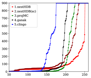
Figure 12: Cactus plot showing the number of solved PMC instances, where the x-axis shows for each solver (configuration) individually, the number of instances ordered by increasing runtime. time[h] is cumulated wall clock time, timeouts count as 900s. $\text{threshold}_{\text{abstr}}{=}8$.

Benchmark Setup

Solvers ran on a cluster of 12 nodes. Each node of the cluster is equipped with two Intel Xeon E5-2650 CPUs consisting of 12 physical cores each at 2.2 GHz clock speed, 256 GB RAM. For dpdb and nestHDB, we used PostgreSQL 12 on a tmpfs-ramdisk (/tmp) that could grow up to at most 1 GB per run. Results were gathered on Ubuntu 16.04.1 LTS machines with disabled hyperthreading on kernel 4.4.0-139. We mainly compare total wall clock time and number of timeouts. For parallel solvers (dpdb, countAntom, nestHDB) we allow 12 physical cores. Timeout is 900 seconds and RAM is limited to 16 GB per instance and solver. Results for gpusat2 are taken from [39], where a machine equipped with a consumer GPU is used: Intel Core i3-3245 CPU operating at 3.4 GHz, 16 GB RAM, and one Sapphire Pulse ITX Radeon RX 570 GPU running at 1.24 GHz with 32 compute units, 2048 shader units, and 4GB VRAM using driver amdgpu-pro-18.30-641594 and OpenCL 1.2. The system operated on Ubuntu 18.04.1 LTS with kernel 4.15.0-34.

Benchmark Results

The results for #Sat showing the best 14 solvers are summarized in the cactus plot of Figure 10. Overall it shows nestHDB among the best solvers, solving 1,273 instances. The reason for this is, compared to dpdb, that nestHDB can solve instances using TDs of primal graphs of widths larger than 44, up to width 266. This limit is even slightly larger than the width of 264 that SharpSAT on its own can handle. We also tried using minic2d instead of SharpSAT as standard solver for solvers nestHDB and nestHDB(sc), but we could only solve one instance more. Notably, nestHDB(sc) has about the same performance as nestHDB, indicating that parallelism does not help much on the instances. Further, we observed that the employed simple cache as used in Listing 9, provides only a marginal improvement.

Figure 11 depicts a table of results on PMC, where we observe that nestHDB does a good job on instances with low widths below $\text{threshold}_{\text{abstr}}=8$ (containing ideas of dpdb), but also on widths well above $8$ (using nested DP). Notably, nestHDB is also competitive on widths well above $50$. Indeed, nestHDB and nestHDB(sc) perform well on all benchmark sets, whereas on some sets the solvers projMC, clingo and ganak are faster. Overall, parallelism provides a significant improvement here, but still nestHDB(sc) shows competitive performance, which is also visualized in the cactus plot of Figure 12. Figure 13 shows scatter plots comparing nestHDB to projMC (left) and to ganak (right). Overall, both plots show that nestHDB solves more instances, since in both cases the y-axis shows more black dots at 900 seconds than the x-axis. Further, the bottom left of both plots shows that there are plenty easy instances that can be solved by projMC and ganak in well below 50 seconds, where nestHDB needs up to 200 seconds. Similarly, the cactus plot given in Figure 12 shows that nestHDB can have some overhead compared to the three standard solvers, which is not surprising. This indicates that there is still room for improvement if, e.g., easy instances are easily detected, and if standard solvers are used for those instances. Alternatively, one could also just run a standard solver for at most 50 seconds and if not solved within 50 seconds, the heavier machinery of nested dynamic programming is invoked. Apart from these instances, Figure 13 shows that nestHDB solves harder instances faster, where standard solvers struggle.

Figure 13: Scatter plot of instances for PMC, where the x-axis shows runtime in seconds of nestHDB compared to the y-axis showing runtime of projMC (left) and of ganak (right). $\text{threshold}_{\text{abstr}}=8$.

7 Discussion and Conclusion

We introduced a dynamic programming algorithm to solve projected model counting (PMC) by exploiting the structural parameter treewidth. Our algorithm is asymptotically optimal under the exponential time hypothesis (ETH). Its runtime is double exponential in the treewidth of the primal graph of the instance and polynomial in the size of the input instance. We believe that our results can also be extended to another graph representation, namely the incidence graph. Our approach is very general and might be applicable to a wide range of other hard combinatorial problems, such as projection for ASP [56] and QBF [91].

Then, in order to still efficiently deal with projected model counting in practice, we presented nested dynamic programming (nested DP) using different levels of abstractions, which are subsequently refined and solved recursively. This approach is complemented with hybrid solving, where (search-intense) subproblems are solved by standard solvers. We provided nested DP algorithms for problems related to Boolean satisfiability, but the idea can be easily applied for other formalisms. We implemented some of these algorithms and our benchmark results are promising.

In the light of related works on properties for efficient counting algorithms, e.g., [32, 33, 34], we are curious to revisit some of those and potentially study precise runtime dependencies. We expect interesting insights when focusing on the search for properties of local instance parts that in combination with treewidth allow algorithms that are significantly better than double-exponential in the treewidth. As we demonstrated in the experimental results, we can solve the problem PMC that theoretically requires double-exponential worst-case effort in the treewidth, on instances of decent treewidth upper bounds (up to 99). On plain model counting (#Sat), which is only single-exponential in the treewidth, our solver even deals with instances of larger treewidth upper bounds (up to 260). This also opens the question of whether similar empirical observations can be drawn in other areas and formalisms like constraint solving or database query languages. Further, we plan on deeper studies of problem-specific abstractions, in particular for quantified Boolean formulas. We want to further tune our solver parameters (e.g., thresholds, timeouts, sizes), deepen interleaving with PMC solvers like projMC, and to use incremental solving for obtaining abstractions and evaluating nested bag formulas, where intermediate solver references are kept during dynamic programming and formulas are iteratively added and (re-)solved.

Appendix A Omitted Proofs

Observation 1.

The relation $\operatorname{=_{P}}$ is an equivalence relation.

Proof.

One can easily see that $=_{P}(A,B){\,\mathrel{\mathop{:}}=}(A\cap P)=(B\cap P)$ is

• reflexive: $A\cap P=A\cap P$ for any two sets $A,P$,

• symmetric: $A\cap P=B\cap P$ if and only if $B\cap P=A\cap P$ for given sets $A,B,P$, and

• transitive: if $A\cap P=B\cap P$ and $B\cap P=C\cap P$, then $A\cap P=C\cap P$ holds as well for any sets $A,B,C,P$.

As a result, $=_{P}$ is an equivalence relation. ∎

Observation 3.

Let $n$ be a positive integer, $X=\{1,\ldots,n\}$, and $X_{1}$, $X_{2}$, $\ldots$, $X_{n}$ subsets of $X$. The number of elements in the intersection over all sets $A_{i}$ is

$$|\bigcap_{i\in X}X_{i}|= \Bigg{|}|\bigcup^{n}_{j=1}X_{j}| -\sum_{\emptyset\subsetneq I\subsetneq X,|I|=1}|\bigcap_{i\in I}X_{i}|+\sum_{\emptyset\subsetneq I\subsetneq X,|I|=2}|\bigcap_{i\in I}X_{i}|-\ldots$$

$$+\sum_{\emptyset\subsetneq I\subsetneq X,|I|=n-1}(-1)^{|I|}|\bigcap_{i\in I}X_{i}|\Bigg{|}.$$

It trivially works to count arbitrary sets.

Proof.

We take the well-known inclusion-exclusion principle [46] and rearrange the equation.

$$|\bigcup^{n}_{j=1}X_{j}|= \sum_{\emptyset\subsetneq I\subseteq X}(-1)^{|I|-1} |\bigcap_{i\in I}X_{i}|$$

$$|\bigcup^{n}_{j=1}X_{j}|= \sum_{\emptyset\subsetneq I\subsetneq X}(-1)^{|I|-1} |\bigcap_{i\in I}X_{i}|+(-1)^{|X|-1}|\bigcap_{i\in X}X_{i}|$$

$$(-1)^{|X|-1}|\bigcap_{i\in X}X_{i}|= |\bigcup^{n}_{j=1}X_{j}|-\sum_{\emptyset\subsetneq I\subsetneq X}(-1)^{|I|-1}|\bigcap_{i\in I}X_{i}|$$

$$|\bigcap_{i\in X}X_{i}|= \Bigg{|} |\bigcup^{n}_{j=1}X_{j}|-\sum_{\emptyset\subsetneq I\subsetneq X}(-1)^{|I|-1}|\bigcap_{i\in I}X_{i}|\Bigg{|}$$

$$|\bigcap_{i\in X}X_{i}|= \Bigg{|} |\bigcup^{n}_{j=1}X_{j}|-\sum_{\emptyset\subsetneq I\subsetneq X,|I|=1}|\bigcap_{i\in I}X_{i}|$$

$$+\sum_{\emptyset\subsetneq I\subsetneq X,|I|=2}|\bigcap_{i\in I}X_{i}|$$

$$-\ldots$$

$$+\sum_{\emptyset\subsetneq I\subsetneq X,|I|=n-1}(-1)^{|I|}|\bigcap_{i\in I}X_{i}|\Bigg{|}$$

∎

References

- [1] B. Abramson, J. Brown, W. Edwards, A. Murphy, R. L. Winkler, Hailfinder: A Bayesian system for forecasting severe weather, International Journal of Forecasting 12 (1) (1996) 57–71. doi:10.1016/0169-2070(95)00664-8.
- [2] A. Choi, G. Van den Broeck, A. Darwiche, Tractable learning for structured probability spaces: A case study in learning preference distributions, in: Q. Yang (Ed.), Proceedings of 24th International Joint Conference on Artificial Intelligence (IJCAI’15), The AAAI Press, 2015.
- [3] C. Domshlak, J. Hoffmann, Probabilistic planning via heuristic forward search and weighted model counting, J. Artif. Intell. Res. 30 (2007) 565–620. doi:10.1613/jair.2289.
- [4] L. Dueñas-Osorio, K. S. Meel, R. Paredes, M. Y. Vardi, Counting-based reliability estimation for power-transmission grids, in: S. P. Singh, S. Markovitch (Eds.), Proceedings of the Thirty-First AAAI Conference on Artificial Intelligence (AAAI’17), The AAAI Press, San Francisco, CA, USA, 2017, pp. 4488–4494.
- [5] C. D. Manning, P. Raghavan, H. Schütze, Introduction to Information Retrieval, Cambridge University Press, Cambridge, 2008.
- [6] O. Pourret, P. Naim, M. Bruce, Bayesian Networks - A Practical Guide to Applications, John Wiley & Sons, 2008.
- [7] M. Sahami, S. Dumais, D. Heckerman, E. Horvitz, A Bayesian approach to filtering junk e-mail, in: T. Joachims (Ed.), Proceedings of the AAAI-98 Workshop on Learning for Text Categorization, Vol. 62, 1998, pp. 98–105.
- [8] T. Sang, P. Beame, H. Kautz, Performing Bayesian inference by weighted model counting, in: M. M. Veloso, S. Kambhampati (Eds.), Proceedings of the 29th National Conference on Artificial Intelligence (AAAI’05), The AAAI Press, 2005.
- [9] Y. Xue, A. Choi, A. Darwiche, Basing decisions on sentences in decision diagrams, in: J. Hoffmann, B. Selman (Eds.), Proceedings of the 26th AAAI Conference on Artificial Intelligence (AAAI’12), The AAAI Press, Toronto, ON, Canada, 2012.
- [10] C. P. Gomes, A. Sabharwal, B. Selman, Chapter 20: Model counting, in: A. Biere, M. Heule, H. van Maaren, T. Walsh (Eds.), Handbook of Satisfiability, Vol. 185 of Frontiers in Artificial Intelligence and Applications, IOS Press, Amsterdam, Netherlands, 2009, pp. 633–654. doi:10.3233/978-1-58603-929-5-633.
- [11] L. Valiant, The complexity of enumeration and reliability problems, SIAM J. Comput. 8 (3) (1979) 410–421.
- [12] D. Roth, On the hardness of approximate reasoning, Artificial Intelligence 82 (1–2) (1996). doi:10.1016/0004-3702(94)00092-1.
- [13] S. Chakraborty, K. S. Meel, M. Y. Vardi, Improving approximate counting for probabilistic inference: From linear to logarithmic SAT solver calls, in: S. Kambhampati (Ed.), Proceedings of 25th International Joint Conference on Artificial Intelligence (IJCAI’16), The AAAI Press, New York City, NY, USA, 2016, pp. 3569–3576.
- [14] J.-M. Lagniez, P. Marquis, An improved decision-DNNF compiler, in: C. Sierra (Ed.), Proceedings of the Twenty-Sixth International Joint Conference on Artificial Intelligence (IJCAI’17), The AAAI Press, 2017.
- [15] S. H. Sæther, J. A. Telle, M. Vatshelle, Solving #SAT and MAXSAT by dynamic programming, J. Artif. Intell. Res. 54 (2015) 59–82.
- [16] S. Abiteboul, R. Hull, V. Vianu, Foundations of Databases: The Logical Level, 1st Edition, Addison-Wesley, Boston, MA, USA, 1995. doi:10.020.153/7710.
- [17] M. Gebser, T. Schaub, S. Thiele, P. Veber, Detecting inconsistencies in large biological networks with answer set programming, Theory Pract. Log. Program. 11 (2-3) (2011) 323–360.
- [18] M. L. Ginsberg, A. J. Parkes, A. Roy, Supermodels and robustness, in: C. Rich, J. Mostow (Eds.), Proceedings of the 15th National Conference on Artificial Intelligence and 10th Innovative Applications of Artificial Intelligence Conference (AAAI/IAAI’98), The AAAI Press, Madison, Wisconsin, USA, 1998, pp. 334–339.
- [19] J. K. Fichte, M. Hecher, F. Hamiti, The model counting competition 2020, ACM Journal of Experimental Algorithmics 26 (2021). doi:10.1145/3459080.
- [20] J. Lagniez, P. Marquis, A Recursive Algorithm for Projected Model Counting, in: 33rd Conference on Artificial Intelligence, The AAAI Press, 2019, pp. 1536–1543.
- [21] R. A. Aziz, G. Chu, C. Muise, P. Stuckey, #()SAT: Projected Model Counting, in: M. Heule, S. Weaver (Eds.), Proceedings of the 18th International Conference on Theory and Applications of Satisfiability Testing (SAT’15), Springer Verlag, Austin, TX, USA, 2015, pp. 121–137. doi:10.1007/978-3-319-24318-4_10.
- [22] F. Capelli, S. Mengel, Tractable QBF by knowledge compilation, in: 36th International Symposium on Theoretical Aspects of Computer Science (STACS’19), Vol. 126 of LIPIcs, Schloss Dagstuhl - Leibniz-Zentrum für Informatik, 2019, pp. 18:1–18:16.
- [23] J. K. Fichte, M. Hecher, Treewidth and counting projected answer sets, in: M. Balduccini, Y. Lierler, S. Woltran (Eds.), 15th International Conference on Logic Programming and Nonmonotonic Reasoning (LPNMR 2019), Vol. 11481 of Lecture Notes in Computer Science, Springer, 2019, pp. 105–119. doi:10.1007/978-3-030-20528-7\_9.
- [24] J. M. Dudek, V. H. N. Phan, M. Y. Vardi, ProCount: Weighted Projected Model Counting with Graded Project-Join Trees, in: C. Li, F. Manyà (Eds.), Theory and Applications of Satisfiability Testing (SAT 2021), Vol. 12831 of Lecture Notes in Computer Science, Springer, 2021, pp. 152–170. doi:10.1007/978-3-030-80223-3\_11.
- [25] A. Durand, M. Hermann, P. G. Kolaitis, Subtractive reductions and complete problems for counting complexity classes, Theoretical Computer Science 340 (3) (2005) 496–513. doi:10.1016/j.tcs.2005.03.012.
- [26] M. Gebser, B. Kaufmann, T. Schaub, Solution enumeration for projected boolean search problems, in: W.-J. van Hoeve, J. N. Hooker (Eds.), Proceedings of the 6th International Conference on Integration of AI and OR Techniques in Constraint Programming for Combinatorial Optimization Problems (CPAIOR’09), Vol. 5547 of Lecture Notes in Computer Science, Springer Verlag, Berlin, 2009, pp. 71–86. doi:10.1007/978-3-642-01929-6_7.
- [27] M. Cygan, F. V. Fomin, Ł. Kowalik, D. Lokshtanov, M. P. Dániel Marx, M. Pilipczuk, S. Saurabh, Parameterized Algorithms, Springer Verlag, 2015. doi:10.1007/978-3-319-21275-3.
- [28] R. G. Downey, M. R. Fellows, Fundamentals of Parameterized Complexity, Texts in Computer Science, Springer Verlag, London, UK, 2013. doi:10.1007/978-1-4471-5559-1.
- [29] J. Flum, M. Grohe, Parameterized Complexity Theory, Vol. XIV of Theoretical Computer Science, Springer Verlag, Berlin, 2006. doi:10.1007/3-540-29953-X.
- [30] R. Niedermeier, Invitation to Fixed-Parameter Algorithms, Vol. 31 of Oxford Lecture Series in Mathematics and its Applications, Oxford University Press, New York, NY, USA, 2006.
- [31] M. Samer, S. Szeider, Algorithms for propositional model counting, J. Discrete Algorithms 8 (1) (2010) 50—64. doi:10.1016/j.jda.2009.06.002.
- [32] A. Durand, S. Mengel, Structural tractability of counting of solutions to conjunctive queries, in: W. Tan, G. Guerrini, B. Catania, A. Gounaris (Eds.), Joint 2013 EDBT/ICDT Conferences (ICDT’13), ACM, 2013, pp. 81–92. doi:10.1145/2448496.2448508.
- [33] H. Chen, S. Mengel, A Trichotomy in the Complexity of Counting Answers to Conjunctive Queries, in: M. Arenas, M. Ugarte (Eds.), 18th International Conference on Database Theory (ICDT’15), Vol. 31 of LIPIcs, Schloss Dagstuhl - Leibniz-Zentrum für Informatik, 2015, pp. 110–126. doi:10.4230/LIPIcs.ICDT.2015.110.
- [34] G. Greco, F. Scarcello, The Power of Local Consistency in Conjunctive Queries and Constraint Satisfaction Problems, SIAM J. Comput. 46 (3) (2017) 1111–1145. doi:10.1137/16M1090272.
- [35] H. Dell, C. Komusiewicz, N. Talmon, M. Weller, The pace 2017 parameterized algorithms and computational experiments challenge: The second iteration, in: IPEC’17, Leibniz International Proceedings in Informatics (LIPIcs), Dagstuhl Publishing, 2017, pp. 30:1—30:13.
- [36] M. Abseher, N. Musliu, S. Woltran, htd – a free, open-source framework for (customized) tree decompositions and beyond, in: CPAIOR’17, Vol. 10335 of Lecture Notes in Computer Science, Springer Verlag, 2017, pp. 376–386.
- [37] H. Tamaki, Positive-instance driven dynamic programming for treewidth, J. Comb. Optim. 37 (4) (2019) 1283–1311. doi:10.1007/s10878-018-0353-z.
- [38] S. Maniu, P. Senellart, S. Jog, An experimental study of the treewidth of real-world graph data (extended version), CoRR abs/1901.06862 (2019). arXiv:1901.06862.
- [39] J. K. Fichte, M. Hecher, P. Thier, S. Woltran, Exploiting database management systems and treewidth for counting, in: PADL’20, Vol. 12007 of Lecture Notes in Computer Science, Springer Verlag, 2020, pp. 151–167.
- [40] J. K. Fichte, M. Hecher, M. Zisser, An improved gpu-based SAT model counter, in: CP’19, Vol. 11802 of LNCS, Springer, 2019, pp. 491–509.
- [41] J. K. Fichte, M. Hecher, M. Morak, S. Woltran, DynASP2.5: Dynamic programming on tree decompositions in action, in: D. Lokshtanov, N. Nishimura (Eds.), Proceedings of the 12th International Symposium on Parameterized and Exact Computation (IPEC’17), Dagstuhl Publishing, 2017. doi:10.4230/LIPIcs.IPEC.2017.17.
- [42] R. Impagliazzo, R. Paturi, F. Zane, Which problems have strongly exponential complexity?, J. of Computer and System Sciences 63 (4) (2001) 512–530. doi:10.1006/jcss.2001.1774.
- [43] M. Lampis, V. Mitsou, Treewidth with a quantifier alternation revisited, in: D. Lokshtanov, N. Nishimura (Eds.), Proceedings of the 12th International Symposium on Parameterized and Exact Computation (IPEC’17), Dagstuhl Publishing, 2017. doi:10.4230/LIPIcs.IPEC.2017.17.
- [44] J. K. Fichte, M. Hecher, M. Morak, S. Woltran, Exploiting treewidth for projected model counting and its limits, in: 21st International Conference on Theory and Applications of Satisfiability Testing (SAT), Vol. 10929 of Lecture Notes in Computer Science, Springer Verlag, 2018, pp. 165–184. doi:10.1007/978-3-319-94144-8\_11.
- [45] M. Hecher, P. Thier, S. Woltran, Taming High Treewidth with Abstraction, Nested Dynamic Programming, and Database Technology, in: 23rd International Conference on Theory and Applications of Satisfiability Testing SAT, Vol. 12178 of Lecture Notes in Computer Science, Springer Verlag, 2020, pp. 343–360.
- [46] R. L. Graham, M. Grötschel, L. Lovász, Handbook of Combinatorics, Vol. I, Elsevier Science Publishers, North-Holland, 1995.
- [47] H. Kleine Büning, T. Lettman, Propositional logic: deduction and algorithms, Cambridge University Press, Cambridge, New York, NY, USA, 1999.
- [48] C. H. Papadimitriou, Computational Complexity, Addison-Wesley, 1994.
- [49] L. J. Stockmeyer, A. R. Meyer, Word problems requiring exponential time, in: A. V. Aho, A. Borodin, R. L. Constable, R. W. Floyd, M. A. Harrison, R. M. Karp, H. R. Strong (Eds.), Proceedings of the 5th Annual ACM Symposium on Theory of Computing (STOC’73), Assoc. Comput. Mach., New York, Austin, TX, USA, 1973, pp. 1–9. doi:10.1145/800125.804029.
- [50] A. Biere, M. Heule, H. van Maaren, T. Walsh (Eds.), Handbook of Satisfiability, Vol. 185 of Frontiers in Artificial Intelligence and Applications, IOS Press, Amsterdam, Netherlands, 2009.
- [51] L. A. Hemaspaandra, H. Vollmer, The satanic notations: Counting classes beyond #P and other definitional adventures, SIGACT News 26 (1) (1995) 2–13. doi:10.1145/203610.203611.
- [52] R. Diestel, Graph Theory, 4th Edition, Vol. 173 of Graduate Texts in Mathematics, Springer Verlag, 2012.
- [53] J. A. Bondy, U. S. R. Murty, Graph theory, Vol. 244 of Graduate Texts in Mathematics, Springer Verlag, New York, USA, 2008.
- [54] H. L. Bodlaender, A linear-time algorithm for finding tree-decompositions of small treewidth, SIAM J. Comput. 25 (6) (1996) 1305–1317.
- [55] H. L. Bodlaender, A. M. C. A. Koster, Combinatorial optimization on graphs of bounded treewidth, The Computer Journal 51 (3) (2008) 255–269. doi:10.1093/comjnl/bxm037.
- [56] J. K. Fichte, M. Hecher, M. Morak, S. Woltran, Answer set solving with bounded treewidth revisited, in: M. Balduccini, T. Janhunen (Eds.), Proceedings of the 14th International Conference on Logic Programming and Nonmonotonic Reasoning (LPNMR’17), Vol. 10377 of Lecture Notes in Computer Science, Springer Verlag, Espoo, Finland, 2017, pp. 132–145. doi:10.1007/978-3-319-61660-5_13.
- [57] H. L. Bodlaender, T. Kloks, Efficient and constructive algorithms for the pathwidth and treewidth of graphs, J. Algorithms 21 (2) (1996) 358–402.
- [58] M. Bannach, S. Berndt, Recent Advances in Positive-Instance Driven Graph Searching, Algorithms 15 (2) (2022) 42. doi:10.3390/a15020042.
- [59] R. L. Wilder, Introduction to the Foundations of Mathematics, 2nd Edition, John Wiley & Sons, 1965.
- [60] R. Pichler, S. Rümmele, S. Woltran, Counting and enumeration problems with bounded treewidth, in: E. M. Clarke, A. Voronkov (Eds.), Proceedings of the 16th International Conference on Logic for Programming, Artificial Intelligence, and Reasoning (LPAR’10), Vol. 6355 of Lecture Notes in Computer Science, Springer Verlag, 2010, pp. 387–404. doi:10.1007/978-3-642-17511-4_22.
- [61] D. E. Knuth, How fast can we multiply?, in: The Art of Computer Programming, 3rd Edition, Vol. 2 of Seminumerical Algorithms, Addison-Wesley, 1998, Ch. 4.3.3, pp. 294–318.
- [62] D. Harvey, J. van der Hoeven, G. Lecerf, Even faster integer multiplication, J. Complexity 36 (2016) 1–30. doi:https://doi.org/10.1016/j.jco.2016.03.001.
- [63] J. K. Fichte, M. Hecher, A. Pfandler, Lower Bounds for QBFs of Bounded Treewidth, in: 35th Annual ACM/IEEE Symposium on Logic in Computer Science (LICS’20), Assoc. Comput. Mach., New York, 2020, pp. 410–424.
- [64] M. Bannach, S. Berndt, Practical access to dynamic programming on tree decompositions, Algorithms 12 (8) (2019) 172.
- [65] H. Dell, M. Roth, P. Wellnitz, Counting answers to existential questions, in: ICALP’19, Vol. 132 of LIPIcs, Schloss Dagstuhl - Leibniz-Zentrum für Informatik, 2019, pp. 113:1–113:15.
- [66] E. Eiben, R. Ganian, T. Hamm, O. Kwon, Measuring what matters: A hybrid approach to dynamic programming with treewidth, in: MFCS’19, Vol. 138 of LIPIcs, Dagstuhl Publishing, 2019, pp. 42:1–42:15.
- [67] R. Ganian, M. S. Ramanujan, S. Szeider, Combining treewidth and backdoors for CSP, in: STACS’17, 2017, pp. 36:1–36:17. doi:10.4230/LIPIcs.STACS.2017.36.
-
[68]
M. Hecher, M. Morak, S. Woltran,
Structural
Decompositions of Epistemic Logic Programs, in: AAAI’20, AAAI Press,
2020, pp. 2830–2837.
URL https://aaai.org/ojs/index.php/AAAI/article/view/5672 - [69] J. Lagniez, P. Marquis, Preprocessing for Propositional Model Counting, in: 28th AAAI Conference on Artificial Intelligence (AAAI), The AAAI Press, 2014, pp. 2688–2694.
- [70] J. D. Ullman, Principles of Database and Knowledge-Base Systems, Volume II, Computer Science Press, New York, NY, USA, 1989.
- [71] H. Garcia-Molina, J. D. Ullman, J. Widom, Database systems: the complete book, 2nd Edition, Pearson Prentice Hall, Upper Saddle River, New Jersey, 2009.
- [72] R. Elmasri, S. B. Navathe, Fundamentals of Database Systems, 7th Edition, Pearson, 2016.
- [73] M. Thurley, sharpSAT – Counting Models with Advanced Component Caching and Implicit BCP, in: 9th International Conference on Theory and Applications of Satisfiability Testing (SAT), Springer Verlag, 2006, pp. 424–429.
- [74] A. Biere, PicoSAT Essentials, J. on Satisfiability, Boolean Modeling and Computation 4 (2-4) (2008) 75–97.
- [75] M. Gebser, R. Kaminski, B. Kaufmann, T. Schaub, Multi-shot ASP solving with clingo, Theory Pract. Log. Program. 19 (1) (2019) 27–82. doi:10.1017/S1471068418000054.
- [76] U. Oztok, A. Darwiche, A Top-Down Compiler for Sentential Decision Diagrams, in: 24th International Joint Conference on Artificial Intelligence (IJCAI), The AAAI Press, 2015, pp. 3141–3148.
- [77] A. Darwiche, New Advances in Compiling CNF to Decomposable Negation Normal Form, in: 16th Eureopean Conference on Artificial Intelligence (ECAI), IOS Press, 2004, pp. 318–322.
- [78] A. Darwiche, SDD: A New Canonical Representation of Propositional Knowledge Bases, in: 22nd International Joint Conference on Artificial Intelligence (IJCAI), AAAI Press/IJCAI, 2011, pp. 819–826.
- [79] S. A. Muise, Christian J .and McIlraith, J. C. Beck, E. I. Hsu, Dsharp: Fast d-DNNF Compilation with sharpSAT, in: 25th Canadian Conference on Artificial Intelligence (AI), Vol. 7310 of Lecture Notes in Computer Science, Springer Verlag, 2012, pp. 356–361.
- [80] F. Koriche, J.-M. Lagniez, P. Marquis, S. Thomas, Knowledge Compilation for Model Counting: Affine Decision Trees, in: 23rd International Joint Conference on Artificial Intelligence (IJCAI), IJCAI/AAAI, 2013.
- [81] T. Toda, T. Soh, Implementing Efficient All Solutions SAT Solvers, ACM Journal of Experimental Algorithmics 21 (2015) 1.12, special Issue SEA 2014.
- [82] T. Sang, F. Bacchus, P. Beame, H. Kautz, T. Pitassi, Combining Component Caching and Clause Learning for Effective Model Counting, in: 7th International Conference on Theory and Applications of Satisfiability Testing (SAT), 2004.
- [83] S. Sharma, S. Roy, M. Soos, K. S. Meel, GANAK: A Scalable Probabilistic Exact Model Counter, in: 28th International Joint Conference on Artificial Intelligence (IJCAI), ijcai.org, 2019, pp. 1169–1176.
- [84] S. Ermon, C. P. Gomes, B. Selman, Uniform Solution Sampling Using a Constraint Solver As an Oracle, in: 28th Conference on Uncertainty in Artificial Intelligence (UAI), AUAI Press, 2012, pp. 255–264.
- [85] V. Klebanov, N. Manthey, C. J. Muise, SAT-Based Analysis and Quantification of Information Flow in Programs, in: 10th International Conference on Quantitative Evaluation of Systems (QEST), Vol. 8054 of Lecture Notes in Computer Science, Springer Verlag, 2013, pp. 177–192.
- [86] S. Chakraborty, D. J. Fremont, K. S. Meel, S. A. Seshia, M. Y. Vardi, Distribution-Aware Sampling and Weighted Model Counting for SAT, in: 28th AAAI Conference on Artificial Intelligence (AAAI), The AAAI Press, 2014, pp. 1722–1730.
- [87] J. Burchard, T. Schubert, B. Becker, Laissez-Faire Caching for Parallel #SAT Solving, in: 18th International Conference on Theory and Applications of Satisfiability Testing (SAT), Vol. 9340 of Lecture Notes in Computer Science, Springer Verlag, 2015, pp. 46–61.
- [88] J. Burchard, T. Schubert, B. Becker, Distributed Parallel #SAT Solving, in: 18th IEEE International Conference on Cluster Computing (CLUSTER), IEEE Computer Society, 2016, pp. 326–335.
- [89] J.-M. Lagniez, P. Marquis, N. Szczepanski, DMC: A Distributed Model Counter, in: 27th International Joint Conference on Artificial Intelligence (IJCAI), The AAAI Press, 2018, pp. 1331–1338.
- [90] E. Gabriel, G. E. Fagg, G. Bosilca, T. Angskun, J. J. Dongarra, J. M. Squyres, V. Sahay, P. Kambadur, B. Barrett, A. Lumsdaine, R. H. Castain, D. J. Daniel, R. L. Graham, T. S. Woodall, Open MPI: Goals, Concept, and Design of a Next Generation MPI Implementation, in: 11th European PVM/MPI Users’ Group Meeting, Lecture Notes in Computer Science, 2004, pp. 97–104.
- [91] G. Charwat, S. Woltran, Dynamic programming-based QBF solving, in: F. Lonsing, M. Seidl (Eds.), Proceedings of the 4th International Workshop on Quantified Boolean Formulas (QBF’16), Vol. 1719, CEUR Workshop Proceedings (CEUR-WS.org), 2016, pp. 27–40, co-located with 19th International Conference on Theory and Applications of Satisfiability Testing (SAT’16).