COVID-19 Detection from Mass Spectra
of Exhaled Breath

Abstract

According to the World Health Organization, the SARS-CoV-2 virus generated a global emergency between 2020 and 2023 resulting in about 7 million deaths out of more than 750 million individuals diagnosed with COVID-19. During these years, polymerase-chain-reaction and antigen testing played a prominent role in disease control. In this study, we propose a fast and non-invasive detection system exploiting a proprietary mass spectrometer to measure ions in exhaled breath. We demonstrated that infected individuals, even if asymptomatic, exhibit characteristics in the air expelled from the lungs that can be detected by a nanotech-based technology and then recognized by soft-computing algorithms. A clinical trial was ran on about 300 patients: the mass spectra in the $10351$ mass-to-charge range were measured, suitably pre-processed, and analyzed by different classification models; eventually, the system shown an accuracy of $95\%$ and a recall of $94\%$ in identifying cases of COVID-19. With performances comparable to traditional methodologies, the proposed system could play a significant role in both routine examination for common diseases and emergency response for new epidemics.

Keywords SARS-CoV-2  $\cdot$ COVID-19  $\cdot$ Artificial Intelligence  $\cdot$ Machine Learning  $\cdot$ Data Mining  $\cdot$ Breathomics  $\cdot$ Mass Spectrometry  $\cdot$ MEMS  $\cdot$ NEMS

1 Introduction

The World Health Organization (WHO) reports that the COVID-19 outbreak spreaded all over the world in 2019 caused more than 750 million infections and slightly less than 7 million deaths. Unprecedented efforts have been made to reduce the rate of infection, including social restriction and testing Chu et al. (2020); Vandenberg et al. (2021).

Real-time quantitative polymerase chain reaction (RT-qPCR) has been widely used for identifying infected subjects and illness management. A test using this technology can identify SARS-CoV-2 ribonucleic acid on nasopharyngeal or oropharyngeal swabs Feng et al. (2020); Eissa and Zourob (2021). However, due to its high sensitivity, reliable results require solid experimental design and an in-depth understanding of normalizing procedures are required Wong and Medrano (2005); false negative, that is, infected subjects reported as healthy, may occur for several of reasons, such as technical variables in sample collecting, transporting, and handling of viral RNA, genetic diversity, sample types, viral load, and viral exposure time Bahreini et al. (2020). Moreover, due to the requirement of authorized laboratories with a minimum biosafety level 2 (BSL-2), shipping, processing, and reporting of samples could overload laboratory facilities and delay the test results Wang et al. (2020), not to consider the expensive equipment and reagents.

Alternative strategies have been proposed trying to provide tests that are at the same time rapid, not expensive, easy to use, and allowing the identification of infections at earlier stages. Exhaled breath contains respiratory droplets and other small molecules, products of metabolic and catabolic activities, that have been used as indicators of several diseases like lung diseases, breast cancer, diabetes, and other infectious diseases as influenza. The possibility to extend their use to detect COVID-19 provides several advantages over more traditional methods Lamote et al. (2020); Song et al. (2020): breath analysis is non-invasive, which means that it does not require a healthcare provider to collect a sample using a swab or other invasive procedure that may result in uncomfortable situations for the patient under testing; breath analysis can be performed rapidly, which means that test results can be obtained quickly allowing early detection and preventing the spread of the virus; finally, breath analysis is a relatively inexpensive and portable testing method, which means that not only hospitals and clinics, but also airports or other densely crowded locations where real-time testing may be of use.

Furthermore, differently from the simple virus presence, breath analysis could potentially provide information about the stage of infection. For example, certain patterns of volatile organic compounds (VOCs) in the breath may be more common in the early stages of infection, while other patterns may be more common in the later stages. This can be useful for determining the appropriate course of treatment for an infected individual. This holds also for the severity of the infection, differentiating between severe and mild infections, and providing useful information in determining the level of care that an infected individual may require Rattray et al. (2014).

In this paper, we propose a detection system that uses mass spectrometry and soft computing to quickly analyze exhaled breath from patients and identify the presence of COVID-19. The approach does not require the prior identification of VOCs, but rather relies directly on the analysis of the mass spectrum. We exploit a proprietary nano-sampling device paired with a high-precision mass spectrometer able to perform mass spectra analysis in the range 10351m/z almost in real time (i. e., usually in few seconds and in less than few minutes in the most unfavorable cases). The raw data are filtered and pre-processed to extract relevant information, then analyzed using standard machine learning (ML) classifiers to detect the COVID-19 presence. The proposed system does not need any reagent and does not produce any hazardous waste; breath samples could be preserved in special containers, allowing the collection to be easily performed by non-specialized staff in different locations. The clinical evaluation performed on about 300 volunteers demonstrates these claims and its reliable performances (namely, 95% accuracy, 94% recall, 96% specificity, and F1-score of 92%).

The rest of the paper is organized as follows: Section 2 introduces the problem; Section 3 sketches the proposed approaches; and Section 4 reports the experimental evaluation. Section 5 concludes the paper.

2 Background and Related Work

The biological markers, or simply biomarkers, are measurable indicators of some biological state or condition. They are medical signs, or objective indications of medical state observed from outside the patient with accurate and reproducible measurements. In biomedicine, the research of disease-specific biomarkers has grown in importance. Finding dysfunctional healthy states in patients, possibly in the early stages of the disease, is the aim of biomarker discovery.

The metabolome of a biological system refers to its set of metabolites with a molecular weight of less than 2000. VOCs are a sub-category of this set Mansurova et al. (2018) that includes small molecules with weight less than 500 Rodríguez-Aguilar et al. (2021); such compounds, that include hydrocarbons, alcohols, ketones, aldehydes, and esters, can be directly measured in the gas phase, even through non-invasive and online monitoring Giovannini et al. (2021).

Breath metabolomics, or breathomics, provides insight into all the metabolic processes in the body Rattray et al. (2014). Human exhaled breath contains respiratory droplets and VOCs Rya (2021) produced by metabolic and catabolic human activities Smolinska et al. (2014). These molecules can be used as indicators for lung diseases Gasparri et al. (2016), breast cancer and diabetes, or other infectious diseases as influenza Janssens et al. (2020); Oakley-Girvan and Davis (2017); Behera et al. (2019); Abd El Qader et al. (2015). Exhaled VOCs offer a singular source of beneficial biomarkers that are directly correlated with the body’s metabolism Mazzatenta et al. (2013); de Lacy Costello et al. (2014), phenotype and health status Smolinska et al. (2014); Hollywood et al. (2006). The diseases’ chemical patterns, namely its volatilome, allow for the evaluation at early stages even spreading diseases, like COVID-19 Davis et al. (2021).

Breath analysis has the potential to expand the range of diagnosis platforms for fast and accurate detection of a disease at an early stage, or for metabolic phenotyping, and so contributing to the development of precision medicine and treatment optimization Rattray et al. (2014); Miekisch et al. (2004): it is noninvasive, convenient, and fast and several different technologies and approaches are being used to develop breath analysis devices for the detection of COVID-19 and other diseases Bruderer et al. (2019); Berna et al. (2021); Zhang et al. (2022). Among the many approaches, mass spectrometry can be used to measure the chemical composition of a person’s breath, and machine learning algorithms can be trained to recognize patterns associated with specific diseases.

Mass spectrometry (MS) has become an essential tool in the detection and quantification of biomolecules. Its applications in the clinical area, mainly due to high precision and sensitivity, have allowed the discovery of molecular signatures related to SARS-CoV-2 infection and proved useful to select the therapeutic approach and monitoring the patient Lima et al. (2022).

MS is an analytical technique used to identify and characterize chemical compounds based on their mass-to-charge ratio (m/z). This technique offers high sensitivity Pratt and Prather (2012) and finds use across various disciplines, including proteomics Aebersold and Mann (2003), metabolomics Dettmer et al. (2007), pharmacology Dias et al. (2012), and environmental science Franceschelli et al. (2023).

At its core, mass spectrometry involves the separation and analysis of ionized molecules based on their mass-to-charge ratio. The first step in mass spectrometry is ionization, where the analyte molecules are converted into gas-phase ions. Once ionized, the ions are separated based on their m/z ratio through a mass analyzer. A common choice among mass analyzers is the quadrupole, which uses a combination of direct current and radiofrequency (RF) fields to selectively transmit ions based on their m/z ratio, in high vacuum conditions. Vacuum pumps are essential for creating and maintaining a high vacuum environment within the mass spectrometer, enabling efficient ion transport that ensures high sensitivity of the instrument. Finally, a detector measures the ion currents and convert them into electrical signals that are processed to produce a mass spectrum, which represents the abundance of ions at different m/z values.

3 Proposed Approach

3.1 Proprietary Mass-Spectra Technology

Standard mass spectrometers are subject to stringent constraints in terms of inlet sample flows and vacuum conditions. Obtaining high-sensitivity requires for the gas to be in a molecular regime inside the MS device. This condition ensures reduced scattering effects, and consequent losses, in the ion beam. The condition of molecular regime imposes requirements on the geometrical dimension of the system and, ultimately, on the pressure in the ionization chamber and the pressure in the MS sensing chamber. Given standard MS inlet fluxes, the pressure requirements to obtain a molecular regime can only be achieved by complex differential vacuum systems, bulky connections, and expensive vacuum pumps Franceschelli et al. (2023).

To get around this problem, a different approach is made possible by a proprietary nano and micro electro-mechanical systems (NEMS/MEMS) Mensa and Correale (2017a, b, 2019). In this specific case, we use a MEMS that is made up of a micrometer-scale orifice Bagolini et al. (2021). This device is used as interface between the breath sample, at atmospheric pressure, and the ionization chamber, at vacuum conditions. The selected micro-orifices diameters ensure the flux entering the ionization chamber is approximately at molecular regime Roth (1990); Franceschelli et al. (2023), even at high gradient pressure. Since also the exiting flux to the quadrupole is at molecular regime, due to the high vacuum conditions in the MS sensing chamber, the same concentrations of the sampled gas mixture in the tedlar bag are kept into the ionization chamber, but at lower pressure. Figure 1 shows a schematic representation of the experimental setup.

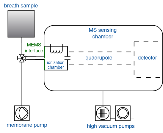
Figure 1: A schematic representation of the experimental apparatus.

This device allows to reduce the inlet gas flow by more than four orders of magnitude, with respect to standard MS gas analizers, and is able to operate with ultra-simplified vacuum systems Franceschelli et al. (2023). Furthermore, this new technology allows to sample at constant pressure instead of constant flux, removing the need for additional tools for flux control Franceschelli et al. (2023).

Such devices allow to optimize sensitivity and to reduce measurement time, thus providing an ideal tool for several applications, including diagnosis through breath analysis. By studying the mass spectrum, it is possible to obtain information about the chemical composition of the breath, including the presence of various VOCs.

3.2 Pre-processing

Once the obtained dataset composed by the acquisitions of the spectra for each patient has been stored, signals are cleaned through a pre-processing procedure that reduces noise and machine-variation of the acquisitions.

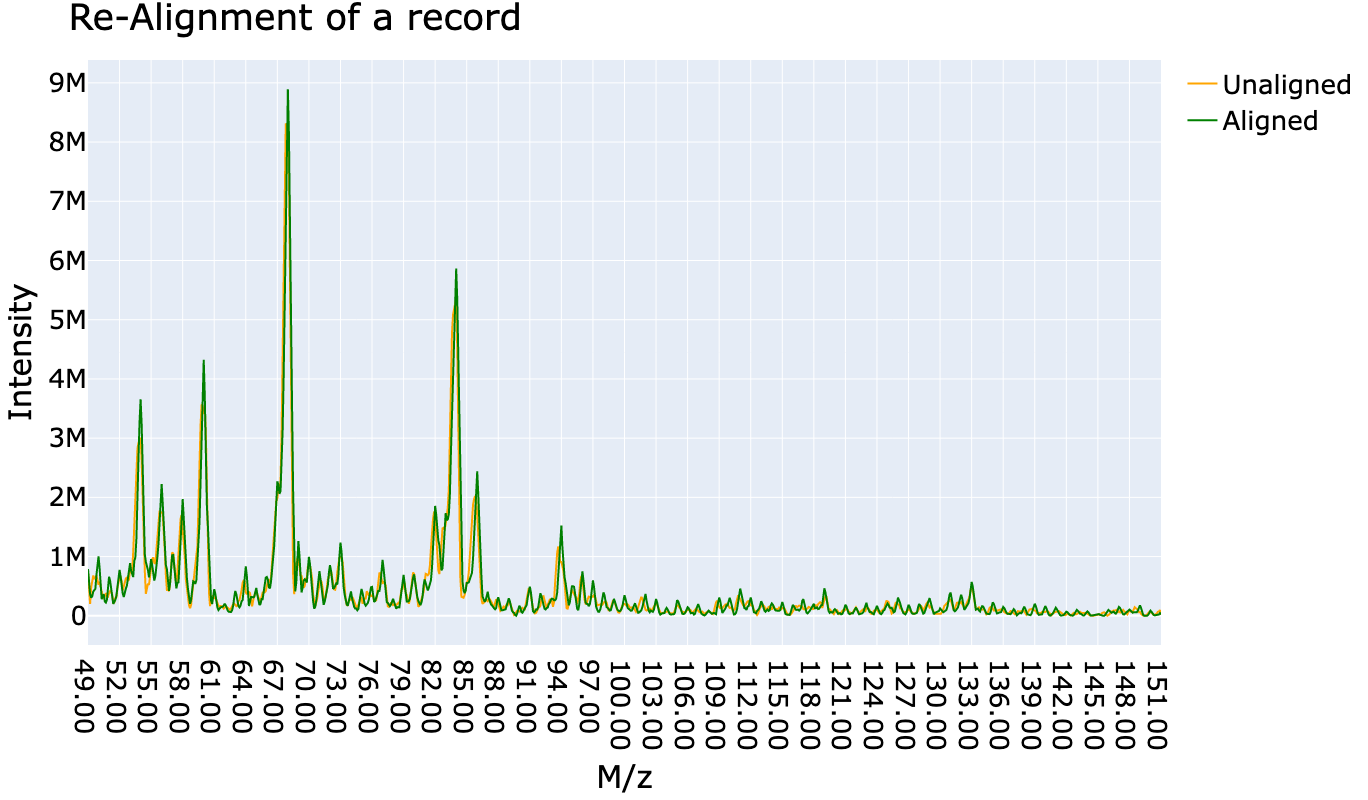
Figure 3: Aligned and non-aligned peaks of the mass spectrum of a single patient.

For each acquisition, the recorded m/z positions may be shifted with a specific alignment when the machine records the quantity of the ionized molecules due to measurement noise. A peak-alignment procedure is thus necessary. This procedure enables reducing the noise of the machine and compacting information. The peak alignment procedure is based on moving the peak to the nearest integer position, using them as anchors. The curves between two nearby peaks are stretched or compressed to sustain their original shape, preventing information loss. Peaks with mass $i$ are thus moved to the nearest integer position. Stretching and compression between peaks is done by linear interpolation to fit the corresponding segments in the reference. A graphical plot after the peak alignment can be seen in fig. 3. By summing all the intensities for each m/z in each acquisition, we can obtain the Total Ion Current (TIC) curve plot in fig. 2. After a certain time, the TIC curve stabilizes, reaching a plateau.

For each patient, we can obtain a single robust mass-spectra measurement by averaging the acquisitions in the plateau zone. To achieve this, first, it is necessary to identify the plateau in the TIC curve by means of gradient computation of the signal. A plateau-searching procedure was implemented, based on looking for acquisitions that do not vary so much from each other. The plateau searching procedure was implemented as follows:

• For each acquisition, we first applied a 1D-uniform filter to smooth the signals. This is based on taking the arithmetic average of each mass intensity value with its neighbors, with a window size of 1.

• We computed the gradient of the signals.

• A plateau is a zone that is almost flat, ideally where the gradient is zero, or in which the gradient does not vary so much from zero: we computed a tolerance guard-band $\epsilon$, to identify as “flat” a zone in which the gradient is near to zero (i. e., its absolute value is below $\epsilon$). This $\epsilon$ was computed on the basis of the $q-th$ quantile, in which $q$ is a number in the range $[0,1]$ that indicates how tolerant the requirement of the constant slope of the plateau is.

• Once the plateau of maximum length is found (that vary from 3 to 5 acquisition, for each patient), we computed standard deviations of acquisition in the plateau by deploying a rolling window of size 4. We then found the acquisitions for which the rolling window of standard deviation is minimum, and we computed the mean among these acquisitions, obtaining a single spectrum for each patient.

The model is trained on all the acquisitions extracted in the plateau zone by the procedure described above. This permits increasing both the number of training samples by a factor of 3-4 and the variability in the data, thus, leading to more accurate models. During the testing phase, instead, we considered a single mass spectrum for each patient, extracted by averaging the multiple acquisitions of each patient.

To eliminate both noise in the measurements and the possible parameters variations in the setting of the machine on different days, a signal smoothing procedure was implemented. We first normalized each spectra by dividing for the TIC, in order to obtain relative information about the breath composition (i. e., each intensity was divided by the sum of all the intensities, thus scaling the feature in the range $(0,1)$). We then applied a high-pass filter, considering as noise (and thus, treating as zero) each intensity below $0.0001$. Then, we applied a Savitzky-Golay Smoothing and Differentiation Filter Gallagher (2020); Savitzky and Golay (1964) to remove noise and align the signals to the baseline. This type of filter is used as a pre-processing step in spectra analysis to reduce both high-frequency noises, due to its smoothing properties, and low-frequency signals using differentiation. We then applied again a high-pass filter, considering as zero each intensity below $0.001$, to remove possible artifacts introduced by the filtering procedure.

Once implemented the filtering and pre-processing procedure for a single mass range, we applied it to all the mass ranges and combined the obtained spectra. Since we consider different acquisitions for each mass range, merging them together means considering all the combinations of the different acquisitions for each range. In other words, the expansion lead to a dataset in which each row is a particular combination of the different acquisition of each mass range, for each patient. This procedure is something similar to creating artificial rows-patients, in which each of them varies for one of the four pieces of the spectra. As an additional step, we further normalized the whole spectra by the total sum of the intensity, obtaining only relative information in the range $(0,1)$.

3.3 Machine-Learning Models

Several machine-learning (ML) techniques have been used by scholars in the context of COVID-19 Costa et al. (2022); Smolinska et al. (2014). We propose to exploit state-of-the-art ML models: K-nearest neighbors (KNN) random forest (RF), logistic regression (LR), gradient boosting (XB), support vector machine (SVM) with RBF kernel, and an ensemble made by all the model together, in a hard-voting fashion (Ens). To reduce the feature that ML models should analyze, simplify the model, and avoid overfitting, feature reduction techniques are used.

Features are filtered by removing all the feature that present a variance equal to zero (thus, we removed all the m/z for which no intensities were measured in the filtered dataset). Then they are normalized by means of standard normalization approaches (Standard Scaler). The Standard Scaler scales each feature by subtracting the mean and diving by the variance. However, the outliers have an influence when computing the empirical mean and standard deviation. Therefore, it may not ensure a balanced scaling of features in the presence of outliers. To solve this issue, we propose to use a Robust Scaler: the centering and scaling statistics computed by this type of normalization approach are based on percentiles and are therefore not influenced by a few very large marginal outliers. This removes the median and scales the data according to the interquartile range (the IQR), which is the range between the 1 quartile (25 percentile) and the 3 quartile (75 percentile).

Then, we used principal component analysis (PCA) Gao et al. (2020); Jolliffe (2002) to extract the first 20 principal components of our dataset. But before applying the PCA, a further step of feature selection approach can be performed, to select only the most informative features, the ones the most linked to the target task (in a supervised-feature selection fashion).

For this purpose, we used a Relief based algorithm Kira and Rendell (1992), called SURF*. Relief algorithm use a filter-method approach to feature selection that is notably sensitive to feature interactions. It is based on having a feature score. The scoring involves comparing feature values between pairs of neighboring instances to determine their importance. If a feature value difference is detected in a neighboring instance pair with the same class, the feature score is decreased, which is known as a hit. On the other hand, if a feature value difference is observed in a neighboring instance pair with different class values, the feature score is increased, which is referred to as a miss.

The SURF algorithm is a variant of the Relief algorithm that considers nearest neighbors, including both hits and misses, based on a distance threshold from the target instance. The distance threshold is defined by the average distance between all pairs of instances in the training data. According to research Greene et al. (2009), SURF has been found to outperform ReliefF in detecting 2-way interactions. SURF* (or SURF Star) Greene et al. (2010) is an extension of the SURF algorithm that not only considers near neighbors but also far instances in the scoring updates. However, inverted scoring updates are employed for far instance pairs.

3.4 Model Evaluation

Patients have been split into training and test data: the training data are used to create the ML models, while the testing data are used only for evaluation purposes. We evaluated the experiments on 10 different training-test splits, averaging the results to obtain an unbiased estimation of the generalization performances of our models. We used a 10-fold Stratified Cross Validation. Results are presented in terms of famous classification performances: balanced accuracy ($A$), precision ($P$), recall ($R$), and F1-Score ($F1$).

These metrics are computed on the basis of the number of samples correctly and incorrectly predicted by our model and are based on the concept of true positives, true negatives, false positives, and false negatives. A true positive ($TP$) is an outcome where the model correctly predicts the positive class. Similarly, a true negative ($TN$) is an outcome where the model correctly predicts the negative class. A false positive ($FP$) is an outcome where the model incorrectly predicts the positive class. And a false negative FN is an outcome where the model incorrectly predicts the negative class. The balanced accuracy avoids inflated performance estimates on imbalanced datasets. It is the macro-average of recall scores. Intuitively, the precision is the ability of the classifier not to label as positive a sample that is negative, while recall is the ability of the classifier to find all the positive samples. The F1 score can be interpreted as a harmonic mean of the precision and recall, where an $F1$ score reaches its best value at 1 and worst score at 0. The relative contribution of precision and recall to the $F1$ score are equal. In formula, $A$, $P$, $R$, and $F1$ are computed as below:

$$A=\frac{1}{2}\left(\frac{TP}{TP+FN}+\frac{TN}{TN+FP}\right)$$ (1)

$$P=\frac{TP}{TP+FP}$$ (2)

$$R=\frac{TP}{TP+FN}$$ (3)

$$F1=2\frac{P\cdot R}{P+R}$$ (4)

For experiments on the whole mass spectra with the four ranges together, we also computed two additional performance metrics, that are Specificity and the area under the receiver operating characteristic curve (ROC-AUC). While the recall is a measure that evaluates a test’s ability to correctly identify unhealthy individuals without a particular condition, specificity carry the same concept but for the healthy patients. It is calculated using the formula $specificity=\frac{TN}{TN+FP}$ Essentially, specificity represents the probability of obtaining a negative test result when a patient is actually healthy. When a test exhibits high specificity, a positive result becomes valuable in confirming the presence of the disease, as the test rarely produces positive outcomes in healthy individuals. If a test has 100% specificity, it will correctly identify all patients without the disease by yielding negative results. Thus, a positive test outcome would definitively indicate the presence of the disease. Another way to interpret specificity is as the recall of the negative class.

A receiver operating characteristic (ROC) curve is a visual representation that showcases the performance of a binary classifier system as the threshold for classification is adjusted. It plots the true positive rate (TPR) against the false positive rate (FPR) at different threshold values. TPR is also referred to as sensitivity, while FPR is the complement of specificity.

The ROC-AUC quantifies the overall performance of the classifier by calculating the area beneath the ROC curve. This single numerical value summarizes the information conveyed by the entire curve.

4 Experimental Evaluation

Breath samples were collected from patients and medical personnel at Varese Hospital (Ospedale di Circolo — Fondazione Macchi, ASST Sette Laghi). The acquisition lasted complexively one year, from March 2021 to March 2022, for a total of 302 tested subjects, some tested more than once to calibrate the system. The mass spectra have been collected with a Varian 1200L mass analyzer, combined with the MEMS interface, as shown in Figure 1. As ground truth to confirm SARS-CoV-2 infection, a RT-qPCR nasopharyngeal swab testing has been performed on all subjects.

4.1 Test protocol

The subject’s breath is collected into a sampling tedlar bag with a defined volume of 3 litres, by having the subject blow through a straw directly into the bag. Then, the bag is connected to the inlet valve of the MS apparatus.

As shown in Fig. 1, the inlet valve can have two possible settings: the first setting allows for the sample mixture, at atmospheric pressure, to flow from the bag to the ionization chamber, directly through the MEMS interface; the second setting connects the MEMS interface to a membrane pump, in order to clean the inlet line, bringing it to vacuum conditions ($\simeq\qty{1e-3}{\milli\bar{}}$). Figure 2 shows the TIC behaviour when the breath sample flows into the MS system: the initial increase is due to the abrupt pressure change at the valve opening and, after a few tens of second, TIC curve shows a plateau regionBagolini et al. (2021) when the flux reaches stability.

Mass spectra are recorded via the Varian 1200L mass analyzer software, which allows to set some acquisition parameters like mass range, acquisition time and electron multiplier (EM) voltage. The latter parameter ultimately sets the detector amplification factor.

We recorded mass spectra in the following ranges:

• 1051m/z, with an acquisition time of 10s and EM voltage of 1000V;

• 49151m/z, with an acquisition time of 14s and EM voltage of 1800V;

• 149251m/z, with an acquisition time of 14s and EM voltage of 1800V;

• 249351m/z, with an acquisition time of 14s and EM voltage of 1800V;

To avoid signal saturation, the amplification in the first mass range was reduced due to the presence of the most abundant breath components, namely $\text{CO}_{2}$ (44m/z), $\text{N}_{2}$ (28m/z) and $\text{O}_{2}$ (32m/z).

Figure 2: Total Ion Current (TIC) of a recording from one sample. The recording is made up of about 10 acquisitions (green dots), each corresponding to a mass spectrum. The spectra used for the analysis are selected on the plateau of TIC (red dotted region).

4.2 Data Analysis

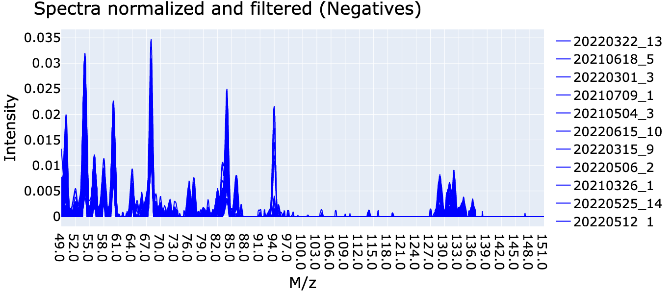
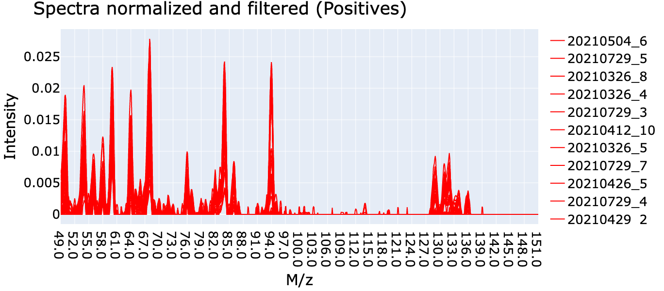
Figure 4: The comparison of spectra before (top) and after the filtering and normalizing procedure (bottom) shows the removal of low-frequency noise. Negative patients are on the left (blue), positive on the right (red).

The raw dataset presents breath samples for a total of $1208$ acquisitions in 302 patients, divided into 91 positive records and 211 negative records. After removing outliers (with a $z$-score greater than 8, for at least one feature) and patient for which it was not possible to identify a plateau, we reached 287 patients for mass range 2 and 203 if we consider all the ranges. These problems were caused by the highly prototypical nature of the equipment; it is worth noticing that, in a real application, it would have been possible to repeat the measurement. To address the issue of high class imbalance, we utilized a simple oversampling technique on the minority class (i. e., the COVID-19 positive class) in each iteration of the training-test procedure.

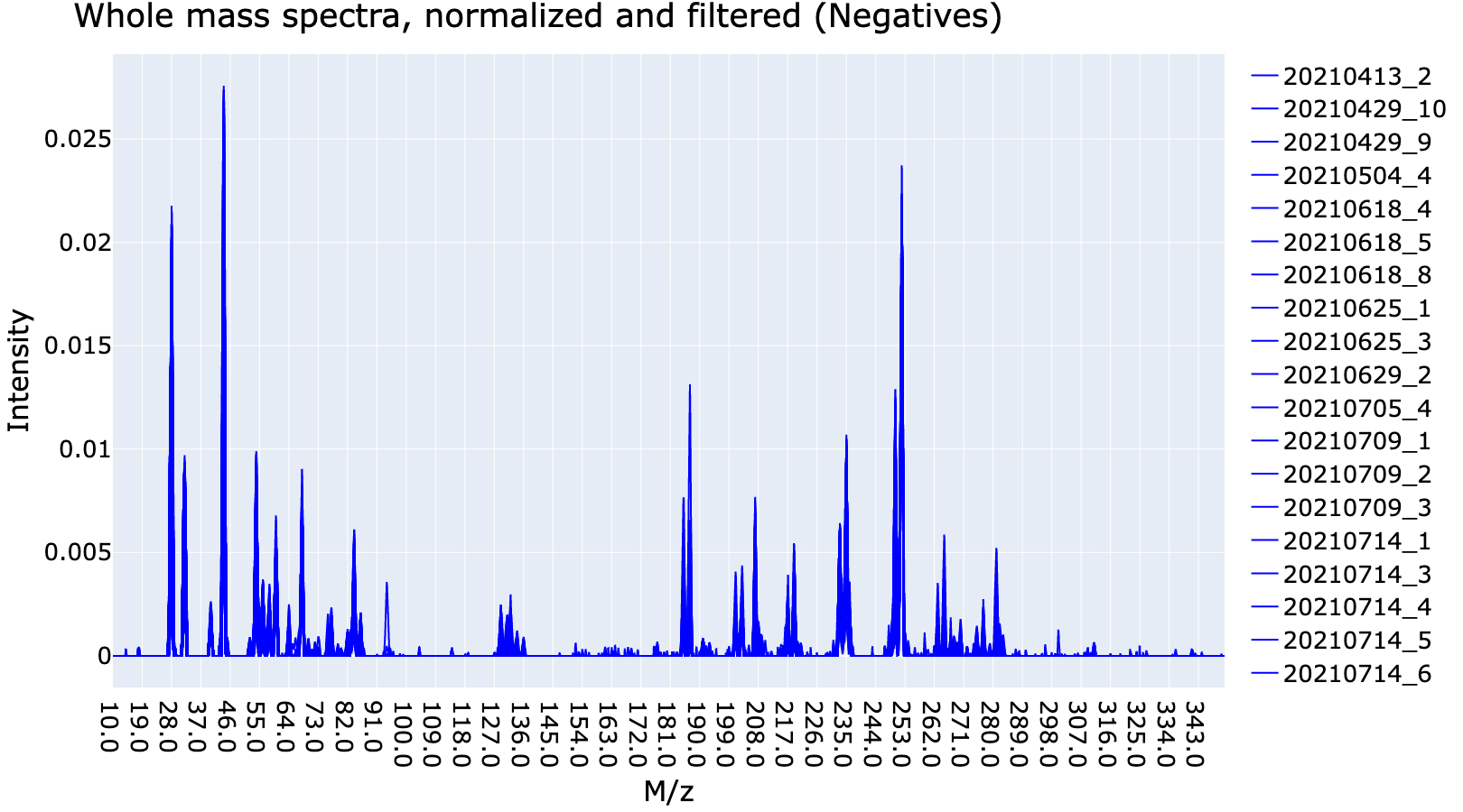
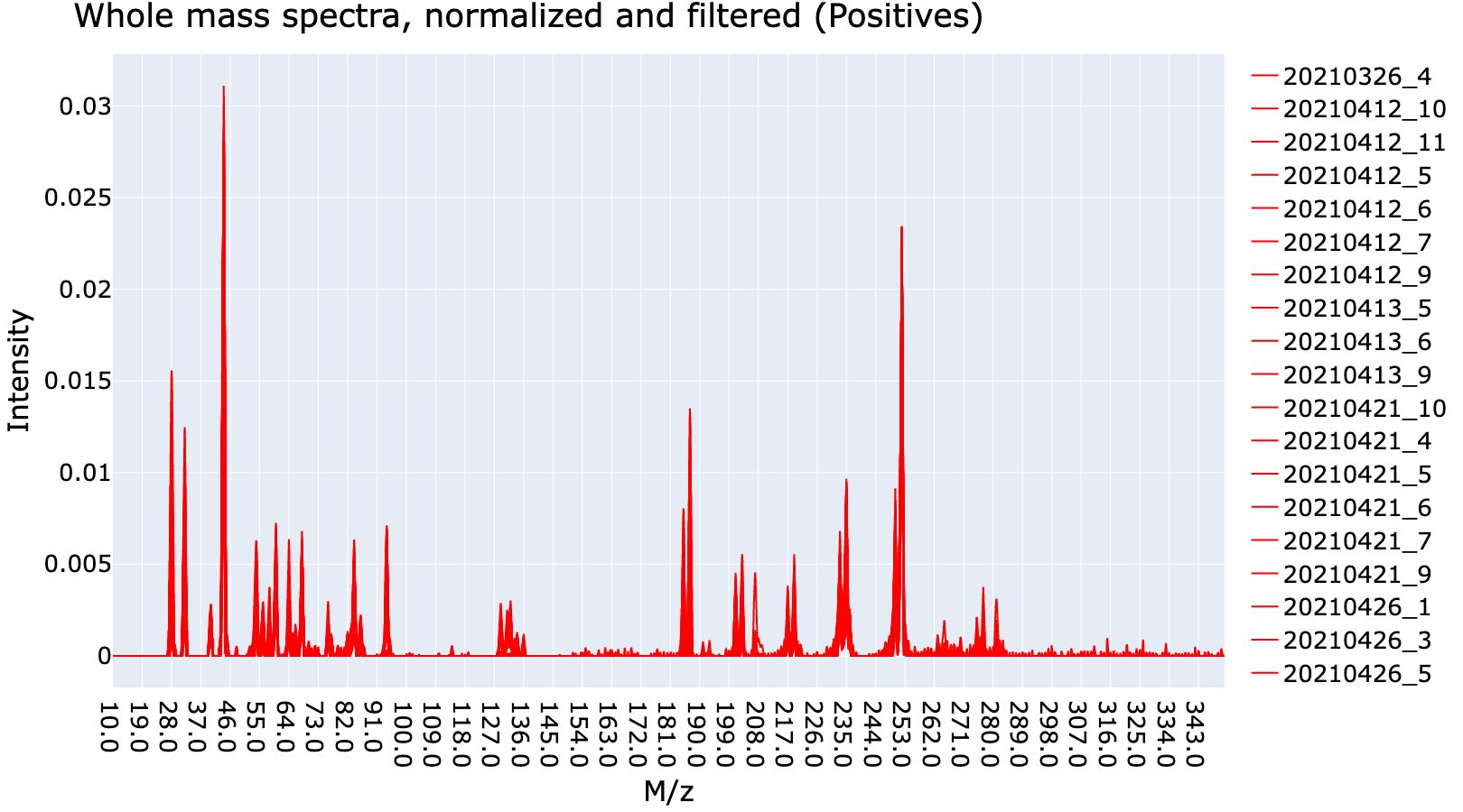
Figure 5: Examples of whole spectra (10351m/z) for negative subjects (top, blue) and positive ones (bottom, red)

The results of the approaches described in 3.2 can be found in table 2. The expansion procedure increased the dimensionality of the dataset to $47\ 084$ samples but created from only 203 patients. A graphical 2D representation of the points obtained with t-SNE dimensionality reduction van der Maaten and Hinton (2008) is presented in figure fig. 6. There, a precise boundary between positive and negative samples can be seen.

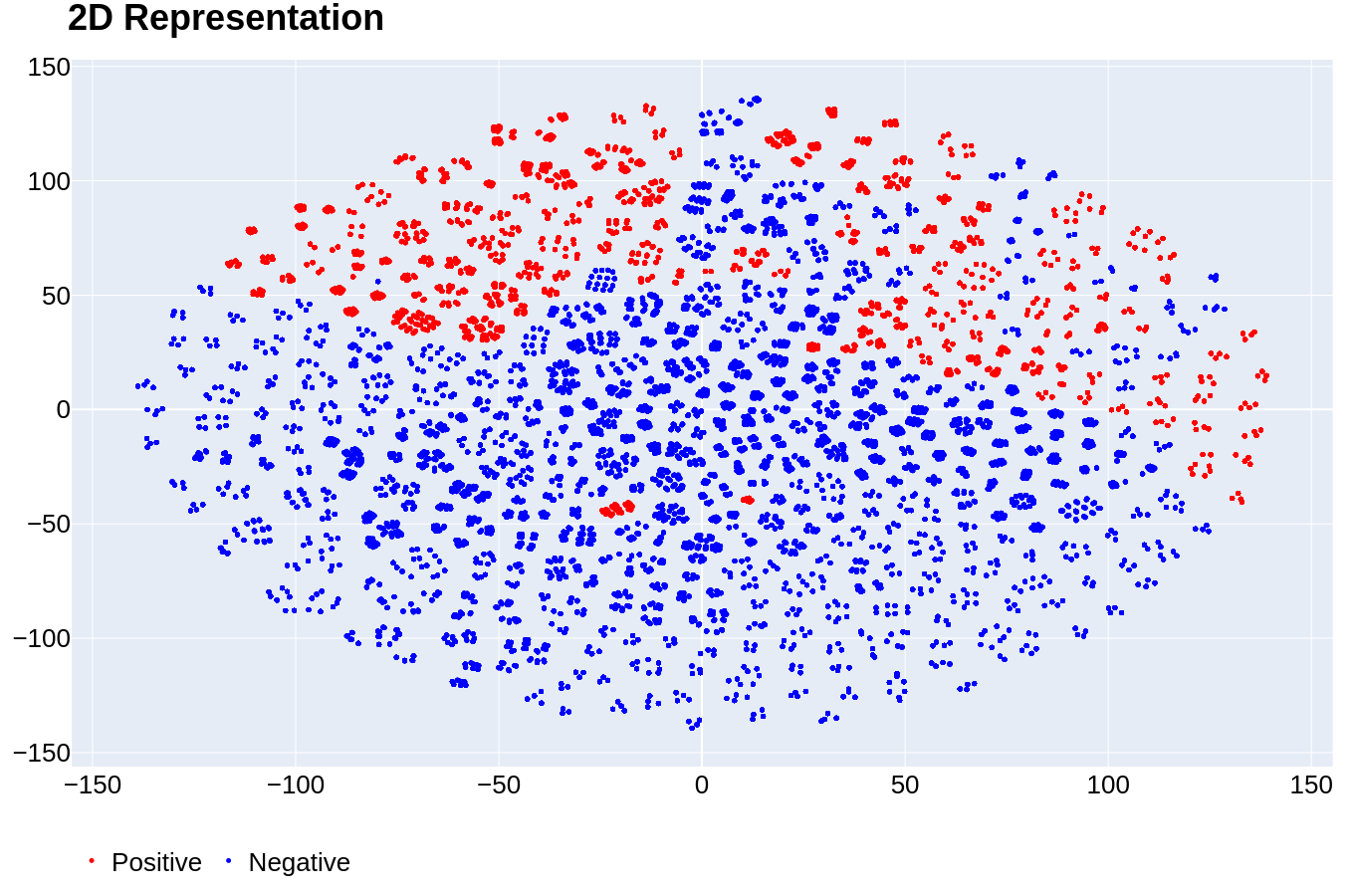
Figure 6: 2D t-SNE representation of the whole spectra for all the 47,084 samples generated.

The filtering of features reduced the number of features from $1021$ to $611$ in the mass range 2 and from $3411$ to $1734$ in the whole spectrum. The results of training on different mass ranges and testing them on the test sets without feature pre-processing seems to indicate mass range 2 as the more useful for classification with a F1 score of 0.70 and accuracy of 0.83 (tables 1 and 2).

As shown in table 2, the idea of inserting multiple acquisition for each patient in the training set, while averaging them on the test set, lead to a lower prediction error and higher classification performance with respect to a single, robust spectrum. With the Ensemble model, we can reach the 91.4% of balanced accuracy and the 86.9% of F1-Score if we include all the stable acquisitions in the training set, while we reached the 89.8% of accuracy and 84.8 % of F1-Score with the same ensemble model, but with a single acquisition per patient. This hold also for the other model taken into account. Filtering and normalizing the spectra is also beneficial, since it permits to increase the classification performance for all the models: if we compare table 1 and table 2, it is evident that, for range 2, we increased the accuracy from 84% to 93.4%, and the F1-Score from 70% to about 89%.

The SVC and Ensemble algorithms have the highest recall values for all the data processing setup, indicating that they have the highest ability to correctly identify true positives patients. In general, these two algorithms have the highest prediction performances, that, in principle, could be additionally improved with a fine search in the hyperparameters.

Including a Feature Selection steps was not beneficial in terms of error metrics: with the SURF* algorithm, the error metrics decrease. It may be due to complex interaction between features, that this algorithm is not able to catch. The robust scaler permits to decrease the standard deviation in the performance metrics, and thus the error fluctuations, due to the ability to deal with outliers values. It is extremely beneficial in the case of SVM, and also with the Ensemble method.

Using all the spectra together, and the subsequent artificial samples creation technique permitted used to reach the best performances in terms of error metric table 3: with the ensemble method, we achieve 95% accuracy, 94% recall, 96% specificity, and F1-score of 92%.

Table 1: Average results with different mass ranges on the test set on 10 runs, no features pre-processing

Model	Mass Range	Accuracy	Precision	Recall	F1-Score
RF	1	0.78	0.65	0.56	0.60
RF	2	0.82	0.69	0.69	0.68
RF	3	0.82	0.72	0.57	0.63
RF	4	0.79	0.65	0.53	0.57
Ens	1	0.82	0.70	0.67	0.68
Ens	2	0.84	0.75	0.69	0.71
Ens	3	0.80	0.68	0.57	0.61
Ens	4	0.77	0.62	0.60	0.59

Table 2: Mean Results of Classification Algorithms on the test sets with mass range 2

Alg.	Filtering	Feat. Sel.	Acquisition	Accuracy	Precision	Recall	F1 Score
xGB	No	PCA	Single	0.83 $\pm$ 0.04	0.74 $\pm$ 0.10	0.77 $\pm$ 0.08	0.75 $\pm$ 0.06
xGB	Yes	PCA	Single	0.88 $\pm$ 0.07	0.79 $\pm$ 0.08	0.86 $\pm$ 0.13	0.82 $\pm$ 0.09
xGB	Yes	PCA	Multiple	0.93 $\pm$ 0.05	0.85 $\pm$ 0.14	0.94 $\pm$ 0.07	0.88 $\pm$ 0.09
xGB	Yes	SURF*, PCA	Multiple	0.86 $\pm$ 0.07	0.78 $\pm$ 0.14	0.83 $\pm$ 0.10	0.80 $\pm$ 0.10
xGB	Yes (RS)	PCA	Multiple	0.90 $\pm$ 0.04	0.82 $\pm$ 0.10	0.89 $\pm$ 0.08	0.84 $\pm$ 0.05
KNN	No	PCA	Single	0.89 $\pm$ 0.05	0.73 $\pm$ 0.09	0.92 $\pm$ 0.08	0.81 $\pm$ 0.07
KNN	Yes	PCA	Single	0.87 $\pm$ 0.05	0.73 $\pm$ 0.07	0.89 $\pm$ 0.08	0.80 $\pm$ 0.07
KNN	Yes	PCA	Multiple	0.91 $\pm$ 0.07	0.80 $\pm$ 0.14	0.93 $\pm$ 0.10	0.85 $\pm$ 0.11
KNN	Yes	SURF*, PCA	Multiple	0.85 $\pm$ 0.07	0.70 $\pm$ 0.13	0.87 $\pm$ 0.10	0.77 $\pm$ 0.11
KNN	Yes (RS)	PCA	Multiple	0.91 $\pm$ 0.05	0.78 $\pm$ 0.12	0.94 $\pm$ 0.08	0.84 $\pm$ 0.08
LR	No	PCA	Single	0.86 $\pm$ 0.05	0.71 $\pm$ 0.12	0.88 $\pm$ 0.07	0.78 $\pm$ 0.08
LR	Yes	PCA	Single	0.85 $\pm$ 0.06	0.71 $\pm$ 0.08	0.85 $\pm$ 0.10	0.77 $\pm$ 0.07
LR	Yes	PCA	Multiple	0.88 $\pm$ 0.06	0.73 $\pm$ 0.14	0.92 $\pm$ 0.10	0.80 $\pm$ 0.10
LR	Yes	SURF*, PCA	Multiple	0.88 $\pm$ 0.07	0.74 $\pm$ 0.13	0.89 $\pm$ 0.10	0.80 $\pm$ 0.10
LR	Yes (RS)	PCA	Multiple	0.89 $\pm$ 0.05	0.76 $\pm$ 0.11	0.91 $\pm$ 0.08	0.82 $\pm$ 0.08
RF	No	PCA	Single	0.87 $\pm$ 0.05	0.79 $\pm$ 0.10	0.84 $\pm$ 0.09	0.81 $\pm$ 0.07
RF	Yes	PCA	Single	0.89 $\pm$ 0.04	0.82 $\pm$ 0.11	0.87 $\pm$ 0.08	0.84 $\pm$ 0.05
RF	Yes	PCA	Multiple	0.91 $\pm$ 0.07	0.80 $\pm$ 0.14	0.92 $\pm$ 0.09	0.85 $\pm$ 0.10
RF	Yes	SURF*, PCA	Multiple	0.85 $\pm$ 0.09	0.75 $\pm$ 0.16	0.82 $\pm$ 0.13	0.78 $\pm$ 0.12
RF	Yes (RS)	PCA	Multiple	0.90 $\pm$ 0.03	0.81 $\pm$ 0.07	0.90 $\pm$ 0.07	0.84 $\pm$ 0.04
SVC	No	PCA	Single	0.65 $\pm$ 0.07	0.82 $\pm$ 0.20	0.32 $\pm$ 0.13	0.45 $\pm$ 0.16
SVC	Yes	PCA	Single	0.76 $\pm$ 0.10	0.82 $\pm$ 0.15	0.57 $\pm$ 0.17	0.66 $\pm$ 0.15
SVC	Yes	PCA	Multiple	0.89 $\pm$ 0.05	0.76 $\pm$ 0.13	0.91 $\pm$ 0.13	0.81 $\pm$ 0.07
SVC	Yes	SURF*, PCA	Multiple	0.86 $\pm$ 0.08	0.77 $\pm$ 0.17	0.83 $\pm$ 0.09	0.79 $\pm$ 0.12
SVC	Yes (RS)	PCA	Multiple	0.93 $\pm$ 0.04	0.85 $\pm$ 0.09	0.94 $\pm$ 0.07	0.89 $\pm$ 0.06
Ens.	No	PCA	Single	0.87 $\pm$ 0.03	0.77 $\pm$ 0.10	0.84 $\pm$ 0.06	0.80 $\pm$ 0.06
Ens.	Yes	PCA	Single	0.90 $\pm$ 0.07	0.82 $\pm$ 0.11	0.89 $\pm$ 0.10	0.85 $\pm$ 0.09
Ens.	Yes	PCA	Multiple	0.93 $\pm$ 0.07	0.83 $\pm$ 0.15	0.94 $\pm$ 0.09	0.87 $\pm$ 0.11
Ens.	Yes	SURF*, PCA	Multiple	0.89 $\pm$ 0.07	0.79 $\pm$ 0.16	0.88 $\pm$ 0.08	0.82 $\pm$ 0.12
Ens.	Yes (RS)	PCA	Multiple	0.92 $\pm$ 0.04	0.81 $\pm$ 0.09	0.94 $\pm$ 0.07	0.87 $\pm$ 0.06

Table 3: Mean Results (10 Splits) for the whole mass range 10-351.

Alg.	Accuracy	Precision	Recall	F1 Score	Specificity	ROC-AUC
KNN	0.93 $\pm$ 0.06	0.87 $\pm$ 0.09	0.92 $\pm$ 0.09	0.89 $\pm$ 0.08	0.94 $\pm$ 0.04	0.95 $\pm$ 0.04
RF	0.91 $\pm$ 0.06	0.88 $\pm$ 0.10	0.87 $\pm$ 0.12	0.87 $\pm$ 0.07	0.95 $\pm$ 0.04	0.98 $\pm$ 0.03
LR	0.94 $\pm$ 0.04	0.84 $\pm$ 0.12	0.96 $\pm$ 0.07	0.89 $\pm$ 0.07	0.93 $\pm$ 0.05	0.97 $\pm$ 0.04
xGB	0.94 $\pm$ 0.03	0.88 $\pm$ 0.08	0.93 $\pm$ 0.07	0.90 $\pm$ 0.03	0.95 $\pm$ 0.03	0.98 $\pm$ 0.03
SVC	0.93 $\pm$ 0.06	0.89 $\pm$ 0.09	0.90 $\pm$ 0.12	0.88 $\pm$ 0.06	0.95 $\pm$ 0.04	0.98 $\pm$ 0.02
Ens.	0.95 $\pm$ 0.04	0.90 $\pm$ 0.08	0.94 $\pm$ 0.07	0.92 $\pm$ 0.05	0.96 $\pm$ 0.03	0.98 $\pm$ 0.03

5 Conclusions

We presented a framework for COVID-19 detection by breath samples. We used a prototype of a special MS portable machine able based on nanotechnology to analyze human breath in about 2 minutes, extracting the mass spectrum of a patient in the interval 10-351, divided into four sub-ranges. Experiments showed that the mass spectra can be related to the presence of COVID-19 by means of ML classification models. We proposed a filtering procedure based on Savitzky-Golay filter to reduce possible noise in the acquisitions. Results showed that with simple approaches we are able to get about 93% accuracy and 94% recall with mass range of 49151m/z, which seems to be the most appropriate in predicting COVID-19 disease. We found out that the use of Robust scaling techniques, based on the median and IQR scaling, in conjunction with PCA feature extraction were beneficial in predicting COVID-19 diseases. We were able to merge all the spectra ranges, reaching classification performances of about 95% of accuracy and 98% of ROC-AUC score. In general, the special portable MS machine is potentially deployable in COVID-19 hubs to detect in a fast, easy, comfortable way the presence or not of COVID-19. The use of ML to relate mass spectra to special diseases enables early detection, rapid test results, and less risk of infection for healthcare providers.

References

- Chu et al. [2020] Derek K Chu, Elie A Akl, Stephanie Duda, Karla Solo, Sally Yaacoub, Holger J Schünemann, Amena El-harakeh, Antonio Bognanni, Tamara Lotfi, Mark Loeb, Anisa Hajizadeh, Anna Bak, Ariel Izcovich, Carlos A Cuello-Garcia, Chen Chen, David J Harris, Ewa Borowiack, Fatimah Chamseddine, Finn Schünemann, Gian Paolo Morgano, Giovanna E U Muti Schünemann, Guang Chen, Hong Zhao, Ignacio Neumann, Jeffrey Chan, Joanne Khabsa, Layal Hneiny, Leila Harrison, Maureen Smith, Nesrine Rizk, Paolo Giorgi Rossi, Pierre AbiHanna, Rayane El-khoury, Rosa Stalteri, Tejan Baldeh, Thomas Piggott, Yuan Zhang, Zahra Saad, Assem Khamis, and Marge Reinap. Physical distancing, face masks, and eye protection to prevent person-to-person transmission of SARS-CoV-2 and COVID-19: a systematic review and meta-analysis. Lancet (London, England), 395(10242):1973–1987, Jun 2020. ISSN 1474-547X. doi:10.1016/S0140-6736(20)31142-9.
- Vandenberg et al. [2021] Olivier Vandenberg, Delphine Martiny, Olivier Rochas, Alex van Belkum, and Zisis Kozlakidis. Considerations for diagnostic COVID-19 tests. Nature Reviews Microbiology, 19(3):171–183, Mar 2021. ISSN 1740-1526, 1740-1534. doi:10.1038/s41579-020-00461-z.
- Feng et al. [2020] Wei Feng, Ashley M. Newbigging, Connie Le, Bo Pang, Hanyong Peng, Yiren Cao, Jinjun Wu, Ghulam Abbas, Jin Song, Dian-Bing Wang, Mengmeng Cui, Jeffrey Tao, D. Lorne Tyrrell, Xian-En Zhang, Hongquan Zhang, and X. Chris Le. Molecular diagnosis of COVID-19: Challenges and research needs. Analytical Chemistry, 92(15):10196–10209, Aug 2020. ISSN 1520-6882. doi:10.1021/acs.analchem.0c02060.
- Eissa and Zourob [2021] Shimaa Eissa and Mohammed Zourob. Development of a low-cost cotton-tipped electrochemical immunosensor for the detection of SARS-CoV-2. Analytical Chemistry, 93(3):1826–1833, Jan 2021. ISSN 0003-2700, 1520-6882. doi:10.1021/acs.analchem.0c04719.
- Wong and Medrano [2005] Marisa L. Wong and Juan F. Medrano. Real-time PCR for mRNA quantitation. BioTechniques, 39(1):75–85, 2005. doi:10.2144/05391RV01. PMID: 16060372.
- Bahreini et al. [2020] Fatemeh Bahreini, Rezvan Najafi, Razieh Amini, Salman Khazaei, and Saeid Bashirian. Reducing false negative PCR test for COVID-19. International Journal of Maternal and Child Health and AIDS (IJMA), 9(3):408–410, Oct 2020. ISSN 2161-864X, 2161-8674. doi:10.21106/ijma.421.
- Wang et al. [2020] Kaijin Wang, Xuetong Zhu, and Jiancheng Xu. Laboratory biosafety considerations of SARS-CoV-2 at biosafety level 2. Health Security, 18(3):232–236, Jun 2020. ISSN 2326-5094, 2326-5108. doi:10.1089/hs.2020.0021.
- Lamote et al. [2020] Kevin Lamote, Eline Janssens, Eline Schillebeeckx, Therese S Lapperre, Benedicte Y De Winter, and Jan P van Meerbeeck. The scent of COVID-19: viral (semi-)volatiles as fast diagnostic biomarkers? Journal of Breath Research, 14(4):042001, Jul 2020. ISSN 1752-7163. doi:10.1088/1752-7163/aba105.
- Song et al. [2020] Jin-Wen Song, Sin Man Lam, Xing Fan, Wen-Jing Cao, Si-Yu Wang, He Tian, Gek Huey Chua, Chao Zhang, Fan-Ping Meng, Zhe Xu, Jun-Liang Fu, Lei Huang, Peng Xia, Tao Yang, Shaohua Zhang, Bowen Li, Tian-Jun Jiang, Raoxu Wang, Zehua Wang, Ming Shi, Ji-Yuan Zhang, Fu-Sheng Wang, and Guanghou Shui. Omics-driven systems interrogation of metabolic dysregulation in COVID-19 pathogenesis. Cell Metabolism, 32(2):188–202.e5, Aug 2020. ISSN 15504131. doi:10.1016/j.cmet.2020.06.016.
- Rattray et al. [2014] Nicholas J.W. Rattray, Zahra Hamrang, Drupad K. Trivedi, Royston Goodacre, and Stephen J. Fowler. Taking your breath away: metabolomics breathes life in to personalized medicine. Trends in Biotechnology, 32(10):538–548, 2014. ISSN 0167-7799. doi:https://doi.org/10.1016/j.tibtech.2014.08.003.
- Mansurova et al. [2018] M. Mansurova, Birgitta E. Ebert, Lars M. Blank, and Alfredo J. Ibáñez. A breath of information: the volatilome. Current Genetics, 64(4):959–964, Aug 2018. ISSN 0172-8083, 1432-0983. doi:10.1007/s00294-017-0800-x.
- Rodríguez-Aguilar et al. [2021] Maribel Rodríguez-Aguilar, Lorena Díaz de León-Martínez, Blanca Nohemí Zamora-Mendoza, Andreu Comas-García, Sandra Elizabeth Guerra Palomares, Christian Alberto García-Sepúlveda, Luz Eugenia Alcántara-Quintana, Fernando Díaz-Barriga, and Rogelio Flores-Ramírez. Comparative analysis of chemical breath-prints through olfactory technology for the discrimination between SARS-CoV-2 infected patients and controls. Clinica Chimica Acta, 519:126–132, Aug 2021. ISSN 00098981. doi:10.1016/j.cca.2021.04.015.
- Giovannini et al. [2021] Giorgia Giovannini, Hossam Haick, and Denis Garoli. Detecting COVID-19 from breath: A game changer for a big challenge. ACS sensors, 6(4):1408–1417, Apr 2021. ISSN 2379-3694. doi:10.1021/acssensors.1c00312.
- Rya [2021] Use of exhaled breath condensate (ebc) in the diagnosis of SARS-COV-2 (COVID-19). 76:86–88, Jan 2021. ISSN 0040-6376, 1468-3296. doi:10.1136/thoraxjnl-2020-215705.
- Smolinska et al. [2014] A. Smolinska, A. C. Hauschild, R. R. Fijten, J. W. Dallinga, J. Baumbach, and F. J. van Schooten. Current breathomics–a review on data pre-processing techniques and machine learning in metabolomics breath analysis. J Breath Res, 8(2):027105, Jun 2014. doi:10.1088/1752-7155/8/2/027105.
- Gasparri et al. [2016] Roberto Gasparri, Marco Santonico, Claudia Valentini, Giulia Sedda, Alessandro Borri, Francesco Petrella, Patrick Maisonneuve, Giorgio Pennazza, Arnaldo D’Amico, Corrado Di Natale, Roberto Paolesse, and Lorenzo Spaggiari. Volatile signature for the early diagnosis of lung cancer. Journal of Breath Research, 10(1):016007, Feb 2016. ISSN 1752-7163. doi:10.1088/1752-7155/10/1/016007.
- Janssens et al. [2020] Eline Janssens, Jan P. van Meerbeeck, and Kevin Lamote. Volatile organic compounds in human matrices as lung cancer biomarkers: a systematic review. Critical Reviews in Oncology/Hematology, 153:103037–, Sep 2020. ISSN 1879-0461. doi:10.1016/j.critrevonc.2020.103037.
- Oakley-Girvan and Davis [2017] Ingrid Oakley-Girvan and Sharon Watkins Davis. Breath based volatile organic compounds in the detection of breast, lung, and colorectal cancers: A systematic review. Cancer Biomarkers, 21(1):29–39, Dec 2017. ISSN 18758592, 15740153. doi:10.3233/CBM-170177.
- Behera et al. [2019] Bhagaban Behera, Rathin Joshi, G. K. Anil Vishnu, Sanjay Bhalerao, and Hardik J. Pandya. Electronic nose: a non-invasive technology for breath analysis of diabetes and lung cancer patients. Journal of Breath Research, 13(2):024001–, Mar 2019. ISSN 1752-7163. doi:10.1088/1752-7163/aafc77.
- Abd El Qader et al. [2015] Amir Abd El Qader, David Lieberman, Yonat Shemer Avni, Natali Svobodin, Tsilia Lazarovitch, Orli Sagi, and Yehuda Zeiri. Volatile organic compounds generated by cultures of bacteria and viruses associated with respiratory infections: Vocs generated by cultures of bacteria and viruses. Biomedical Chromatography, 29(12):1783–1790, Dec 2015. ISSN 02693879. doi:10.1002/bmc.3494.
- Mazzatenta et al. [2013] Andrea Mazzatenta, Camillo Di Giulio, and Mieczyslaw Pokorski. Pathologies currently identified by exhaled biomarkers. Respiratory Physiology & Neurobiology, 187(1):128–134, 2013. ISSN 1569-9048. doi:https://doi.org/10.1016/j.resp.2013.02.016. Immunopathology of the Respiratory System.
- de Lacy Costello et al. [2014] B. de Lacy Costello, A. Amann, H. Al-Kateb, C. Flynn, W. Filipiak, T. Khalid, D. Osborne, and N. M. Ratcliffe. A review of the volatiles from the healthy human body. Journal of Breath Research, 8(1):014001, Mar 2014. ISSN 1752-7163. doi:10.1088/1752-7155/8/1/014001.
- Hollywood et al. [2006] Katherine Hollywood, Daniel R. Brison, and Royston Goodacre. Metabolomics: Current technologies and future trends. PROTEOMICS, 6(17):4716–4723, 2006. doi:https://doi.org/10.1002/pmic.200600106.
- Davis et al. [2021] Cristina E. Davis, Michael Schivo, and Nicholas J. Kenyon. A breath of fresh air - the potential for COVID-19 breath diagnostics. EBioMedicine, 63:103183–, Jan 2021. ISSN 2352-3964. doi:10.1016/j.ebiom.2020.103183.
- Miekisch et al. [2004] Wolfram Miekisch, Jochen K. Schubert, and Gabriele F. E. Noeldge-Schomburg. Diagnostic potential of breath analysis–focus on volatile organic compounds. Clinica Chimica Acta; International Journal of Clinical Chemistry, 347(1–2):25–39, Sep 2004. ISSN 0009-8981. doi:10.1016/j.cccn.2004.04.023.
- Bruderer et al. [2019] Tobias Bruderer, Thomas Gaisl, Martin T. Gaugg, Nora Nowak, Bettina Streckenbach, Simona Müller, Alexander Moeller, Malcolm Kohler, and Renato Zenobi. On-line analysis of exhaled breath. Chemical Reviews, 119(19):10803–10828, Oct 2019. ISSN 0009-2665. doi:10.1021/acs.chemrev.9b00005.
- Berna et al. [2021] A. Z. Berna, E. H. Akaho, R. M. Harris, M. Congdon, E. Korn, S. Neher, M. M’Farrej, J. Burns, and A. R. Odom John. Reproducible breath metabolite changes in children with SARS-CoV-2 infection. ACS Infect Dis, 7(9):2596–2603, Sep 2021. doi:10.1101/2020.12.04.20230755.
- Zhang et al. [2022] Peize Zhang, Tantan Ren, Haibin Chen, Qingyun Li, Mengqi He, Yong Feng, Lei Wang, Ting Huang, Jing Yuan, Guofang Deng, and Hongzhou Lu. A feasibility study of COVID-19 detection using breath analysis by high-pressure photon ionization time-of-flight mass spectrometry. Journal of Breath Research, 16(4):046009, sep 2022. doi:10.1088/1752-7163/ac8ea1.
- Lima et al. [2022] Nerilson M. Lima, Bruno L. M. Fernandes, Guilherme F. Alves, Jéssica C. Q. de Souza, Marcelo M. Siqueira, Maria Patrícia do Nascimento, Olívia B. O. Moreira, Alessandra Sussulini, and Marcone A. L. de Oliveira. Mass spectrometry applied to diagnosis, prognosis, and therapeutic targets identification for the novel coronavirus SARS-CoV-2: A review. Analytica Chimica Acta, 1195:339385–, Feb 2022. ISSN 1873-4324. doi:10.1016/j.aca.2021.339385.
- Pratt and Prather [2012] Kerri A. Pratt and Kimberly A. Prather. Mass spectrometry of atmospheric aerosols—recent developments and applications. part ii: On-line mass spectrometry techniques. Mass Spectrometry Reviews, 31(1):17–48, 2012. doi:https://doi.org/10.1002/mas.20330.
- Aebersold and Mann [2003] Ruedi Aebersold and Matthias Mann. Mass spectrometry-based proteomics. Nature, 422(6928):198 – 207, 2003. doi:10.1038/nature01511.
- Dettmer et al. [2007] Katja Dettmer, Pavel A. Aronov, and Bruce D. Hammock. Mass spectrometry-based metabolomics. Mass Spectrometry Reviews, 26(1):51–78, 2007. doi:https://doi.org/10.1002/mas.20108.
- Dias et al. [2012] Daniel A. Dias, Sylvia Urban, and Ute Roessner. A historical overview of natural products in drug discovery. Metabolites, 2(2):303–336, 2012. ISSN 2218-1989. doi:10.3390/metabo2020303.
- Franceschelli et al. [2023] L. Franceschelli, C. Ciricugno, M. Di Lorenzo, A. Romani, A. Berardinelli, M. Tartagni, and R. Correale. Real-time gas mass spectroscopy by multivariate analysis. Scientific Reports, 13(1), 2023. doi:10.1038/s41598-023-33188-x.
- Mensa and Correale [2017a] Gianpiero Mensa and Raffaele Correale. Device for controlling a gaseous flow and systems and methods employing the device, May 2017a. URL https://patents.google.com/patent/US20170130870A1/en?oq=Patent+20170130870.
- Mensa and Correale [2017b] Gianpiero Mensa and Raffaele Correale. Portable electronic system for the analysis of time-variable gaseous flows, Jun 2017b. URL https://patents.google.com/patent/US20170168030A1/en?oq=Patent+20170168030.
- Mensa and Correale [2019] Gianpiero Mensa and Raffaele Correale. Portable electronic device for the analysis of a gaseous composition, Apr 2019. URL https://patents.google.com/patent/US10256084B2/en?oq=10256084.
- Bagolini et al. [2021] Alvise Bagolini, Raffaele Correale, Antonino Picciotto, Maurizio Di Lorenzo, and Marco Scapinello. Mems membranes with nanoscale holes for analytical applications. Membranes, 11(2), 2021. ISSN 2077-0375. doi:10.3390/membranes11020074.
- Roth [1990] A. Roth. Vacuum Technology. North Holland, 1990.
- Gallagher [2020] Neal Gallagher. Savitzky-golay smoothing and differentiation filter. 01 2020.
- Savitzky and Golay [1964] Abraham. Savitzky and M. J. E. Golay. Smoothing and differentiation of data by simplified least squares procedures. Analytical Chemistry, 36(8):1627–1639, Jul 1964. ISSN 0003-2700, 1520-6882. doi:10.1021/ac60214a047.
- Costa et al. [2022] Yandre M. G. Costa, Sergio A. Silva, Lucas O. Teixeira, Rodolfo M. Pereira, Diego Bertolini, Alceu S. Britto, Luiz S. Oliveira, and George D. C. Cavalcanti. COVID-19 detection on chest x-ray and ct scan: A review of the top-100 most cited papers. Sensors, 22(19), 2022. ISSN 1424-8220. doi:10.3390/s22197303.
- Gao et al. [2020] Zhihong Gao, Weifeng Zhang, Junjie Li, Jianhua Zhang, and Guangyan Huang. Principal component analysis-based feature selection for machine learning: A review. Expert Systems with Applications, 140:112920, 2020.
- Jolliffe [2002] Ian T Jolliffe. Principal component analysis, volume 2. Wiley Online Library, 2002.
- Kira and Rendell [1992] Kenji Kira and Larry A. Rendell. The feature selection problem: Traditional methods and a new algorithm. In Proceedings of the Tenth National Conference on Artificial Intelligence, AAAI’92, pages 129–134. AAAI Press, 1992. ISBN 0262510634.
- Greene et al. [2009] Casey S Greene, Nadia M Penrod, Jeff Kiralis, and Jason H Moore. Spatially uniform relieff (SURF) for computationally-efficient filtering of gene-gene interactions. BioData Min., 2(1):5, September 2009. doi:10.1186/1756-0381-2-5.
- Greene et al. [2010] Casey S. Greene, Daniel S. Himmelstein, Jeff Kiralis, and Jason H. Moore. The informative extremes: Using both nearest and farthest individuals can improve relief algorithms in the domain of human genetics. Lecture Notes in Computer Science, pages 182–193. Springer, 2010. ISBN 9783642122118.
- van der Maaten and Hinton [2008] Laurens van der Maaten and Geoffrey Hinton. Visualizing data using t-SNE. Journal of Machine Learning Research, 9(86):2579–2605, 2008. URL http://jmlr.org/papers/v9/vandermaaten08a.html.