The Global Fits of New Physics in $b\to s$ after $R_{K^{(*)}}$ 2022 Release

Abstract

The measurement of lepton universality parameters $R_{K^{(*)}}$ was updated by LHCb in December 2022, which indicated that the well-known anomalies in flavor-changing neutral current (FCNC) processes of B meson decays have faded away. However, does this mean that all new physics possibilities related to $b\to s\ell^{+}\ell^{-}$ have been excluded? We aim to answer this question in this work. The state-of-the-art effective Hamiltonian is adopted to describe $b\to s$ transition, while BSM (beyond the Standard Model) new physics effects are encoded in Wilson coefficients (WCs). Using around 200 observables in leptonic and semileptonic decays of B mesons and bottom baryons, measured by LHCb, CMS, ATLAS, Belle, and BaBar, we perform global fits of these Wilson coefficients in four different scenarios. In particular, lepton flavors in WCs are specified in some of the working scenarios. To see the change of new physics parameters, we use both the data before and after the 2022 release of $R_{K^{(*)}}$ in two separate sets of fits. We find that in three of the four scenarios, $\Delta C_{9}^{\mu}$ still has a deviation around or more than $4\sigma$ from the Standard Model. The lepton flavor in WCs is distinguishable for $\Delta C_{9}$ at the $1\sigma$ level, but at the $2\sigma$ level all the operators are flavor identical. We demonstrate numerically that there is no chirality for muon type of scalar operator and it is kept at the $1\sigma$ level for their electron type dual ones, while chiral difference exists for $\mathcal{O}_{9}^{\mu}$ at least at the $2\sigma$ level. Moreover, it can be deduced that the scalar operators $\mathcal{O}_{S,P}^{(^{\prime})\mu}$ become null if new physics emerges in terms of SMEFT (Standard Model Effective Field Theory) up to dimension-6.

I Introduction

The quest for new physics in FCNC process $b\to s\ell^{+}\ell^{-}$ has lasted for more than one decade. It was expected that in $B\to K^{*}\mu^{+}\mu^{-}$ new physics effect would emerge by measuring the forward-backward asymmetry (AFB), and the early measurements carried out by Belle [1], BaBar [2] and CDF [3] indeed seemed to prefer the new physics with a flipped $C_{7}$. In 2011, however, a SM-like behavior of AFB was confirmed by LHCb even with its $309\,\textrm{pb}^{-1}$ data [4]. Later on, more observables, including branching fractions, angular distributions and lepton universality parameters, were measured more and more precisely and deviations from SM predictions in particular bins were found by Belle [5, 6, 7], LHCb [8, 9, 10, 11, 12, 13, 14, 15, 16], ATLAS [17] and CMS [18, 19].

The non-universality of lepton flavor, characterized by $R_{K^{(*)}}\equiv\mathcal{B}({B}\to K^{(*)}\mu^{+}\mu^{-})/\mathcal{B}({B}\to K^{(*)}e^{+}e^{-})$, is among one of the anomalies appearing in semileptonic B meson decays. The $2.6\sigma$ deviation of $R_{K}$ in charged B meson decay was firstly reported in 2014 [8] and updated in 2019 [9] by LHCb. It was found by Belle in 2019 that a similar $2.6\sigma$ standard deviation also occurred at $q^{2}\in(1.0,6.0){\rm{GeV}}^{2}/c^{4}$ [6]. Later in 2021, with Run I and Run II dataset LHCb reported $R_{K}=0.846^{+0.042}_{-0.039}(\text{stat})^{+0.013}_{-0.012}(\text{sys})$ as well as $R_{K_{S}}=0.66^{+0.20}_{-0.14}(\text{stat})^{+0.02}_{-0.04}(\text{sys})$ at the level of $3.1\sigma$ and $1.4\sigma$, respectively. As for $B\to V\ell^{+}\ell^{-}$ sector, in 2017 LHCb found $2.1$ - $2.3\sigma$ and $2.4$ - $2.5\sigma$ deviations for low-$q^{2}$ bins and central-$q^{2}$ bins in neutral B decay $B^{0}\to K^{*0}\ell^{+}\ell^{-}$ [12]. Later in 2021, in charged B decay $B^{+}\to K^{*+}\ell^{+}\ell^{-}$ LHCb reported its measurement as $R_{K^{\ast+}}=0.70^{+0.18}_{-0.13}(\text{stat})^{+0.03}_{-0.04}(\text{sys})$, which only deviated by $1.5\sigma$ [11]. And a SM consistent results was also obtained by Belle in 2019 [5]. At the end of 2022, LHCb reported its updated measurement of $R_{K^{(\ast)}}$ at both low-$q^{2}$ and central-$q^{2}$ region by correcting previous underestimations on electron mode contribution [20], giving

$$\text{low-{\hbox{q^2}}}\left\{\begin{aligned} &R_{K}=0.994^{+0.090}_{-0.082}(\text{stat.})^{+0.029}_{-0.027}(\text{syst.})\\ &R_{K^{\ast}}=0.997^{+0.093}_{-0.087}(\text{stat.})^{+0.036}_{-0.035}(\text{syst.}),\end{aligned}\right.$$ (1)

$$\text{central-{\hbox{q^2}}}\left\{\begin{aligned} &R_{K}=0.949^{+0.042}_{-0.041}(\text{stat.})^{+0.022}_{-0.022}(\text{syst.})\\ &R_{K^{\ast}}=1.027^{+0.072}_{-0.068}(\text{stat.})^{+0.027}_{-0.026}(\text{syst.}).\end{aligned}\right.$$ (2)

The overall 0.2$\sigma$ deviation, compatible with SM, indicates that the expected new physics in form of lepton flavor non-universality has faded away. Regarding to the existence of several deviations in branching fractions and angular distribution, the remaining new physics opportunities in the $b\to s\ell^{+}\ell^{-}$ window are naturally of great interest. Therefore, it is timely to carry out updated global fits in combination with all the related data to help to understand current status.

So far there have been rich data on leptonic decay $B_{s,d}\to\ell^{+}\ell^{-}$ and semileptonic decay $B\to K\ell^{+}\ell^{-},B\to K^{*}\ell^{+}\ell^{-},B\to X_{s}\ell^{+}\ell^{-},\Lambda_{b}\to\Lambda\ell^{+}\ell^{-}$. We collect all available observables of them as parts of inputs in fitting analysis. As for theoretical description, we adopt the state-of-the-art effective Hamiltonian, in which high energy particles are integrated out and absorbed in Wilson coefficients (WCs). In SM, there are only 4 effective operators contributed in the $b\to s\ell^{+}\ell^{-}$ effective Hamiltonian. New physics effects are brought in either by extra operators (the dual operators as well as scalar operators, see Sec. II) or modifications of WCs. At hadron energy scale, we rely on QCDF approach to deal with B meson semileptonic decays [21, 22]. To extend our exploration in model-independent analysis, the global fits of four different cases with particular operator combinations are performed based on Bayesian statistics, taking into account both theoretical and experimental errors. Especially, the fit based on 20-D WCs by specifying lepton flavors as one of the working scenarios is provided. We make the fits both before and after the 2022 $R_{K^{(*)}}$ release, and make comparisons with some of the similar model-independent analyses done by other groups [23, 24, 25, 26, 27, 28, 29]. Although WCs slightly differ from each other in our four scenarios, we find commonly for $\Delta C_{9}^{\mu}$ the around $4\sigma$ deviation from SM still exists after the 2022 $R_{K^{(*)}}$ release, which indicates that the new physics opportunity cannot be excluded. Meanwhile, we find that, at $1\sigma$ level, $\Delta C_{10}^{\mu}$ is indistinguishable from $\Delta C_{10}^{e}$ but $\Delta C_{9,S,P}^{\mu}$ differ from $\Delta C_{9,S,P}^{e}$. The WCs $\Delta C_{S,P}^{\mu}$ are strictly chirality independent, while the equivalence between $\Delta C_{S,P}^{e}$ and $\Delta C_{S,P}^{{}^{\prime}e}$ is obeyed at $1\sigma$ level. It can be demonstrated numerically that $\Delta C_{9,10}$ violate this chirality identity at least at $2\sigma$ level. By combining the data, we also find that scalar operators become null if the new physics is described within the framework of SMEFT.

The remaining parts of the paper are organized as follows. In Sec. II, we provide the whole working frame of the analysis, including theoretical framework of effective Hamiltonian approach and the adopted four different working scenarios (denoted as the muon-specific scenario, lepton-universal scenario, lepton-specific scenario and the full scenario), the related observables in all the involved decay processes as well as the fitting schemes. Then numerical analysis is given in Sec. III, with inputs summarized in III.1, results presented in III.2 and discussions carried on in III.3. We conclude the paper in Sec.IV. More details on theoretical formulas and experimental inputs can be referred to Appendix A and B, respectively.

II The Working Frame

II.1 Theoretical Framework

The state-of-the-art effective Hamiltonian is adopted to describe $b\to s$ transition, in which high energy information is contained in Wilson coefficients while remaining low energy part resorted to effective operators and their corresponding matrix elements. The Wilson coefficients can be obtained at electroweak scale by integrating out heavy particles and running into B meson scale with RGE, leading to the effective Hamiltonian

$$\mathscr{H}=-\frac{4G_{F}}{\sqrt{2}}V_{tb}V^{*}_{ts}\frac{e^{2}}{16\pi^{2}}\sum_{i}\left(C_{i}\mathcal{O}_{i}+C^{\prime}_{i}\mathcal{O}^{\prime}_{i}\right)+\text{h.c.},$$ (3)

in which the effective operators are defined as

$$\mathcal{O}_{7}=\frac{m_{b}}{e}(\bar{s}\sigma_{\mu\nu}P_{R}b)F^{\mu\nu}, \mathcal{O}^{\prime}_{7}=\frac{m_{b}}{e}(\bar{s}\sigma_{\mu\nu}P_{L}b)F^{\mu\nu},$$ (4)

$$\mathcal{O}_{8}=\frac{g_{s}m_{b}}{e^{2}}(\bar{s}\sigma_{\mu\nu}T^{a}P_{R}b)G^{\mu\nu}_{a}, \mathcal{O}^{\prime}_{8}=\frac{g_{s}m_{b}}{e^{2}}(\bar{s}\sigma_{\mu\nu}T^{a}P_{L}b)G^{\mu\nu}_{a},$$

$$\mathcal{O}_{9}=(\bar{s}\gamma_{\mu}P_{L}b)(\bar{\ell}\gamma^{\mu}\ell), \mathcal{O}^{\prime}_{9}=(\bar{s}\gamma_{\mu}P_{R}b)(\bar{\ell}\gamma^{\mu}\ell),$$

$$\mathcal{O}_{10}=(\bar{s}\gamma_{\mu}P_{L}b)(\bar{\ell}\gamma^{\mu}\gamma_{5}\ell), \mathcal{O}^{\prime}_{10}=(\bar{s}\gamma_{\mu}P_{R}b)(\bar{\ell}\gamma^{\mu}\gamma_{5}\ell),$$

$$\mathcal{O}_{S}=m_{b}(\bar{s}P_{R}b)(\bar{\ell}\ell), \mathcal{O}^{\prime}_{S}=m_{b}(\bar{s}P_{L}b)(\bar{\ell}\ell),$$

$$\mathcal{O}_{P}=m_{b}(\bar{s}P_{R}b)(\bar{\ell}\gamma_{5}\ell), \mathcal{O}^{\prime}_{P}=m_{b}(\bar{s}P_{L}b)(\bar{\ell}\gamma_{5}\ell),$$

with strength tensor of electromagnetic field $F_{\mu\nu}$ and gluon field $G_{\mu\nu}$, respectively. The new physics effects manifest either in forms of new types of operators and WCs. In SM, only operators $\mathcal{O}_{7,8,9,10}$ turn up while the appearance of their chiral-flipped dual operators with a prime as well as scalar operators $\mathcal{O}_{S,P}^{(^{\prime})}$ implicate an existence of new physics (NP). As for WCs, they have been calculated precisely in SM and can be found in [30, 31, 32, 33], of which any deviations from their SM results are indications of NP. Especially, NP being embodied in WCs can be denoted as

$$C_{i;\text{NP}}^{(\prime)\ell}\equiv\Delta C_{i}^{(\prime)\ell}=C_{i}^{(\prime)\ell}-C_{i;\text{SM}}^{(\prime)\ell},$$ (5)

in which lepton flavors ($\ell=e,\mu$) will be specified in part of following numerical analysis. Although we aim to perform a model-independent analysis, the true NP model is unknown. Thus in following practical analysis, to explore various NP possibilities we discuss different combinations of NP operators as follows.

1. The muon-specific scenario.
   In this case, we set $\Delta C_{9,10,S,P}^{(\prime)\mu}$ and $\Delta C_{7,8}^{(\prime)}$ as free parameters by setting $\Delta C_{9,10,S,P}^{(\prime)e}=0$.

2. The lepton-universal scenario.
   With $\Delta C_{9,10,S,P}^{(\prime)\mu}=\Delta C_{9,10,S,P}^{(\prime)e}$, the degree of freedoms are $\Delta C_{9,10,S,P}^{(\prime)\mu}$ and $\Delta C_{7,8}^{(\prime)}$.

3. The lepton-specific scenario.
   Here the radiative operators and gluon dipole operators vanish $(\Delta C_{7}^{(\prime)}=0,~{}\Delta C_{8}^{(\prime)}=0)$, while the remaining operators $\Delta C_{9,10,S,P}^{(\prime)\mu;e}$ are unconstrained.

4. The full scenario.
   In this case, all the parameters $\Delta C_{7,8}^{(\prime)},~{}\Delta C_{9,10,S,P}^{(\prime)\mu;e}$ are left unrestricted.

The following numerical analysis on the WCs will provide the latest model-independent information. And by making use of the obtained WCs in $b\to s$ FCNC processes, we will discuss some related NP models in a separated paper.

II.2 Observables in Decay Processes

We summarize theoretically and experimentally all available decay processes related to $b\to s\ell^{+}\ell^{-}$ in this part. As for the choice of experimental data of observables, the adopted data from different collaborations (LHCb, CMS, ATLAS, Belle) will be divided into two datasets. Dataset A contains 201 observables before $R_{K^{(*)}}$ 2022 LHCb release, while Dataset B, containing 203 observables, is obtained by replacing LHCb earlier $R_{K^{(*)}}$ results by the 2022 updated one [20] .

1. $B_{s,d}\to\mu^{+}\mu^{-}$
   The branching fraction of leptonic decay $B_{s,d}\to\mu^{+}\mu^{-}$ [30, 35] is given as

   $$\leavevmode\resizebox{390.25534pt}{}{ $\mathcal{B}\left(B_{s,d}\to\mu^{+}\mu^{-}\right)=\tau_{B_{s,d}}f_{B_{s,d}}^{2}m_{B_{s,d}}\frac{\alpha^{2}_{\text{e}}G_{F}^{2}}{16\pi^{3}}|V_{tb}V_{ts(d)}^{\ast}|^{2}\sqrt{1-\frac{4m_{\mu}^{2}}{m^{2}_{B_{s,d}}}}\left[|S|^{2}\left(1-\frac{4m_{\mu}^{2}}{m^{2}_{B_{s,d}}}\right)+|P|^{2}\right]$}$$ (6)

   with

   $$S=\frac{m_{B_{s,d}}}{2}\left(C_{S}^{\mu}-C_{S}^{\mu\prime}\right),\qquad P=\frac{m_{B_{s,d}}}{2}\left(C_{P}^{\mu}-C_{P}^{\mu\prime}\right)+m_{\mu}\left(C_{10}^{\mu}-C_{10}^{\mu\prime}\right),$$ (7)

   in which the SM situation is contained as an extreme example by setting $S\to 0$ and $C_{P}^{(^{\prime})}\to 0$ in $P$. Here the muon flavor in WC has been neglected. For $B_{s}\to\mu^{+}\mu^{-}$, we take into account both the latest LHCb [36] and CMS [37] measured value. So far the branching fraction of $B_{d}\to\mu^{+}\mu^{-}$ has not been measured, we adopt fitting results from different group.

2. $B\to V\ell^{+}\ell^{-}$
   Decay modes $B^{+;0}\to K^{\ast+;0}\mu^{+}\mu^{-}$ are both classified into $B\to V\ell\ell$. There are several kinds of observables, including Lepton-Universality-Ratio (LUR) $R_{K^{(\ast)}}$, Branching Ratios (BR)[12, 11, 5, 20], Angular Distribution Observables (ADO) $P_{1,2,3},~{}P_{4,5,6,8}^{\prime}$, Forward-Backward asymmetry $A_{FB}$ and Longitude polarization $F_{L}$ [11, 5, 14, 18, 15, 19, 18, 17, 7, 16]. The detailed expressions for the observables are given explicitly as

   $$\frac{{\text{d}}\Gamma^{\ell}}{{\text{d}}q^{2}}=\frac{3}{4}\left[2J_{1;s}^{\ell}\left(C_{7,8,9,10}^{(\prime)\ell}\right)+J_{1;c}^{\ell}\left(C_{7,8,9,10,S,P}^{(\prime)\ell}\right)\right]-\frac{1}{4}\left[2J_{2;s}^{\ell}\left(C_{7,8,9,10}^{(\prime)\ell}\right)+J_{2;c}^{\ell}\left(C_{7,8,9,10}^{(\prime)\ell}\right)\right],$$ (8)

   $$P_{1}\equiv\frac{J_{3}}{2J_{2;s}},~{}P_{2}\equiv\frac{-J_{6;s}}{8J_{2;s}},~{}P_{3}\equiv\frac{J_{9}}{4J_{2;s}},~{}P_{4}^{\prime}\equiv\frac{-J_{4}}{2\sqrt{-J_{2;s}J_{2:c}}},~{}P_{5}^{\prime}\equiv\frac{J_{5}}{2\sqrt{-J_{2;s}J_{2;c}}},$$ (9)

   $$P_{6}^{\prime}\equiv\frac{-J_{7}}{2\sqrt{-J_{2;s}J_{2;c}}},~{}P_{8}^{\prime}\equiv\frac{J_{8}}{2\sqrt{-J_{2;s}J_{2;c}}},$$

   $$Q_{4}\equiv P_{4}^{\prime\mu}-P_{4}^{\prime e},~{}Q_{5}\equiv P_{5}^{\prime\mu}-P_{5}^{\prime e},~{}A_{\text{FB}}\equiv\frac{3}{8}(2S_{6;s}+S_{6;c}),~{}F_{\text{L}}\equiv-S_{2;c},$$

   among which $C_{S,P}^{(\prime)}$ only involved in $\Gamma^{\ell}$, $P_{5}^{\prime}$ and $A_{\text{FB}}$. The definitions of $J_{i}$ and $S_{i}$ can be referred to Appendix (A.2). As for $B^{0}\to K^{\ast 0}e^{+}e^{-}$ mode, 4 angular observables measured by LHCb[38] are also included in this analysis.

3. $B\to P\ell^{+}\ell^{-}$
   Two modes $B^{+;0}\to K^{+;0}\mu^{+}\mu^{-}$ have been measured in this class involving pseudoscalar meson final states, offering LUR[10, 11, 9, 6, 20] and BR[11, 9, 6, 13] as observables. Branching fractions can be calculated as

   $$\frac{{\text{d}}\Gamma^{\ell}}{{\text{d}}q^{2}} =|V_{tb}V_{ts}^{\ast}|^{2}\frac{G_{F}^{2}\alpha_{e}^{2}M_{B}^{3}}{256\pi^{5}}\lambda\xi_{P}^{2}\left[I_{a}^{\ell}\left(q^{2};C_{7,8,9,10,S,P}^{(\prime)}\right)+\frac{1}{3}I_{c}^{\ell}\left(q^{2};C_{7,8,9,10}^{(\prime)}\right)\right],$$ (10)

   and more details can be found in Appendix (A.3).

4. $B_{s}\to\phi\mu^{+}\mu^{-}$
   Theoretical formula for branching fraction are similar to $B\to V\ell^{+}\ell^{-}$ Eq.(8), up to form factors (FFs) and spectator effects. LHCb measurement of BR and $F_{L}$ [39, 40] are taken as experimental inputs in the numerical calculations.

5. $B\to X_{s}\ell^{+}\ell^{-}$
   The inclusive process provides complementary information to those exclusive modes. Here we follow the conventions in [41, 42, 43] and the differential branching fraction can be written as,

   $$\frac{d\mathcal{B}(B\to X_{s}\ell^{+}\ell^{-})}{d\hat{s}}=\frac{\mathcal{B}(B\to X_{c}\ell\bar{\nu})\alpha_{e}^{2}}{4\pi^{2}f(z)\kappa(z)}\frac{|V_{tb}V_{ts}^{\ast}|^{2}}{|V_{cb}|^{2}}(1-\hat{s})^{2}\sqrt{1-\frac{4\hat{m}_{\ell}}{\hat{s}}}\tilde{N}\left(\hat{s};\hat{m}_{\ell};C_{7,8,9,S,P}^{(\prime)}\right),$$ (11)

   where the definitions of $f(z)$ and $\kappa(z)$ can be found in [43]. The latest theoretical formulas incorporating high-order corrections can be found in [44, 45]. As a part of inputs, the experimental data is taken from BaBar 2014 measurement [46].

6. Radiative decays: $B\to X_{s}\gamma,B\to K^{0}\gamma,B^{+}\to K^{\ast+}\gamma$, $B\to\phi\gamma$
   This class of decays, related to $b\to s\gamma$, give stringent constraint on penguin box diagram and hence $\Delta C_{7}^{(\prime)}$. For the inclusive radiative decay $B\to X_{s}\gamma$, we follow [41, 47, 48] by using matrices $K_{ij}^{(1,2)}$ from flavio [49] related to $P(E_{0})$ as well as formula $C$ from [50],

   $$\mathcal{B}(\bar{B}\to X_{s}\gamma)\!=\!\mathcal{B}\left(\bar{B}\to X_{c}e\bar{\nu}\right)_{\text{exp}}\Big{|}\frac{V_{ts}^{\ast}V_{tb}}{V_{cb}}\Big{|}^{2}\frac{6\alpha_{e}}{\pi C}\left[P(E_{0};C_{7,8})+N(E_{0};C_{7,8})+\epsilon_{\text{EM}}(C_{7,8})\right],$$ (12)

   where the $N(E_{0};C_{7,8})$ represents non-perturbative correction as well as $\epsilon_{\text{EM}}(C_{7,8})$ is the electromagnetic correction. Both of their formulae can be found in [41]. As for $B\to V\gamma$ process, the simplified formula [51] is adopted,

   $$\mathcal{B}\left(B_{q}\to V\gamma\right)=\tau_{B_{q}}\frac{\alpha_{e}G_{F}^{2}m^{3}_{B_{q}}m_{b}^{2}}{32\pi^{4}}\left(1-\frac{m_{V}^{2}}{m_{B}^{2}}\right)^{3}|\lambda_{t}|^{2}\left(|C_{7}^{\text{eff}}|^{2}+|C_{7}^{\prime\text{eff}}|^{2}\right)T_{1}(0),$$ (13)

   where $T_{1}(q^{2}=0)$ can be found in Table 2. Especially, 3 observable $S_{\phi\gamma},~{}A_{\text{CP}},~{}A_{\Delta\Gamma}$ in $B\to\phi\gamma$ process are also incorporated. Their expressions can be found in [52]. The experimental inclusive results are taken from Belle 2014 [53] while the exclusive ones are originated from Belle (2014 and 2021) as well as LHCb 2019 [54, 55, 56] measurements.

7. $\Lambda_{b}\to\Lambda\mu^{+}\mu^{-}$
   As the $b\to s\ell\ell$ related bottomed baryon decay, $\Lambda_{b}\to\Lambda\mu^{+}\mu^{-}$, shares some common features with $B\to V\ell\ell$. In low-$q^{2}$ bins, deviations from SM predictions have been found.

   Following [57, 58] , the differential width as well as involved FFs is given as

   $$\frac{d\Gamma^{\ell}}{dq^{2}}\equiv 2J_{1ss}^{\ell}\left(C_{7,9,10}^{(\prime)}\right)+J_{1cc}^{\ell}\left(C_{7,9,10}^{(\prime)}\right).$$ (14)

   More details can be referred to Appendix (A.5). For the experimental observed branching fraction, we refer to the LHCb 2015 measurement [59].

In both cases before and after $R_{K^{(*)}}$ 2022 release, there are more than 200 observables related to the above processes, including the binned ones. A detailed summary of experimental data of these observables are listed in Appendix B.

II.3 Fitting Schemes

In our following fitting work, Bayesian statistics is adopted, based on which some early analysis on B-anomalies [60, 61, 62, 63] is also performed. The advantages of carrying out a Bayesian estimation are its robustness and extensibility. For robustness, firstly, Bayesian inference with posterior functions has the advantage of avoiding the danger of insufficient coverage probability compared to the traditional Profile method that used to derive confidence intervals. Secondly, more attention can be paid to the distribution of parameters, namely overall effects, rather than to an individual minimum.

We denote the posterior function according to Bayesian theorem,

$$\mathcal{P}(\vec{\theta}|\mathcal{O}_{\text{expt.}})\propto\mathcal{L}(\mathcal{O}|\vec{\theta})\pi(\vec{\theta}),$$ (15)

where $\mathcal{L}(\mathcal{O}|\vec{\theta})$ and $\pi(\vec{\theta})$ stand for Likelihood function and prior we set, respectively. In our model-independent fit, a Negative Log Likelihood (NLL) function is defined as

$$-2\log\mathcal{L}(\mathcal{O}|\vec{\theta}) =\chi^{2}(\vec{\theta})$$ (16)

$$=(\mathcal{O}_{\text{theo.}}(\vec{\theta})-\mathcal{O}_{\text{expt.}})^{\top}(V_{\text{expt.}}+V_{\text{theo.}})^{-1}(\mathcal{O}_{\text{theo.}}(\vec{\theta})-\mathcal{O}_{\text{expt.}}),$$

where $\mathcal{O}_{\text{theo.}}$ as well as $\mathcal{O}_{\text{expt.}}$ represent the theoretical predictions of various observables and their corresponding experimental data. The covariance matrices $V_{\text{theo.}}$ and $V_{\text{expt.}}$ are consist of theoretical and experimental errors of observables.

For the experimental correlation matrix, we have taken into account some of the correlations among relevant experiments [20, 37, 36, 56, 38, 17, 16], while the error is aligned to the bigger one in the asymmetrical error case. Theoretical covariance matrix is formed by assuming a multivariate gaussian distribution of input parameters which would mainly occupy the pie chart of error (form factors error for example). Both matrices are N dimensional, where N is the number of observables up to 203. The parameter matrix $\vec{\theta}$ shown above, is encoded various WCs,

$$\vec{\theta}=(\Delta C_{7},\Delta C_{7}^{\prime},\Delta C_{8},\Delta C_{8}^{\prime},\Delta C_{9}^{\ell},\Delta C_{9}^{\prime\ell},\Delta C_{10}^{\ell},\Delta C_{10}^{\prime\ell},\Delta C_{S}^{\ell},\Delta C_{S}^{\prime\ell},\Delta C_{P}^{\ell},\Delta C_{P}^{\prime\ell}),$$ (17)

where $\ell=e\text{ or }\mu$, and the dimension can be as large as 20 in some of the working scenarios.

The likelihood function tells us where we are heading, while the prior distribution $\pi(\vec{\theta})$ tells us where to start. The prior function usually implies the extent of our knowledge about the problem we are facing. Namely, in these fits, it represents the more probable starting position (or the coordinate of WCs) as well as their ranges. In our analysis, the best-fit point obtained from HMMN[25] is taken as our prior knowledge. So a prior of multidimensional Gaussian distribution which is centered at the latest 20-D fit result from HMMN[25] with a common standard deviation of $\sqrt{2}$ is utilized.

III Numerical Analysis

III.1 Input Parameters

The global fitting analysis, relying on $\chi^{2}$ function, contains both theoretical and experimental inputs. In Appendix A, we present the necessary theoretical formulas for various observables in related decay processes. For the WCs, we adopted the obtained results from [33], which have been calculated at $\mu_{b}$ scale with two-loop RGE running. Other basic parameters (masses, lifetimes, Wolfenstein parameters in CKM matrix, decay constants, Weinberg angles, etc.) and some non-perturbative parameters (Gegenbaur expansion coefficients in distribution amplitudes (DA), FFs, etc.) have been summarized in Table 1 and 2, respectively. As another part of inputs, the experimental data of various observables shown bin by bin, have been presented in Appendix B, together with their corresponding calculated SM predictions.

Table 1: Input parameters I: some basic parameters in the numerical analysis.

Parameters	Values	Parameters	Values
$m_{b}$	4.18( $\!{}^{+3}_{-2}$) GeV [64]	$m_{t}$	173.50(30) GeV[64]
$m_{c}$	1.27$(2)$ GeV[64]	$m_{s}$	93$\left({}^{+11}_{-5}\right)$ MeV[64]
$m_{d}$	4.67$(^{+48}_{-17})$ MeV[64]	$m_{u}$	2.16$(^{+49}_{-26})$ MeV[64]
$m_{e}$	0.5109989461$(31)$ MeV[64]	$m_{\mu}$	105.6583745$(24)$ MeV[64]
$m_{\tau}$	1776.86(12) MeV[64]	$m_{B_{s}}$	5366.92(10) MeV[64]
$m_{B_{d}}$	5279.65(12) MeV[64]	$m_{\phi}$	1019.461(16) MeV[64]
$m_{K^{\pm}}$	493.677(16) MeV[64]	$m_{K^{0}}$	497.611(13) MeV[64]
$m_{K^{\ast\pm}}$	891.67(26) MeV[64]	$m_{K^{\ast 0}}$	895.55(20) MeV[64]
$m_{B_{u}}$	5279.34(12) MeV[64]	$m_{\Lambda}$	1115.683(6) MeV[64]
$m_{\Lambda_{b}}$	5619.60(17) MeV[64]	$\tau_{B_{u}}$	1.638(4) ps[64]
$\tau_{B_{s}}$	1.520(5) ps[64]	$\tau_{B_{d}}$	1.519$\left(4\right)$ ps[64]
$\tau_{\Lambda_{b}}$	1.471(9) ps[64]
$f_{B_{s}}$	227.7(4.5) MeV[65]	$f_{B_{d}}$	190.5(4.2) MeV[65]
$f_{\Lambda}$	6.0(4)$\times 10^{-3}$ GeV2[66]	$f_{\Lambda_{b}}$	$3.9(^{+4}_{-2})\times 10^{-3}$ GeV2[66]
$m_{t}(m_{t})$	163.53(83) GeV[64]	$G_{F}$	1.1663787(6) GeV-2[64]
$\alpha_{\Lambda}$	0.642(13)[58]	$\alpha_{\text{e}}(m_{Z})$	1/127.944(14)[64]
$\alpha_{s}(m_{Z})$	0.1179(9)[64]	$\sin^{2}\theta_{W}$	0.23121(4)[64]
$y_{s}$	0.064(4)[64]	$y_{d}$	0.0005(50)[64]
$\mu^{2}_{G}$	0.336$\pm 0.064$[50]
$\rho_{D}^{3}$	$0.153\pm 0.45$[50]	$\rho_{LS}^{3}$	$-0.145\pm 0.098$[50]
$\mathcal{B}(B\to X_{c}e\bar{\nu})_{\text{exp}}$	$0.997(41)$[67]	$\mathcal{B}(B\to X_{c}\ell\bar{\nu})_{\text{exp}}$	$0.975(50)$[67]
$\lambda$	0.22500(67)[64]	$A$	0.826$(^{+18}_{-15})$[64]
$\bar{\rho}$	$0.159(^{+10}_{-10})$[64]	$\bar{\eta}$	$0.348(^{+10}_{-10})$[64]

Table 2: Form factors as well as resonance pole mass used in the numerical analysis of $B\to P\ell^{+}\ell^{-}$[68], $B\to V\ell^{+}\ell^{-}$[69], $B\to V\gamma$[51] and $\Lambda_{b}\to\Lambda\ell^{+}\ell^{-}$[58], respectively.

Parameters	Values	Parameters	Values
$f^{i}(0)$	$0.34^{+0.05}_{-0.02}$	$b_{1}^{i}$	$-2.1^{+0.9}_{-1.6}$
$m_{\text{res},+}$	5.412 GeV
$a_{0}^{A_{0}}(K^{\ast})$	$+0.36\pm 0.05$	$a_{0}^{A_{0}}(\phi)$	$+0.39\pm 0.05$
$a_{1}^{A_{0}}(K^{\ast})$	$-1.04\pm 0.27$	$a_{1}^{A_{0}}(\phi)$	$-0.78\pm 0.26$
$a_{2}^{A_{0}}(K^{\ast})$	$+1.12\pm 1.35$	$a_{2}^{A_{0}}(\phi)$	$+2.41\pm 1.48$
$a_{0}^{T_{1}}(K^{\ast})$	$+0.28\pm 0.03$	$a_{0}^{T_{1}}(\phi)$	$+0.31\pm 0.03$
$a_{1}^{T_{1}}(K^{\ast})$	$-0.89\pm 0.19$	$a_{1}^{T_{1}}(\phi)$	$-0.87\pm 0.19$
$a_{2}^{T_{1}}(K^{\ast})$	$+1.95\pm 1.10$	$a_{2}^{T_{1}}(\phi)$	$+2.75\pm 1.19$
$m_{\text{res},A_{0}}(K^{\ast})$	5.366 GeV	$m_{\text{res},A_{0}}(\phi)$	5.366 GeV
$m_{\text{res},T_{1}}(K^{\ast})$	5.415 GeV	$m_{\text{res},T_{1}}(\phi)$	5.415 GeV
$T_{1}^{\phi}(0)$	$0.280^{+20}_{-22}$	$T_{1}^{K^{\ast}}(0)$	$0.316^{+16}_{-15}$
$a_{0}^{f_{+}}$	$+0.4221\pm 0.0188$	$a_{1}^{g_{0}}$	$-1.0290\pm 0.1614$
$a_{1}^{f_{+}}$	$-1.1386\pm 0.1683$	$a_{1}^{g_{\perp}}$	$-1.1357\pm 0.1911$
$a_{0}^{f_{0}}$	$+0.3725\pm 0.0213$	$a_{0}^{h_{+}}$	$+0.4960\pm 0.0258$
$a_{1}^{f_{0}}$	$-0.9389\pm 0.2250$	$a_{1}^{h_{+}}$	$-1.1275\pm 0.2537$
$a_{0}^{f_{\perp}}$	$+0.5182\pm 0.0251$	$a_{0}^{h_{\perp}}$	$+0.3876\pm 0.0172$
$a_{1}^{f_{\perp}}$	$-1.3495\pm 0.2413$	$a_{1}^{h_{\perp}}$	$-0.9623\pm 0.1550$
$a_{0}^{g_{\perp},g_{+}}$	$0.3563\pm 0.0142$	$a_{0}^{\tilde{h}_{\perp},\tilde{h}_{+}}$	$+0.3403\pm 0.0133$
$a_{1}^{g_{+}}$	$-1.0612\pm 0.1678$	$a_{1}^{\tilde{h}_{+}}$	$-0.7697\pm 0.1612$
$a_{0}^{g_{0}}$	$0.4028\pm 0.0182$	$a_{1}^{\tilde{h}_{\perp}}$	$-0.8008\pm 0.1537$
$m_{\text{res},(f_{+};f_{\perp};h_{+};h_{\perp})}$	5.416 GeV	$m_{\text{res},(g_{+};g_{\perp};\tilde{h}_{+};\tilde{h}_{\perp})}$	5.750 GeV
$m_{\text{res},(f_{0})}$	5.711 GeV	$m_{\text{res},(g_{0})}$	5.367 GeV

In order to depict the goodness of fit of different scenarios, we adopt a method that is often utilized by frequentists: performing a reduced chi-squared $\chi^{2}/\text{d.o.f.}$. We first make a histogram of samples from the negative log-likelihood (NLL) distribution. The numerator of the reduced chi-squared is then the $\chi^{2}$ corresponding to the maximum density of the NLL distribution. This is in contrast to the traditional frequentist approach, which only considers the minimum chi-squared.

To estimate the parameters $\vec{\theta}$, we adopt the median as our estimation of the center value of the parameter for its robustness. We then use the 16th and 84th percentiles to indicate the boundary of our one standard deviation confidence interval. This region has the same coverage probability as the standard normal distribution.

III.2 Numerical Results

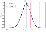
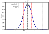
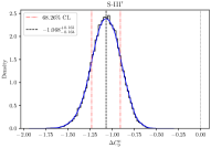
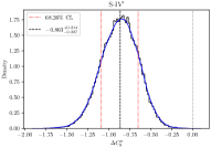
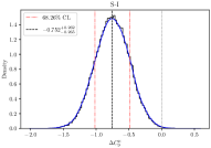
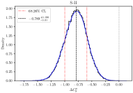
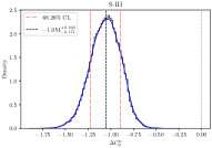
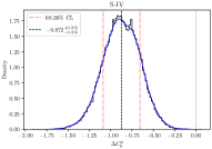
Figure 1: Density(black steps) and Kernel Density Estimation KDE (blue curves) of Wilson coefficients $\Delta C_{9}^{\mu}$ in different scenarios varied from old Dataset A to B. Red(dotdashed) lines indicate the Highest Posterior Density (HPD) about 68.26% which give the error estimations. Black(dashed) lines refer to the Bayesian estimations of $\Delta C_{9}^{\mu}$ while gray(dotted) lines refer to SM positions.

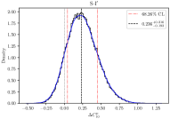
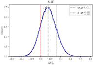
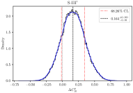
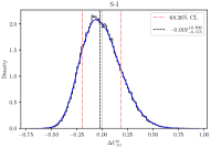
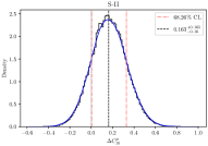
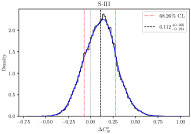
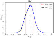
Figure 2: Density(black steps) and KDE (blue curves) of Wilson coefficients $\Delta C_{10}^{\mu}$ in different scenarios varied from old Dataset A to B. Intervals between the two red(dotdashed) lines cover the HPD about 68.26% to estimate 1$\sigma$ range. The remained indicators black(dashed) and gray(dotted) lines play the similar role as the description of Fig. 1.

Table 3: Global fits in various scenarios based on Dataset A with $\chi^{2}_{\text{SM}}=287.424$ which calculated by setting all WCs to be zero as well as corresponding observables n=201.

Params S-I’ S-II’ S-III’ S-IV’ ACDMN[23] AS[24] HMMN[25] GGJLCS [26] Reduced $\chi^{2}$ 183.404/(n-12) 197.556/(n-12) 182.869/(n-16) 176.807/(n-20) 260.66/(254-6) 179.1/(183-20) 96.88/90 $\chi^{2}_{\text{min}}/\text{d.o.f}$ = 0.970 = 1.045 = 0.988 = 0.977 = 1.05 = 1.1 = 1.08 $\Delta C_{7}$ $-0.003^{+0.020}_{-0.019}$ $-0.001^{+0.015}_{-0.015}$ - $0.001^{+0.016}_{-0.015}$ $0.00_{-0.02}^{+0.01}$ - $0.06_{+0.03}^{-0.03}$ - $\Delta C_{7}^{\prime}$ $0.017^{+0.018}_{-0.019}$ $0.020^{+0.014}_{-0.015}$ - $0.020^{+0.014}_{-0.014}$ $+0.00_{-0.01}^{+0.02}$ - $-0.01_{+0.01}^{-0.01}$ - $\Delta C_{8}$ $-0.788^{+0.595}_{-0.514}$ $-0.885^{+0.435}_{-0.398}$ - $-0.773^{+0.451}_{-0.449}$ - - $-0.80_{+0.40}^{-0.40}$ - $\Delta C_{8}^{\prime}$ $-0.073^{+1.089}_{-1.000}$ $-0.093^{+0.921}_{-0.831}$ - $-0.089^{+0.996}_{-0.922}$ - - $-0.30_{-1.30}^{+1.30}$ - $\Delta C_{9}^{\mu}$ $-0.806^{+0.257}_{-0.272}$ $-0.795^{+0.205}_{-0.210}$ $-1.068^{+0.161}_{-0.164}$ $-0.863^{+0.214}_{-0.227}$ $-1.08_{-0.17}^{+0.18}$ $-0.82_{-0.23}^{+0.23}$ $-1.14_{+0.19}^{-0.19}$ $-1.07_{-0.29}^{+0.29}$ $\Delta C_{9}^{\prime\mu}$ $0.194^{+0.395}_{-0.416}$ $0.056^{+0.338}_{-0.342}$ $0.112^{+0.393}_{-0.397}$ $0.020^{+0.346}_{-0.362}$ $0.16_{-0.36}^{+0.37}$ $-0.10_{-0.34}^{+0.34}$ $0.05_{-0.32}^{+0.32}$ $0.32_{+0.21}^{-0.21}$ $\Delta C_{10}^{\mu}$ $0.236^{+0.216}_{-0.193}$ $0.145^{+0.166}_{-0.156}$ $0.164^{+0.181}_{-0.180}$ $0.213^{+0.166}_{-0.155}$ $0.15_{-0.13}^{+0.13}$ $+0.14_{-0.23}^{+0.23}$ $0.21_{+0.20}^{-0.20}$ $0.21_{+0.14}^{-0.14}$ $\Delta C_{10}^{\prime\mu}$ $-0.096^{+0.251}_{-0.237}$ $-0.108^{+0.186}_{-0.177}$ $-0.115^{+0.200}_{-0.198}$ $-0.089^{+0.177}_{-0.176}$ $-0.18_{-0.18}^{+0.20}$ $-0.33_{-0.23}^{+0.23}$ $-0.03_{-0.19}^{+0.19}$ $-0.26_{+0.14}^{-0.14}$ $\Delta C_{S}^{\mu}$ $0.066^{+1.091}_{-1.142}$ $-0.004^{+1.102}_{-1.131}$ $-0.008^{+0.883}_{-0.899}$ $-0.043^{+0.842}_{-0.875}$ - - $0.01_{-0.05}^{+0.05}$ - $\Delta C_{S}^{\prime\mu}$ $0.065^{+1.087}_{-1.140}$ $0.003^{+1.103}_{-1.126}$ $-0.002^{+0.873}_{-0.936}$ $-0.059^{+0.844}_{-0.869}$ - - $-0.01_{-0.05}^{+0.05}$ - $\Delta C_{P}^{\mu}$ $0.167^{+1.172}_{-1.225}$ $1.017^{+0.735}_{-0.816}$ $0.092^{+1.076}_{-0.994}$ $0.117^{+0.847}_{-0.894}$ - - $-0.04_{-0.02}^{+0.02}$ - $\Delta C_{P}^{\prime\mu}$ $0.053^{+1.169}_{-1.227}$ $0.891^{+0.729}_{-0.812}$ $0.010^{+1.083}_{-1.002}$ $0.040^{+0.854}_{-0.895}$ - - $-0.04_{-0.02}^{+0.02}$ - $\Delta C_{9}^{e}$ - $-0.795^{+0.205}_{-0.210}$ $-1.753^{+0.781}_{-0.772}$ $-1.551^{+0.627}_{-0.599}$ - $-0.24_{-1.17}^{+1.17}$ $-6.50_{-1.90}^{+1.90}$ - $\Delta C_{9}^{\prime e}$ - $0.056^{+0.338}_{-0.342}$ $1.725^{+1.724}_{-2.286}$ $1.710^{+1.466}_{-1.764}$ - - $1.40_{-2.30}^{+2.30}$ - $\Delta C_{10}^{e}$ - $0.145^{+0.166}_{-0.156}$ $0.108^{+1.456}_{-0.661}$ $0.058^{+1.193}_{-0.661}$ - $-0.24_{-0.78}^{+0.78}$ $\sim 0$ - $\Delta C_{10}^{\prime e}$ - $-0.108^{+0.186}_{-0.177}$ $0.600^{+1.208}_{-1.099}$ $0.655^{+0.958}_{-0.841}$ - - $\sim 0$ - $\Delta C_{S}^{e}$ - $-0.004^{+1.102}_{-1.131}$ $-0.719^{+1.861}_{-1.227}$ $-0.549^{+1.602}_{-1.232}$ - - $-0.38_{-0.41}^{+0.41}$ - $\Delta C_{S}^{\prime e}$ - $0.003^{+1.103}_{-1.126}$ $-0.699^{+1.837}_{-1.224}$ $-0.550^{+1.618}_{-1.326}$ - - $-0.36_{-0.50}^{+0.50}$ - $\Delta C_{P}^{e}$ - $1.017^{+0.735}_{-0.816}$ $-1.592^{+1.552}_{-1.079}$ $-1.688^{+1.366}_{-0.978}$ - - $-0.98_{-0.21}^{+0.21}$ - $\Delta C_{P}^{\prime e}$ - $0.891^{+0.729}_{-0.812}$ $-1.360^{+1.318}_{-1.149}$ $-1.431^{+1.212}_{-1.017}$ - - $-0.95_{-0.29}^{+0.29}$ -

To interpret the 2022 release of $R_{K^{(*)}}$ in a global picture of $b\to s\ell^{+}\ell^{-}$, we carry out global fits in four aforementioned scenarios based on two different datasets, Dataset A and B. We use Figures 1 and 2 to illustrate the central values and errors of typical parameters, $\Delta C_{9}^{\mu}$ and $\Delta C_{10}^{\mu}$, with Bayesian statistics. The first row of figures in Figures 1 and 2 are produced based on the early Dataset A, while the second row corresponds to Dataset B. The central values of the parameters, mainly located at around well-known $-1$ and $0.2$, differ slightly from scenarios in both two sets of fits. On the other hand, to understand how the global change occurs due to the 2022 update of $R_{K^{(*)}}$, a comparison between the results of the two datasets is necessary. Taking $\Delta C_{9}^{\mu}$ shown in Figure 1 as an example, the central values in all the scenarios vary, but not dramatically, while the errors almost keep unchanged.

Table 4: Global fits in various scenarios based on Dataset B with $\chi^{2}_{\text{SM}}=265.888$ originated from $\Delta C_{i}=0$ and the number of observables n=203.

Params S-I S-II S-III S-IV ADCMN[23] AS[24] HMMN[25] GGJLCS[26] Reduced $\chi^{2}$ 190.044/(n-12) 177.891/(n-12) 185.386/(n-16) 178.953/(n-20) 260.66/(254-6) 179.1/(183-20) 96.88/90 $\chi^{2}_{\text{min}}/\text{d.o.f}$ = 0.995 = 0.931 = 0.991 = 0.978 = 1.05 = 1.1 = 1.08 $\Delta C_{7}$ $-0.000^{+0.020}_{-0.020}$ $-0.001^{+0.015}_{-0.015}$ - $-0.000^{+0.016}_{-0.015}$ $0.00_{-0.02}^{+0.01}$ - $0.06_{+0.03}^{-0.03}$ - $\Delta C_{7}^{\prime}$ $0.017^{+0.020}_{-0.018}$ $0.020^{+0.015}_{-0.014}$ - $0.023^{+0.014}_{-0.016}$ $+0.00_{-0.01}^{+0.02}$ - $-0.01_{+0.01}^{-0.01}$ - $\Delta C_{8}$ $-0.995^{+0.540}_{-0.463}$ $-0.921^{+0.443}_{-0.378}$ - $-0.773^{+0.465}_{-0.424}$ - - $-0.80_{+0.40}^{-0.40}$ - $\Delta C_{8}^{\prime}$ $-0.080^{+1.046}_{-0.942}$ $-0.076^{+0.893}_{-0.833}$ - $-0.258^{+1.007}_{-0.802}$ - - $-0.30_{-1.30}^{+1.30}$ - $\Delta C_{9}^{\mu}$ $-0.752^{+0.262}_{-0.265}$ $-0.789^{+0.198}_{-0.210}$ $-1.054^{+0.163}_{-0.171}$ $-0.872^{+0.215}_{-0.215}$ $-1.08_{-0.17}^{+0.18}$ $-0.82_{-0.23}^{+0.23}$ $-1.14_{+0.19}^{-0.19}$ $-1.07_{-0.29}^{+0.29}$ $\Delta C_{9}^{\prime\mu}$ $0.174^{+0.434}_{-0.441}$ $0.048^{+0.338}_{-0.348}$ $0.130^{+0.439}_{-0.437}$ $0.088^{+0.342}_{-0.378}$ $0.16_{-0.36}^{+0.37}$ $-0.10_{-0.34}^{+0.34}$ $0.05_{-0.32}^{+0.32}$ $0.32_{+0.21}^{-0.21}$ $\Delta C_{10}^{\mu}$ $-0.019^{+0.206}_{-0.175}$ $0.163^{+0.165}_{-0.160}$ $0.112^{+0.166}_{-0.184}$ $0.171^{+0.157}_{-0.175}$ $0.15_{-0.13}^{+0.13}$ $+0.14_{-0.23}^{+0.23}$ $0.21_{+0.20}^{-0.20}$ $0.21_{+0.14}^{-0.14}$ $\Delta C_{10}^{\prime\mu}$ $-0.118^{+0.266}_{-0.247}$ $-0.093^{+0.183}_{-0.179}$ $-0.115^{+0.215}_{-0.213}$ $-0.062^{+0.197}_{-0.180}$ $-0.18_{-0.18}^{+0.20}$ $-0.33_{-0.23}^{+0.23}$ $-0.03_{-0.19}^{+0.19}$ $-0.26_{+0.14}^{-0.14}$ $\Delta C_{S}^{\mu}$ $0.023^{+1.064}_{-1.097}$ $0.060^{+1.188}_{-1.230}$ $-0.066^{+0.944}_{-0.929}$ $0.009^{+0.858}_{-0.845}$ - - $0.01_{-0.05}^{+0.05}$ - $\Delta C_{S}^{\prime\mu}$ $0.014^{+1.064}_{-1.086}$ $0.061^{+1.188}_{-1.225}$ $-0.070^{+0.957}_{-0.930}$ $0.012^{+0.858}_{-0.862}$ - - $-0.01_{-0.05}^{+0.05}$ - $\Delta C_{P}^{\mu}$ $0.079^{+1.159}_{-1.146}$ $0.478^{+0.808}_{-0.899}$ $0.189^{+1.018}_{-1.028}$ $0.124^{+0.902}_{-0.910}$ - - $-0.04_{-0.02}^{+0.02}$ - $\Delta C_{P}^{\prime\mu}$ $-0.032^{+1.158}_{-1.145}$ $0.370^{+0.803}_{-0.897}$ $0.098^{+1.009}_{-1.024}$ $0.038^{+0.894}_{-0.913}$ - - $-0.04_{-0.02}^{+0.02}$ - $\Delta C_{9}^{e}$ - $-0.789^{+0.198}_{-0.210}$ $-1.623^{+0.662}_{-0.734}$ $-1.511^{+0.561}_{-0.533}$ - $-0.24_{-1.17}^{+1.17}$ $-6.50_{-1.90}^{+1.90}$ - $\Delta C_{9}^{\prime e}$ - $0.048^{+0.338}_{-0.348}$ $1.090^{+1.610}_{-1.793}$ $0.864^{+1.483}_{-1.608}$ - - $1.40_{-2.30}^{+2.30}$ - $\Delta C_{10}^{e}$ - $0.163^{+0.165}_{-0.160}$ $0.555^{+1.042}_{-0.576}$ $0.383^{+0.840}_{-0.424}$ - $-0.24_{-0.78}^{+0.78}$ $\sim 0$ - $\Delta C_{10}^{\prime e}$ - $-0.093^{+0.183}_{-0.179}$ $0.088^{+0.969}_{-0.956}$ $0.002^{+0.881}_{-0.815}$ - - $\sim 0$ - $\Delta C_{S}^{e}$ - $0.060^{+1.188}_{-1.230}$ $-0.952^{+2.122}_{-1.139}$ $-0.806^{+1.900}_{-1.238}$ - - $-0.38_{-0.41}^{+0.41}$ - $\Delta C_{S}^{\prime e}$ - $0.061^{+1.188}_{-1.225}$ $-1.051^{+2.251}_{-1.075}$ $-0.803^{+1.861}_{-1.194}$ - - $-0.36_{-0.50}^{+0.50}$ - $\Delta C_{P}^{e}$ - $0.478^{+0.808}_{-0.899}$ $-1.568^{+1.544}_{-1.149}$ $-1.837^{+1.376}_{-0.930}$ - - $-0.98_{-0.21}^{+0.21}$ - $\Delta C_{P}^{\prime e}$ - $0.370^{+0.803}_{-0.897}$ $-1.477^{+1.409}_{-1.083}$ $-1.652^{+1.200}_{-0.979}$ - - $-0.95_{-0.29}^{+0.29}$ -

Incorporating all the WCs analyzed in various scenarios based on both Dataset A and B. We summarize the results of all the fitted parameters characterizing new physics effects in Tables 3 and 4, respectively. The numbers of fitted parameters in our analysis are two sets of 12, one set of 16, and 20, denoted as scenario I, II, III, and IV (S-I, S-II, S-III, and S-IV, or those corresponding ones with a prime). As a comparison, early global fits made by other four independent analyses [23, 24, 25, 26] (one group of 20-D, one group of 6-D, and two groups of 4-D parameters) are also listed in the two tables.

To confirm the correctness of our numerical calculation, we first perform a calculation based on Dataset A, as shown in Table 3, in different working scenarios (with a prime). Our fitted WCs of muon flavor are consistent not only with each scenario but also with the other four independent groups within the fitted errors. WCs involving electron flavor have been studied less, and early efforts can be found in the two groups AS[24] and HMMN[25]. With similar errors ($1.2$ and $1.9$) but obvious different central values ($-0.24$ and $-6.50$) for $\Delta C_{9}^{e}$, it is not easy to judge how its deviation from the SM prediction. Our calculations in both S-III’ ($-1.8\pm 0.8$) and S-IV’ ($-1.6\pm 0.6$) provide self-consistent information and support a negative deviation from the SM about $2.5\sigma$. As for $\Delta C_{10}^{e}$, it can be concluded that the deviation from the SM is within $1\sigma$, combining all our calculations (S-II’, III’, and IV’) as well as the work done by AS[24] and HMMN[25]. In general, the errors of scalar operator WCs in HMMN[25] are smaller than ours. Though we both make a consistent description (less than $2\sigma$ deviation) for $\Delta C_{S,P}^{(^{\prime})\mu}$ and $\Delta C_{S}^{(^{\prime})e}$, the feature of $\Delta C_{P}^{(^{\prime})e}$ differs. Our calculation prefers a SM-like behavior while HMMN[25] suggests a deviation of around $4\sigma$, requiring further clarification by incorporating more and more precise data as well as more efforts on fitting.

The impact of the 2022 $R_{K^{(*)}}$ data is detailed in Table 4. The new physics potential in $\Delta C_{9}^{\mu}$, which was highly anticipated before, has been widely questioned since the release of $R_{K^{(*)}}^{\text{2022}}$. According to the numerical results in Table 4, the roughly $4\sigma$ standard deviations still exist in each scenario, with slight shifts in central values and almost unchanged errors. The SM-like behavior of $\Delta C_{7,8}^{(^{\prime})}$, within a $2\sigma$ deviation, remains unchanged from the earlier data. The situation for other muon flavor related fitted parameters depends on the number of fitting parameters. For example, the fitted $\Delta C_{9}^{\mu}$ in S-III exhibits a decreased standard deviation from $6.6\sigma$ in Dataset A to $6.4\sigma$ in Dataset B. Therefore, it can be safely said that all the muon type WCs except $\Delta C_{9}^{\mu}$ are all within $2\sigma$ deviations. Moreover, the updated $\Delta C_{9}^{e}$ values are consistent with the previous values shown in Table 3. The deviation in Scenario III still keeps around $2.3\sigma$, with both slight decreased central value and error.

$\begin{array}[]{cc}(a)&(b)\\ \includegraphics[width=182.1196pt]{muC9_eC9.pdf}&\includegraphics[width=182.1196pt]{muC10_eC10.pdf}\\ (c)&(d)\\ \includegraphics[width=182.1196pt]{muCS_eCS.pdf}&\includegraphics[width=182.1196pt]{muCP_eCP.pdf}\par\end{array}$

Figure 3: The correlations of corresponding WCs specified by their lepton flavors with a consideration of $R_{K^{(*)}}^{\text{2022}}$, taking an example of left-handed operators. The red(dotted) and green(dotdashed) regions represent the S-IV as well as S-III, where darker/lighter part are their corresponding 1/2$\sigma$ regions. Markers circle(square) are estimations of WCs in S-IV(S-III), respectively. The absence of S-II and S-I due to their WCs are not fully independent we set to be.

The deviation in Scenario IV shifts from $2.6\sigma$ to $2.8\sigma$. All other electron type WCs, including $\Delta C_{10,S,P}^{(^{\prime})e}$, are found to be restricted within around $1\sigma$.

In addition to the 1-D parameter projections from the high dimensional full parameter space shown in Tables 3 and 4, more information can be drawn from correlations among 2-D parameters. In many previous studies, lepton flavors in $\mathcal{O}_{9,10}^{(^{\prime})}$ as well as $\mathcal{O}_{S,P}^{(^{\prime})}$ are usually not discriminated. This assumption is also adopted as one of our working scenarios (S-II or S-II’). However, it is important to keep in mind that relaxing the identical lepton flavor restriction is also possible. We present explicitly in Fig. 3, the correlations between WCs of the same type among by specifying the lepton flavors in Scenario III and IV based on Dataset B. The locations of the best fit points and the $1\sigma$ allowed regions are dependent on the working scenario, as shown by the analysis of left-handed operators in Figure 3. A straight line passing through the origin with a slope of 1 represents lepton flavor independence. In

$\begin{array}[]{cc}(a)&(b)\\ \includegraphics[width=182.1196pt]{muC9_muC9_prime.pdf}&\includegraphics[width=182.1196pt]{muC10_muC10_prime.pdf}\\ (c)&(d)\\ \includegraphics[width=182.1196pt]{muCS_muCS_prime.pdf}&\includegraphics[width=182.1196pt]{muCP_muCP_prime.pdf}\\ (e)&(f)\\ \includegraphics[width=182.1196pt]{eCS_eCS_prime.pdf}&\includegraphics[width=182.1196pt]{eCP_eCP_prime.pdf}\end{array}$

Figure 4: The correlations of corresponding WCs distinct from their chirality incorporating the updated $R_{K^{(*)}}$, with a consideration of muon type operators ((a)-(d)) and typical electron type operators ((e)-(f)). The orange(solid), purple(dashed), green(dotdashed) and red(dotted) regions represent S-I, S-II, S-III and S-IV, respectively. The description of absence of S-I and S-II follows the Fig. 3.

almost all of the two scenarios (S-III and S-IV), $\Delta C_{9}$ and $\Delta C_{S,P}$ deviate from this line in the $1\sigma$ region, while $\Delta C_{10}$ contains part of the ”flavor identical line” in its $1\sigma$ region. But in $2\sigma$ regions, the flavor identical line can be contained by all $\Delta C_{9,10}$ and $\Delta C_{S,P}$. Therefore, at the $1\sigma$ level, the identical lepton flavor is only respected by $\Delta C_{10}$ but can be extended to all at the $2\sigma$ level.

$\begin{array}[]{cc}(a)&(b)\\ \includegraphics[width=182.1196pt]{muC9_muC10.pdf}&\includegraphics[width=182.1196pt]{eC9_eC10.pdf}\end{array}$

Figure 5: The correlations of WCs involving more than $3\sigma$ deviations from SM predictions with the $R_{K^{(*)}}^{\text{2022}}$. Conventions of color, linetypes and markers remain the same as those in Fig. 3 and 4.

The relations between operators with opposite chirality are also of interest. We show them in the form of 2-D correlations in Figure 4. Similar to the flavor situation, we take the line with slope of 1 and intercept of 0 as a criterion to judge the chirality dependence from data. Apparently, the deviations of such a line, at the $2\sigma$ level, in all the four scenarios of $\Delta C_{9}^{\mu}$ indicate that $\Delta C_{9}^{\mu}$ and $\Delta C_{9}^{{}^{\prime}\mu}$ are indeed two separated parameters. As for $\Delta C_{10}^{\mu}$, the identical chirality is not excluded at the $1\sigma$ region in S-I, and can be kept at the $2\sigma$ regions in all the 4 scenarios. A strict respect of the criterion line can be found for the WCs of two scalar operators ($\Delta C_{S}$ and $\Delta C_{P}$) shown as (c) and (d) in Figure 4. This indicates that the chirality is indistinguishable for the two muon type scalar operators, although their fitted sizes are SM-like. Due to the limited data about channels involving electrons, the surviving areas for $\Delta C_{S}^{e}-\Delta C_{S}^{{}^{\prime}e}$ and $\Delta C_{P}^{e}-\Delta C_{P}^{{}^{\prime}e}$ are much wider than the muon type operators, with the identical chirality line contained. Their sizes, which are consistent with SM at $2\sigma$ level, and the chirality relations are anticipated to be improved more precisely when more data is accumulated.

III.3 Discussions

Throughout the analyses in this work, the most important issue is whether the new physics possibility still exists by incorporating $R_{K^{(*)}}^{\text{2022}}$. As shown in Fig. 5 explicitly, although $\Delta C_{10}$ agrees with SM within $1\sigma$ in all the four scenarios for both muon and electron type, deviations from SM in $\Delta C_{9}^{\mu}$ indeed exist for more than $4\sigma$ for most scenarios and $\Delta C_{9}^{e}$ for around $3\sigma$ in Scenario II.

The scalar operators are in general with small central values but large uncertainties as shown in Table 3 and 4. The 2-D correlations shown in Fig. 4 apparently indicate the strong linear relations

$$\Delta C_{S}^{\mu}=\Delta C_{S}^{{}^{\prime}\mu},\quad\Delta C_{P}^{\mu}=\Delta C_{P}^{{}^{\prime}\mu}.$$ (18)

On the other hand, if the emergence of new physics is described within the framework of SMEFT, the relations

$$\Delta C_{S}^{\mu}=-\Delta C^{\mu}_{P},\quad\Delta C^{{}^{\prime}\mu}_{S}=\Delta C^{{}^{\prime}\mu}_{P}$$ (19)

hold up to dimension-6 operators [70], leading to

$$\Delta C_{S}^{(^{\prime})\mu}=\Delta C_{P}^{(^{\prime})\mu}=0.$$ (20)

Note this feature for null scalar operators may violate in other non-SMEFT new physics[71].

IV Concluding Remarks

In this work, we perform global fits to two sets of datasets, one before and one after the release of $R_{K^{(*)}}^{\text{2022}}$ (denoted as Dataset A and B), in four sets of working scenarios. In some of the working scenarios, we distinguish lepton flavor, which results in as many as 20 fitted parameters. Our numerical analysis based on Bayesian statistics helps to interpret data and the following points can be concluded incorporating $R_{K^{(*)}}^{\text{2022}}$. (i) The new physics possibility still exists. As explicitly shown in Fig. 5, current data still supports a deviation about or more than $4\sigma$ from SM for $\Delta C_{9}^{\mu}$. (ii) The interpretation of flavor dependence in WCs is improved. At $1\sigma$ level, the muon and electron flavor is distinguishable for $\Delta C_{9,S,P}$ but indistinguishable for $\Delta C_{10}$. And if allowing $2\sigma$ errors, lepton flavor is indistinguishable for all the four operators and their corresponding WCs $\Delta C_{9,10,S,P}$. (iii) The relation between operators and their chiral dual ones is specified. The WCs for scalar operators $\Delta C_{S}^{\mu}$ and $\Delta C_{P}^{\mu}$ are strictly chirality independent. At $1\sigma$ level, the data also indicates that to distinguish chirality is not necessary for $\Delta C_{S}^{e}$ and $\Delta C_{P}^{e}$. The WC $\Delta C_{9}^{\mu}$ differs from its dual one $\Delta C_{9}^{{}^{\prime}\mu}$ at $2\sigma$ level in all the four scenarios, while $\Delta C_{10}^{\mu}$ distinguishes $\Delta C_{10}^{{}^{\prime}\mu}$ in three of the four scenarios. (iv) If the emergence of new physics is in terms of SMEFT, the scalar operators vanish.

Although the working scenario dependence indeed exists by comparing with detailed scenarios, it does not change the main features of global fits. The obtained results from current model independent fits provide useful inputs for new physics models or help to discriminate some of the models.

Appendix A Formulas for Involved Observables

In this part, we provided a list about calculation of all observables we used in analysis, more detailed discussions are found in corresponding subsection.

A.1 $B_{s,d}\to\ell\ell$

It is worth pointing out that our formula deduced previously called CP-averaged or ’experimental’ branching ratio. The untagged or ”theoretical” branching ratio is different from previous one through[72]

$$\text{BR}^{\text{untag}}(B_{s}\to\mu^{+}\mu^{-})=\left[\frac{1+\mathcal{A}_{\Delta\Gamma}y_{s}}{1-y_{s}^{2}}\right]\text{BR}(B_{s}\to\mu^{+}\mu^{-}),$$ (21)

$$\mathcal{A}_{\Delta\Gamma}=\frac{|k_{P}|^{2}\cos(2\varphi_{P})-|k_{S}|^{2}\cos(2\varphi_{S})}{|k_{P}|^{2}+|k_{S}|^{2}},$$

with $k_{S},k_{P},\varphi_{S},\varphi_{P}$ which are given in[72].

A.2 $B\to V\ell^{+}\ell^{-}$ formulae

The full angular decay distribution of $\bar{B}^{0}\to\bar{K}^{*0}\ell^{+}\ell^{-}$ which obtained from Buras[30] is shown as

$$\frac{{\text{d}}^{4}\Gamma^{\ell}}{{\text{d}}q^{2}~{}{\text{d}}\cos\theta_{\ell}~{}{\text{d}}\cos\theta_{K^{*}}~{}{\text{d}}\phi}=\frac{9}{32\pi}J^{\ell}\left(q^{2},\theta_{\ell},\theta_{K^{*}},\phi\right),$$ (22)

where

$$J^{\ell}\left(q^{2},\theta_{\ell},\theta_{K^{*}},\phi\right) =J_{1;s}^{\ell}\sin^{2}\theta_{K^{*}}+J_{1;c}^{\ell}\cos^{\theta}_{K^{*}}+\left(J_{2;s}^{\ell}\sin^{2}\theta_{K^{*}}+J_{2;c}^{\ell}\cos^{2}\theta_{K^{*}}\right)\cos 2\theta_{\ell}$$ (23)

$$+J_{3}^{\ell}\sin^{2}\theta_{K^{*}}\sin^{2}\theta_{\ell}\cos 2\phi+J_{4}^{\ell}\sin 2\theta_{K^{*}}\sin 2\theta_{\ell}\cos\phi$$

$$+J_{5}^{\ell}\sin 2\theta_{K^{*}}\sin\theta_{\ell}\cos\phi$$

$$+\left(J_{6;s}^{\ell}\sin^{2}\theta_{K^{*}}+J_{6;c}^{\ell}\cos^{2}\theta_{K^{*}}\right)\cos\theta_{\ell}+J_{7}^{\ell}\sin 2\theta_{K^{*}}\sin\theta_{\ell}\sin\phi$$

$$+J_{8}^{\ell}\sin 2\theta_{K^{*}}\sin 2\theta_{\ell}\sin\phi+J_{9}^{\ell}\sin^{2}\theta_{K^{*}}\sin^{2}\theta_{\ell}\sin 2\phi$$

The corresponding expression for the CP-conjugated mode $B^{0}\to K^{*0}\ell^{+}\ell^{-}$ is obtained form Eq.(23) by the replacements $J^{(a)}_{1,2,3,4,7;\ell}\to\bar{J}^{(a)}_{1,2,3,4,7;\ell},~{}J^{(a)}_{5,6,8,9;\ell}\to-\bar{J}^{(a)}_{5,6,8,9;\ell}.$ With the eight transverse amplitudes defined in the consecutive subsection, the angular coefficients $J_{i}$ in (9) can be written as

$$J_{1;s}^{\ell} =\frac{(2+\beta_{\ell}^{2})}{4}\left[|A_{\perp;\ell}^{\text{L}}|^{2}+|A_{\parallel;\ell}^{\text{L}}|^{2}+\left(\text{L}\to\text{R}\right)\right]+\frac{4m_{\ell}^{2}}{q^{2}}\Re\left(A_{\perp;\ell}^{\text{L}}A_{\perp;\ell}^{\text{R${}^{\ast}$}}+A_{\parallel;\ell}^{\text{L}}A_{\parallel;\ell}^{\text{R${}^{\ast}$}}\right),$$ (24)

$$J_{1;c}^{\ell} =|A_{0;\ell}^{\text{L}}|^{2}+|A_{0;\ell}^{\text{R}}|^{2}+\frac{4m_{\ell}^{2}}{q^{2}}\left[|A_{t;\ell}|^{2}+2\Re\left(A_{0;\ell}^{\text{L}}A_{0;\ell}^{\text{R${}^{\ast}$}}\right)\right]+\beta^{2}_{\ell}|A_{\text{S};\ell}|^{2},$$

$$J_{2;s}^{\ell} =\frac{\beta_{\ell}^{2}}{4}\left[|A_{\perp;\ell}^{\text{L}}|^{2}+|A_{\parallel;\ell}^{\text{L}}|^{2}+\left(\text{L}\to\text{R}\right)\right],\quad J_{2;c}^{\ell}=-\beta_{\ell}^{2}\left[|A_{0;\ell}^{\text{L}}|^{2}+\left(\text{L}\to\text{R}\right)\right],$$

$$J_{3}^{\ell} =\frac{1}{2}\beta_{\ell}^{2}\left[|A_{\perp;\ell}^{\text{L}}|^{2}-|A_{\parallel;\ell}^{\text{L}}|^{2}+\left(\text{L}\to\text{R}\right)\right],\quad J_{4}^{\ell}=\frac{1}{\sqrt{2}}\beta_{\ell}^{2}\left[\Re\left(A_{0;\ell}^{\text{L}}A_{\parallel;\ell}^{\text{L${}^{\ast}$}}\right)+\left(\text{L}\to\text{R}\right)\right],$$

$$J_{5}^{\ell} =\sqrt{2}\beta_{\ell}\left[\Re\left(A_{0;\ell}^{\text{L}}A_{\perp;\ell}^{\text{L${}^{\ast}$}}\right)-\left(\text{L}\to\text{R}\right)-\frac{m_{\ell}}{\sqrt{q^{2}}}\Re\left(A_{\parallel;\ell}^{\text{L}}A_{\text{S};\ell}^{\ast}+A_{\parallel;\ell}^{\text{R}}A_{\text{S};\ell}^{\ast}\right)\right],$$

$$J_{6;s}^{\ell} =2\beta_{\ell}\left[\Re\left(A_{\parallel;\ell}^{\text{L}}A_{\perp;\ell}^{\text{L${}^{\ast}$}}\right)-\left(\text{L}\to\text{R}\right)\right],\quad J_{6;c}^{\ell}=4\beta_{\ell}\frac{m_{\ell}}{\sqrt{q^{2}}}\left[\Re\left(A_{0;\ell}^{\text{L}}A_{\text{S};\ell}^{\text{${}^{\ast}$}}\right)+\left(\text{L}\to\text{R}\right)\right],$$

$$J_{7}^{\ell} =\sqrt{2}\beta_{\ell}\left[\Im\left(A_{0;\ell}^{\text{L}}A_{\parallel;\ell}^{\text{L${}^{\ast}$}}\right)-\left(\text{L}\to\text{R}\right)+\frac{m_{\ell}}{\sqrt{q^{2}}}\Im\left(A_{\perp;\ell}^{\text{L}}A_{\text{S};\ell}^{\ast}+A_{\perp;\ell}^{\text{R}}A_{\text{S};\ell}^{\ast}\right)\right],$$

$$J_{8}^{\ell} =\frac{1}{\sqrt{2}}\beta_{\ell}^{2}\left[\Im\left(A_{0;\ell}^{\text{L}}A_{\perp;\ell}^{\text{L${}^{\ast}$}}\right)+\left(\text{L}\to\text{R}\right)\right],\quad J_{9}^{\ell}=\beta_{\ell}^{2}\left[\Im\left(A_{\parallel;\ell}^{\text{L${}^{\ast}$}}A_{\perp;\ell}^{\text{L}}\right)+\left(\text{L}\to\text{R}\right)\right],$$

which further rely on various helicity amplitudes, giving

$$A_{\perp;\ell}^{\text{L,R}} =N_{0}^{\ell}\sqrt{2}\lambda M_{B}^{2}\left[\left[\left(C_{9}^{\ell}+C_{9}^{\prime\ell}\right)\mp\left(C_{10}^{\ell}+C_{10}^{\prime\ell}\right)\right]\frac{V(q^{2})}{M_{B}+M_{K^{\ast}}}\right.$$ (25)

$$\hskip 113.81102pt\left.+\frac{2m_{b}}{q^{2}}\left(C_{7}^{\ell}+C_{7}^{\prime\ell}\right)T_{1}\left(q^{2}\right)\right]+\Delta A_{\perp}^{\text{L,R}},$$

$$A_{\parallel;\ell}^{\text{L,R}} =-N_{0}^{\ell}\sqrt{2}\left(M_{B}^{2}-M_{K^{\ast}}^{2}\right)\left[\left[\left(C_{9}^{\ell}-C_{9}^{\prime\ell}\right)\mp\left(C_{10}^{\ell}-C_{10}^{\prime\ell}\right)\right]\frac{A_{1}(q^{2})}{M_{B}-M_{K^{\ast}}}\right.$$

$$\hskip 113.81102pt\left.\quad+\frac{2m_{b}}{q^{2}}\left(C_{7}^{\ell}-C_{7}^{\prime\ell}\right)T_{2}\left(q^{2}\right)\right]+\Delta A_{\parallel}^{\text{L,R}},$$

$$A_{0;\ell}^{\text{L,R}} =\frac{-N_{0}^{\ell}}{2M_{K^{\ast}}\sqrt{q^{2}}}\left\{\left[\left(C_{9}^{\ell\prime}-C_{9}^{\prime\ell}\right)\mp\left(C_{10}^{\ell}-C_{10}^{\prime\ell}\right)\right]\right.$$

$$\quad\left.\times\left[(M_{B}^{2}-M_{K^{\ast}}^{2}-q^{2})(M_{B}+M_{K^{\ast}})A_{1}(q^{2})-\lambda^{2}M_{B}^{4}\frac{A_{2}\left(q^{2}\right)}{M_{B}+M_{K^{\ast}}}\right]\right.$$

$$\quad\left.+2m_{b}\left(C^{\ell}_{7}-C_{7}^{\prime\ell}\right)\left[(M_{B}^{2}+3M_{K^{\ast}}^{2}-q^{2})T_{2}\left(q^{2}\right)-\frac{\lambda^{2}M_{B}^{4}}{M_{B}^{2}-M_{K^{\ast}}^{2}}T_{3}\left(q^{2}\right)\right]\right\}+\Delta A_{0}^{\text{L,R}},$$

$$A_{t;\ell}=\frac{N_{0}^{\ell}}{\sqrt{q^{2}}}\lambda M_{B}^{2}\left[2\left(C_{10}^{\ell}-C_{10}^{\prime\ell}\right)+\frac{q^{2}}{m_{\ell}}\left(C^{\ell}_{P}-C^{\prime\ell}_{P}\right)\right]A_{0}\left(q^{2}\right),\hskip 113.81102pt$$ (26)

$$A_{\text{S};\ell}=-2N_{0}^{\ell}\lambda M_{B}^{2}\left(C^{\ell}_{\text{S}}-C^{\prime\ell}_{\text{S}}\right)A_{0}\left(q^{2}\right),$$

associated with the constant

$$N^{0}_{\ell}=V_{tb}V_{ts}^{\ast}\left[\frac{G_{F}^{2}\alpha^{2}}{3\cdot 2^{10}\pi^{5}M_{B}}q^{2}\lambda\beta_{\ell}\right]^{\frac{1}{2}}$$ (27)

and parameters $\lambda$ and $\beta_{\mu}$ defined as

$$\beta_{\ell} =\sqrt{1-4\frac{m_{\ell}^{2}}{q^{2}}},~{}~{}\lambda\left(q^{2},M_{K}^{2}\right)=\left[\left(1-\frac{q^{2}}{M_{B}^{2}}\right)^{2}-2\frac{m_{K}^{2}}{M_{B}^{2}}\left(1+\frac{q^{2}}{M_{B}^{2}}\right)+\frac{m_{K}^{4}}{M_{B}^{4}}\right]^{\frac{1}{2}}.$$

The corrections $\Delta A$ in Eq. (26), originating from weak annihilation and spectator scattering [41], are given as

$$\Delta A_{\perp}^{L;R} =\frac{2\sqrt{2}\lambda Nm_{b}M_{B}^{2}}{q^{2}}\left(\mathcal{T}_{\perp}^{(t),\text{nf+WA}}+\frac{\lambda_{u}}{\lambda_{t}}\mathcal{T}_{\perp}^{(u)}\right),$$ (28)

$$\Delta A_{\parallel}^{L;R} =\frac{-2\sqrt{2}E_{V}Nm_{b}(M_{B}^{2}-M_{V}^{2})}{q^{2}M_{B}}\left(\mathcal{T}_{\perp}^{(t),\text{nf+WA}}+\frac{\lambda_{u}}{\lambda_{t}}\mathcal{T}_{\perp}^{(u)}\right),$$

$$\Delta A_{0}^{L;R} =-\frac{NM_{B}^{2}m_{b}}{\sqrt{q^{2}}M_{V}}\left\{\left[\left(M_{B}^{2}+3M_{V}^{2}-q^{2}\right)\frac{2E_{V}}{M_{B}^{3}}-\frac{\lambda^{2}M_{B}^{2}}{M_{B}^{2}-M_{V}^{2}}\right]\times\left(\mathcal{T}_{\perp}^{(t),\text{nf+WA}}+\frac{\lambda_{u}}{\lambda_{t}}\mathcal{T}_{\perp}^{(u)}\right)\right.$$

$$\quad\left.-\frac{\lambda^{2}M_{B}^{2}}{M_{B}^{2}-M_{V}^{2}}\times\left(\mathcal{T}_{\parallel}^{(t),\text{nf+WA}}+\frac{\lambda_{u}}{\lambda_{t}}\mathcal{T}_{\parallel}^{(u)}\right)\right\},$$

with $\lambda_{i}\equiv V_{ib}V_{is}^{\ast}$ and $E_{V}=\frac{M_{B}^{2}+M_{V}^{2}-q^{2}}{2M_{B}}$. The amplitudes $\mathcal{T}_{\perp,\parallel}$ in Eq. (28), containing contributions from both non-factorizable hard-spectator scattering and weak annihilation, can be obtained by subtracting factorizable contributions from the invariant amplitude calculated in QCDF [21, 22, 73], giving

$$\mathcal{T}_{a}=\xi_{a}C_{a}+\frac{\pi^{2}}{N_{c}}\frac{f_{B}f_{V,a}}{MB}\Xi_{a}\sum_{\pm}\int_{0}^{\infty}\frac{d\omega}{\omega}\Phi_{B,\pm}(\omega)\int_{0}^{1}du\Phi_{K^{\ast},a}(u)T_{a,\pm}(u,\omega)$$ (29)

with $\Xi_{\parallel}=\frac{M_{V}}{E_{V}}$, $\Xi_{\perp}=1$, $N_{c}=3$ and

$$C_{a} =C_{a}^{(0)}+\frac{\alpha_{s}C_{F}}{4\pi}C_{a}^{(1)},$$ (30)

$$T_{a,\pm} =T_{a,\pm}^{(0)}+\frac{\alpha_{s}C_{F}}{4\pi}T_{a,\pm}^{(1)}.$$

In this work, we do not incorporate the long-distance effect generated from charm-loop, which has been considered in [74, 75]. In large energy limit (LEL), the number of heavy-to-light transition form factors can be reduced from $7$ to $2$, corresponding to transversal and longitudinal polarization of $K^{*}$. The correspondence between the two sets of form factors [76] is given as

$$V\left(q^{2}\right) =\left(1+\frac{M_{\text{vec}}}{M}\right)\xi_{\perp},\quad A_{1}\left(q^{2}\right)=\frac{2E}{M+M_{\text{vec}}}\xi_{\perp},$$ (31)

$$A_{2}\left(q^{2}\right) =\left(1+\frac{M_{\text{vec}}}{M}\right)\left[\xi_{\perp}-\frac{M_{\text{vec}}}{E}\xi_{\parallel}\right],\quad A_{0}\left(q^{2}\right)=\left(1-\frac{M_{\text{vec}}^{2}}{ME}\right)\xi_{\parallel}+\frac{M_{\text{vec}}}{M}\xi_{\perp},$$

$$T_{1}\left(q^{2}\right) =\xi_{\perp},\quad T_{2}\left(q^{2}\right)=\left(1-\frac{q^{2}}{M^{2}-M_{\text{vec}}^{2}}\right)\xi_{\perp},\quad T_{3}\left(q^{2}\right)=\xi_{\perp}-\frac{M_{\text{vec}}}{E}\left(1-\frac{M_{\text{vec}}^{2}}{M^{2}}\right)\xi_{\parallel},$$

where $M$ and $M_{\text{vec}}$ stand for B mesons as well as final state vector mesons, respectively. To solve $\xi_{\perp}$ and $\xi_{\parallel}$, we use form factors $T_{1}$ and $A_{0}$ [69] in the form of simplified series expansion (SSE) in our practical analysis.

A.3 $B\to P\ell^{+}\ell^{-}$

The angular distribution functions are described below[77]:

$$I_{a}^{\ell}\left(q^{2};C_{7,8,9,10,S,P}^{\prime}\right) =\frac{q^{2}}{M_{B}^{4}}\left(\beta_{\ell}^{3}|F^{\ell}_{S}|^{2}+\beta_{\ell}|F^{\ell}_{P}|^{2}\right)+\frac{\lambda}{4}\left(\lambda\beta_{\ell}|C^{\ell}_{10}|^{2}+\lambda\beta_{\ell}\Bigg{|}C^{\ell}_{9}+\frac{2m_{b}\mathcal{T}_{P}^{(0)}}{M_{B}\xi_{P}}\Bigg{|}^{2}\right)$$ (32)

$$\hskip 28.45274pt+\frac{2m_{\ell}\beta_{\ell}\left(M_{B}^{2}-M_{K}^{2}+q^{2}\right)\Re\left(F^{\ell}_{P}F^{\ell\ast}_{A}\right)}{M_{B}^{4}}+\frac{4m_{\ell}^{2}\beta_{\ell}|F^{\ell}_{A}|^{2}}{M_{B}^{2}},$$

$$I_{c}^{\ell}\left(q^{2};C_{7,8,9,10}^{\prime}\right) =-\frac{\lambda}{4}\left(\lambda\beta_{\ell}^{3}|C^{\ell}_{10}|^{2}+\lambda\beta_{\ell}^{3}\Bigg{|}C^{\ell}_{9}+\frac{2m_{b}\mathcal{T}_{P}}{M_{B}\xi_{P}}\Bigg{|}^{2}\right),$$

where form factors are defined as

$$F^{\ell}_{A}=C^{\ell}_{10},\qquad F^{\ell}_{T}=0,\qquad F^{\ell}_{T5}=0,$$ (33)

$$F^{\ell}_{P}=\frac{M_{B}^{2}-M_{K}^{2}}{2m_{b}(m_{b}-m_{s})}\frac{f_{0}}{f_{+}}(C_{P}^{\ell}+C_{P}^{\prime\ell})+m_{l}C^{\ell}_{10}\left[\frac{M_{B}^{2}-M_{K}^{2}}{q^{2}}\left(\frac{2E}{M_{B}}-1\right)-1\right],\qquad$$

$$F^{\ell}_{S}=\frac{M_{B}^{2}-M_{K}^{2}}{2m_{b}(m_{b}-m_{s})}\frac{f_{0}\left(q^{2}\right)}{f_{+}\left(q^{2}\right)}\left(C^{\ell}_{S}+C^{\prime\ell}_{S}\right),$$

$$F^{\ell}_{V}=C^{\ell}_{9}+\frac{2m_{b}}{M_{B}}\frac{\mathcal{T}_{P}\left(q^{2}\right)}{\xi_{P}\left(q^{2}\right)},\quad\frac{f_{0}}{f_{+}}=\frac{2E}{M_{B}}\left[1+\mathcal{O}(\alpha_{s})+\mathcal{O}\left(\frac{q^{2}}{M_{B}^{2}}\sqrt{\frac{\Lambda_{\text{QCD}}}{E}}\right)\right].$$

The invariant amplitude $\mathcal{T}_{P}$ has the form similar with $\mathcal{T}_{\parallel}$ in $B\to V\ell^{+}\ell^{-}$ [22]. We preserve the leading order and next-leading order non-factorizable contribution, giving

$$\mathcal{T}_{P}(q^{2})= \xi_{P}\left[\left(C_{7}^{eff}+C_{7}^{\prime eff}\right)+\frac{M_{B}}{2m_{b}}Y(q^{2})+\frac{\alpha_{s}C_{F}}{4\pi}C_{\parallel}^{nf}\right]$$ (34)

$$+\frac{\pi^{2}}{N_{c}}\frac{f_{B}f_{P}}{M_{B}}\sum_{\pm}\int_{0}^{\infty}\frac{d\omega}{\omega}\Phi_{B,\pm}(\omega)\int_{0}^{1}du\Phi_{K,\parallel}(u)\left[T_{\parallel,\pm}^{(0)}+\frac{\alpha_{s}C_{F}}{4\pi}\left(T_{\parallel,\pm}^{(nf)}\right)\right](u,\omega).$$

The form factors based on SSE [68, 74] can be parameterized as

$$\xi_{P} =f_{+}(q^{2})\equiv\frac{f_{+}(0)}{1-q^{2}/m^{2}_{\text{res}+}}\left\{1+a^{1}_{+}\left[z(q^{2})-z(0)+\frac{1}{2}\left(z(q^{2})^{2}-z(0)^{2}\right)\right]\right\},$$ (35)

$$z(q^{2}) =\frac{\sqrt{\tau_{+}-q^{2}}-\sqrt{\tau_{+}-\tau_{0}}}{\sqrt{\tau_{+}-q^{2}}+\sqrt{\tau_{+}-\tau_{0}}},~{}\tau_{0}=\sqrt{\tau_{+}}(\sqrt{\tau_{+}}-\sqrt{\tau_{+}-\tau_{-}}),~{}\tau_{\pm}=\left(M_{B}\pm M_{P}\right)^{2},$$

in which $f_{+}(q^{2}=0)$ can be calculated by LCSR and listed in Table 2.

A.4 $B\to X_{s}\ell^{+}\ell^{-}$

Here we give the definition of the important function $\tilde{N}$ in Eq. (11),

$$\tilde{N} \equiv~{}\left(1+\frac{2\hat{m}_{\ell}^{2}}{\hat{s}}\right)\left[|C_{9}^{\text{new}}|^{2}\left(1+2\hat{s}\right)\left(1+\frac{\alpha_{s}}{\pi}\tau_{99}(\hat{s})\right)+4|C_{7}^{\text{new}}|^{2}\left(1+\frac{2}{\hat{s}}\right)\left(1+\frac{\alpha_{s}}{\pi}\tau_{77}(\hat{s})\right)\right.$$ (36)

$$+\left.12\Re(C_{7}^{\text{new}}C_{9}^{\text{new}\ast})\left(1+\frac{\alpha_{s}}{\pi}\tau_{79}\left(\hat{s}\right)\right)\right]+|C_{10}^{\text{new}}|^{2}\left[\left(1+2\hat{s}\right)+\frac{2\hat{m}_{\ell}^{2}}{\hat{s}}\left(1-4\hat{s}\right)\right]\left(1+\frac{\alpha_{s}}{\pi}\tau_{99}\left(\hat{s}\right)\right)$$

$$+\frac{3}{2}|m_{b}C_{S}|^{2}\left(\hat{s}-4\hat{m}_{\ell}^{2}\right)+\frac{3}{2}|m_{b}C_{P}|^{2}\hat{s}+6\Re\left(m_{b}C_{10}^{\text{new}}C_{P}^{\ast}\right)\hat{m}_{\ell}+\left(C_{i}\leftrightarrow C_{i}^{\prime}\right),$$

where $\hat{m}_{\ell}$, $\hat{s}$ and $z$ has the form of

$$\hat{m}_{\ell}\equiv\frac{m_{\ell}}{m_{b;\text{pole}}},~{}\hat{s}\equiv\frac{s}{m_{b;\text{pole}}^{2}},~{}z\equiv\frac{m_{c;\text{pole}}^{2}}{m_{b;\text{pole}}^{2}}$$ (37)

and $\tau_{77}$, $\tau_{79}$ and $\tau_{99}$ have been calculated in [43]. Especially, $C_{7}^{\text{new}}$ and $C_{9}^{\text{new}}$ are defined as

$$C_{7}^{\text{new}}(s)=\left(1+\frac{\alpha_{s}}{\pi}\sigma_{7}(s)\right)C_{7}^{\text{eff}}-\frac{\alpha_{s}}{4\pi}\left[C_{1}F_{1}^{(7)}(s)+C_{2}F_{2}^{(7)}(s)+C_{8}^{\text{eff}}F_{8}^{(7)}(s)\right],$$ (38)

$$C_{9}^{\text{new}}(s)=\left(1+\frac{\alpha_{s}}{\pi}\sigma_{9}(s)\right)C_{9}^{\text{eff}}-\frac{\alpha_{s}}{4\pi}\left[C_{1}F_{1}^{(9)}(s)+C_{2}F_{2}^{(9)}(s)+C_{8}^{\text{eff}}F_{8}^{(9)}(s)\right],$$

$$C_{9}^{\text{new}}(s)=\left(1+\frac{\alpha_{s}}{\pi}\sigma_{9}(s)\right)C_{10}^{\text{eff}},$$

with $\sigma_{7},~{}\sigma_{9}$ given in [43] as well, and $F_{1;2;8}^{(7;9)}$ introduced in [22]. All the analytical formulas are well summarized in [41].

A.5 $\Lambda_{b}\to\Lambda\ell^{+}\ell^{-}$

With naive factorization approximation, the 10 angular distribution function in bottomed baryon decays can be expressed as,

$$J_{1ss} =\frac{1}{4}\left[|A_{\perp_{1}}^{R}|^{2}+|A_{\parallel_{1}}^{R}|^{2}+2|A_{\perp_{0}}^{R}|^{2}+2|A_{\parallel_{0}}^{R}|^{2}+(R\leftrightarrow L)\right],$$ (39)

$$J_{2ss} =\frac{\alpha_{\Lambda}}{2}\Re\left\{A_{\perp_{1}}^{R}A_{\parallel_{1}}^{\ast R}+2A_{\perp_{0}}^{R}A_{\parallel 0}^{\ast R}+(R\leftrightarrow L)\right\},$$

$$J_{1cc} =\frac{1}{2}\left[|A_{\perp_{1}}^{R}|^{2}+|A_{\parallel_{1}}^{R}|^{2}+\left(R\leftrightarrow L\right)\right],~{}~{}J_{1c}=-\Re\left\{A_{\perp_{1}}^{R}A_{\parallel_{1}}^{\ast R}-\left(R\leftrightarrow L\right)\right\},$$

$$J_{2cc} =+\alpha_{\Lambda}\Re\left\{A_{\perp_{1}}^{R}A_{\parallel_{1}}^{\ast R}+(R\leftrightarrow L)\right\},~{}~{}J_{2c}=-\frac{\alpha_{\Lambda}}{2}\left[|A_{\perp_{1}}^{R}|^{2}+|A_{\parallel_{1}}^{R}|^{2}-(R\leftrightarrow L)\right],$$

$$J_{3sc} =+\frac{\alpha_{\Lambda}}{\sqrt{2}}\Im\left\{A_{\perp_{1}}^{R}A_{\perp_{0}}^{\ast R}-A_{\parallel_{1}}^{R}A_{\parallel_{0}}^{\ast R}+(R\leftrightarrow L)\right\},~{}~{}J_{3s}=\frac{\alpha_{\Lambda}}{\sqrt{2}}\Re\left\{A_{\perp_{1}}^{R}A_{\parallel_{0}}^{\ast R}-A_{\parallel_{1}}^{R}A_{\perp_{0}}^{\ast R}+(R\leftrightarrow L)\right\},$$

$$J_{4sc} =+\frac{\alpha_{\Lambda}}{\sqrt{2}}\Im\left\{A_{\perp_{1}}^{R}A_{\perp_{0}}^{\ast R}-A_{\parallel_{1}}^{R}A_{\parallel_{0}}^{\ast R}-(R\leftrightarrow L)\right\},~{}~{}J_{4s}=\frac{\alpha_{\Lambda}}{\sqrt{2}}\Re\left\{A_{\perp_{1}}^{R}A_{\parallel_{0}}^{\ast R}-A_{\parallel_{1}}^{R}A_{\perp_{0}}^{\ast R}-(R\leftrightarrow L)\right\},$$

where $\alpha_{\Lambda}$ given in [58] and presented in Table 1. The definition of amplitudes $A$ can be further defined based on helicity amplitudes, giving

$$A_{\perp_{0}}^{L(R)} =+\sqrt{2}N_{1}\left(C_{9,10,+}^{L(R)}H_{0}^{V}\left(+1/2,+1/2\right)-\frac{2m_{b}(C_{7}+C_{7}^{\prime})}{q^{2}}H_{0}^{T}(+1/2,+1/2)\right),$$ (40)

$$A_{\parallel_{0}}^{L(R)} =-\sqrt{2}N_{1}\left(C_{9,10,+}^{L(R)}H_{0}^{A}\left(+1/2,+1/2\right)+\frac{2m_{b}(C_{7}-C_{7}^{\prime})}{q^{2}}H_{0}^{T5}(+1/2,+1/2)\right),$$

$$A_{\perp_{1}}^{L(R)} =+\sqrt{2}N_{1}\left(C_{9,10,+}^{L(R)}H_{+}^{V}(-1/2,+1/2)-\frac{2m_{b}(C_{7}+C_{7}^{\prime})}{q^{2}}H_{+}^{T}(-1/2,+1/2)\right),$$

$$A_{\parallel_{1}}^{L(R)} =-\sqrt{2}N_{1}\left(C_{9,10,-}^{L(R)}H_{+}^{A}\left(-1/2,+1/2\right)+\frac{2m_{b}(C_{7}-C_{7}^{\prime})}{q^{2}}H_{+}^{T5}(-1/2,+1/2)\right),$$

with modified WCs and constant $N_{1}$

$$C_{9,10,+}^{L(R)} =\left(C_{9}\mp C_{10}\right)+\left(C_{9}^{\prime}\mp C_{10}^{\prime}\right),\quad C_{9,10,-}^{L(R)}\left(C_{9}\mp C_{10}\right)-\left(C_{9}^{\prime}\mp C_{10}^{\prime}\right),$$

$$N_{1} =G_{F}V_{tb}V_{ts}^{\ast}\alpha_{e}\sqrt{\frac{q^{2}\lambda}{3\cdot 2^{11}m_{\Lambda_{b}}\pi^{5}}},$$

and helicity amplitudes

$$H_{t}^{V}\left(+1/2,+1/2\right) =H_{t}^{V}\left(-1/2,-1/2\right)=f_{t}^{V}(q^{2})\frac{m_{\Lambda_{b}}-m_{\Lambda}}{\sqrt{q^{2}}}\sqrt{s_{+}},$$ (41)

$$H_{0}^{V}\left(+1/2,+1/2\right) =H_{0}^{V}\left(-1/2,-1/2\right)=f_{0}^{V}(q^{2})\frac{m_{\Lambda_{b}}+m_{\Lambda}}{\sqrt{q^{2}}}\sqrt{s_{-}},$$

$$H_{+}^{V}\left(-1/2,+1/2\right) =H_{-}^{V}\left(+1/2,-1/2\right)=-f_{\perp}^{V}(q^{2})\sqrt{2s_{-}},$$

$$H_{t}^{A}\left(+1/2,+1/2\right) =-H_{t}^{A}\left(-1/2,-1/2\right)=f_{t}^{A}(q^{2})\frac{m_{\Lambda_{b}}+m_{\Lambda}}{\sqrt{q^{2}}}\sqrt{s_{-}},$$

$$H_{0}^{A}\left(+1/2,+1/2\right) =-H_{0}^{A}\left(-1/2,-1/2\right)=f_{0}^{A}(q^{2})\frac{m_{\Lambda_{b}}-m_{\Lambda}}{\sqrt{q^{2}}}\sqrt{s_{+}},$$

$$H_{+}^{A}\left(-1/2,+1/2\right) =-H_{-}^{A}\left(+1/2,-1/2\right)=-f_{\perp}^{A}(q^{2})\sqrt{2s_{-}},$$

$$H_{0}^{T}\left(+1/2,+1/2\right) =-H_{0}^{T}\left(-1/2,-1/2\right)=-f_{0}^{T}\sqrt{q^{2}}\sqrt{s_{-}},$$

$$H_{+}^{T}\left(-1/2,+1/2\right) =-H_{-}^{T}\left(+1/2,-1/2\right)=f_{\perp}^{T}(q^{2})\left(m_{\Lambda_{b}}+m_{\Lambda}\right)\sqrt{2s_{-}},$$

$$H_{0}^{T5}\left(+1/2,+1/2\right) =-H_{0}^{T5}\left(-1/2,-1/2\right)=f_{0}^{T5}\sqrt{q^{2}}\sqrt{s_{+}},$$

$$H_{+}^{T5}\left(-1/2,+1/2\right) =-H_{-}^{T5}\left(+1/2,-1/2\right)=-f_{\perp}^{T5}(q^{2})\left(m_{\Lambda_{b}}-m_{\Lambda}\right)\sqrt{2s_{+}}.$$

The form factors can be parameterized as

$$f_{i}(q^{2})=\frac{1}{1-q^{2}/(m_{\text{pole}}^{f_{i}})^{2}}\left[a_{0}^{f_{i}}+a_{1}^{f_{i}}z(q^{2})\right].$$ (42)

and the detailed input parameters $a_{0,1}$ have been listed in Table 2.

Appendix B Experimental Data for Related Observables

Here we summarize all the experimental results related to our analysis. The number of observables is 196 at total for new data, Dataset B, and 194 for Dataset A. The former one can be obtained via replacing old $R_{K^{(\ast)}}$ and the branching fraction of the corresponding electron mode in the latter by the latest LHCb results [20]. The detailed values have been presented in the following three tables (Table LABEL:tab:old_data1, LABEL:tab:old_data2 and 7) while the SM predictions in last column are calculated by our code supporting this analysis.

Table 5: The differential branching fractions part of Dataset A in the unit of $\text{GeV}^{-2}$.

Observable	$q^{2}$ (GeV2)	Expt. value	This work	Flavio[49]
LHCb $(B^{+}\to K^{+}\ell^{+}\ell^{-})$[10]
$R_{K}$	$\left[1.1,6.0\right]$	$0.846^{+0.042+0.013}_{-0.039-0.012}$	$1.000\pm 0.000$	$1.001\pm 0.000$
$10^{8}d\mathcal{B}/dq^{2}|_{(K^{+}e^{+}e^{-})}$	$\left[1.1,6.0\right]$	$2.86^{+0.15+0.13}_{-0.14-0.13}$	$3.647\pm 1.147$	$3.484\pm 0.647$
LHCb $(B\to K^{(\ast)}\ell^{+}\ell^{-})$[11]
$R_{K^{\ast+}}$	$\left[0.045,6.0\right]$	$0.70^{+0.18+0.03}_{-0.13-0.04}$	$0.974\pm 0.000$	$0.972\pm 0.003$
$R_{K_{S}}$	$\left[1.1,6.0\right]$	$0.66^{+0.20+0.02}_{-0.14-0.04}$	$1.000\pm 0.000$	$1.001\pm 0.000$
$10^{8}d\mathcal{B}/dq^{2}|_{(K^{0}e^{+}e^{-})}$	$\left[1.1,6.0\right]$	$2.6^{+0.6+0.1}_{-0.6-0.1}$	$3.383\pm 1.045$	$3.230\pm 0.531$
$10^{8}d\mathcal{B}/dq^{2}|_{(K^{\ast+}e^{+}e^{-})}$	$\left[0.045,6.0\right]$	$9.2^{+1.9+0.8}_{-1.8-0.6}$	$5.639\pm 1.036$	$6.539\pm 0.966$
LHCb $(B^{0}\to K^{\ast 0}\ell^{+}\ell^{-})$[12]
$R_{K^{\ast 0}}$	$\left[0.045,1.1\right]$	$0.66^{+0.11}_{-0.07}\pm 0.03$	$0.931\pm 0.000$	$0.925\pm 0.005$
	$\left[1.1,6.0\right]$	$0.69^{+0.11}_{-0.07}\pm 0.05$	$0.996\pm 0.000$	$0.996\pm 0.001$
Belle $(B\to K^{\ast}\ell^{+}\ell^{-})$[5]
$R_{K^{\ast+}}$	$[0.045,1.1]$	$0.62^{+0.60}_{-0.36}\pm 0.09$	$0.932\pm 0.000$	$0.925\pm 0.005$
	$[1.1,6.0]$	$0.72^{+0.99}_{-0.44}\pm 0.15$	$0.996\pm 0.000$	$0.996\pm 0.001$
$10^{7}\mathcal{B}(K^{\ast+}e^{+}e^{-})$	$[1.1,6.0]$	$1.7^{+1.0}_{-1.0}\pm 0.2$	$2.227\pm 0.464$	$2.546\pm 0.396$
$10^{7}\mathcal{B}(K^{\ast+}\mu^{+}\mu^{-})$	$[1.1,6.0]$	$1.2^{+0.9}_{-0.7}\pm 0.2$	$2.219\pm 0.465$	$2.537\pm 0.344$
$R_{K^{\ast 0}}$	$[0.045,1.1]$	$0.46^{+0.55}_{-0.27}\pm 0.13$	$0.931\pm 0.000$	$0.925\pm 0.004$
	$[1.1,6.0]$	$1.06^{+0.63}_{-0.38}\pm 0.13$	$0.996\pm 0.000$	$0.996\pm 0.001$
$10^{7}\mathcal{B}(K^{\ast 0}e^{+}e^{-})$	$[1.1,6.0]$	$1.8^{+0.6}_{-0.6}\pm 0.2$	$2.035\pm 0.430$	$2.331\pm 0.338$
$10^{7}\mathcal{B}(K^{\ast 0}\mu^{+}\mu^{-})$	$[1.1,6.0]$	$1.9^{+0.6}_{-0.5}\pm 0.3$	$2.028\pm 0.426$	$2.323\pm 0.317$
Belle $(B\to K^{\ast}\gamma)$[55]
$10^{5}\mathcal{B}\left(K^{\ast 0}\gamma\right)$		$4.5\pm 0.3\pm 0.2$	$4.146\pm 0.420$	$4.202\pm 0.761$
$10^{5}\mathcal{B}\left(K^{\ast+}\gamma\right)$		$5.2\pm 0.4\pm 0.3$	$4.474\pm 0.454$	$4.271\pm 0.792$
Belle $(B^{+}\to K^{+}\ell^{+}\ell^{-})$[6]
$10^{7}\mathcal{B}(K^{+}\mu^{+}\mu^{-})$	$[0.1,4.0]$	$1.76^{+0.41}_{-0.37}\pm 0.04$	$1.444\pm 0.434$	$1.370\pm 0.222$
$10^{7}\mathcal{B}(K^{0}_{S}\mu^{+}\mu^{-})$	$[0.1,4.0]$	$0.62^{+0.30}_{-0.23}\pm 0.02$	$0.670\pm 0.202$	$0.635\pm 0.111$
$10^{7}\mathcal{B}(K^{+}e^{+}e^{-})$	$[0.1,4.0]$	$1.80^{+0.33}_{-0.30}\pm 0.05$	$1.446\pm 0.442$	$1.371\pm 0.232$
$10^{7}\mathcal{B}(K^{0}_{S}e^{+}e^{-})$	$[0.1,4.0]$	$0.38^{+0.25}_{-0.19}\pm 0.01$	$0.671\pm 0.201$	$0.636\pm 0.115$
$R_{K^{+}}$	$[0.1,4.0]$	$0.98^{+0.29}_{-0.26}\pm 0.02$	$0.999\pm 0.000$	$0.999\pm 0.000$
$R_{K^{0}_{S}}$	$[0.1,4.0]$	$1.62^{+1.31}_{-1.01}\pm 0.02$	$0.999\pm 0.000$	$0.999\pm 0.000$
$10^{7}\mathcal{B}(K^{+}\mu^{+}\mu^{-})$	$[1.0,6.0]$	$2.30^{+0.41}_{-0.38}\pm 0.05$	$1.825\pm 0.570$	$1.744\pm 0.268$
$10^{7}\mathcal{B}(K^{0}_{S}\mu^{+}\mu^{-})$	$[1.0,6.0]$	$0.31^{+0.22}_{-0.16}\pm 0.01$	$0.846\pm 0.264$	$0.808\pm 0.138$
$10^{7}\mathcal{B}(K^{+}e^{+}e^{-})$	$[1.0,6.0]$	$1.66^{+0.32}_{-0.29}\pm 0.04$	$1.825\pm 0.581$	$1.743\pm 0.308$
$10^{7}\mathcal{B}(K^{0}_{S}e^{+}e^{-})$	$[1.0,6.0]$	$0.56^{+0.25}_{-0.20}\pm 0.02$	$0.846\pm 0.265$	$0.808\pm 0.132$
$R_{K^{+}}$	$[1.0,6.0]$	$1.39^{+0.36}_{-0.33}\pm 0.02$	$1.000\pm 0.000$	$1.001\pm 0.000$
$R_{K^{0}_{S}}$	$[1.0,6.0]$	$0.55^{+0.46}_{-0.34}\pm 0.01$	$1.000\pm 0.000$	$1.001\pm 0.000$
LHCb $(B^{+}\to K^{+}\mu^{+}\mu^{-})$[13]
$10^{9}d\mathcal{B}/dq^{2}$	$[1.1,2.0]$	$23.3\pm 1.5\pm 1.2$	$37.243\pm 11.219$	$35.256\pm 6.385$
	$[2.0,3.0]$	$28.2\pm 1.6\pm 1.4$	$36.911\pm 11.308$	$35.095\pm 6.056$
	$[3.0,4.0]$	$25.4\pm 1.5\pm 1.3$	$36.540\pm 11.480$	$34.908\pm 6.329$
	$[4.0,5.0]$	$22.1\pm 1.4\pm 1.1$	$36.128\pm 11.715$	$34.689\pm 5.610$
	$[5.0,6.0]$	$23.1\pm 1.4\pm 1.2$	$35.664\pm 11.996$	$34.429\pm 5.908$
	$[1.1,6.0]$	$24.2\pm 0.7\pm 1.2$	$36.482\pm 11.472$	$34.868\pm 5.777$
LHCb $(B^{0}\to K^{0}\mu^{+}\mu^{-})$[13]
$10^{9}d\mathcal{B}/dq^{2}$	$[0.1,2.0]$	$12.2^{+5.9}_{-5.2}\pm 0.6$	$34.658\pm 10.247$	$32.668\pm 5.650$
	$[2.0,4.0]$	$18.7^{+5.5}_{-4.9}\pm 0.9$	$34.073\pm 10.450$	$32.448\pm 6.185$
	$[4.0,6.0]$	$17.3^{+5.3}_{-4.8}\pm 0.9$	$33.283\pm 10.899$	$32.034\pm 6.330$
	$[1.1,6.0]$	$18.7^{+3.5}_{-3.2}\pm 0.9$	$33.842\pm 10.537$	$32.323\pm 5.907$
LHCb $(B^{+}\to K^{\ast+}\mu^{+}\mu^{-})$[13]
$10^{9}d\mathcal{B}/dq^{2}$	$[0.1,2.0]$	$59.2^{+14.4}_{-13.0}\pm 4.0$	$68.174\pm 11.994$	$79.748\pm 10.868$
	$[2.0,4.0]$	$55.9^{+15.9}_{-14.4}\pm 3.8$	$42.981\pm 9.597$	$48.903\pm 7.808$
	$[4.0,6.0]$	$24.9^{+11.0}_{-9.6}\pm 1.7$	$47.412\pm 9.431$	$54.486\pm 7.912$
	$[1.1,6.0]$	$36.6^{+8.3}_{-7.6}\pm 2.6$	$45.294\pm 9.577$	$51.772\pm 6.759$
LHCb $(B^{0}\to K^{\ast 0}\mu^{+}\mu^{-})$[14]
	$\left[0.10,0.98\right]$	$1.016^{+0.067+0.029+0.069}_{-0.073-0.029-0.069}$	$0.881\pm 0.144$	$1.063\pm 0.146$
	$\left[1.1,2.5\right]$	$0.326^{+0.032+0.010+0.022}_{-0.031-0.010-0.022}$	$0.405\pm 0.088$	$0.465\pm 0.065$
$10^{7}d\mathcal{B}/dq^{2}$	$\left[2.5,4.0\right]$	$0.334^{+0.031+0.009+0.023}_{-0.033-0.009-0.023}$	$0.393\pm 0.085$	$0.448\pm 0.062$
	$\left[4.0,6.0\right]$	$0.354^{+0.027+0.009+0.024}_{-0.026-0.009-0.024}$	$0.435\pm 0.085$	$0.500\pm 0.069$
	$\left[1.0,6.0\right]$	$0.342^{+0.017+0.009+0.023}_{-0.017-0.009-0.023}$	$0.414\pm 0.086$	$0.474\pm 0.073$
CMS $(B^{0}\to K^{\ast 0}\mu^{+}\mu^{-})$ [18]
$10^{8}d\mathcal{B}/dq^{2}$	$\left[1.0,2.0\right]$	$4.6^{+0.7}_{-0.7}\pm 0.30$	$4.216\pm 0.090$	$4.855\pm 0.666$
	$\left[2.0,4.30\right]$	$3.3^{+0.5}_{-0.5}\pm 0.2$	$3.939\pm 0.087$	$4.492\pm 0.684$
	$\left[4.30,6.00\right]$	$3.4^{+0.5}_{-0.5}\pm 0.3$	$4.398\pm 0.086$	$5.056\pm 0.774$
	$\left[1.0,6.0\right]$	$3.6^{+0.3}_{-0.3}\pm 0.2$	$4.151\pm 0.087$	$4.756\pm 0.716$
LHCb $(B^{0}_{s}\to\phi\mu^{+}\mu^{-})$ [39]
$10^{8}d\mathcal{B}/dq^{2}$	$\left[0.1,0.98\right]$	$7.74\pm 0.53\pm 0.12\pm 0.37$	$10.448\pm 1.652$	$11.424\pm 1.236$
	$\left[1.1,2.5\right]$	$3.15\pm 0.29\pm 0.07\pm 0.15$	$4.625\pm 0.985$	$5.473\pm 0.610$
	$\left[2.5,4.0\right]$	$2.34\pm 0.26\pm 0.05\pm 0.11$	$4.405\pm 0.942$	$5.166\pm 0.662$
	$\left[4.0,6.0\right]$	$3.11\pm 0.24\pm 0.06\pm 0.15$	$4.820\pm 0.922$	$5.529\pm 0.788$
	$\left[1.1,6.0\right]$	$2.88\pm 0.15\pm 0.05\pm 0.14$	$4.637\pm 0.944$	$5.402\pm 0.559$
LHCb $(\Lambda_{b}^{0}\to\Lambda\mu^{+}\mu^{-})$[59]
$10^{7}d\mathcal{B}/dq^{2}$	$[1.1,6.0]$	$0.09^{+0.06+0.01}_{-0.05-0.01}\pm 0.02$	$0.201\pm 0.064$	$0.136\pm 0.075$
	$[0.1,2.0]$	$0.36^{+0.12+0.02}_{-0.11-0.02}\pm 0.07$	$0.192\pm 0.062$	$0.088\pm 0.053$
	$[2.0,4.0]$	$0.11^{+0.12+0.01}_{-0.09-0.01}\pm 0.02$	$0.256\pm 0.066$	$0.128\pm 0.059$
	$[4.0,6.0]$	$0.02^{+0.09+0.01}_{-0.00-0.01}\pm 0.01$	$0.213\pm 0.063$	$0.103\pm 0.051$
BaBar $(B\to X_{S}\ell^{+}\ell^{-})$[46]
	$[1.0,6.0]$	$1.93^{+0.47+0.21}_{-0.45-0.16}\pm 0.18$	$0.361\pm 0.017$	$0.347\pm 0.038$
$10^{6}d\mathcal{B}(X_{s}e^{+}e^{-})/dq^{2}$	$[0.1,2.0]$	$3.05^{+0.52+0.29}_{-0.49-0.21}\pm 0.35$	$0.779\pm 0.038$	$0.656\pm 0.068$
	$[2.0,4.3]$	$0.69^{+0.31+0.11}_{-0.28-0.07}\pm 0.07$	$0.355\pm 0.017$	$0.345\pm 0.039$
	$[4.3,6.8]$	$0.69^{+0.31+0.13}_{-0.29-0.10}\pm 0.05$	$0.298\pm 0.014$	$0.294\pm 0.033$
$10^{6}d\mathcal{B}(X_{s}\mu^{+}\mu^{-})/dq^{2}$	$[1.0,6.0]$	$0.66^{+0.82+0.30}_{-0.76-0.24}\pm 0.07$	$0.361\pm 0.017$	$0.334\pm 0.032$
	$[0.1,2.0]$	$1.83^{+0.90+0.30}_{-0.80-0.24}\pm 0.20$	$0.782\pm 0.038$	$0.622\pm 0.066$
	$[2.0,4.3]$	$-0.15^{+0.50+0.26}_{-0.43-0.14}\pm 0.01$	$0.355\pm 0.017$	$0.331\pm 0.033$
	$[4.3,6.8]$	$0.34^{+0.54+0.19}_{-0.50-0.15}\pm 0.03$	$0.298\pm 0.014$	$0.289\pm 0.029$
LHCb $(B^{0}\to\ell^{+}\ell^{-})$ [36]
$10^{9}\mathcal{B}(B^{0}_{s}\to\mu^{+}\mu^{-})$		$3.09^{+0.46+0.15}_{-0.43-0.11}$	$3.681\pm 0.020$	$3.672\pm 0.152$
$10^{10}\mathcal{B}(B^{0}_{d}\to\mu^{+}\mu^{-})$		$1.20^{+0.83+0.14}_{-0.74-0.14}$	$0.997\pm 0.007$	$1.024\pm 0.073$
CMS $(B^{0}\to\ell^{+}\ell^{-})$ [37]
$10^{9}\mathcal{B}(B^{0}_{s}\to\mu^{+}\mu^{-})$		$3.83^{+0.38+0.19+0.14}_{-0.36-0.16-0.13}$	$3.681\pm 0.020$	$3.672\pm 0.152$
$10^{10}\mathcal{B}(B^{0}_{d}\to\mu^{+}\mu^{-})$		$0.37^{+0.75+0.08}_{-0.67-0.09}$	$0.997\pm 0.007$	$1.024\pm 0.073$
Belle $(B\to X_{s}\gamma)$[53]
Observable	$E_{\gamma}$ (GeV)	Expt. value	this work	Flavio[49]
$10^{4}\mathcal{B}$	$>1.9$	$3.51\pm 0.17\pm 0.33$
$10^{6}\text{(EXPLT. result)}$	$>1.6$	$375\pm 18\pm 35$	$296.1\pm 38.0$	$330.8\pm 22.9$
Belle $(B\to\phi\gamma)$[54]
Observable		Expt. value	this work	Flavio[49]
$10^{5}\mathcal{B}$		$3.6\pm 0.5\pm 0.3\pm 0.6$	$3.348\pm 0.526$	$4.072\pm 0.510$

Table 6: The part of angular distribution observables in Dataset A.

Observable	$q^{2}$ (GeV2)	Expt. value	this work	Flavio[49]
LHCb $(B^{0}_{s}\to\phi\mu^{+}\mu^{-})$ [40]
$F_{\text{L}}$	$\left[0.1,0.98\right]$	$0.254\pm 0.045\pm 0.017$	$0.301\pm 0.060$	$0.345\pm 0.038$
	$\left[1.1,4.0\right]$	$0.723\pm 0.053\pm 0.015$	$0.793\pm 0.044$	$0.811\pm 0.021$
	$\left[4.0,6.0\right]$	$0.701\pm 0.050\pm 0.016$	$0.749\pm 0.050$	$0.750\pm 0.028$
	$\left[1.1,6.0\right]$	$0.715\pm 0.036\pm 0.013$	$0.774\pm 0.047$	$0.785\pm 0.023$
LHCb $(B^{0}\to K^{\ast 0}\mu^{+}\mu^{-})$[15]
$F_{L}$	$[1.1,6.0]$	$0.700\pm 0.025\pm 0.013$	$0.785\pm 0.050$	$0.750\pm 0.040$
	$[1.1,2.5]$	$0.655\pm 0.046\pm 0.017$	$0.776\pm 0.051$	$0.760\pm 0.039$
	$[2.5,4.0]$	$0.756\pm 0.047\pm 0.023$	$0.826\pm 0.043$	$0.797\pm 0.038$
	$[4.0,6.0]$	$0.684\pm 0.035\pm 0.015$	$0.762\pm 0.054$	$0.712\pm 0.047$
$P_{1}$	$[1.1,6.0]$	$-0.079\pm 0.159\pm 0.021$	$-0.066\pm 0.021$	$-0.113\pm 0.036$
	$[1.1,2.5]$	$-0.617\pm 0.296\pm 0.023$	$-0.001\pm 0.001$	$0.024\pm 0.053$
	$[2.5,4.0]$	$0.168\pm 0.371\pm 0.043$	$-0.064\pm 0.021$	$-0.116\pm 0.037$
	$[4.0,6.0]$	$0.088\pm 0.235\pm 0.029$	$-0.103\pm 0.032$	$-0.178\pm 0.055$
$P_{2}$	$[1.1,6.0]$	$-0.162\pm 0.050\pm 0.012$	$-0.014\pm 0.005$	$0.025\pm 0.085$
	$[1.1,2.5]$	$-0.443\pm 0.100\pm 0.027$	$-0.452\pm 0.145$	$-0.451\pm 0.013$
	$[2.5,4.0]$	$-0.191\pm 0.116\pm 0.043$	$-0.114\pm 0.033$	$-0.064\pm 0.101$
	$[4.0,6.0]$	$0.105\pm 0.068\pm 0.009$	$0.268\pm 0.086$	$0.293\pm 0.074$
$P_{3}$	$[1.1,6.0]$	$0.085\pm 0.090\pm 0.005$	$0.001\pm 0.0004$	$0.003\pm 0.010$
	$[1.1,2.5]$	$0.324\pm 0.147\pm 0.014$	$0.001\pm 0.001$	$0.004\pm 0.021$
	$[2.5,4.0]$	$0.049\pm 0.195\pm 0.014$	$0.002\pm 0.001$	$0.004\pm 0.010$
	$[4.0,6.0]$	$-0.090\pm 0.139\pm 0.006$	$0.001\pm 0.0004$	$0.003\pm 0.017$
$P_{4}^{\prime}$	$[1.1,6.0]$	$-0.298\pm 0.087\pm 0.016$	$-0.338\pm 0.090$	$-0.353\pm 0.040$
	$[1.1,2.5]$	$-0.080\pm 0.142\pm 0.019$	$-0.056\pm 0.016$	$-0.061\pm 0.044$
	$[2.5,4.0]$	$-0.435\pm 0.169\pm 0.035$	$-0.374\pm 0.101$	$-0.392\pm 0.044$
	$[4.0,6.0]$	$-0.312\pm 0.115\pm 0.013$	$-0.489\pm 0.122$	$-0.503\pm 0.029$
$P_{5}^{\prime}$	$[1.1,6.0]$	$-0.114\pm 0.068\pm 0.026$	$-0.406\pm 0.110$	$-0.447\pm 0.096$
	$[1.1,2.5]$	$0.365\pm 0.122\pm 0.013$	$0.208\pm 0.055$	$0.139\pm 0.075$
	$[2.5,4.0]$	$-0.150\pm 0.144\pm 0.032$	$-0.451\pm 0.126$	$-0.501\pm 0.102$
	$[4.0,6.0]$	$-0.439\pm 0.111\pm 0.036$	$-0.752\pm 0.191$	$-0.759\pm 0.069$
	$[1.1,6.0]$	$-0.197\pm 0.075\pm 0.009$	$-0.045\pm 0.011$	$-0.046\pm 0.117$
$P_{6}^{\prime}$	$[1.1,2.5]$	$-0.226\pm 0.128\pm 0.005$	$-0.068\pm 0.018$	$-0.069\pm 0.083$
	$[2.5,4.0]$	$-0.155\pm 0.148\pm 0.024$	$-0.051\pm 0.013$	$-0.052\pm 0.106$
	$[4.0,6.0]$	$-0.293\pm 0.117\pm 0.004$	$-0.028\pm 0.007$	$-0.030\pm 0.121$
$P_{8}^{\prime}$	$[1.1,6.0]$	$-0.020\pm 0.089\pm 0.009$	$-0.013\pm 0.003$	$-0.015\pm 0.031$
	$[1.1,2.5]$	$-0.366\pm 0.158\pm 0.005$	$-0.015\pm 0.004$	$-0.018\pm 0.037$
	$[2.5,4.0]$	$0.037\pm 0.169\pm 0.007$	$-0.016\pm 0.004$	$-0.017\pm 0.038$
	$[4.0,6.0]$	$0.166\pm 0.127\pm 0.004$	$-0.010\pm 0.002$	$-0.012\pm 0.032$
CMS $(B^{0}\to K^{\ast 0}\mu^{+}\mu^{-})$[19]
$P_{1}$	$\left[1.0,2.0\right]$	$0.12^{+0.46}_{-0.47}\pm 0.10$	$0.007\pm 0.002$	$0.045\pm 0.053$
	$\left[2.0,4.30\right]$	$-0.69^{+0.58}_{-0.27}\pm 0.023$	$-0.059\pm 0.020$	$-0.105\pm 0.037$
	$\left[4.30,6.00\right]$	$0.53^{+0.24}_{-0.33}\pm 0.19$	$-0.104\pm 0.033$	$-0.180\pm 0.048$
$P_{5}^{\prime}$	$\left[1.0,2.0\right]$	$0.10^{+0.32}_{-0.31}\pm 0.07$	$0.352\pm 0.101$	$0.289\pm 0.061$
	$\left[2.0,4.30\right]$	$-0.57^{+0.34}_{-0.31}\pm 0.18$	$-0.398\pm 0.108$	$-0.450\pm 0.099$
	$\left[4.30,6.00\right]$	$-0.96^{+0.22}_{-0.21}\pm 0.25$	$-0.766\pm 0.191$	$-0.771\pm 0.077$
CMS $(B^{0}\to K^{\ast 0}\mu^{+}\mu^{-})$ [18]
$F_{L}$	$\left[1.0,2.0\right]$	$0.64^{+0.10}_{-0.09}\pm 0.07$	$0.739\pm 0.057$	$0.724\pm 0.052$
	$\left[2.0,4.30\right]$	$0.80^{+0.08}_{-0.08}\pm 0.06$	$0.822\pm 0.043$	$0.794\pm 0.034$
	$\left[4.30,6.00\right]$	$0.62^{+0.10}_{-0.09}\pm 0.07$	$0.756\pm 0.054$	$0.704\pm 0.055$
	$\left[1.0,6.0\right]$	$0.73^{+0.05}_{-0.05}\pm 0.04$	$0.781\pm 0.050$	$0.747\pm 0.042$
$A_{\text{FB}}$	$\left[1.0,2.0\right]$	$-0.27^{+0.17}_{-0.40}\pm 0.07$	$-0.143\pm 0.038$	$-0.156\pm 0.033$
	$\left[2.0,4.30\right]$	$-0.12^{+0.15}_{-0.17}\pm 0.05$	$-0.034\pm 0.009$	$-0.026\pm 0.029$
	$\left[4.30,6.00\right]$	$0.01^{+0.15}_{-0.15}\pm 0.03$	$0.100\pm 0.024$	$0.132\pm 0.039$
	$\left[1.0,6.0\right]$	$-0.16^{+0.10}_{-0.09}\pm 0.05$	$-0.008\pm 0.002$	$0.005\pm 0.030$
ATLAS $(B^{0}\to K^{\ast 0}\mu^{+}\mu^{-})$[17]
$F_{\text{L}}$	$\left[2.0,4.0\right]$	$0.64^{+0.11}_{-0.11}\pm 0.05$	$0.825\pm 0.042$	$0.799\pm 0.036$
	$\left[4.0,6.0\right]$	$0.42^{+0.13}_{-0.13}\pm 0.12$	$0.762\pm 0.053$	$0.712\pm 0.048$
	$\left[1.1,6.0\right]$	$0.56^{+0.07}_{-0.07}\pm 0.06$	$0.785\pm 0.050$	$0.750\pm 0.038$
$P_{1}$	$\left[2.0,4.0\right]$	$-0.78^{+0.51}_{-0.51}\pm 0.34$	$-0.053\pm 0.018$	$-0.095\pm 0.039$
	$\left[4.0,6.0\right]$	$0.14^{+0.43}_{-0.43}\pm 0.26$	$-0.103\pm 0.033$	$-0.178\pm 0.051$
	$\left[1.1,6.0\right]$	$-0.17^{+0.31}_{-0.31}\pm 0.13$	$-0.066\pm 0.022$	$-0.113\pm 0.033$
$P_{4}^{\prime}$	$\left[2.0,4.0\right]$	$-0.76^{+0.31}_{-0.31}\pm 0.21$	$-0.330\pm 0.088$	$-0.347\pm 0.044$
	$\left[4.0,6.0\right]$	$0.64^{+0.33}_{-0.33}\pm 0.18$	$-0.489\pm 0.125$	$-0.503\pm 0.028$
	$\left[1.1,6.0\right]$	$0.05^{+0.22}_{-0.22}\pm 0.14$	$-0.338\pm 0.088$	$-0.353\pm 0.034$
$P_{5}^{\prime}$	$\left[2.0,4.0\right]$	$-0.33^{+0.31}_{-0.31}\pm 0.13$	$-0.353\pm 0.096$	$-0.410\pm 0.107$
	$\left[4.0,6.0\right]$	$0.26^{+0.35}_{-0.35}\pm 0.18$	$-0.752\pm 0.196$	$-0.759\pm 0.082$
	$\left[1.1,6.0\right]$	$0.01^{+0.21}_{-0.21}\pm 0.08$	$-0.406\pm 0.108$	$-0.447\pm 0.092$
$P_{6}^{\prime}$	$\left[2.0,4.0\right]$	$0.31^{+0.28}_{-0.28}\pm 0.19$	$-0.055\pm 0.014$	$-0.056\pm 0.099$
	$\left[4.0,6.0\right]$	$0.06^{+0.27}_{-0.27}\pm 0.13$	$-0.028\pm 0.006$	$-0.030\pm 0.129$
	$\left[1.1,6.0\right]$	$0.03^{+0.17}_{-0.17}\pm 0.12$	$-0.045\pm 0.011$	$-0.046\pm 0.088$
$P_{8}^{\prime}$	$\left[2.0,4.0\right]$	$1.07^{+0.41}_{-0.41}\pm 0.39$	$-0.016\pm 0.004$	$-0.018\pm 0.037$
	$\left[4.0,6.0\right]$	$-0.24^{+0.42}_{-0.42}\pm 0.09$	$-0.010\pm 0.002$	$-0.012\pm 0.032$
	$\left[1.1,6.0\right]$	$0.23^{+0.28}_{-0.28}\pm 0.20$	$-0.013\pm 0.003$	$-0.015\pm 0.037$
Belle $(B^{0}\to K^{\ast 0}e^{+}e^{-})$[7]
$P_{4}^{\mu^{\prime}}$	$\left[1.0,6.0\right]$	$-0.22^{+0.35}_{-0.34}\pm 0.15$	$-0.326\pm 0.086$	$-0.341\pm 0.045$
	$\left[0.10,4.00\right]$	$-0.38^{+0.50}_{-0.48}\pm 0.12$	$-0.026\pm 0.008$	$-0.028\pm 0.030$
	$\left[4.00,8.00\right]$	$-0.07^{+0.32}_{-0.31}\pm 0.07$	$-0.503\pm 0.124$	$-0.518\pm 0.026$
$P_{4}^{e^{\prime}}$	$\left[1.0,6.0\right]$	$-0.72^{+0.40}_{-0.39}\pm 0.06$	$-0.323\pm 0.093$	$-0.338\pm 0.037$
	$\left[0.10,4.00\right]$	$0.34^{+0.41}_{-0.45}\pm 0.11$	$-0.004\pm 0.002$	$-0.004\pm 0.030$
	$\left[4.00,8.00\right]$	$-0.52^{+0.24}_{-0.22}\pm 0.03$	$-0.503\pm 0.124$	$-0.518\pm 0.021$
$P_{5}^{\mu^{\prime}}$	$\left[1.0,6.0\right]$	$0.43^{+0.26}_{-0.28}\pm 0.10$	$-0.382\pm 0.104$	$-0.423\pm 0.082$
	$\left[0.10,4.00\right]$	$0.42^{+0.39}_{-0.39}\pm 0.14$	$0.205\pm 0.061$	$0.156\pm 0.064$
	$\left[4.00,8.00\right]$	$-0.03^{+0.31}_{-0.30}\pm 0.09$	$-0.802\pm 0.198$	$-0.795\pm 0.070$
$P_{5}^{e^{\prime}}$	$\left[1.0,6.0\right]$	$-0.22^{+0.39}_{-0.41}\pm 0.03$	$-0.375\pm 0.107$	$-0.416\pm 0.092$
	$\left[0.10,4.00\right]$	$0.51^{+0.39}_{-0.46}\pm 0.09$	$0.219\pm 0.063$	$0.174\pm 0.063$
	$\left[4.00,8.00\right]$	$-0.52^{+0.28}_{-0.26}\pm 0.03$	$-0.799\pm 0.197$	$-0.792\pm 0.057$
$Q_{4}$	$\left[1.0,6.0\right]$	$0.498^{+0.527}_{-0.527}\pm 0.166$	$-0.003\pm 0.127$	$-0.003\pm 0.0002$
	$\left[0.10,4.00\right]$	$-0.723^{+0.676}_{-0.676}\pm 0.163$	$-0.022\pm 0.008$	$-0.024\pm 0.003$
	$\left[4.00,8.00\right]$	$-0.448^{+0.392}_{-0.392}\pm 0.076$	$-0.000\pm 0.175$	$-0.000\pm 0.000$
$Q_{5}$	$\left[1.0,6.0\right]$	$0.656^{+0.485}_{-0.485}\pm 0.103$	$-0.007\pm 0.149$	$-0.007\pm 0.001$
	$\left[0.10,4.00\right]$	$-0.097^{+0.601}_{-0.601}\pm 0.164$	$-0.014\pm 0.088$	$-0.018\pm 0.006$
	$\left[4.00,8.00\right]$	$0.498^{+0.410}_{-0.410}\pm 0.095$	$-0.003\pm 0.279$	$-0.003\pm 0.000$
LHCb $(B^{+}\to K^{\ast+}\mu^{+}\mu^{-})$[16]
$F_{L}$	$[1.1,2.5]$	$0.54^{+0.18}_{-0.19}\pm 0.03$	$0.784\pm 0.049$	$0.768\pm 0.041$
	$[2.5,4.0]$	$0.17^{+0.24}_{-0.14}\pm 0.04$	$0.829\pm 0.042$	$0.800\pm 0.034$
	$[4.0,6.0]$	$0.67^{+0.11}_{-0.14}\pm 0.03$	$0.764\pm 0.053$	$0.714\pm 0.051$
	$[1.1,6.0]$	$0.59^{+0.10}_{-0.10}\pm 0.03$	$0.788\pm 0.049$	$0.754\pm 0.038$
$P_{1}$	$[1.1,2.5]$	$1.60^{+4.92}_{-1.75}\pm 0.32$	$-0.001\pm 0.0004$	$0.022\pm 0.049$
	$[2.5,4.0]$	$-0.29^{+1.43}_{-1.04}\pm 0.22$	$-0.064\pm 0.021$	$-0.118\pm 0.036$
	$[4.0,6.0]$	$-1.24^{+0.99}_{-1.17}\pm 0.29$	$-0.102\pm 0.032$	$-0.178\pm 0.049$
	$[1.1,6.0]$	$-0.51^{+0.56}_{-0.54}\pm 0.08$	$-0.066\pm 0.022$	$-0.115\pm 0.032$
$P_{2}$	$[1.1,2.5]$	$-0.28^{+0.24}_{-0.42}\pm 0.15$	$-0.453\pm 0.154$	$-0.451\pm 0.016$
	$[2.5,4.0]$	$0.03^{+0.26}_{-0.25}\pm 0.11$	$-0.109\pm 0.033$	$-0.055\pm 0.107$
	$[4.0,6.0]$	$-0.15^{+0.19}_{-0.20}\pm 0.06$	$0.268\pm 0.087$	$0.295\pm 0.064$
	$[1.1,6.0]$	$-0.13^{+0.13}_{-0.13}\pm 0.05$	$-0.011\pm 0.002$	$0.032\pm 0.080$
	$[1.1,2.5]$	$-0.09^{+0.70}_{-0.99}\pm 0.18$	$0.001\pm 0.0004$	$0.004\pm 0.021$
	$[2.5,4.0]$	$-0.45^{+0.50}_{-0.62}\pm 0.20$	$0.002\pm 0.0005$	$0.004\pm 0.011$
$P_{3}$	$[4.0,6.0]$	$0.52^{+0.82}_{-0.62}\pm 0.15$	$0.001\pm 0.0004$	$0.003\pm 0.014$
	$[1.1,6.0]$	$0.12^{+0.27}_{-0.28}\pm 0.04$	$0.001\pm 0.0004$	$0.003\pm 0.010$
$P_{4}^{\prime}$	$[1.1,2.5]$	$-0.58^{+0.62}_{-0.56}\pm 0.11$	$-0.052\pm 0.015$	$-0.063\pm 0.043$
	$[2.5,4.0]$	$-0.81^{+1.09}_{-0.84}\pm 0.14$	$-0.371\pm 0.098$	$-0.391\pm 0.044$
	$[4.0,6.0]$	$-0.79^{+0.47}_{-0.28}\pm 0.09$	$-0.487\pm 0.120$	$-0.502\pm 0.027$
	$[1.1,6.0]$	$-0.41^{+0.28}_{-0.28}\pm 0.07$	$-0.335\pm 0.096$	$-0.353\pm 0.042$
$P_{5}^{\prime}$	$[1.1,2.5]$	$0.88^{+0.70}_{-0.71}\pm 0.10$	$0.180\pm 0.050$	$0.113\pm 0.113$
	$[2.5,4.0]$	$-0.87^{+1.00}_{-1.68}\pm 0.09$	$-0.467\pm 0.125$	$-0.517\pm 0.098$
	$[4.0,6.0]$	$-0.25^{+0.32}_{-0.40}\pm 0.09$	$-0.756\pm 0.187$	$-0.764\pm 0.083$
	$[1.1,6.0]$	$-0.07^{+0.25}_{-0.25}\pm 0.04$	$-0.421\pm 0.123$	$-0.461\pm 0.086$
	$[1.1,2.5]$	$0.25^{+1.22}_{-1.32}\pm 0.08$	$-0.059\pm 0.017$	$-0.054\pm 0.083$
	$[2.5,4.0]$	$-0.37^{+1.59}_{-3.91}\pm 0.05$	$-0.049\pm 0.012$	$-0.044\pm 0.102$
$P_{6}^{\prime}$	$[4.0,6.0]$	$-0.09^{+0.40}_{-0.41}\pm 0.05$	$-0.029\pm 0.007$	$-0.028\pm 0.113$
	$[1.1,6.0]$	$-0.21^{+0.23}_{-0.23}\pm 0.04$	$-0.043\pm 0.012$	$-0.039\pm 0.092$
$P_{8}^{\prime}$	$[1.1,2.5]$	$0.12^{+0.75}_{-0.76}\pm 0.05$	$-0.021\pm 0.005$	$-0.027\pm 0.040$
	$[2.5,4.0]$	$0.12^{+7.89}_{-4.95}\pm 0.07$	$-0.016\pm 0.004$	$-0.018\pm 0.034$
	$[4.0,6.0]$	$-0.15^{+0.44}_{-0.48}\pm 0.05$	$-0.011\pm 0.002$	$-0.011\pm 0.033$
	$[1.1,6.0]$	$0.03^{+0.26}_{-0.28}\pm 0.06$	$-0.015\pm 0.004$	$-0.017\pm 0.036$
LHCb $(B^{0}\to K^{\ast 0}e^{+}e^{-})$[38]
$F_{L}$	$[0.0008,0.257]$	$0.54^{+0.18}_{-0.19}\pm 0.03$	$0.077\pm 0.026$	$0.050\pm 0.013$
$A_{T}^{\Re}$	$[0.0008,0.257]$	$0.17^{+0.24}_{-0.14}\pm 0.04$	$-0.032\pm 0.012$	$-0.024\pm 0.001$
$A_{T}^{2}$	$[0.0008,0.257]$	$0.67^{+0.11}_{-0.14}\pm 0.03$	$-0.000\pm 0.000$	$-0.002\pm 0.021$
$A_{T}^{\Im}$	$[0.0008,0.257]$	$0.59^{+0.10}_{-0.10}\pm 0.03$	$0.001\pm 0.000$	$0.032\pm 0.020$
LHCb $(B^{0}_{s}\to\phi\gamma)$[56]
$S_{\phi\gamma}$		$0.43\pm 0.30\pm 0.11$	$0.001\pm 0.000$	$-0.000\pm 0.0002$
$A_{\text{CP}}$		$0.11\pm 0.29\pm 0.11$	$0.000\pm 0.000$	$0.004\pm 0.002$
$A_{\Delta\Gamma}$		$-0.67^{+0.37}_{-0.41}\pm 0.17$	$0.029\pm 0.000$	$0.031\pm 0.020$

Table 7: The updated components related to LHCb new results in Dataset B, where the branching fractions are in the unit of $\text{GeV}^{-2}$.

LHCb $(B\to K^{(\ast)}\ell^{+}\ell^{-})$[16]
Observable	$q^{2}$ (GeV2)	Expt. value	this work	Flavio[49]
$R_{K}$	$\left[0.1,1.1\right]$	$0.994^{+0.090+0.029}_{-0.082-0.027}$	$0.994\pm 0.000$	$0.993\pm 0.000$
$R_{K}$	$\left[1.1,6.0\right]$	$0.949^{+0.042+0.022}_{-0.041-0.022}$	$1.000\pm 0.000$	$1.001\pm 0.000$
$R_{K^{\ast}}$	$\left[0.1,1.1\right]$	$0.927^{+0.093+0.036}_{-0.087-0.035}$	$0.983\pm 0.000$	$0.983\pm 0.001$
$R_{K^{\ast}}$	$\left[1.1,6.0\right]$	$1.027^{+0.072+0.027}_{-0.068-0.026}$	$0.996\pm 0.000$	$0.996\pm 0.001$
$10^{9}d\mathcal{B}(K^{+}e^{+}e^{-})/dq^{2}$	$\left[1.1,6.0\right]$	$25.5^{+1.3}_{-1.2}\pm 1.1$	$36.474\pm 11.5$	$34.841\pm 6.065$
$10^{9}d\mathcal{B}(K^{\ast 0}e^{+}e^{-})/dq^{2}$	$\left[1.1,6.0\right]$	$33.3^{+2.7}_{-2.6}\pm 2.2$	$41.541\pm 8.73$	$47.580\pm 7.031$

References

- Wei et al. [2009] J. T. Wei et al. (Belle), Phys. Rev. Lett. 103, 171801 (2009), arXiv:0904.0770 [hep-ex] .
- Aubert et al. [2009] B. Aubert et al. (BaBar), Phys. Rev. D 79, 031102 (2009), arXiv:0804.4412 [hep-ex] .
- Aaltonen et al. [2011] T. Aaltonen et al. (CDF), Phys. Rev. Lett. 106, 161801 (2011), arXiv:1101.1028 [hep-ex] .
- Aaij et al. [2012] R. Aaij et al. (LHCb), Phys. Rev. Lett. 108, 181806 (2012), arXiv:1112.3515 [hep-ex] .
- Abdesselam et al. [2021] A. Abdesselam et al. (Belle), Phys. Rev. Lett. 126, 161801 (2021), arXiv:1904.02440 [hep-ex] .
- Choudhury et al. [2021] S. Choudhury et al. (BELLE), JHEP 03, 105 (2021), arXiv:1908.01848 [hep-ex] .
- Wehle et al. [2017] S. Wehle et al. (Belle), Phys. Rev. Lett. 118, 111801 (2017), arXiv:1612.05014 [hep-ex] .
- Aaij et al. [2014a] R. Aaij et al. (LHCb), Phys. Rev. Lett. 113, 151601 (2014a), arXiv:1406.6482 [hep-ex] .
- Aaij et al. [2019a] R. Aaij et al. (LHCb), Phys. Rev. Lett. 122, 191801 (2019a), arXiv:1903.09252 [hep-ex] .
- Aaij et al. [2022a] R. Aaij et al. (LHCb), Nature Phys. 18, 277 (2022a), arXiv:2103.11769 [hep-ex] .
- Aaij et al. [2022b] R. Aaij et al. (LHCb), Phys. Rev. Lett. 128, 191802 (2022b), arXiv:2110.09501 [hep-ex] .
- Aaij et al. [2017] R. Aaij et al. (LHCb), JHEP 08, 055 (2017), arXiv:1705.05802 [hep-ex] .
- Aaij et al. [2014b] R. Aaij et al. (LHCb), JHEP 06, 133 (2014b), arXiv:1403.8044 [hep-ex] .
- Aaij et al. [2016] R. Aaij et al. (LHCb), JHEP 11, 047 (2016), [Erratum: JHEP 04, 142 (2017)], arXiv:1606.04731 [hep-ex] .
- Aaij et al. [2020a] R. Aaij et al. (LHCb), Phys. Rev. Lett. 125, 011802 (2020a), arXiv:2003.04831 [hep-ex] .
- Aaij et al. [2021a] R. Aaij et al. (LHCb), Phys. Rev. Lett. 126, 161802 (2021a), arXiv:2012.13241 [hep-ex] .
- Aaboud et al. [2018] M. Aaboud et al. (ATLAS), JHEP 10, 047 (2018), arXiv:1805.04000 [hep-ex] .
- Khachatryan et al. [2016] V. Khachatryan et al. (CMS), Phys. Lett. B 753, 424 (2016), arXiv:1507.08126 [hep-ex] .
- Sirunyan et al. [2018] A. M. Sirunyan et al. (CMS), Phys. Lett. B 781, 517 (2018), arXiv:1710.02846 [hep-ex] .
- LHC [2022] (2022), arXiv:2212.09153 [hep-ex] .
- Beneke et al. [2005] M. Beneke, T. Feldmann, and D. Seidel, Eur. Phys. J. C 41, 173 (2005), arXiv:hep-ph/0412400 .
- Beneke et al. [2001] M. Beneke, T. Feldmann, and D. Seidel, Nucl. Phys. B 612, 25 (2001), arXiv:hep-ph/0106067 .
- Algueró et al. [2022] M. Algueró, B. Capdevila, S. Descotes-Genon, J. Matias, and M. Novoa-Brunet, Eur. Phys. J. C 82, 326 (2022), arXiv:2104.08921 [hep-ph] .
- Altmannshofer and Stangl [2021] W. Altmannshofer and P. Stangl, Eur. Phys. J. C 81, 952 (2021), arXiv:2103.13370 [hep-ph] .
- Hurth et al. [2022] T. Hurth, F. Mahmoudi, D. Martinez Santos, and S. Neshatpour, in 8th Workshop on Theory, Phenomenology and Experiments in Flavour Physics: Neutrinos, Flavor Physics and Beyond (2022) arXiv:2210.07221 [hep-ph] .
- Geng et al. [2021] L.-S. Geng, B. Grinstein, S. Jäger, S.-Y. Li, J. Martin Camalich, and R.-X. Shi, Phys. Rev. D 104, 035029 (2021), arXiv:2103.12738 [hep-ph] .
- Munir Bhutta et al. [2022] F. Munir Bhutta, Z.-R. Huang, C.-D. Lü, M. A. Paracha, and W. Wang, Nucl. Phys. B 979, 115763 (2022), arXiv:2009.03588 [hep-ph] .
- Gubernari et al. [2022] N. Gubernari, M. Reboud, D. van Dyk, and J. Virto, JHEP 09, 133 (2022), arXiv:2206.03797 [hep-ph] .
- Singh Chundawat [2023] N. R. Singh Chundawat, Phys. Rev. D 107, 075014 (2023), arXiv:2207.10613 [hep-ph] .
- Altmannshofer et al. [2009] W. Altmannshofer, P. Ball, A. Bharucha, A. J. Buras, D. M. Straub, and M. Wick, JHEP 01, 019 (2009), arXiv:0811.1214 [hep-ph] .
- Du et al. [2016] D. Du, A. X. El-Khadra, S. Gottlieb, A. S. Kronfeld, J. Laiho, E. Lunghi, R. S. Van de Water, and R. Zhou, Phys. Rev. D 93, 034005 (2016), arXiv:1510.02349 [hep-ph] .
- Hou et al. [2014] W.-S. Hou, M. Kohda, and F. Xu, Phys. Rev. D 90, 013002 (2014), arXiv:1403.7410 [hep-ph] .
- Blake et al. [2017] T. Blake, G. Lanfranchi, and D. M. Straub, Prog. Part. Nucl. Phys. 92, 50 (2017), arXiv:1606.00916 [hep-ph] .
- Biswas et al. [2021] A. Biswas, S. Nandi, S. K. Patra, and I. Ray, Nucl. Phys. B 969, 115479 (2021), arXiv:2004.14687 [hep-ph] .
- Bobeth et al. [2001] C. Bobeth, T. Ewerth, F. Kruger, and J. Urban, Phys. Rev. D 64, 074014 (2001), arXiv:hep-ph/0104284 .
- Aaij et al. [2022c] R. Aaij et al. (LHCb), Phys. Rev. D 105, 012010 (2022c), arXiv:2108.09283 [hep-ex] .
- CMS [2022] (2022), arXiv:2212.10311 [hep-ex] .
- Aaij et al. [2020b] R. Aaij et al. (LHCb), JHEP 12, 081 (2020b), arXiv:2010.06011 [hep-ex] .
- Aaij et al. [2021b] R. Aaij et al. (LHCb), Phys. Rev. Lett. 127, 151801 (2021b), arXiv:2105.14007 [hep-ex] .
- Aaij et al. [2021c] R. Aaij et al. (LHCb), JHEP 11, 043 (2021c), arXiv:2107.13428 [hep-ex] .
- Mahmoudi [2009] F. Mahmoudi, Comput. Phys. Commun. 180, 1579 (2009), arXiv:0808.3144 [hep-ph] .
- Dai et al. [1997] Y.-B. Dai, C.-S. Huang, and H.-W. Huang, Phys. Lett. B 390, 257 (1997), [Erratum: Phys.Lett.B 513, 429–430 (2001)], arXiv:hep-ph/9607389 .
- Ghinculov et al. [2004] A. Ghinculov, T. Hurth, G. Isidori, and Y. P. Yao, Nucl. Phys. B 685, 351 (2004), arXiv:hep-ph/0312128 .
- Huber et al. [2020] T. Huber, T. Hurth, J. Jenkins, E. Lunghi, Q. Qin, and K. K. Vos, JHEP 10, 088 (2020), arXiv:2007.04191 [hep-ph] .
- Huber et al. [2023] T. Huber, T. Hurth, J. Jenkins, and E. Lunghi, (2023), arXiv:2306.03134 [hep-ph] .
- Lees et al. [2014] J. P. Lees et al. (BaBar), Phys. Rev. Lett. 112, 211802 (2014), arXiv:1312.5364 [hep-ex] .
- Misiak et al. [2007] M. Misiak et al., Phys. Rev. Lett. 98, 022002 (2007), arXiv:hep-ph/0609232 .
- Misiak and Steinhauser [2007] M. Misiak and M. Steinhauser, Nucl. Phys. B 764, 62 (2007), arXiv:hep-ph/0609241 .
- Straub [2018] D. M. Straub, (2018), arXiv:1810.08132 [hep-ph] .
- Gambino and Schwanda [2014] P. Gambino and C. Schwanda, Phys. Rev. D 89, 014022 (2014), arXiv:1307.4551 [hep-ph] .
- Paul and Straub [2017] A. Paul and D. M. Straub, JHEP 04, 027 (2017), arXiv:1608.02556 [hep-ph] .
- Muheim et al. [2008] F. Muheim, Y. Xie, and R. Zwicky, Phys. Lett. B 664, 174 (2008), arXiv:0802.0876 [hep-ph] .
- Saito et al. [2015] T. Saito et al. (Belle), Phys. Rev. D 91, 052004 (2015), arXiv:1411.7198 [hep-ex] .
- Dutta et al. [2015] D. Dutta et al. (Belle), Phys. Rev. D 91, 011101 (2015), arXiv:1411.7771 [hep-ex] .
- Abudinén et al. [2021a] F. Abudinén et al. (Belle II), (2021a), arXiv:2110.08219 [hep-ex] .
- Aaij et al. [2019b] R. Aaij et al. (LHCb), Phys. Rev. Lett. 123, 081802 (2019b), arXiv:1905.06284 [hep-ex] .
- Böer et al. [2015] P. Böer, T. Feldmann, and D. van Dyk, JHEP 01, 155 (2015), arXiv:1410.2115 [hep-ph] .
- Detmold and Meinel [2016] W. Detmold and S. Meinel, Phys. Rev. D 93, 074501 (2016), arXiv:1602.01399 [hep-lat] .
- Aaij et al. [2015] R. Aaij et al. (LHCb), JHEP 06, 115 (2015), [Erratum: JHEP 09, 145 (2018)], arXiv:1503.07138 [hep-ex] .
- Ciuchini et al. [2023] M. Ciuchini, M. Fedele, E. Franco, A. Paul, L. Silvestrini, and M. Valli, Phys. Rev. D 107, 055036 (2023), arXiv:2212.10516 [hep-ph] .
- Ciuchini et al. [2021] M. Ciuchini, M. Fedele, E. Franco, A. Paul, L. Silvestrini, and M. Valli, Phys. Rev. D 103, 015030 (2021), arXiv:2011.01212 [hep-ph] .
- Ciuchini et al. [2019] M. Ciuchini, A. M. Coutinho, M. Fedele, E. Franco, A. Paul, L. Silvestrini, and M. Valli, Eur. Phys. J. C 79, 719 (2019), arXiv:1903.09632 [hep-ph] .
- Kowalska et al. [2019] K. Kowalska, D. Kumar, and E. M. Sessolo, Eur. Phys. J. C 79, 840 (2019), arXiv:1903.10932 [hep-ph] .
- Workman et al. [2022] R. L. Workman et al. (Particle Data Group), PTEP 2022, 083C01 (2022).
- Bobeth et al. [2014] C. Bobeth, M. Gorbahn, T. Hermann, M. Misiak, E. Stamou, and M. Steinhauser, Phys. Rev. Lett. 112, 101801 (2014), arXiv:1311.0903 [hep-ph] .
- Aslam et al. [2008] M. J. Aslam, Y.-M. Wang, and C.-D. Lu, Phys. Rev. D 78, 114032 (2008), arXiv:0808.2113 [hep-ph] .
- Abudinén et al. [2021b] F. Abudinén et al. (Belle-II), (2021b), arXiv:2111.09405 [hep-ex] .
- Bobeth et al. [2012] C. Bobeth, G. Hiller, D. van Dyk, and C. Wacker, JHEP 01, 107 (2012), arXiv:1111.2558 [hep-ph] .
- Bharucha et al. [2016] A. Bharucha, D. M. Straub, and R. Zwicky, JHEP 08, 098 (2016), arXiv:1503.05534 [hep-ph] .
- Jenkins et al. [2018] E. E. Jenkins, A. V. Manohar, and P. Stoffer, JHEP 03, 016 (2018), arXiv:1709.04486 [hep-ph] .
- Catà and Jung [2015] O. Catà and M. Jung, Phys. Rev. D 92, 055018 (2015), arXiv:1505.05804 [hep-ph] .
- De Bruyn et al. [2012] K. De Bruyn, R. Fleischer, R. Knegjens, P. Koppenburg, M. Merk, A. Pellegrino, and N. Tuning, Phys. Rev. Lett. 109, 041801 (2012), arXiv:1204.1737 [hep-ph] .
- Greub et al. [2008] C. Greub, V. Pilipp, and C. Schupbach, JHEP 12, 040 (2008), arXiv:0810.4077 [hep-ph] .
- Khodjamirian et al. [2010] A. Khodjamirian, T. Mannel, A. A. Pivovarov, and Y. M. Wang, JHEP 09, 089 (2010), arXiv:1006.4945 [hep-ph] .
- Gubernari et al. [2021] N. Gubernari, D. van Dyk, and J. Virto, JHEP 02, 088 (2021), arXiv:2011.09813 [hep-ph] .
- Burdman and Hiller [2001] G. Burdman and G. Hiller, Phys. Rev. D 63, 113008 (2001), arXiv:hep-ph/0011266 .
- Bobeth et al. [2007] C. Bobeth, G. Hiller, and G. Piranishvili, JHEP 12, 040 (2007), arXiv:0709.4174 [hep-ph] .