Rapid identification of time-frequency domain gravitational wave signals from binary black holes using deep learning
Abstract
Recent developments in deep learning techniques have offered an alternative and complementary approach to traditional matched filtering methods for the identification of gravitational wave (GW) signals. The rapid and accurate identification of GW signals is crucial for the progress of GW physics and multi-messenger astronomy, particularly in light of the upcoming fourth and fifth observing runs of LIGO-Virgo-KAGRA. In this work, we use the 2D U-Net algorithm to identify the time-frequency domain GW signals from stellar-mass binary black hole (BBH) mergers. We simulate BBH mergers with component masses from 5 to 80 and account for the LIGO detector noise. We find that the GW events in the first and second observation runs could all be clearly and rapidly identified. For the third observation run, about 80% GW events could be identified and GW190814 is inferred to be a BBH merger event. Moreover, since the U-Net algorithm has advantages in image processing, the time-frequency domain signals obtained through U-Net can preliminarily determine the masses of GW sources, which could help provide the mass priors for future parameter inferences. We conclude that the U-Net algorithm could rapidly identify the time-frequency domain GW signals from BBH mergers and provide great help for future parameter inferences.
I Introduction
In 2015, the first detection of a gravitational wave (GW) signal GW150914 from a binary black hole (BBH) merger initiated the new era of GW astronomy Abbott et al. (2016a). Moreover, it also provides an important test for the existence of GW, which is predicted by Albert Einstein in 1916 based on his general relativity Einstein (1916). On August 17th, 2017, the first detection of a binary neutron star (BNS) merger event GW170817 Abbott et al. (2017a), together with its electromagnetic (EM) counterparts, opened the era of multi-messenger astronomy Abbott et al. (2017b). So far, the LIGO-Virgo-KAGRA collaboration Aasi et al. (2015); Acernese et al. (2015); Akutsu et al. (2019) has detected more than 90 GW events from compact binary coalescences (CBCs) gwc ; Abbott et al. (2019a, 2021a, 2021b). The study of GW has important applications in fundamental physics, astronomy, and cosmology. For example, GWs could be used to test general relativity Berti et al. (2015); Abbott et al. (2016b, 2019b, 2019c, 2021c, 2021d); Gong et al. (2022, 2023), understand the origins and distributions of astrophysical CBC sources Mandel and Broekgaarden (2022); van Son et al. (2022); Broekgaarden et al. (2021); Ezquiaga and Holz (2022), and measure cosmological parameters Abbott et al. (2017c); Chen et al. (2018); Abbott et al. (2021e); Soares-Santos et al. (2019); Palmese et al. (2020); Abbott et al. (2021f) (especially for helping make arbitration for the Hubble tension using the standard siren method, which is widely discussed in the literature Holz and Hughes (2005); Dalal et al. (2006); Nissanke et al. (2010); Cutler and Holz (2009); Camera and Nishizawa (2013); Vitale and Chen (2018); Bian et al. (2021); Cai and Yang (2017); Cai et al. (2018a); Cai and Yang (2018); Zhang (2019); Chen (2020); Gray et al. (2020); Zhao et al. (2011, 2018); Jin et al. (2022a); Du et al. (2019); Cai et al. (2018b); Yang et al. (2020, 2019); Bachega et al. (2020); Chang et al. (2019); Zhang et al. (2019); Mukherjee et al. (2021); He (2019); Zhao et al. (2020); Wang et al. (2022); Qi et al. (2021); Jin et al. (2021); Zhu et al. (2022); de Souza et al. (2022); Jin et al. (2022b); Cao et al. (2022); Leandro et al. (2022); Fu et al. (2021); Ye and Fishbach (2021); Chen et al. (2021); Mitra et al. (2021); Hogg et al. (2020); Nunes (2020); Borhanian et al. (2020); Jin et al. (2020); Yu et al. (2020); Jin et al. (2023)).
The traditional matched filtering techniques have achieved great success in the detection of GWs in the past years Abbott et al. (2019d) and the performance of the matched filtering technique is considered optimal. However, due to the limitations of the GW waveform templates, the development of multi-messenger astronomy, and the requirements for the speed and accuracy of identifying GW signals, matched filtering techniques face great challenges. Hence, the development of algorithms that can realize the rapid and accurate identification of GW is of primary importance in the upcoming observing runs.
Deep learning is a class of algorithms for machine learning. The basic principle of deep learning is to use a multi-layer neural network to gradually extract features from the original input data and make predictions. Thanks to the rapid development of graphics processing unit technology, deep learning techniques have gradually been widely used in various fields in recent years LeCun et al. (2015); Guest et al. (2018a); Baldi et al. (2014); Guest et al. (2018b). The main advantage of using deep learning to identify GW signals is that the algorithm can be pre-trained using a library of known waveform templates and detector noise. When running an online search, the trained network can be quickly loaded, allowing rapid and efficient identification of GW sources. GW astronomy based on deep learning algorithms is intensively discussed in the literature Wei and Huerta (2020); George et al. (2017); Chatterjee et al. (2019); Shen et al. (2019); Cuoco et al. (2021); Álvares et al. (2020); Green et al. (2020); Green and Gair (2021); Dax et al. (2023); Marulanda et al. (2020); Singh et al. (2021); Mould et al. (2022); Chatterjee et al. (2021); McLeod et al. (2022); Langendorff et al. (2023); Chatterjee et al. (2022).
Recently, identifying GW signals based on deep learning has been widely discussed in the literature George and Huerta (2018a); Gabbard et al. (2018); Krastev et al. (2021); Cabero et al. (2020); Jadhav et al. (2021); Xia et al. (2021); George and Huerta (2018b); Fan et al. (2019); 1909.13442 et al. (2020); Krastev (2020); Wei et al. (2021); Verma et al. (2022); Moreno et al. (2022); Zhang et al. (2022); Qiu et al. (2023); Nousi et al. (2022); Ma et al. (2022), which mainly focused on the identification of GW signals in the time domain. Actually, due to the fact that the signal strength characteristic of GW is weak, it would be sub-optimal to use 2D data in the analysis of GW detection George and Huerta (2018a). However, the 2D time-frequency-domain analysis of GWs contains more information and can separate the signal from the noise. Therefore, the identification of time-frequency domain analysis of GW based on deep learning is also very important, which is almost absent but only discussed in Refs. Marianer et al. (2020); Cuoco et al. (2021); Boudart and Fays (2022); Ravichandran et al. (2023). Meanwhile, the 2D U-Net algorithm Ronneberger et al. (2015) has advantages in image processing, which performs quite well in removing foreground contaminations entangled with radio telescope’s systematic effects in neutral hydrogen intensity mapping survey Gao et al. (2022); Ni et al. (2022). Naturally, in this work, we investigate the ability of the 2D U-Net algorithm to identify the time-frequency domain GW signals from BBHs.
II Methodology
II.1 Dataset assembly
In this work, we focus on the GW signals produced by BBH mergers. We generate two datasets of 20000 samples each for training. One is the dataset of pure background noise signal and the other is the dataset of GW signal and background noise signal. For the simulated GW signal, we adopt the numerical relativity waveform Devine et al. (2016) (an optimized version of SEOBNRv4 Bohé et al. (2017)) generated by Nitz et al. (2023). For the background noise, we selected the signals from time periods confirmed to have no signal from publicly available O3 GW data as background noise. The synthetic data can be written as
| (1) |
where is the GW signal and is the background noise.
The duration of the training dataset is 8 seconds (we add the simulated GW signal to the seventh second) and the sampling rate is 4096 Hz. All the data are whitened and passed through a pass filter with a frequency in the range of Hz. Due to the edge effect of the pass filter, for the data in the edge 0.25 second, we set the data to zero. Subsequently, we utilize the short-time Fourier transform and apply a Hanning window to transform the signals into the time-frequency domain for analysis. In the end, we carry out the maximum normalization.
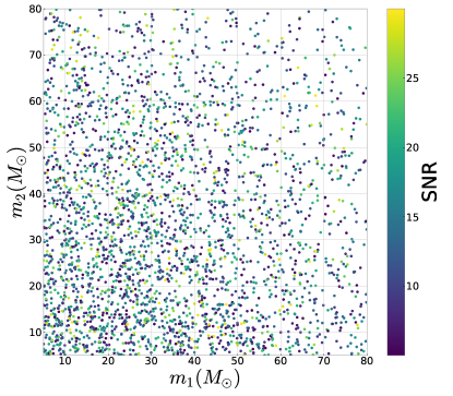
The simulated GW parameters are shown in Table 1. Note that the distance is a fixed value, but we rescale the simulated waveform to match SNR, which is randomly chosen in the range of . For the same SNR, the smaller-mass BBHs produce smaller strains, and thus they are difficult to be identified. In order to improve the ability of the network to identify signals within the insensitive ranges, we train the network with more low-mass signals (the number of is 5 times more than ). Meanwhile, for SNR, we also adopt the same treatment, we train the network with more low-SNR signals (the number of is 5 times more than ).
| Parameter | Uniform distribution |
|---|---|
| Component masses | |
| Right ascension | |
| Declination | |
| Polarization angle | |
| Luminosity distance | |
| Injection SNR |
II.2 U-Net architecture
The typical use of convolutional networks is on classification tasks, where the output of the image is a single class label. However, in many visual tasks, it is not enough to assign a single class label to an entire image. Instead, the desired output should include pixel-level localization, where a class label is assigned to each individual pixel. The U-Net algorithm can achieve this through semantic segmentation, which is an approach for identifying the class of an object for each pixel. The approach is particularly useful for tasks such as object detection, where the precise location and shape of the object of interest need to be identified.
The U-Net network is a convolutional neural network (CNN) originally developed for biomedical image segmentation Ronneberger et al. (2015). While based on CNN, it has undergone significant structural modifications. Unlike the standard CNN architecture, U-Net includes many feature channels in the upsampling part, allowing the network to propagate contextual information to higher resolution layers through a series of transpose convolutions. The main idea behind U-Net is to add successive layers to the traditional contracting network, replacing the convergence operation with an upsampling operation. This leads to an increase in output resolution, as these layers produce a U-shaped structure that is almost symmetric with the contracted part.
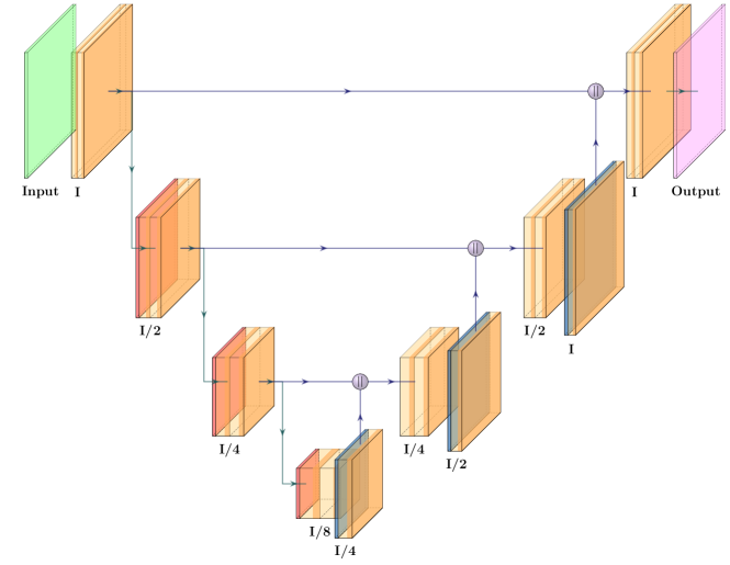
The network architecture is illustrated in Fig. 2. It consists of a contracted path (left side) and an extended path (right side). The contracting path follows the typical architecture of a convolutional network. It consists of the repeated application of two convolutions (unpadded convolutions), each followed by a rectified linear unit (ReLU) and a max pooling operation with stride 2 for downsampling. At each downsampling step, we double the number of feature channels. Every step in the expansive path consists of an upsampling of the feature map followed by a convolution (“up-convolution”) that halves the number of feature channels, a concatenation with the corresponding cropped feature map from the contracting path, and two convolutions, each followed by a ReLU. The cropping is necessary due to the loss of border pixels in every convolution. At the final layer, a convolution is used to map each 64-component feature vector to the desired number of classes. In total, the network has 23 convolutional layers.
II.3 Training
| Hyperparameter | Description | Prior value | Optimum value |
|---|---|---|---|
| learning rate for optimizer | |||
| weight decay for optimizer | |||
| initial number of convolution filters | 32 | ||
| batch size, i.e., number of samples per gradient descent step | 32,64 | 32 | |
| optimizer for training | Adam, NAdam | NAdam |
During the training process, the coefficients of the neural network are determined. To assign initial random values to the CNN parameters, we use the “Xavier” initialization, which is designed to keep the scale of gradients roughly the same in all layers. Then, we use the binary cross-entropy loss function to evaluate the deviation between the predicted values and the actual values in the training data.
The key component of CNN is the convolutional layer, which applies a set of filters to the input. The network consists of a series of stacked layers. In the first convolutional layer, we set the number of convolution kernels to 32. The kernel size determines the convolutional field of view and is fixed at . To maintain the output dimensionality, we employ the same padding method for both convolutions and transpose convolutions to handle sample boundaries. The stride determines the kernel traversal step size on the images. We use the default stride settings of 1 in convolutions and 2 in transpose convolutions.
Our selected U-Net architecture is trained end-to-end to the signal identification using the simulated data introduced in Sec. II.1. The details of the hyperparameters used in this work are listed in Table 2. The NAdam optimizer is used in the analysis with the default TensorFlow parameters. The hyperparameters are carefully fine-tuned to optimize the network Reddi et al. (2019). The batch size is optimized to 32 and the number of initial convolution filters is optimized to 32, both of which are limited by the GPU memory. The learning rate is set to , and weight decay is . We set dropout to be 0.2 and use batch normalization to make the mean and variance of the input data distribution of each layer in U-Net within a certain range. The total number of trainable parameters is . We apply a ReLU activation in every convolution. At last, we adopt the 200 epoch calculation scheme to improve our results.
At the end of every epoch, the performance of the network during the training is evaluated by average accuracy for the networks on each mini-batch. The training process is done within 6 hours on 4 NVIDIA GeForce RTX A6000 GPUs, each with 48 GB of memory.
| Name | Event type |
|---|---|
| GW170817 | BNS |
| GW190425 | BNS |
| GW190814 | NSBH |
| GW190917_114630 | NSBH |
| GW191219_163120 | NSBH |
| GW200105_162426 | NSBH |
| GW200115_042309 | NSBH |
| GW200210_092254 | NSBH |
III Results and discussion
III.1 Simulation results
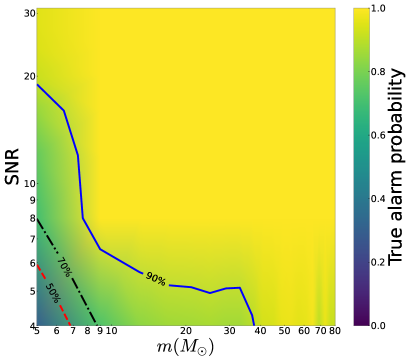
We first study the generalization ability of the network in GW detections considering the single mass and SNR. In the training dataset, we consider the equal-mass BBH mergers, the BH mass is sampled in the range of , and SNR is sampled in the range of . After 100 epochs of training, the accuracy of the test dataset is 90%. In order to show the generalization ability of the network, we show the results in Fig. 4 with and SNR in the ranges of and , respectively. We find that the network performs well in the high-mass and high-SNR regions, but not well in the low-mass and low-SNR regions. Therefore, for the lower-SNR region (), the network also performs not well. The prime cause is that the network is more effective for short signals. As the mass decreases, the longer signals are close to the characteristics of the random noise. In other words, at the same SNR, the short signals have stronger strains than those of the long signals. Therefore, it is easier to identify the short signals. Meanwhile, for the high-mass and low-SNR regions, the network performs better, which also means that the network has a certain generalization ability. Concretely, the network performs well when the single mass is higher than and SNR is greater than 8.
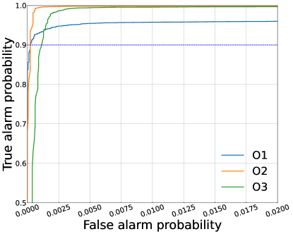
By training the network with the LIGO noise data in O1, O2, and O3, we use the test dataset for the final evaluation of the network. In Fig. 5, we show the receiver operating characteristic (ROC) curve, which illustrates the diagnostic ability of a binary classifier system Fawcett (2006). When the discrimination threshold changes, the ROC curve reflects the proportion of positive samples correctly identified (True alarm probability) versus the proportion of negative samples incorrectly identified (False alarm probability) Powers (2020). In this work, the true alarm probability threshold is set to 0.9. In addition, the false alarm probability of the network is better than 0.1%, which is comparable with the network in the recent literature Zhang et al. (2022); Barone et al. (2022); Verma et al. (2022).
III.2 Application to the real observations
We apply the trained network to the O1 and O2 data. In this subsection, we shall report the identification results. For each GW event, we identify the GW signals from LIGO Hanford and LIGO Livingston. Due to the low SNR of some GW signals, there will be missed detections during identification. Hence, we adopt the form of the union of LIGO Hanford and LIGO Livingston, i.e., we consider the signal identified as long as it is detected by either of the two detectors. Note that in the present work, we consider the identification of the GW signals from BBH mergers, so GW events involving NSs are not considered in this work.
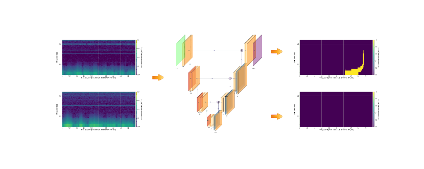
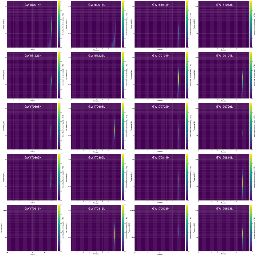
In Fig. 6, we show the time-frequency domain GW signals of O1 and O2 identified by the trained network. We could see that all the GW events are identified by the network. In fact, we also test the network by identifying BNS mergers and find that the network is unable to identify them, which is consistent with our expectations. From the figure, we could also see that the identified signals obtained from the network are also different for different GW events. The prime cause is that the time-frequency signals of GW for different chirp masses are different. The fact also means that the time-frequency domain GW signals identified by U-Net may be used to preliminarily determine the chirp masses of the GW sources. Previous work shows that the prior selection of the GW parameter has an important impact on the Bayesian inference Vitale et al. (2017). Our results show that the network could not only rapidly and accurately identify the GW signals, but also provide great help for the later Bayesian inferences.
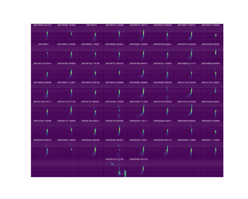
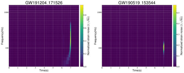
Subsequently, we apply the trained network to the identification of the O3 data. In Fig. 7, we show the time-frequency domain GW signals of O3 identified by the trained network. We could see that the trained network shows a strong ability to identify GW signals. Meanwhile, the identified ability of O3 is better than that of O2 because we use the background noise of O3 to train. 58 GW signals are clearly identified through the network. Note that for O3, we consider a total of 73 GW signals for analysis and only show the identified results. About 80% (79.3%) GW signals of O3 could be rapidly and accurately identified. In Fig. 8, we show the time-frequency GW signals of the GW191204171526 (chirp mass ) and GW190519153544 (chirp mass ) identified by the trained network. We could see that the lower-mass GW signals have a longer duration in the time-frequency domain, so they exhibit a shape similar to a “tail”. While the higher-mass GW signals have a shorter duration and therefore appear as a sharp peak. It also means that the trained network shows the potential of providing mass priors.
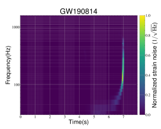
Our results show the potential of the U-Net algorithm in identifying time-frequency GW signals and providing mass priors in the future. In addition, we also use the trained network to identify BNS mergers, NSBH mergers, and some uncertain events. We find that our network could not identify BNS and NSBH mergers, which is also in line with our expectations. However, our network successfully identifies uncertain event GW190814 (the lightest BH or the heaviest NS) Abbott et al. (2020), which means that our network infers that it is a BBH merger event, as shown in Fig. 9.
IV Conclusion
In this work, we use the U-Net algorithm to identify time-frequency GW signals of LIGO O1, O2, and O3 observations. We trained the network using the dataset of pure background noise signals and the dataset of GW signal and background noise signal. In the test dataset, the false alarm probabilities for O1, O2, and O3 are all better than 0.1%. The trained network is then used to identify the real observations. The time-frequency domain GW signals of O1 and O2 are all identified. Moreover, due to the fact that the time-frequency domain GW signals for different chirp masses are different, the identified time-frequency domain GW signals by U-Net can be used to preliminarily determine the chirp masses of the GW sources. For O3, the trained network could identify about 80% GW events. Our results show that the U-Net algorithm could rapidly identify the time-frequency domain GW signals from BBH mergers and provide rapid prior information for the Bayesian inferences. In addition, the trained network infers GW190814 to be a BBH merger event.
Acknowledgements.
This research has made use of data or software obtained from the Gravitational Wave Open Science Center (gwosc.org), a service of LIGO Laboratory, the LIGO Scientific Collaboration, the Virgo Collaboration, and KAGRA. We thank He Wang for helpful discussions. This work was supported by the National Natural Science Foundation of China (Grants Nos. 11975072, 11875102, and 11835009) and the National SKA Program of China (Grants Nos. 2022SKA0110200 and 2022SKA0110203).References
- Abbott et al. (2016a) B. P. Abbott et al. (LIGO Scientific, Virgo), Phys. Rev. Lett. 116, 061102 (2016a), eprint 1602.03837.
- Einstein (1916) A. Einstein, Sitzungsberichte der Königlich Preußischen Akademie der Wissenschaften pp. 688–696 (1916).
- Abbott et al. (2017a) B. P. Abbott et al. (LIGO Scientific, Virgo), Phys. Rev. Lett. 119, 161101 (2017a), eprint 1710.05832.
- Abbott et al. (2017b) B. P. Abbott et al. (LIGO Scientific, Virgo, Fermi GBM, INTEGRAL, IceCube, AstroSat Cadmium Zinc Telluride Imager Team, IPN, Insight-Hxmt, ANTARES, Swift, AGILE Team, 1M2H Team, Dark Energy Camera GW-EM, DES, DLT40, GRAWITA, Fermi-LAT, ATCA, ASKAP, Las Cumbres Observatory Group, OzGrav, DWF (Deeper Wider Faster Program), AST3, CAASTRO, VINROUGE, MASTER, J-GEM, GROWTH, JAGWAR, CaltechNRAO, TTU-NRAO, NuSTAR, Pan-STARRS, MAXI Team, TZAC Consortium, KU, Nordic Optical Telescope, ePESSTO, GROND, Texas Tech University, SALT Group, TOROS, BOOTES, MWA, CALET, IKI-GW Follow-up, H.E.S.S., LOFAR, LWA, HAWC, Pierre Auger, ALMA, Euro VLBI Team, Pi of Sky, Chandra Team at McGill University, DFN, ATLAS Telescopes, High Time Resolution Universe Survey, RIMAS, RATIR, SKA South Africa/MeerKAT), Astrophys. J. Lett. 848, L12 (2017b), eprint 1710.05833.
- Aasi et al. (2015) J. Aasi et al. (LIGO Scientific), Class. Quant. Grav. 32, 074001 (2015), eprint 1411.4547.
- Acernese et al. (2015) F. Acernese et al. (VIRGO), Class. Quant. Grav. 32, 024001 (2015), eprint 1408.3978.
- Akutsu et al. (2019) T. Akutsu et al. (KAGRA), Nature Astron. 3, 35 (2019), eprint 1811.08079.
- (8) https://gwosc.org/eventapi/html/allevents/.
- Abbott et al. (2019a) B. P. Abbott et al. (LIGO Scientific, Virgo), Phys. Rev. X 9, 031040 (2019a), eprint 1811.12907.
- Abbott et al. (2021a) R. Abbott et al. (LIGO Scientific, Virgo), Phys. Rev. X 11, 021053 (2021a), eprint 2010.14527.
- Abbott et al. (2021b) R. Abbott et al. (LIGO Scientific, VIRGO, KAGRA) (2021b), eprint 2111.03606.
- Berti et al. (2015) E. Berti et al., Class. Quant. Grav. 32, 243001 (2015), eprint 1501.07274.
- Abbott et al. (2016b) B. P. Abbott et al. (LIGO Scientific, Virgo), Phys. Rev. Lett. 116, 221101 (2016b), [Erratum: Phys.Rev.Lett. 121, 129902 (2018)], eprint 1602.03841.
- Abbott et al. (2019b) B. P. Abbott et al. (LIGO Scientific, Virgo), Phys. Rev. Lett. 123, 011102 (2019b), eprint 1811.00364.
- Abbott et al. (2019c) B. P. Abbott et al. (LIGO Scientific, Virgo), Phys. Rev. D 100, 104036 (2019c), eprint 1903.04467.
- Abbott et al. (2021c) R. Abbott et al. (LIGO Scientific, Virgo), Phys. Rev. D 103, 122002 (2021c), eprint 2010.14529.
- Abbott et al. (2021d) R. Abbott et al. (LIGO Scientific, VIRGO, KAGRA) (2021d), eprint 2112.06861.
- Gong et al. (2022) C. Gong, T. Zhu, R. Niu, Q. Wu, J.-L. Cui, X. Zhang, W. Zhao, and A. Wang, Phys. Rev. D 105, 044034 (2022), eprint 2112.06446.
- Gong et al. (2023) C. Gong, T. Zhu, R. Niu, Q. Wu, J.-L. Cui, X. Zhang, W. Zhao, and A. Wang (2023), eprint 2302.05077.
- Mandel and Broekgaarden (2022) I. Mandel and F. S. Broekgaarden, Living Rev. Rel. 25, 1 (2022), eprint 2107.14239.
- van Son et al. (2022) L. A. C. van Son, S. E. de Mink, T. Callister, S. Justham, M. Renzo, T. Wagg, F. S. Broekgaarden, F. Kummer, R. Pakmor, and I. Mandel, Astrophys. J. 931, 17 (2022), eprint 2110.01634.
- Broekgaarden et al. (2021) F. S. Broekgaarden et al. (2021), eprint 2112.05763.
- Ezquiaga and Holz (2022) J. M. Ezquiaga and D. E. Holz, Phys. Rev. Lett. 129, 061102 (2022), eprint 2202.08240.
- Abbott et al. (2017c) B. P. Abbott et al. (LIGO Scientific, Virgo, 1M2H, Dark Energy Camera GW-E, DES, DLT40, Las Cumbres Observatory, VINROUGE, MASTER), Nature 551, 85 (2017c), eprint 1710.05835.
- Chen et al. (2018) H.-Y. Chen, M. Fishbach, and D. E. Holz, Nature 562, 545 (2018), eprint 1712.06531.
- Abbott et al. (2021e) R. Abbott et al. (LIGO Scientific, VIRGO, KAGRA) (2021e), eprint 2111.03604.
- Soares-Santos et al. (2019) M. Soares-Santos et al. (DES, LIGO Scientific, Virgo), Astrophys. J. Lett. 876, L7 (2019), eprint 1901.01540.
- Palmese et al. (2020) A. Palmese et al. (DES), Astrophys. J. Lett. 900, L33 (2020), eprint 2006.14961.
- Abbott et al. (2021f) B. P. Abbott et al. (LIGO Scientific, Virgo, VIRGO), Astrophys. J. 909, 218 (2021f), eprint 1908.06060.
- Holz and Hughes (2005) D. E. Holz and S. A. Hughes, Astrophys. J. 629, 15 (2005), eprint astro-ph/0504616.
- Dalal et al. (2006) N. Dalal, D. E. Holz, S. A. Hughes, and B. Jain, Phys. Rev. D 74, 063006 (2006), eprint astro-ph/0601275.
- Nissanke et al. (2010) S. Nissanke, D. E. Holz, S. A. Hughes, N. Dalal, and J. L. Sievers, Astrophys. J. 725, 496 (2010), eprint 0904.1017.
- Cutler and Holz (2009) C. Cutler and D. E. Holz, Phys. Rev. D 80, 104009 (2009), eprint 0906.3752.
- Camera and Nishizawa (2013) S. Camera and A. Nishizawa, Phys. Rev. Lett. 110, 151103 (2013), eprint 1303.5446.
- Vitale and Chen (2018) S. Vitale and H.-Y. Chen, Phys. Rev. Lett. 121, 021303 (2018), eprint 1804.07337.
- Bian et al. (2021) L. Bian et al., Sci. China Phys. Mech. Astron. 64, 120401 (2021), eprint 2106.10235.
- Cai and Yang (2017) R.-G. Cai and T. Yang, Phys. Rev. D 95, 044024 (2017), eprint 1608.08008.
- Cai et al. (2018a) R.-G. Cai, T.-B. Liu, X.-W. Liu, S.-J. Wang, and T. Yang, Phys. Rev. D 97, 103005 (2018a), eprint 1712.00952.
- Cai and Yang (2018) R.-G. Cai and T. Yang, EPJ Web Conf. 168, 01008 (2018), eprint 1709.00837.
- Zhang (2019) X. Zhang, Sci. China Phys. Mech. Astron. 62, 110431 (2019), eprint 1905.11122.
- Chen (2020) H.-Y. Chen, Phys. Rev. Lett. 125, 201301 (2020), eprint 2006.02779.
- Gray et al. (2020) R. Gray et al., Phys. Rev. D 101, 122001 (2020), eprint 1908.06050.
- Zhao et al. (2011) W. Zhao, C. Van Den Broeck, D. Baskaran, and T. G. F. Li, Phys. Rev. D 83, 023005 (2011), eprint 1009.0206.
- Zhao et al. (2018) W. Zhao, B. S. Wright, and B. Li, JCAP 10, 052 (2018), eprint 1804.03066.
- Jin et al. (2022a) S.-J. Jin, T.-N. Li, J.-F. Zhang, and X. Zhang (2022a), eprint 2202.11882.
- Du et al. (2019) M. Du, W. Yang, L. Xu, S. Pan, and D. F. Mota, Phys. Rev. D 100, 043535 (2019), eprint 1812.01440.
- Cai et al. (2018b) Y.-F. Cai, C. Li, E. N. Saridakis, and L. Xue, Phys. Rev. D 97, 103513 (2018b), eprint 1801.05827.
- Yang et al. (2020) W. Yang, S. Pan, E. Di Valentino, B. Wang, and A. Wang, JCAP 05, 050 (2020), eprint 1904.11980.
- Yang et al. (2019) W. Yang, S. Vagnozzi, E. Di Valentino, R. C. Nunes, S. Pan, and D. F. Mota, JCAP 07, 037 (2019), eprint 1905.08286.
- Bachega et al. (2020) R. R. A. Bachega, A. A. Costa, E. Abdalla, and K. S. F. Fornazier, JCAP 05, 021 (2020), eprint 1906.08909.
- Chang et al. (2019) Z. Chang, Q.-G. Huang, S. Wang, and Z.-C. Zhao, Eur. Phys. J. C 79, 177 (2019).
- Zhang et al. (2019) J.-F. Zhang, M. Zhang, S.-J. Jin, J.-Z. Qi, and X. Zhang, JCAP 09, 068 (2019), eprint 1907.03238.
- Mukherjee et al. (2021) S. Mukherjee, G. Lavaux, F. R. Bouchet, J. Jasche, B. D. Wandelt, S. M. Nissanke, F. Leclercq, and K. Hotokezaka, Astron. Astrophys. 646, A65 (2021), eprint 1909.08627.
- He (2019) J.-h. He, Phys. Rev. D 100, 023527 (2019), eprint 1903.11254.
- Zhao et al. (2020) Z.-W. Zhao, L.-F. Wang, J.-F. Zhang, and X. Zhang, Sci. Bull. 65, 1340 (2020), eprint 1912.11629.
- Wang et al. (2022) L.-F. Wang, S.-J. Jin, J.-F. Zhang, and X. Zhang, Sci. China Phys. Mech. Astron. 65, 210411 (2022), eprint 2101.11882.
- Qi et al. (2021) J.-Z. Qi, S.-J. Jin, X.-L. Fan, J.-F. Zhang, and X. Zhang, JCAP 12, 042 (2021), eprint 2102.01292.
- Jin et al. (2021) S.-J. Jin, L.-F. Wang, P.-J. Wu, J.-F. Zhang, and X. Zhang, Phys. Rev. D 104, 103507 (2021), eprint 2106.01859.
- Zhu et al. (2022) L.-G. Zhu, L.-H. Xie, Y.-M. Hu, S. Liu, E.-K. Li, N. R. Napolitano, B.-T. Tang, J.-d. Zhang, and J. Mei, Sci. China Phys. Mech. Astron. 65, 259811 (2022), eprint 2110.05224.
- de Souza et al. (2022) J. M. S. de Souza, R. Sturani, and J. Alcaniz, JCAP 03, 025 (2022), eprint 2110.13316.
- Jin et al. (2022b) S.-J. Jin, R.-Q. Zhu, L.-F. Wang, H.-L. Li, J.-F. Zhang, and X. Zhang, Commun. Theor. Phys. 74, 105404 (2022b), eprint 2204.04689.
- Cao et al. (2022) M.-D. Cao, J. Zheng, J.-Z. Qi, X. Zhang, and Z.-H. Zhu, Astrophys. J. 934, 108 (2022), eprint 2112.14564.
- Leandro et al. (2022) H. Leandro, V. Marra, and R. Sturani, Phys. Rev. D 105, 023523 (2022), eprint 2109.07537.
- Fu et al. (2021) X. Fu, L. Zhou, J. Yang, Z.-Y. Lu, Y. Yang, and G. Tang, Chin. Phys. C 45, 065104 (2021).
- Ye and Fishbach (2021) C. Ye and M. Fishbach, Phys. Rev. D 104, 043507 (2021), eprint 2103.14038.
- Chen et al. (2021) H.-Y. Chen, P. S. Cowperthwaite, B. D. Metzger, and E. Berger, Astrophys. J. Lett. 908, L4 (2021), eprint 2011.01211.
- Mitra et al. (2021) A. Mitra, J. Mifsud, D. F. Mota, and D. Parkinson, Mon. Not. Roy. Astron. Soc. 502, 5563 (2021), eprint 2010.00189.
- Hogg et al. (2020) N. B. Hogg, M. Martinelli, and S. Nesseris, JCAP 12, 019 (2020), eprint 2007.14335.
- Nunes (2020) R. C. Nunes, Phys. Rev. D 102, 024071 (2020), eprint 2007.07750.
- Borhanian et al. (2020) S. Borhanian, A. Dhani, A. Gupta, K. G. Arun, and B. S. Sathyaprakash, Astrophys. J. Lett. 905, L28 (2020), eprint 2007.02883.
- Jin et al. (2020) S.-J. Jin, D.-Z. He, Y. Xu, J.-F. Zhang, and X. Zhang, JCAP 03, 051 (2020), eprint 2001.05393.
- Yu et al. (2020) J. Yu, Y. Wang, W. Zhao, and Y. Lu, Mon. Not. Roy. Astron. Soc. 498, 1786 (2020), eprint 2003.06586.
- Jin et al. (2023) S.-J. Jin, S.-S. Xing, Y. Shao, J.-F. Zhang, and X. Zhang, Chin. Phys. C 47, 065104 (2023), eprint 2301.06722.
- Abbott et al. (2019d) B. P. Abbott et al. (LIGO Scientific, Virgo), Phys. Rev. D 100, 064064 (2019d), eprint 1906.08000.
- LeCun et al. (2015) Y. LeCun, Y. Bengio, and G. Hinton, nature 521, 436 (2015).
- Guest et al. (2018a) D. Guest, K. Cranmer, and D. Whiteson, Annual Review of Nuclear and Particle Science 68, 161 (2018a).
- Baldi et al. (2014) P. Baldi, P. Sadowski, and D. Whiteson, Nature Commun. 5, 4308 (2014), eprint 1402.4735.
- Guest et al. (2018b) D. Guest, K. Cranmer, and D. Whiteson, Ann. Rev. Nucl. Part. Sci. 68, 161 (2018b), eprint 1806.11484.
- Wei and Huerta (2020) W. Wei and E. A. Huerta, Phys. Lett. B 800, 135081 (2020), eprint 1901.00869.
- George et al. (2017) D. George, H. Shen, and E. A. Huerta (2017), eprint 1706.07446.
- Chatterjee et al. (2019) C. Chatterjee, L. Wen, K. Vinsen, M. Kovalam, and A. Datta, Phys. Rev. D 100, 103025 (2019), eprint 1909.06367.
- Shen et al. (2019) H. Shen, D. George, E. A. Huerta, and Z. Zhao (2019), eprint 1903.03105.
- Cuoco et al. (2021) E. Cuoco et al., Mach. Learn. Sci. Tech. 2, 011002 (2021), eprint 2005.03745.
- Álvares et al. (2020) J. a. D. Álvares, J. A. Font, F. F. Freitas, O. G. Freitas, A. P. Morais, S. Nunes, A. Onofre, and A. Torres-Forné (2020), eprint 2011.10425.
- Green et al. (2020) S. R. Green, C. Simpson, and J. Gair, Phys. Rev. D 102, 104057 (2020), eprint 2002.07656.
- Green and Gair (2021) S. R. Green and J. Gair, Mach. Learn. Sci. Tech. 2, 03LT01 (2021), eprint 2008.03312.
- Dax et al. (2023) M. Dax, S. R. Green, J. Gair, M. Pürrer, J. Wildberger, J. H. Macke, A. Buonanno, and B. Schölkopf, Phys. Rev. Lett. 130, 171403 (2023), eprint 2210.05686.
- Marulanda et al. (2020) J. P. Marulanda, C. Santa, and A. E. Romano, Phys. Lett. B 810, 135790 (2020), eprint 2004.01050.
- Singh et al. (2021) S. Singh, A. Singh, A. Prajapati, and K. N. Pathak, Mon. Not. Roy. Astron. Soc. 508, 1358 (2021), eprint 2008.06550.
- Mould et al. (2022) M. Mould, D. Gerosa, and S. R. Taylor, Phys. Rev. D 106, 103013 (2022), eprint 2203.03651.
- Chatterjee et al. (2021) C. Chatterjee, L. Wen, F. Diakogiannis, and K. Vinsen, Phys. Rev. D 104, 064046 (2021), eprint 2105.03073.
- McLeod et al. (2022) A. McLeod, D. Jacobs, C. Chatterjee, L. Wen, and F. Panther (2022), eprint 2201.11126.
- Langendorff et al. (2023) J. Langendorff, A. Kolmus, J. Janquart, and C. Van Den Broeck, Phys. Rev. Lett. 130, 171402 (2023), eprint 2211.15097.
- Chatterjee et al. (2022) C. Chatterjee, L. Wen, D. Beveridge, F. Diakogiannis, and K. Vinsen (2022), eprint 2207.14522.
- George and Huerta (2018a) D. George and E. A. Huerta, Phys. Rev. D 97, 044039 (2018a), eprint 1701.00008.
- Gabbard et al. (2018) H. Gabbard, M. Williams, F. Hayes, and C. Messenger, Phys. Rev. Lett. 120, 141103 (2018), eprint 1712.06041.
- Krastev et al. (2021) P. G. Krastev, K. Gill, V. A. Villar, and E. Berger, Phys. Lett. B 815, 136161 (2021), eprint 2012.13101.
- Cabero et al. (2020) M. Cabero, A. Mahabal, and J. McIver, Astrophys. J. Lett. 904, L9 (2020), eprint 2010.11829.
- Jadhav et al. (2021) S. Jadhav, N. Mukund, B. Gadre, S. Mitra, and S. Abraham, Phys. Rev. D 104, 064051 (2021), eprint 2010.08584.
- Xia et al. (2021) H. Xia, L. Shao, J. Zhao, and Z. Cao, Phys. Rev. D 103, 024040 (2021), eprint 2011.04418.
- George and Huerta (2018b) D. George and E. A. Huerta, Phys. Lett. B 778, 64 (2018b), eprint 1711.03121.
- Fan et al. (2019) X. Fan, J. Li, X. Li, Y. Zhong, and J. Cao, Sci. China Phys. Mech. Astron. 62, 969512 (2019), eprint 1811.01380.
- 1909.13442 et al. (2020) 1909.13442, S. Wu, Z. Cao, X. Liu, and J.-Y. Zhu, Phys. Rev. D 101, 104003 (2020), eprint 1909.13442.
- Krastev (2020) P. G. Krastev, Phys. Lett. B 803, 135330 (2020), eprint 1908.03151.
- Wei et al. (2021) W. Wei, A. Khan, E. A. Huerta, X. Huang, and M. Tian, Phys. Lett. B 812, 136029 (2021), eprint 2010.15845.
- Verma et al. (2022) C. Verma, A. Reza, D. Krishnaswamy, S. Caudill, and G. Gaur, AIP Conf. Proc. 2555, 020010 (2022), eprint 2110.01883.
- Moreno et al. (2022) E. A. Moreno, B. Borzyszkowski, M. Pierini, J.-R. Vlimant, and M. Spiropulu, Mach. Learn. Sci. Tech. 3, 025001 (2022), eprint 2107.12698.
- Zhang et al. (2022) Y. Zhang, H. Xu, M. Liu, C. Liu, Y. Zhao, and J. Zhu, Phys. Rev. D 106, 122002 (2022).
- Qiu et al. (2023) R. Qiu, P. G. Krastev, K. Gill, and E. Berger, Phys. Lett. B 840, 137850 (2023), eprint 2210.15888.
- Nousi et al. (2022) P. Nousi, A. E. Koloniari, N. Passalis, P. Iosif, N. Stergioulas, and A. Tefas (2022), eprint 2211.01520.
- Ma et al. (2022) C. Ma, W. Wang, H. Wang, and Z. Cao, Phys. Rev. D 105, 083013 (2022), eprint 2204.12058.
- Marianer et al. (2020) T. Marianer, D. Poznanski, and J. X. Prochaska, Mon. Not. Roy. Astron. Soc. 500, 5408 (2020), eprint 2010.11949.
- Boudart and Fays (2022) V. Boudart and M. Fays, Phys. Rev. D 105, 083007 (2022), eprint 2201.08727.
- Ravichandran et al. (2023) A. Ravichandran, A. Vijaykumar, S. J. Kapadia, and P. Kumar (2023), eprint 2302.00666.
- Ronneberger et al. (2015) O. Ronneberger, P. Fischer, and T. Brox, in Medical Image Computing and Computer-Assisted Intervention–MICCAI 2015: 18th International Conference, Munich, Germany, October 5-9, 2015, Proceedings, Part III 18 (Springer, 2015), pp. 234–241.
- Gao et al. (2022) L.-Y. Gao, Y. Li, S. Ni, and X. Zhang (2022), eprint 2212.08773.
- Ni et al. (2022) S. Ni, Y. Li, L.-Y. Gao, and X. Zhang, Astrophys. J. 934, 83 (2022), eprint 2204.02780.
- Devine et al. (2016) C. Devine, Z. B. Etienne, and S. T. McWilliams, Class. Quant. Grav. 33, 125025 (2016), eprint 1601.03393.
- Bohé et al. (2017) A. Bohé et al., Phys. Rev. D 95, 044028 (2017), eprint 1611.03703.
- Nitz et al. (2023) A. Nitz, I. Harry, D. Brown, C. M. Biwer, J. Willis, T. D. Canton, C. Capano, T. Dent, L. Pekowsky, S. De, et al., gwastro/pycbc: v2.1.2 release of pycbc (2023), URL https://doi.org/10.5281/zenodo.7885796.
- (121) https://github.com/HarisIqbal88/PlotNeuralNet.
- Reddi et al. (2019) S. J. Reddi, S. Kale, and S. Kumar, arXiv preprint arXiv:1904.09237 (2019).
- Fawcett (2006) T. Fawcett, Pattern recognition letters 27, 861 (2006).
- Powers (2020) D. M. Powers, arXiv preprint arXiv:2010.16061 (2020).
- Barone et al. (2022) F. P. Barone, D. Dell’Aquila, and M. Russo (2022), eprint 2206.06004.
- Vitale et al. (2017) S. Vitale, D. Gerosa, C.-J. Haster, K. Chatziioannou, and A. Zimmerman, Phys. Rev. Lett. 119, 251103 (2017), eprint 1707.04637.
- Abbott et al. (2020) R. Abbott et al. (LIGO Scientific, Virgo), Astrophys. J. Lett. 896, L44 (2020), eprint 2006.12611.