Sharp high-probability sample complexities for policy evaluation
with linear function approximation

Abstract

This paper is concerned with the problem of policy evaluation with linear function approximation in discounted infinite horizon Markov decision processes. We investigate the sample complexities required to guarantee a predefined estimation error of the best linear coefficients for two widely-used policy evaluation algorithms: the temporal difference (TD) learning algorithm and the two-timescale linear TD with gradient correction (TDC) algorithm. In both the on-policy setting, where observations are generated from the target policy, and the off-policy setting, where samples are drawn from a behavior policy potentially different from the target policy, we establish the first sample complexity bound with high-probability convergence guarantee that attains the optimal dependence on the tolerance level. We also exhihit an explicit dependence on problem-related quantities, and show in the on-policy setting that our upper bound matches the minimax lower bound on crucial problem parameters, including the choice of the feature map and the problem dimension.

Keywords: policy evaluation, temporal difference learning, two-timescale stochastic approximation, minimax optimal, function approximation

1 Introduction

Policy evaluation plays a critical role in many scientific and engineering applications in which practitioners aim to evaluate the performance of a target strategy based on either sequentially collected or a batch of offline data samples (Murphy,, 2003; Bojinov and Shephard,, 2019; Tang and Wiens,, 2021; Dann et al.,, 2014). For example, in clinical trials (Tang and Wiens,, 2021), real-time data acquisition might be expensive and risky; it is thus of essential value if historical data can be analyzed and information can be transferred to new tasks. While in other applications, such as mobile health (Bertsimas et al.,, 2022), it is practical to implement the desired policy and collect its feedback in a timely manner.

Mathematically, Markov decision processes (MDPs) provide a general framework to design policy evaluation methods in dynamic settings; reinforcement learning (RL) is often modeled using MDPs when the exact model configuration is not available (Sutton and Barto,, 2018; Bertsekas,, 2017). In this framework, a target policy is assessed through its corresponding value function. In practice, evaluating value functions often require an overwhelming number of samples due to the large dimensionality of the underlying state space. For this reason, RL methods are normally concerned with some form of function approximation. Dating back to the seminal work of Tsitsiklis and Van Roy, (1997), there has been an extensive line of works that consider different types of function approximation, including linear function approximation (Bhandari et al.,, 2021; Fan et al.,, 2020), reproducing kernel Hilbert space (Farahmand et al.,, 2016; Duan et al.,, 2021), deep neural networks (Bertsekas and Tsitsiklis,, 1995; Arulkumaran et al.,, 2017) or function approximation on the model itself (see, e.g. Jin et al., (2020); Wang et al., 2021a ; Li et al., 2021a ), with a focus on improving the sample efficiency of RL algorithms.

Two settings: on-policy vs. off-policy.

The main goal of this paper is to provide sharp statistical guarantees of policy evaluation algorithms with linear function approximation in two different settings. As the aforementioned examples already indicated, there are typically two different types of data-generating mechanisms to consider: the on-policy setting when we have access to the outcomes of the target policy and the off-policy setting, in which the only available data are generated from a behavior policy that is potentially different from the target policy.

In the on-policy setting, temporal difference (TD) learning is arguably the most popular algorithm (Sutton,, 1988) for policy evaluation in RL practice, partly because it is easy to implement and lends itself well to function approximations. As a model-free algorithm, TD learning processes data in an online manner without explicitly modeling the environment and is, therefore, memory efficient. While the asymptotic convergence of TD with linear function approximation has been known since Tsitsiklis and Van Roy, (1997), the finite-sample minimax optimality of TD has been established only recently for the tabular MDP (Li et al., 2023a, ). For TD learning with linear function approximation, several recent contributions have produced new non-asymptotic analyses and insights (e.g. Bhandari et al., (2021); Dalal et al., 2018a ; Srikant and Ying, (2019); Lakshminarayanan and Szepesvari, (2018)), which partially unveil impacts of both the tolerance level and various problem-related parameters on its sample efficiency. However, minimax-optimal dependence on the tolerance level (i.e. target level of estimation accuracy) is only established in expectation instead of with high probability; furthermore, the optimal dependence on problem-related parameters, such as the size of the state space and the effective horizon, still remains unsettled, and it is unclear whether existing sample complexity bounds can be further improved. Failing to understand these questions, however, casts doubt on whether TD with linear function approximation is statistically efficient in practice, and brings difficulties to performing statistical inference based on TD estimators. In this paper, we seek to answer these questions by providing tighter characterizations of the performance of TD with linear function approximation.

In the off-policy setting, it is known that the error of TD learning with linear function approximation may diverge to infinity (Baird,, 1995). In order to address this issue, Sutton et al., (2009) proposed a now popular alternative with two-timescale learning rates, called the linear TD with gradient correction (TDC) algorithm, which enjoys convergence guarantees in the off-policy case. In terms of finite-sample guarantees, although a number of recent efforts (see, e.g. Dalal et al., 2018b ; Xu and Liang, (2021); Wang et al., 2021b ; Dalal et al., (2020); Kaledin et al., (2020); Gupta et al., (2019)) tried to characterize the statistical performance of TDC for both $i.i.d.$ and Markovian data, they remain inadequate in providing either a convergence guarantee with high-probability, an explicit dependence on salient problem parameters, or a sharp dependence on the sample size. The challenge lies in dealing with the statistical dependence between two separate iterate sequences at different timescales. To tackle this challenge, it calls for a new analysis framework for the TDC algorithm.

1.1 Our main contributions

This paper is concerned with evaluating the performance of a given target policy $\pi$ in an infinite-horizon $\gamma$-discounted MDP with a finite but large number of states. The goal is to learn the best linear approximation of the value function in a pre-specified feature space given $i.i.d.$ transition pairs drawn from the stationary distribution. In the on-policy setting, we focus on the TD learning algorithm; in the off-policy setting, we shift gear to the TDC learning algorithm. We summarize our main contributions as follows, with their exact statements and consequences postponed to later sections.

• Via a careful analysis of TD learning with Polyak-Ruppert averaging, we show that, in the on-policy setting, a number of samples of order

  $$\widetilde{O}\left(\frac{\max_{s}\{\bm{\phi}(s)^{\top}\bm{\Sigma}^{-1}\bm{\phi}(s)\}(1+\|\bm{\theta}^{\star}\|_{\bm{\Sigma}}^{2})}{(1-\gamma)^{2}\varepsilon^{2}}\right)$$

  is sufficient to achieve an accuracy level (estimation error) of $\varepsilon>0$, with high probability. Here, $\bm{\phi}(s)\in{}^{d}$ indicates the linear feature vector for the state $s$ in the state space $\mathcal{S}$, $\bm{\theta}^{\star}$ is the best linear approximation coefficient of the value function, and $\bm{\Sigma}$ corresponds to the feature covariance matrix weighted by the stationary distribution. See Section 2 for the definitions of these parameters. Compared to prior work by Bhandari et al., (2021) and  Srikant and Ying, (2019), our sample complexity bound can be tighter by a factor of $\mathsf{cond}(\bm{\Sigma})$ which can be as large as $|\mathcal{S}|$ (the cardinality of the state space). Our result is also the first to control $\varepsilon$-convergence with high probability that matches the minimax-optimal dependence on the tolerance level $\varepsilon$. To assess the tightness of this upper bound, we provide a minimax lower bound in Section 3.3, which certifies the optimal dependence of our bound on both the tolerance level $\varepsilon$ and problem-related parameters $\bm{\Sigma}$ and $\bm{\theta}^{\star}$.

• In the off-policy setting, we establish a sample complexity bound for the TDC algorithm of order

  $$\widetilde{O}\left(\frac{\rho_{\max}^{7}}{\lambda_{1}^{4}\lambda_{2}^{3}}\frac{\|\widetilde{\bm{\Sigma}}\|^{2}}{\varepsilon^{2}}(1+\|\widetilde{\bm{\theta}}^{\star}\|_{\widetilde{\bm{\Sigma}}}^{2})\right),$$

  where $\widetilde{\bm{\theta}}$ corresponds to the best linear approximation coefficient of the value function in the off-policy setting, $\widetilde{\bm{\Sigma}}$ is the feature covariance matrix under the behavior policy, $\rho_{\max}$ denotes the largest importance sampling ratio measuring the discrepancy between the target policy and the behavior policy, and lastly, $\lambda_{1}$ and $\lambda_{2}$ denote the smallest eigenvalues of some problem-dependent matrices. Details about these constants are deferred to Section 4. To the best of our knowledge, our bound is the first one to control $\varepsilon$-convergence with high probability that matches the minimax-optimal dependence on the tolerance level $\varepsilon$. At the same time, our sample complexity bound also provides an explicit dependence on the salient parameters.

Comparisons of our results to existing bounds and relevant commentary can be found in Table 1 and  2.

paper	algorithm	stepsize	sample complexity	error control
Bhandari et al., (2021)	TD	$\eta_{t}\asymp t^{-1}$	$O\left(\frac{\|\bm{\Sigma}^{-2}\|\|\bm{\Sigma}\|\|\bm{\theta}^{\star}\|_{\bm{\Sigma}}^{2}}{(1-\gamma)^{2}\varepsilon^{2}}\right)$	in expectation
Srikant and Ying, (2019)	TD	$\eta_{t}\asymp T^{-1}$	$O\left(\frac{\|\bm{\Sigma}^{-2}\|\|\bm{\Sigma}\|\|\bm{\theta}^{\star}\|_{\bm{\Sigma}}^{2}}{(1-\gamma)^{2}\varepsilon^{2}}\right)$	in expectation
Dalal et al., 2018a	TD	$\eta_{t}=t^{-1}$	$O\left(\frac{1}{\varepsilon^{\max\{2,1+\frac{1}{\lambda}\}}}\right)$	w. high-prob
This work	Averaged TD	$\eta_{t}=\eta$	$O\left(\frac{\|\bm{\Sigma}^{-1}\|\|\bm{\theta}^{\star}\|_{\bm{\Sigma}}^{2}}{(1-\gamma)^{2}\varepsilon^{2}}\right)$	w. high-prob

Table 1: Comparisons with prior results (up to logarithmic terms) in finding an $\varepsilon$-optimal solution using TD learning. Using the Polyak-Ruppert averaging, our result improves upon previous sample complexity bounds by a multiplicative factor of the condition number of $\bm{\Sigma}$, and is the first sample complexity with high-probability guarantee of convergence to match the minimax-optimal dependence on the tolerance level $\varepsilon$.

1.2 Other related works

In this section, we review several recent lines of works and provide a broader context of the current paper.

Finite-sample guarantees for policy evaluation.

Classical analyses of policy evaluation algorithms have mainly focused on providing asymptotic guarantees given a fixed model (Tsitsiklis and Van Roy,, 1997; Szepesvári,, 1998). New tools developed in high-dimensional statistics and probability allow for a fine-grained understanding of these algorithms especially from a finite-sample and finite-time perspective. As argued in this paper, understanding how statistical errors depend on the effective horizon, dimension of the problem and the number of samples, is essential as it provides important insights on how these RL algorithms perform in practice. A highly incomplete list of prior art includes Khamaru et al., (2020); Jin et al., (2018); Srikant and Ying, (2019); Bhandari et al., (2021); Dalal et al., 2018a ; Lakshminarayanan and Szepesvari, (2018); Boyan, (1999) with a focus on the non-asymptotic analyses for model-free algorithms, and Sidford et al., (2018); Agarwal et al., (2020); Pananjady and Wainwright, (2021); Li et al., 2023b which derive non-asymptotic bounds for model-based algorithms.

Stochastic approximation.

The idea of stochastic approximation (SA) (Lai,, 2003; Robbins and Monro,, 1951) lies at the core of the TD and TDC learning algorithms considered in this paper. With the intention of solving a deterministic fixed-point equation, SA methods perform stochastic updates based on approximations of the current residual. The asymptotic theory of SA methods are relatively well-developed, where SA iterates provably track the trajectory of a limiting ordinary differential equation (Borkar,, 2009; Borkar and Meyn,, 2000) and with properly decaying step sizes, the Polyak-Ruppert averaged iterates asymptotically follow the central limit theorem. Recently, non-asymptotic results have also been obtained for SA for different problems especially in the RL setting; see Mou et al., (2020); Moulines and Bach, (2011); Lakshminarayanan and Szepesvari, (2018); Nemirovski et al., (2009) and references therein. The TDC algorithm is a special case of two-timescale linear SA, whose convergence rates have also been investigated in Dalal et al., (2020); Xu et al., (2019); Wu et al., (2020); Gupta et al., (2019), among others.

Off-policy learning.

Policy evaluation in the off-policy setting is closely related to offline or batch RL, which aims to learn purely based on historical data without actively exploring the environment. The main challenge here lies in the discrepancy between the behavior policy and the target or optimal policy. One natural approach is to use importance sampling (IS) in order to form an unbiased estimator of the target policy (Precup,, 2000), and various different techniques have been applied to reduce the high variance of IS (see, e.g. Jiang and Li, (2016); Ma et al., (2022); Thomas and Brunskill, (2016); Xie et al., (2019); Kallus and Uehara, (2020); Yang et al., (2020)). Non-asymptotic guarantees are also provided for off-policy evaluation using a fitted $Q$-iteration approach under linear function approximation in Duan et al., (2020). A recent line of works also considered finding the optimal policy using batch datasets (Jin et al.,, 2021; Xie et al.,, 2021; Li et al.,, 2022; Shi et al.,, 2022; Rashidinejad et al.,, 2021).

paper	algorithm	stepsize	sample complexity	error control
Dalal et al., (2020)	Projected TDC	$\alpha_{t}=t^{-\alpha}$, $\beta_{t}=t^{-\beta}$	$O\left(\frac{1}{\varepsilon^{2\alpha}}\right),\alpha<1$	w. high-prob
Kaledin et al., (2020)	TDC	$\alpha_{t},\beta_{t}\asymp\frac{1}{T}$	$O\left(\frac{1}{\varepsilon^{2}}\right)$	in expectation
Xu and Liang, (2021)	Batched TDC	$\alpha_{t}=\alpha$, $\beta_{t}=\beta$	$O\left(\frac{1}{\varepsilon^{2}}\log\frac{1}{\varepsilon}\right)$	in expectation
This work	TDC	$\alpha_{t},\beta_{t}\asymp\frac{1}{T}$	$O\left(\frac{1}{\varepsilon^{2}}\right)$	w. high-prob

Table 2: Comparisons with prior results (up to logarithmic terms) in finding an $\varepsilon$-optimal solution using TDC learning. We omit dependence on problem-related parameters in this table. Our sample complexity bound for TDC is the first to achieve high-probability convergence guarantee with non-varying stepsizes and without using projection steps or batched updates; in the mean time, we also provide explicit dependence on problem-related parameters.

1.3 Notation

Throughout this paper, we denote by $\Delta(\mathcal{S})$ (resp. $\Delta(\mathcal{A})$) the probability simplex over the finite set $\mathcal{S}$ (resp. $\mathcal{A}$). For any positive integer $n$, we use $[n]$ to denote the set of positive integers that are no larger than $n$: $[n]=\{1,2,...,n\}$. When a function is applied to a vector, it should be understood as being applied in a component-wise fashion; for example, $\sqrt{\bm{z}}:=[\sqrt{z_{i}}]_{1\leq i\leq n}$ and $|\bm{z}|:=[|z_{i}|]_{1\leq i\leq n}$. For any vectors $\bm{z}=[a_{i}]_{1\leq i\leq n}$ and $\bm{w}=[w_{i}]_{1\leq i\leq n}$, the notation $\bm{z}\geq\bm{w}$ (resp. $\bm{z}\leq\bm{w}$) stands for $z_{i}\geq w_{i}$ (resp. $z_{i}\leq w_{i}$) for all $1\leq i\leq n$. Additionally, we write $\bm{1}$ for the all-one vector, $\bm{I}$ for the identity matrix, and $\mathds{1}\{\cdot\}$ for the indicator function.

For any matrix $\bm{P}=[P_{ij}]$, we denote $\|\bm{P}\|_{1}:=\max_{i}\sum_{j}|P_{ij}|$. Given a symmetric positive definite matrix $\bm{D}$, define the inner product $\langle\cdot,\cdot\rangle_{\bm{D}}$ as $\langle\bm{u},\bm{v}\rangle_{\bm{D}}=\bm{u}^{\top}\bm{D}\bm{v}$ and the associated norm $\|\bm{v}\|_{\bm{D}}=\sqrt{\langle\bm{v},\bm{v}\rangle_{\bm{D}}}$. For any matrix $\bm{M}$, we use $\|\bm{M}\|$ to denote its operator norm (i.e. the largest singular value), if not specified otherwise. Throughout this paper, we use $c,c_{0},c_{1},C,\cdots$ to denote universal constants that do not depend either on the parameters of the MDP or the target levels $(\varepsilon,\delta)$; their exact values may change from line to line. Given two sequences, $\{f_{t}\}_{t\geq 0}$ and $\{g_{t}\}_{t\geq 0}$, we write $f_{t}\lesssim g_{t}$ (resp. $f_{t}\gtrsim g_{t}$) or $f_{t}=O(g_{t})$ (resp. $g_{t}=O(f_{t})$) if there exists some universal constant $c_{1}>0$, such that $f_{t}\leq c_{1}g_{t}$ (resp. $f\geq c_{1}g$). If both $f=O(g)$ and $g=O(f)$ hold simultaneously, we write $f_{t}\asymp g_{t}$ or $f_{t}=\Theta(g_{t}).$ We adopt the notation $f=\widetilde{O}(g)$ to indicate $f=O(g)$ up to logarithmic factors in $g$. For any symmetric matrix $\bm{X}$, we use $\lambda_{\min}(\bm{X})$ to denote its smallest eigenvalue.

2 Problem formulation

2.1 Model and settings

Markov decision process.

Consider an infinite-horizon MDP $\mathcal{M}=(\mathcal{S},\mathcal{A},\mathcal{P},r,\gamma)$ with discounted rewards, where $\mathcal{S}$ and $\mathcal{A}$ denote respectively the (finite) state space and action space, and $\gamma\in(0,1)$ indicates the discount factor (Bertsekas,, 2017). The probability transition kernel of the MDP is given by $\mathcal{P}:\mathcal{S}\times\mathcal{A}\mapsto\Delta(\mathcal{S})$, where for each state-action pair $(s,a)\in\mathcal{S}\times\mathcal{A}$, $\mathcal{P}(\cdot\mid{s,a})\in\Delta(\mathcal{S})$ denotes the transition probability distribution from state $s$ when action $a$ is executed. The reward function is represented by the function $r:\mathcal{S}\times\mathcal{A}\mapsto[0,1]$, where $r(s,a)$ denotes the immediate reward from state $s$ when action $a$ is taken; for simplicity, we assume throughout that all immediate rewards lie within $[0,1]$.

A policy $\pi:\mathcal{S}\mapsto\Delta(\mathcal{A})$ is an action selection rule that maps a state to a distribution over the set of actions; in particular, it is said to be stationary if it is time-invariant. The value function $V^{\pi}:\mathcal{S}\mapsto\mathbb{R}$ is used to measure the quality of a policy $\pi$, defined as

$$\forall s\in\mathcal{S}:\qquad V^{\pi}(s)\coloneqq\mathbb{E}\left[\sum_{t=0}^{\infty}\gamma^{t}r(s_{t},a_{t})\,\big{|}\,s_{0}=s\right],$$ (1)

which is the expected discounted cumulative reward received by following the policy $\pi$ under the MDP $\mathcal{M}$ when initialized at state $s_{0}=s$. Here, $a_{t}\sim\pi(\cdot\mid s_{t})$ and $s_{t+1}\sim\mathcal{P}(\cdot\mid s_{t},a_{t})$ for all $t\geq 0$. It can be easily verified that $0\leq V^{\pi}(s)\leq\frac{1}{1-\gamma}$ for any $\pi$.

For a given policy $\pi$, we can define the reward function of every state $s\in\mathcal{S}$ as the expected reward for $(s,a)$ when $a$ is chosen according to $\pi$:

$$r(s)=\mathbb{E}_{a\sim\pi(\cdot|s)}[r(s,a)].$$ (2)

For simplicity, we introduce the vector notation for the reward function $\bm{r}:=[r(s)]_{1\leq s\leq|\mathcal{S}|}\in\mathbb{R}^{|\mathcal{S}|}$, and the value function $\bm{V}^{\pi}=[V^{\pi}(s)]_{1\leq s\leq|\mathcal{S}|}\in\mathbb{R}^{|\mathcal{S}|}$. We can also define the transition matrix $\bm{P}^{\pi}$ for this given policy $\pi$, such that its $(i,j)$ element represents the probability that state $i$ is transited to state $j$ under the policy $\pi$; formally,

$${P}^{\pi}_{ij}=\sum_{a\in\mathcal{A}}\mathcal{P}(s_{t+1}=j\mid s_{t}=i,a_{t}=a)\pi(a_{t}=a\mid s_{t}=i).$$ (3)

We denote by $\mu$ the stationary distribution corresponding to the Markov chain when the transition follows $\bm{P}^{\pi}$, which we assume to be well-defined, and introduce the vector notation $\bm{\mu}:=[\mu(s)]_{1\leq s\leq|\mathcal{S}|}\in\mathbb{R}^{|\mathcal{S}|}$.

Linear approximation for the value function.

As discussed previously, it is often infeasible to collect a number of samples that scales with the ambient dimension $|\mathcal{S}|$. This motivates the search for lower dimension approximation of the value function, of which linear approximation emerges as a convenient option. Mathematically, for ${\bm{\theta}}\in{}^{d}$, define $V_{\bm{\theta}}(s)$ as

$$\forall s\in\mathcal{S}:\qquad V_{\bm{\theta}}(s)={\bm{\phi}}(s)^{\top}{\bm{\theta}},$$

where $\bm{\phi}(s)\in\mathbb{R}^{d}$ is the feature vector associated with state $s\in\mathcal{S}$, with $d\leq|\mathcal{S}|$. The vector ${\bm{\theta}}$ of linear coefficients is shared across states.

Using matrix notation, we let

$$\bm{\Phi}:=\left[\bm{\phi}(1),\bm{\phi}(2),\cdots,\bm{\phi}(|\mathcal{S}|)\right]^{\top}\in\mathbb{R}^{|\mathcal{S}|\times d},$$ (4)

be the feature matrix that concatenates the feature vectors for all states and ${\bm{V}}_{\theta}=[V_{\bm{\theta}}(s)]_{s\in\mathcal{S}}\in{}^{|S|}$ be the linear approximation vector to the value function. It follows that

$${\bm{V}}_{\theta}=\bm{\Phi}\bm{\theta}.$$

We impose the following mild assumption on the feature vectors.

Assumption 1.

The columns of $\bm{\Phi}$ are linearly independent with Euclidean norm uniformly bounded by one, i.e. $\max_{s\in\mathcal{S}}\|\bm{\phi}(s)\|_{2}\leq 1$.

2.2 Policy evaluation with linear approximation

On-policy evaluation with linear approximation.

The task of policy evaluation is to measure the value function $V^{\pi}(s)$ for every $s\in\mathcal{S}$ (see definition (1)) given a policy $\pi$ of interest. In the on-policy setting, data samples are collected while the policy $\pi$ is executed and a sequence of samples are obtained

$$\{(s_{0},a_{0},r_{0}),\ldots,(s_{T},a_{0},r_{T})\},\quad\text{where }a_{t}\sim\pi(\cdot\mid s_{t}),\;r_{t}=r(s_{t},a_{t}).$$

In this setting, in order to find the best linear approximation to $\bm{V}^{\pi}$, we find it helpful to first introduce some shorthand notation. First, given the stationary distribution ${\mu}$ for $\bm{P}^{\pi}$, we let

$$\bm{D}_{{\mu}}=\mathsf{diag}\big{(}\mu(1),\mu(2),\cdots,\mu(|\mathcal{S}|)\big{)}$$ (5)

and denote with

$$\bm{\Sigma}:=\bm{\Phi}^{\top}\bm{D}_{\mu}\bm{\Phi}=\mathop{\mathbb{E}}\limits_{s\sim\mu}\left[\bm{\phi}(s)\bm{\phi}(s)^{\top}\right]\in\mathbb{R}^{d\times d}$$ (6)

the feature covariance matrix with respect to this stationary distribution.

The best linear approximation coefficients, $\bm{\theta}^{\star}$, is defined as the unique solution to the following projected Bellman equation (Tsitsiklis and Van Roy,, 1997)

$$\bm{\Phi}\bm{\theta}=\Pi_{\bm{D}_{\mu}}\mathcal{T}^{\pi}\left(\bm{\Phi}\bm{\theta}\right).$$ (7)

Here, $\Pi_{\bm{D}_{\mu}}$ denotes the projection operator onto the column space of $\bm{\Phi}$ (namely, the subspace $\{\bm{\Phi}\bm{x}\mid\bm{x}\in\mathbb{R}^{d}\}$) w.r.t. the inner product $\langle\cdot,\cdot\rangle_{\bm{D}_{\mu}}$, where for any vector $\bm{v}\in\mathbb{R}^{|S|}$ one has

$$\Pi_{\bm{D}_{\mu}}(\bm{v}):=\underset{\bm{z}\,\in\,\{\bm{\Phi}\bm{x}\,\mid\,\bm{x}\in\mathbb{R}^{d}\}}{\arg\min}\|\bm{z}-\bm{v}\|_{\bm{D}_{\mu}}^{2}.$$

The function $\mathcal{T}^{\pi}:\mathbb{R}^{|\mathcal{S}|}\mapsto\mathbb{R}^{|\mathcal{S}|}$ is known as the Bellman operator, which is given by

$$\bm{v}\mapsto\mathcal{T}^{\pi}(\bm{v}):=\bm{r}+\gamma\bm{P}^{\pi}\bm{v}.$$ (8)

Off-policy evaluation with linear approximation.

In contrast, in the off-policy setting, we observe a trajectory from a behavior policy $\pi_{\mathsf{b}}$ instead of the target policy $\pi$. The goal is then to learn the value function for the target policy $\pi$ based on

$$\{(s_{0},a_{0},r_{0}),\ldots,(s_{T},a_{0},r_{T})\},\quad\text{where }a_{t}\sim\pi_{\mathsf{b}}(\cdot\mid s_{t}),\;r_{t}=r(s_{t},a_{t}).$$

Let $\mu_{\mathsf{b}}$ be the stationary distribution over $\mathcal{S}$ induced by the behavior $\pi_{\mathsf{b}}$, and correspondingly let

$$\bm{D}_{\mu_{b}}\coloneqq\mathsf{diag}\big{(}\mu_{\mathsf{b}}(1),\mu_{\mathsf{b}}(2),\cdots,\mu_{\mathsf{b}}(|\mathcal{S}|)\big{)}.$$

We denote with $\Pi_{{\bm{D}_{\mu_{b}}}}$ the projection operator associated with $\bm{D}_{\mu_{b}}$, which is given explicitly as

$$\Pi_{{\bm{D}_{\mu_{b}}}}\bm{v}:=\underset{\bm{z}\,\in\,\{\bm{\Phi}\bm{x}\,\mid\,\bm{x}\in\mathbb{R}^{d}\}}{\arg\min}\|\bm{z}-\bm{v}\|_{\bm{D}_{\mu_{\mathsf{b}}}}^{2}.$$

In the off-policy setting, instead of trying to solve the projected Bellman’s equation (7), we aim at minimizing the Mean-Squared Projected Bellman Error (MSPBE):

$$\text{minimize}_{\bm{\theta}}\quad\mathsf{MSPBE}(\bm{\theta})\coloneqq\frac{1}{2}\|\bm{V}_{\bm{\theta}}-\Pi_{{\bm{D}_{\mu_{b}}}}\mathcal{T}^{\pi}\bm{V}_{\bm{\theta}}\|_{\bm{D}_{\mu_{b}}}^{2}.$$ (9)

Throughout, we shall denote the minimizer of the above problem (9) as $\widetilde{\bm{\theta}}^{\star}$. We remark here that the norm and the projection are both induced by $\bm{D}_{\mu_{b}}$, while the Bellman operator is again in terms of the target policy $\pi$. For this reason, solving (9) is different from solving the projected Bellman’s equation (7); as a result, in general, $\bm{\theta}^{\star}\neq\widetilde{\bm{\theta}}^{\star}$.

3 On-policy evaluation with TD learning

In this section, we study the accuracy of the estimator of $\bm{\theta}^{\star}$ (cf. (7)) returned by the TD learning algorithm in the on-policy setting. Specifically, we seek to determine the tightest sample complexity for this algorithm that ensures an $\varepsilon$-close solution. To better highlight our analysis strategy, we only consider the stylized generative model whereby, at each time stamp $t$, one acquires an independent sample pair

$$(s_{t},s^{\prime}_{t})\quad\text{ where }s_{t}\stackrel{{\scriptstyle\text{i.i.d.}}}{{\sim}}\mu,\leavevmode\nobreak\ a_{t}\sim\pi(s_{t}),\leavevmode\nobreak\ \text{ and }s_{t}^{\prime}\sim\mathcal{P}(\cdot\mid s_{t},a_{t}).$$ (10)

Here recall that $\mu$ is the stationary distribution corresponding to ${\bm{P}^{\pi}}.$ Notice that in the on-policy setting, since we are focused on a fixed policy $\pi$ and interested only in the state pairs $\{(s_{t},s_{t}^{\prime})\}_{t=0}^{T}$ and not the actions $\{a_{t}\}_{t=0}^{T}$, the Markov decision process reduces to a Markov reward process (MRP). Given a sequence of sample pairs $\{(s_{t},s^{\prime}_{t})\}_{t=0}^{T}$ and a given level of tolerance $\varepsilon>0$, our goal is to derive a sharp lower bound on the number of samples $T$ that is required for TD learning to produce an estimator $\widehat{\bm{\theta}}$ such that, with high probability,

$$\|\widehat{\bm{\theta}}-\bm{\theta}^{\star}\|_{\bm{\Sigma}}\leq\varepsilon.$$

3.1 The TD learning algorithm

To motivate TD learning, it is helpful to first consider the properties of the best linear approximation coefficients $\bm{\theta}^{\star}$; see (7). For any sample transition $(s_{t},s_{t}^{\prime})$ (see (10)), define the random quantities

$$\bm{A}_{t} :=\bm{\phi}(s_{t})\left(\bm{\phi}(s_{t})-\gamma\bm{\phi}(s_{t}^{\prime})\right)^{\top}\in\mathbb{R}^{d\times d},$$ (11a)

$$\bm{b}_{t} :=\bm{\phi}(s_{t})r(s_{t})\in\mathbb{R}^{d},$$ (11b)

whose means are given respectively by

$$\bm{A} :=\mathop{\mathbb{E}}\limits_{s\sim\mu,s^{\prime}\sim P^{\pi}(\cdot\mid s)}\left[\bm{\phi}(s)\left(\bm{\phi}(s)-\gamma\bm{\phi}(s^{\prime})\right)^{\top}\right]=\bm{\Phi}^{\top}\bm{D}_{\mu}(\textbf{I}-\gamma\bm{P}^{\pi})\bm{\Phi}\,\in\mathbb{R}^{d\times d},$$ (12a)

$$\bm{b} :=\mathop{\mathbb{E}}\limits_{s\sim\mu}\left[\bm{\phi}(s)r(s)\right]=\bm{\Phi}^{\top}\bm{D}_{\mu}\bm{r}\,\in\mathbb{R}^{d}.$$ (12b)

It turns out that the target vector $\bm{\theta}^{\star}$ satisfies the equation (Tsitsiklis and Van Roy,, 1997)

$$\bm{\theta}^{\star}:=\bm{A}^{-1}\bm{b}.$$ (13)

The TD learning algorithm leverages this representation by iteratively improving the linear approximation of the value function at each time stamp through the updates

$$\bm{\theta}_{t+1} =\bm{\theta}_{t}-\eta_{t}(\bm{A}_{t}\bm{\theta}_{t}-\bm{b}_{t}),\quad t=0,1,2,\ldots,$$ (14a)

where, for each $$t \eta_{t}>0 T \bm{\theta}_{T}$$, denotes the learning rate or stepsize. After iterations, the TD learning algorithm returns as the estimator. In contrast, TD learning with Polyak-Ruppert averaging, or averaged TD learning in short, returns an average across all iterates

$$\overline{\bm{\theta}}_{T} =\frac{1}{T}\sum_{i=1}^{T}\bm{\theta}_{i}.$$ (14b)

While we are mainly concerned with the averaged estimator $\overline{\bm{\theta}}_{T}$, we also obtain some theoretical properties of $\bm{\theta}_{T}$ as a by-product of our analysis.

3.2 Sample complexity of TD learning

In this section, we present a finite-sample bound for the estimation error of $\overline{\bm{\theta}}_{T}$ assuming independent data, from which we derive a novel sample complexity guarantee for TD learning. Below, we denote by $\kappa$ the condition number of $\bm{\Sigma}$ as follows

$$\kappa\coloneqq\lambda_{\mathsf{max}}(\bm{\Sigma})/\lambda_{\mathsf{min}}(\bm{\Sigma})\geq 1.$$ (15)

Theorem 1.

There exist universal, positive constants $C_{0},c_{0}>0$ and $c_{1}>0$ , such that for any given $0<\delta<1$, the averaged TD learning estimator $\overline{\bm{\theta}}_{T}$ (14) after $T$ iterations satisfies the bound

$$\big{\|}\overline{\bm{\theta}}_{T}-\bm{\theta}^{\star}\big{\|}_{\bm{\Sigma}} \leq C_{0}\Bigg{\{}\sqrt{\frac{\max_{s}\bm{\phi}(s)^{\top}\bm{\Sigma}^{-1}\bm{\phi}(s)\log(\frac{d}{\delta})}{T(1-\gamma)^{2}}}\big{(}\|\bm{\theta}^{\star}\|_{\bm{\Sigma}}+1\big{)}$$

$$\qquad\qquad\qquad+\frac{\|\bm{\Sigma}^{-1}\|\Big{[}\big{(}\|\bm{\theta}^{\star}\|_{\bm{\Sigma}}+1\big{)}\sqrt{\frac{\kappa\log(\frac{dT}{\delta})}{\eta(1-\gamma)^{3}}}+\frac{1}{\eta(1-\gamma)}\|\bm{\theta}^{\star}\|_{\bm{\Sigma}}\Big{]}}{T}\Bigg{\}}$$ (16)

with probability at least $1-\delta$, provided that $\bm{\theta}_{0}=\bm{0}$, $\eta_{0}=\ldots=\eta_{T}=\eta<\frac{c_{0}(1-\gamma)}{\kappa\log(Td/\delta)}$ and

$$T\geq\frac{c_{1}\kappa(\|\bm{\theta^{\star}}\|_{\bm{\Sigma}}+1)^{2}\log^{2}\frac{\kappa dT(\|\bm{\theta}^{\star}\|_{2}+1)}{(1-\gamma)\delta}}{\eta(1-\gamma)\lambda_{\mathsf{min}}(\bm{\Sigma})}.$$

The proof of the theorem and the other results from this section can be found in Section 6. Theorem 1 directly implies the following corollary, which gives an upper bound for the sample complexity of TD learning with independent samples.

Corollary 1 (Sample complexity of TD learning).

There exists a universal constant $c>0$ such that, for any $\varepsilon\in\left(0,\|\bm{\theta}^{\star}\|_{\bm{\Sigma}}\right)$ and $\delta\in(0,1)$, the averaged TD estimator (14b) achieves

$$\big{\|}\bm{V}_{\bar{\bm{\theta}}_{T}}-\bm{V}_{\bm{\theta}^{\star}}\big{\|}_{\bm{D}_{\mu}}=\big{\|}\bar{\bm{\theta}}_{T}-\bm{\theta}^{\star}\big{\|}_{\bm{\Sigma}}\leq\varepsilon$$ (17)

with probability exceeding $1-\delta$, provided that

$$T\geq\frac{c\big{\{}\max_{s}\bm{\phi}(s)^{\top}\bm{\Sigma}^{-1}\bm{\phi}(s)\big{\}}\big{(}1+\big{\|}\bm{\theta}^{\star}\big{\|}_{\bm{\Sigma}}^{2}\big{)}\log\big{(}\frac{d}{\delta}\big{)}}{(1-\gamma)^{2}\varepsilon^{2}}.$$ (18)

Comparisons to prior literature.

We remark that the best finite-sample results for TD learning obtained so far are given by (Bhandari et al.,, 2021, Theorem 2(c)) and (Srikant and Ying,, 2019, Corollary 1), with decaying stepsizes $\eta_{t}\asymp t^{-1}$ and sample size-related stepsizes $\eta_{t}\asymp T^{-1}$ respectively. Translated into our notation, they both prove that in order for the expected estimation error to be controlled by $\varepsilon$, namely

$$\mathbb{E}\left\|\bm{\theta}_{T}-\bm{\theta}^{\star}\right\|_{\bm{\Sigma}}^{2}\leq\varepsilon^{2},$$

it suffices to take (up to some logarithmic factors)

$$T^{\textsf{prior}}\asymp\frac{\kappa\|\bm{\Sigma}^{-1}\|\left(\|\bm{\theta}^{\star}\|_{1+\bm{\Sigma}}^{2}\right)}{(1-\gamma)^{2}}\frac{1}{\varepsilon^{2}}.$$ (19)

We refer readers to Appendix D.1 and D.2 for a detailed translation of their results. Comparing (18) and (19), our result improves upon previous works by a multiplicative factor of

$$\frac{T^{\textsf{prior}}}{T^{\textsf{ours}}}=\kappa,$$

the condition number of $\bm{\Sigma}$; $\kappa$ can be as large as $d$, the dimension of the features, which can scale with $|\mathcal{S}|.$

As for sample complexity with high-probability convergence guarantees, the best result so far is given by Dalal et al., 2018a , who shows that in order for (17) to hold with probability at least $1-\delta$, it suffices to take

$$T\asymp\max\left\{\left(\frac{1}{\varepsilon}\right)^{2}\left(\log\frac{1}{\delta}\right)^{3},\left(\frac{1}{\varepsilon}\right)^{1+1/\lambda_{\min}(\bm{A})}\left(\log\frac{1}{\delta}\right)^{1+1/\lambda_{\min}(\bm{A})}\right\}.$$ (20)

Comparing (18) and (20), we can see that our result improves on the dependence of both the error tolerance $\varepsilon$ and the probability tolerance $\delta$; in fact, our result is the first sample complexity for TD learning with high-probability convergence guarantee that matches the minimax-optimal dependence of $\varepsilon$ and displays a clear dependence on the problem-related parameters, as would be shown in the following section.

3.3 Minimax lower bounds

To assess the tightness of our upper bounds in Corollary 1, in this section, we provide a minimax lower bound for the value function estimation problem with linear approximation. More specifically, the question we intend to answer is: for any target accuracy level $\varepsilon$, do there exist estimators that achieve an $\varepsilon$-approximation of $\bm{V}_{\bm{\theta}^{\star}}$ with fewer samples? As shown in the following result, the answer is, by and large, negative.

Theorem 2 (Minimax lower bound).

Consider any $\frac{1}{2}<\gamma<1$, $1<d\leq|\mathcal{S}|$, and $0<\varepsilon<c_{1}\max\{1,\|\bm{\theta}^{\star}\|_{\bm{\Sigma}}\}$ for some universal constant $c_{1}>0$. There exist universal constants $c_{2},c_{3}>0$ such that for any estimator $\widehat{\bm{\theta}}$ based on $T$ independent pairs $\{(s_{t},s^{\prime}_{t})\}_{t=1}^{T}$ as in (10), there exists a Markov reward process and a choice of the feature matrix $\bm{\Phi}$ such that

$$\mathbb{P}\Big{\{}\big{\|}\widehat{\bm{\theta}}-\bm{\theta}^{\star}\big{\|}_{\bm{\Sigma}}>c_{2}\varepsilon\Big{\}}\geq\frac{1}{4},$$ (21)

provided that the number of samples $T$ satisfies

$$T\leq\frac{c_{3}\big{\{}\max_{s}\bm{\phi}(s)^{\top}\bm{\Sigma}^{-1}\bm{\phi}(s)\big{\}}\big{(}1+\big{\|}\bm{\theta}^{\star}\big{\|}_{\bm{\Sigma}}^{2}\big{)}}{(1-\gamma)\varepsilon^{2}}.$$ (22)

Remark 1.

We remark that minimax lower bounds are also previously investigated in a general framework in (Duan et al.,, 2021) where the value function is approximated using a general reproducing kernel Hilbert space (RKHS). When it comes to linear function approximation, for completeness, we include in Section B a different but simpler construction tailored to the linear space. Compared to the results of Duan et al., (2021), our lower bound is stated in terms of different parameters, which allows us to evaluate the tightness of Corollary 1 directly. Instantiating both lower bounds, they do agree and equal to

$$O\left(\frac{d}{\varepsilon^{2}(1-\gamma)^{3}}\right),$$ (23)

as one plugs in the exact parameters from our construction.

As asserted by this theorem, no algorithm whatsoever can attain an $\varepsilon$-approximation of the best linear coefficient — in a minimax sense — unless the total sample size exceeds

$$O\Bigg{(}\frac{\big{\{}\max_{s}\bm{\phi}(s)^{\top}\bm{\Sigma}^{-1}\bm{\phi}(s)\big{\}}\big{(}1+\big{\|}\bm{\theta}^{\star}\big{\|}_{\bm{\Sigma}}^{2}\big{)}}{(1-\gamma)\varepsilon^{2}}\Bigg{)}.$$

Consequently, the upper bounds developed in Corollary 1 are sharp in terms of the accuracy level $\varepsilon$, the dependence of the feature map $\bm{\Phi}$, the underlying coefficient $\bm{\theta}^{\star}$, and the covariance matrix $\bm{\Sigma}$. Therefore, it implies that the performances of the TD learning algorithms can not be further improved in the minimax sense other than a factor of $\frac{1}{1-\gamma}$—the effective horizon.

4 Off-policy evaluation with TDC learning

In this section, we aim to estimate the optimizer $\widetilde{\bm{\theta}}^{\star}$ of the optimization problem (9) in the off-policy setting by means of the TDC algorithm. We continue to focus on the case when samples are generated in the i.i.d. fashion by the behavior policy $\pi_{b}$. At each time stamp $t$, one obtains

$$(s_{t},a_{t},s^{\prime}_{t})\quad\text{ where }s_{t}\stackrel{{\scriptstyle\text{i.i.d.}}}{{\sim}}\mu_{b},\leavevmode\nobreak\ a_{t}\sim\pi_{\mathsf{b}}(\cdot\mid s_{t}),\leavevmode\nobreak\ \text{ and }s_{t}^{\prime}\sim\mathcal{P}(\cdot\mid s_{t},a_{t}).$$ (24)

Here, recall that $\mu_{\mathsf{b}}$ is the stationary distribution corresponding to the behavior policy $\pi_{\mathsf{b}}$. We first provide some intuition behind the TDC algorithm before describing novel bounds on its sample complexity for obtaining an $\varepsilon$-accurate solution.

4.1 The TDC algorithm

The TDC algorithm is designed to solve the optimization problem (9) using a two-timescale linear TD with gradient correction (Sutton et al.,, 2009). To provide some high-level ideas behind the design of this algorithm, it is helpful to rewrite the objective function in the following form by directly expanding the terms in expression (9).

Claim 1.

The quantity $\mathsf{MSPBE}(\bm{\theta})$ can be equivalently written as

$$\mathsf{MSPBE}(\bm{\theta})=\frac{1}{2}\mathbb{E}_{\mu_{\mathsf{b}},\pi,\mathcal{P}}\left[\bm{\phi}(s_{t})\delta_{t}\right]^{\top}\left\{\mathbb{E}_{\mu_{\mathsf{b}}}\left[\bm{\phi}(s_{t})\bm{\phi}(s_{t})^{\top}\right]\right\}^{\top}\mathbb{E}_{\mu_{\mathsf{b}},\pi,\mathcal{P}}\left[\bm{\phi}(s_{t})\delta_{t}\right],$$ (25)

where $\delta_{t}\coloneqq r_{t}+\gamma\bm{\phi}(s_{t}^{\prime})^{\top}\bm{\theta}-\bm{\phi}(s_{t})^{\top}\bm{\theta}$ is the temporal difference error.

In light of the above expression, the gradient of $\mathsf{MSPBE}(\bm{\theta})$ with respect to $\bm{\theta}$ equals to

$$\nabla_{\bm{\theta}}\mathsf{MSPBE}(\bm{\theta}) =\mathbb{E}_{\mu_{\mathsf{b}},\pi,\mathcal{P}}\left[\left(\gamma\bm{\phi}(s_{t}^{\prime})-\bm{\phi}_{t}\right)\bm{\phi}(s_{t})^{\top}\right]\left\{\mathbb{E}_{\mu_{\mathsf{b}}}\left[\bm{\phi}(s_{t})\bm{\phi}(s_{t})^{\top}\right]\right\}^{-1}\mathbb{E}_{\mu_{\mathsf{b}},\pi,\mathcal{P}}\left[\bm{\phi}(s_{t})\delta_{t}\right]$$

$$=-\mathbb{E}_{\mu_{\mathsf{b}},\pi,\mathcal{P}}\left[\bm{\phi}(s_{t})\delta_{t}\right]+\gamma\mathbb{E}_{\mu_{\mathsf{b}},\pi,\mathcal{P}}\left[\bm{\phi}(s_{t}^{\prime})\bm{\phi}(s_{t})^{\top}\right]\left\{\mathbb{E}_{\mu_{b}}\left[\bm{\phi}(s_{t})\bm{\phi}(s_{t})^{\top}\right]\right\}^{-1}\mathbb{E}_{\mu_{\mathsf{b}},\pi,\mathcal{P}}\left[\bm{\phi}(s_{t})\delta_{t}\right]$$

$$=-\mathbb{E}_{\mu_{\mathsf{b}},\pi_{\mathsf{b}},\mathcal{P}}\left[\rho_{t}\bm{\phi}(s_{t}))\delta_{t}\right]+\gamma\mathbb{E}_{\mu_{\mathsf{b}},\pi_{\mathsf{b}},\mathcal{P}}\left[\rho_{t}\bm{\phi}(s_{t}^{\prime})\bm{\phi}(s_{t})^{\top}\right]\bm{w}_{t},$$ (26)

where in the last step we have defined

$$\bm{w}_{t}=\bm{w}(\bm{\theta}_{t})=\left\{\mathbb{E}_{\mu_{\mathsf{b}}}\left[\bm{\phi}(s_{t})\bm{\phi}(s_{t})^{\top}\right]\right\}^{-1}\mathbb{E}_{\mu_{\mathsf{b}},\pi_{\mathsf{b}},\mathcal{P}}\left[\rho_{t}\bm{\phi}(s_{t})\delta_{t}\right].$$ (27)

and have used the importance weights

$$\rho_{t}\coloneqq\frac{\pi(a_{t}|s_{t})}{\pi_{\mathsf{b}}(a_{t}|s_{t})}$$ (28)

to replace the expectation w.r.t. $\pi$ with the expectation w.r.t. $\pi_{\mathsf{b}}$.

The high-level idea of TDC is to estimate the right hand side of (4.1) based on the sample trajectory (24), and then perform stochastic gradient updates for $\bm{\theta}_{t}.$ However, the challenge is that the second term in the gradient of MSPBE (4.1) involves the product of two expectations. Simultaneously sampling and using the sample product is inappropriate due to their correlation. In order to address this issue, Sutton et al., (2008) and Sutton et al., (2009) introduced an auxiliary parameter $\bm{w}$ to estimate $\bm{w}(\bm{\theta}_{t})$ by solving a linear stochastic approximation (SA) problem corresponding to the linear system

$$\mathbb{E}_{\mu_{\mathsf{b}}}\left[\bm{\phi}(s_{t})\bm{\phi}(s_{t})^{\top}\right]\bm{w}=\mathbb{E}_{\mu_{\mathsf{b}},\pi_{\mathsf{b}},\mathcal{P}}\left[\rho_{t}\bm{\phi}(s_{t})\delta_{t}\right].$$ (29)

Putting these ideas together, TDC amounts to the following two-timescale linear stochastic method

$$\widetilde{\bm{\theta}}_{t+1} =\widetilde{\bm{\theta}}_{t}-\alpha_{t}[\gamma\rho_{t}\bm{\phi}(s_{t}^{\prime})\bm{\phi}(s_{t})^{\top}\bm{w}_{t}-\rho_{t}\delta_{t}\bm{\phi}(s_{t})];$$

$$\bm{w}_{t+1} =\bm{w}_{t}-\beta_{t}\left[\bm{\phi}(s_{t})\bm{\phi}(s_{t})^{\top}\bm{w}_{t}-\rho_{t}\delta_{t}\bm{\phi}(s_{t})\right].$$

Here, the update of $\widetilde{\bm{\theta}}_{t}$ corresponds to a gradient step regarding (25), the update of $\bm{w}_{t}$ corresponds to linear SA for solving (29), and $\delta_{t}\coloneqq r_{t}+\gamma\bm{\phi}(s_{t}^{\prime})^{\top}\widetilde{\bm{\theta}}_{t}-\bm{\phi}(s_{t})^{\top}\widetilde{\bm{\theta}}_{t}$ is the temporal difference error. In addition, $\alpha_{t}$, $\beta_{t}$ are the corresponding stepsizes. For notational convenience, let us denote

$$\widetilde{\bm{A}}_{t}=\rho_{t}\bm{\phi}(s_{t})\left(\bm{\phi}(s_{t})-\gamma\bm{\phi}(s_{t}^{\prime})\right)^{\top}, \quad\widetilde{\bm{b}}_{t}\coloneqq\rho_{t}\bm{\phi}(s_{t})r_{t},$$ (30)

$$\bm{\Pi}_{t}\coloneqq\rho_{t}\bm{\phi}(s_{t})\bm{\phi}(s_{t}^{\prime})^{\top}, \quad\widetilde{\bm{\Sigma}}_{t}\coloneqq\bm{\phi}(s_{t})\bm{\phi}(s_{t})^{\top}.$$

With these definitions, the TDC iterates can be written compactly as

$$\widetilde{\bm{\theta}}_{t+1} =\widetilde{\bm{\theta}}_{t}-\alpha_{t}(\widetilde{\bm{A}}_{t}\widetilde{\bm{\theta}}_{t}-\widetilde{\bm{b}}_{t}+\gamma\bm{\Pi}_{t}^{\top}\bm{w}_{t});$$ (31a)

$$\bm{w}_{t+1} =\bm{w}_{t}-\beta_{t}(\widetilde{\bm{A}}_{t}\widetilde{\bm{\theta}}_{t}-\widetilde{\bm{b}}_{t}+\widetilde{\bm{\Sigma}}_{t}\bm{w}_{t}).$$ (31b)

4.2 Sample complexity of TDC

Our finite-sample characterization of TDC builds upon a careful analysis of the population dynamics of TDC, which we then show to be uniformly well approximated by the empirical dynamics of TDC via matrix concentration inequalities. Before stating our main result, we find it helpful to introduce some extra pieces of notation. Specifically, define the population parameters as

$$\widetilde{\bm{A}} \coloneqq\mathbb{E}_{\mu_{\mathsf{b}},\pi_{\mathsf{b}},\mathcal{P}}[\widetilde{\bm{A}}_{t}]=\mathbb{E}_{\mu_{\mathsf{b}},\pi_{\mathsf{b}},\mathcal{P}}[\rho_{t}\bm{\phi}(s_{t})\left(\bm{\phi}(s_{t})-\gamma\bm{\phi}(s_{t}^{\prime})\right)^{\top}];$$ (32a)

$$\widetilde{\bm{b}} \coloneqq\mathbb{E}_{\mu_{\mathsf{b}}}[\widetilde{\bm{b}}_{t}]=\mathbb{E}_{\mu_{\mathsf{b}},\pi_{\mathsf{b}}}[\rho_{t}\bm{\phi}(s_{t})r_{t}];$$ (32b)

$$\bm{\Pi} \coloneqq\mathbb{E}_{\mu_{\mathsf{b}},\pi_{\mathsf{b}},\mathcal{P}}[\bm{\Pi}_{t}]=\mathbb{E}_{\mu_{\mathsf{b}},\pi_{\mathsf{b}},\mathcal{P}}[\rho_{t}\bm{\phi}(s_{t})\bm{\phi}(s_{t}^{\prime})^{\top}];$$ (32c)

$$\widetilde{\bm{\Sigma}} \coloneqq\mathbb{E}_{\mu_{\mathsf{b}}}[\widetilde{\bm{\Sigma}}_{t}]=\mathbb{E}_{\mu_{\mathsf{b}}}[\bm{\phi}(s_{t})\bm{\phi}(s_{t})^{\top}].$$ (32d)

In addition, denote the parameters

$$\lambda_{1}=\lambda_{\min}(\widetilde{\bm{A}}^{\top}\widetilde{\bm{\Sigma}}^{-1}\widetilde{\bm{A}}), \quad\lambda_{2}=\lambda_{\min}(\widetilde{\bm{\Sigma}}),\quad\lambda_{\Sigma}=\|\widetilde{\bm{\Sigma}}^{-1}\|=1/\lambda_{2},$$ (33)

$$\widetilde{\kappa}=\lambda_{\Sigma}\cdot\|\widetilde{\bm{\Sigma}}\|, \quad\rho_{\max}=\max_{s,a}[\pi(a|s)/\pi_{\mathsf{b}}(a|s)].$$

With these notation in place, we are ready to state our main result for TDC learning, with its proof deferred to Section 7.

Theorem 3.

There exist universal constants $\widetilde{C}_{0},\widetilde{c}_{1}>0$, such that for any given $0\leq\delta\leq 1$, the output $\widetilde{\bm{\theta}}_{T}$ of the TDC learning iterate (31) at time $T$ satisfies the bound

$$\|\widetilde{\bm{\theta}}_{T}-\widetilde{\bm{\theta}}^{\star}\|_{\widetilde{\bm{\Sigma}}}\leq\widetilde{C}_{0}\frac{\rho_{\max}^{2}\|\widetilde{\bm{\Sigma}}\|}{\lambda_{1}}\sqrt{\frac{\beta}{\lambda_{2}}\log\frac{2dT}{\delta}}(\|\widetilde{\bm{\theta}}^{\star}\|_{\widetilde{\bm{\Sigma}}}+2),$$ (34)

with probability at least $1-\delta$, provided that

$$\widetilde{\bm{\theta}}_{0}=\bm{0},$$ (35)

$$\alpha_{0}=\ldots=\alpha_{T}=\alpha,\qquad\beta_{0}=\ldots=\beta_{T}=\beta,$$

$$0<\alpha<\frac{1}{\lambda_{1}\lambda_{\Sigma}^{2}\|\widetilde{\bm{\Sigma}}\|\log\frac{2dT}{\delta}},\qquad\frac{\alpha}{\beta}=\frac{1}{128}\frac{\lambda_{1}\lambda_{2}}{\rho_{\max}^{2}(1+\lambda_{\Sigma}\rho_{\max})},$$

$$T\geq\widetilde{c}_{1}\frac{\log\|\widetilde{\bm{\theta}}^{\star}\|_{2}}{\alpha\lambda_{1}}\log\max\left\{\sqrt{\widetilde{\kappa}},\leavevmode\nobreak\ \|\widetilde{\bm{\theta}}^{\star}\|_{\widetilde{\bm{\Sigma}}}\sqrt{\frac{\alpha\lambda_{1}}{\log\frac{2dT}{\delta}}}\right\}.$$

Remark 2.

A similar result in terms of the $\ell_{2}$ error (namely, $\|\widetilde{\bm{\theta}}_{T}-\widetilde{\bm{\theta}}^{\star}\|_{2}$) can be derived in the same way as in (34). In particular, under the same conditions as in (LABEL:eq:TDC-conditions), it can be derived with probability at least $1-\delta$ that

$$\|\widetilde{\bm{\theta}}_{T}-\widetilde{\bm{\theta}}^{\star}\|_{2}\lesssim\widetilde{C}_{0}\frac{\rho_{\max}^{2}}{\lambda_{1}}\sqrt{\frac{\beta}{\lambda_{2}}\log\frac{2dT}{\delta}}(\|\widetilde{\bm{\theta}}^{\star}\|_{2}+2).$$ (36)

Since the proof follows in the similar fashion, we omit here for brevity.

Next, we state a direct consequence of Theorem 3 below, which gives an upper bound for the sample complexity of TDC.

Corollary 2.

There exists a universal constant $\widetilde{c}$ such that, for any $\delta\in(0,1)$ and $\varepsilon\in(0,\|\widetilde{\bm{\theta}}^{\star}\|_{\widetilde{\bm{\Sigma}}})$, the TDC estimator $\widetilde{\bm{\theta}}_{T}$ at iterate $T$ satisfies the bound

$$\|\bm{V}_{\widetilde{\bm{\theta}}_{T}}-\bm{V}_{\widetilde{\bm{\theta}}^{\star}}\|_{\bm{D}_{\mu_{b}}}=\|\widetilde{\bm{\theta}}_{T}-\widetilde{\bm{\theta}}^{\star}\|_{\widetilde{\bm{\Sigma}}}\leq\varepsilon$$ (37)

with probability exceeding $1-\delta$, provided that

$$T\geq\widetilde{c}\frac{\rho_{\max}^{7}}{\lambda_{1}^{4}\lambda_{2}^{3}}\frac{\|\widetilde{\bm{\Sigma}}\|^{2}}{\varepsilon^{2}}(1+\|\widetilde{\bm{\theta}}^{\star}\|_{\widetilde{\bm{\Sigma}}}^{2})\log\Big{(}\frac{d\|\widetilde{\bm{\theta}}^{\star}\|_{\widetilde{\bm{\Sigma}}}}{\delta}\Big{)},$$ (38)

and the stepsize parameters $\alpha_{t}$ and $\beta_{t}$ are chosen as

$$\alpha_{t}\asymp\frac{\log\|\widetilde{\bm{\theta}}^{\star}\|_{\widetilde{\bm{\Sigma}}}}{T\lambda_{1}},\qquad\beta_{t}=128\frac{\rho_{\max}^{2}(1+\lambda_{\Sigma}\rho_{\max})}{\lambda_{1}\lambda_{2}}\alpha.$$ (39)

Comparisons to other sample complexity bounds for TDC.

Let us compare our results in Theorem 3 and Corollary 2 with the state-of-the-art sample complexities for the TDC algorithm. The result that is most comparable to ours is obtained by Dalal et al., (2020), where a projected version of TDC is considered with decaying stepsizes $\alpha_{t}=O(t^{-\alpha})$ and $\beta_{t}=O(t^{-\beta})$ for $0<\beta<\alpha<1$. The sample complexity therein, with high-probability convergence guarantee at tolerance level $\varepsilon$, is of order $O\left(\left(\frac{1}{\varepsilon}\right)^{2\alpha}\right)$ without explicit dependence on the problem-related parameters. If one chooses $\alpha=1-\delta$ with $\delta$ sufficiently small, their sample complexity bound can be improved, but it cannot achieve the rate $\Theta\left(\frac{1}{\varepsilon^{2}}\right)$. Regarding finite-sample in-expectation error control for TDC, the best result so far is developed by Kaledin et al., (2020), who shows that with the choice of $\alpha_{t},\beta_{t}\asymp\frac{1}{T}$, the sample complexity for TDC with tolerance level $\varepsilon$ can be upper bounded by $O\left(\frac{1}{\varepsilon^{2}}\right)$. Our result in Corollary 2 is the first sample complexity for the original TDC algorithm that guarantees high-probability convergence and achieves the minimax-optimal rate of $O\left(\frac{1}{\varepsilon^{2}}\right)$; it is also noteworthy that we display an explicit dependence on problem-related parameters. We also remark that Xu and Liang, (2021) considers a variant of TDC where $\widetilde{\bm{\theta}}_{t}$ is updated not with every sample tuple $(s_{t},a_{t},s_{t}^{\prime})$, but with every batch of samples, and obtains a sample complexity of order $O(\frac{1}{\varepsilon^{2}}\log(\frac{1}{\varepsilon})).$

5 Numerical experiments

In this section, we corroborate our theoretical results with illustrative numerical experiments. In what follows, we will consider the on-policy and off-policy settings respectively.

5.1 On-policy evaluation: averaged TD learning

In the on-policy setting, we will investigate the empirical performance of the averaged TD learning algorithm.

MDP setting.

We consider a member of the family of MDPs constructed in proof of Theorem 2, which provides a minimax lower bound. This family of MDPs is designed to be difficult to distinguish between each other, and hence, is a natural instance for evaluating the performance of TD learning. For construction details of this MDP, we refer the reader to Appendix B. In these simulations, we set $|\mathcal{S}|=10$, $\gamma=0.2$, and choose the stepsize of TD as $\eta=0.01$. We examine both the original and the averaged TD iterates when the feature dimension equals to $d=3$ and $d=9$. Under each setting, $100$ independent trials for $T=10^{5}$ iterations were conducted, and we report the mean value as well as the $95\%$ confidence band for the estimation error $\|\bm{\theta}_{t}-\bm{\theta}^{\star}\|_{\bm{\Sigma}}$ for TD and $\|\overline{\bm{\theta}}_{t}-\bm{\theta}^{\star}\|_{\bm{\Sigma}}$ for averaged TD.

Experimental results.

Figure 1(a) compares the performances of TD and averaged TD of an MDP with feature dimension $d=3$. While the estimation error of TD levels off at around $5\times 10^{-3}$ after $10^{3}$ iterations, the error of averaged TD keeps decreasing to below $5\times 10^{-4}$ when $T=10^{5}$. In addition, Figure 1(b) demonstrates the estimation error of averaged TD for MDPs with feature dimension $d=3$ and $d=9$. The slopes of these curves on the right part of this log-log plot match our theoretical prediction: the estimation error decreases in the order of $O(t^{-1/2})$. Moreover, the difference between the two curves indicates that the lower-dimension problem enjoys a faster convergence rate.

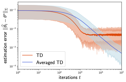
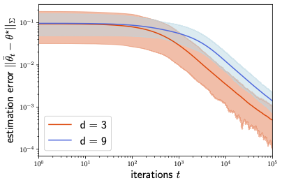
Figure 1: (a) Comparisons of the estimation error of TD and averaged TD when $d=3$. (b) Comparisons of the estimation error for averaged TD with $d=3$ and $d=9$. Two curves in the middle represent their average errors, while the shaded areas represent the $95\%$ confidence bands.

5.2 Off-policy evaluation: TDC learning

In order to demonstrate the efficiency of TDC for off-policy evaluation, we compare its performance with that of the off-policy TD learning on Baird’s counterexample (Baird,, 1995).

Baird’s counterexample.

We start by introducing Baird’s counterexample, which was constructed to illustrate the instability of TD learning in the off-policy regime. Consider an MDP $(\mathcal{S},\mathcal{A},\mathcal{P},r,\gamma)$, with the discount factor $\gamma=0.9$, state space $\mathcal{S}=[7]$, action space $\mathcal{A}=\{0,1\}$ and the reward function $r=0$ for all states and actions. The action $a=1$ transitions any initial state $s$ to $s^{\prime}=7$, while the action $a=0$ transitions any initial state $s$ to $s^{\prime}\in[6]$ with the same probability. The target policy $\pi$ selects $a=1$ at any given state $s$, while the behavior policy $\pi_{\mathsf{b}}$ takes $a=0$ with probability $\frac{6}{7}$ and $a=1$ with probability $\frac{1}{7}$. Formally, the MDP satisfies the equations (see also Figure 2 for an illustration)

$$\mathcal{P}(s^{\prime}|s,1)=\mathds{1}\{s^{\prime}=7\},\quad\forall s\in[7];\qquad\mathcal{P}(s^{\prime}|s,0)=\frac{1}{6}\mathds{1}\{1\leq s^{\prime}\leq 6\},\quad\forall s\in[7];$$

$$\pi(1|s)=1,\quad\forall s\in[7];$$

$$\pi_{\mathsf{b}}(0|s)=\frac{6}{7},\quad\forall s\in[7];\qquad\pi_{\mathsf{b}}(1|s)=\frac{1}{7},\quad\forall s\in[7].$$

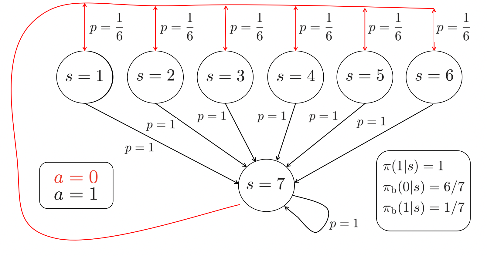
Figure 2: Baird’s counterexample. Taking action $a=1$ always leads to state $s=7$, while taking $a=0$ leads to one of the other six states with equal probability. The reward is set to be always zero.

In this example, it is easy to check that the stationary distribution corresponding to the behavior policy $\pi_{\mathsf{b}}$ is the uniform distribution among all states, and that the value function is $0$ for all states. We apply the following linear approximation of the value function: for $\bm{\theta}\in\mathbb{R}^{8}$,

$$\begin{cases}&V(i)=2\theta_{i}+\theta_{8},\quad\text{for}\quad 1\leq i\leq 6;\\ &V(7)=\theta_{7}+2\theta_{8}.\end{cases}$$ (40)

We remark that with this approximation, the feature space has a higher dimension ($d=8$) than the state space ($|\mathcal{S}|=7$). Consequently, the optimal estimator $\widetilde{\bm{\theta}}^{\star}$ is not unique, and instead can be any $\bm{\theta}\in\mathbb{R}^{8}$ such that the estimated value vector is $\bm{V}_{\bm{\theta}}=\bm{0}$. Technically, this issue can be circumvented by creating several identical states as state $s=7$; we omit this detail here for simplicity, since we use $\|\widehat{\bm{\theta}}_{t}-\widetilde{\bm{\theta}}^{\star}\|_{\widetilde{\bm{\Sigma}}}=\|\bm{V}_{\widehat{\bm{\theta}}_{t}}-\bm{V}^{\star}\|_{\bm{D}_{\mu_{\mathsf{b}}}}$ to evaluate the estimation error, and our experimental results would remain the same.

Experimental results.

We perform $100$ independent trials for both off-policy averaged TD learning (with stepsize $\eta=0.02$) and TDC (with stepsizes $\alpha=0.02,\beta=0.002$), starting at $\widehat{\bm{\theta}}_{0}=(1,1,1,1,1,1,10,1)^{\top}$, as suggested by Baird, (1995). In these experiments, we set $\alpha=\eta$ to ensure that the stepsize for $\bm{\theta}$-updates are the same between the two algorithms. Figure 3 demonstrates how the estimation error $\|\widehat{\bm{\theta}}_{t}-\widetilde{\bm{\theta}}^{\star}\|_{\widetilde{\bm{\Sigma}}}$ changes as two algorithms execute. As can be seen in this figure, TDC converges to an error of below $0.01$ after $T=10^{5}$ iterations while the off-policy averaged TD diverges to infinity.

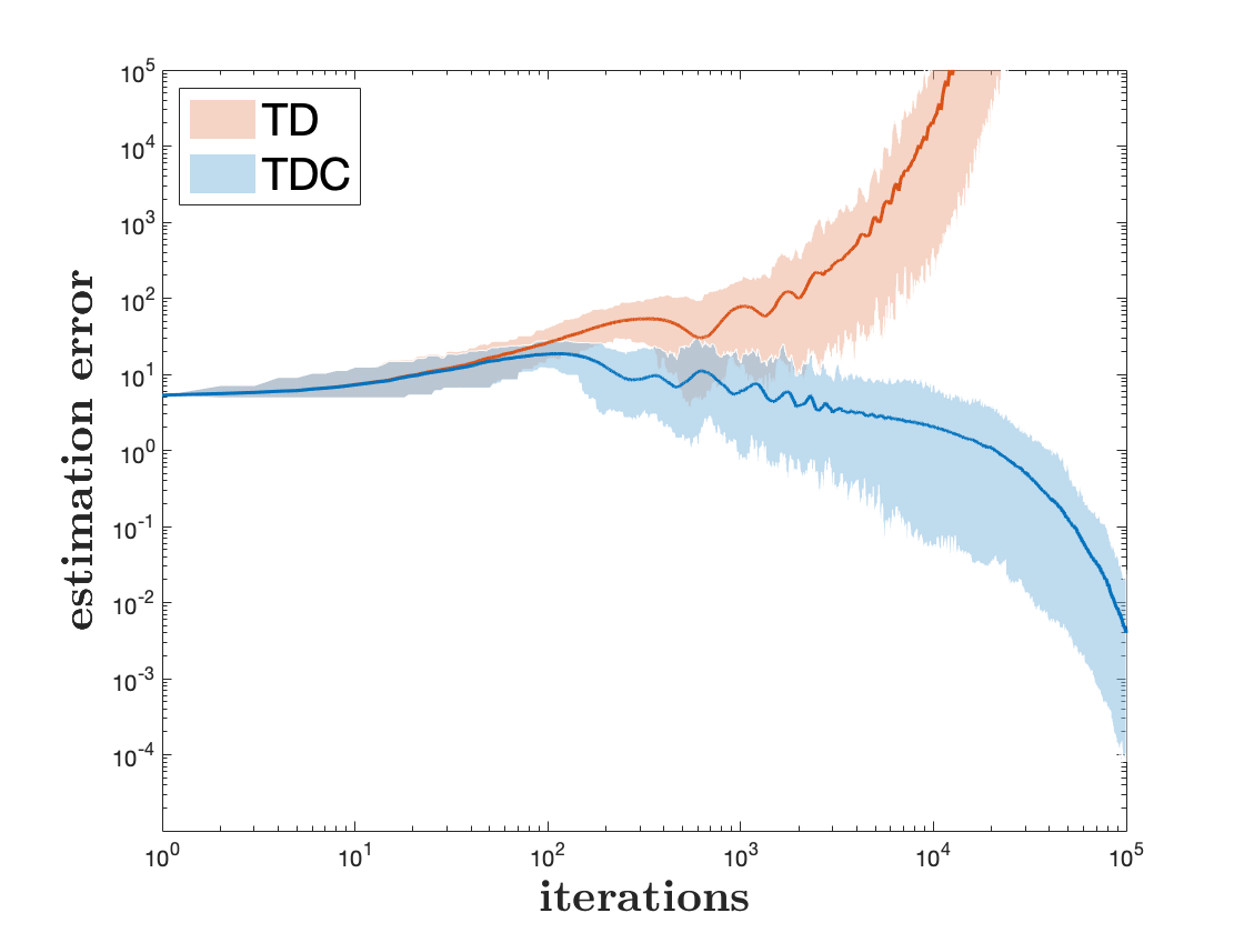
Figure 3: Performances of off-policy averaged TD (red, $\eta=0.02$) and TDC (blue, $\alpha=0.02$, $\beta=0.002$). Two curves in the middle represent their average errors, while the shaded areas correspond to $95\%$ confidence bands.

6 Proof of Theorem 1 (TD learning)

For the sake of convenience, let us introduce the following notation

$$\bm{\Delta}_{t}\coloneqq\bm{\bm{\theta}}_{t}-\bm{\theta}^{\star},\qquad\text{and}\qquad\overline{\bm{\Delta}}_{t}\coloneqq\overline{\bm{\theta}}_{t}-\bm{\theta}^{\star}.$$ (41)

Step 1: a recursive relation.

To understand the convergence behavior of $\overline{\bm{\Delta}}_{t}$, the idea is to first look at the following decomposition

$$\bm{\Delta}_{t+1} =\bm{\theta}_{t+1}-\bm{\theta}^{\star}=\bm{\theta}_{t}-\bm{\theta}^{\star}-\eta(\bm{A}_{t}\bm{\bm{\theta}}_{t}-\bm{b}_{t})$$

$$=\bm{\theta}_{t}-\bm{\theta}^{\star}-\eta\big{(}\bm{A}_{t}\bm{\bm{\theta}}_{t}-\bm{b}_{t}-(\bm{A}\bm{\theta}^{\star}-\bm{b})\big{)}$$

$$=\bm{\theta}_{t}-\bm{\theta}^{\star}-\eta\big{(}\bm{A}(\bm{\theta}_{t}-\bm{\theta}^{\star})+(\bm{A}_{t}-\bm{A})\bm{\theta}_{t}-(\bm{b}_{t}-\bm{b})\big{)}$$

$$=(\textbf{I}-\eta\bm{A})\bm{\Delta}_{t}-\eta\bm{\xi}_{t},$$

where we define

$$\bm{\xi}_{t}\coloneqq(\bm{A}_{t}-\bm{A})\bm{\theta}_{t}-(\bm{b}_{t}-\bm{b}).$$ (42)

Here, the second line invokes the update rule (14a) and the identity $\bm{A}\bm{\theta}^{\star}=\bm{b}$, whereas the third line is obtained by properly rearranging terms. Applying the above relation recursively, one arrives at

$$\bm{\Delta}_{t}=(\textbf{I}-\eta\bm{A})\bm{\Delta}_{t-1}-\eta\bm{\xi}_{t-1}=(\textbf{I}-\eta\bm{A})^{t}\bm{\Delta}_{0}-\eta\sum_{i=0}^{t-1}(\textbf{I}-\eta\bm{A})^{t-i-1}\bm{\xi}_{i}.$$ (43)

Step 2: a crude bound on $\|\bm{\Delta}_{t}\|_{\bm{\Sigma}}$.

We aim to establish, via an induction argument, that with probability at least $1-\delta$,

$$\|\bm{\Delta}_{t}\|_{\bm{\Sigma}}\leq 32\sqrt{\frac{\eta\kappa\log\frac{2dT}{\delta}}{1-\gamma}}(1+\|\bm{\theta}^{\star}\|_{\bm{\Sigma}})+2\sqrt{\kappa}\|\bm{\Delta}_{0}\|_{\bm{\Sigma}}\eqqcolon R_{0}$$ (44)

simultaneously over all $0\leq t\leq T$, as long as $0<\eta_{t}\leq\frac{c_{3}(1-\gamma)}{\kappa\log\frac{dT}{\delta}}$ for some sufficiently small constant $c_{3}>0$. As a side remark, this boundedness property saves us from enforcing additional projection steps as adopted in Bhandari et al., (2021).

To start with, note that the inequality (44) holds trivially for the base case with $t=0$, given that $\kappa\geq 1$. Next, suppose that the hypothesis (44) holds for $\bm{\Delta}_{0},\ldots,\bm{\Delta}_{t-1}$, and we intend to establish it for $\bm{\Delta}_{t}$ as well. Towards this end, invoking the decomposition (43) and the triangle inequality yields

$$\|\bm{\Delta}_{t}\|_{\bm{\Sigma}}\leq\big{\|}(\textbf{I}-\eta\bm{A})^{t}\bm{\Delta}_{0}\big{\|}_{\bm{\Sigma}}+\eta\,\Big{\|}\sum_{i=0}^{t-1}(\textbf{I}-\eta\bm{A})^{t-i-1}\bm{\xi}_{i}\Big{\|}_{\bm{\Sigma}}.$$ (45)

As for the first term of (45), it is seen that

$$\big{\|}(\textbf{I}-\eta\bm{A})^{t}\bm{\Delta}_{0}\big{\|}_{\bm{\Sigma}} =\big{\|}\bm{\Sigma}^{1/2}(\textbf{I}-\eta\bm{A})^{t}\bm{\Sigma}^{-1/2}\bm{\Sigma}^{1/2}\bm{\Delta}_{0}\big{\|}_{2}\leq\big{\|}\bm{\Sigma}^{1/2}\big{\|}\cdot\big{\|}\bm{\Sigma}^{-1/2}\big{\|}\cdot\big{\|}\textbf{I}-\eta\bm{A}\big{\|}^{t}\cdot\big{\|}\bm{\Sigma}^{1/2}\bm{\Delta}_{0}\big{\|}_{2}$$

$$\leq\sqrt{\kappa}\left(1-\frac{1}{2}\eta(1-\gamma)\lambda_{\mathsf{min}}(\bm{\Sigma})\right)^{t}\|\bm{\Delta}_{0}\|_{\bm{\Sigma}}\leq\sqrt{\kappa}\|\bm{\Delta}_{0}\|_{\bm{\Sigma}},$$ (46)

where the last inequality arises from the definition of $\kappa$ and the property (89g) (with the restriction that $\eta\leq(1-\gamma)/(4\|\bm{\Sigma}\|)$). When it comes to the second term of (45), the following lemma comes in handy.

Lemma 1.

Fix any quantity $R>0$ and, for each $0\leq i\leq T-1$, define the auxiliary random vector

$$\bm{\widetilde{\xi}}_{i}\coloneqq\bm{\xi}_{i}\,\mathds{1}\{\mathcal{H}_{i}\},\qquad\text{where}\quad\mathcal{H}_{i}\coloneqq\Big{\{}\|\bm{\Delta}_{i}\|_{\bm{\Sigma}}\leq R\Big{\}}.$$ (47)

Then, with probability at least $1-\delta/T$, simultaneously over the indices $(l,u,t)$ such that $0\leq l\leq u\leq t-1<T$ it holds that

$$\Big{\|}\sum_{i=l}^{u}(\textbf{I}-\eta\bm{A})^{t-i-1}\bm{\widetilde{\xi}}_{i}\Big{\|}_{\bm{\Sigma}}\leq 16\Big{(}1-\frac{1}{2}\eta(1-\gamma)\lambda_{\min}(\bm{\Sigma})\Big{)}^{t-u-1}(\|\bm{\theta}^{\star}\|_{\bm{\Sigma}}+R+1)\sqrt{\frac{\kappa\log\frac{2dT}{\delta}}{\eta(1-\gamma)}},$$

provided that $0<\eta_{t}\leq\frac{1-\gamma}{\kappa\log\frac{2dT}{\delta}}$.

Proof.

See Section C.1. ∎

Under the induction hypothesis that $\|\bm{\Delta}_{i}\|_{\bm{\Sigma}}\leq R_{0}$ for $0\leq i\leq t-1$, we can invoke Lemma 1 (with $R=R_{0},l=0$ and $u=t-1$) to show that

$$\Big{\|}\sum_{i=0}^{t-1}(\textbf{I}-\eta\bm{A})^{t-i-1}\bm{{\xi}}_{i}\Big{\|}_{\bm{\Sigma}} =\Big{\|}\sum_{i=0}^{t-1}(\textbf{I}-\eta\bm{A})^{t-i-1}\bm{{\xi}}_{i}\mathds{1}\{\|\bm{\Delta}_{i}\|_{\bm{\Sigma}}\leq R_{0}\}\Big{\|}_{\bm{\Sigma}}$$

$$\leq 16(\|\bm{\theta}^{\star}\|_{\bm{\Sigma}}+R_{0}+1)\sqrt{\frac{\kappa\log\frac{2dT}{\delta}}{\eta(1-\gamma)}}$$ (48)

holds with probability at least $1-\delta/T$, provided that $0<\eta\leq\frac{1-\gamma}{\kappa\log\frac{dT}{\delta}}$. Combining (45), (46) and (48) together and recalling the definition (44) of $R_{0}$, we can easily verify that

$$\|\bm{\Delta}_{t}\|_{\bm{\Sigma}}\leq\sqrt{\kappa}\|\bm{\Delta}_{0}\|_{\bm{\Sigma}}+16(\|\bm{\theta}^{\star}\|_{\bm{\Sigma}}+R_{0}+1)\sqrt{\frac{\eta\kappa\log\frac{2dT}{\delta}}{1-\gamma}}\leq R_{0},$$ (49)

with the proviso that $32\sqrt{\frac{\eta\kappa\log(2dT/\delta)}{1-\gamma}}\leq 1$. The induction argument coupled with the union bound then establishes the claim (44).

Step 3: a refined bound on $\|\bm{\Delta}_{t}\|_{\bm{\Sigma}}$.

It turns out that the upper bound (44) is somewhat loose due to the complete ignorance of the contraction effect of $\textbf{I}-\eta\bm{A}$; see (46). In what follows, we develop a strengthened bound. Define

$$t_{\mathsf{seg}}:=\frac{c_{1}\log\max\{4\sqrt{\kappa},\frac{16\kappa\|\bm{\Delta}_{0}\|_{\bm{\Sigma}}}{\|\bm{\theta}^{\star}\|_{\bm{\Sigma}}+1},\|\bm{\Delta}_{0}\|_{\bm{\Sigma}}\sqrt{\frac{1-\gamma}{\eta\kappa\log\frac{2dT}{\delta}}}\}}{\eta(1-\gamma)\lambda_{\mathsf{min}}(\bm{\Sigma})}$$ (50)

for some sufficiently large constant $c_{1}>0$. For any integer $k\geq 1$, we aim to establish that

$$\|\bm{\Delta}_{t}\|_{\bm{\Sigma}}\leq 32\sqrt{\frac{\eta\kappa\log\frac{2dT}{\delta}}{1-\gamma}}\Big{(}\|\bm{\theta}^{\star}\|_{\bm{\Sigma}}+\frac{\sqrt{\kappa}\|\bm{\Delta}_{0}\|_{\bm{\Sigma}}}{2^{k-1}}+\frac{3}{2}\Big{)}\eqqcolon R_{k}$$ (51)

for any $t$ obeying $kt_{\mathsf{seg}}\leq t\leq T$, provided that $0<\eta\leq\frac{c_{3}(1-\gamma)}{\kappa\log\frac{dT}{\delta}}$ for some small enough constant $c_{3}>0$.

Because of relation (45), we claim that it suffices to prove that

$$\Big{\|}\sum_{i=0}^{t-1}(\textbf{I}-\eta\bm{A})^{t-i-1}\bm{\xi}_{i}\Big{\|}_{\bm{\Sigma}}\leq 32\Big{(}\|\bm{\theta}^{\star}\|_{\bm{\Sigma}}+\frac{2\sqrt{\kappa}\|\bm{\Delta}_{0}\|_{\bm{\Sigma}}}{2^{k}}+1\Big{)}\sqrt{\frac{\kappa\log\frac{2dT}{\delta}}{\eta(1-\gamma)}},\qquad kt_{\mathsf{seg}}\leq t\leq T.$$ (52)

To see this: note that the first term on the right-hand side of (45) has already been bounded in (46), which combined with the definition (50) of $t_{\mathsf{seg}}$ indicates that

$$\big{\|}\bm{\Sigma}^{1/2}(\textbf{I}-\eta\bm{A})^{t}\bm{\Delta}_{0}\big{\|}_{2}\leq\sqrt{\kappa}\left(1-\frac{1}{2}\eta(1-\gamma)\lambda_{\mathsf{min}}(\bm{\Sigma})\right)^{t_{\mathsf{seg}}}\|\bm{\Delta}_{0}\|_{\bm{\Sigma}}\leq\sqrt{\frac{\eta\kappa\log\frac{2dT}{\delta}}{1-\gamma}}$$ (53)

for any $t\geq t_{\mathsf{seg}}$. Clearly, combining (52) with (45) and (53) shall immediately lead to the claim (51). The remainder of this step is thus devoted to demonstrating (52) inductively.

The base case (i.e. $k=1$) follows immediately from our bounds (44) and (48) in Step 2, given that $\sqrt{\frac{\eta\kappa\log\frac{2dT}{\delta}}{1-\gamma}}$ is sufficiently small. Suppose now that the claim (52) holds for a given integer $k\geq 1$ and any $t$ obeying $kt_{\mathsf{seg}}\leq t\leq T$, and we intend to show that (52) continues to hold for $k+1$ and any $t$ obeying $(k+1)t_{\mathsf{seg}}\leq t\leq T$. Towards this, we first single out the following straightforward decomposition

$$\Big{\|}\sum_{i=0}^{t-1}(\textbf{I}-\eta\bm{A})^{t-i-1}\bm{\xi}_{i}\Big{\|}_{\bm{\Sigma}} \leq\Big{\|}\sum_{i=t-t_{\mathsf{seg}}+1}^{t-1}(\textbf{I}-\eta\bm{A})^{t-i-1}\bm{\xi}_{i}\Big{\|}_{\bm{\Sigma}}+\Big{\|}\sum_{i=0}^{t-t_{\mathsf{seg}}}(\textbf{I}-\eta\bm{A})^{t-i-1}\bm{\xi}_{i}\Big{\|}_{\bm{\Sigma}},$$

which allows us to upper bound the two terms on the right-hand side above seperately.

• Under the induction hypothesis that $\|\bm{\Delta}_{i}\|_{\bm{\Sigma}}\leq R_{k}$ for all $i$ obeying $kt_{\mathsf{seg}}\leq i\leq T$, one can invoke Lemma 1 with $R=R_{k},l=t-t_{\mathsf{seg}}+1$ and $u=t-1$ to see that

  $$\Big{\|}\sum_{i=t-t_{\mathsf{seg}}+1}^{t-1}(\textbf{I}-\eta\bm{A})^{t-i-1}\bm{\xi}_{i}\Big{\|}_{\bm{\Sigma}} =\Big{\|}\sum_{i=t-t_{\mathsf{seg}}+1}^{t-1}(\textbf{I}-\eta\bm{A})^{t-i-1}\bm{\xi}_{i}\mathds{1}\{\|\bm{\Delta}_{i}\|_{\bm{\Sigma}}\leq R_{k}\}\Big{\|}_{\bm{\Sigma}}$$

  $$\leq 16\big{(}\|\bm{\theta}^{\star}\|_{\bm{\Sigma}}+R_{k}+1\big{)}\sqrt{\frac{\kappa\log\frac{2dT}{\delta}}{\eta(1-\gamma)}}$$

  $$\leq 24\Big{(}\|\bm{\theta}^{\star}\|_{\bm{\Sigma}}+\frac{2\sqrt{\kappa}\|\bm{\Delta}_{0}\|_{\bm{\Sigma}}}{2^{k+1}}+1\Big{)}\sqrt{\frac{\kappa\log\frac{2dT}{\delta}}{\eta(1-\gamma)}},$$

  where the last line uses the definition (51) of $R_{k}$ and holds as long as $\frac{\eta\kappa\log\frac{2dT}{\delta}}{1-\gamma}$ is sufficiently small.

• In addition, we make the observation that: for any $t\geq t_{\mathsf{seg}}$,

  $$\Big{\|}\sum_{i=0}^{t-t_{\mathsf{seg}}}(\textbf{I}-\eta\bm{A})^{t-i-1}\bm{\xi}_{i}\Big{\|}_{\bm{\Sigma}} =\Big{\|}\sum_{i=0}^{t-t_{\mathsf{seg}}}(\textbf{I}-\eta\bm{A})^{t-i-1}\bm{\xi}_{i}\mathds{1}\{\|\bm{\Delta}_{i}\|_{\bm{\Sigma}}\leq R_{0}\}\Big{\|}_{\bm{\Sigma}}$$

  $$\leq 16(1-\frac{1}{2}\eta(1-\gamma)\lambda_{\min}(\bm{\Sigma}))^{t_{\mathsf{seg}}-1}(\|\bm{\theta}^{\star}\|_{\bm{\Sigma}}+R_{0}+1)\sqrt{\frac{\kappa\log\frac{2dT}{\delta}}{\eta(1-\gamma)}}$$

  $$\leq 8\big{(}\|\bm{\theta}^{\star}\|_{\bm{\Sigma}}+1\big{)}\sqrt{\frac{\kappa\log\frac{2dT}{\delta}}{\eta(1-\gamma)}}.$$

  Here, the first equality uses the crude bound $\|\bm{\Delta}_{i}\|_{\bm{\Sigma}}\leq R_{0}$ for all $i$ (see (44)), the second to last inequality utilizes Lemma 1 with $R=R_{0},l=0$ and $u=t-t_{\mathsf{seg}}$, whereas the last inequality relies on the definition (44) of $R_{0}$ and invokes the fact that $\sqrt{\kappa}\left(1-\frac{1}{2}\eta(1-\gamma)\lambda_{\mathsf{min}}(\bm{\Sigma})\right)^{t_{\mathsf{seg}}-1}\leq\min\big{\{}\frac{1}{4},\frac{1}{4\sqrt{\kappa}\|\bm{\Delta}_{0}\|_{\bm{\Sigma}}}\big{\}}$ with our choice (50) of $t_{\mathsf{seg}}$.

Combine the previous two bounds to reach

$$\Big{\|}\sum_{i=0}^{t-1}(\textbf{I}-\eta\bm{A})^{t-i-1}\bm{\xi}_{i}\Big{\|}_{\bm{\Sigma}} \leq 24\Big{(}\|\bm{\theta}^{\star}\|_{\bm{\Sigma}}+\frac{2\sqrt{\kappa}\|\bm{\Delta}_{0}\|_{\bm{\Sigma}}}{2^{k+1}}+1\Big{)}\sqrt{\frac{\kappa\log\frac{2dT}{\delta}}{\eta(1-\gamma)}}+8\big{(}\|\bm{\theta}^{\star}\|_{\bm{\Sigma}}+1\big{)}\sqrt{\frac{\kappa\log\frac{2dT}{\delta}}{\eta(1-\gamma)}}$$

$$\leq 32\Big{(}\|\bm{\theta}^{\star}\|_{\bm{\Sigma}}+\frac{2\sqrt{\kappa}\|\bm{\Delta}_{0}\|_{\bm{\Sigma}}}{2^{k}}+1\Big{)}\sqrt{\frac{\kappa\log\frac{2dT}{\delta}}{\eta(1-\gamma)}}.$$

This finishes the induction step and in turn establishes (52) (and hence (51)).

As a straightforward consequence, the bounds (44) and (51) imply that

$$\|\bm{\Delta}_{t}\|_{\bm{\Sigma}}\leq\begin{cases}R_{0},\qquad&0\leq t<t_{\mathsf{seg}}^{\prime},\\ 32\sqrt{\frac{\eta\kappa\log\frac{2dT}{\delta}}{1-\gamma}}(\|\bm{\theta}^{\star}\|_{\bm{\Sigma}}+2),\qquad&t_{\mathsf{seg}}^{\prime}\leq t<T,\end{cases}$$ (54)

where

$$t_{\mathsf{seg}}^{\prime}\coloneqq c_{2}t_{\mathsf{seg}}\log\big{(}\kappa(\|\bm{\Delta}_{0}\|_{2}+1)\big{)}$$ (55)

for some large enough constant $c_{2}>0$. To see this, note that for any $t\geq t_{\mathsf{seg}}^{\prime}$, it is guaranteed that the second term on the right-hand side of (51) obeys $\frac{4\sqrt{\kappa}\|\bm{\Delta}_{0}\|_{\bm{\Sigma}}}{2^{\lfloor t/t_{\mathsf{seg}}\rfloor}}\leq 2$, thus confirming the second case in (54).

Step 4: controlling $\|\overline{\bm{\Delta}}_{T}\|_{\bm{\Sigma}}$.

Now we are positioned to control $\overline{\bm{\Delta}}_{T}$. The key is to write $\overline{\bm{\Delta}}_{T}$ as a linear combination of $\{\bm{\xi}_{i}\}_{0\leq i\leq T-1}$ as follows, which is a direct consequence of the relation (43):

$$\overline{\bm{\Delta}}_{T} =\frac{1}{T}\sum_{j=1}^{T}\bm{\Delta}_{j}=\frac{1}{T}\sum_{j=1}^{T}(\textbf{I}-\eta\bm{A})^{j}\bm{\Delta}_{0}-\frac{1}{T}\sum_{j=1}^{T}\eta\sum_{i=0}^{j-1}(\textbf{I}-\eta\bm{A})^{j-i-1}\bm{\xi}_{i}$$

$$=\frac{1}{T}\sum_{j=1}^{T}(\textbf{I}-\eta\bm{A})^{j}\bm{\Delta}_{0}-\frac{1}{T}\sum_{i=0}^{T-1}\eta\sum_{j=i+1}^{T}(\textbf{I}-\eta\bm{A})^{j-i-1}\bm{\xi}_{i}$$

$$=\frac{1}{T\eta}\bm{A}_{0}^{(T+1)}\bm{\Delta}_{0}-\frac{1}{T}\bm{\Delta}_{0}-\frac{1}{T}\sum_{i=0}^{T-1}\bm{A}_{i}^{(T)}\bm{\xi}_{i},$$ (56)

where the middle line follows from swapping the summation over $i$ and $j$, and in the last line we define

$$\bm{A}_{i}^{(t)}\coloneqq\eta\sum_{j=i+1}^{t}(\textbf{I}-\eta\bm{A})^{j-i-1}=\bm{A}^{-1}\big{(}\textbf{I}-(\textbf{I}-\eta\bm{A})^{t-i}\big{)}.$$ (57)

We claim that the following two inequalities hold, the first deterministically and the second with probability of at least $1-\delta$ (with their proofs deferred to Section C.2)

$$\big{\|}\bm{A}_{0}^{(T+1)}\bm{\Delta}_{0}\big{\|}_{\bm{\Sigma}} \leq\frac{2\|\bm{\Sigma}^{-1}\|}{1-\gamma}\big{\|}\bm{\Delta}_{0}\|_{\bm{\Sigma}};$$ (58a)

$$\Big{\|}\sum_{i=0}^{T-1}\bm{A}_{i}^{(T)}\bm{\xi}_{i}\Big{\|}_{\bm{\Sigma}} \lesssim\left\{\sqrt{\frac{\max_{s}\bm{\phi}(s)^{\top}\bm{\Sigma}^{-1}\bm{\phi}(s)\log\frac{2d}{\delta}}{T(1-\gamma)^{2}}}+\frac{\big{\|}\bm{\Sigma}^{-1}\big{\|}}{T}\sqrt{\frac{\kappa\log\frac{2dT}{\delta}}{\eta(1-\gamma)^{3}}}\right\}\big{(}\|\bm{\theta}^{\star}\|_{\bm{\Sigma}}+1\big{)}.$$ (58b)

Putting the above two inequalities together with (56), we arrive at

$$\|\overline{\bm{\Delta}}_{T}\|_{\bm{\Sigma}}\leq\Big{\|}\frac{1}{T\eta}\bm{A}_{0}^{(T+1)}\bm{\Delta}_{0}\Big{\|}_{\bm{\Sigma}}+\Big{\|}\frac{1}{T}\bm{\Delta}_{0}\Big{\|}_{\bm{\Sigma}}+\Big{\|}\frac{1}{T}\sum_{i=0}^{T-1}\bm{A}_{i}^{(T)}\bm{\xi}_{i}\Big{\|}_{\bm{\Sigma}}$$

$$\leavevmode\nobreak\ \leavevmode\nobreak\ \lesssim\frac{1}{\eta T}\frac{\big{\|}\bm{\Sigma}^{-1}\big{\|}}{1-\gamma}\big{\|}\bm{\Delta}_{0}\|_{\bm{\Sigma}}+\frac{1}{T}\|\bm{\Delta}_{0}\|_{\bm{\Sigma}}+\left\{\sqrt{\frac{\max_{s}\bm{\phi}(s)^{\top}\bm{\Sigma}^{-1}\bm{\phi}(s)\log\frac{2d}{\delta}}{T(1-\gamma)^{2}}}+\frac{\big{\|}\bm{\Sigma}^{-1}\big{\|}}{T}\sqrt{\frac{\kappa\log\frac{2dT}{\delta}}{\eta(1-\gamma)^{3}}}\right\}\big{(}\|\bm{\theta}^{\star}\|_{\bm{\Sigma}}+1\big{)}$$

$$\leavevmode\nobreak\ \leavevmode\nobreak\ \asymp\frac{1}{\eta T}\frac{\big{\|}\bm{\Sigma}^{-1}\big{\|}}{1-\gamma}\big{\|}\bm{\Delta}_{0}\|_{\bm{\Sigma}}+\left\{\sqrt{\frac{\max_{s}\bm{\phi}(s)^{\top}\bm{\Sigma}^{-1}\bm{\phi}(s)\log\frac{2d}{\delta}}{T(1-\gamma)^{2}}}+\frac{\big{\|}\bm{\Sigma}^{-1}\big{\|}}{T}\sqrt{\frac{\kappa\log\frac{2dT}{\delta}}{\eta(1-\gamma)^{3}}}\right\}\big{(}\|\bm{\theta}^{\star}\|_{\bm{\Sigma}}+1\big{)},$$

where the last line follows since $\|\bm{\Sigma}^{-1}\|\geq 1$ (see (89h)) and $\eta<1$. This finishes the proof of Theorem 1.

7 Proof of Theorem 3 (TDC learning)

Firstly, let us analyze the population dynamics of TDC. It turns out that the convergence of this dynamics can be described via a contractive linear mapping. Given this nice property of population TDC, we shall decompose the empirical TDC into two parts: the first part can be controlled via the aforementioned population dynamics, and the rest is treated as a stochastic component, which is controlled via matrix martingale concentration.

7.1 Population analysis

First recall that the population parameters are defined as

$$\widetilde{\bm{A}} \coloneqq\mathbb{E}_{\mu_{\mathsf{b}},\pi_{\mathsf{b}},\mathcal{P}}[\widetilde{\bm{A}}_{t}]=\mathbb{E}_{\mu_{\mathsf{b}},\pi_{\mathsf{b}},\mathcal{P}}[\rho_{t}\bm{\phi}(s_{t})\left(\bm{\phi}(s_{t})-\gamma\bm{\phi}(s_{t}^{\prime})\right)^{\top}];$$

$$\widetilde{\bm{b}} \coloneqq\mathbb{E}_{\mu_{\mathsf{b}},\pi_{\mathsf{b}}}[\widetilde{\bm{b}}_{t}]=\mathbb{E}_{\mu_{\mathsf{b}},\pi_{\mathsf{b}}}[\rho_{t}\bm{\phi}(s_{t})r_{t}];$$

$$\bm{\Pi} \coloneqq\mathbb{E}_{\mu_{\mathsf{b}},\pi_{\mathsf{b}},\mathcal{P}}[\bm{\Pi}_{t}]=\mathbb{E}_{\mu_{\mathsf{b}},\pi_{\mathsf{b}},\mathcal{P}}[\rho_{t}\bm{\phi}(s_{t})\bm{\phi}(s_{t}^{\prime})^{\top}];$$

$$\widetilde{\bm{\Sigma}} \coloneqq\mathbb{E}_{\mu_{\mathsf{b}}}[\bm{\Sigma}_{t}]=\mathbb{E}_{\mu_{\mathsf{b}}}[\bm{\phi}(s_{t})\bm{\phi}(s_{t})^{\top}].$$

Corresponding to the empirical version of TDC as given in (31), we can define its population analogue of TDC as

$$\breve{\bm{\theta}}_{t+1} =\breve{\bm{\theta}}_{t}-\alpha(\widetilde{\bm{A}}\breve{\bm{\theta}}_{t}-\widetilde{\bm{b}}+\gamma\bm{\Pi}^{\top}\breve{\bm{w}}_{t}),$$

$$\breve{\bm{w}}_{t+1} =\breve{\bm{w}}_{t}-\beta(\widetilde{\bm{A}}\breve{\bm{\theta}}_{t}-\widetilde{\bm{b}}+\widetilde{\bm{\Sigma}}\breve{\bm{w}}_{t}),$$ (59)

where sampled parameters are replaced by their corresponding expectations. In this section, we analyze the population dynamics of TDC as given above; in order to control the finite-sample dynamics, we bound the difference of these two in the section to follow.

Since $\bm{\phi}(s_{t})$ is independent of the transition, the expectation of $\widetilde{\bm{\Sigma}}_{t}$ is independent of which policy is being adopted. Hence, $\widetilde{\bm{\Sigma}}$ can also be presented as

$$\widetilde{\bm{\Sigma}} =\sum_{s_{t}\in\mathcal{S}}\mu_{\mathsf{b}}(s_{t})\bm{\phi}(s_{t})\bm{\phi}(s_{t})^{\top}$$

$$=\sum_{s_{t}\in\mathcal{S}}\mu_{\mathsf{b}}(s_{t})\left(\sum_{a_{t}\in\mathcal{A}}\pi(a_{t}|s_{t})\right)\bm{\phi}(s_{t})\bm{\phi}(s_{t})^{\top}$$

$$=\sum_{s_{t}\in\mathcal{S}}\sum_{a_{t}\in\mathcal{A}}\mu_{\mathsf{b}}(s_{t})\pi_{\mathsf{b}}(a_{t}|s_{t})\left(\frac{\pi(a_{t}|s_{t})}{\pi_{\mathsf{b}}(a_{t}|s_{t})}\right)\bm{\phi}(s_{t})\bm{\phi}(s_{t})^{\top}=\mathbb{E}_{\mu_{\mathsf{b}},\pi_{\mathsf{b}}}[\rho_{t}\bm{\phi}(s_{t})\bm{\phi}(s_{t})^{\top}].$$ (60)

In view of this relation, $\widetilde{\bm{A}}$ admits another characterization, namely

$$\widetilde{\bm{A}}=\widetilde{\bm{\Sigma}}-\gamma\bm{\Pi}.$$ (61)

Consequently, the fixed point $(\breve{\bm{\theta}}^{\star},\bm{w}^{\star})$ of the population dynamics obeys

$$\begin{cases}\widetilde{\bm{A}}\breve{\bm{\theta}}^{\star}-\widetilde{\bm{b}}+\gamma\bm{\Pi}^{\top}\bm{w}^{\star}=\bm{0},\\ \widetilde{\bm{A}}\breve{\bm{\theta}}^{\star}-\widetilde{\bm{b}}+\widetilde{\bm{\Sigma}}\bm{w}^{\star}=\bm{0}.\end{cases}$$

As long as $\widetilde{\bm{A}}$ is invertible, this set of conditions is equivalent to

$$\widetilde{\bm{A}}\breve{\bm{\theta}}^{\star}=\widetilde{\bm{b}},\qquad\text{and}\qquad\bm{w}^{\star}=\bm{0}.$$

In order to study the population dynamics, it is useful to consider two auxiliary parameters

$$\breve{\bm{\Delta}}_{t} \coloneqq\breve{\bm{\theta}}_{t}-\breve{\bm{\theta}}^{\star},$$

$$\breve{\bm{z}}_{t} \coloneqq\breve{\bm{w}}_{t}+\widetilde{\bm{\Sigma}}^{-1}\widetilde{\bm{A}}\breve{\bm{\Delta}}_{t};$$

here $\breve{\bm{\Delta}}_{t}$ tracks the convergence of $\breve{\bm{\theta}}_{t}$ to $\breve{\bm{\theta}}^{\star}$, and $\breve{\bm{z}}_{t}$ tracks the size of the residual $\widetilde{\bm{A}}\breve{\bm{\theta}}_{t}-\widetilde{\bm{b}}+\widetilde{\bm{\Sigma}}\breve{\bm{w}}_{t}$. With these two parameters in place, the population dynamics satisfy

$$\left[\begin{array}[]{c}\breve{\bm{\Delta}}_{t}\\ \breve{\bm{z}}_{t}\end{array}\right]=\left[\begin{array}[]{cc}\bm{I}-\alpha\widetilde{\bm{A}}^{\top}\widetilde{\bm{\Sigma}}^{-1}\widetilde{\bm{A}}&-\alpha\gamma\bm{\Pi}^{\top}\\ -\alpha(\bm{I}-\gamma\bm{\Sigma}^{-1}\bm{\Pi})\widetilde{\bm{A}}^{\top}\widetilde{\bm{\Sigma}}^{-1}\widetilde{\bm{A}}&\bm{I}-\beta\widetilde{\bm{\Sigma}}-\alpha\gamma(\bm{I}-\gamma\widetilde{\bm{\Sigma}}^{-1}\bm{\Pi})\bm{\Pi}^{\top}\end{array}\right]\left[\begin{array}[]{c}\breve{\bm{\Delta}}_{t-1}\\ \breve{\bm{z}}_{t-1}\end{array}\right].$$ (68)

To analyze this optimization dynamics, for every positive constant $\varkappa\in(0,1)$, consider

$$\breve{\bm{x}}_{t}\coloneqq\left[\begin{array}[]{c}\breve{\bm{\Delta}}_{t}\\ \varkappa\breve{\bm{z}}_{t}\end{array}\right]$$

then $\breve{\bm{x}}_{t}$ yields

$$\breve{\bm{x}}_{t}=\underbrace{\left[\begin{array}[]{cc}\bm{I}-\alpha\widetilde{\bm{A}}^{\top}\widetilde{\bm{\Sigma}}^{-1}\widetilde{\bm{A}}&-\frac{1}{\varkappa}\alpha\gamma\bm{\Pi}^{\top}\\ -\varkappa\alpha(\bm{I}-\gamma\bm{\Sigma}^{-1}\bm{\Pi})\widetilde{\bm{A}}^{\top}\widetilde{\bm{\Sigma}}^{-1}\widetilde{\bm{A}}&\bm{I}-\beta\widetilde{\bm{\Sigma}}-\alpha\gamma(\bm{I}-\gamma\widetilde{\bm{\Sigma}}^{-1}\bm{\Pi})\bm{\Pi}^{\top}\end{array}\right]}_{\eqqcolon\bm{\Psi}}\breve{\bm{x}}_{t-1}.$$ (71)

It is known that how fast $\breve{\bm{x}}_{t}$ converges to $\bm{0}$ is determined by the spectral norm of $\bm{\Psi}$, which is characterized in the lemma below.

Lemma 2.

Suppose that

$$\lambda_{1}=\lambda_{\min}(\widetilde{\bm{A}}^{\top}\widetilde{\bm{\Sigma}}^{-1}\widetilde{\bm{A}}),\quad\lambda_{2}=\lambda_{\min}(\widetilde{\bm{\Sigma}}),\quad\lambda_{\Sigma}=\|\widetilde{\bm{\Sigma}}^{-1}\|=1/\lambda_{2}.$$

Then as long as the following conditions hold:

$$\beta \gtrsim\lambda_{\Sigma}\rho_{\max}\alpha,$$ (72a)

$$\varkappa\beta \gtrsim\alpha,$$ (72b)

$$\alpha\gamma(\rho_{\max}+\gamma\lambda_{\Sigma}\rho_{\max}^{2}) \ll\beta\lambda_{w},$$ (72c)

$$\frac{\alpha\gamma\rho_{\max}}{\varkappa}+\varkappa\alpha(1+\gamma\lambda_{\Sigma}\rho_{\max})\lambda_{\Sigma}(2\rho_{\max})^{2} \ll\sqrt{\alpha\lambda_{1}\beta\lambda_{w}}$$ (72d)

it holds true that

$$\|\bm{\Psi}\|\leq 1-\frac{1}{2}\alpha\lambda_{1}.$$

Therefore, the mapping $\bm{\Psi}$ is contractive, thus ensuring the linear convergence of $\bm{x}_{t}$, with the proviso that $\alpha\lambda_{1}<2.$

7.2 Finite-sample analysis

Armed with the population analysis, the proof for Theorem 3 is completed if we can make a connection of the finite-sample performances to that of the population ones.

Step 1: a recursive relation.

Firstly, we define two noise variables

$$\bm{\nu}_{t} \coloneqq(\widetilde{\bm{A}}_{t}-\widetilde{\bm{A}})\widetilde{\bm{\theta}}_{t}-(\widetilde{\bm{b}}_{t}-\widetilde{\bm{b}})+\gamma(\bm{\Pi}_{t}-\bm{\Pi})^{\top}\bm{w}_{t},$$

$$\bm{\eta}_{t} \coloneqq(\widetilde{\bm{A}}_{t}-\widetilde{\bm{A}})\widetilde{\bm{\theta}}_{t}-(\widetilde{\bm{b}}_{t}-\widetilde{\bm{b}})+(\widetilde{\bm{\Sigma}}_{t}-\widetilde{\bm{\Sigma}})\bm{w}_{t}.$$

As a result, TDC can be rewritten as

$$\widetilde{\bm{\theta}}_{t+1} =\widetilde{\bm{\theta}}_{t}-\alpha(\widetilde{\bm{A}}\widetilde{\bm{\theta}}_{t}-\widetilde{\bm{b}}+\gamma\bm{\Pi}^{\top}\bm{w}_{t})-\alpha\bm{\nu}_{t};$$

$$\bm{w}_{t+1} =\bm{w}_{t}-\beta(\widetilde{\bm{A}}\widetilde{\bm{\theta}}_{t}-\widetilde{\bm{b}}+\widetilde{\bm{\Sigma}}\bm{w}_{t})-\beta\bm{\eta}_{t}.$$

Using the same notations as in Section 7.1, we observe that the following iteration holds true for finite-sample TDC:

$$\bm{x}_{t+1}=\bm{\Psi}\bm{x}_{t}-\bm{\zeta}_{t},$$

in which

$$\bm{\zeta}_{t}=\left[\begin{array}[]{c}\alpha\bm{\nu}_{t}\\ \varkappa(\alpha(1-\gamma\widetilde{\bm{\Sigma}}^{-1}\bm{\Pi})\bm{\nu}_{t}+\beta\bm{\eta}_{t})\end{array}\right].$$ (75)

Hence,

$$\bm{x}_{t}=\bm{\Psi}^{t}\bm{x}_{0}-\sum_{i=0}^{t-1}\bm{\Psi}^{t-i-1}\bm{\zeta}_{i},$$ (76)

where $\bm{x}_{0}=[\bm{\Delta}_{0}^{\top},\varkappa\bm{z}_{0}^{\top}]^{\top}$. Since the norm of $\bm{\Psi}$ has been bounded by Lemma 2, bounding the norm of $\bm{x}_{t}$ boils down to bounding the second term of (76). In the following, with a slight abuse of notation, for any $\bm{x}=(\bm{x}_{1},\bm{x}_{2})\in\mathbb{R}^{2d}$ with $\bm{x}_{1},\bm{x}_{2}\in\mathbb{R}^{d}$, we will define $\|\bm{x}\|_{\widetilde{\bm{\Sigma}}}^{2}$ as

$$\|\bm{x}\|_{\widetilde{\bm{\Sigma}}}^{2}=\|\bm{x}_{1}\|_{\widetilde{\bm{\Sigma}}}^{2}+\|\bm{x}_{2}\|_{\widetilde{\bm{\Sigma}}}^{2}.$$

with this definition, it is easy to see that

$$\|\bm{x}_{t}\|_{\widetilde{\bm{\Sigma}}}^{2}=\|\tilde{\bm{\Delta}}_{t}\|_{\widetilde{\bm{\Sigma}}}^{2}+\varkappa^{2}\|\bm{w}_{t}+\widetilde{\bm{\Sigma}}^{-1}\widetilde{\bm{A}}\widetilde{\bm{\Delta}}_{t}\|_{\widetilde{\bm{\Sigma}}}^{2}.$$

Hence, the norms of $\widetilde{\bm{\Delta}}_{t}$, $\bm{w}_{t}$ and $\bm{x}_{t}$ can be related by the inequalities

$$\begin{cases}&\|\widetilde{\bm{\Delta}}_{t}\|_{\widetilde{\bm{\Sigma}}}\leq\|\bm{x}_{t}\|_{\widetilde{\bm{\Sigma}}};\\ &\|\bm{w}_{t}\|_{\widetilde{\bm{\Sigma}}}\lesssim\frac{1}{\varkappa}\|\bm{x}_{t}\|_{\widetilde{\bm{\Sigma}}};\\ &\|\bm{x}_{t}\|_{\widetilde{\bm{\Sigma}}}\lesssim\|\widetilde{\bm{\Delta}}_{t}\|_{\widetilde{\bm{\Sigma}}}+|\bm{w}_{t}\|_{\widetilde{\bm{\Sigma}}}.\end{cases}$$ (77)

Step 2: crude bound for $\|\bm{x}_{t}\|_{\widetilde{\bm{\Sigma}}}$.

We first aim to establish, via an induction argument, that with probability at least $1-\delta$,

$$\|\bm{x}_{t}\|_{\widetilde{\bm{\Sigma}}}\leq 2\|\widetilde{\bm{\Delta}}_{0}\|_{\widetilde{\bm{\Sigma}}}+80\varkappa\beta\rho_{\max}\sqrt{\frac{1}{\alpha\lambda_{1}}\log\frac{2dT}{\delta}}(\|\widetilde{\bm{\theta}}^{\star}\|_{\widetilde{\bm{\Sigma}}}+1)=:\widetilde{R}_{0}$$ (78)

holds simulatanesouly for all $0\leq t\leq T$. To start with, note that the inequality (78) holds trivially for the base case with $t=0$. Next, suppose that the hypothesis (78) holds for $\bm{x}_{0},\bm{x}_{1},\ldots,,\bm{x}_{t-1}$, and we intend to establish it for $\bm{x}_{t}$ as well. Towards this end, involking the decomposition (76) and the triangle inequality yields

$$\|\bm{x}_{t}\|_{\widetilde{\bm{\Sigma}}}=\left\|\bm{\Psi}^{t}\bm{x}_{0}\right\|_{\widetilde{\bm{\Sigma}}}+\left\|\sum_{i=0}^{t-1}\bm{\Psi}^{t-i-1}\bm{\zeta}_{i}\right\|_{\widetilde{\bm{\Sigma}}}.$$ (79)

As for the first term of (79), it is seen that

$$\left\|\bm{\Psi}^{t}\bm{x}_{0}\right\|_{\widetilde{\bm{\Sigma}}}\leq\|\bm{x}_{0}\|_{\widetilde{\bm{\Sigma}}}=\|\widetilde{\bm{\Delta}}_{0}\|_{\widetilde{\bm{\Sigma}}}.$$ (80)

When it comes to the second term of (79), the following lemma comes in handy.

Lemma 3.

Fix any quantity $\widetilde{R}>0$ and, for each $0\leq i\leq T-1$, define the random vector

$$\widetilde{\bm{\zeta}}_{i}:=\bm{\zeta}_{i}\mathds{1}\{\widetilde{\mathcal{H}}_{i}\},\quad\text{where}\quad\widetilde{\mathcal{H}}_{i}:=\left\{\|\bm{x}_{i}\|_{\widetilde{\bm{\Sigma}}}\leq\widetilde{R}\right\}.$$ (81)

Then, with probability at least $1-\delta/T$,

$$\left\|\sum_{i=0}^{t-1}\bm{\Psi}^{t-i-1}\widetilde{\bm{\zeta}}_{i}\right\|_{\widetilde{\bm{\Sigma}}}\lesssim\sqrt{\frac{\|\widetilde{\bm{\Sigma}}\|}{\alpha\lambda_{1}}\log\frac{2dT}{\delta}}\varkappa\beta\rho_{\max}(\|\widetilde{\bm{\theta}}^{\star}\|_{\widetilde{\bm{\Sigma}}}+\frac{1}{\varkappa}\widetilde{R}+1),$$ (82)

provided that the stepsizes $\alpha,\beta$ satisfy the conditions (72) and that $0<\alpha<\frac{1}{\lambda_{1}\lambda_{\Sigma}^{2}\|\widetilde{\bm{\Sigma}}\|\log\frac{2dT}{\delta}}$.

Proof.

See Section C.4.∎

Putting relations (79) and (82) together, we find

$$\|\bm{x}_{t}\|_{\widetilde{\bm{\Sigma}}}=\|\widetilde{\bm{\Delta}}_{0}\|_{\widetilde{\bm{\Sigma}}}+C\sqrt{\frac{\|\widetilde{\bm{\Sigma}}\|}{\alpha\lambda_{1}}\log\frac{2dT}{\delta}}\varkappa\beta\rho_{\max}(\|\widetilde{\bm{\theta}}^{\star}\|_{\widetilde{\bm{\Sigma}}}+\frac{1}{\varkappa}\widetilde{R}_{0}+1)\leq\widetilde{R}_{0}$$

by definition of $\widetilde{R}_{0}$ in (78), provided that $\sqrt{\frac{1}{\alpha\lambda_{1}}\log\frac{2dT}{\delta}}\beta\rho_{\max}\leq c$ for some constant $c>0$ small enough. Therefore, by induction assumption, one has

$$\mathbb{P}\left\{\max_{0\leq i\leq t}\|\bm{x}_{i}\|_{\widetilde{\bm{\Sigma}}}>\widetilde{R}_{0}\right\} \leq\mathbb{P}\left\{\max_{0\leq i<t-1}\|\bm{x}_{i}\|_{\widetilde{\bm{\Sigma}}}>\widetilde{R}_{0}\right\}+\mathbb{P}\left\{\max_{0\leq i<t-1}\|\bm{x}_{i}\|_{\widetilde{\bm{\Sigma}}}\leq\widetilde{R}_{0},\|\bm{x}_{t}\|_{\widetilde{\bm{\Sigma}}}>\widetilde{R}_{0}\right\}$$

$$\leq\frac{(t-1)\delta}{T}+\mathbb{P}\left\{\left\|\sum_{i=0}^{t-1}\bm{\Psi}^{t-i-1}\widetilde{\bm{\zeta}}_{i}\right\|_{\widetilde{\bm{\Sigma}}}\gtrsim\sqrt{\frac{\|\widetilde{\bm{\Sigma}}\|}{\alpha\lambda_{1}}\log\frac{2dT}{\delta}}\varkappa\beta\rho_{\max}(\|\widetilde{\bm{\theta}}^{\star}\|_{\widetilde{\bm{\Sigma}}}+\widetilde{R}_{0}+1)\right\}$$

$$\leq\frac{(t-1)\delta}{T}+\frac{\delta}{T}=\frac{t\delta}{T}.$$ (83)

This completes our claim at this step.

Step 3: refined bound for $\|\bm{x}_{t}\|_{\widetilde{\bm{\Sigma}}}$.

It turns out that the upper bound (78) can be tightened by taking into account the contraction effect of $\bm{\Psi}$. In what follows, we develop a strengthened bound. Define

$$\widetilde{t}_{\mathsf{seg}}:=\frac{\widetilde{c_{1}}\log\max\left\{\sqrt{\widetilde{\kappa}},\frac{\sqrt{\widetilde{\kappa}}\|\widetilde{\bm{\Delta}}_{0}\|_{\widetilde{\bm{\Sigma}}}}{\|\widetilde{\bm{\theta}}^{\star}\|_{\widetilde{\bm{\Sigma}}}+1},\|\widetilde{\bm{\Delta}}_{0}\|_{\widetilde{\bm{\Sigma}}}\sqrt{\frac{\alpha\lambda_{1}}{\|\widetilde{\bm{\Sigma}}\|\log\frac{2dT}{\delta}}}\frac{1}{\varkappa\beta\rho_{\max}}\right\}}{\alpha\lambda_{1}}$$ (84)

for some sufficiently large constant $\widetilde{c}_{1}>0$, where $\widetilde{\kappa}$ is the condition number of $\widetilde{\bm{\Sigma}}$. For any integer $k>1$, we claim that with probability at least $1-\delta$,

$$\|\bm{x}_{t}\|_{\widetilde{\bm{\Sigma}}}\lesssim\varkappa\beta\rho_{\max}\sqrt{\frac{1}{\alpha\lambda_{1}}\log\frac{2dT}{\delta}}\left(\|\widetilde{\bm{\theta}}^{\star}\|_{\widetilde{\bm{\Sigma}}}+\frac{\|\widetilde{\bm{\Delta}}_{0}\|_{\widetilde{\bm{\Sigma}}}}{2^{k-1}}+\frac{3}{2}\right)=:\widetilde{R}_{k}$$ (85)

for any $t$ obeying $k\widetilde{t}_{\mathsf{seg}}\leq t\leq T$, provided that $\sqrt{\frac{1}{\alpha\lambda_{1}}\log\frac{2dT}{\delta}}\varkappa\beta\rho_{\max}\leq c$ for some constant $c$ small enough. The proof of this claim is essentially the same as that of Step 3 for proving Theorem 1, and we will omit it here. Therefore, by defining

$$\widetilde{t}_{\mathsf{seg}}^{\prime}:=\left(2+\frac{1}{\log 2}\log\|\widetilde{\bm{\theta}^{\star}}\|_{\widetilde{\bm{\Sigma}}}\right)\widetilde{t}_{\mathsf{seg}},$$ (86)

we can conclude that with probability at least $1-\delta$, for all $t\geq\widetilde{t}_{\mathsf{seg}}^{\prime}$,

$$\|\bm{x}_{t}\|_{\widetilde{\bm{\Sigma}}}\lesssim\varkappa\beta\rho_{\max}\sqrt{\frac{\|\widetilde{\bm{\Sigma}}\|}{\alpha\lambda_{1}}\log\frac{2dT}{\delta}}\left(\|\widetilde{\bm{\theta}}^{\star}\|_{\widetilde{\bm{\Sigma}}}+2\right).$$ (87)

Recall that this bound holds for any $\varkappa\in(0,1)$ satisfying the conditions (72). Hence, Theorem 3 follows by taking $\varkappa=8\rho_{\max}\sqrt{\frac{\alpha}{\lambda_{1}\beta\lambda_{2}}}$ and

$$\frac{\alpha}{\beta}=\frac{1}{128}\frac{\lambda_{1}\lambda_{2}}{\rho_{\max}^{2}(1+\lambda_{\Sigma}\rho_{\max})}.$$

8 Discussion

Our primary contribution in this paper is obtaining high-probability sample complexity bounds for both the TD and TDC algorithms for policy evaluation in the $\gamma$-discounted infinite-horizon MDPs. For TD learning with Polyak-Ruppert averaging, we improve upon existing results in terms of both the accuracy level $\varepsilon$ and other problem-related parameters like the effective horizon $\frac{1}{1-\gamma}$, the weighted feature covariance $\bm{\Sigma}$ and the optimal linear estimator $\bm{\theta}^{\star}$. We have also established a minimax lower bound and showed that our upper bound is near-minimax optimal by a factor of $\frac{1}{1-\gamma}$. For TDC with linear function approximation, we provide the first sample complexity bound that achieves the optimal dependence on the error tolerance $\varepsilon$, and characterize the exact dependence on problem-related constants at the same time.

Our analysis leaves open several directions for future investigation; we close by sampling a few of them. Regarding TD learning, a natural direction of future work is to close the $\frac{1}{1-\gamma}$ gap between our upper bound and the minimax lower bound. Notably, this gap also appears in the bounds of Duan et al., (2021) for least-square TD in general when no restriction of the variance for the temporal difference residual is imposed. In terms of TDC, while our result provides a tight control of the same size $T$, the dependence on problem-related constants can be potentially improved. Moreover, it is noteworthy that the analysis in this work is based on the assumption of $i.i.d.$ transition pairs drawn from the stationary distribution; it is of natural interest to generalize these results to other scenarios such as Markovian trajectories. Moving beyond linear function approximation, understanding the sample complexities for policy evaluation with other function classes is also an interesting direction.

Appendix A Preliminary facts

The following two lemmas consider the basic properties of important matrices and vectors that would be useful in the proof of the main theorems in the paper.

Lemma 4.

Recall the definitions of $\bm{\Phi}$, $\bm{D}_{\mu}$ and $\bm{\Sigma}$ in (4), (5) and (6), respectively. Then one has

$$\big{\|}\bm{D}_{\mu}^{\frac{1}{2}}\bm{\Phi}\bm{\Sigma}^{-\frac{1}{2}}\big{\|}=1,\qquad\text{and}\qquad\big{\|}\bm{D}_{\mu}^{\frac{1}{2}}\bm{P}^{\pi}\bm{D}_{\mu}^{-\frac{1}{2}}\big{\|}=1.$$ (88)

Proof.

For notational convenience, let $\widetilde{\bm{\Phi}}:=\bm{D}_{\mu}^{\frac{1}{2}}\bm{\Phi}\bm{\Sigma}^{-\frac{1}{2}}$ and $\bm{P}_{\bm{D}_{\mu}}:=\bm{D}_{\mu}^{\frac{1}{2}}\bm{P}^{\pi}\bm{D}_{\mu}^{-\frac{1}{2}}$. First of all, it is seen that

$$\big{\|}\widetilde{\bm{\Phi}}\big{\|}=\sqrt{\big{\|}\widetilde{\bm{\Phi}}^{\top}\widetilde{\bm{\Phi}}\big{\|}}=\sqrt{\big{\|}\bm{\Sigma}^{-\frac{1}{2}}\bm{\Phi}^{\top}\bm{D}_{\mu}^{\frac{1}{2}}\bm{D}_{\mu}^{\frac{1}{2}}\bm{\Phi}\bm{\Sigma}^{-\frac{1}{2}}\big{\|}}=\sqrt{\big{\|}\bm{\Sigma}^{-\frac{1}{2}}\bm{\Sigma}\bm{\Sigma}^{-\frac{1}{2}}\big{\|}}=1.$$

When it comes to $\big{\|}\bm{P}_{\bm{D}_{\mu}}\big{\|}$, we make the observation that

$$\big{\|}\bm{P}_{\bm{D}_{\mu}}\big{\|}=\sqrt{\big{\|}\bm{P}_{\bm{D}_{\mu}}\bm{P}_{\bm{D}_{\mu}}^{\top}\big{\|}}=\sqrt{\left\|\bm{D}_{\mu}^{\frac{1}{2}}\bm{P}\bm{D}_{\mu}^{-1}\bm{P}^{\top}\bm{D}_{\mu}^{\frac{1}{2}}\right\|}=\sqrt{\left\|\bm{D}_{\mu}^{\frac{1}{2}}\left(\bm{P}\bm{D}_{\mu}^{-1}\bm{P}^{\top}\bm{D}_{\mu}\right)\bm{D}_{\mu}^{-\frac{1}{2}}\right\|}=1.$$

To see why the last identity holds, observe that $\bm{P}\bm{D}_{\mu}^{-1}\bm{P}^{\top}\bm{D}_{\mu}$ is a stochastic matrix, that is $\bm{P}\bm{D}_{\mu}^{-1}\bm{P}^{\top}\bm{D}_{\mu}$ contains nonnegative elements, and

$$\bm{P}\bm{D}_{\mu}^{-1}\bm{P}^{\top}\bm{D}_{\mu}\bm{1}=\bm{1}.$$

In addition, $\bm{D}_{\mu}^{\frac{1}{2}}\left(\bm{P}\bm{D}_{\mu}^{-1}\bm{P}^{\top}\bm{D}_{\mu}\right)\bm{D}_{\mu}^{-\frac{1}{2}}$ is similar to $\bm{P}\bm{D}_{\mu}^{-1}\bm{P}^{\top}\bm{D}_{\mu}$. As a result, by the Perron-Frobenious theorem,

$$\left\|\bm{D}_{\mu}^{\frac{1}{2}}\left(\bm{P}\bm{D}_{\mu}^{-1}\bm{P}^{\top}\bm{D}_{\mu}\right)\bm{D}_{\mu}^{-\frac{1}{2}}\right\| =\max_{i}|\lambda_{i}(\bm{D}_{\mu}^{\frac{1}{2}}\left(\bm{P}\bm{D}_{\mu}^{-1}\bm{P}^{\top}\bm{D}_{\mu}\right)\bm{D}_{\mu}^{-\frac{1}{2}})|$$

$$=\max_{i}|\lambda_{i}(\bm{P}\bm{D}_{\mu}^{-1}\bm{P}^{\top}\bm{D}_{\mu})|=1,$$

where $\lambda_{i}(\bm{B})$ denotes the $i$-th eigenvalue of the matrix $\bm{B}$. ∎

Lemma 5.

Suppose that $\|\bm{r}\|_{\infty}\leq 1$. For any $0\leq\gamma<1$, the matrix $\bm{\Sigma}$ defined in (6) and the vector $\bm{b}$ defined in (12b) obey

$$\bm{\Sigma}^{-\frac{1}{2}}\bm{A}^{\top}\bm{\Sigma}^{-1}\bm{A}\bm{\Sigma}^{-\frac{1}{2}} \succeq(1-\gamma)^{2}\textbf{I},$$ (89a)

$$\bm{\Sigma}^{-\frac{1}{2}}\bm{A}\bm{\Sigma}^{-1}\bm{A}^{\top}\bm{\Sigma}^{-\frac{1}{2}} \succeq(1-\gamma)^{2}\textbf{I},$$ (89b)

$$\big{\|}\bm{\Sigma}^{\frac{1}{2}}(\bm{A}^{\top})^{-1}\bm{\Sigma}\bm{A}^{-1}\bm{\Sigma}^{\frac{1}{2}}\big{\|} \leq(1-\gamma)^{-2},$$ (89c)

$$\big{\|}\bm{\Sigma}^{\frac{1}{2}}\bm{A}^{-1}\bm{\Sigma}(\bm{A}^{\top})^{-1}\bm{\Sigma}^{\frac{1}{2}}\big{\|} \leq(1-\gamma)^{-2},$$ (89d)

$$\big{\|}\bm{\Sigma}^{\frac{1}{2}}\bm{A}^{-1}\bm{\Sigma}^{\frac{1}{2}}\big{\|} \leq(1-\gamma)^{-1},$$ (89e)

$$\big{\|}\bm{\Sigma}^{-1/2}\bm{\Phi}^{\top}\bm{D}_{\bm{\mu}}\big{\|} \leq\max_{s\in\mathcal{S}}\bm{\phi}(s)^{\top}\bm{\Sigma}^{-1}\bm{\phi}(s),$$ (89f)

$$\|\textbf{I}-\eta\bm{A}\| \leq 1-\frac{1}{2}\eta(1-\gamma)\lambda_{\min}(\bm{\Sigma}),\quad\forall 0<\eta<\frac{1-\gamma}{4\left\|\bm{\Sigma}\right\|},$$ (89g)

$$\|\bm{\Sigma}\| \leq 1,\qquad\|\bm{\Sigma}^{-1}\|\geq 1,$$ (89h)

$$\big{\|}\bm{\Sigma}^{-\frac{1}{2}}\bm{b}\big{\|}_{2} \leq 1.$$ (89i)

Proof.

We shall establish each of these claims separately as follows.

Proof of Eqn. (89a) and (89b).

We start with the lower bound on $\bm{\Sigma}^{-\frac{1}{2}}\bm{A}^{\top}\bm{\Sigma}^{-1}\bm{A}\bm{\Sigma}^{-\frac{1}{2}}$. To begin with, observe that

$$\bm{\Sigma}^{-\frac{1}{2}}\bm{A}\bm{\Sigma}^{-\frac{1}{2}} =\bm{\Sigma}^{-\frac{1}{2}}\bm{\Phi}^{\top}\bm{D}_{\mu}(\textbf{I}-\gamma\bm{P})\bm{\Phi}\bm{\Sigma}^{-\frac{1}{2}}$$

$$=\bm{\Sigma}^{-\frac{1}{2}}\bm{\Phi}^{\top}\bm{D}_{\mu}\bm{\Phi}\bm{\Sigma}^{-\frac{1}{2}}-\gamma\bm{\Sigma}^{-\frac{1}{2}}\bm{\Phi}^{\top}\bm{D}_{\mu}^{\frac{1}{2}}\Big{(}\bm{D}_{\mu}^{\frac{1}{2}}\bm{P}\bm{D}_{\mu}^{-\frac{1}{2}}\Big{)}\bm{D}_{\mu}^{\frac{1}{2}}\bm{\Phi}\bm{\Sigma}^{-\frac{1}{2}}$$

$$=\textbf{I}-\gamma\widetilde{\bm{\Phi}}^{\top}\bm{P}_{\bm{D}_{\mu}}\widetilde{\bm{\Phi}},$$

where

$$\widetilde{\bm{\Phi}}:=\bm{D}_{\mu}^{\frac{1}{2}}\bm{\Phi}\bm{\Sigma}^{-\frac{1}{2}}\qquad\text{and}\qquad\bm{P}_{\bm{D}_{\mu}}:=\bm{D}_{\mu}^{\frac{1}{2}}\bm{P}\bm{D}_{\mu}^{-\frac{1}{2}}.$$ (90)

Therefore, any unit vector $\bm{x}$ (i.e. $\|\bm{x}\|_{2}=1$) necessarily satisfies

$$\bm{x}^{\top}\bm{\Sigma}^{-\frac{1}{2}}\bm{A}^{\top}\bm{\Sigma}^{-1}\bm{A}\bm{\Sigma}^{-\frac{1}{2}}\bm{x} =\big{\|}\bm{\Sigma}^{-\frac{1}{2}}\bm{A}\bm{\Sigma}^{-\frac{1}{2}}\bm{x}\big{\|}_{2}^{2}\geq\big{(}\bm{x}^{\top}\bm{\Sigma}^{-\frac{1}{2}}\bm{A}\bm{\Sigma}^{-\frac{1}{2}}\bm{x}\big{)}^{2}$$

$$=\big{(}1-\gamma\bm{x}^{\top}\widetilde{\bm{\Phi}}^{\top}\bm{P}_{\bm{D}_{\mu}}\widetilde{\bm{\Phi}}\bm{x}\big{)}^{2}.$$

Further, Lemma 4 tells us that

$$\left|\bm{x}^{\top}\widetilde{\bm{\Phi}}^{\top}\bm{P}_{\bm{D}_{\mu}}\widetilde{\bm{\Phi}}\bm{x}\right|\leq\|\widetilde{\bm{\Phi}}^{\top}\bm{P}_{\bm{D}_{\mu}}\widetilde{\bm{\Phi}}\big{\|}\leq\|\widetilde{\bm{\Phi}}\big{\|}^{2}\|\bm{P}_{\bm{D}_{\mu}}\big{\|}=1.$$ (91)

Putting the preceding two bounds together, we demonstrate that

$$\bm{x}^{\top}\bm{\Sigma}^{-\frac{1}{2}}\bm{A}^{\top}\bm{\Sigma}^{-1}\bm{A}\bm{\Sigma}^{-\frac{1}{2}}\bm{x} \geq\big{(}1-\gamma\big{)}^{2}$$

for any unit vector $\bm{x}$, thus concluding the proof of (89a). The proof for (89b) follows from an identical argument and is omitted for brevity.

Proof of Eqn. (89c), (89d) and (89e).

With the above bounds in place, we can further obtain

$$\big{\|}\bm{\Sigma}^{\frac{1}{2}}(\bm{A}^{\top})^{-1}\bm{\Sigma}\bm{A}^{-1}\bm{\Sigma}^{\frac{1}{2}}\big{\|}=\big{\|}\big{(}\bm{\Sigma}^{-\frac{1}{2}}\bm{A}\bm{\Sigma}^{-1}\bm{A}^{\top}\bm{\Sigma}^{-\frac{1}{2}}\big{)}^{-1}\big{\|}\leq\frac{1}{\lambda_{\min}\big{(}\bm{\Sigma}^{-\frac{1}{2}}\bm{A}\bm{\Sigma}^{-1}\bm{A}^{\top}\bm{\Sigma}^{-\frac{1}{2}}\big{)}}\leq\frac{1}{(1-\gamma)^{2}},$$

where $\lambda_{\min}(\bm{B})$ denotes the smallest eigenvalue of $\bm{B}$, and the last inequality comes from (89b). This establishes (89c). The inequality (89d) follows from a similar argument. This also implies that

$$\big{\|}\bm{\Sigma}^{\frac{1}{2}}\bm{A}^{-1}\bm{\Sigma}^{\frac{1}{2}}\big{\|}=\sqrt{\big{\|}\bm{\Sigma}^{\frac{1}{2}}(\bm{A}^{\top})^{-1}\bm{\Sigma}\bm{A}^{-1}\bm{\Sigma}^{\frac{1}{2}}\big{\|}}\leq\frac{1}{1-\gamma},$$

as claimed in (89e).

Proof of Eqn. (89g).

Recalling that $\bm{\Sigma}=\bm{\Phi}^{\top}\bm{D}_{\mu}\bm{\Phi}$, we can arrange terms to derive

$$\bm{A}+\bm{A}^{\top} =\bm{\Phi}^{\top}\bm{D}_{\mu}(\textbf{I}-\gamma\bm{P})\bm{\Phi}+\bm{\Phi}^{\top}(\textbf{I}-\gamma\bm{P}^{\top})\bm{D}_{\mu}\bm{\Phi}$$

$$=2\bm{\Sigma}-\gamma\bm{\Sigma}^{\frac{1}{2}}\left\{\bm{\Sigma}^{-\frac{1}{2}}\bm{\Phi}^{\top}\bm{D}_{\mu}\bm{P}\bm{\Phi}\bm{\Sigma}^{-\frac{1}{2}}+\bm{\Sigma}^{-\frac{1}{2}}\bm{\Phi}^{\top}\bm{P}^{\top}\bm{D}_{\mu}\bm{\Phi}\bm{\Sigma}^{-\frac{1}{2}}\right\}\bm{\Sigma}^{\frac{1}{2}}$$

$$=\bm{\Sigma}^{\frac{1}{2}}\left\{2\textbf{I}-\gamma\big{(}\widetilde{\bm{\Phi}}^{\top}\bm{P}_{\bm{D}_{\mu}}\widetilde{\bm{\Phi}}+\widetilde{\bm{\Phi}}^{\top}\bm{P}_{\bm{D}_{\mu}}^{\top}\widetilde{\bm{\Phi}}\big{)}\right\}\bm{\Sigma}^{\frac{1}{2}}$$

$$\succeq\bm{\Sigma}^{\frac{1}{2}}\left\{2\textbf{I}-2\gamma\big{\|}\widetilde{\bm{\Phi}}^{\top}\bm{P}_{\bm{D}_{\mu}}\widetilde{\bm{\Phi}}\big{\|}\textbf{I}\right\}\bm{\Sigma}^{\frac{1}{2}}$$

$$\succeq 2(1-\gamma)\bm{\Sigma},$$

where $\widetilde{\bm{\Phi}}$ and $\bm{P}_{\bm{D}_{\mu}}$ are defined in (90). Here, the last line follows since $\big{\|}\widetilde{\bm{\Phi}}^{\top}\bm{P}_{\bm{D}_{\mu}}\widetilde{\bm{\Phi}}\big{\|}\leq 1$ — a fact that has already been shown in (91). In addition, the following identity

$$\bm{A}\bm{A}^{\top} =\bm{\Sigma}^{\frac{1}{2}}\widetilde{\bm{\Phi}}^{\top}\left(\textbf{I}-\gamma\bm{P}_{\bm{D}_{\mu}}\right)\widetilde{\bm{\Phi}}\bm{\Sigma}\widetilde{\bm{\Phi}}^{\top}\left(\textbf{I}-\gamma\bm{P}_{\bm{D}_{\mu}}^{\top}\right)\widetilde{\bm{\Phi}}\bm{\Sigma}^{\frac{1}{2}}$$

allows us to bound

$$\big{\|}\bm{\Sigma}^{-\frac{1}{2}}\bm{A}\bm{A}^{\top}\bm{\Sigma}^{-\frac{1}{2}}\big{\|} =\big{\|}\widetilde{\bm{\Phi}}^{\top}\big{(}\textbf{I}-\gamma\bm{P}_{\bm{D}_{\mu}}\big{)}\widetilde{\bm{\Phi}}\bm{\Sigma}\widetilde{\bm{\Phi}}^{\top}\big{(}\textbf{I}-\gamma\bm{P}_{\bm{D}_{\mu}}^{\top}\big{)}\widetilde{\bm{\Phi}}\big{\|}$$

$$\leq\big{\|}\textbf{I}-\gamma\bm{P}_{\bm{D}_{\mu}}\big{\|}^{2}\big{\|}\widetilde{\bm{\Phi}}\big{\|}^{4}\left\|\bm{\Sigma}\right\|=\|\textbf{I}-\gamma\bm{P}_{\bm{D}_{\mu}}\|^{2}\|\bm{\Sigma}\|$$

$$\leq\big{(}1+\gamma\big{\|}\bm{P}_{\bm{D}_{\mu}}\big{\|}\big{)}^{2}\|\bm{\Sigma}\|\leq 4\|\bm{\Sigma}\|,$$

where the last line makes use of Lemma 4. This essentially tells us that

$$\bm{0}\preceq\bm{\Sigma}^{-\frac{1}{2}}\bm{A}\bm{A}^{\top}\bm{\Sigma}^{-\frac{1}{2}} \preceq 4\|\bm{\Sigma}\|\textbf{I}$$

$$\Longrightarrow\qquad\bm{A}\bm{A}^{\top}\preceq 4\|\bm{\Sigma}\|\bm{\Sigma}.$$

Putting the preceding bounds together implies that: for any $0<\eta<\frac{1-\gamma}{4\left\|\bm{\Sigma}\right\|}$ one has

$$\bm{0}\preceq\left(\textbf{I}-\eta\bm{A}\right)\left(\textbf{I}-\eta\bm{A}^{\top}\right) =\textbf{I}-\eta(\bm{A}+\bm{A}^{\top})+\eta^{2}\bm{A}\bm{A}^{\top}$$

$$\preceq\textbf{I}-2\eta(1-\gamma)\bm{\Sigma}+4\eta^{2}\|\bm{\Sigma}\|\bm{\Sigma}$$

$$=\textbf{I}-\left\{2\eta(1-\gamma)-4\eta^{2}\|\bm{\Sigma}\|\right\}\bm{\Sigma}$$

$$\preceq\textbf{I}-\eta(1-\gamma)\bm{\Sigma}$$

$$\preceq\left(1-\eta(1-\gamma)\lambda_{\min}(\bm{\Sigma})\right)\textbf{I},$$

thus indicating that

$$\big{\|}\textbf{I}-\eta\bm{A}\big{\|}\leq\sqrt{\left\|\left(\textbf{I}-\eta\bm{A}\right)\left(\textbf{I}-\eta\bm{A}^{\top}\right)\right\|} \leq\sqrt{1-\eta(1-\gamma)\lambda_{\min}(\bm{\Sigma})}\leq 1-\frac{1}{2}\eta(1-\gamma)\lambda_{\min}(\bm{\Sigma}).$$

Proof of Eqn. (89h).

For any unit vector $\bm{u}$, the assumption $\max_{s}\|\bm{\phi}(s)\|_{2}\leq 1$ guarantees that

$$\|\bm{\Phi}\bm{u}\|_{\infty}\leq\max_{s}|\bm{\phi}(s)^{\top}\bm{u}|\leq\max_{s}\|\bm{\phi}(s)\|_{2}\|\bm{u}\|_{2}\leq 1,$$

where in the last inequality we have used Cauchy-Schwartz inequality. Consequently, for any unit vector $\bm{u}$, by Hölder’s inequality,

$$\bm{u}^{\top}\bm{\Phi}^{\top}\bm{D}_{\mu}\bm{\Phi}\bm{u}\leq\|\bm{\Phi}\bm{u}\|_{\infty}\cdot\bm{1}^{\top}\bm{D}_{\mu}\bm{1}\leq 1,$$

thus proving that $\|\bm{\Sigma}\|\leq 1$. This immediately implies that $\|\bm{\Sigma}^{-1}\|\geq 1/\|\bm{\Sigma}\|\geq 1.$

Proof of Eqn. (89i).

Finally, we observe that

$$\big{\|}\bm{\Sigma}^{-\frac{1}{2}}\bm{b}\big{\|}_{2} =\big{\|}\bm{\Sigma}^{-\frac{1}{2}}\bm{\Phi}^{\top}\bm{D}_{\mu}^{\frac{1}{2}}\bm{D}_{\mu}^{\frac{1}{2}}\bm{r}\big{\|}_{2}\leq\big{\|}\bm{\Sigma}^{-\frac{1}{2}}\bm{\Phi}^{\top}\bm{D}_{\mu}^{\frac{1}{2}}\big{\|}\cdot\big{\|}\bm{D}_{\mu}^{\frac{1}{2}}\bm{r}\big{\|}_{2}\overset{(\mathrm{i})}{\leq}\big{\|}\bm{D}_{\mu}^{\frac{1}{2}}\bm{r}\big{\|}_{2}\leq 1$$

as claimed. Here, (i) follows from Lemma 4 and (ii) holds true since $\big{\|}\bm{D}_{\mu}^{\frac{1}{2}}\bm{r}\big{\|}_{2}=\sqrt{\sum_{s}\mu(s)\big{(}r(s)\big{)}^{2}}\leq\sqrt{\sum_{s}\mu(s)}=1.$∎

The following lemmas, about the concentration of $\widehat{\bm{A}}$, will be useful in our analysis.

Lemma 6.

Consider any $0<\delta<1$, and suppose that $T\gtrsim\log\big{(}\frac{d}{\delta}\big{)}$. Then the vector $\bm{b}$ defined in (12b) obeys that, with probability exceeding $1-\delta$,

$$\big{\|}\bm{A}^{-1}\big{(}\widehat{\bm{b}}-\bm{b}\big{)}\big{\|}_{\bm{\Sigma}} \lesssim\sqrt{\frac{\max_{s\in\mathcal{S}}\bm{\phi}(s)^{\top}\bm{\Sigma}^{-1}\bm{\phi}(s)}{T(1-\gamma)^{2}}\log\Big{(}\frac{d}{\delta}\Big{)}}.$$

Proof.

See Section C.5. ∎

Lemma 7.

For any $0<\delta<1$, it follows that $\widehat{\bm{A}}$ is invertible and that

$$\big{\|}\bm{\Sigma}^{1/2}\bm{A}^{-1}\big{(}\bm{A}-\widehat{\bm{A}}\big{)}\bm{\Sigma}^{-1/2}\big{\|} \lesssim\sqrt{\frac{\max_{s}\bm{\phi}(s)^{\top}\bm{\Sigma}^{-1}\bm{\phi}(s)}{T(1-\gamma)^{2}}\log\Big{(}\frac{d}{\delta}\Big{)}}$$

with probability at least $1-\delta$, as long as $T\geq c_{2}\max_{s}\bm{\phi}(s)^{\top}\bm{\Sigma}^{-1}\bm{\phi}(s)\log(\frac{d}{\delta})$ for some sufficiently large constant $c_{2}>0$.

Proof.

See Section C.5. ∎

Appendix B Proof of Theorem 2 (minimax lower bounds)

This theorem is proved by constructing a set of MDP instances that are hard to distinguish among each other. Based on this construction, the estimation error can be lower bounded via Fano’s inequality, which reduces to control the KL-divergence between marginal likelihood functions. We start by constructing a sequence of hard MDP instances.

Construction of MDP instances and their properties.

Given the state space $\mathcal{S}$, define a sequence of MDP $\{\mathcal{M}_{\bm{q}}\}$ indexed by $\bm{q}\in\mathcal{Q}\subset\{q_{+},q_{-}\}^{d-1}$ where for each $\bm{q}$, the transition kernel equals to

$$P_{\bm{q}}(s^{\prime}\,|\,s)=\left\{\begin{array}[]{lcc}q_{s}\mathds{1}(s^{\prime}=s)+\frac{1-q_{s}}{|\mathcal{S}|-d+1}\mathds{1}(s^{\prime}\geq d)&\text{for}&s<d;\\[5.69046pt] \frac{\gamma}{|\mathcal{S}|-d+1}\mathds{1}(s^{\prime}\geq d)+\frac{1-q_{s^{\prime}}}{d-1}\mathds{1}(s^{\prime}<d)&\text{for}&s\geq d.\end{array}\right.$$ (94)

and the reward function equals to $r(s)=\mathds{1}(s\geq d)$.

Here, for each $i\in[d-1]$, $q_{i}$ is taken to be either $q_{+}$ or $q_{-}$ where

$$q_{+}\coloneqq\gamma+(1-\gamma)^{2}\varepsilon,\qquad\text{and}\qquad q_{-}\coloneqq\gamma-(1-\gamma)^{2}\varepsilon.$$

We further impose the constraint that the number of $q_{+}$’s and $q_{-}$’s in $\bm{q}$ are the same, namely,

$$\sum_{s=1}^{d-1}\mathds{1}(q_{s}=q_{+})=\sum_{s=1}^{d-1}\mathds{1}(q_{s}=q_{-})=(d-1)/2.$$ (95)

Here without loss of generality, assume $d$ is an odd number. With these definitions in place, it can be easily verified that the stationary distribution for $\bm{P}$ obeys

$$\mu(s)=\left\{\begin{array}[]{lcc}\frac{1}{2(d-1)}&\text{for}&s<d;\\[5.69046pt] \frac{1}{2(|\mathcal{S}|-d+1)}&\text{for}&s\geq d.\end{array}\right.$$ (98)

Moreover, suppose the feature map is taken to be

$$\bm{\phi}(s)=\bm{e}_{s\wedge d}\in\mathbb{R}^{d},$$

then one can further verify that

$$\theta^{\star}(d) =V^{\star}(s)=\frac{1}{1-\gamma^{2}-\sum_{i=1}^{d-1}\frac{\gamma^{2}(1-q_{i})^{2}}{(d-1)(1-\gamma q_{i})}},$$ (99)

$$\theta^{\star}(i) =V^{\star}(i)=\frac{\gamma(1-q_{i})}{1-\gamma q_{i}}V^{\star}(s),\text{ for }s\geq d\text{ and }i<d.$$ (100)

From the expressions above, we remark that, the values of $q$ and $V^{\star}(s)$ with $s\geq d$ are fixed for all $\bm{q}\in\mathcal{Q}$ which is ensured by the construction (95).

Calculations of several key quantities.

Based on the above constructions, let us compute several key quantities. To begin with, some direct algebra leads to

$$\bm{\Sigma}=\bm{\Phi}^{\top}\bm{D}_{\bm{\mu}}\bm{\Phi}=\sum_{s=1}^{d-1}\frac{1}{2(d-1)}\bm{e}_{s}\bm{e}_{s}^{\top}+\frac{1}{2}\bm{e}_{d}\bm{e}_{d}^{\top},$$

as well as

$$\bm{\phi}(s)^{\top}\bm{\Sigma}^{-1}\bm{\phi}(s)=\left\{\begin{array}[]{lcc}2(d-1)&\text{for}&s<d;\\ 2&\text{for}&s\geq d.\end{array}\right.$$

As a consequence, one has

$$\max_{s}\{\bm{\phi}(s)^{\top}\bm{\Sigma}^{-1}\bm{\phi}(s)\}\asymp d.$$ (101)

Next, we move on to compute $\big{\|}\bm{\theta}^{\star}\big{\|}_{\bm{\Sigma}}.$ First notice that for $\varepsilon\leq\frac{c_{1}\gamma}{1-\gamma}$ with constant $c_{1}$ small enough, $(1-\gamma)^{2}\varepsilon\leq c_{1}\gamma(1-\gamma)$ and hence, $1-\gamma q_{+},1-\gamma q_{-}\asymp 1-\gamma$, which guarantees that $V^{\star}(s)\asymp\frac{1}{1-\gamma}$. In view of these calculations, it satisfies that

$$\big{\|}\bm{\theta}^{\star}\big{\|}_{\bm{\Sigma}}^{2}=\sum_{i=1}^{d-1}\frac{1}{2(d-1)}\theta^{\star 2}(i)+\frac{1}{2}\theta^{\star 2}(d) =\sum_{i=1}^{d-1}\frac{1}{2(d-1)}\left[\frac{\gamma(1-q_{i})}{1-\gamma q_{i}}V^{\star}(s)\right]^{2}+\frac{1}{2}[V^{\star}(s)]^{2}$$

$$\asymp\sum_{i=1}^{d-1}\frac{1}{2(d-1)}\left[\frac{\gamma(1-\gamma)}{1-\gamma}\frac{1}{1-\gamma}\right]^{2}+\frac{1}{2}\left[\frac{1}{1-\gamma}\right]^{2}$$

$$\asymp\frac{1}{(1-\gamma)^{2}}.$$ (102)

Application of Fano’s inequality.

Armed with the properties derived above, we are ready to establish the desired lower bound. First notice that for $\bm{q},\bm{q}^{\prime}\in\mathcal{Q}$, if at some $i\in[d-1]$, $q_{i}\neq{q}^{\prime}_{i}$, then

$$|\theta^{\star}(i)-\theta^{\prime\star}(i)|=\gamma V^{\star}(s)\left|\frac{1-q_{i}}{1-\gamma q_{i}}-\frac{1-{q}^{\prime}_{i}}{1-\gamma{q}^{\prime}_{i}}\right| =\gamma V^{\star}(s)\frac{2\varepsilon(1-\gamma)^{3}}{(1-\gamma q_{i})(1-\gamma{q}^{\prime}_{i})}$$

$$\gtrsim(2\gamma)\frac{1}{1-\gamma}\frac{\varepsilon(1-\gamma)^{3}}{(1-\gamma)^{2}}\gtrsim\varepsilon,$$

where the penultimate inequality follows from $V^{\star}(s)\asymp\frac{1}{1-\gamma}$. Consequently, we can bound $\|\bm{\theta}^{\star}-{\bm{\theta}}^{\prime\star}\|_{\bm{\Sigma}}^{2}$ as

$$\big{\|}\bm{\theta}^{\star}-{\bm{\theta}}^{\prime\star}\big{\|}_{\bm{\Sigma}}^{2} \geq\sum_{s=1}^{d-1}|\theta^{\star}(s)-{\theta}^{\prime\star}(s)|^{2}\frac{1}{2(d-1)}\gtrsim\varepsilon^{2}\frac{1}{d-1}\sum_{s=1}^{d-1}\mathds{1}(q_{s}\neq{q}^{\prime}_{s}).$$

This relation guarantees that if $\sum_{s=1}^{d-1}\mathds{1}(q_{s}\neq{q}^{\prime}_{s})\geq(d-1)/16$, one has

$$\big{\|}\bm{\theta}^{\star}-{\bm{\theta}}^{\prime\star}\big{\|}_{\bm{\Sigma}}\gtrsim\varepsilon.$$ (103)

In other words, if we want each $\bm{\theta}^{\star}$ to be $\varepsilon$ apart from each other, it is sufficient to construct a set $\mathcal{Q}$ where every $\bm{q}$ and $\bm{q}^{\prime}$ are $(d-1)/16$ apart in Hamming distance. By virtue of the Gilbert-Varshamov lemma (Gilbert,, 1952), there exists a set $\mathcal{Q}$ such that

$$M\coloneqq|\mathcal{Q}|\geq e^{d/16}\qquad\text{and}\qquad\sum_{s=1}^{d-1}\mathds{1}(q_{s}\neq{q}^{\prime}_{s})\geq\frac{d}{16}\quad\text{for any }q,{q}^{\prime}\in\mathcal{Q}\text{ obeying }q\neq{q}^{\prime}.$$ (104)

The Fano method transforms the problem of estimating $\bm{\theta}^{\star}$ into an $M$-ary testing problem among the above MDPs $\{\mathbb{P}_{\bm{q}^{1}},\mathbb{P}_{\bm{q}^{2}}\ldots,\mathbb{P}_{\bm{q}^{M}}\}.$ More specifically, in view of Fano’s inequality (Tsybakov, (2009)), the probability of interest thus satisfies

$$\mathbb{P}\Big{(}\big{\|}\widehat{\bm{\theta}}-\bm{\theta}^{\star}\big{\|}_{\bm{\Sigma}}\gtrsim\varepsilon\Big{)}\geq 1-\frac{1}{\log M}\Big{(}\frac{1}{M^{2}}\sum_{j,k=1}^{M}\mathsf{KL}(\mathbb{P}^{T}_{\bm{q}^{j}}\parallel\mathbb{P}^{T}_{\bm{q}^{k}})+\log 2\Big{)},$$ (105)

given $T$ independent sample pairs $\{(s_{t},s_{t}^{\prime})\}_{t=1}^{T}.$ To control the right hand side, we proceed by computing the KL-divergence between every $\mathbb{P}_{\bm{q}}$ and $\mathbb{P}_{\bm{q}^{\prime}}.$ Here $\mathbb{P}_{\bm{q}}$ denotes the joint distribution of $(s,s^{\prime})$ when the transition is made according to $P_{\bm{q}}(s^{\prime}\,|\,s)$ (cf. (94)). More specifically, given $s\sim\mu_{q}$ and $s^{\prime}|s\sim P_{\bm{q}}(s^{\prime}|s)$, one has

$$\mathbb{P}_{\bm{q}}(s,s^{\prime})=\mu(s)P(s^{\prime}|s)=\left\{\begin{array}[]{ccc}\frac{1}{2(d-1)}q_{s}\mathds{1}(s^{\prime}=s),&\text{for}&s<d,s^{\prime}<d;\\ \frac{1-q_{s}}{2(d-1)(S-d+1)},&\text{for}&s<d,s^{\prime}>d;\\ \frac{1-q_{s^{\prime}}}{2(d-1)(S-d+1)},&\text{for}&s>d,s^{\prime}<d;\\ \frac{\gamma}{2(S-d+1)^{2}},&\text{for}&s>d,s^{\prime}>d.\end{array}\right.$$

Recognizing the relation between the KL divergence and the $\chi^{2}$ divergence, $\mathsf{KL}(\mathbb{P}_{\bm{q}}\parallel\mathbb{P}_{\bm{q}^{\prime}})$ satisfies

$$\mathsf{KL}(\mathbb{P}_{\bm{q}}\parallel\mathbb{P}_{\bm{q}^{\prime}}) \leq\chi^{2}(\mathbb{P}_{\bm{q}^{\prime}}\parallel\mathbb{P}_{\bm{q}})$$

$$=\sum_{s,s^{\prime}}\frac{(\mathbb{P}_{\bm{q}}(s,s^{\prime})-\mathbb{P}_{\bm{q}^{\prime}}(s,s^{\prime}))^{2}}{\mathbb{P}_{\bm{q}}(s,s^{\prime})}$$

$$=\left(\sum_{s<d,s^{\prime}<d}+\sum_{s<d,s^{\prime}\geq d}+\sum_{s\geq d,s^{\prime}<d}+\sum_{s\geq d,s^{\prime}\geq d}\right)\frac{(\mathbb{P}_{\bm{q}}(s,s^{\prime})-\mathbb{P}_{\bm{q}^{\prime}}(s,s^{\prime}))^{2}}{\mathbb{P}_{\bm{q}}(s,s^{\prime})}$$

$$=\sum_{s=1}^{d-1}\frac{1}{2(d-1)}\frac{(q_{s}-{q}^{\prime}_{s})^{2}}{q_{s}}+\sum_{s<d,s^{\prime}\geq d}\frac{1}{2(d-1)(S-d+1)}\frac{[(1-q_{s})-(1-{q}^{\prime}_{s})^{2}]}{1-q_{s}}$$

$$+\sum_{s\geq d,s^{\prime}<d}\frac{1}{2(d-1)(S-d+1)}\frac{[(1-q_{s^{\prime}})-(1-{q}^{\prime}_{s^{\prime}})^{2}]}{1-q_{s^{\prime}}}+0$$

$$\lesssim\sum_{s=1}^{d-1}\frac{1}{2(d-1)}\frac{[2\varepsilon(1-\gamma)^{2}]^{2}}{1-\gamma}+\sum_{s<d}\frac{1}{2(d-1)}\frac{[2\varepsilon(1-\gamma)^{2}]^{2}}{1-\gamma}+\sum_{s^{\prime}<d}\frac{1}{2(d-1)}\frac{[2\varepsilon(1-\gamma)^{2}]^{2}}{1-\gamma}$$

$$\asymp\varepsilon^{2}(1-\gamma)^{3}.$$

As a result, we have

$$\mathsf{KL}\big{(}\mathbb{P}_{\bm{q}}^{T}\parallel\mathbb{P}_{\bm{q}^{\prime}}^{T}\big{)}\lesssim\varepsilon^{2}(1-\gamma)^{3}T.$$ (106)

Substituting the above relation into (105) gives

$$\mathbb{P}\Big{(}\big{\|}\widehat{\bm{\theta}}-\bm{\theta}^{\star}\big{\|}_{\bm{\Sigma}}\gtrsim\varepsilon\Big{)}\geq 1-\frac{1}{d/16}\Big{(}c\varepsilon^{2}(1-\gamma)^{3}T+\log 2\Big{)}.$$

To prove Theorem 2, it is enough to take the above together with relations (101) and (102).

Appendix C Proofs of auxiliary lemmas and claims

C.1 Proof of Lemma 1

Here and throughout, we denote by $\mathbb{E}_{i}[\cdot]$ the expectation conditioned on the probability space generated by the samples $\{(s_{j},s_{j}^{\prime})\}_{j\leq i}$ (more formally, $\mathbb{E}_{i}[\cdot]$ represents the expectation conditioned on the filtration $\mathcal{F}_{i}$ — the $\sigma$-algebra generated by $\{(s_{j},s_{j}^{\prime})\}_{j\leq i}$). It is then easy to check that $\{(\textbf{I}-\eta\bm{A})^{t-i-1}\widetilde{\bm{\xi}}_{i}\}$ forms a martingale difference sequence, which motivates us to apply matrix Freedman’s inequality.

To this end, one needs to upper bound the following two quantities

$$W\coloneqq\sum_{i=l}^{u}\mathbb{E}_{i-1}\Big{[}\big{\|}\bm{\Sigma}^{1/2}(\textbf{I}-\eta\bm{A})^{t-i-1}\bm{\xi}_{i}\big{\|}_{2}^{2}\mathds{1}\{\mathcal{H}_{i}\}\Big{]},\quad{\rm and}\quad B\coloneqq\max_{i:l\leq i\leq u}\big{\|}\bm{\Sigma}^{1/2}(\textbf{I}-\eta\bm{A})^{t-i-1}\bm{\xi}_{i}\mathds{1}\{\mathcal{H}_{i}\}\big{\|}_{2},$$ (107)

which we accomplish in the sequel. For notational convenience, we set

$$\alpha\coloneqq\Big{(}1-\frac{1}{2}\eta(1-\gamma)\lambda_{\min}(\bm{\Sigma})\Big{)}^{t-u-1}.$$ (108)

Control of $W$.

Direct calculations yield

$$W= \leavevmode\nobreak\ \sum_{i=l}^{u}\mathbb{E}_{i-1}\Big{[}\bm{\xi}_{i}^{\top}(\textbf{I}-\eta\bm{A}^{\top})^{t-i-1}\bm{\Sigma}(\textbf{I}-\eta\bm{A})^{t-i-1}\bm{\xi}_{i}\mathds{1}\{\mathcal{H}_{i}\}\Big{]}$$

$$\leq \leavevmode\nobreak\ \sum_{i=l}^{u}\big{\|}(\textbf{I}-\eta\bm{A}^{\top})^{t-i-1}\bm{\Sigma}(\textbf{I}-\eta\bm{A})^{t-i-1}\big{\|}\cdot\mathbb{E}_{i-1}\big{[}\|\bm{\xi}_{i}\|_{2}^{2}\mathds{1}\{\mathcal{H}_{i}\}\big{]}$$

$$\stackrel{{\scriptstyle\mathrm{(i)}}}{{\leq}} \leavevmode\nobreak\ \sum_{i=l}^{u}\|\bm{\Sigma}\|\left(1-\frac{1}{2}\eta(1-\gamma)\lambda_{\mathsf{min}}(\bm{\Sigma})\right)^{2t-2i-2}2\max_{i:l\leq i\leq u}\Big{\{}\mathbb{E}_{i-1}\big{[}\|(\bm{A}_{i}-\bm{A})\bm{\theta}_{i}\|_{2}^{2}\mathds{1}\{\mathcal{H}_{i}\}\big{]}+\mathbb{E}_{i-1}\big{[}\|\bm{b}_{i}-\bm{b}\|_{2}^{2}\big{]}\Big{\}}$$

$$\stackrel{{\scriptstyle\mathrm{(ii)}}}{{\leq}} \leavevmode\nobreak\ \frac{4\|\bm{\Sigma}\|\alpha^{2}}{\eta(1-\gamma)\lambda_{\mathsf{min}}(\bm{\Sigma})}\max_{i:l\leq i\leq u}\Big{\{}\mathbb{E}_{i-1}\big{[}\|(\bm{A}_{i}-\bm{A})\bm{\theta}_{i}\|_{2}^{2}\mathds{1}\{\mathcal{H}_{i}\}\big{]}+\mathbb{E}_{i-1}\big{[}\|\bm{b}_{i}-\bm{b}\|_{2}^{2}\big{]}\Big{\}},$$ (109)

where (i) follows from the property (89g) (together with the assumption $\eta<(1-\gamma)/(4\|\bm{\Sigma}\|)$) and the elementary inequality $\|\bm{a}+\bm{b}\|_{2}^{2}\leq 2\|\bm{a}\|_{2}^{2}+2\|\bm{b}\|_{2}^{2}$, and (ii) uses the elementary upper bound for the sum of geometric series as well as the definition (108) of $\alpha$.

We then turn attention to $\mathbb{E}_{i-1}\big{[}\|(\bm{A}_{i}-\bm{A})\bm{\theta}_{i}\|_{2}^{2}\mathds{1}\{\mathcal{H}_{i}\}\big{]}$ and $\mathbb{E}_{i-1}\big{[}\|\bm{b}_{i}-\bm{b}\|_{2}^{2}\big{]}$. First, given that $\mathbb{E}_{i-1}[\bm{A}_{i}\bm{\theta}_{i}\mathds{1}\{\mathcal{H}_{i}\}]=\bm{A}\bm{\theta}_{i}\mathds{1}\{\mathcal{H}_{i}\}$, one can derive

$$\mathbb{E}_{i-1}\big{[}\|(\bm{A}_{i}-\bm{A})\bm{\theta}_{i}\|_{2}^{2}\mathds{1}\{\mathcal{H}_{i}\}\big{]}\leq\mathbb{E}_{i-1}\big{[}\|\bm{A}_{i}\bm{\theta}_{i}\|_{2}^{2}\mathds{1}\{\mathcal{H}_{i}\}\big{]}$$

$$\qquad=\mathbb{E}_{i-1}\left[\bm{\theta}_{i}^{\top}\big{(}\bm{\phi}(s_{i})-\gamma\bm{\phi}(s_{i}^{\prime})\big{)}\bm{\phi}(s_{i})^{\top}\bm{\phi}(s_{i})\big{(}\bm{\phi}(s_{i})-\gamma\bm{\phi}(s_{i}^{\prime})\big{)}^{\top}\bm{\theta}_{i}\mathds{1}\{\mathcal{H}_{i}\}\right]$$

$$\qquad\leq\max_{s}\|\bm{\phi}(s)\|_{2}^{2}\cdot\mathbb{E}_{i-1}\left[\bm{\theta}_{i}^{\top}\big{(}\bm{\phi}(s_{i})-\gamma\bm{\phi}(s_{i}^{\prime})\big{)}\big{(}\bm{\phi}(s_{i})-\gamma\bm{\phi}(s_{i}^{\prime})\big{)}^{\top}\bm{\theta}_{i}\mathds{1}\{\mathcal{H}_{i}\}\right]$$

$$\qquad\overset{\mathrm{(i)}}{\leq}2\max_{s}\|\bm{\phi}(s)\|_{2}^{2}\Big{(}\mathbb{E}_{i-1}\left[\bm{\theta}_{i}^{\top}\bm{\phi}(s_{i})\bm{\phi}(s_{i})^{\top}\bm{\theta}_{i}\mathds{1}\{\mathcal{H}_{i}\}\right]+\gamma^{2}\mathbb{E}_{i-1}\left[\bm{\theta}_{i}^{\top}\bm{\phi}(s_{i}^{\prime})\bm{\phi}(s_{i}^{\prime})^{\top}\bm{\theta}_{i}\mathds{1}\{\mathcal{H}_{i}\}\right]\Big{)}$$

$$\qquad\overset{\mathrm{(ii)}}{=}2\max_{s}\|\bm{\phi}(s)\|_{2}^{2}\Big{(}\mathbb{E}_{i-1}\big{[}\bm{\theta}_{i}^{\top}\bm{\Sigma}\bm{\theta}_{i}\mathds{1}\{\mathcal{H}_{i}\}\big{]}+\gamma^{2}\mathbb{E}_{i-1}\big{[}\bm{\theta}_{i}^{\top}\bm{\Sigma}\bm{\theta}_{i}\mathds{1}\{\mathcal{H}_{i}\}\big{]}\Big{)}$$

$$\qquad\overset{\mathrm{(iii)}}{\leq}4\|\bm{\theta}_{i}\|_{\bm{\Sigma}}^{2}\mathds{1}\{\mathcal{H}_{i}\}\leq 4\big{(}\|\bm{\theta}^{\star}\|_{\bm{\Sigma}}+\|\bm{\Delta}_{i}\|_{\bm{\Sigma}}\big{)}^{2}\mathds{1}\{\mathcal{H}_{i}\}$$

$$\qquad\leq 4(\|\bm{\theta}^{\star}\|_{\bm{\Sigma}}+R)^{2},$$ (110)

where (i) relies on the elementary inequality $(\bm{a}+\bm{b})(\bm{a}+\bm{b})^{\top}\preceq 2\bm{a}\bm{a}^{\top}+2\bm{b}\bm{b}^{\top}$, (ii) follows from the definition (6) of $\bm{\Sigma}$ and the fact that $s_{i},s_{i}^{\prime}\sim\mu$ in this case, (iii) holds due to the assumption $\max_{s}\|\bm{\phi}(s)\|_{2}\leq 1$, and the last inequality results from the definition (47) of the event $\mathcal{H}_{i}$. Similarly, one can derive

$$\mathbb{E}_{i-1}[\|\bm{b}_{i}-\bm{b}\|_{2}^{2}]\leq\mathbb{E}_{i-1}[\|\bm{b}_{i}\|_{2}^{2}]=\mathbb{E}_{i-1}\big{[}\|\bm{\phi}(s_{i})r(s_{i})\|_{2}^{2}\big{]}\leq 1,$$ (111)

where the last inequality holds since $\max_{s}\|\bm{\phi}(s)\|_{2}\leq 1$ and $\max_{s}|r(s)|\leq 1$. Substitution into (109) yields

$$W\leq\frac{4\kappa}{\eta(1-\gamma)}\alpha^{2}\Big{\{}4(\|\bm{\theta}^{\star}\|_{\bm{\Sigma}}+R)^{2}+1\Big{\}}\eqqcolon W_{\max}.$$ (112)

Control of $B$.

By definition of $B$, one can write

$$B= \leavevmode\nobreak\ \max_{i:l\leq i\leq u}\big{\|}\bm{\Sigma}^{\frac{1}{2}}(\textbf{I}-\eta\bm{A})^{t-i-1}\bm{\xi}_{i}\big{\|}_{2}\mathds{1}\{\mathcal{H}_{i}\}=\max_{i:l\leq i\leq u}\big{\|}\bm{\Sigma}^{\frac{1}{2}}(\textbf{I}-\eta\bm{A})^{t-i-1}\bm{\Sigma}^{\frac{1}{2}}\bm{\Sigma}^{-\frac{1}{2}}\bm{\xi}_{i}\big{\|}_{2}\mathds{1}\{\mathcal{H}_{i}\}$$

$$\leq \leavevmode\nobreak\ \|\bm{\Sigma}\|\max_{i:l\leq i\leq u}\big{\|}\textbf{I}-\eta\bm{A}\big{\|}^{t-i-1}\cdot\max_{i:l\leq i\leq u}\big{\|}\bm{\Sigma}^{-\frac{1}{2}}\bm{\xi}_{i}\big{\|}_{2}\mathds{1}\{\mathcal{H}_{i}\}$$

$$\leq \leavevmode\nobreak\ \alpha\|\bm{\Sigma}\|\max_{i:l\leq i\leq u}\Big{\{}\big{\|}\bm{\Sigma}^{-\frac{1}{2}}(\bm{A}_{i}-\bm{A})\bm{\theta}_{i}\big{\|}_{2}\mathds{1}\{\mathcal{H}_{i}\}+\big{\|}\bm{\Sigma}^{-\frac{1}{2}}(\bm{b}_{i}-\bm{b})\big{\|}_{2}\Big{\}},$$ (113)

where the last step results from (89g) (with the restriction that $\eta<(1-\gamma)/(4\|\bm{\Sigma}\|)$) and the definition (108) of $\alpha$. It then suffices to control the two terms on the right-hand side of (113). To begin with, we have

$$\big{\|}\bm{\Sigma}^{-\frac{1}{2}}(\bm{A}_{i}-\bm{A})\bm{\theta}_{i}\big{\|}_{2} \leq\big{\|}\bm{\Sigma}^{-\frac{1}{2}}(\bm{A}_{i}-\bm{A})\bm{\Sigma}^{-\frac{1}{2}}\big{\|}\|\bm{\theta}_{i}\|_{\bm{\Sigma}}$$

$$\leq\Big{(}\|\bm{\Sigma}^{-\frac{1}{2}}\bm{A}_{i}\bm{\Sigma}^{-\frac{1}{2}}\|+\|\bm{\Sigma}^{-\frac{1}{2}}\bm{A}\bm{\Sigma}^{-\frac{1}{2}}\|\Big{)}\big{(}\|\bm{\theta}^{\star}\|_{\bm{\Sigma}}+\|\bm{\Delta}_{i}\|_{\bm{\Sigma}}\big{)}.$$

Recall from (149) that $\|\bm{\Sigma}^{-\frac{1}{2}}\bm{A}_{i}\bm{\Sigma}^{-\frac{1}{2}}\|\leq 2\max_{s}\|\bm{\Sigma}^{-1/2}\bm{\phi}(s)\|_{2}^{2}$, and similarly $\|\bm{\Sigma}^{-\frac{1}{2}}\bm{A}\bm{\Sigma}^{-\frac{1}{2}}\|\leq 2\max_{s}\|\bm{\Sigma}^{-1/2}\bm{\phi}(s)\|_{2}^{2}$. We then have

$$\big{\|}\bm{\Sigma}^{-\frac{1}{2}}(\bm{A}_{i}-\bm{A})\bm{\theta}_{i}\big{\|}_{2}\leq 4\max_{s}\big{\{}\bm{\phi}(s)^{\top}\bm{\Sigma}^{-1}\bm{\phi}(s)\big{\}}\big{(}\|\bm{\theta}^{\star}\|_{\bm{\Sigma}}+\|\bm{\Delta}_{i}\|_{\bm{\Sigma}}\big{)}.$$ (114)

Regarding the second term of (113), direct calculations give

$$\|\bm{\Sigma}^{-\frac{1}{2}}(\bm{b}_{i}-\bm{b})\|_{2}^{2} \leq 2\|\bm{\Sigma}^{-\frac{1}{2}}\bm{b}_{i}\|_{2}^{2}+2\|\bm{\Sigma}^{-\frac{1}{2}}\bm{b}\|_{2}^{2}=2\big{\|}\bm{\Sigma}^{-\frac{1}{2}}\bm{\phi}(s_{i})r(s_{i})\big{\|}_{2}^{2}+2\big{\|}\bm{\Sigma}^{-\frac{1}{2}}\mathbb{E}_{s\sim\mu}\big{[}\bm{\phi}(s)r(s)\big{]}\big{\|}_{2}^{2}$$

$$\leq 4\max_{s}\big{\{}\bm{\phi}(s)^{\top}\bm{\Sigma}^{-1}\bm{\phi}(s)\big{\}}\max_{s}|r(s)|^{2}\leq 4\max_{s}\big{\{}\bm{\phi}(s)^{\top}\bm{\Sigma}^{-1}\bm{\phi}(s)\big{\}}.$$ (115)

Substituting the preceding two bounds into (113), we arrive at

$$B \leq 4\alpha\|\bm{\Sigma}\|\Big{(}\max_{s}\big{\{}\bm{\phi}(s)^{\top}\bm{\Sigma}^{-1}\bm{\phi}(s)\big{\}}\max_{i:i<t}\big{(}\|\bm{\theta}^{\star}\|_{\bm{\Sigma}}+\|\bm{\Delta}_{i}\|_{\bm{\Sigma}}\big{)}\mathds{1}\{\mathcal{H}_{i}\}+\sqrt{\max_{s}\{\bm{\phi}(s)^{\top}\bm{\Sigma}^{-1}\bm{\phi}(s)\}}\Big{)}$$

$$\leq 4\alpha\|\bm{\Sigma}\|\Big{(}\max_{s}\big{\{}\bm{\phi}(s)^{\top}\bm{\Sigma}^{-1}\bm{\phi}(s)\big{\}}\big{(}\|\bm{\theta}^{\star}\|_{\bm{\Sigma}}+R\big{)}+\sqrt{\max_{s}\{\bm{\phi}(s)^{\top}\bm{\Sigma}^{-1}\bm{\phi}(s)\}}\Big{)}$$

$$\leq 4\alpha\|\bm{\Sigma}\|\max_{s}\big{\{}\bm{\phi}(s)^{\top}\bm{\Sigma}^{-1}\bm{\phi}(s)\big{\}}\big{(}\|\bm{\theta}^{\star}\|_{\bm{\Sigma}}+R+1\big{)}$$

$$\leq 4\alpha\|\bm{\Sigma}\|\|\bm{\Sigma}^{-1}\|\big{(}\|\bm{\theta}^{\star}\|_{\bm{\Sigma}}+R+1\big{)}=4\kappa\alpha\big{(}\|\bm{\theta}^{\star}\|_{\bm{\Sigma}}+R+1\big{)}\eqqcolon B_{\max}.$$ (116)

Here, the last line follows from the assumption $\max\|\bm{\phi}(s)\|_{2}\leq 1$, while the second to last inequality holds since $\max_{s}\big{\{}\bm{\phi}(s)^{\top}\bm{\Sigma}^{-1}\bm{\phi}(s)\big{\}}\geq 1$ (cf. (151)).

Invoking matrix Freedman’s inequality.

Equipped with the above bounds (112) and (116), we are ready to apply Freedman’s inequality (Tropp,, 2011, Corollary 1.3) (or a version in (Li et al., 2023a, , Section A)), which asserts that

$$\Big{\|}\sum_{i=0}^{t-1}(\textbf{I}-\eta\bm{A})^{t-i-1}\bm{\widetilde{\xi}}_{i}\Big{\|}_{\bm{\Sigma}} \leq 2\sqrt{W_{\max}\log\frac{2dT}{\delta}}+\frac{4}{3}B_{\max}\log\frac{2dT}{\delta}$$

$$=\alpha\cdot\left\{2\sqrt{\frac{4\kappa}{\eta(1-\gamma)}\Big{\{}4(\|\bm{\theta}^{\star}\|_{\bm{\Sigma}}+R)^{2}+1\Big{\}}\log\frac{2dT}{\delta}}+\frac{16\kappa}{3}\big{(}\|\bm{\theta}^{\star}\|_{\bm{\Sigma}}+R+1\big{)}\log\frac{2dT}{\delta}\right\}$$

$$\leq 16(1-\frac{1}{2}\eta(1-\gamma)\lambda_{\min}(\bm{\Sigma}))^{t-u-1}(\|\bm{\theta}^{\star}\|_{\bm{\Sigma}}+R+1)\sqrt{\frac{\kappa\log\frac{2dT}{\delta}}{\eta(1-\gamma)}}$$ (117)

holds with probability at least $1-\delta/T$, provided that $0<\eta\leq\frac{1}{\kappa(1-\gamma)\log\frac{2dT}{\delta}}$. Here in the last line, we identify $\alpha$ with $(1-\frac{1}{2}\eta(1-\gamma)\lambda_{\min}(\bm{\Sigma}))^{t-u-1}$. The proof is completed by observing that any $0<\eta\leq\frac{1-\gamma}{\kappa\log\frac{2dT}{\delta}}$ satisfies the two requirements $0<\eta\leq\frac{1}{\kappa(1-\gamma)\log\frac{2dT}{\delta}}$ and $\eta<(1-\gamma)/(4\|\bm{\Sigma}\|)$ (given that $\|\bm{\Sigma}\|\leq 1$ according to (89h)).

C.2 Proof of the inequalities (58a) and (58b)

Proof of the inequality (58a).

Combining the triangle inequality with the definition (57) ensures that

$$\big{\|}\bm{A}_{0}^{(T+1)}\bm{\Delta}_{0}\big{\|}_{\bm{\Sigma}} \leq\|\bm{A}^{-1}\bm{\Delta}_{0}\|_{\bm{\Sigma}}+\|\bm{A}^{-1}(\textbf{I}-\eta\bm{A})^{T+1}\bm{\Delta}_{0}\|_{\bm{\Sigma}}$$

$$=\big{\|}\bm{\Sigma}^{\frac{1}{2}}\bm{A}^{-1}\bm{\Sigma}^{\frac{1}{2}}\bm{\Sigma}^{-1}\bm{\Sigma}^{\frac{1}{2}}\bm{\Delta}_{0}\big{\|}_{2}+\|\bm{\Sigma}^{\frac{1}{2}}\bm{A}^{-1}\bm{\Sigma}^{\frac{1}{2}}\bm{\Sigma}^{-\frac{1}{2}}(\textbf{I}-\eta\bm{A})^{T+1}\bm{\Sigma}^{-\frac{1}{2}}\bm{\Sigma}^{\frac{1}{2}}\bm{\Delta}_{0}\|_{2}$$

$$\leq\big{\|}\bm{\Sigma}^{\frac{1}{2}}\bm{A}^{-1}\bm{\Sigma}^{\frac{1}{2}}\big{\|}\cdot\big{\|}\bm{\Sigma}^{-1}\big{\|}\cdot\big{\|}\bm{\Delta}_{0}\big{\|}_{\bm{\Sigma}}+\big{\|}\bm{\Sigma}^{\frac{1}{2}}\bm{A}^{-1}\bm{\Sigma}^{\frac{1}{2}}\big{\|}\cdot\big{\|}\bm{\Sigma}^{-\frac{1}{2}}\big{\|}^{2}\cdot\|\textbf{I}-\eta\bm{A}\|^{T+1}\cdot\big{\|}\bm{\Delta}_{0}\big{\|}_{\bm{\Sigma}}$$

$$\leq\frac{\|\bm{\Sigma}^{-1}\|}{1-\gamma}\left\{1+\left(1-\frac{1}{2}\eta(1-\gamma)\lambda_{\mathsf{min}}(\bm{\Sigma})\right)^{T+1}\right\}\big{\|}\bm{\Delta}_{0}\|_{\bm{\Sigma}}$$

$$\leq\frac{2\|\bm{\Sigma}^{-1}\|}{1-\gamma}\big{\|}\bm{\Delta}_{0}\|_{\bm{\Sigma}}$$ (118)

as claimed. Here, the second to last step follows from (89e) and (89g), provided that $\eta\leq(1-\gamma)/(4\|\bm{\Sigma}\|)$.

Proof of the inequality (58b).

Again, the triangle inequality together with the definition (57) yields

$$\Big{\|}\sum_{i=0}^{T-1}\bm{A}_{i}^{(T)}\bm{\xi}_{i}\Big{\|}_{\bm{\Sigma}} \leq\Big{\|}\sum_{i=0}^{T-1}\bm{A}^{-1}\bm{\xi}_{i}\Big{\|}_{\bm{\Sigma}}+\Big{\|}\sum_{i=0}^{T-1}\bm{A}^{-1}(\textbf{I}-\eta\bm{A})^{T-i}\bm{\xi}_{i}\Big{\|}_{\bm{\Sigma}}$$

$$\leq\Big{\|}\bm{A}^{-1}\sum_{i=0}^{T-1}(\bm{A}_{i}-\bm{A})\bm{\theta}_{i}\Big{\|}_{\bm{\Sigma}}+\Big{\|}\bm{A}^{-1}\sum_{i=0}^{T-1}(\bm{b}_{i}-\bm{b})\Big{\|}_{\bm{\Sigma}}+\Big{\|}\sum_{i=0}^{T-1}\bm{A}^{-1}(\textbf{I}-\eta\bm{A})^{T-i}\bm{\xi}_{i}\Big{\|}_{\bm{\Sigma}},$$ (119)

leaving us with three terms to handle. Here in the second line, we substitute in the definition of $\bm{\xi}_{i}$ (42).

• The second term of (119) can be bounded by Lemma 6, which asserts that

  $$\frac{1}{T}\Big{\|}\sum_{i=0}^{T-1}\bm{A}^{-1}\big{(}\bm{b}_{i}-\bm{b}\big{)}\Big{\|}_{\bm{\Sigma}}\lesssim\sqrt{\frac{\max_{s}\bm{\phi}(s)^{\top}\bm{\Sigma}^{-1}\bm{\phi}(s)}{T(1-\gamma)^{2}}\log\Big{(}\frac{d}{\delta}\Big{)}}$$ (120)

  holds with probability at least $1-\delta$, as long as $T\gtrsim\log\frac{d}{\delta}$.

• For the third term of (119), invoking the property (89e) again yields

  $$\Big{\|}\sum_{i=0}^{T-1}\bm{A}^{-1}(\textbf{I}-\eta\bm{A})^{T-i}\bm{\xi}_{i}\Big{\|}_{\bm{\Sigma}} =\Big{\|}\bm{\Sigma}^{\frac{1}{2}}\bm{A}^{-1}\bm{\Sigma}^{\frac{1}{2}}\bm{\Sigma}^{-1}\sum_{i=0}^{T-1}\bm{\Sigma}^{\frac{1}{2}}(\textbf{I}-\eta\bm{A})^{T-i}\bm{\xi}_{i}\Big{\|}_{2}$$

  $$\leq\big{\|}\bm{\Sigma}^{\frac{1}{2}}\bm{A}^{-1}\bm{\Sigma}^{\frac{1}{2}}\big{\|}\cdot\big{\|}\bm{\Sigma}^{-1}\big{\|}\cdot\Big{\|}\sum_{i=0}^{T-1}\bm{\Sigma}^{\frac{1}{2}}(\textbf{I}-\eta\bm{A})^{T-i}\bm{\xi}_{i}\Big{\|}_{2}$$

  $$\leq\frac{\|\bm{\Sigma}^{-1}\|}{1-\gamma}\Big{\|}\sum_{i=0}^{T-1}(\textbf{I}-\eta\bm{A})^{T-i}\bm{\xi}_{i}\Big{\|}_{\bm{\Sigma}}.$$ (121)

  Repeating the same analysis as in Step 3 to see that

  $$\Big{\|}\sum_{i=0}^{T-1}(\textbf{I}-\eta\bm{A})^{T-i}\bm{\xi}_{i}\Big{\|}_{\bm{\Sigma}}\leq 16(2\|\bm{\theta}^{\star}\|_{\bm{\Sigma}}+3)\sqrt{\frac{\kappa\log\frac{2dT}{\delta}}{\eta(1-\gamma)}}$$ (122)

  with probability at least $1-\delta$. Substitution into (121) leads to

  $$\Big{\|}\sum_{i=0}^{T-1}\bm{A}^{-1}(\textbf{I}-\eta\bm{A})^{T-i}\bm{\xi}_{i}\Big{\|}_{\bm{\Sigma}} \leq 16\big{(}2\|\bm{\theta}^{\star}\|_{\bm{\Sigma}}+3\big{)}\big{\|}\bm{\Sigma}^{-1}\big{\|}\sqrt{\frac{\kappa\log\frac{2dT}{\delta}}{\eta(1-\gamma)^{3}}}.$$ (123)

• It then boils down to bounding the first term of (119). In light of (54), we decompose it as follows

  $$\Big{\|}\frac{1}{T}\sum_{i=0}^{T-1}\bm{\Sigma}^{\frac{1}{2}}\bm{A}^{-1}(\bm{A}_{i}-\bm{A})\bm{\theta}_{i}\Big{\|}_{2}\leq\Big{\|}\frac{1}{T}\sum_{i=0}^{\widetilde{t}_{\mathsf{seg}}-1}\bm{\Sigma}^{\frac{1}{2}}\bm{A}^{-1}(\bm{A}_{i}-\bm{A})\bm{\theta}_{i}\Big{\|}_{2}+\Big{\|}\frac{1}{T}\sum_{i=\widetilde{t}_{\mathsf{seg}}}^{T-1}\bm{\Sigma}^{\frac{1}{2}}\bm{A}^{-1}(\bm{A}_{i}-\bm{A})\bm{\theta}_{i}\Big{\|}_{2}.$$ (124)

  Bounding these terms requires the following lemma, whose proof is deferred to Section C.6.

  Lemma 8.

  Fix any $R>0$ and define a collection of auxiliary random vectors for $0\leq i\leq T-1$

  $$\bm{\theta}_{i}^{\prime}\coloneqq\bm{\theta}_{i}\mathds{1}\{\mathcal{H}_{i}\},\qquad\mathcal{H}_{i}\coloneqq\big{\{}\|\bm{\Delta}_{i}\|_{\bm{\Sigma}}\leq R\},$$ (125)

  Then for any indices $(l,u,t)$ obeying $0\leq l\leq u\leq T-1$, one has with probability at least $1-\delta$ that

  $$\Big{\|}\frac{1}{u-l+1}\sum_{i=l}^{u}\bm{\Sigma}^{\frac{1}{2}}\bm{A}^{-1}(\bm{A}_{i}-\bm{A}){\bm{\theta}}_{i}^{\prime}\Big{\|}_{2}\leq\frac{16\big{(}\|\bm{\theta}^{\star}\|_{\bm{\Sigma}}+R\big{)}}{1-\gamma}\sqrt{\frac{\max_{s}\bm{\phi}(s)^{\top}\bm{\Sigma}^{-1}\bm{\phi}(s)\log\frac{2d}{\delta}}{u-l+1}}$$ (126)

  provided that

  $$u-l+1\geq\frac{4{\max_{s}\bm{\phi}(s)^{\top}\bm{\Sigma}^{-1}\bm{\phi}(s)}\log\frac{2d}{\delta}}{9}.$$

  Apply Lemma 8 with $R=R_{0},l=0$ and $u=t_{\mathsf{seg}}^{\prime}-1$ to obtain with probability of at least $1-\delta$ that

  $$\Big{\|}\frac{1}{t_{\mathsf{seg}}^{\prime}}\sum_{i=0}^{t_{\mathsf{seg}}^{\prime}-1}\bm{\Sigma}^{\frac{1}{2}}\bm{A}^{-1}(\bm{A}_{i}-\bm{A})\bm{\theta}_{i}\Big{\|}_{2} =\Big{\|}\frac{1}{t_{\mathsf{seg}}^{\prime}}\sum_{i=0}^{t_{\mathsf{seg}}^{\prime}-1}\bm{\Sigma}^{\frac{1}{2}}\bm{A}^{-1}(\bm{A}_{i}-\bm{A})\bm{\theta}_{i}\mathds{1}\{\|\bm{\Delta}_{i}\|\leq R_{0}\}\Big{\|}_{2}$$

  $$\leq\frac{16\big{(}\|\bm{\theta}^{\star}\|_{\bm{\Sigma}}+R_{0}\big{)}}{1-\gamma}\sqrt{\frac{\max_{s}\bm{\phi}(s)^{\top}\bm{\Sigma}^{-1}\bm{\phi}(s)\log\frac{2d}{\delta}}{t_{\mathsf{seg}}^{\prime}}},$$

  as long as $t_{\mathsf{seg}}^{\prime}\geq\frac{4\|\bm{\Sigma}^{-1}\|\log\frac{2d}{\delta}}{9}\geq\frac{4{\max_{s}\bm{\phi}(s)^{\top}\bm{\Sigma}^{-1}\bm{\phi}(s)}\log\frac{2d}{\delta}}{9}$. Here, the identity holds since $\|\bm{\Delta}_{i}\|_{\bm{\Sigma}}\leq R_{0}$ for $i\leq t_{\mathsf{seg}}^{\prime}-1$ with probability of at least $1-\delta$. Similarly, invoke Lemma 8 with $R=32\sqrt{\frac{\eta\kappa\log\frac{2dT}{\delta}}{1-\gamma}}(\|\bm{\theta}^{\star}\|_{\bm{\Sigma}}+2),l=t_{\mathsf{seg}}^{\prime}$ and $u=T-1$ to obtain with probability of at least $1-\delta$ that

  $$\Big{\|}\frac{1}{T-t_{\mathsf{seg}}^{\prime}}\sum_{i=t_{\mathsf{seg}}^{\prime}}^{T-1}\bm{\Sigma}^{\frac{1}{2}}\bm{A}^{-1}(\bm{A}_{i}-\bm{A})\bm{\theta}_{i}\Big{\|}_{2} \leq\frac{16\big{(}\|\bm{\theta}^{\star}\|_{\bm{\Sigma}}+32\sqrt{\frac{\eta\kappa\log\frac{2dT}{\delta}}{1-\gamma}}(\|\bm{\theta}^{\star}\|_{\bm{\Sigma}}+2)\big{)}}{1-\gamma}\sqrt{\frac{\max_{s}\bm{\phi}(s)^{\top}\bm{\Sigma}^{-1}\bm{\phi}(s)\log\frac{2d}{\delta}}{T-t_{\mathsf{seg}}^{\prime}}}$$

  $$\leq\frac{16\big{(}1.5\|\bm{\theta}^{\star}\|_{\bm{\Sigma}}+2\big{)}}{1-\gamma}\sqrt{\frac{\max_{s}\bm{\phi}(s)^{\top}\bm{\Sigma}^{-1}\bm{\phi}(s)\log\frac{2d}{\delta}}{T-t_{\mathsf{seg}}^{\prime}}}$$

  provided that $T-t_{\mathsf{seg}}^{\prime}\geq\frac{4{\max_{s}\bm{\phi}(s)^{\top}\bm{\Sigma}^{-1}\bm{\phi}(s)}\log\frac{2d}{\delta}}{9}$. Here, the last inequality arises from the relation

  $$32\sqrt{\frac{\eta\kappa\log\frac{2dT}{\delta}}{1-\gamma}}(\|\bm{\theta}^{\star}\|_{\bm{\Sigma}}+2)\leq 0.5\|\bm{\theta}^{\star}\|_{\bm{\Sigma}}+2,$$

  which is an immediate consequence of the assumption that $\frac{\eta\kappa\log\frac{2dT}{\delta}}{1-\gamma}$ is sufficiently small. Therefore,

  $$\Big{\|}\frac{1}{T}\sum_{i=0}^{T-1}\bm{\Sigma}^{\frac{1}{2}}\bm{A}^{-1}(\bm{A}_{i}-\bm{A})\bm{\theta}_{i}\Big{\|}_{2} \leq\frac{32\big{(}\|\bm{\theta}^{\star}\|_{\bm{\Sigma}}+\sqrt{\frac{t_{\mathsf{seg}}^{\prime}}{T}}R_{0}+1\big{)}}{1-\gamma}\sqrt{\frac{\max_{s}\bm{\phi}(s)^{\top}\bm{\Sigma}^{-1}\bm{\phi}(s)\log\frac{2d}{\delta}}{T}}.$$ (127)

Combining the preceding bounds (120), (123) and (127) with (119), we reach the conclusion that with probability of at least $1-\delta$,

$$\Big{\|}\sum_{i=0}^{T-1}\bm{A}_{i}^{(t)}\bm{\xi}_{i}\Big{\|}_{\bm{\Sigma}} \asymp\left\{\sqrt{\frac{\max_{s}\bm{\phi}(s)^{\top}\bm{\Sigma}^{-1}\bm{\phi}(s)\log\frac{2d}{\delta}}{T(1-\gamma)^{2}}}+\frac{\big{\|}\bm{\Sigma}^{-1}\big{\|}}{T}\sqrt{\frac{\kappa\log\frac{dT}{\delta}}{\eta(1-\gamma)^{3}}}\right\}\big{(}\|\bm{\theta}^{\star}\|_{\bm{\Sigma}}+1\big{)},$$

as long as $T\geq t_{\mathsf{seg}}^{\prime}\kappa\|\bm{\Delta}_{0}\|_{\bm{\Sigma}}^{2}$, where we use the definition (44) of $R_{0}$. It thus establishes the inequality (58b).

C.3 Proof of Lemma 2

We first decompose $\bm{\Psi}$ into

$$\bm{\Psi}=\left[\begin{array}[]{cc}\bm{I}-\alpha\widetilde{\bm{A}}^{\top}\widetilde{\bm{\Sigma}}^{-1}\widetilde{\bm{A}}&\bm{0}\\ \bm{0}&\bm{I}-\beta\widetilde{\bm{\Sigma}}\end{array}\right]+\left[\begin{array}[]{cc}\bm{0}&-\frac{1}{\kappa}\alpha\gamma\bm{\Pi}^{\top}\\ -\kappa\alpha(1-\gamma\widetilde{\bm{\Sigma}}^{-1}\bm{\Pi})\widetilde{\bm{A}}^{\top}\widetilde{\bm{\Sigma}}^{-1}\widetilde{\bm{A}}&-\alpha\gamma(\bm{I}-\gamma\widetilde{\bm{\Sigma}}^{-1}\bm{\Pi})\bm{\Pi}^{\top}\end{array}\right].$$

Then the triangle inequality together with the properties of the operator norm tells us that

$$\|\bm{\Psi}\| \leq\max\{\|\bm{I}-\alpha\widetilde{\bm{A}}^{\top}\widetilde{\bm{\Sigma}}^{-1}\widetilde{\bm{A}}\|,\|\bm{I}-\beta\widetilde{\bm{\Sigma}}\|\}+\|\frac{1}{\kappa}\alpha\gamma\bm{\Pi}^{\top}\|$$

$$\quad+\|\kappa\alpha(\bm{I}-\gamma\widetilde{\bm{\Sigma}}^{-1}\bm{\Pi})\widetilde{\bm{A}}^{\top}\widetilde{\bm{\Sigma}}^{-1}\widetilde{\bm{A}}\|+\|\alpha\gamma(\bm{I}-\gamma\widetilde{\bm{\Sigma}}^{-1}\bm{\Pi})\bm{\Pi}^{\top}\|.$$

Note that by definition of $\lambda_{w}$ and $\lambda_{w}$, we find

$$\|\bm{I}-\alpha\widetilde{\bm{A}}^{\top}\widetilde{\bm{\Sigma}}^{-1}\widetilde{\bm{A}}\| \leq 1-\alpha\lambda_{\theta},$$

$$\|\bm{I}-\beta\widetilde{\bm{\Sigma}}\| \leq 1-\beta\lambda_{w}.$$

In addition, some direct algebra suggests

$$\left\|\frac{1}{\kappa}\alpha\gamma\bm{\Pi}^{\top}\right\| \leq\frac{\alpha\gamma\rho_{\max}}{\kappa},$$

$$\|\kappa\alpha(\bm{I}-\gamma\widetilde{\bm{\Sigma}}^{-1}\bm{\Pi})\widetilde{\bm{A}}^{\top}\widetilde{\bm{\Sigma}}^{-1}\widetilde{\bm{A}}\| \leq\kappa\alpha(1+\gamma\lambda_{\Sigma}\rho_{\max})\lambda_{\Sigma}(2\rho_{\max})^{2},$$

$$\|\alpha\gamma(\bm{I}-\gamma\widetilde{\bm{\Sigma}}^{-1}\bm{\Pi})\bm{\Pi}^{\top}\| \leq\alpha\gamma(\rho_{\max}+\gamma\lambda_{\Sigma}\rho_{\max}^{2}).$$

In summary, as long as

$$\alpha\gamma(\rho_{\max}+\gamma\lambda_{\Sigma}\rho_{\max}^{2}) \ll\beta\lambda_{w},$$

$$\frac{\alpha\gamma\rho_{\max}}{\kappa}+\kappa\alpha(1+\gamma\lambda_{\Sigma}\rho_{\max})\lambda_{\Sigma}(2\rho_{\max})^{2} \ll\sqrt{\alpha\lambda_{\theta}\beta\lambda_{w}},$$

one has

$$\|\bm{\Psi}\|\leq 1-\frac{1}{2}\alpha\lambda_{\theta}.$$

C.4 Proof of Lemma 3

Using the same notation of $\mathbb{E}_{i-1}$ as in Section C.1, we observe that $\{\bm{\Psi}^{t-i-1}\widetilde{\bm{\zeta}}_{i}\}$ forms a martingale difference sequence. Furthermore, define

$$\widetilde{W}:=\sum_{i=0}^{t-1}\mathbb{E}_{i-1}\left[\left\|\bm{\Psi}^{t-i-1}\bm{{\zeta}}_{i}\right\|_{\widetilde{\bm{\Sigma}}}^{2}\mathds{1}\left\{\widetilde{\mathcal{H}}_{i}\right\}\right],\quad\text{and}\quad\widetilde{B}:=\max_{i:0\leq i\leq t-1}\left\|\bm{\Psi}^{t-i-1}\bm{\zeta}_{i}\mathds{1}\left\{\widetilde{\mathcal{H}}_{i}\right\}\right\|_{\widetilde{\bm{\Sigma}}}.$$ (128)

In order to bound $\widetilde{W}$ and $\widetilde{B}$, we will firstly need to bound the norm of $\widetilde{\bm{\zeta}}_{i}$, as is shown in the following paragraph.

Controlling the norm of $\bm{\zeta}_{i}$.

We firstly observe that since $\|\bm{\phi}(s)\|_{2}\leq 1$ and $r(s)\leq 1$ for all $s\in\mathcal{S}$, with similar logic as (110), (111), (114) and (C.1), the following bounds hold true:

• For any $\mathcal{F}_{i-1}$-measurable $\widetilde{\bm{\theta}}_{i}\in\mathbb{R}^{d}$, the norm of $(\widetilde{\bm{A}}_{i}-\widetilde{\bm{A}})\widetilde{\bm{\theta}}_{i}$ is bounded by

  $$\mathbb{E}_{i-1}\left\|(\widetilde{\bm{A}}_{i}-\widetilde{\bm{A}})\widetilde{\bm{\theta}}_{i}\right\|_{2}^{2}\leq 4\rho_{\max}^{2}\left(\|\widetilde{\bm{\theta}}^{\star}\|_{\widetilde{\bm{\Sigma}}}^{2}+\|\widetilde{\bm{\Delta}}_{i}\|_{\widetilde{\bm{\Sigma}}}^{2}\right),\quad\text{and}$$ (129)

  $$\left\|\widetilde{\bm{\Sigma}}^{-1/2}(\widetilde{\bm{A}}_{i}-\widetilde{\bm{A}})\widetilde{\bm{\theta}}_{i}\right\|_{2}\leq 4\rho_{\max}\max_{s}\left\{\bm{\phi}(s)\widetilde{\bm{\Sigma}}^{-1}\bm{\phi}(s)\right\}\left(\|\widetilde{\bm{\theta}}^{\star}\|_{\widetilde{\bm{\Sigma}}}+\|\widetilde{\bm{\Delta}}_{i}\|_{\widetilde{\bm{\Sigma}}}\right);$$ (130)

• For any $\mathcal{F}_{i-1}$-measurable $\bm{z}_{i}\in\mathbb{R}^{d}$, the norm of $(\bm{\Pi}_{i}-\bm{\Pi})^{\top}\bm{z}_{i}$ is bounded by

  $$\mathbb{E}_{i-1}\left\|\left(\bm{\Pi}_{i}-\bm{\Pi}\right)^{\top}\bm{z}_{i}\right\|_{2}^{2}\leq\rho_{\max}^{2}\|\bm{z}_{i}\|_{\widetilde{\bm{\Sigma}}}^{2},\quad\text{and}$$ (131)

  $$\left\|\widetilde{\bm{\Sigma}}^{-1/2}\left(\bm{\Pi}_{i}-\bm{\Pi}\right)^{\top}\bm{z}_{i}\right\|_{2}\leq 2\rho_{\max}\max_{s}\left\{\bm{\phi}(s)\widetilde{\bm{\Sigma}}^{-1}\bm{\phi}(s)\right\}\|\bm{z}_{i}\|_{\widetilde{\bm{\Sigma}}};$$ (132)

• For any $\mathcal{F}_{i-1}$-measurable $\bm{z}_{i}\in\mathbb{R}^{d}$, the norm of $(\widetilde{\bm{\Sigma}}_{i}-\widetilde{\bm{\Sigma}})\bm{z}_{i}$ is bounded by

  $$\mathbb{E}_{i-1}\left\|\left(\widetilde{\bm{\Sigma}}_{i}-\widetilde{\bm{\Sigma}}\right)\bm{z}_{i}\right\|_{2}^{2}\leq\|\bm{z}_{i}\|_{\widetilde{\bm{\Sigma}}}^{2},\quad\text{and}$$ (133)

  $$\left\|\widetilde{\bm{\Sigma}}^{-1/2}\left(\widetilde{\bm{\Sigma}}_{i}-\widetilde{\bm{\Sigma}}\right)\bm{z}_{i}\right\|_{2}\leq 2\max_{s}\left\{\bm{\phi}(s)\widetilde{\bm{\Sigma}}^{-1}\bm{\phi}(s)\right\}\|\bm{z}_{i}\|_{\widetilde{\bm{\Sigma}}};$$ (134)

• The norm of $\widetilde{\bm{b}}_{i}-\widetilde{\bm{b}}$ is bounded by

  $$\mathbb{E}_{i-1}\left\|\widetilde{\bm{b}}_{i}-\widetilde{\bm{b}}\right\|_{2}^{2}\leq\rho_{\max}^{2},\quad\text{and}$$ (135)

  $$\left\|\widetilde{\bm{\Sigma}}^{-1/2}\left(\widetilde{\bm{b}}_{i}-\widetilde{\bm{b}}\right)\right\|_{2}^{2}\leq 4\rho_{\max}^{2}\max_{s}\left\{\bm{\phi}(s)\widetilde{\bm{\Sigma}}^{-1}\bm{\phi}(s)\right\}.$$ (136)

Therefore, by triangle inequality, the norm of $\bm{\nu_{i}}$ can be bounded by

$$\mathbb{E}_{i-1}\left\|\bm{\nu}_{i}\right\|_{2}^{2}\lesssim\rho_{\max}^{2}\left[\left(\|\widetilde{\bm{\theta}}^{\star}\|_{\widetilde{\bm{\Sigma}}}^{2}+\|\widetilde{\bm{\Delta}}_{i}\|_{\widetilde{\bm{\Sigma}}}^{2}\right)+1+\gamma^{2}\|\bm{w}_{i}\|_{\widetilde{\bm{\Sigma}}}^{2}\right],\quad\text{and}$$ (137)

$$\left\|\widetilde{\bm{\Sigma}}^{-1/2}\bm{\nu}_{i}\right\|_{2}\lesssim\rho_{\max}\max_{s}\left\{\bm{\phi}(s)\widetilde{\bm{\Sigma}}^{-1}\bm{\phi}(s)\right\}\left[\left(\|\widetilde{\bm{\theta}}^{\star}\|_{\widetilde{\bm{\Sigma}}}+\|\widetilde{\bm{\Delta}}_{i}\|_{\widetilde{\bm{\Sigma}}}\right)+\gamma\|\bm{w}_{i}\|_{\widetilde{\bm{\Sigma}}}+1\right];$$ (138)

similarly, the norm of $\bm{\eta}_{i}$ can be bounded by

$$\mathbb{E}_{i-1}\left\|\bm{\eta}_{i}\right\|_{2}^{2}\lesssim\rho_{\max}^{2}\left[\left(\|\widetilde{\bm{\theta}}^{\star}\|_{\widetilde{\bm{\Sigma}}}^{2}+\|\widetilde{\bm{\Delta}}_{i}\|_{\widetilde{\bm{\Sigma}}}^{2}\right)+1\right]+\|\bm{w}_{i}\|_{\widetilde{\bm{\Sigma}}}^{2},\quad\text{and}$$ (139)

$$\left\|\widetilde{\bm{\Sigma}}^{-1/2}\bm{\eta_{i}}\right\|_{2}\lesssim\max_{s}\left\{\bm{\phi}(s)\widetilde{\bm{\Sigma}}^{-1}\bm{\phi}(s)\right\}\left\{\rho_{\max}\left[\left(\|\widetilde{\bm{\theta}}^{\star}\|_{\widetilde{\bm{\Sigma}}}+\|\widetilde{\bm{\Delta}}_{i}\|_{\widetilde{\bm{\Sigma}}}\right)+1\right]+\|\bm{w}_{i}\|_{\widetilde{\bm{\Sigma}}}\right\}.$$ (140)

By combining (137) and (139) with the definition of $\bm{\zeta}_{i}$ (75), we obtain the following bound:

$$\mathbb{E}_{i-1}\|\bm{\zeta}_{i}\|_{2}^{2} \lesssim\alpha^{2}\mathbb{E}_{i-1}\|\bm{\nu}_{i}\|_{2}^{2}+\varkappa^{2}\alpha^{2}\|\bm{I}-\gamma\widetilde{\bm{\Sigma}}^{-1}\bm{\Pi}\|^{2}\mathbb{E}_{i-1}\|\bm{\nu}_{i}\|_{2}^{2}+\varkappa^{2}\beta^{2}\mathbb{E}_{i-1}\|\bm{\eta}_{i}\|_{2}^{2}$$

$$\lesssim\alpha^{2}\left(1+\varkappa^{2}(1+\gamma\lambda_{\Sigma}\rho_{\max})^{2}\right)\cdot\rho_{\max}^{2}\left[4\left(\|\widetilde{\bm{\theta}}^{\star}\|_{\widetilde{\bm{\Sigma}}}^{2}+\|\widetilde{\bm{\Delta}}_{i}\|_{\widetilde{\bm{\Sigma}}}^{2}\right)+1+\gamma^{2}\|\bm{w}_{i}\|_{\widetilde{\bm{\Sigma}}}^{2}\right]$$

$$+\varkappa^{2}\beta^{2}\cdot\left\{\rho_{\max}^{2}\left[\left(\|\widetilde{\bm{\theta}}^{\star}\|_{\widetilde{\bm{\Sigma}}}^{2}+\|\widetilde{\bm{\Delta}}_{i}\|_{\widetilde{\bm{\Sigma}}}^{2}\right)+1\right]+\|\bm{w}_{i}\|_{\widetilde{\bm{\Sigma}}}^{2}\right\}$$

$$\lesssim\varkappa^{2}\beta^{2}\rho_{\max}^{2}\left(\|\widetilde{\bm{\theta}}^{\star}\|_{\widetilde{\bm{\Sigma}}}^{2}+\frac{1}{\varkappa^{2}}\|\bm{x}_{i}\|_{\widetilde{\bm{\Sigma}}}^{2}+1\right),$$ (141)

and

$$\left\|\widetilde{\bm{\Sigma}}^{-1/2}\bm{\zeta}_{i}\right\|_{2} \lesssim\alpha\|\widetilde{\bm{\Sigma}}^{-1/2}\bm{\nu}_{i}\|_{2}+\alpha\varkappa\|\bm{I}-\gamma\widetilde{\bm{\Sigma}}^{-1}\bm{\Pi}\|\|\widetilde{\bm{\Sigma}}^{-1/2}\bm{\nu}_{i}\|_{2}+\varkappa\beta\left\|\widetilde{\bm{\Sigma}}^{-1/2}\eta_{i}\right\|_{2}$$

$$\lesssim\alpha\left(1+\varkappa(1+\gamma\lambda_{\Sigma}\rho_{\max})\right)\cdot\rho_{\max}\max_{s}\left\{\bm{\phi}(s)\widetilde{\bm{\Sigma}}^{-1}\bm{\phi}(s)\right\}\cdot$$

$$\left[2\left(\|\widetilde{\bm{\theta}}^{\star}\|_{\widetilde{\bm{\Sigma}}}+\|\widetilde{\bm{\Delta}}_{i}\|_{\widetilde{\bm{\Sigma}}}\right)+\gamma\|\bm{w}_{i}\|_{\widetilde{\bm{\Sigma}}}+1\right]+$$

$$\varkappa\beta\cdot\max_{s}\left\{\bm{\phi}(s)\widetilde{\bm{\Sigma}}^{-1}\bm{\phi}(s)\right\}\left\{\rho_{\max}\left[\left(\|\widetilde{\bm{\theta}}^{\star}\|_{\widetilde{\bm{\Sigma}}}+\|\widetilde{\bm{\Delta}}_{i}\|_{\widetilde{\bm{\Sigma}}}\right)+1\right]+\|\bm{w}_{i}\|_{\widetilde{\bm{\Sigma}}}\right\}$$

$$\lesssim\varkappa\beta\max_{s}\left\{\bm{\phi}(s)\widetilde{\bm{\Sigma}}^{-1}\bm{\phi}(s)\right\}\left(\|\widetilde{\bm{\theta}}^{\star}\|_{\widetilde{\bm{\Sigma}}}+\frac{2}{\varkappa}\|\bm{x}_{i}\|_{\widetilde{\bm{\Sigma}}}+1\right)$$ (142)

Control of $\widetilde{W}$ and $\widetilde{B}$.

With the norm of $\widetilde{\bm{\zeta}}_{i}$ bounded, we can apply similar techniques as in equations (109), (112), (113) and (116) of Section C.1 to construct the following bound for $\widetilde{W}$:

$$\widetilde{W} \leq\|\widetilde{\bm{\Sigma}}\|\sum_{i=0}^{t-1}\|\bm{\Psi}^{t-i-1}\|^{2}\cdot\mathbb{E}_{i-1}\left[\|\bm{\zeta}_{i}\|_{2}^{2}\mathds{1}\left\{\widetilde{\mathcal{H}}_{i}\right\}\right]$$

$$\lesssim\|\widetilde{\bm{\Sigma}}\|\sum_{i=0}^{t-1}(1-\frac{1}{2}\alpha\lambda_{\theta})^{2t-2i-2}\varkappa^{2}\beta^{2}\rho_{\max}^{2}(2\|\widetilde{\bm{\theta}}^{\star}\|_{\widetilde{\bm{\Sigma}}}+2\widetilde{R}+1)^{2}$$

$$\lesssim\frac{\|\widetilde{\bm{\Sigma}}\|}{\alpha\lambda_{\theta}}\varkappa^{2}\beta^{2}\rho_{\max}^{2}(\|\widetilde{\bm{\theta}}^{\star}\|_{\widetilde{\bm{\Sigma}}}+\frac{1}{\varkappa}\widetilde{R}+1)^{2},$$ (143)

and the following bound for $\widetilde{B}$:

$$\widetilde{B} \leq\|\widetilde{\bm{\Sigma}}\|\max_{i:0\leq i\leq t-1}\left\|\widetilde{\bm{\Sigma}}^{-1/2}\bm{\zeta}_{i}\mathds{1}\left\{\mathcal{H}_{i}\right\}\right\|_{2}$$

$$\lesssim\|\widetilde{\bm{\Sigma}}\|\varkappa\beta\rho_{\max}\max_{s}\left\{\bm{\phi}(s)\widetilde{\bm{\Sigma}}^{-1}\bm{\phi}(s)\right\}(\|\widetilde{\bm{\theta}}^{\star}\|_{2}+\widetilde{R}+1)=:\widetilde{B}_{\max}.$$ (144)

Invoking the matrix Freedman’s inequality.

With $\widetilde{W}$ and $\widetilde{B}$ bounded, we again invoke the matrix Freedman’s inequality (Tropp,, 2011, Corollary 1.3) to assert that

$$\left\|\sum_{i=0}^{t-1}\bm{\Psi}^{t-i-1}\widetilde{\bm{\zeta}}_{i}\right\|_{2} \leq 2\sqrt{\widetilde{W}_{\max}\log\frac{2dT}{\delta}}+\frac{4}{3}\widetilde{B}_{\max}\log\frac{2dT}{\delta}$$

$$\lesssim\sqrt{\frac{\|\widetilde{\bm{\Sigma}}\|}{\alpha\lambda_{\theta}}\log\frac{2dT}{\delta}}\varkappa\beta\rho_{\max}(\|\widetilde{\bm{\theta}}^{\star}\|_{\widetilde{\bm{\Sigma}}}+\frac{1}{\varkappa}\widetilde{R}+1)$$ (145)

holds with probability at least $1-\delta/T$, proveded that $0<\alpha<\frac{1}{\lambda_{\theta}\lambda_{\Sigma}^{2}\|\widetilde{\bm{\Sigma}}\|\log\frac{2dT}{\delta}}$.

C.5 Proof of Lemma 6 and Lemma 7

Proof of Lemma 7: controlling $\|\bm{\Sigma}^{\frac{1}{2}}\bm{A}^{-1}\big{(}\bm{A}-\widehat{\bm{A}}\big{)}\bm{\Sigma}^{-\frac{1}{2}}\|$.

We intend to invoke the matrix Bernstein inequality to establish the advertised bound Tropp, (2015). Note that

$$\bm{\Sigma}^{\frac{1}{2}}\bm{A}^{-1}\big{(}\bm{A}-\widehat{\bm{A}}\big{)}\bm{\Sigma}^{-\frac{1}{2}}=\frac{1}{T}\sum_{t=0}^{T-1}\underset{=:\bm{Z}_{t}}{\underbrace{\bm{\Sigma}^{\frac{1}{2}}\bm{A}^{-1}\big{(}\bm{A}-\bm{A}_{t}\big{)}\bm{\Sigma}^{-\frac{1}{2}}}}.$$ (146)

In order to control it, we need to first control the following two quantities:

$$v:=\max_{t}\left\{\max\left\{\big{\|}\mathbb{E}\left[\bm{Z}_{t}\bm{Z}_{t}^{\top}\right]\big{\|},\,\big{\|}\mathbb{E}\left[\bm{Z}_{t}^{\top}\bm{Z}_{t}\right]\big{\|}\right\}\right\}\qquad\text{and}\qquad B:=\max_{t}\|\bm{Z}_{t}\|.$$

Step 1: controlling $\big{\|}\mathbb{E}\left[\bm{Z}_{t}\bm{Z}_{t}^{\top}\right]\big{\|}$. Towards this, we first make the observation that

$$\mathbb{E}\left[\bm{Z}_{t}\bm{Z}_{t}^{\top}\right] =\mathbb{E}\left[\bm{\Sigma}^{\frac{1}{2}}\bm{A}^{-1}\big{(}\bm{A}-\bm{A}_{t}\big{)}\bm{\Sigma}^{-1}\big{(}\bm{A}-\bm{A}_{t}\big{)}^{\top}\big{(}\bm{A}^{\top}\big{)}^{-1}\bm{\Sigma}^{\frac{1}{2}}\right]$$

$$\preceq\mathbb{E}\left[\bm{\Sigma}^{\frac{1}{2}}\bm{A}^{-1}\bm{A}_{t}\bm{\Sigma}^{-1}\bm{A}_{t}^{\top}\big{(}\bm{A}^{\top}\big{)}^{-1}\bm{\Sigma}^{\frac{1}{2}}\right]$$

$$=\mathop{\mathbb{E}}\limits_{s\sim\mu,\,s^{\prime}\sim P(\cdot|s)}\left[\bm{\Sigma}^{\frac{1}{2}}\bm{A}^{-1}\bm{\phi}(s)\big{(}\bm{\phi}(s)-\gamma\bm{\phi}(s^{\prime})\big{)}^{\top}\bm{\Sigma}^{-1}\big{(}\bm{\phi}(s)-\gamma\bm{\phi}(s^{\prime})\big{)}\bm{\phi}(s)^{\top}\big{(}\bm{A}^{\top}\big{)}^{-1}\bm{\Sigma}^{\frac{1}{2}}\right]$$

$$\preceq\max_{s,s^{\prime}}\left\{\big{(}\bm{\phi}(s)-\gamma\bm{\phi}(s^{\prime})\big{)}^{\top}\bm{\Sigma}^{-1}\big{(}\bm{\phi}(s)-\gamma\bm{\phi}(s^{\prime})\big{)}\right\}\mathop{\mathbb{E}}\limits_{s\sim\mu}\left[\bm{\Sigma}^{\frac{1}{2}}\bm{A}^{-1}\bm{\phi}(s)\bm{\phi}(s)^{\top}\big{(}\bm{A}^{\top}\big{)}^{-1}\bm{\Sigma}^{\frac{1}{2}}\right]$$

$$\preceq\max_{s,s^{\prime}}\left\{2\bm{\phi}(s)^{\top}\bm{\Sigma}^{-1}\bm{\phi}(s)+2\gamma^{2}\bm{\phi}(s^{\prime})^{\top}\bm{\Sigma}^{-1}\bm{\phi}(s^{\prime})\right\}\cdot\left\{\bm{\Sigma}^{\frac{1}{2}}\bm{A}^{-1}\bm{\Sigma}\big{(}\bm{A}^{\top}\big{)}^{-1}\bm{\Sigma}^{\frac{1}{2}}\right\}$$

$$\preceq\frac{4\max_{s}\bm{\phi}(s)^{\top}\bm{\Sigma}^{-1}\bm{\phi}(s)}{(1-\gamma)^{2}}\textbf{I},$$ (147)

where the second line holds since $\mathbb{E}\big{[}(\bm{M}-\mathbb{E}[\bm{M}])(\bm{M}-\mathbb{E}[\bm{M}])^{\top}\big{]}\preceq\mathbb{E}[\bm{M}\bm{M}^{\top}]$ for any random matrix $\bm{M}$, the second to last inequality holds since $(\bm{a}-\bm{b})^{\top}\bm{\Sigma}^{-1}(\bm{a}-\bm{b})\leq 2\bm{a}^{\top}\bm{\Sigma}^{-1}\bm{a}+2\bm{b}^{\top}\bm{\Sigma}^{-1}\bm{b}$, and the last inequality comes from the assumption $\gamma<1$ and Lemma 5.

Step 2: controlling $\big{\|}\mathbb{E}\left[\bm{Z}_{t}^{\top}\bm{Z}_{t}\right]\big{\|}$. Similarly, one can obtain

$$\mathbb{E}\left[\bm{Z}_{t}^{\top}\bm{Z}_{t}\right] =\mathbb{E}\left[\bm{\Sigma}^{-\frac{1}{2}}\big{(}\bm{A}-\bm{A}_{t}\big{)}^{\top}(\bm{A}^{\top})^{-1}\bm{\Sigma}\bm{A}^{-1}\big{(}\bm{A}-\bm{A}_{t}\big{)}\bm{\Sigma}^{-\frac{1}{2}}\right]$$

$$\preceq\mathbb{E}\left[\bm{\Sigma}^{-\frac{1}{2}}\bm{A}_{t}^{\top}(\bm{A}^{\top})^{-1}\bm{\Sigma}\bm{A}^{-1}\bm{A}_{t}\bm{\Sigma}^{-\frac{1}{2}}\right]$$

$$=\mathbb{E}\left[\bm{\Sigma}^{-\frac{1}{2}}\big{(}\bm{\phi}(s_{t})-\gamma\bm{\phi}(s_{t}^{\prime})\big{)}\bm{\phi}(s_{t})^{\top}(\bm{A}^{\top})^{-1}\bm{\Sigma}\bm{A}^{-1}\bm{\phi}(s_{t})\big{(}\bm{\phi}(s_{t})-\gamma\bm{\phi}(s_{t}^{\prime})\big{)}^{\top}\bm{\Sigma}^{-\frac{1}{2}}\right]$$

$$\preceq\max_{s}\Big{\{}\bm{\phi}(s)^{\top}(\bm{A}^{\top})^{-1}\bm{\Sigma}\bm{A}^{-1}\bm{\phi}(s)\Big{\}}\mathbb{E}\left[\bm{\Sigma}^{-\frac{1}{2}}\big{(}\bm{\phi}(s_{t})-\gamma\bm{\phi}(s_{t}^{\prime})\big{)}\big{(}\bm{\phi}(s_{t})-\gamma\bm{\phi}(s_{t}^{\prime})\big{)}^{\top}\bm{\Sigma}^{-\frac{1}{2}}\right]$$

$$\preceq\max_{s}\Big{\{}\bm{\phi}(s)^{\top}(\bm{A}^{\top})^{-1}\bm{\Sigma}\bm{A}^{-1}\bm{\phi}(s)\Big{\}}\cdot 2\mathbb{E}\left[\bm{\Sigma}^{-\frac{1}{2}}\big{(}\bm{\phi}(s_{t})\bm{\phi}(s_{t})^{\top}+\bm{\phi}(s_{t}^{\prime})\bm{\phi}(s_{t}^{\prime})^{\top}\big{)}\bm{\Sigma}^{-\frac{1}{2}}\right]$$

$$\preceq 4\max_{s}\Big{\{}\bm{\phi}(s)^{\top}(\bm{A}^{\top})^{-1}\bm{\Sigma}\bm{A}^{-1}\bm{\phi}(s)\Big{\}}\textbf{I}.$$

Here, the second to last bound follows from the elementary inequality $(\bm{a}-\bm{b})(\bm{a}-\bm{b})^{\top}\preceq 2\bm{a}\bm{a}^{\top}+2\bm{b}\bm{b}^{\top}$ and the assumption $\gamma<1$, whereas the last line makes use of the facts $s_{t}\sim\mu$, $s_{t}^{\prime}\sim\mu$ and the definition (6) of $\bm{\Sigma}$. It then boils down to upper bounding $\max_{s}\big{\{}\bm{\phi}(s)^{\top}(\bm{A}^{\top})^{-1}\bm{\Sigma}\bm{A}^{-1}\bm{\phi}(s)\big{\}}$, which can be accomplished as follows

$$\bm{\phi}(s)^{\top}(\bm{A}^{\top})^{-1}\bm{\Sigma}\bm{A}^{-1}\bm{\phi}(s) =\bm{\phi}(s)^{\top}\bm{\Sigma}^{-\frac{1}{2}}\left\{\bm{\Sigma}^{\frac{1}{2}}(\bm{A}^{\top})^{-1}\bm{\Sigma}\bm{A}^{-1}\bm{\Sigma}^{\frac{1}{2}}\right\}\bm{\Sigma}^{-\frac{1}{2}}\bm{\phi}(s)$$

$$\leq\big{\|}\bm{\Sigma}^{-\frac{1}{2}}\bm{\phi}(s)\big{\|}_{2}^{2}\cdot\big{\|}\bm{\Sigma}^{\frac{1}{2}}(\bm{A}^{\top})^{-1}\bm{\Sigma}\bm{A}^{-1}\bm{\Sigma}^{\frac{1}{2}}\big{\|}$$

$$\leq\frac{\max_{s}\bm{\phi}(s)^{\top}\bm{\Sigma}^{-1}\bm{\phi}(s)}{(1-\gamma)^{2}}.$$

Here, the last line arises from Lemma 5. Putting the above bounds together yields

$$\mathbb{E}\left[\bm{Z}_{t}^{\top}\bm{Z}_{t}\right]\preceq\frac{4\max_{s}\bm{\phi}(s)^{\top}\bm{\Sigma}^{-1}\bm{\phi}(s)}{(1-\gamma)^{2}}\textbf{I}.$$ (148)

Step 3: controlling $\|\bm{Z}_{t}\|$. Our starting point is the following triangle inequality

$$\|\bm{Z}_{t}\| =\big{\|}\bm{\Sigma}^{\frac{1}{2}}\bm{A}^{-1}\big{(}\bm{A}-\bm{A}_{t}\big{)}\bm{\Sigma}^{-\frac{1}{2}}\big{\|}\leq\big{\|}\bm{\Sigma}^{\frac{1}{2}}\bm{A}^{-1}\bm{A}_{t}\bm{\Sigma}^{-\frac{1}{2}}\big{\|}+\big{\|}\bm{\Sigma}^{\frac{1}{2}}\bm{A}^{-1}\bm{A}\bm{\Sigma}^{-\frac{1}{2}}\big{\|}$$

$$\leq\big{\|}\bm{\Sigma}^{\frac{1}{2}}\bm{A}^{-1}\bm{\Sigma}^{\frac{1}{2}}\big{\|}\cdot\big{\|}\bm{\Sigma}^{-\frac{1}{2}}\bm{A}_{t}\bm{\Sigma}^{-\frac{1}{2}}\big{\|}+1$$

$$\leq\frac{1}{1-\gamma}\big{\|}\bm{\Sigma}^{-\frac{1}{2}}\bm{A}_{t}\bm{\Sigma}^{-\frac{1}{2}}\big{\|}+1,$$

where the last inequality follows from Lemma 5. In addition, we see that

$$\big{\|}\bm{\Sigma}^{-\frac{1}{2}}\bm{A}_{t}\bm{\Sigma}^{-\frac{1}{2}}\big{\|}\leq\max_{s}\big{\|}\bm{\Sigma}^{-\frac{1}{2}}\bm{\phi}(s)\bm{\phi}(s)^{\top}\bm{\Sigma}^{-\frac{1}{2}}\big{\|}+\gamma\max_{s,s^{\prime}}\big{\|}\bm{\Sigma}^{-\frac{1}{2}}\bm{\phi}(s^{\prime})\bm{\phi}(s)^{\top}\bm{\Sigma}^{-\frac{1}{2}}\big{\|}\leq 2\max_{s}\big{\|}\bm{\Sigma}^{-\frac{1}{2}}\bm{\phi}(s)\big{\|}_{2}^{2}.$$ (149)

This combined with the preceding bounds yields

$$\|\bm{Z}_{t}\| \leq\frac{2\max_{s}\big{\|}\bm{\Sigma}^{-\frac{1}{2}}\bm{\phi}(s)\big{\|}_{2}^{2}}{1-\gamma}+1\leq\frac{4\max_{s}\big{\|}\bm{\Sigma}^{-\frac{1}{2}}\bm{\phi}(s)\big{\|}_{2}^{2}}{1-\gamma}=\frac{4\max_{s}\bm{\phi}(s)^{\top}\bm{\Sigma}^{-1}\bm{\phi}(s)}{1-\gamma}.$$ (150)

Here, the inequality follows since

$$\max_{s}\big{\|}\bm{\Sigma}^{-\frac{1}{2}}\bm{\phi}(s)\big{\|}_{2}^{2} \geq\mathop{\mathbb{E}}\limits_{s\sim\mu}\left[\bm{\phi}(s)^{\top}\bm{\Sigma}^{-1}\bm{\phi}(s)\right]=\mathop{\mathbb{E}}\limits_{s\sim\mu}\left[\mathrm{tr}\big{(}\bm{\Sigma}^{-1}\bm{\phi}(s)\bm{\phi}(s)^{\top}\big{)}\right]=\mathrm{tr}(\textbf{I}_{d})=d\geq 1.$$ (151)

Step 4: invoking the matrix Bernstein inequality. With the above bounds in mind, we are ready to apply the matrix Bernstein inequality (Tropp,, 2015) to obtain that: with probability at least $1-\delta$ one has

$$\big{\|}\bm{\Sigma}^{\frac{1}{2}}\bm{A}^{-1}\big{(}\bm{A}-\widehat{\bm{A}}\big{)}\bm{\Sigma}^{-\frac{1}{2}}\big{\|} \lesssim\sqrt{\frac{1}{T^{2}}\sum_{t=0}^{T-1}\max\left\{\big{\|}\mathbb{E}\left[\bm{Z}_{t}\bm{Z}_{t}^{\top}\right]\big{\|},\,\big{\|}\mathbb{E}\left[\bm{Z}_{t}^{\top}\bm{Z}_{t}\right]\big{\|}\right\}\log\Big{(}\frac{d}{\delta}\Big{)}}+\frac{\max_{t}\|\bm{Z}_{t}\|\log(\frac{d}{\delta})}{T}.$$

$$\overset{(\mathrm{i})}{\lesssim}\sqrt{\frac{\max_{s}\bm{\phi}(s)^{\top}\bm{\Sigma}^{-1}\bm{\phi}(s)}{T(1-\gamma)^{2}}\log\Big{(}\frac{d}{\delta}\Big{)}}+\frac{\max_{s}\bm{\phi}(s)^{\top}\bm{\Sigma}^{-1}\bm{\phi}(s)\log(\frac{d}{\delta})}{T(1-\gamma)}$$

$$\overset{(\mathrm{ii})}{\asymp}\sqrt{\frac{\max_{s}\bm{\phi}(s)^{\top}\bm{\Sigma}^{-1}\bm{\phi}(s)}{T(1-\gamma)^{2}}\log\Big{(}\frac{d}{\delta}\Big{)}}.$$ (152)

Here, (i) results from the bounds (147), (148) and (150), while (ii) holds as long as $T\gtrsim\max_{s}\bm{\phi}(s)^{\top}\bm{\Sigma}^{-1}\bm{\phi}(s)\log\big{(}\frac{d}{\delta}\big{)}$.

In addition, if $T\geq\frac{c_{2}\max_{s}\bm{\phi}(s)^{\top}\bm{\Sigma}^{-1}\bm{\phi}(s)\log\big{(}\frac{d}{\delta}\big{)}}{(1-\gamma)^{2}}$ for some constant $c_{2}$ large enough, then one has $\big{\|}\bm{\Sigma}^{\frac{1}{2}}\bm{A}^{-1}\big{(}\bm{A}-\widehat{\bm{A}}\big{)}\bm{\Sigma}^{-\frac{1}{2}}\big{\|}<1$. Suppose that $\widehat{\bm{A}}$ is not invertible. Given that $\bm{A}$ and $\bm{\Sigma}$ are both invertible, this means that one can find a unit vectors $\bm{u}$ obeying $\bm{A}^{-1}\widehat{\bm{A}}\bm{\Sigma}^{-\frac{1}{2}}\bm{u}=\bm{0}$, which in turn implies

$$\bm{u}^{\top}\bm{\Sigma}^{\frac{1}{2}}\bm{A}^{-1}\big{(}\bm{A}-\widehat{\bm{A}}\big{)}\bm{\Sigma}^{-\frac{1}{2}}\bm{u} =\bm{u}^{\top}\bm{\Sigma}^{\frac{1}{2}}\bm{A}^{-1}\bm{A}\bm{\Sigma}^{-\frac{1}{2}}\bm{u}-\bm{u}^{\top}\bm{\Sigma}^{\frac{1}{2}}\bm{A}^{-1}\widehat{\bm{A}}\bm{\Sigma}^{-\frac{1}{2}}\bm{u}$$

$$=1-0=1$$

and hence contradicts the condition $\big{\|}\bm{\Sigma}^{\frac{1}{2}}\bm{A}^{-1}\big{(}\bm{A}-\widehat{\bm{A}}\big{)}\bm{\Sigma}^{-\frac{1}{2}}\big{\|}<1$. As a result, we conclude that $\widehat{\bm{A}}$ is invertible as long as $\big{\|}\bm{\Sigma}^{\frac{1}{2}}\bm{A}^{-1}\big{(}\bm{A}-\widehat{\bm{A}}\big{)}\bm{\Sigma}^{-\frac{1}{2}}\big{\|}<1$.

Proof of Lemma 6: controlling $\big{\|}\bm{A}^{-1}\big{(}\widehat{\bm{b}}-\bm{b}\big{)}\big{\|}_{\bm{\Sigma}}$.

First of all, it is seen that

$$\big{\|}\bm{A}^{-1}\big{(}\widehat{\bm{b}}-\bm{b}\big{)}\big{\|}_{\bm{\Sigma}}=\Big{\|}\frac{1}{T}\sum_{t=0}^{T-1}\bm{\Sigma}^{\frac{1}{2}}\bm{A}^{-1}\big{(}\bm{b}_{t}-\bm{b}\big{)}\Big{\|}_{2}=\Big{\|}\frac{1}{T}\sum_{t=0}^{T-1}\bm{z}_{t}\Big{\|}_{2},$$

where we define the vector $\bm{z}_{t}:=\bm{\Sigma}^{\frac{1}{2}}\bm{A}^{-1}\big{(}\bm{b}_{t}-\bm{b}\big{)}$. Therefore, we need to look at the properties of $\bm{z}_{t}$. Towards this end, we observe that

$$\mathbb{E}\big{[}\bm{z}_{t}^{\top}\bm{z}_{t}\big{]} =\mathbb{E}\left[\big{(}\bm{b}_{t}-\bm{b}\big{)}^{\top}\big{(}\bm{A}^{\top}\big{)}^{-1}\bm{\Sigma}\bm{A}^{-1}\big{(}\bm{b}_{t}-\bm{b}\big{)}\right]\preceq\mathbb{E}\left[\bm{b}_{t}^{\top}\big{(}\bm{A}^{\top}\big{)}^{-1}\bm{\Sigma}\bm{A}^{-1}\bm{b}_{t}\right]$$

$$\overset{(\mathrm{i})}{\leq}\Big{\{}\max_{s\in\mathcal{S}}\left|r(s)\right|^{2}\Big{\}}\mathbb{E}\left[\bm{\phi}(s_{t})^{\top}\big{(}\bm{A}^{\top}\big{)}^{-1}\bm{\Sigma}\bm{A}^{-1}\bm{\phi}(s_{t})\right]$$

$$\overset{(\mathrm{ii})}{\leq}\mathbb{E}\left[\bm{\phi}(s_{t})^{\top}\big{(}\bm{A}^{\top}\big{)}^{-1}\bm{\Sigma}\bm{A}^{-1}\bm{\phi}(s_{t})\right]$$

$$=\mathbb{E}\left[\bm{\phi}(s_{t})^{\top}\bm{\Sigma}^{-\frac{1}{2}}\bm{\Sigma}^{\frac{1}{2}}\big{(}\bm{A}^{\top}\big{)}^{-1}\bm{\Sigma}\bm{A}^{-1}\bm{\Sigma}^{\frac{1}{2}}\bm{\Sigma}^{-\frac{1}{2}}\bm{\phi}(s_{t})\right]$$

$$\leq\Big{\{}\max_{s\in\mathcal{S}}\big{\|}\bm{\Sigma}^{-\frac{1}{2}}\bm{\phi}(s)\big{\|}_{2}^{2}\Big{\}}\cdot\big{\|}\bm{\Sigma}^{\frac{1}{2}}\big{(}\bm{A}^{\top}\big{)}^{-1}\bm{\Sigma}\bm{A}^{-1}\bm{\Sigma}^{\frac{1}{2}}\big{\|}$$

$$\overset{(\mathrm{iii})}{\leq}\frac{1}{(1-\gamma)^{2}}\max_{s\in\mathcal{S}}\big{\|}\bm{\Sigma}^{-\frac{1}{2}}\bm{\phi}(s)\big{\|}_{2}^{2},$$

where (i) holds since $\bm{b}_{t}=\bm{\phi}(s_{t})r(s_{t})$, (ii) follows from the assumption $\max_{s}|r(s)|\leq 1$, and (iii) arises from Lemma 5. Additionally,

$$\max_{t}\big{\|}\bm{z}_{t}\big{\|}_{2} \leq\max_{t}\big{\|}\bm{\Sigma}^{\frac{1}{2}}\bm{A}^{-1}\bm{b}_{t}\big{\|}_{2}+\big{\|}\bm{\Sigma}^{\frac{1}{2}}\bm{A}^{-1}\bm{b}\big{\|}_{2}$$

$$\overset{(\mathrm{iv})}{\leq}2\max_{s}\big{\|}\bm{\Sigma}^{\frac{1}{2}}\bm{A}^{-1}\bm{\phi}(s)r(s)\big{\|}_{2}$$

$$\overset{(\mathrm{v})}{\leq}2\max_{s\in\mathcal{S}}\big{\|}\bm{\Sigma}^{\frac{1}{2}}\bm{A}^{-1}\bm{\phi}(s)\big{\|}_{2}$$

$$\leq 2\big{\|}\bm{\Sigma}^{\frac{1}{2}}\bm{A}^{-1}\bm{\Sigma}^{\frac{1}{2}}\big{\|}\cdot\max_{s\in\mathcal{S}}\big{\|}\bm{\Sigma}^{-\frac{1}{2}}\bm{\phi}(s)\big{\|}_{2}$$

$$\leq\frac{2}{1-\gamma}\max_{s\in\mathcal{S}}\big{\|}\bm{\Sigma}^{-\frac{1}{2}}\bm{\phi}(s)\big{\|}_{2},$$

where (iv) holds since $\bm{b}_{t}=\bm{\phi}(s_{t})r(s_{t})$ and $\bm{b}=\mathbb{E}_{s\sim\mu}\big{[}\bm{\phi}(s)r(s)\big{]}$, (v) comes from the assumption $\max_{s}|r(s)|\leq 1$, and the last line is due to Lemma 5. Consequently, the matrix Bernstein inequality Tropp, (2015) yields

$$\big{\|}\bm{A}^{-1}\big{(}\widehat{\bm{b}}-\bm{b}\big{)}\big{\|}_{\bm{\Sigma}} =\Big{\|}\frac{1}{T}\sum_{t=1}^{T}\bm{z}_{t}\Big{\|}_{2}\lesssim\sqrt{\frac{1}{T^{2}}\sum_{t=0}^{T-1}\mathbb{E}\big{[}\bm{z}_{t}^{\top}\bm{z}_{t}\big{]}\log\Big{(}\frac{d}{\delta}\Big{)}}+\frac{1}{T}\max_{t}\big{\|}\bm{z}_{t}\big{\|}_{2}\log\Big{(}\frac{d}{\delta}\Big{)}$$

$$\lesssim\frac{\max_{s\in\mathcal{S}}\big{\|}\bm{\Sigma}^{-\frac{1}{2}}\bm{\phi}(s)\big{\|}_{2}}{1-\gamma}\sqrt{\frac{1}{T}\log\Big{(}\frac{d}{\delta}\Big{)}}+\frac{\max_{s\in\mathcal{S}}\big{\|}\bm{\Sigma}^{-\frac{1}{2}}\bm{\phi}(s)\big{\|}_{2}}{1-\gamma}\cdot\frac{1}{T}\log\Big{(}\frac{d}{\delta}\Big{)}$$

$$\asymp\frac{\max_{s\in\mathcal{S}}\big{\|}\bm{\Sigma}^{-\frac{1}{2}}\bm{\phi}(s)\big{\|}_{2}}{1-\gamma}\sqrt{\frac{1}{T}\log\Big{(}\frac{d}{\delta}\Big{)}}$$ (153)

with probability at least $1-\delta$, as long as $T\gtrsim\log\big{(}\frac{d}{\delta}\big{)}$.

C.6 Proof of Lemma 8

Recall from the proof of Lemma 1 that $\mathbb{E}_{i}[\cdot]$ represents the expectation conditioned on the probability space generated by the samples $\{(s_{j},s_{j}^{\prime})\}_{j\leq i}$. It is easy to check that $\{\bm{\Sigma}^{\frac{1}{2}}\bm{A}^{-1}(\bm{A}_{i}-\bm{A})\bm{\theta}^{\prime}_{i}\}$ forms a martingale difference sequence, and we seek to bound $\Big{\|}\frac{1}{u-l+1}\sum_{i=l}^{u}\bm{\Sigma}^{\frac{1}{2}}\bm{A}^{-1}(\bm{A}_{i}-\bm{A})\bm{\theta}^{\prime}_{i}\Big{\|}_{2}$ via matrix Freedman’s inequality. The key is to control the following quantities (here, we abuse notation whenever it is clear from context):

$$W\coloneqq\sum_{i=l}^{u}\mathbb{E}_{i-1}\Big{[}\big{\|}\bm{\Sigma}^{1/2}\bm{A}^{-1}(\bm{A}_{i}-\bm{A})\bm{\theta}^{\prime}_{i}\big{\|}_{2}^{2}\Big{]}\quad\text{and}\quad B\coloneqq\max_{i:l\leq i\leq u}\big{\|}\bm{\Sigma}^{1/2}\bm{A}^{-1}(\bm{A}_{i}-\bm{A})\bm{\theta}^{\prime}_{i}\big{\|}_{2}.$$ (154)

Control of $B$.

To begin with, observe that

$$B =\max_{i:l\leq i\leq u}\big{\|}\bm{\Sigma}^{1/2}\bm{A}^{-1}(\bm{A}_{i}-\bm{A})\bm{\Sigma}^{-1/2}\big{\|}\cdot\big{\|}\bm{\theta}^{\prime}_{i}\big{\|}_{\bm{\Sigma}}$$

$$\leq\frac{4\max_{s}\bm{\phi}(s)^{\top}\bm{\Sigma}^{-1}\bm{\phi}(s)}{1-\gamma}\max_{i:l\leq i\leq u}\left\{\|\bm{\theta}^{\star}\|_{\bm{\Sigma}}+\|\bm{\Delta}_{i}\|_{\bm{\Sigma}}\right\}\mathds{1}\{\mathcal{H}_{i}\}$$

$$\leq\frac{4\max_{s}\bm{\phi}(s)^{\top}\bm{\Sigma}^{-1}\bm{\phi}(s)}{1-\gamma}\big{(}\|\bm{\theta}^{\star}\|_{\bm{\Sigma}}+R\big{)}\eqqcolon B_{\max},$$

where the second to last inequality comes from (150) and the triangle inequality, and the last line is due to the definition of $\mathcal{H}_{i}$.

Control of $W$.

Moreover, one can derive

$$W \coloneqq\sum_{i=l}^{u}\mathbb{E}_{i-1}\Big{[}\|\bm{\Sigma}^{1/2}\bm{A}^{-1}(\bm{A}_{i}-\bm{A})\bm{\Sigma}^{-1/2}\bm{\Sigma}^{1/2}\bm{\theta}_{i}^{\prime}\big{\|}_{2}^{2}\Big{]}$$

$$=\sum_{i=l}^{u}\bm{\theta}_{i}^{\prime\top}\bm{\Sigma}^{1/2}\mathbb{E}_{i-1}\Big{[}\bm{\Sigma}^{-1/2}(\bm{A}_{i}-\bm{A})^{\top}(\bm{A}^{\top})^{-1}\bm{\Sigma}\bm{A}^{-1}(\bm{A}_{i}-\bm{A})\bm{\Sigma}^{-1/2}\Big{]}\bm{\Sigma}^{1/2}\bm{\theta}_{i}^{\prime}$$

$$\leq\sum_{i=l}^{u}\frac{4\max_{s}\bm{\phi}(s)^{\top}\bm{\Sigma}^{-1}\bm{\phi}(s)}{(1-\gamma)^{2}}\big{\|}\bm{\Sigma}^{1/2}\bm{\theta}_{i}^{\prime}\big{\|}_{2}^{2}$$

$$\leq\frac{4\max_{s}\bm{\phi}(s)^{\top}\bm{\Sigma}^{-1}\bm{\phi}(s)}{(1-\gamma)^{2}}\sum_{i=l}^{u}\big{(}\|\bm{\theta}^{\star}\|_{\bm{\Sigma}}+\|\bm{\Delta}_{i}\|_{\bm{\Sigma}}\big{)}^{2}\mathds{1}\{\mathcal{H}_{i}\}$$

$$\leq\frac{4(u-l+1)\max_{s}\bm{\phi}(s)^{\top}\bm{\Sigma}^{-1}\bm{\phi}(s)}{(1-\gamma)^{2}}\big{(}\|\bm{\theta}^{\star}\|_{\bm{\Sigma}}+R\big{)}^{2}\eqqcolon W_{\max},$$

where the first inequality arises from (148), and the last inequality makes use of the definition of $\mathcal{H}_{i}$.

With the above bounds in place, we can apply Freedman’s inequality (Tropp,, 2011, Corollary 1.3) for matrix martingales to demonstrate that

$$\Big{\|}\frac{1}{u-l+1}\sum_{i=l}^{u}\bm{\Sigma}^{\frac{1}{2}}\bm{A}^{-1}(\bm{A}_{i}-\bm{A})\bm{\theta}^{\prime}_{i}\Big{\|}_{2}\leq\frac{2}{u-l+1}\sqrt{W_{\max}\log\frac{2d}{\delta}}+\frac{4}{3u-l+1}B_{\max}\log\frac{2d}{\delta}$$

$$\qquad\leq\frac{8\big{(}\|\bm{\theta}^{\star}\|_{\bm{\Sigma}}+R\big{)}}{1-\gamma}\sqrt{\frac{\max_{s}\bm{\phi}(s)^{\top}\bm{\Sigma}^{-1}\bm{\phi}(s)\log\frac{2d}{\delta}}{u-l+1}}+\frac{16{\max_{s}\bm{\phi}(s)^{\top}\bm{\Sigma}^{-1}\bm{\phi}(s)}\log\frac{2d}{\delta}}{3(1-\gamma)(u-l+1)}\big{(}\|\bm{\theta}^{\star}\|_{\bm{\Sigma}}+R\big{)}$$

$$\qquad\leq\frac{16\big{(}\|\bm{\theta}^{\star}\|_{\bm{\Sigma}}+R\big{)}}{1-\gamma}\sqrt{\frac{\max_{s}\bm{\phi}(s)^{\top}\bm{\Sigma}^{-1}\bm{\phi}(s)\log\frac{2d}{\delta}}{u-l+1}}$$

with probability at least $1-\delta$, as long as $u-l+1\geq\frac{4{\max_{s}\bm{\phi}(s)^{\top}\bm{\Sigma}^{-1}\bm{\phi}(s)}\log\frac{2d}{\delta}}{9}$.

Appendix D Comparisons with previous works

D.1 Comparisons with Srikant and Ying, (2019)

Srikant and Ying, (2019) bounded the expectation of TD estimation error $\mathbb{E}\|\bm{\theta}_{T}-\bm{\theta}^{\star}\|_{2}^{2}$ with Markov samples by an iterative relation. For fair comparisons, we apply their ideas to bounding the error in $\bm{\Sigma}$-norm with independent samples.

Iterative relation on $\mathbb{E}\|\bm{\Delta}_{t}\|_{\Sigma}^{2}$.

Recall from the TD update rule (14) that

$$\bm{\Delta}_{t+1} =\bm{\Delta}_{t}-\eta_{t}(\bm{A}_{t}\bm{\theta}_{t}-\bm{b}_{t})$$

$$=(\bm{I}-\eta_{t}\bm{A}_{t})\bm{\Delta}_{t}-\eta_{t}(\bm{A}_{t}\bm{\theta}^{\star}-\bm{b}_{t}).$$

Therefore, the $\bm{\Sigma}$-norm of $\bm{\Delta}_{t+1}$ can be expressed as

$$\left\|\bm{\Delta}_{t+1}\right\|_{\bm{\Sigma}}^{2} =\|\bm{\Delta}_{t}\|_{\bm{\Sigma}}^{2}-2\eta_{t}\langle\bm{\Delta}_{t},\bm{A}_{t}\bm{\Delta}_{t}\rangle_{\bm{\Sigma}}+\eta_{t}^{2}\|\bm{A}_{t}\bm{\Delta}_{t}\|_{\bm{\Sigma}}^{2}$$

$$-2\eta_{t}\langle\bm{\Delta}_{t},\bm{A}_{t}\bm{\theta}^{\star}-\bm{b}_{t}\rangle_{\bm{\Sigma}}+2\eta_{t}^{2}\langle\bm{A}_{t}\bm{\Delta}_{t},\bm{A}_{t}\bm{\theta}^{\star}-\bm{b}_{t}\rangle_{\bm{\Sigma}}+\eta_{t}^{2}\|\bm{A}_{t}\bm{\theta}^{\star}-\bm{b}_{t}\|_{\bm{\Sigma}}^{2}.$$

Notice that by definition,

$$\mathbb{E}_{t}\langle\bm{\Delta}_{t},\bm{A}_{t}\bm{\theta}^{\star}-\bm{b}_{t}\rangle_{\bm{\Sigma}}=\langle\bm{\Delta}_{t},\bm{A}\bm{\theta}^{\star}-\bm{b}\rangle=0,$$

and that a basic property of inner product yields

$$2\langle\bm{A}_{t}\bm{\Delta}_{t},\bm{A}_{t}\bm{\theta}^{\star}-\bm{b}_{t}\rangle_{\bm{\Sigma}}\leq\|\bm{A}_{t}\bm{\Delta}_{t}\|_{\bm{\Sigma}}^{2}+\|\bm{A}_{t}\bm{\theta}^{\star}-\bm{b}_{t}\|_{\bm{\Sigma}}^{2}.$$

Therefore, we can apply the law of total expectations to obtain the following iterative relation:

$$\mathbb{E}\|\bm{\Delta}_{t+1}\|_{\bm{\Sigma}}^{2}=\mathbb{E}\|\bm{\Delta}_{t}\|_{\bm{\Sigma}}^{2}-\underset{I_{1}}{\underbrace{2\eta_{t}\mathbb{E}[\bm{\Delta}_{t}^{\top}(\bm{A}^{\top}\bm{\Sigma}+\bm{\Sigma A})\bm{\Delta}_{t}}]}+\underset{I_{2}}{\underbrace{2\eta_{t}^{2}\mathbb{E}\|\bm{A}_{t}\bm{\Delta}_{t}\|_{\bm{\Sigma}}^{2}}}+\underset{I_{3}}{\underbrace{2\eta_{t}^{2}\mathbb{E}\|\bm{A}_{t}\bm{\theta}^{\star}-\bm{b}_{t}\|_{\bm{\Sigma}}^{2}}}.$$ (155)

We now turn to bounding $I_{1}$, $I_{2}$ and $I_{3}$ in order.

Bounding $I_{1}$.

In order to lower bound $I_{1}$ as a function of $\|\bm{\Delta}_{t}\|_{\bm{\Sigma}}^{2}$, we firstly express it as

$$\bm{\Delta}_{t}^{\top}(\bm{A}^{\top}\bm{\Sigma}+\bm{\Sigma A})\bm{\Delta}_{t} =\bm{\Delta}_{t}^{\top}\bm{\Sigma}^{1/2}\bm{\Sigma}^{-1/2}(\bm{A}^{\top}\bm{\Sigma}+\bm{\Sigma A})\bm{\Sigma}^{-1}\bm{\Sigma}^{1/2}\bm{\Delta}_{t}$$

$$\geq\|\bm{\Sigma}^{1/2}\bm{\Delta}_{t}\|_{2}^{2}\lambda_{\min}\left(\bm{\Sigma}^{-1/2}\bm{A}^{\top}\bm{\Sigma}^{1/2}+\bm{\Sigma}^{1/2}\bm{A}\bm{\Sigma}^{-1/2}\right)$$

$$=\|\bm{\Delta}_{t}\|_{\bm{\Sigma}}^{2}\lambda_{\min}\left(\bm{\Sigma}^{-1/2}\bm{A}^{\top}\bm{\Sigma}^{1/2}+\bm{\Sigma}^{1/2}\bm{A}\bm{\Sigma}^{-1/2}\right).$$

Recall from (89e) that

$$\|\bm{\Sigma}^{\frac{1}{2}}\bm{A}^{-1}\bm{\Sigma}^{\frac{1}{2}}\|\leq(1-\gamma)^{-1},$$

so the minimal eigenvalue of $\bm{\Sigma}^{-1/2}\bm{A}^{\top}\bm{\Sigma}^{1/2}+\bm{\Sigma}^{1/2}\bm{A}\bm{\Sigma}^{-1/2}$ is lower bounded by

$$\lambda_{\min}\left(\bm{\Sigma}^{-1/2}\bm{A}^{\top}\bm{\Sigma}^{1/2}+\bm{\Sigma}^{1/2}\bm{A}\bm{\Sigma}^{-1/2}\right) \geq\lambda_{\min}(\bm{\Sigma})\cdot\left[\gamma_{\min}\left(\bm{\Sigma}^{-\frac{1}{2}}\bm{A}^{\top}\bm{\Sigma}^{-\frac{1}{2}}\right)+\gamma_{\min}\left(\bm{\Sigma}^{-\frac{1}{2}}\bm{A}\bm{\Sigma}^{-\frac{1}{2}}\right)\right]$$

$$\geq\frac{2\lambda_{\min}(\bm{\Sigma})}{\|\bm{\Sigma}^{\frac{1}{2}}\bm{A}^{-1}\bm{\Sigma}^{\frac{1}{2}}\|}\geq 2\lambda_{\min}(\bm{\Sigma})(1-\gamma).$$

This directly implies that $I_{1}$ is lower bounded by

$$I_{1}\geq 2\eta_{t}(1-\gamma)\lambda_{\min}(\bm{\Sigma})\mathbb{E}\|\bm{\Delta}_{t}\|_{\bm{\Sigma}}^{2}.$$ (156)

Bounding $I_{2}$.

We aim to upper bound $I_{2}$ as a function of $\eta_{t}^{2}$ and $\|\bm{\Delta}_{t}\|_{\bm{\Sigma}}^{2}$, so that when $\eta_{t}$ is sufficiently small, $I_{2}$ is negligible compared to $I_{1}$. Specifically, for any $\bm{A}_{t}$ generated by (11a) and any $\bm{\Delta}_{t}\in\mathbb{R}^{d}$, we observe

$$\|\bm{A}_{t}\bm{\Delta}_{t}\|_{\bm{\Sigma}}^{2}=\bm{\Delta}_{t}^{\top}\bm{A}_{t}\bm{\Sigma}\bm{A}_{t}\bm{\Delta}_{t} \leq\|\bm{\Delta}_{t}\|_{2}^{2}\|\bm{A}\|^{2}\|\bm{\Sigma}\|\leq 4\|\bm{\Sigma}\|\|\bm{\Delta}_{t}\|_{2}^{2}$$

$$\leq 4\|\bm{\Sigma}\|\|\bm{\Sigma}^{-1}\|\|\bm{\Sigma}^{\frac{1}{2}}\bm{\Delta}_{t}\|_{2}^{2}=4\kappa\|\bm{\Delta}_{t}\|_{\bm{\Sigma}}^{2},$$

where we recall $\kappa$ as the condition number of $\bm{\Sigma}$. Therefore, as long as

$$\eta_{t}\leq\frac{(1-\gamma)\lambda_{\min}(\bm{\Sigma})}{4\kappa},$$

it can be guaranteed that $I_{2}\leq\frac{1}{2}I_{1}$.

Bounding $I_{3}$.

In order to compare with our result (Theorem 1 and Corollary 1), we aim to bound $I_{3}$ as a function of $\|\bm{\theta}^{\star}\|_{\bm{\Sigma}}$. Towards this end, we firstly notice that

$$\bm{A}_{t}\bm{\theta}^{\star}-\bm{b}_{t}=\bm{\phi}(s_{t})\bm{\phi}(s_{t})^{\top}\bm{\theta}^{\star}-\gamma\bm{\phi}(s_{t})\bm{\phi}(s_{t}^{\prime})^{\top}\bm{\theta}^{\star}-r(s_{t})\bm{\phi}(s_{t}).$$

Therefore, we can upper bound $\mathbb{E}\|\bm{A}_{t}\bm{\theta}^{\star}-\bm{b}_{t}\|_{\bm{\Sigma}}^{2}$ by

$$\mathbb{E}\|\bm{A}_{t}\bm{\theta}^{\star}-\bm{b}_{t}\|_{\bm{\Sigma}}^{2} \leq 3\underset{s\sim\mu}{\mathbb{E}}\|\bm{\phi}(s)\bm{\phi}(s)^{\top}\bm{\theta}^{\star}\|_{\bm{\Sigma}}^{2}+3\underset{s\sim\mu,s^{\prime}\sim\mathcal{P}(\cdot\mid s)}{\mathbb{E}}\|\bm{\phi}(s)\bm{\phi}(s^{\prime})^{\top}\bm{\theta}^{\star}\|_{\bm{\Sigma}}^{2}+3\underset{s\sim\mu}{\mathbb{E}}\|r(s)\bm{\phi}(s)\|_{\bm{\Sigma}}^{2},$$

where the three terms on the right-hand-side can be bounded respectively by

$$\underset{s\sim\mu}{\mathbb{E}}\|\bm{\phi}(s)\bm{\phi}(s)^{\top}\bm{\theta}^{\star}\|_{\bm{\Sigma}}^{2}=\underset{s\sim\mu}{\mathbb{E}}\left[\bm{\theta}^{\star\top}\bm{\phi}(s)\left(\bm{\phi}(s)^{\top}\bm{\Sigma}\bm{\phi}(s)\right)\bm{\phi}(s)^{\top}\bm{\theta}^{\star}\right] \leq\underset{s\sim\mu}{\mathbb{E}}\left[\bm{\theta}^{\star\top}\bm{\phi}(s)\|\bm{\Sigma}\|\bm{\phi}(s)^{\top}\bm{\theta}^{\star}\right]$$

$$=\|\bm{\Sigma}\|\bm{\theta}^{\star\top}\underset{s\sim\mu}{\mathbb{E}}[\bm{\phi}(s)\bm{\phi}(s)^{\top}]\bm{\theta}^{\star}$$

$$=\|\bm{\Sigma}\|\bm{\theta}^{\star\top}\bm{\Sigma}\bm{\theta}^{\star}=\|\bm{\Sigma}\|\|\bm{\theta}^{\star}\|_{\bm{\Sigma}}^{2};$$

$$\underset{s\sim\mu,s^{\prime}\sim\mathcal{P}(\cdot\mid s)}{\mathbb{E}}\|\bm{\phi}(s)\bm{\phi}(s^{\prime})^{\top}\bm{\theta}^{\star}\|_{\bm{\Sigma}}^{2} =\underset{s\sim\mu,s^{\prime}\sim\mathcal{P}(\cdot\mid s)}{\mathbb{E}}\left[\bm{\theta}^{\star\top}\bm{\phi}(s^{\prime})\left(\bm{\phi}(s)^{\top}\bm{\Sigma}\bm{\phi}(s)\right)\bm{\phi}(s^{\prime})^{\top}\bm{\theta}^{\star}\right]$$

$$\leq\underset{s\sim\mu,s^{\prime}\sim\mathcal{P}(\cdot\mid s)}{\mathbb{E}}\left[\bm{\theta}^{\star\top}\bm{\phi}(s^{\prime})\|\bm{\Sigma}\|\bm{\phi}(s^{\prime})^{\top}\bm{\theta}^{\star}\right]$$

$$=\|\bm{\Sigma}\|\bm{\theta}^{\star\top}\underset{s^{\prime}\sim\mu}{\mathbb{E}}[\bm{\phi}(s^{\prime})\bm{\phi}(s^{\prime})^{\top}]\bm{\theta}^{\star}$$

$$=\|\bm{\Sigma}\|\bm{\theta}^{\star\top}\bm{\Sigma}\bm{\theta}^{\star}=\|\bm{\Sigma}\|\|\bm{\theta}^{\star}\|_{\bm{\Sigma}}^{2},$$

$$\text{and}\leavevmode\nobreak\ \leavevmode\nobreak\ \underset{s\sim\mu}{\mathbb{E}}\|r(s)\bm{\phi}(s)\|_{\bm{\Sigma}}^{2} \leq\max_{s\in\mathcal{S}}r^{2}(s)\|\bm{\phi}(s)\|_{2}^{2}\|\bm{\Sigma}\|\leq\|\bm{\Sigma}\|.$$

Consequently, $I_{3}$ can be upper bounded by

$$I_{3}\leq 6\eta_{t}^{2}\|\bm{\Sigma}\|\left(2\|\bm{\theta}^{\star}\|_{\bm{\Sigma}}^{2}+1\right).$$ (157)

Bounding $\mathbb{E}\|\bm{\Delta}_{T}\|_{\bm{\Sigma}}^{2}$.

By combining (155), (156) and (157) and recalling that $I_{2}\leq\frac{1}{2}I_{1}$ when $\eta_{t}$ is sufficiently small, we obtain

$$\mathbb{E}\|\bm{\Delta}_{t+1}\|_{\bm{\Sigma}}^{2}\leq(1-(1-\gamma)\lambda_{\min}(\bm{\Sigma})\eta_{t})\mathbb{E}\|\bm{\Delta}_{t}\|_{\bm{\Sigma}}^{2}+6\eta_{t}^{2}\|\bm{\Sigma}\|\left(2\|\bm{\theta}^{\star}\|_{\bm{\Sigma}}^{2}+1\right).$$ (158)

Therefore, for constant stepsizes $\eta_{0}=\eta_{1}=\ldots=\eta_{T}=\eta$, it is easy to verify by induction that

$$\mathbb{E}\|\bm{\Delta}_{T}\|_{\bm{\Sigma}}^{2}\leq(1-(1-\gamma)\lambda_{\min}(\bm{\Sigma})\eta)^{T}\|\bm{\Delta}_{0}\|_{\bm{\Sigma}}^{2}+\frac{6\eta\|\bm{\Sigma}\|\left(2\|\bm{\theta}^{\star}\|_{\bm{\Sigma}}^{2}+1\right)}{(1-\gamma)\lambda_{\min}(\bm{\Sigma})}.$$

Hence, in order to guarantee $\mathbb{E}\|\bm{\Delta}_{T}\|_{\bm{\Sigma}}^{2}\leq\varepsilon^{2}$, it suffices to take

$$\frac{\eta\|\bm{\Sigma}\|\left(\|\bm{\theta}^{\star}\|_{\bm{\Sigma}}^{2}+1\right)}{(1-\gamma)\lambda_{\min}(\bm{\Sigma})}\lesssim\varepsilon^{2};\quad\text{and}\leavevmode\nobreak\ \leavevmode\nobreak\ \exp\left(-(1-\gamma)\lambda_{\min}(\bm{\Sigma})\eta T\right)\|\bm{\Delta}_{0}\|_{\bm{\Sigma}}^{2}\lesssim\varepsilon^{2}.$$

This implies the following upper bound for the sample complexity:

$$T\asymp\frac{\kappa\|\bm{\Sigma}^{-1}\|\left(\|\bm{\theta}^{\star}\|_{\bm{\Sigma}}^{2}+1\right)}{(1-\gamma)^{2}}\frac{1}{\varepsilon^{2}}\log\frac{1}{\varepsilon},$$ (159)

with the proviso that we take the stepsize $\eta\asymp\frac{\|\bm{\Sigma}^{-1}\|}{1-\gamma}\frac{1}{T}$ and that $T\gtrsim\|\bm{\Sigma}^{-2}\|(1-\gamma)^{-2}$.

D.2 Comparisons with Bhandari et al., (2021)

Theorem 2(c) in (Bhandari et al.,, 2021) shows that with decaying stepsizes $\eta_{t}=\frac{\beta}{\lambda+t}$ where

$$\beta=\frac{2\|\bm{\Sigma}^{-1}\|}{(1-\gamma)},\quad\lambda=\frac{16\|\bm{\Sigma}^{-1}\|}{(1-\gamma)^{2}},$$ (160)

the expected $\ell_{2}$ norm of TD estimation error is bounded by

$$\mathbb{E}\|\bm{\theta}_{T}-\bm{\theta}^{\star}\|_{2}^{2}\leq\frac{\nu}{\lambda+T},$$ (161)

where

$$\nu=\max\left\{\frac{8\sigma^{2}\|\bm{\Sigma}^{-2}\|}{(1-\gamma)^{2}},\frac{16\|\bm{\theta}^{\star}\|_{2}^{2}\|\bm{\Sigma}^{-1}\|}{(1-\gamma)^{2}}\right\}.$$ (162)

• Suppose the maximum is attained at the second term for $\nu$ and $T$ is sufficiently large, (161) is simplified as

  $$\mathbb{E}\|\bm{\theta}_{T}-\bm{\theta}^{\star}\|_{2}^{2}\lesssim\frac{16\|\bm{\theta}^{\star}\|_{2}^{2}\|\bm{\Sigma}^{-1}\|}{(1-\gamma)^{2}T}.$$

  In order for $\mathbb{E}\|\bm{\theta}_{T}-\bm{\theta}^{\star}\|_{\bm{\Sigma}}^{2}\leq\varepsilon^{2},$ it suffices to take

  $$\frac{\varepsilon^{2}}{\|\bm{\Sigma}\|}\geq\frac{16\|\bm{\theta}^{\star}\|_{2}^{2}\|\bm{\Sigma}^{-1}\|}{(1-\gamma)^{2}T}\geq\mathbb{E}\|\bm{\theta}_{T}-\bm{\theta}^{\star}\|_{2}^{2},$$

  which implies the following sample complexity:

  $$T\asymp\frac{\|\bm{\Sigma}^{-1}\|\|\bm{\Sigma}\|\|\bm{\theta}^{\star}\|_{2}^{2}}{(1-\gamma)^{2}\varepsilon^{2}}$$

• Suppose that the first term on the right hand side of expression (162) is larger, (161) can be simplified as

  $$\mathbb{E}\|\bm{\theta}_{T}-\bm{\theta}^{\star}\|_{2}^{2}\lesssim\frac{\sigma^{2}\|\bm{\Sigma}^{-2}\|}{(1-\gamma)^{2}T}.$$

  Then similarly, the sample complexity is

  $$T\asymp\frac{\|\bm{\Sigma}^{-2}\|\|\bm{\Sigma}\|\sigma^{2}}{(1-\gamma)^{2}\varepsilon^{2}},$$

  where $\sigma^{2}=\mathbb{E}\|\bm{A}_{t}\bm{\theta}^{\star}-\bm{b}_{t}\|_{2}^{2}.$

In the worst-case scenario, it satisfies $\sigma^{2}\asymp\|\bm{\theta}^{\star}\|_{\bm{\Sigma}}^{2}+1.$ Therefore, the sample complexity implied by Theorem 2(c) of Bhandari et al., (2021) scales as

$$T\asymp\frac{\kappa\|\bm{\Sigma}^{-1}\|\left(\|\bm{\theta}^{\star}\|_{\bm{\Sigma}}^{2}+1\right)}{(1-\gamma)^{2}}\frac{1}{\varepsilon^{2}}.$$ (163)

References

- Agarwal et al., (2020) Agarwal, A., Kakade, S., and Yang, L. F. (2020). Model-based reinforcement learning with a generative model is minimax optimal. In Conference on Learning Theory, pages 67–83. PMLR.
- Arulkumaran et al., (2017) Arulkumaran, K., Deisenroth, M. P., Brundage, M., and Bharath, A. A. (2017). A brief survey of deep reinforcement learning. arXiv preprint arXiv:1708.05866.
- Baird, (1995) Baird, L. (1995). Residual algorithms: Reinforcement learning with function approximation. In Machine Learning Proceedings 1995, pages 30–37. Elsevier.
- Bertsekas, (2017) Bertsekas, D. P. (2017). Dynamic programming and optimal control (4th edition). Athena Scientific.
- Bertsekas and Tsitsiklis, (1995) Bertsekas, D. P. and Tsitsiklis, J. N. (1995). Neuro-dynamic programming: an overview. In Proceedings of 1995 34th IEEE conference on decision and control, volume 1, pages 560–564. IEEE.
- Bertsimas et al., (2022) Bertsimas, D., Klasnja, P., Murphy, S., and Na, L. (2022). Data-driven interpretable policy construction for personalized mobile health. In 2022 IEEE International Conference on Digital Health (ICDH), pages 13–22. IEEE.
- Bhandari et al., (2021) Bhandari, J., Russo, D., and Singal, R. (2021). A finite time analysis of temporal difference learning with linear function approximation. Operations Research, 69(3):950–973.
- Bojinov and Shephard, (2019) Bojinov, I. and Shephard, N. (2019). Time series experiments and causal estimands: exact randomization tests and trading. Journal of the American Statistical Association, 114(528):1665–1682.
- Borkar, (2009) Borkar, V. S. (2009). Stochastic approximation: a dynamical systems viewpoint, volume 48. Springer.
- Borkar and Meyn, (2000) Borkar, V. S. and Meyn, S. P. (2000). The ODE method for convergence of stochastic approximation and reinforcement learning. SIAM Journal on Control and Optimization, 38(2):447–469.
- Boyan, (1999) Boyan, J. A. (1999). Least-squares temporal difference learning. In ICML, pages 49–56.
- Dalal et al., (2020) Dalal, G., Szorenyi, B., and Thoppe, G. (2020). A tale of two-timescale reinforcement learning with the tightest finite-time bound. In Proceedings of the AAAI Conference on Artificial Intelligence, volume 34, pages 3701–3708.
- (13) Dalal, G., Szörényi, B., Thoppe, G., and Mannor, S. (2018a). Finite sample analyses for TD(0) with function approximation. In Thirty-Second AAAI Conference on Artificial Intelligence.
- (14) Dalal, G., Thoppe, G., Szörényi, B., and Mannor, S. (2018b). Finite sample analysis of two-timescale stochastic approximation with applications to reinforcement learning. In Conference On Learning Theory, pages 1199–1233.
- Dann et al., (2014) Dann, C., Neumann, G., Peters, J., et al. (2014). Policy evaluation with temporal differences: A survey and comparison. Journal of Machine Learning Research, 15:809–883.
- Duan et al., (2020) Duan, Y., Jia, Z., and Wang, M. (2020). Minimax-optimal off-policy evaluation with linear function approximation. In International Conference on Machine Learning, pages 2701–2709. PMLR.
- Duan et al., (2021) Duan, Y., Wang, M., and Wainwright, M. J. (2021). Optimal policy evaluation using kernel-based temporal difference methods. arXiv preprint arXiv:2109.12002.
- Fan et al., (2020) Fan, J., Wang, Z., Xie, Y., and Yang, Z. (2020). A theoretical analysis of deep q-learning. In Learning for Dynamics and Control, pages 486–489. PMLR.
- Farahmand et al., (2016) Farahmand, A.-m., Ghavamzadeh, M., Szepesvári, C., and Mannor, S. (2016). Regularized policy iteration with nonparametric function spaces. The Journal of Machine Learning Research, 17(1):4809–4874.
- Gilbert, (1952) Gilbert, E. N. (1952). A comparison of signalling alphabets. The Bell system technical journal, 31(3):504–522.
- Gupta et al., (2019) Gupta, H., Srikant, R., and Ying, L. (2019). Finite-time performance bounds and adaptive learning rate selection for two time-scale reinforcement learning. Advances in Neural Information Processing Systems, 32.
- Jiang and Li, (2016) Jiang, N. and Li, L. (2016). Doubly robust off-policy value evaluation for reinforcement learning. In International Conference on Machine Learning, pages 652–661. PMLR.
- Jin et al., (2018) Jin, C., Allen-Zhu, Z., Bubeck, S., and Jordan, M. I. (2018). Is Q-learning provably efficient? In Advances in Neural Information Processing Systems, pages 4863–4873.
- Jin et al., (2020) Jin, C., Yang, Z., Wang, Z., and Jordan, M. I. (2020). Provably efficient reinforcement learning with linear function approximation. In Conference on Learning Theory, pages 2137–2143. PMLR.
- Jin et al., (2021) Jin, Y., Yang, Z., and Wang, Z. (2021). Is pessimism provably efficient for offline RL? In International Conference on Machine Learning, pages 5084–5096. PMLR.
- Kaledin et al., (2020) Kaledin, M., Moulines, E., Naumov, A., Tadic, V., and Wai, H.-T. (2020). Finite time analysis of linear two-timescale stochastic approximation with Markovian noise. In Conference on Learning Theory, pages 2144–2203. PMLR.
- Kallus and Uehara, (2020) Kallus, N. and Uehara, M. (2020). Double reinforcement learning for efficient off-policy evaluation in markov decision processes. The Journal of Machine Learning Research, 21(1):6742–6804.
- Khamaru et al., (2020) Khamaru, K., Pananjady, A., Ruan, F., Wainwright, M. J., and Jordan, M. I. (2020). Is temporal difference learning optimal? an instance-dependent analysis. arXiv preprint arXiv:2003.07337.
- Lai, (2003) Lai, T. L. (2003). Stochastic approximation. The Annals of Statistics, 31(2):391–406.
- Lakshminarayanan and Szepesvari, (2018) Lakshminarayanan, C. and Szepesvari, C. (2018). Linear stochastic approximation: How far does constant step-size and iterate averaging go? In International Conference on Artificial Intelligence and Statistics, pages 1347–1355. PMLR.
- (31) Li, G., Cai, C., Chen, Y., Wei, Y., and Chi, Y. (2023a). Is Q-learning minimax optimal? a tight sample complexity analysis. Operations Research.
- (32) Li, G., Chen, Y., Chi, Y., Gu, Y., and Wei, Y. (2021a). Sample-efficient reinforcement learning is feasible for linearly realizable mdps with limited revisiting. Advances in Neural Information Processing Systems, 34:16671–16685.
- Li et al., (2022) Li, G., Shi, L., Chen, Y., Chi, Y., and Wei, Y. (2022). Settling the sample complexity of model-based offline reinforcement learning. arXiv preprint arXiv:2204.05275.
- (34) Li, G., Wei, Y., Chi, Y., and Chen, Y. (2023b). Breaking the sample size barrier in model-based reinforcement learning with a generative model. Operations Research.
- (35) Li, G., Wei, Y., Chi, Y., Gu, Y., and Chen, Y. (2021b). Sample complexity of asynchronous Q-learning: Sharper analysis and variance reduction. IEEE Transactions on Information Theory, 68(1):448–473.
- Ma et al., (2022) Ma, C., Zhu, B., Jiao, J., and Wainwright, M. J. (2022). Minimax off-policy evaluation for multi-armed bandits. IEEE Transactions on Information Theory, 68(8):5314–5339.
- Mou et al., (2020) Mou, W., Li, C. J., Wainwright, M. J., Bartlett, P. L., and Jordan, M. I. (2020). On linear stochastic approximation: Fine-grained Polyak-Ruppert and non-asymptotic concentration. arXiv preprint arXiv:2004.04719.
- Moulines and Bach, (2011) Moulines, E. and Bach, F. (2011). Non-asymptotic analysis of stochastic approximation algorithms for machine learning. Advances in neural information processing systems, 24.
- Murphy, (2003) Murphy, S. A. (2003). Optimal dynamic treatment regimes. Journal of the Royal Statistical Society: Series B (Statistical Methodology), 65(2):331–355.
- Nemirovski et al., (2009) Nemirovski, A., Juditsky, A., Lan, G., and Shapiro, A. (2009). Robust stochastic approximation approach to stochastic programming. SIAM Journal on optimization, 19(4):1574–1609.
- Pananjady and Wainwright, (2021) Pananjady, A. and Wainwright, M. J. (2021). Instance-dependent -bounds for policy evaluation in tabular reinforcement learning. IEEE Transactions on Information Theory, 67(1):566–585.
- Precup, (2000) Precup, D. (2000). Eligibility traces for off-policy policy evaluation. Computer Science Department Faculty Publication Series, page 80.
- Rashidinejad et al., (2021) Rashidinejad, P., Zhu, B., Ma, C., Jiao, J., and Russell, S. (2021). Bridging offline reinforcement learning and imitation learning: A tale of pessimism. Advances in Neural Information Processing Systems, 34:11702–11716.
- Robbins and Monro, (1951) Robbins, H. and Monro, S. (1951). A stochastic approximation method. The Annals of Mathematical Statistics, pages 400–407.
- Shi et al., (2022) Shi, L., Li, G., Wei, Y., Chen, Y., and Chi, Y. (2022). Pessimistic q-learning for offline reinforcement learning: Towards optimal sample complexity. In International Conference on Machine Learning, pages 19967–20025. PMLR.
- Sidford et al., (2018) Sidford, A., Wang, M., Wu, X., Yang, L., and Ye, Y. (2018). Near-optimal time and sample complexities for solving Markov decision processes with a generative model. In Advances in Neural Information Processing Systems, pages 5186–5196.
- Srikant and Ying, (2019) Srikant, R. and Ying, L. (2019). Finite-time error bounds for linear stochastic approximation and TD learning. In Conference on Learning Theory, pages 2803–2830.
- Sutton, (1988) Sutton, R. S. (1988). Learning to predict by the methods of temporal differences. Machine learning, 3(1):9–44.
- Sutton and Barto, (2018) Sutton, R. S. and Barto, A. G. (2018). Reinforcement learning: An introduction. MIT press.
- Sutton et al., (2009) Sutton, R. S., Maei, H. R., Precup, D., Bhatnagar, S., Silver, D., Szepesvári, C., and Wiewiora, E. (2009). Fast gradient-descent methods for temporal-difference learning with linear function approximation. In Proceedings of the 26th annual international conference on machine learning, pages 993–1000.
- Sutton et al., (2008) Sutton, R. S., Szepesvári, C., and Maei, H. R. (2008). A convergent algorithm for off-policy temporal-difference learning with linear function approximation. Advances in neural information processing systems, 21(21):1609–1616.
- Szepesvári, (1998) Szepesvári, C. (1998). The asymptotic convergence-rate of Q-learning. In Advances in Neural Information Processing Systems, pages 1064–1070.
- Tang and Wiens, (2021) Tang, S. and Wiens, J. (2021). Model selection for offline reinforcement learning: Practical considerations for healthcare settings. In Machine Learning for Healthcare Conference, pages 2–35. PMLR.
- Thomas and Brunskill, (2016) Thomas, P. and Brunskill, E. (2016). Data-efficient off-policy policy evaluation for reinforcement learning. In International Conference on Machine Learning, pages 2139–2148. PMLR.
- Tropp, (2011) Tropp, J. (2011). Freedman’s inequality for matrix martingales. Electronic Communications in Probability, 16:262–270.
- Tropp, (2015) Tropp, J. A. (2015). An introduction to matrix concentration inequalities. Found. Trends Mach. Learn., 8(1-2):1–230.
- Tsitsiklis and Van Roy, (1997) Tsitsiklis, J. and Van Roy, B. (1997). An analysis of temporal-difference learning with function approximation. IEEE Transactions on Automatic Control, 42(5):674–690.
- Tsybakov, (2009) Tsybakov, A. B. (2009). Introduction to nonparametric estimation, volume 11. Springer.
- (59) Wang, B., Yan, Y., and Fan, J. (2021a). Sample-efficient reinforcement learning for linearly-parameterized mdps with a generative model. Advances in neural information processing systems, 34:23009–23022.
- (60) Wang, Y., Zou, S., and Zhou, Y. (2021b). Non-asymptotic analysis for two time-scale tdc with general smooth function approximation. Advances in Neural Information Processing Systems, 34:9747–9758.
- Wu et al., (2020) Wu, Y. F., Zhang, W., Xu, P., and Gu, Q. (2020). A finite-time analysis of two time-scale actor-critic methods. Advances in Neural Information Processing Systems, 33:17617–17628.
- Xie et al., (2021) Xie, T., Jiang, N., Wang, H., Xiong, C., and Bai, Y. (2021). Policy finetuning: Bridging sample-efficient offline and online reinforcement learning. Advances in neural information processing systems, 34:27395–27407.
- Xie et al., (2019) Xie, T., Ma, Y., and Wang, Y.-X. (2019). Towards optimal off-policy evaluation for reinforcement learning with marginalized importance sampling. Advances in Neural Information Processing Systems, 32.
- Xu and Liang, (2021) Xu, T. and Liang, Y. (2021). Sample complexity bounds for two timescale value-based reinforcement learning algorithms. In International Conference on Artificial Intelligence and Statistics, pages 811–819. PMLR.
- Xu et al., (2019) Xu, T., Zou, S., and Liang, Y. (2019). Two time-scale off-policy TD learning: Non-asymptotic analysis over Markovian samples. In Advances in Neural Information Processing Systems, pages 10633–10643.
- Yang et al., (2020) Yang, M., Nachum, O., Dai, B., Li, L., and Schuurmans, D. (2020). Off-policy evaluation via the regularized Lagrangian. Advances in Neural Information Processing Systems, 33:6551–6561.