Exploring the Practicality of Generative Retrieval on Dynamic Corpora

Abstract

Benchmarking the performance of information retrieval (IR) methods are mostly conducted with a fixed set of documents (static corpora); in realistic scenarios, this is rarely the case and the document to be retrieved are constantly updated and added. In this paper, we focus on conducting a comprehensive comparison between two categories of contemporary retrieval systems, Dual Encoders (DE) and Generative Retrievals (GR), in a dynamic scenario where the corpora to be retrieved is updated. We also conduct an extensive evaluation of computational and memory efficiency, crucial factors for IR systems for real-world deployment. Our results demonstrate that GR is more adaptable to evolving knowledge (+13–18% on the StreamingQA Benchmark), robust in handling data with temporal information ($\times 10$ times), and efficient in terms of memory ($\times 4$ times), indexing time ($\times 6$ times), and inference flops ($\times 10$ times). Our paper highlights GR’s potential for future use in practical IR systems.

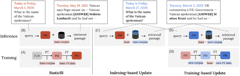
Figure 1: Task Framework of DynamicIR. This figure shows the training and inference process of DynamicIR for each setup. We differentiate each model by color. First, in StaticIR, (A) retrieval models are pretrained on the base corpus ($C_{\textit{base}}$) and finetuned on the query-document pairs of the base corpus ($R_{\textit{base}}$). During inference (B), they perform retrieval only with the indexed $C_{\textit{base}}$. Second, in Indexing-based Update, (C) we use the same retriever developed from StaticIR and conduct an inference with the indexed $C_{\textit{base}}$ and $C_{\textit{new}}$. Lastly, in Training-based Update, (D) the retriever is continually pretrained on $C_{\textit{new}}$ building upon the pretrained model on $C_{\textit{base}}$. Subsequently, it is finetuned on the combination of $R_{\textit{base}}$ and $R^{\prime}_{\textit{new}}$ and (E) conduct an inference with the indexed $C_{\textit{base}}$ and $C_{\textit{new}}$.

1 Introduction

Transformer-based information retrieval (IR) models play a vital role in advancing the field of semantic document search for information-seeking queries. Notably, Generative Retrieval (GR) (Petroni et al., 2019; De Cao et al., 2020; Wang et al., 2022; Bevilacqua et al., 2022; Tay et al., 2022; Zhou et al., 2022; Lee et al., 2022b, a; Sun et al., 2023; Li et al., 2023b) has recently gained a significant amount of recognition from the research community for its simplicity and high performance However, Dual Encoder (DE) (Gillick et al., 2018; Karpukhin et al., 2020a; Ni et al., 2021; Gao et al., 2022; Izacard et al., 2022; Ram et al., 2022) continues to hold sway in practical IR systems. This contrast underscores the need for an investigation into their practical applicability. However, there is a lack of comprehensive comparison between DE and GR in real-world scenarios where knowledge is continually evolving and efficiency is crucial.

To this end, we develop a task framework called Dynamic Information Retrieval (DynamicIR) where we conduct an extensive analysis utilizing the StreamingQA benchmark Liška et al. (2022) of four recent state-of-the-art retrieval models: Spider Ram et al. (2022) and Contriever Izacard et al. (2022) for DE, and Seal Bevilacqua et al. (2022) and Minder Li et al. (2023b) for GR. In our experimental setup, we explore both (1) indexing-based update : updating only the index without any further pretraining and (2) training-based update : further pretraining the parameters on the new corpora in addition to updating the index (as shown in Figure 1). Furthermore, we perform extensive comparison for the efficiency of each method, taking into consideration the floating-point operations (FLOPs) Kaplan et al. (2020) required for the inference, indexing time, inference latency, and storage footprint.

The findings of our study reveal that GR demonstrates superior practicality over DE in terms of 3 different components: adaptability, robustness, and efficiency. (1) GR exhibits superior adaptability to evolving corpus. GR outperforms DE in both indexing-based update and training-based update with improvements of +13.65% and +4.55% showing minimal signs of forgetting and notable acquisition of new knowledge. (2) GR demonstrates greater robustness in handling data with temporal information. While DE reveals a bias toward lexical overlap of timestamps, showing significant degradation (52.23% $\rightarrow$ 17.40%) when removing the timestamps, GR shows robust retrieval performance. (3) GR requires lower indexing costs and inference flops. DE necessitates re-indexing each time whenever the model is updated. Nontheless, the indexing time itself is much longer than GE, resulting in 6 times of time. In terms of storage footprint, GR requires 4 times less storage by storing the knowledge in its internal parameters. For inference flops, GR has $O(1)$ complexity with respect to corpus size, requiring 10 times less computation per query compared to DE which has $O(N)$ complexity with respect to the corpus size. Though the online inference speed remains a challenge for GR, our paper shows the GR’s potential for future use as a practical IR system.

Our contributions are summarized as follows:

• We formulate Dynamic Information Retrieval (DynamicIR) which involves adapting retrieval models to dynamically changing corpora to better align with real-world scenarios.

• Through in-depth analysis, our study concludes that GR is more capable on the adaptability and robustness toward data with temporal information.

• Computation: When performing a head-to-head comparison of DE and GR, GR exhibits notable advantages especially in inference flops, requiring 10 times less computation by maintaining a constant computational demand regardless of corpus size.

• Memory: The results show GR utilizes 4 times less storage footprint by efficiently storing all documents in its internal parameters, in contrast to DE which stores them separately in vector form from the model.

• Our paper highlights the potential of GR to be used in practical IR systems in the future, demonstrating its practicality, robustness, and efficiency.

2 Related Work

Temporal Information Retrieval.

Temporal information retrieval Kanhabua and Anand (2016) has long been a subject of interest in the field of information retrieval. However, despite significant work on the temporal updating of language models Dhingra et al. (2022), there has been limited focus on temporal information retrieval since the rise of transformer-based models like BERT Devlin et al. (2019) that offer robust contextualized embeddings. One potential reason is the prohibitive computational cost associated with storing the updated entire document embedding made by bi-encoders to incorporate additional knowledge. Recently, Metzler et al. (2021) underscored the importance of the efficient implementation of incremental learning in search models. With the advent of generative retrieval methods, we argue that this challenge warrants renewed attention. Due to their fully parameterized end-to-end architecture, generative models are highly sensitive to parameter updates and tend to overfit on training data, limiting their adaptability to knowledge updates without corresponding model parameter modifications. Addressing this challenge is thus crucial for the broader acceptance and use of generative retrievers through time.

Dual Encoder.

Dual encoder methods Lee et al. (2019); Karpukhin et al. (2020b) refer to a set of model architectures where we project the query and document individually into a fixed sized embedding. By contrastive learning, the projected embeddings of positive documents are learned to be close to the query and negative documents to be far away. Although approximate methods and external modules such as MIPS Shrivastava and Li (2014), FAISS Johnson et al. (2019), and ANCE Xiong et al. (2020) can help the efficiency of those models in inference time, these types of models still fall into the limitation that model-dependent embedding dumps need to be made in an asynchronous fashion, and the information needs to be compressed in a fixed-size embedding vector. As we need both positive and negative labeled passages to train dual encoders, some works have tried to navigate these issue by training the model in an unsupervised fashion Izacard et al. (2022); Lee et al. (2019); Sachan et al. (2023).

Generative Retrieval.

Generative retrieval methods initially emerged with the work of De Cao et al. (2020), in which an encoder-decoder model retrieves a document by generating the title of the document from a given query. Tay et al. (2022) introduced DSI, a generative retrieval model that produces a document ID as the output sequence. Building upon DSI, Mehta et al. (2022) adapted it to an additive training setup. However, their work only examined a setting where the output sequence is a document ID, thereby limiting its direct applicability to dynamic retrieval. Wang et al. (2022) and Zhuang et al. (2022) applied query generation, improving DSI’s performance significantly. Rather than mapping to simple numbers for document identifiers, other works explore generating the content itself from documents as identifiers, such as spans Bevilacqua et al. (2022), sentences or paragraphs Lee et al. (2022b), or a mixture of titles, queries, and spans Li et al. (2023b). Other works focus on the broader application of generative retrieval, such as better pretraining objectives for generative retrieval Zhou et al. (2022), multi-hop reasoning Lee et al. (2022b), contextualization of generative retrieval token embeddings for improved performance Lee et al. (2022a), auto-encoder approach for better generalization Sun et al. (2023), and giving ranking signals Li et al. (2023a). Our work builds upon these recent advances in generative retrieval to leverage its potential advantages when concerning temporal information retrieval as we explain below.

3 Dynamic Information Retrieval

Type	Split	Count
Query-Doc pairs	$R_{\textit{base}}$ (2007 – 2019)	99,402
	$R^{\prime}_{\textit{new}}$ (2020)	90,000
Evaluation	$Q_{\textit{base}}$ (2007 – 2019)	2,000
	$Q_{\textit{new}}$ (2020)	3,000
	$Q_{\textit{total}}$ (2007 – 2020)	5,000
Corpus	$C_{\textit{base}}$ (2007 – 2019)	43,832,416
	$C_{\textit{new}}$ (2020)	6,136,419
	$C_{\textit{total}}$ (2007 – 2020)	49,968,835
# Tokens	Base (2007 – 2019)	7.33B
	New (2020)	1.04B
	Total (2007 – 2020)	8.37B
# Tokens per passage	Base (2007 – 2019)	169.7
	New (2020)	167.1
	Total (2007 – 2020)	167.5

Table 1: Statistics of the StreamingQA dataset modified for our setup. # Tokens is the total number of words separated by space in each passage.

3.1 DynamicIR Task Framework

DynamicIR is a task framework that involves adapting the retrieval model to evolving corpora over time. In DynamicIR, we assume that we have a base corpus $C_{\textit{base}}$ and newly introduced corpus $C_{\textit{new}}$, and datasets of query-document pairs $R_{\textit{base}}$ and $R^{\prime}_{\textit{new}}$ from $C_{\textit{base}}$ and $C_{\textit{new}}$, respectively. Unlike $R_{\textit{base}}$, $R^{\prime}_{\textit{new}}$ consists of pseudo-queries, and a detailed explanation is in Section 3.2. We have two types of evaluation set, $Q_{\textit{base}}$ where the answers of the questions are within $C_{\textit{base}}$ and $Q_{\textit{new}}$ where the answers are within $C_{\textit{new}}$. The combination of these sets is denoted as $Q_{\textit{total}}$. As illustrated in Figure 1, DynamicIR consists of three components, (1) StaticIR, (2) Indexing-based updates, and (3) Training-based updates. The latter two parts are for adapting to a new corpus.

StaticIR.

In this part, we focus on retrieving documents only from $C_{\textit{base}}$. The training process begins with pretraining the retriever using $C_{\textit{base}}$, followed by finetuning it with $R_{\textit{base}}$. We evaluate it only on $Q_{\textit{base}}$ with pre-indexed $C_{\textit{base}}$.

Indexing-based Update.

In this setup, we incorporate a new corpus to the retrieval models by indexing it without any parameter updates. We utilize a retrieval model trained in StaticIR, so that this approach is quick and straightforward. We evaluate the retriever on $Q_{\textit{base}}$ and $Q_{\textit{new}}$ with pre-indexed $C_{\textit{base}}$ and $C_{\textit{new}}$.

Training-based Update.

In this advanced setup for update, we continually pretrain the retriever parameters with $C_{\textit{new}}$, building upon a model trained with $C_{\textit{base}}$. Subsequently, we finetune it using a combination of datasets, $R_{\textit{base}}$ and $R^{\prime}_{\textit{new}}$. Similar to indexing-based updates, we evaluate the retriever on $Q_{\textit{base}}$ and $Q_{\textit{new}}$ with pre-indexed $C_{\textit{base}}$ and $C_{\textit{new}}$.

Key considerations to successfully perform retrieval include (1) mitigating catastrophic forgetting of $C_{\textit{base}}$ McCloskey and Cohen (1989); Kirkpatrick et al. (2017), (2) effectively acquiring new knowledge from $C_{\textit{new}}$, (3) minimizing the additional computation required for updates, (4) efficiently compressing and storing information as the size of data continually increases. To summarize, we highlight the importance of striking a balance between retaining existing knowledge and incorporating new information, ensuring computational and memory efficiency.

3.2 Benchmark

To evaluate the performance of retrieval models in a dynamic scenario, we employ StreamingQA Liška et al. (2022) designed for temporal knowledge update. StreamingQA is the benchmark that includes both the timestamps of question and document publication, which is critical for considering the temporal dynamics. Specifically, the format of question is ‘Today is Wednesday, May 6, 2020. [question]’ and for documents, it is ‘Thursday, February 7, 2019. [article text]’. Liška et al. (2022). Moreover, the dataset spans a wide range of information, covering a 14-year period and comprising over 50 million passages, more than double the volume of Wikipedia’s entire content with 21 million passages.

Temporal Information. The StreamingQA comprises a corpus spanning from 2007 to 2020 and supervised dataset of question-document pairs covering the years from 2007 to 2019. In our work, $C_{\textit{base}}$ comprises articles from 2007 to 2019 and $C_{\textit{new}}$ consists of articles from 2020. Similarly, regarding the supervised dataset, $R_{\textit{base}}$ is from 2007 to 2019, $R^{\prime}_{\textit{new}}$ is from 2020. Notably, all questions in the evaluation dataset are asked in 2020, prefixing ‘Today is [Day], [Month Date] , 2020’. For comprehensive evaluation, the StreamingQA has two types of questions, $Q_{\textit{base}}$ for retrieving documents from ${C_{\textit{base}}}$ and $Q_{\textit{new}}$ for retrieving documents from ${C_{\textit{new}}}$.

Modification.

We create modified version of StreamingQA to fit it to our experimental setup. The original StreamingQA dataset lacks query-document pairs from ${C_{\textit{new}}}$, making it challenging to explore training-based updates. To address this, we generate additional 90,000 queries from ${C_{\textit{new}}}$. To make this, we employ a trained model similar to the one used in docT5 query generation. The size of this additional dataset $R^{\prime}_{\textit{new}}$ is similar to that of $R_{\textit{base}}$. Examples of generated dataset are in Table A.4 and details of the query construction are explained at Appendix A.4.

	Performance $(hit@5)$			Efficiency
Evaluation	$Q_{\textit{total}}$	$Q_{\textit{base}}$	$Q_{\textit{new}}$	Inference Flops	Indexing Time	Inference Latency ($T_{\textit{online}}$ / $T_{\textit{offline}}$)	Storage Footprint
StaticIR
Spider	-	19.65%	-	8.9e+10	18.9h	24.48ms / 26m	173.8G
Contriever	-	16.10%	-	8.9e+10	18.9h	212.4ms* / 9.8m	88.8G
[1pt/2pt] SEAL	-	34.95%	-	9.5e+9	2.7h	545.9ms / 1m 5s	34.5G
MINDER	-	37.90%	-	9.5e+9	2.7h	424.6ms / 1m 5s	34.5G
Indexing-based Update
Spider	24.82%	15.60%	34.03%	1.0e+11	20.4h	24.84ms / 28m	196.8G
Contriever	19.66%	13.75%	28.53%	1.0e+11	20.4h	228.8ms* / 10.5m	99.8G
[1pt/2pt] SEAL	33.05%	32.75%	33.50%	9.5e+9	3.1h	612.2ms / 1m 26s	37.5G
MINDER	38.47%	37.65%	39.70%	9.5e+9	3.1h	485.4ms / 1m 26s	37.5G
Training-based Update
Spider	36.99%	21.75%	52.23%	1.0e+11	20.4h	24.84ms / 28m	196.8G
Contriever	23.85%	8.20%	39.50%	1.0e+11	20.4h	228.8m* / 10.5m	99.8G
[1pt/2pt] SEAL†	41.01%	38.25%	43.77%	9.5e+9	3.1h	612.2ms / 1m 26s	37.5G
MINDER†	41.54%	38.85%	44.23%	9.5e+9	3.1h	485.4ms / 1m 26s	37.5G

• We employ LoRA during the continual pretraining and apply it to DE for the next revision.

• For Contriever, we measure $T_{\textit{online}}$ using faiss-cpu.

Table 2: Results of DynamicIR. Our experiments are divided into 3 setups, (1) StaticIR, (2) Indexing-based Updates, and (3) Training-based Updates. For each setups, we assess the performance on $Q_{\textit{total}}$, $Q_{\textit{base}}$, and $Q_{\textit{new}}$, and efficiency which is evaluated using 4 metrics. We highlight the best scores in bold for each setup. For Inference Latency, $T_{\textit{online}}$ indicates the time required for query embeddings and search, and $T_{\textit{offline}}$ indicates the time required for loading the indexed corpus. Additionally, the zero-shot performance for all models is provided in Appendix 7.

4 Experimental setup

4.1 Retrieval Models

Dual-Encoder (DE)

We select Spider Ram et al. (2022) and Contriever Izacard et al. (2022) as representative for DE. Since our experiments include a pretraining stage to store the corpus itself, we use baselines that focus more on the pretraining methods. As Spider does not include a method for the finetuning stage, we use DPR Karpukhin et al. (2020a) and adhere to its original training scheme such as utilizing in-batch negative training.

Generative Retrieval (GR)

We select SEAL  Bevilacqua et al. (2022) that employs the substrings in a passage as document identifiers and MINDER Li et al. (2023b) that uses a combination of the titles, substrings, and pseudo-queries as identifiers. We choose the two as baselines since unlike other GR models using document IDs as identifiers Tay et al. (2022); Wang et al. (2022), SEAL and MINDER can lead to more effective updates of individual pieces of knowledge by autoregressively generating the context.

4.2 Evaluation

We assess retrieval performance with three evaluation dataset, $Q_{\textit{base}}$, $Q_{\textit{new}}$, and $Q_{\textit{total}}$. First, we evaluate the retention of existing knowledge by 2,000 questions that should be answered from the $C_{\textit{base}}$. Second, we assess the acquisition of new knowledge by 3,000 questions that should be answered from $C_{\textit{new}}$. Both sets of 5,000 questions are randomly extracted from the entire evaluation data of StreamingQA, maintaining the ratio (16.60%) of each question type for existing knowledge and new knowledge. Finally, we assess total performance by calculating the unweighted average of the above two performance. Furthermore, we measure computational and memory efficiency to assess the practicality of retrieval models. We provide metrics used to evaluate both performance and efficiency in following Section 4.3.

4.3 Metric

4.3.1 Performance

Hit@5. It measures whether the gold-standard passage is included in the top 5 retrieved passages. Most document search systems do not limit results to one or provide too many; we consider 5 to be a reasonable number for assessment. The full results of Hit@N, where N is set to 5, 10, 50, and 100, are in Table 10.

Answer Recall.

It measures whether the retrieved passage contains an exact lexical match for the gold-standard answer. The results using this metric are in Table 11.

4.3.2 Efficiency

Inference FLOPs.

Inference flops (Floating Point Operations) is the number of floating-point arithmetic calculations during inference. We measure flops per instance using $DE_{\textit{flops}}$ for DE and $GR_{\textit{flops}}$ for GR.

$$DE_{\textit{flops}} =C\times IP_{\textit{flops}}$$

$$GR_{\textit{flops}} =FW_{\textit{flops}}^{\textit{enc}}+L\times Beam_{\textit{flops}}$$

$$IP_{\textit{flops}} =d_{\text{model}}\times(d_{\text{model}}-1)$$

$$FW_{\textit{flops}} =2N+2n_{\text{layer}}n_{\text{ctx}}d_{\text{attn}}$$

$$Beam_{\textit{flops}} =FW_{\textit{flops}}^{\textit{dec}}\times IP_{\textit{flops}}\times|V|\log|V|\times B$$

where $C$ is the corpus size, $L$ is the sequence length of output, $d_{\textit{model}}$ is dimension of hidden vector, $N$ is the model size, $n_{layer}$ is the number of layers, $n_{ctx}$ is the length of input context, $d_{attn}$ is the dimension of attention, $V$ is the vocab size, and $B$ is the beam size. $|V|log|V|$ is the complexity of obtaining possible token successors with FM-index Bevilacqua et al. (2022). $FW_{\textit{flops}}$ is flops for the forward pass of the transformer which is defined from Kaplan et al. (2020) and we apply it to both encoder and decoder.

Indexing Time.

There is a difference in the concept of indexing between DE and GR. In the case of DE, indexing involves embedding, which converts the corpus into representations using encoder. In GR, conversely, indexing refers the data processing of document identifiers to constrain beamsearch decoding, ensuring the generation of valid identifiers. Specifically, for our GR models using FM-index, the indexing process involves compressing the full-text substrings, since they use all n-grams in a passage as possible identifiers Bevilacqua et al. (2022).

Inference Latency.

Inference is divided into two main stages: (1) loading a pre-indexed corpus and (2) retrieving, which includes query embedding and search. We classify the former as offline latency because, after the initial loading, subsequent operations mainly involve the second part. Thus, the latter, considered the most crucial part, is referred to as online latency. In our study, we measure both for more practical analysis.

Storage Footprint.

We measure the storage footprint of both the retrieval model and the pre-indexed corpus, which is required for performing retrieval.

5 Experimental Results

In this section, we present the results of assessing DE and GR, focusing on their practicality in three setups. Section 5.1 shows the performance of the models in both static and dynamic settings, while Section 5.2 shows their efficiency.

5.1 Performance of DynamicIR

StaticIR.

As shown in Table 2, our evaluation on $Q_{\textit{base}}$ reveals that GR significantly outperforms DE in hit@5, which corroborates the results of prior work. Specifically, SEAL and MINDER achieve 34.95% and 37.90%, while Spider and Contriever achieve 19.65% and 16.10%, demonstrating superior performance with an average improvement of +18.55%.

Indexing-based Update.

The results show that GR significantly outperforms DE in hit@5 with average improvements of +13.52%, +20.53%, and +5.32% in $Q_{\textit{total}}$, $Q_{\textit{base}}$, and $Q_{\textit{new}}$ respectively.

When examining the performance of $Q_{\textit{base}}$ compared to its performance in StaticIR for checking forgetting issues, we observe a slight degradation for both GR and DE. GR experiences a 1.23% decrease (36.43% $\rightarrow$ 35.20%), while DE experiences a 2$\times$ larger decline of 3.2% (17.88% $\rightarrow$ 14.68%) on average of each model. This observation suggests that GR is more robust in retaining existing knowledge.

In assessment using $Q_{\textit{new}}$, GR models achieve higher performance than that of $Q_{\textit{base}}$ (36.60% and 36.43% for $Q_{\textit{new}}$ and $Q_{\textit{base}}$ on average of each model), indicating its remarkable generalizability. Surprisingly, however, as illustrated in Figure 2, DE models display a considerable performance gap between $Q_{\textit{new}}$ and $Q_{\textit{base}}$. The performance of DE on $Q_{\textit{new}}$ surpasses that of $Q_{\textit{base}}$ by more than 2 times (31.28% and 14.68% for $Q_{\textit{new}}$ and $Q_{\textit{base}}$ on average). This observation appears unusual, especially when considering that the models are only trained on $C_{base}$ and $R_{\textit{base}}$. Regarding this phenomenon, we identify an undesired bias in DE models towards lexical overlap of timestamp. As shown in Table 3, when bias-inducing factor is removed, the performance of $Q_{\textit{new}}$ significantly decreases to a level similar to the performance on $Q_{\textit{base}}$ (32.28% $\rightarrow$ 12.84% on average). We provide a detailed analysis for this in Section 6.

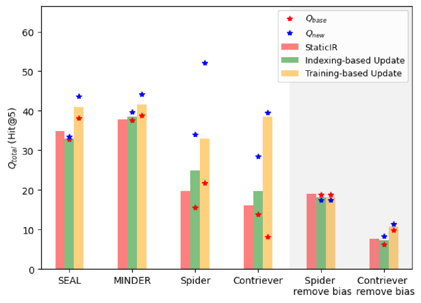
Figure 2: The figure highlights the gap between $Q_{\textit{base}}$ and $Q_{\textit{new}}$ compared to GR. Additionally, it depicts the decrease in $Q_{\textit{new}}$ when the bias-inducing factor is eliminated.

Training-based Update.

As shown in Table 2, our results show that overall, training-based updates are more beneficial for adaptation compared to indexing-based updates for both DE and GR.

	$Q_{\textit{new}}$ in Indexing-based Updates		$Q_{\textit{new}}$ in Training-based Updates
	original query	timestamp-removed query	original query	timestamp-removed query
Spider	34.03%	17.40%	52.23%	17.40%
Contriever	28.53%	8.27%	39.50%	11.43%
SEAL	33.50%	37.50%	43.77%	39.53%
MINDER	39.70%	39.47%	44.23%	41.73%

Table 3: Ablation Study on the Bias of DE with regard to $Q_{\textit{new}}$. DE shows a lexical bias toward temporal information on $Q_{\textit{new}}$ where all queries are asked in 2020 and the gold documents are published also in 2020. When removing the timestamp of asked query, the performance drastically drops by more than 2 – 3 times, while GR does not exhibit noticeable changes.

Specifically, on $Q_{\textit{base}}$, GR achieves even higher performance compared to its performance in StaticIR, showing an improvement of +2.12% (36.43% $\rightarrow$ 38.55%) without exhibiting any signs of forgetting. We conjecture that as GR leverages the attributes of language models for learning language distributions, it derives advantages from training on an expanded volume of in-domain data, leading to the mitigation of the forgetting issue. In contrast, DE experiences an average decrease of 2.90% (17.88% $\rightarrow$ 14.98%), with large degradation in Contriever and a slight gain in Spider, indicating a weaker ability to retain existing knowledge compared to GR.

When evaluating the models on $Q_{\textit{new}}$, all models showcase superior adaptability to new knowledge compared to indexing-based updates, with an average improvement of +7.40% for GR and +14.00% for DE. However, a similar phenomenon to that observed in indexing-based updates becomes apparent, where the performance gap between $Q_{\textit{base}}$ and $Q_{\textit{new}}$ in DE models is significant by more than 2 – 4 times. The issue of abnormally high performance on $Q_{\textit{new}}$ also stems from bias toward temporal information. when we eliminate query timestamp, the performance of $Q_{\textit{new}}$ significantly drops by more than 3 times (45.87% $\rightarrow$ 14.42% on average)

Please note that for fully parametric GR models, SEAL and MINDER, we apply LoRA Hu et al. (2021) during the pretraining phase to facilitate the efficient adaptation to a new corpus. We extend application of LoRA to feed-forward network modules, leading to improved adaptability. A detailed analysis is provided in Section 6.

5.2 Computational and Memory Efficiency

Indexing Time.

Our results reveal that DE models incur significantly higher time costs compared to its GR counterparts during the indexing of all documents. Specifically, GR takes 2.7 hours for $C_{base}$, while DE requires 18.9 hours, highlighting more than 6$\times$ speed advantage for GR. When incorporating $C_{new}$, the time increases to 3.1 hours for GR and 20.4 hours for DE.

The crucial aspect is that DE models necessitate re-indexing the entire corpus, irrespective of the corpus update. In contrast, GR models have a significant advantage in that they do not require re-indexing when the model is changed. This issue becomes even more prominent when the corpus size is substantial or increases, which is a common occurrence in practical applications like search engines, handling vast and ever-changing collections of web documents.

Storage Footprint.

When evaluating over storage footprint, we could see GR has notably reduced storage requirements. For DE, the average storage allocation is 127Gfor the indexed base corpus and 3.8G for the retrieval model. In contrast, GR models exhibit significantly lower figures, with 29G and 5.5G, respectively, requiring 4$\times$ less memory than DE. Notably, the memory requirements for DE models are directly affected by the corpus size, as they store representations of all documents in vector form outside the model. In contrast, GR models have minimal dependence on the corpus size by storing knowledge in their internal parameters.

In terms of information theory, focusing on the efficiency of storing information, GR stores information approximately 4$\times$ more efficiently per passage. Specifically, we incorporates 6M new passages to the retrieval model using only 3.1M parameters (using LoRA) and an extra 3GB FM-index for fully parametric GR models in training-based updates. As a result, when using FP16, GR models necessitate approximately 501 bytes of storage per passage. This calculation considers 1 byte stored in the retrieval model and an additional 500 bytes stored in the FM-index. In contrast, DE demands 2,048 bytes for storing information in indexed representations with a dimension of 1,024. However, we note that the index of DE is often quantized to FP8 or higher.

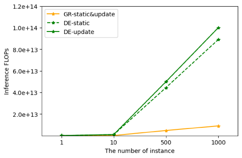
Figure 3: Inference FLOPs according to the number of instances. The flops for GR on both the static and updated corpus are identical, as it maintains consistent flops regardless of the corpus size. Conversely, DE shows variations in flops depending on the corpus size. Also, as the number of instance increases, the required flops increase significantly.

Inference Flops.

Our results in Table 2, GR models require 10 less computation per instance exhibiting 9.5e+9 for the all three setups while DE models have 8.9e+10 and 1.0e+11 for StaticIR and DynamicIR, respectively. GR has $O(1)$ complexity regardless of corpus size. As shown in Figure 3, leveraging this advantage, as the corpus size or the number of instances increases, GR yields greater benefits compared to DE. In contrast, DE models, which have $O(N)$ complexity, show a significant increase in inference flops, not only with the growing number of instances but also as the corpus size increases (DE-static vs DE-update). The process of performing the inner product for all documents each time highly demands on computational resources.

Inference Latency.

In this section, we describe the results of inference latency which is critical especially in applications where quick response times are important. According to Table 2, for offline latency, GR models surpass their DE counterparts, achieving a speed more than 10 – 20 times faster. This is due to GR’s requirement of loading only the compressed corpus, FM-index, while DE needs to upload all passage representations. For online latency, however, GR is 20 times slower than DE using faiss-gpu. Despite DE requiring 10 times more inference flops, it seems that the FAISS module contributes significantly to the inference speed of DE.

While inference speed remains a challenge in GR, we anticipate that with the advent of powerful computing resources or the development of efficiency-focused modules, such as FAISS Johnson et al. (2019), GR could be considered valuable enough to use as a practical IR system in the future. This belief is based on its noteworthy advantages in inference flops, memory, and overall high performance and robustness.

6 Analysis

DE’s bias toward lexical overlap of timestamp.

Our findings in DynamicIR reveal a noteworthy phenomenon related to DE models, showcasing significantly superior performance on $Q_{\textit{new}}$ compared to $Q_{\textit{base}}$ by more than 2 times. This occurs not only in training-based updates but also in indexing-based updates that the models never encounter a new corpus during training. The cause of this phenomenon is identified in the characteristics of the evaluation data. All timestamps in the queries are set to the year 2020 and all timestamps in the documents within the new corpus are also in the year 2020. This suggests that DE models may exhibit an undesirable bias towards lexical overlap. In this context, to clarify the bias of DE models towards temporal information, we finetune the models using dataset that query dates are removed. Subsequently, we evaluate the models using evaluation dataset that query dates are eliminated. This experimental approach is viable because, among the total 5,000 evaluation instances, only 7 cases require retrieving different passages for the same questions but with different timestamps as depicted Figure 1. In Table 3, our results show that when evaluated with a timestamp-removed dataset, the performance on $Q_{\textit{new}}$ is significantly degraded in DE models, whereas GR models exhibit stable performance. For this analysis, we identify that the unusually high performance of DE stems from the bias of lexical overlap with timestamp.

Model	$R^{\prime}_{\textit{new}}$	$Q_{\textit{total}}$	$Q_{\textit{base}}$	$Q_{\textit{new}}$
Spider	with	36.99%	21.75%	52.23%
	w/o	35.77%	29.90%	41.63%
[1pt/1.7pt] Contriever	with	23.85%	8.20%	39.50%
	w/o	19.12%	13.90%	24.33%
SEAL	with	41.01%	38.25%	43.77%
	w/o	37.91%	37.25%	38.90%
[1pt/1.7pt] MINDER	with	41.54%	38.85%	44.23%
	w/o	37.80%	38.15%	40.03%

Table 4: Analysis the effectiveness of $R^{\prime}_{\textit{new}}$ with pseudo-queries in training-based updates. In this table, w/o refers only using $R_{\textit{base}}$ during finetuning. The results show that it is effective to additionally include the $R^{\prime}_{\textit{new}}$.

Effectiveness of finetuning dataset generated from New corpus.

We analyze the effectiveness of utilizing $R^{\prime}_{\textit{new}}$ newly created based on $C_{\textit{new}}$ using docT5.

As shown in Table 4, the utilization of $R^{\prime}_{\textit{new}}$ demonstrates superior performance when compared to the outcomes using only $R_{base}$.

The results indicate that all models experience benefits from using $R_{new}$ on $Q_{\textit{total}}$. In particular, GR models enhance their performance not only on $Q_{\textit{new}}$ but also on $Q_{\textit{base}}$, aligning with previous studies that utilize query generation for GR Mehta et al. (2022); Zhuang et al. (2023); Lin and Ma (2021); Mallia et al. (2021); Cheriton (2019); Wang et al. (2022); Pradeep et al. (2023). However, in the case of DE models, there is a degradation observed on $Q_{\textit{base}}$, indicating the issue of forgetting. Nonetheless, there are significant gains on $Q_{\textit{new}}$, leading to an overall increase in performance on $Q_{\textit{total}}$. By leveraging the attributes of language models for learning language distributions, GR attains superior results when adapting to a new corpus, even on $Q_{\textit{base}}$, within the context of in-domain scenarios.

Model	LoRA	$Q_{\textit{total}}$	$Q_{\textit{base}}$	$Q_{\textit{new}}$
SEAL	$attn+ffn$	38.08%	37.25%	38.90%
	$attn$	31.69%	32.00%	31.37%
MINDER	$attn+ffn$	39.04%	38.15%	39.93%
	$attn$	38.35%	37.50%	39.20%

Table 5: Analysis of effectiveness according to the application range of LoRA. We extend its application to feed-forward network modules beyond attention modules. The results exhibit that activating feed-forward network modules is beneficial, not only for acquiring new knowledge but also for retraining past knowledge.

Layer	Projection	Avg num of DPs
FFN	FC1	1.1M
	FC2	77K
	Total	1.87M
ATTN	Query	41K
	Key	35K
	Total	76K

Table 6: Average number of Dynamic Parameters (DPs), the parameters that have large impact on acquiring new knowledge, per block. It reveals that DPs are significantly more prevalent in the fully connected layer, exceeding those in the attention layer by more than 2$\times$

The Effectiveness of LoRA on Feed-Forward Network.

For fully-parametric GR models, we employ LoRA to efficiently conduct continual pretraining on a new corpus. In order to better target key parameters for incorporating new knowledge when utilizing LoRA, we extend its application to feed-forward network modules. As shown in table 5, it proves to be more effective when applied to both attention and feed-forward network modules than when applied only to attention modules. To achieve this, we initially analyze which parameters undergo the most significant change during the acquisition of new knowledge using the SEAL model.

Specifically, we calculate absolute differences of parameters between the model trained on the existing corpus and the continually trained model on the new corpus with full parameters. After that, we determine parameters exceeding the 90th percentile of these absolute differences, and we call them Dynamic Parameters (DPs). As shown in Table 6, our analysis reveals that DPs are significantly more prevalent in the fully connected layer, exceeding those in the attention layer by more than 2 times. As a result, expanding LoRA to feed-forward networks is beneficial for adapting to a new corpus.

7 Conclusion

In this work, we conduct an extensive comparison of DE and GR in terms of practicality in DynamicIR framework. Our results demonstrate GR exhibits superior performance, robustness, and efficiency compared to DE which is widely used in practical IR systems. Although online inference latency of GR remains the challenge, it has potential as a practical IR system in the future, when given its high adaptability to evolving knowledge, robustness in handling data characteristics, lower memory requirements by storing knowledge in its internal parameters, and efficiency in terms of inference flops and indexing time. In this paper, we shed light on the practicality of GR.

Appendix A Appendix

Model	$Q_{\textit{total}}$	$Q_{\textit{base}}$	$Q_{\textit{new}}$
Spider	13.28%	8.95%	17.60%
Contriever	18.74%	7.15%	30.33%
SEAL	20.60%	19.80%	21.40%
MINDER	25.87%	25.00%	26.73%

Table 7: The zero-shot performance on updated corpora. It demonstrates the zero-shot performance achieved without further training from released checkpoints. Overall, it exhibits a similar trend to our models trained on StreamingQA dataset.

A.1 Zero-shot performance of DE and GR

We conduct zero-shot experiments to assess the base performance of retrieval models on StreamingQA, utilizing Spider trained on NQ, Contriever trained on CCNet and Wikipedia, SEAL trained on KILT, and MINDER trained NQ. The results of the zero-shot experiments are presented in in Table 7.

A.2 Implementation Details

A.2.1 Dual Encoder

Spider.

Spider experiments are conducted using 8x A100 80GB GPUs, and our implementation setup is primarily based on Spider. SPIDER Ram et al. (2022) code. We employ the bert-large-uncased pretrained model from HuggingFace, with fp16 enabled and weight sharing, configuring a batch size of 512 and a maximum sequence length of 240. For the pretraining stage, we run a full epoch with a learning rate of 2e-05 and a warm-up of 2,000 steps. The pretraining data is made by running the spider code on the provided documents from StreamingQA. This yields 95,199,412 pretraining data from base corpus and 21,698,933 from new corpus, which are used for StaticIR and DynamicIR, respectively. It takes about 5 days for pretraining the base model and 25 hours for continual pretraining the updated model. For the finetuning stage, we run for maximum 10 epochs with learning rate of 1e-05 and warm-up of 1,000 steps with batch size of 512. We select the best checkpoint with lowest validation loss.

Contriever.

Contriever experiments are done on 4x A100 40GB GPUs. We employ bert-large-uncased pretrained model and follow the paper Izacard et al. (2022) and their official codebase for the implementation and hyperparameter setup. We adjust the per_gpu batch size from 256 to 64 to fit in our gpu resource. Total step size is 110,000 for base (warmup 4,000 steps) and 16,000 (warmup 1,000 steps) for continual pretraining on $C{new}$, which is equivalent to one epoch. Learning rate is set to 1e-04. For the finetuning stage, we run contriever for maximum 10 epochs (about 8000 steps, warmup for 100 steps) with eval frequency of 200 steps and select the checkpoint with lowest eval loss. The per_gpu batch size is set to 32. All the hyperparemeters are the same with the pretraining setup, except the ones mentioned above.

A.2.2 Generative Retrieval

SEAL.

We employ the bart-large pre-trained model for GR and train the model in Fairseq framework for using SEAL.Bevilacqua et al. (2022). Due to this context, when we utilize LoRA method, we implement the method within the Fairseq framework. For the pretraining stage of the base retrieval model in StaticIR, we generate 2 random spans and 1 full passage with the publication timestamp as input for each instance using the past corpus, resulting in 130,897,221 (130M) unsupervised data. We train the initial model on 16x A100 40GB GPUs with a batch size of 7,400 tokens and a learning rate of 6e-5. Subsequently, for the finetuning stage in StaticIR using $R_{\textit{base}}$, we use 10 random spans as document identifiers per question, resulting in 994,020(994K). We train this model using 4x A100 80GB GPUs with batch size of 11,000tokens and a learning rate of 6e-5. In the continual pretraining stage for the updated model in training-based updates of DynamicIR, we use 3 random spans and 1 full passage with the publication timestamp as input for each instance, utilizing the updated corpus, which results in 24,471,541 (24M) unsupervised data. We train this updated model using 4x A100 80GB GPUs with a batch size of 11,000 tokens and a learning rate of 1e-4. Subsequently for finetuning stage in training-based update of DynimicIR using $R_{\textit{base}}$ and $R^{\prime}_{\textit{new}}$, we generate 10 random spans as passage identifiers per question, respectively, resulting in 1,894,020(1.8M) data.

MINDER.

We use 2x A100 80GB GPUs for MINDER experiments. We use the pretrained model which is used for SEAL experiments, since MINDER has identical pretraining process to that of SEAL. For retrieval model of StaticIR, we create MINDER-specific data comprising of 10 spans and 5 pseudo-queries as passage identifiers per question, resulting in 1,491,030(1.4M). For retrieval model of training-based updates in DynamicIR, we generate 10 spans and 5 pseudo-queries, resulting in 2,841,030(2.8M) data. We run all MINDER models for maximum 10 epochs using with max token of 18,000 and a learning rate of 6e-5.

MINDER	$Q_{\textit{total}}$	$Q_{\textit{base}}$	$Q_{\textit{new}}$
w/o title	41.54%	38.85%	44.23%
with pseudo-title	40.86%	38.15%	43.57%

Table 8: MINDER with and without Titles as Identifiers. The results indicate that there is little difference between the use of identifiers with and without the title.

A.3 Difference in the presence of Titles as Identifiers for MINDER

The original MINDER model employs three components, titles, substrings, and pseudo-queries, as its identifiers. However, as the StreamingQA dataset lacks title information, we exclude document titles when constructing the MINDER model. To investigate the impact of this omission on performance, we conduct an analysis within training-based updates by fine-tuning utilizing pseudo-queries generated by GPT-3.5. Our results demonstrate that the omission of titles, in comparison to the utilization of pseudo-titles, has a negligible impact on performance as shown in Table 8.

A.4 Constructing the query-document pairs from new corpus

Reflecting the original evaluation dataset’s distribution which balanced similar proportions of new (2020) and base ( 2019) data, we replicate this distribution in our query generation based on new corpus. We randomly selected 90,000 passages from the 6 million 2020 passages. Subsequently, we finetuned a T5-base model on the query-document pairs from StreamingQA’s base corpus, applying a hyperparameter configuration similar to docT5 query generation, feeding date-prefixed passages as input and producing date-prefixed queries as output. The training process comprises three epochs, with each taking roughly 45 minutes on an NVIDIA A6000 GPU. We then use the trained T5 model to generate one pseudo-query for each of the 90,000 selected passages, a process lasting approximately 90 minutes. Ensuring alignment with our study’s temporal focus, we verify that the date information in the generated queries corresponded to 2020. Following a manual adjustment to ensure the queries are asked in 2020, we assemble the queries and corresponding documents into an additional finetuning dataset for the retrieval models, a process that takes about four hours in total. Examples of the finetuning dataset are in Table A.4.

Pseudo-Query	Gold Passage
Today is Sunday, October 25, 2020. When did the pay gap between Pakistani employees and white employees decrease to 2%?	Monday, October 12, 2020. In 2019 median hourly earnings for white Irish employees were 40. 5% higher than those for other white employees at 17.55, while Chinese workers earned 23.1% more at 15.38 an hour and Indian workers earned 14.43 an hour - a negative pay gap of 15.5%. Annual pay gap Breaking down the data by gender, the ONS said ethnic minority men earned 6.1% less than white men while ethnic minority women earned 2.1% more than white women. The ONS added that ethnicity pay gaps differed by age group. Ämong those aged 30 years and over, those in ethnic minority tend to earn less than those of white ethnicities,ït said. In contrast, those in the ethnic minority group aged 16 to 29 years tend to earn more than those of white ethnicities of the same age. Gender pay gap The ONS found that the pay gap of 16% for Pakistani employees aged more than 30 shrank to 2% for those aged 16-29.
Today is Sunday, May 2, 2020. What was the top level of the FTSE 100?	Tuesday, April 28, 2020. But the big weekly shop has made a comeback, with the amount families spend on an average shopping trip hitting a record high. The new tracking data comes after Tesco boss Dave Lewis said the pandemic had changed people’s shopping habits, which he said have r̈everted to how they were 10 or 15 years ago.M̈eanwhile, is this the end of loo roll wars? Spaghetti hoops have overtaken lavatory paper as the most out-of-stock item in Britain’s stores. Follow our guide to minimising your risk of catching Covid-19 while shopping. The oil giant said there would continue to be an ëxceptional level of uncertaintyïn the sector. Meanwhile, the FTSE 100 soared to a seven-week high. Follow live updates in our markets blog.
Today is Tuesday, March 24, 2020. Why did President Trump sign an executive order banning hoarding?	Tuesday, March 24, 2020. President Donald Trump signs executive order banning hoarding March 23 (UPI) – President Donald Trump on Monday signed an executive order to prevent hoarding and price gouging for supplies needed to combat the COVID-19 pandemic. During a briefing by the White House Coronavirus Task Force, Trump and Attorney General William Barr outlined the order which bans the hoarding of vital medical equipment and supplies including hand sanitizer, face masks and personal protection equipment. Ẅe want to prevent price gouging and critical health and medical resources are going to be protected in every form,T̈rump said. The order will allow Health and Human Services Secretary Alex Azar to designate certain essential supplies a s scarce, which will make it a crime to stockpile those items in excessive quantities. Barr said the limits prohibit stockpiling in amounts greater than r̈easonable personal or business needsör for the purpose of selling them in ëxcess of prevailing market pricesädding that the order is not aimed at consumers or businesses stockpiling supplies for their own operation. Ẅe’re talking about people hoarding these goods and materials on an industrial scale for the purpose of manipulating the market and ultimately deriving windfall profits,ḧe said.
Today is Tuesday, November 27, 2020. What is the name of the radio channel Joe Biden was on?	Monday, November 16, 2020. ’Heal the damage’: Activists urge Joe Biden to move beyond b̈order securityÄs Joe Biden prepares to take office, activists say the president-elect must not only take mean ingful action to stabilize the US-Mexico border, but also reckon with his own history of militarizing the border landscape and communities. Biden has promised to end many of the Trump administration’s border policies, but has yet to unveil the kind of bold immigration plan that would suggest a true departure from Obama-era priorities. Cecilia Muoz, Obama’s top immigration adviser who memorably defended the administration’s decision to deport hundreds of thousands of immigrants, was recently added to Biden’s transition team. Biden has stated that he will cease construction of the border wall, telling National Public Radio in August that there will be n̈ot another foot of wall,änd that his administration will close lawsuits aimed at confiscating land to make way for construction. His immigration plan will also rescind Trump’s declaration of a n̈ational emergencyön the southern border, which the Trump administration has used to siphon funds from the Department of Defense to finance construction, circumventing Congress in an action recently declared illegal by an appeals court. Some lawmakers along the border find these developments heartening, after Trump’s border wall construction has devastated sensitive ecosystems, tribal spaces, and communities, a nd has been continuously challenged in court.

Table 9: Examples of Finetuning dataset $R^{\prime}_{new}$ created by docT5.

A.5 Full performance on Hit and Answer Recall

We present the full results of evaluating the performance of DE and GR in both StaticIR and DynamicIR (indexing-based updates and training-based updates). We employ Hit@N and Answer Recall@N metrics, where N is set to 5, 10, 50, and 100, to assess retrieval performance. The results are in Table 10 and Table 11 for Hit and Answer Recall, respectively.

		hit@5				hit@10				hit@50				hit@100
Model	Method	Total	Base	New		Total	Base	New		Total	Base	New		Total	Base	New
Spider	StaticIR	$19.65$	$19.65$	–		$25.40$	$25.40$	–		$38.20$	$38.20$	–		$44.50$	$44.50$	–
	Index-based Update	$24.82$	$15.60$	$34.03$		$30.67$	$20.20$	$41.13$		$44.92$	$32.80$	$57.03$		$51.28$	$38.45$	$64.10$
	Train-based Update	$36.99$	$21.75$	$52.23$		$43.74$	$26.95$	$60.53$		$58.75$	$40.40$	$77.10$		$64.84$	$46.95$	$82.73$
Contriever	StaticIR	$16.10$	$16.10$	–		$20.25$	$20.25$	–		$33.80$	$33.80$	–		$40.90$	$40.90$	–
	Index-based Update	$21.14$	$13.75$	$28.53$		$25.17$	$17.35$	$36.90$		$39.44$	$29.45$	$54.43$		$46.26$	$35.65$	$62.17$
	Train-based Update	$23.85$	$8.20$	$39.50$		$29.26$	$10.55$	$47.97$		$43.66$	$20.35$	$66.97$		$49.64$	$25.35$	$73.93$
SEAL	StaticIR	$34.95$	$34.95$	–		$41.80$	$41.80$	–		$57.25$	$57.25$	–		$63.10$	$63.10$	–
	Index-based Update	$33.13$	$32.75$	$33.50$		$39.64$	$38.90$	$40.37$		$54.14$	$54.50$	$53.77$		$59.71$	$60.55$	$58.87$
	Train-based Update	$41.01$	$38.25$	$43.77$		$47.99$	$45.30$	$50.67$		$62.90$	$60.20$	$65.60$		$67.79$	$65.00$	$70.57$
MINDER	StaticIR	$37.90$	$37.90$	–		$45.00$	$45.00$	–		$59.60$	$59.60$	–		$64.00$	$64.00$	–
	Index-based Update	$38.68$	$37.65$	$39.70$		$45.27$	$44.40$	$46.13$		$60.87$	$60.60$	$61.13$		$66.13$	$66.35$	$65.90$
	Train-based Update	$41.54$	$38.85$	$44.23$		$48.29$	$45.60$	$50.97$		$63.12$	$60.80$	$65.43$		$68.43$	$66.25$	$70.60$

Table 10: Full results on the Hit of DE and GR.

		answer recall @5				answer recall @10				answer recall @50				answer recall @100
Model	Method	Total	Base	New		Total	Base	New		Total	Base	New		Total	Base	New
Spider	StaticIR	$37.55$	$37.55$	–		$47.45$	$47.45$	–		$67.65$	$67.65$	–		$74.80$	$74.80$	–
	Index-based Update	$44.24$	$33.45$	$55.03$		$52.93$	$41.50$	$64.37$		$70.77$	$61.70$	$79.83$		$76.68$	$69.20$	$84.17$
	Train-based Update	$55.79$	$41.05$	$70.53$		$64.32$	$49.90$	$78.73$		$79.25$	$68.90$	$89.60$		$83.63$	$75.50$	$91.77$
Contriever	StaticIR	$28.90$	$28.90$	–		$37.60$	$37.60$	–		$60.20$	$60.20$	–		$68.25$	$68.25$	–
	Index-based Update	$31.34$	$25.15$	$40.63$		$41.84$	$34.80$	$52.40$		$63.05$	$55.15$	$74.90$		$70.98$	$64.30$	$81.00$
	Train-based Update	$37.14$	$20.15$	$54.13$		$46.54$	$28.15$	$64.93$		$66.21$	$48.65$	$83.77$		$72.33$	$56.85$	$87.80$
SEAL	StaticIR	$58.25$	$58.25$	–		$66.30$	$66.30$	–		$80.45$	$80.45$	–		$83.60$	$83.60$	–
	Index-based Update	$55.85$	$56.80$	$54.90$		$63.68$	$64.45$	$62.90$		$77.58$	$78.95$	$76.20$		$81.49$	$82.75$	$80.23$
	Train-based Update	$62.44$	$59.95$	$64.93$		$70.25$	$68.10$	$72.40$		$81.65$	$80.30$	$83.00$		$85.02$	$84.10$	$85.93$
MINDER	StaticIR	$59.50$	$59.50$	–		$68.10$	$68.10$	–		$80.35$	$80.35$	–		$83.75$	$83.75$	–
	Index-based Update	$54.23$	$54.45$	$54.00$		$62.96$	$63.75$	$62.17$		$76.54$	$78.00$	$75.07$		$79.79$	$81.20$	$78.37$
	Train-based Update	$56.74$	$55.35$	$58.13$		$64.45$	$63.70$	$65.20$		$77.19$	$77.40$	$76.97$		$80.34$	$80.50$	$80.17$

Table 11: Full results on the Answer Recall of DE and GR.

References

- Bevilacqua et al. (2022) Michele Bevilacqua, Giuseppe Ottaviano, Patrick Lewis, Wen tau Yih, Sebastian Riedel, and Fabio Petroni. 2022. Autoregressive search engines: Generating substrings as document identifiers. In arXiv pre-print 2204.10628.
- Cheriton (2019) David R. Cheriton. 2019. From doc2query to doctttttquery.
- De Cao et al. (2020) Nicola De Cao, Gautier Izacard, Sebastian Riedel, and Fabio Petroni. 2020. Autoregressive entity retrieval.
- Devlin et al. (2019) Jacob Devlin, Ming-Wei Chang, Kenton Lee, and Kristina Toutanova. 2019. BERT: Pre-training of deep bidirectional transformers for language understanding. In Proceedings of the 2019 Conference of the North American Chapter of the Association for Computational Linguistics: Human Language Technologies, Volume 1 (Long and Short Papers), pages 4171–4186, Minneapolis, Minnesota. Association for Computational Linguistics.
- Dhingra et al. (2022) Bhuwan Dhingra, Jeremy R. Cole, Julian Martin Eisenschlos, Daniel Gillick, Jacob Eisenstein, and William W. Cohen. 2022. Time-aware language models as temporal knowledge bases. Transactions of the Association for Computational Linguistics, 10:257–273.
- Gao et al. (2022) Tianyu Gao, Xingcheng Yao, and Danqi Chen. 2022. Simcse: Simple contrastive learning of sentence embeddings.
- Gillick et al. (2018) Daniel Gillick, Alessandro Presta, and Gaurav Singh Tomar. 2018. End-to-end retrieval in continuous space.
- Hu et al. (2021) Edward J. Hu, Yelong Shen, Phillip Wallis, Zeyuan Allen-Zhu, Yuanzhi Li, Shean Wang, Lu Wang, and Weizhu Chen. 2021. Lora: Low-rank adaptation of large language models.
- Izacard et al. (2022) Gautier Izacard, Mathilde Caron, Lucas Hosseini, Sebastian Riedel, Piotr Bojanowski, Armand Joulin, and Edouard Grave. 2022. Unsupervised dense information retrieval with contrastive learning.
- Johnson et al. (2019) Jeff Johnson, Matthijs Douze, and Hervé Jégou. 2019. Billion-scale similarity search with GPUs. IEEE Transactions on Big Data, 7(3):535–547.
- Kanhabua and Anand (2016) Nattiya Kanhabua and Avishek Anand. 2016. Temporal information retrieval. In Proceedings of the 39th International ACM SIGIR Conference on Research and Development in Information Retrieval, SIGIR ’16, page 1235–1238, New York, NY, USA. Association for Computing Machinery.
- Kaplan et al. (2020) Jared Kaplan, Sam McCandlish, Tom Henighan, Tom B. Brown, Benjamin Chess, Rewon Child, Scott Gray, Alec Radford, Jeffrey Wu, and Dario Amodei. 2020. Scaling laws for neural language models.
- Karpukhin et al. (2020a) Vladimir Karpukhin, Barlas Oğuz, Sewon Min, Patrick Lewis, Ledell Wu, Sergey Edunov, Danqi Chen, and Wen tau Yih. 2020a. Dense passage retrieval for open-domain question answering.
- Karpukhin et al. (2020b) Vladimir Karpukhin, Barlas Oğuz, Sewon Min, Patrick Lewis, Ledell Wu, Sergey Edunov, Danqi Chen, and Wen-tau Yih. 2020b. Dense passage retrieval for open-domain question answering.
- Kirkpatrick et al. (2017) James Kirkpatrick, Razvan Pascanu, Neil Rabinowitz, Joel Veness, Guillaume Desjardins, Andrei A. Rusu, Kieran Milan, John Quan, Tiago Ramalho, Agnieszka Grabska-Barwinska, Demis Hassabis, Claudia Clopath, Dharshan Kumaran, and Raia Hadsell. 2017. Overcoming catastrophic forgetting in neural networks. Proceedings of the National Academy of Sciences, 114(13):3521–3526.
- Lee et al. (2022a) Hyunji Lee, Jaeyoung Kim, Hoyeon Chang, Hanseok Oh, Sohee Yang, Vlad Karpukhin, Yi Lu, and Minjoon Seo. 2022a. Contextualized generative retrieval. arXiv preprint arXiv:2210.02068.
- Lee et al. (2022b) Hyunji Lee, Sohee Yang, Hanseok Oh, and Minjoon Seo. 2022b. Generative multi-hop retrieval. In Proceedings of the 2022 Conference on Empirical Methods in Natural Language Processing, pages 1417–1436.
- Lee et al. (2019) Kenton Lee, Ming-Wei Chang, and Kristina Toutanova. 2019. Latent retrieval for weakly supervised open domain question answering.
- Li et al. (2023a) Yongqi Li, Nan Yang, Liang Wang, Furu Wei, and Wenjie Li. 2023a. Learning to rank in generative retrieval.
- Li et al. (2023b) Yongqi Li, Nan Yang, Liang Wang, Furu Wei, and Wenjie Li. 2023b. Multiview identifiers enhanced generative retrieval.
- Lin and Ma (2021) Jimmy Lin and Xueguang Ma. 2021. A few brief notes on deepimpact, coil, and a conceptual framework for information retrieval techniques.
- Liška et al. (2022) Adam Liška, Tomáš Kočiský, Elena Gribovskaya, Tayfun Terzi, Eren Sezener, Devang Agrawal, Cyprien de Masson d’Autume, Tim Scholtes, Manzil Zaheer, Susannah Young, Ellen Gilsenan-McMahon, Sophia Austin, Phil Blunsom, and Angeliki Lazaridou. 2022. Streamingqa: A benchmark for adaptation to new knowledge over time in question answering models.
- Mallia et al. (2021) Antonio Mallia, Omar Khattab, Nicola Tonellotto, and Torsten Suel. 2021. Learning passage impacts for inverted indexes.
- McCloskey and Cohen (1989) Michael McCloskey and Neal J. Cohen. 1989. Catastrophic interference in connectionist networks: The sequential learning problem. Psychology of Learning and Motivation - Advances in Research and Theory, 24(C):109–165. Funding Information: The research reported in this chapter was supported by NIH grant NS21047 to Michael McCloskey, and by a grant from the Sloan Foundation to Neal Cohen. We thank Sean Purcell and Andrew Olson for assistance in generating the figures, and Alfonso Caramazza, Walter Harley, Paul Macaruso, Jay McClelland, Andrew Olson, Brenda Rapp, Roger Rat-cliff, David Rumelhart, and Terry Sejnowski for helpful discussions.
- Mehta et al. (2022) Sanket Vaibhav Mehta, Jai Gupta, Yi Tay, Mostafa Dehghani, Vinh Q. Tran, Jinfeng Rao, Marc Najork, Emma Strubell, and Donald Metzler. 2022. Dsi++: Updating transformer memory with new documents.
- Metzler et al. (2021) Donald Metzler, Yi Tay, Dara Bahri, and Marc Najork. 2021. Rethinking search. ACM SIGIR Forum, 55(1):1–27.
- Ni et al. (2021) Jianmo Ni, Gustavo Hernández Ábrego, Noah Constant, Ji Ma, Keith B. Hall, Daniel Cer, and Yinfei Yang. 2021. Sentence-t5: Scalable sentence encoders from pre-trained text-to-text models.
- Petroni et al. (2019) Fabio Petroni, Tim Rocktäschel, Patrick Lewis, Anton Bakhtin, Yuxiang Wu, Alexander H. Miller, and Sebastian Riedel. 2019. Language models as knowledge bases?
- Pradeep et al. (2023) Ronak Pradeep, Kai Hui, Jai Gupta, Adam D. Lelkes, Honglei Zhuang, Jimmy Lin, Donald Metzler, and Vinh Q. Tran. 2023. How does generative retrieval scale to millions of passages?
- Ram et al. (2022) Ori Ram, Gal Shachaf, Omer Levy, Jonathan Berant, and Amir Globerson. 2022. Learning to retrieve passages without supervision.
- Sachan et al. (2023) Devendra Singh Sachan, Mike Lewis, Dani Yogatama, Luke Zettlemoyer, Joelle Pineau, and Manzil Zaheer. 2023. Questions are all you need to train a dense passage retriever.
- Shrivastava and Li (2014) Anshumali Shrivastava and Ping Li. 2014. Asymmetric lsh (alsh) for sublinear time maximum inner product search (mips).
- Sun et al. (2023) Weiwei Sun, Lingyong Yan, Zheng Chen, Shuaiqiang Wang, Haichao Zhu, Pengjie Ren, Zhumin Chen, Dawei Yin, Maarten de Rijke, and Zhaochun Ren. 2023. Learning to tokenize for generative retrieval.
- Tay et al. (2022) Yi Tay, Vinh Q. Tran, Mostafa Dehghani, Jianmo Ni, Dara Bahri, Harsh Mehta, Zhen Qin, Kai Hui, Zhe Zhao, Jai Gupta, Tal Schuster, William W. Cohen, and Donald Metzler. 2022. Transformer memory as a differentiable search index.
- Wang et al. (2022) Yujing Wang, Yingyan Hou, Haonan Wang, Ziming Miao, Shibin Wu, Hao Sun, Qi Chen, Yuqing Xia, Chengmin Chi, Guoshuai Zhao, Zheng Liu, Xing Xie, Hao Allen Sun, Weiwei Deng, Qi Zhang, and Mao Yang. 2022. A neural corpus indexer for document retrieval.
- Xiong et al. (2020) Lee Xiong, Chenyan Xiong, Ye Li, Kwok-Fung Tang, Jialin Liu, Paul Bennett, Junaid Ahmed, and Arnold Overwijk. 2020. Approximate nearest neighbor negative contrastive learning for dense text retrieval.
- Zhou et al. (2022) Yujia Zhou, Jing Yao, Zhicheng Dou, Ledell Wu, and Ji-Rong Wen. 2022. Dynamicretriever: A pre-training model-based ir system with neither sparse nor dense index.
- Zhuang et al. (2022) Shengyao Zhuang, Houxing Ren, Linjun Shou, Jian Pei, Ming Gong, Guido Zuccon, and Daxin Jiang. 2022. Bridging the gap between indexing and retrieval for differentiable search index with query generation.
- Zhuang et al. (2023) Shengyao Zhuang, Houxing Ren, Linjun Shou, Jian Pei, Ming Gong, Guido Zuccon, and Daxin Jiang. 2023. Bridging the gap between indexing and retrieval for differentiable search index with query generation.