Subequivariant Graph Reinforcement Learning in 3D Environments
Abstract
Learning a shared policy that guides the locomotion of different agents is of core interest in Reinforcement Learning (RL), which leads to the study of morphology-agnostic RL. However, existing benchmarks are highly restrictive in the choice of starting point and target point, constraining the movement of the agents within 2D space. In this work, we propose a novel setup for morphology-agnostic RL, dubbed Subequivariant Graph RL in 3D environments (3D-SGRL). Specifically, we first introduce a new set of more practical yet challenging benchmarks in 3D space that allows the agent to have full Degree-of-Freedoms to explore in arbitrary directions starting from arbitrary configurations. Moreover, to optimize the policy over the enlarged state-action space, we propose to inject geometric symmetry, i.e., subequivariance, into the modeling of the policy and Q-function such that the policy can generalize to all directions, improving exploration efficiency. This goal is achieved by a novel SubEquivariant Transformer (Set) that permits expressive message exchange. Finally, we evaluate the proposed method on the proposed benchmarks, where our method consistently and significantly outperforms existing approaches on single-task, multi-task, and zero-shot generalization scenarios. Extensive ablations are also conducted to verify our design.
1 Introduction
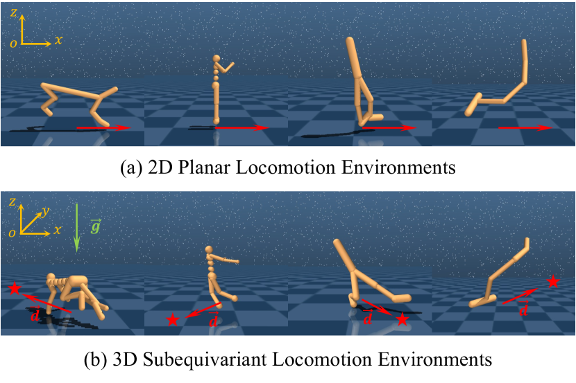
Learning to locomote, navigate, and explore in the 3D world is a fundamental task in the pathway of building intelligent agents. Impressive breakthrough has been made towards realizing such intelligence thanks to the emergence of deep reinforcement learning (RL) (Mnih et al., 2015; Silver et al., 2016; Mnih et al., 2016; Schulman et al., 2017; Fujimoto et al., 2018), where the policy of the agent is acquired through interactions with the environment. More recently, by getting insight into the morphology of the agent, morphology-agnostic RL (Wang et al., 2018; Pathak et al., 2019; Huang et al., 2020; Kurin et al., 2020; Hong et al., 2021; Dong et al., 2022; Trabucco et al., 2022; Gupta et al., 2022; Furuta et al., 2023) has been proposed with the paradigm of learning a local and shared policy for all agents and the tasks involved, offering enhanced performance and transferability, especially in the multi-task scenario. It is usually fulfilled by leveraging Graph Neural Networks (GNNs) (Battaglia et al., 2018) or even Transformers (Vaswani et al., 2017) to derive the policy through passing and fusing the state information on the morphological graphs of the agents.
In spite of the fruitful progress by morphology-agnostic RL, in this work, we identify several critical setups that have been over-simplified in existing benchmarks, giving rise to a limited state/action space such that the obtained policy is unable to explore the entire 3D space. In particular, the agents are assigned a fixed starting point and restricted to moving towards a single direction along the -axis, leading to 2D motions only. Nevertheless, in a more realistic setup as depicted in Figure 1, the agents would be expected to have full Degree-of-Freedoms (DoFs) to turn and move in arbitrary directions starting from arbitrary configurations. To address the concern, we extend the existing environments to a set of new benchmarks in 3D space, which meanwhile introduces significant challenges to morphology-agnostic RL due to the massive enlargement of the state-action space for policy optimization.
Optimizing the policy in our new setup is prohibitively difficult, and existing morphology-agnostic RL frameworks like (Huang et al., 2020; Hong et al., 2021) are observed to be susceptible to getting stuck in the local minima and exhibited poor generalization in our experiments. To this end, we propose to inject geometric symmetry (Cohen & Welling, 2016, 2017; Worrall et al., 2017; van der Pol et al., 2020) into the design of the policy network to compact the space redundancy in a lossless way (van der Pol et al., 2020). In particular, we restrict the policy network to be subequivariant in two senses (Han et al., 2022a): 1. the output action will rotate in the same way as the input state of the agent; 2. the equivariance is partially relaxed to take into account the effect of gravity in the environment. We design SubEquivariant Transformer (Set) with a novel architecture that satisfies the above constraints while also permitting expressive message propagation through self-attention. Upon Set, the action and Q-function could be obtained with desirable symmetries guaranteed. We term our entire task setup and methodology as Subequivariant Graph Reinforcement Learning in 3D Environments (3D-SGRL).
Our contributions are summarized as follows:
-
•
We introduce a set of more practical yet highly challenging benchmarks for morphology-agnostic RL, where the agents are permitted to turn and move in the 3D environments with arbitrary starting configurations and arbitrary target directions. For this purpose, we redesign the agents in current benchmarks by equipping them with more DoFs in a considerate way.
-
•
To effectively optimize the policy on such challenging benchmarks, we propose to enforce the policy network with geometric symmetry. We introduce a novel architecture dubbed Set that captures the rotation/translation equivariance particularly when external force fields like gravity exist in the environment.
-
•
We verify the performance of the proposed method on the proposed 3D benchmarks, where it outperforms existing morphology-agnostic RL approaches by a significant margin in various scenarios, including single-task, multi-task, and zero-shot generalization. Extensive ablations also reveal the efficacy of the proposed ideas.
2 Background
Morphology-Agnostic RL
In the context of morphology-agnostic RL (Huang et al., 2020), we are interested in an environment with agents (a.k.a tasks), where the -th agent comprises limbs that control its motion. At time , each limb of agent receives a state and outputs a torque to its actuator. As a whole, agent executes the joint action to interact with the environment which will return the next state of all limbs and a reward for agent . The goal of morphology-agnostic RL is to learn a shared policy among different agents to maximize the expected return:
| (1) |
where , is a discount factor, and consists of trainable parameters.
The objective in Equation 1 is usually optimized via the actor-critic setup of the deterministic policy gradient algorithm for continuous control (Lillicrap et al., 2016), which estimates the Q-function for agent :
| (2) | ||||
To uniformly learn a shared policy across all agents and tasks, previous methods (Wang et al., 2018; Pathak et al., 2019; Huang et al., 2020; Kurin et al., 2020; Hong et al., 2021; Dong et al., 2022), take into account the interaction of connected limbs and joints, and view the morphological structure of the agent as an undirected graph , where each represents a limb and the edge stands for the joint connecting limb and 111For simplicity, we omit the index and henceforth in the above notations of agent at time , since all agents share the same model for all time, e.g., and .. A graph neural network is then employed to instantiate the policy , which predicts the action given the state of all limbs and the graph topology as input, i.e.,
| (3) |
Equivariance and Subequivariance
To further relieve the difficulty of learning a desirable policy within the massive search space formed by the states and actions of the agent in 3D space, we propose to encode the physical geometric symmetry of the policy learner , so that the learned policy can generalize to operations in 3D, including rotations, translations, and reflections, altogether forming the group of E(). Such constraint enforced on the model is formally described by the concept of equivariance (Thomas et al., 2018; Fuchs et al., 2020; Villar et al., 2021; Satorras et al., 2021; Huang et al., 2022; Han et al., 2022a, b).
Definition 2.1 (E()-equivariance).
Suppose to be 3D geometric vectors (positions, velocities, etc) that are steerable by E(3) transformations, and non-steerable features. The function is E()-equivariant, if for any transformation , , . Similarly, is invariant if .
Built on this notion, Han et al. (2022a) additionally considers equivariance on the subgroup of , induced by the external force like gravity, defined as . By this means, the symmetry is only restrained to the rotations/reflections along the direction of . Such relaxation of group constraint is crucial in environments with gravity, as it offers extra flexibility to the model so that the effect of gravity could be captured. Han et al. (2022a) also presented a universally expressive construction of the -equivariant functions:
| (4) |
where is an Multi-Layer Perceptron (MLP) and is a stack of and along the last dimension. In particular, will reduce to be -equivariant if is omitted in the computation. In this way, can then be leveraged in the message passing process of the graph neural network in Equation 3 to obtain desirable geometric symmetry.
3 Our task and method: 3D-SGRL
In this section, we present our novel formulation for morphology-agnostic RL, dubbed Subequivariant Graph Reinforcement Learning in 3D Environments (3D-SGRL). We first elaborate on the extensions made to the environment in Section 3.1, then introduce our entire framework, consisting of an input processing module (Section 3.2), a novel SubEquivariant Transformer (Set) for expressive information passing and fusion (Section 3.3), and output modules of actor and critic to obtain the final policy and Q-function (Section 3.4).

| 2D-Planar | Our 3D-SGRL | ||
| State Space | Range | -plane | 3D space |
| Initial | -axis | Arbitrary direction | |
| Target | -axis | Arbitrary direction | |
| Action Space | # Actuators | 1 per joint | 3 per joint |
| DoF | 1 per joint | 3 per joint | |
| Symmetry | External Force | NULL | Gravity , Target |
| Group | (3) |
3.1 From 2D-Planar to 3D-SGRL
A core mission of developing RL algorithms is enabling the agent (e.g., a robot) to learn to move in the environment with a designated goal. Ideally, the exploration should happen in the open space where the agent is able to move from the arbitrary starting point, via arbitrary direction, towards an arbitrary destination, offering much flexibility which highly corresponds to how the robot walks/runs in the real world. However, in the widely acknowledged setup in existing morphology-agnostic RL literature (Huang et al., 2020; Kurin et al., 2020; Hong et al., 2021; Dong et al., 2022), the agents are unanimously restricted in the fixed choice of starting position, target direction, and even the Degree-of-Freedom (DoF) of each joint in the action space. We summarize the limitations of the existing setup, which we dub 2D-Planar, and compare it with our introduced 3D-SGRL in Table 1 in three aspects, including state space, action space, and the consideration of geometric symmetry.
State Space
In the 2D-Planar setup, all positions of the limbs are projected onto the -plane, and the agent is always initialized to face the positive -axis. The agent is also designated to move in the same direction as it is initialized, lacking many vital movements, e.g., turning, that an agent is supposed to learn. In our 3D-SGRL environment, all agents are initialized randomly in the full 3D space, facing a random direction, with the goal of moving towards a random destination. This setup is more like a comprehensive navigation task, which brings significant challenges by permitting an input/output state space with much higher complexity.
Action Space
For a more detailed granularity, our 3D-SGRL also expands the action space that offers the agent more flexibility to explore and optimize the policy on this challenging task. Specifically, the number of actuators is increased from only 1 on each joint in 2D-Planar to 3 per joint, which implies the DoF on each joint is also enlarged from 1 to 3 correspondingly.
Geometric symmetry
Since both the state space and action space have been enormously augmented, the functional complexity of the policy network in Equation 3 scales geometrically in correspondence. This poses a unique challenge, especially in RL, where the skills of the agent are gradually obtained through abundant explorations in the environments. During the learning process, the optimization of becomes highly vulnerable to getting stuck in local minima, and searching for a good policy within the large space would be notoriously difficult. To tackle this challenge, we propose to take advantage of the geometric symmetry in the environments by enforcing it as a constraint in the design of . In particular, we construct to be an -equivariant function, which ensures that the policy learned in each direction can generalize seamlessly to arbitrary direction rotated along the gravity axis. Instead of , we resort to subequivariant to empower the model such that the effect of gravity reflecting in the policy can be well captured. By contrast, existing morphology-agnostic RL works lack the consideration of geometric symmetry, leading to poor performance in a real and more challenging setup like 3D-SGRL. In addition to gravity, we have a target direction that is steerable and acts like an attracted force guiding the agent towards expected destinations. The task guidance is not explicitly specified in the previous 2D-Planar setting but comes as an indispensable clue in our 3D-SGRL tasks.
3.2 Input Processing
To fulfill the constraint in geometric symmetry, we need to subdivide the state into the directional geometric vectors and the scalar features for each node in the morphological graph of the agent. Quantities in will rotate in accordance with the transformation while those in remain unaffected. To be specific, for our 3D environments generated by MuJoCo (Todorov et al., 2012), the vectors in include the position , the positional velocity , the rotational velocity , joint rotation -axis , joint rotation -axis , and joint rotation -axis . The values in consist of the rotation angles , , of joint -axis, -axis, and -axis, respectively, and their corresponding ranges as well as the type of limb, which is a 4-dimensional one-hot vector representing “torso”, “thigh”, “shin”, “foot” and “other” respectively. As mentioned before, we have a target direction apart from and . Specifically, , where is the coordinate of the assigned target and is the coordinate of limb 1 (torso), each of which is in , and the resulting .
3.3 SubEquivariant Transformer (Set)
Given the states encoded in and , , we are still in demand of a highly expressive to learn the policy while ensuring the subequivariance. To this end, we present a novel architecture Set, to conduct effective message fusion between the limbs and joints, where the attention module is carefully designed to meet the symmetry.
In particular, our Set processes the following operations in each computation.
| (5) | ||||
| (6) |
where, the binary operation “” transforms the input positions into translation invariant representations by subtracting , the position of the node with index , i.e., the torso limb; is the projection of the coordinate to the -axis, which is indeed the relative height of node when taking the ground as reference. The superscript indicates the processed input.
In the next step, we derive an -invariant matrix as the value matrix in self-attention. Formally,
| (7) |
where is a mixing of the vectors in to capture the interactions between channels, with a learnable weight matrix ; the concatenation with and , and the inner product operation follow the practice in Equation 4; and are two separate MLPs, and the superscript indexes the layer number.
With the value matrix , we compute the self-attention coefficients between all pairs of node and , by deriving the -invariant query and key:
| (8) | ||||
| (9) | ||||
| (10) |
where is a column vectorization function of matrix: , are the learnable weights and are the biases in the -th layer.
Finally, the -equivariant and invariant values are transformed by the attention coefficients and aggregated to obtain the updated information. In detail,
| (11) | ||||
| (12) |
where is a mixing of the vectors in to capture the interactions between channels, is a invariant value message, with learnable weight matrices and the bias , and is the Layer Normalization (Ba et al., 2016).
The operations are stacked over layers in total, resulting in the final architecture of Set, with the full flowchart visualized in Figure 2.
3.4 Actor and Critic
With multiple layers of message fusion on the morphological graph of the agent, we are ready to output the actor policy and critic Q-function to obtain the training objective of morphology-agnostic RL. Notably, the action in 3D-SGRL setting has been extended to be the three values of the torques projected onto the three rotation axes of each joint, driven by the actuators attached. This is attained by firstly reading out the subequivariant vector from the output of the -th layer of our Set, namely,
| (13) |
where is a mixing of channels, is a stack of , and along the last dimension, is, again, an MLP: , and is a linear transformation. Thanks to the -equivariance of Set and the readout in Equation 13, the torque matrix is also -equivariant. The scalars of the torques projected on three rotation axes of the joint are then naturally given by taking the inner products:
| (14) |
where is the -invariant output action of the actuators assigned to limb . By putting together all actions , , the final output action in Equation 3 is collected.
The -invariant Q-function is similarly obtained by directly making use of the invariant , given by,
| (15) |
where collects the learnable weights and bias. Note that for learning actor policy and critic , we employ two separate Sets, since for computing we need to additionally concatenate the action into the input of the first layer, i.e., . Here, we concatenate to rather than owing to the -invariance of . Formal proof of the equivariance of Set and the invariance of the output action and critic are presented in Appendix A.
4 Benchmark Construction
In this section, we introduce technical details in constructing our challenging benchmarks in 3D-SGRL.
Environments and Agents
The environments in our 3D-SGRL are modified from the default 2D-planar setups in MuJoCo (Todorov et al., 2012). Specifically, we extend agents in environments including Hopper, Walker, Humanoid and Cheetah (Huang et al., 2020) into 3D counterparts. For the multi-task training, we additionally construct several variants of each of these agents, as displayed in Table 5. We create the following collections of environments with these variants, and categorize the collections into two settings: in-domain and cross-domain. For in-domain, there are four collections: (1) three variants of 3D Hopper [3D_Hopper++], (2) eight variants of 3D Walker [3D_Walker++], (3) eight variants of 3D Humanoid [3D_Humanoid++], (4) ten variants of 3D Cheetah [3D_Cheetah++]. The cross-domain environments are combinations of in-domain environments: (1) Union of 3D_Walker++, 3D_Humanoid++ and 3D_Hopper++ [3D_WHH++], (2) Union of 3D_Cheetah++, 3D_Walker++, 3D_Humanoid++ and 3D_Hopper++ [3D_CWHH++]. We keep 20% of the variants as the zero-shot testing set and use the rest for training. In particular, the standard half-cheetah (Wawrzynski, 2007; Wawrzyński, 2009) has been so far designed as a 2D-Planar model with the morphology of a walking animal. However, in 3D-SGRL, the half-cheetah is highly vulnerable to falling over in its locomotion, adding more difficulties to policy optimization. On account of this limitation, we extend the model to a full-cheetah with one torso, four legs, and one tail made of 14 limbs, enabling it stronger locomotion ability to explore in our 3D-SGRL environments. More design details are shown in Section C.1.
State Space
We take the initial position of the agent’s torso as the center, and randomly select its initial orientation and the destination within a radius of . When the agent reaches the assigned target position, we set another destination for it. To relieve the agent from falling down when turning at a high speed, we set the radius by default so that the agent will turn less frequently in an episode. We also set as “v2-variants”, which is more difficult since the agent will change the direction more frequently.
Action Space
The action space is enlarged by changing the type of the joint of torso from “slide-slide-hinge” to “free” and adding two more actuators that rotate around different axes of the joint. This allows the agent to have full DoFs to turn and move in arbitrary directions starting from arbitrary initial spatial configurations.
Termination and Reward
The goal in 3D-SGRL environments is learning to turn and move towards the assigned destination as fast as possible without falling over. Episode Termination follows that of the morphology-agnostic RL benchmark, but we modify the cheetah’s termination to be the time it falls over or squats still. The reward consists of four parts. 1. Alive bonus: Every timestep the agent is alive, it gets a reward of a fixed value 1 (3D Cheetah’s is 0 due to the stability of its morphological structure); 2. Locomotion reward: It is a reward for moving towards the assigned target which is measured as (distance_before_action -distance_after_action)/dt, where dt is the time between consecutive actions. This reward will be positive if the agent is close to the target position; 3. Control cost: It is a cost for penalizing the agent if it takes actions that are too large. It is measured as ; 4. Forward reward (not available for 3D Hopper): It is a reward of moving forward measured as (coordinate_after_action - coordinate_before_action)forward_direct ion_of_torso/dt. This reward will be positive if the agent moves in the forward direction of torso.
5 Evaluations and Ablations
This section first introduces the baselines and implementations, then compares the performance of different methods on our 3D benchmarks and reports the ablation studies for the design of our method.
5.1 Baseline, Metric and Implementation
Baselines
We compare our method Set against state-of-the-art methods SMP (Huang et al., 2020) and SWAT (Hong et al., 2021). We also compare Set with standard TD3-based non-morphology-agnostic RL: Monolithic in single-tasks. Please refer to Section C.2 for more details about baselines.
Metrics
1. Multi-task with different morphologies: For each multi-task environment discussed in Section 4, a single policy is simultaneously trained on multiple variants. The policy in each plot is trained jointly on the training set (80% of variants from that environment) and evaluated on these seen variants. 2. Zero-Shot Generalization: We take the trained policies from multi-task and test on the unseen zero-shot testing variants. 3. Evaluation on v2-variants: We evaluate Set in a transfer learning setting where the trained policies from multi-task are tested and fine-tuned on the v2-variants environments. 4. Single-task Learning: The policy in each plot is trained on one morphology variant and evaluated on this variant.
Implementations
We adopt the same input information and TD3 (Fujimoto et al., 2018) as the underlying reinforcement learning algorithm for training the policy over all baselines, ablations, and Set for fairness. We implement Set in the SWAT codebase. There is no weight sharing between actor and critic . Each experiment is run with three seeds to report the mean and the standard error. The reward for each environment is calculated as the sum of instant rewards across an episode. The value of the maximum timesteps of an episode is .
| Environment | Set | SWAT | SMP |
|---|---|---|---|
| in-domain (3D_Walker++, 3D_Humanoid++, 3D_Cheetah++) | |||
| 3d_walker_3 | |||
| 3d_walker_6 | |||
| 3d_humanoid_7 | |||
| 3d_humanoid_8 | |||
| 3d_cheetah_11 | |||
| 3d_cheetah_12 | |||
| cross-domain (3D_CWHH++) | |||
| 3d_walker_3 | |||
| 3d_walker_6 | |||
| 3d_humanoid_7 | |||
| 3d_humanoid_8 | |||
| 3d_cheetah_11 | |||
| 3d_cheetah_12 | |||
5.2 Main Results
Multi-task with different morphologies
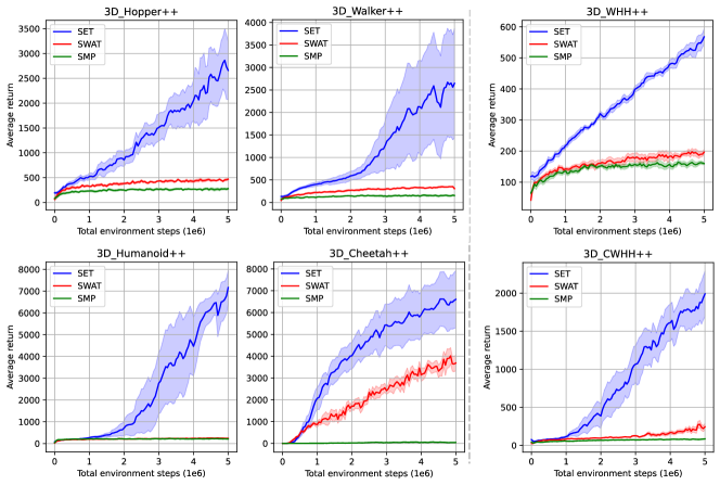
As shown in Figure 3, our Set outperforms all baselines by a large margin in all cases, indicating the remarkable superiority of taking into account the subequivariance upon Transformer. The baselines fail to achieve meaningful returns in most cases, which is possibly due to the large exploration space in our 3D-SGRL environments and they are prone to get trapped in local extreme points.
Zero-Shot Generalization
During test time, we assess the trained policy on a set of held-out agent morphologies. Table 2 records the results of both in-domain and cross-domain settings. The training and zero-shot testing variants are listed on Table 5. For example, Set is trained on 3D_Humanoid++ without 3d_humanoid_7_left_leg and 3d_humanoid_8_right_knee, while these two excluded environments are used for testing. Table 2 reports the average performance and the standard error over 3 seeds, where the return of each seed is calculated over 100 rollouts. Once again, we observe that Set yields better performance.
Evaluation on v2-variants
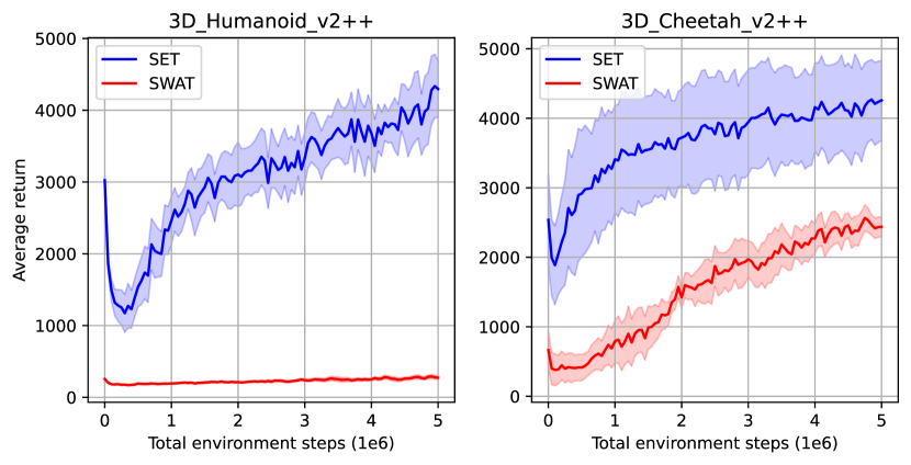
The v2-variants () are more challenging. We conduct two-stage training in this scenario. In the first stage, we train the policy under the multi-task setting where . The results and related demos are in Appendix F. In the second stage, we transfer the currently-trained policy to the setting on 3D_Cheetah++ and 3D_Humanoid++. It is seen from Figure 4 that Set is able to further improve the performance upon the first stage, while SWAT hardly receives meaningful performance gain especially on 3D_Humanoid++.
Single-task Learning
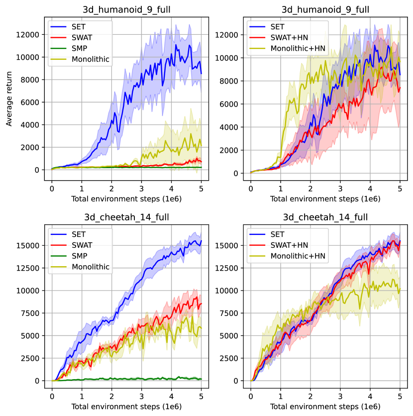
Apart from SMP and SWAT, we implement another baseline Monolithic for reference. Figure 5 displays the performance on 3d_humanoid_9_full and 3d_cheetah_14_full. In line with the observations in (Dong et al., 2022), the GNN-based method SMP is worse than the MLP-based model Monolithic; but different from the results in (Dong et al., 2022), SWAT still surpasses Monolithic on 3d_cheetah_14_full. We conjecture SWAT benefits from the application of Transformer that is expressive enough to characterize the variation of our 3d_cheetah_14_full environments. Our model Set takes advantage of both the expressive power of the Transformer-akin model and the rational constraint by subequivariance, hence it delivers much better performance than all other methods.
5.3 Comparison with Invariant Methods
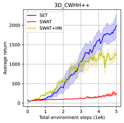
Invariant methods have been widely utilized in the 3D RL literature. For instance, in humanoid control, the presence of gravity allows for the normalization of state and action spaces in the heading (yaw) direction (e.g., a recent work (Won et al., 2022)). This heading normalization (HN) technique transforms the global coordinate frame into a local coordinate frame, enabling the input geometric information to be mapped to a rotation- and translation-invariant representation. We compare Set with the following invariant variants: 1. SWAT+HN: a state-of-the-art morphology-agnostic baseline that uses the heading normalization, and 2. Monolithic+HN: a standard TD3-based non-morphology-agnostic baseline that uses the heading normalization. As shown in Figure 5 and Figure 6, Set can only be considered on par with SWAT+HN, since heading normalization can achieve heading-equivariance by construction.
Indeed, there is a limitation of heading normalization in that it assumes a consistent definition of the “forward” direction across all agents. Without a consistent “forward” direction, the normalization scheme would need to be redefined for each individual agent, which could limit its transfer ability to different types of agents or environments. On the contrary, equivariant methods, such as the one proposed in our work, can be more generalizable as they do not rely on a specific normalization scheme and can adapt to different transformations in the environment. We design a simple experiment to verify the above statement by translating the “forward” direction of the agent via a certain bias angle during testing. Table 3 demonstrates the significant performance degradation caused by adding bias in the heading normalization. Moreover, we can support this point through zero-shot generalization experiments, where we evaluate the trained policies from multi-task on unseen zero-shot testing variants. Table 4 demonstrates that Set has stronger generalization ability compared to SWAT+HN. For more detailed discussions, please refer to Appendix D.
| Methods | 3d_humanoid_9_full | 3d_cheetah_14_full | ||
|---|---|---|---|---|
| Monolithic+HN | ||||
| SWAT+HN | ||||
| Set | ||||
| Environment | Set | SWAT+HN |
|---|---|---|
| cross-domain (3D_CWHH++) | ||
| 3d_walker_3 | ||
| 3d_walker_6 | ||
| 3d_humanoid_7 | ||
| 3d_humanoid_8 | ||
| 3d_cheetah_11 | ||
| 3d_cheetah_12 | ||
5.4 Ablation
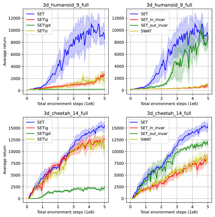
We ablate the following variants in Figure 7: 1. Setg: an -equivariant model, where gravity is removed from the external force and concatenated into the scalar input, ; 2. Setgd: an -equivariant model, where both and are considered as scalars: ; 3. Setz: an -equivariant model without Equation 5, by omitting the height ; 4. Set_in_invar: a non-equivariant model without all geometric vectors, instead taking them as the scalar input, ; 5. Set_out_invar: an -equivariant model by replacing the action output by the projection strategy in Equation 14 with an -invariant mapping .
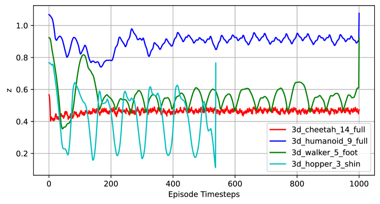
1. Setg and Setz, compared with Set, gain close performance on 3d_cheetah_14_full, but are much worse on 3d_humanoid_9_full. This is reasonable, as the agent 3d_cheetah_14_full has four legs and can locomote stably (see Figure 8). It is thus NOT so essential to consider the effect of gravity and the height to the ground on 3d_cheetah_14_full. As for 3d_humanoid_9_full with 2 legs, however, it is important to sense the direction of gravity and detect the height to avoid potential falling down, hence the correct modeling of gravity and the height are necessary for locomotion policy learning. 2. The performance of Setgd is poor in both cases, indicating that maintaining the direction information of the task guidance is indispensable. 3. Set_in_invar behaves much worse than Set, which verifies the importance to incorporate subequivariance into our model design. 4. Set_out_invar is worse than Set but already exceeds other variants. The equivariant output in Set contains rich orientation information, and it is more direct to obtain the output torque by projecting , than Set_out_invar which uses the invariant matrix to predict the action.
6 Discussion
In current machine learning research, equivariance and attention are both powerful ideas. To learn a shared graph-based policy in 3D-SGRL, we design Set, a novel transformer model that preserves geometric symmetry by construction. Experimental results strongly support the necessity of encoding symmetry into the policy network, which demonstrates its wide applicability in various 3D environments. We also compare the Monolithic MLP-based model using heading normalization for single-task training in Figure 5. It can be found that a simple MLP with heading normalization may outperform the benefits brought by equivariance and attention. Therefore, in comparison to traditional methods in single-task settings, we cannot guarantee that all humanoids and legged robots will experience considerable enhancement when using our equivariant methods. In this work, our main contribution is extending the 2D benchmark to 3D for morphology-agnostic RL, which mainly addresses challenges in multi-task learning with agents of inhomogeneous morphology where MLP may not be applicable. Although these are just initial steps, we believe that further exploration of this research direction will lead to valuable contributions to the research community.
Acknowledgements
This work is jointly funded by “New Generation Artificial Intelligence” Key Field Research and Development Plan of Guangdong Province (2021B0101410002), the National Science and Technology Major Project of the Ministry of Science and Technology of China (No.2018AAA0102900), the Sino-German Collaborative Research Project Crossmodal Learning (NSFC 62061136001/DFG TRR169), THU-Bosch JCML Center, the National Natural Science Foundation of China under Grant U22A2057, the National Natural Science Foundation of China (No.62006137), Beijing Outstanding Young Scientist Program (No.BJJWZYJH012019100020098), and Scientific Research Fund Project of Renmin University of China (Start-up Fund Project for New Teachers). We sincerely thank the reviewers for their comments that significantly improved our paper’s quality. Our heartfelt thanks go to Yu Luo, Tianying Ji, Chengliang Zhong, and Chao Yang for fruitful discussions. Finally, Runfa Chen expresses gratitude to his fiancée, Xia Zhong, for her unwavering love and support.
References
- Ba et al. (2016) Ba, J. L., Kiros, J. R., and Hinton, G. E. Layer normalization. arXiv preprint arXiv:1607.06450, 2016.
- Battaglia et al. (2018) Battaglia, P. W., Hamrick, J. B., Bapst, V., Sanchez-Gonzalez, A., Zambaldi, V., Malinowski, M., Tacchetti, A., Raposo, D., Santoro, A., Faulkner, R., et al. Relational inductive biases, deep learning, and graph networks. arXiv preprint arXiv:1806.01261, 2018.
- Chen et al. (2018) Chen, T., Murali, A., and Gupta, A. Hardware conditioned policies for multi-robot transfer learning. In Advances in Neural Information Processing Systems, volume 31, 2018.
- Cohen & Welling (2016) Cohen, T. S. and Welling, M. Group equivariant convolutional networks. In International Conference on Machine Learning, 2016.
- Cohen & Welling (2017) Cohen, T. S. and Welling, M. Steerable CNNs. In International Conference on Learning Representations, 2017.
- D’Eramo et al. (2020) D’Eramo, C., Tateo, D., Bonarini, A., Restelli, M., Peters, J., et al. Sharing knowledge in multi-task deep reinforcement learning. In International Conference on Learning Representations, 2020.
- Devin et al. (2017) Devin, C., Gupta, A., Darrell, T., Abbeel, P., and Levine, S. Learning modular neural network policies for multi-task and multi-robot transfer. In 2017 IEEE International Conference on Robotics and Automation, pp. 2169–2176. IEEE, 2017.
- Dong et al. (2022) Dong, H., Wang, T., Liu, J., and Zhang, C. Low-rank modular reinforcement learning via muscle synergy. In Advances in Neural Information Processing Systems, 2022.
- Fuchs et al. (2020) Fuchs, F., Worrall, D., Fischer, V., and Welling, M. Se(3)-transformers: 3d roto-translation equivariant attention networks. In Advances in Neural Information Processing Systems, volume 33, pp. 1970–1981. Curran Associates, Inc., 2020.
- Fujimoto et al. (2018) Fujimoto, S., Hoof, H., and Meger, D. Addressing function approximation error in actor-critic methods. In International Conference on Machine Learning, pp. 1587–1596. PMLR, 2018.
- Furuta et al. (2023) Furuta, H., Iwasawa, Y., Matsuo, Y., and Gu, S. S. A system for morphology-task generalization via unified representation and behavior distillation. In International Conference on Learning Representations, 2023.
- Gupta et al. (2022) Gupta, A., Fan, L., Ganguli, S., and Fei-Fei, L. Metamorph: Learning universal controllers with transformers. In International Conference on Learning Representations, 2022.
- Han et al. (2022a) Han, J., Huang, W., Ma, H., Li, J., Tenenbaum, J. B., and Gan, C. Learning physical dynamics with subequivariant graph neural networks. In Advances in Neural Information Processing Systems, volume 35, pp. 26256–26268, 2022a.
- Han et al. (2022b) Han, J., Rong, Y., Xu, T., and Huang, W. Geometrically equivariant graph neural networks: A survey. arXiv preprint arXiv:2202.07230, 2022b.
- Hong et al. (2021) Hong, S., Yoon, D., and Kim, K.-E. Structure-aware transformer policy for inhomogeneous multi-task reinforcement learning. In International Conference on Learning Representations, 2021.
- Hsu et al. (2022) Hsu, C., Verkuil, R., Liu, J., Lin, Z., Hie, B., Sercu, T., Lerer, A., and Rives, A. Learning inverse folding from millions of predicted structures. In International Conference on Machine Learning, pp. 8946–8970. PMLR, 2022.
- Huang et al. (2020) Huang, W., Mordatch, I., and Pathak, D. One policy to control them all: Shared modular policies for agent-agnostic control. In International Conference on Machine Learning, pp. 4455–4464. PMLR, 2020.
- Huang et al. (2022) Huang, W., Han, J., Rong, Y., Xu, T., Sun, F., and Huang, J. Equivariant graph mechanics networks with constraints. In International Conference on Learning Representations, 2022.
- Jørgensen & Bhowmik (2022) Jørgensen, P. B. and Bhowmik, A. Equivariant graph neural networks for fast electron density estimation of molecules, liquids, and solids. npj Computational Materials, 8(1):183, 2022.
- Joshi et al. (2022) Joshi, C. K., Bodnar, C., Mathis, S. V., Cohen, T., and Liò, P. On the expressive power of geometric graph neural networks. In NeurIPS 2022 Workshop on Symmetry and Geometry in Neural Representations, 2022.
- Kurin et al. (2020) Kurin, V., Igl, M., Rocktäschel, T., Boehmer, W., and Whiteson, S. My body is a cage: the role of morphology in graph-based incompatible control. In International Conference on Learning Representations, 2020.
- Lillicrap et al. (2016) Lillicrap, T. P., Hunt, J. J., Pritzel, A., Heess, N., Erez, T., Tassa, Y., Silver, D., and Wierstra, D. Continuous control with deep reinforcement learning. In International Conference on Learning Representations, 2016.
- Mnih et al. (2015) Mnih, V., Kavukcuoglu, K., Silver, D., Rusu, A. A., Veness, J., Bellemare, M. G., Graves, A., Riedmiller, M., Fidjeland, A. K., Ostrovski, G., et al. Human-level control through deep reinforcement learning. Nature, 518(7540):529–533, 2015.
- Mnih et al. (2016) Mnih, V., Badia, A. P., Mirza, M., Graves, A., Lillicrap, T., Harley, T., Silver, D., and Kavukcuoglu, K. Asynchronous methods for deep reinforcement learning. In International Conference on Machine Learning, pp. 1928–1937. PMLR, 2016.
- Pathak et al. (2019) Pathak, D., Lu, C., Darrell, T., Isola, P., and Efros, A. A. Learning to control self-assembling morphologies: a study of generalization via modularity. In Advances in Neural Information Processing Systems, volume 32, 2019.
- Satorras et al. (2021) Satorras, V. G., Hoogeboom, E., and Welling, M. E (n) equivariant graph neural networks. In International Conference on Machine Learning, pp. 9323–9332. PMLR, 2021.
- Schulman et al. (2017) Schulman, J., Wolski, F., Dhariwal, P., Radford, A., and Klimov, O. Proximal policy optimization algorithms. arXiv preprint arXiv:1707.06347, 2017.
- Schütt et al. (2021) Schütt, K., Unke, O., and Gastegger, M. Equivariant message passing for the prediction of tensorial properties and molecular spectra. In International Conference on Machine Learning, pp. 9377–9388. PMLR, 2021.
- Silver et al. (2016) Silver, D., Huang, A., Maddison, C. J., Guez, A., Sifre, L., Van Den Driessche, G., Schrittwieser, J., Antonoglou, I., Panneershelvam, V., Lanctot, M., et al. Mastering the game of go with deep neural networks and tree search. Nature, 529(7587):484–489, 2016.
- Tassa et al. (2012) Tassa, Y., Erez, T., and Todorov, E. Synthesis and stabilization of complex behaviors through online trajectory optimization. In 2012 IEEE/RSJ International Conference on Intelligent Robots and Systems, pp. 4906–4913. IEEE, 2012.
- Thomas et al. (2018) Thomas, N., Smidt, T., Kearnes, S., Yang, L., Li, L., Kohlhoff, K., and Riley, P. Tensor field networks: Rotation-and translation-equivariant neural networks for 3d point clouds. arXiv preprint arXiv:1802.08219, 2018.
- Todorov et al. (2012) Todorov, E., Erez, T., and Tassa, Y. Mujoco: A physics engine for model-based control. In 2012 IEEE/RSJ International Conference on Intelligent Robots and Systems, pp. 5026–5033. IEEE, 2012.
- Trabucco et al. (2022) Trabucco, B., Phielipp, M., and Berseth, G. Anymorph: Learning transferable polices by inferring agent morphology. In International Conference on Machine Learning, pp. 21677–21691. PMLR, 2022.
- van der Pol et al. (2020) van der Pol, E., Worrall, D., van Hoof, H., Oliehoek, F., and Welling, M. Mdp homomorphic networks: Group symmetries in reinforcement learning. In Advances in Neural Information Processing Systems, volume 33, pp. 4199–4210, 2020.
- Vaswani et al. (2017) Vaswani, A., Shazeer, N., Parmar, N., Uszkoreit, J., Jones, L., Gomez, A. N., Kaiser, Ł., and Polosukhin, I. Attention is all you need. In Advances in Neural Information Processing Systems, volume 30, 2017.
- Villar et al. (2021) Villar, S., Hogg, D. W., Storey-Fisher, K., Yao, W., and Blum-Smith, B. Scalars are universal: Equivariant machine learning, structured like classical physics. In Advances in Neural Information Processing Systems, volume 34, pp. 28848–28863, 2021.
- Wang et al. (2018) Wang, T., Liao, R., Ba, J., and Fidler, S. Nervenet: Learning structured policy with graph neural networks. In International conference on learning representations, 2018.
- Wawrzynski (2007) Wawrzynski, P. Learning to control a 6-degree-of-freedom walking robot. In EUROCON 2007-The International Conference on” Computer as a Tool”, pp. 698–705. IEEE, 2007.
- Wawrzyński (2009) Wawrzyński, P. A cat-like robot real-time learning to run. In International Conference on Adaptive and Natural Computing Algorithms, pp. 380–390. Springer, 2009.
- Won et al. (2022) Won, J., Gopinath, D., and Hodgins, J. Physics-based character controllers using conditional vaes. ACM Transactions on Graphics (TOG), 41(4):1–12, 2022.
- Worrall et al. (2017) Worrall, D. E., Garbin, S. J., Turmukhambetov, D., and Brostow, G. J. Harmonic networks: Deep translation and rotation equivariance. In Proceedings of the IEEE Conference on Computer Vision and Pattern Recognition, pp. 5028–5037, 2017.
Appendix A Proofs
In this section, we theoretically prove that our proposed SubEquivariant Transformer (Set), and the final output action and critic Q-function value preserve the symmetry as desired. We start by verifying our design in Set.
Theorem A.1.
Let , where is one layer of our Set specified from Equation 7 to Equation 12. Let . Then, we have , indicating is -equivariant.
Proof.
In the first place, we have . For the message , we have,
| (16) | ||||
| (17) | ||||
| (18) | ||||
| (19) | ||||
| (20) |
From Equation 18 to Equation 19 we use the fact and , by the definition of the group . With the -invariant message , it is then immediately illustrated that the query , key , value message , and the attention coefficient are all -invariant, and value message is -equivariant. Finally, we have,
| (21) | ||||
| (22) | ||||
| (23) | ||||
| (24) |
and similarly,
| (25) |
By going through all nodes the proof is completed. ∎
By iteratively applying Theorem A.1 for layers, we readily obtain the -equivariance of the entire Set.
As for the actor and critic, we additionally have the following corollary.
Corollary A.2.
Let be the output action and the critic of 3D-SGRL with as input. Let be the action and critic with as input, . Then, , indicating the output action and critic preserve -invariance.
Proof.
By Theorem A.1, we have , and . Therefore, . Hence,
| (26) | ||||
| (27) | ||||
| (28) |
where Equation 26 to Equation 27, again, leverages the fact that , given the definition of . Finally,
| (29) | ||||
| (30) |
and meanwhile,
| (31) |
since concatenating the -invariant into the input does not affect the -invariance of the message .
∎
Appendix B Related Works
Morphology-Agnostic RL
In recent years, we have seen the emergence and development of multi-task RL with the inhomogeneous morphology setting, where the state and action spaces are different across tasks (Devin et al., 2017; Chen et al., 2018; D’Eramo et al., 2020). The morphology-agnostic approach, which learns policies for each joint using multiple message passing schemes, decentralizes the control of multi-joint robots. In order to deal with the inhomogeneous setting, NerveNet (Wang et al., 2018), DGN (Pathak et al., 2019) and SMP (Huang et al., 2020) represent the morphology of the agent as a graph and deploy GNNs as the policy network. Amorpheus (Kurin et al., 2020), SWAT (Hong et al., 2021) and Solar (Dong et al., 2022) utilize the self-attention mechanism instead of GNNs for direct communication. In morphology-agnostic RL, both of their investigations demonstrate that the graph-based policy has significant advantages over a monolithic policy. Our work is based on SWAT and introduces a set of new benchmarks that relax the over-simplified state and action space of existing works to a much more challenging scenario with immersive search space.
Geometrically Equivariant Models
Prominently, there are certain symmetries in the physical world and there have been a number of studies about group equivariant models (Cohen & Welling, 2016, 2017; Worrall et al., 2017). In recent years, a field of research known as geometrically equivariant graph neural networks (Han et al., 2022b), leverages symmetry as an inductive bias in learning. These models are designed such that their outputs will rotate/translate/reflect in the same way as the inputs, hence retaining the symmetry. Several methods are used to achieve this goal, such as using irreducible representation to solve group convolution (Thomas et al., 2018; Fuchs et al., 2020) or utilizing invariant scalarization (Villar et al., 2021) like taking the inner product (Satorras et al., 2021; Huang et al., 2022; Han et al., 2022a). Along with GMN’s (Huang et al., 2022) and SGNN’s (Han et al., 2022a) approaches to scalarization, our method is a member of this family. In a Markov decision process (MDP) with symmetries (van der Pol et al., 2020), there are symmetries in the state-action space where policies can thus be optimized in the simpler abstract MDP. van der Pol et al. (2020) attempts to learn equivariant policy and invariant value networks in 2D toy environments. Our work focuses on the realization of this motivation in more complex 3D physics simulation environments.
Appendix C More Experimental Details
C.1 Environments and Agents
We choose the following environments from morphology-agnostic RL benchmark (Huang et al., 2020) to evaluate our methods: Hopper++, Walker++, Humanoid++, Cheetah++. To facilitate the study of subequivariant graph reinforcement learning across these agents, we modify the 2D-Planar agents and extend them into 3D agents. Specifically, we modify the joint of torso from the combination of “slide-slide-hinge” type to “free” type. Normally, each joint of the agent in the 2D-Planar environment has only one hinge-type actuator to make it rotate around -axis. In order to make the agent more flexible to explore and optimize the learning process, we expand its action space including increasing the number of hinge-type actuators from 1 to 3, thus the DoF of each joint is also enlarged to 3. The two newly-added actuators enable the joint to basically rotate around -axis and -axis, respectively.
3D Hopper: The rotation range of the joint’s two newly-added actuators is limited to .
3D Walker: The legs of 3D Walker is designed with reference to the legs of standard 3D Humanoid (Tassa et al., 2012). The rotation range of each joint is limited to new intervals. The rotation range of the joints in left and right leg are the same, we only show the intervals of a joint of the left leg:
| the joint of thigh: | |||
| the joint of shin: | |||
| the joint of foot: |
3D Humanoid: We refer to the standard 3D Humanoid (Tassa et al., 2012) and expand the number of actuators. The rotation range of newly-added joint actuators are limited to .
3D Cheetah: The standard half-cheetah (Wawrzynski, 2007; Wawrzyński, 2009) is specially designed as a planar model of a walking animal, which would not fall over in 2D-Planar environments, so there is no interruption in each episode. But in 3D-SGRL environments, the half-cheetah very easy to falls over and this will interrupt its learning process, making it more difficult for effective locomotion. So we modify the model of a half-cheetah into a full-cheetah, and its torso, four legs and tail are made of 14 limbs. 3D Cheetah is about 1.1 meters long, 0.6 meters high and weighs 55kg. We limit the “strengths” of its joints within the range from 30 to 120Nm. So it is designed as a 3D model of a large and agile cat with many joints yet smaller strength, making it more stable and less easy to fall over in 3D-SGRL environments while retaining a strong locomotion ability. As a result, the full-cheetah is more adaptable to 3D-SGRL environments. The rotation range of joints is limited to new intervals. The rotation range of the tail is . The rotation range of the left limb and the right limb are the same, we only show the intervals of those left:
| the joint of back thigh: | |||
| the joint of back shin: | |||
| the joint of back foot: | |||
| the joint of front thigh: | |||
| the joint of front shin: | |||
| the joint of front foot: |
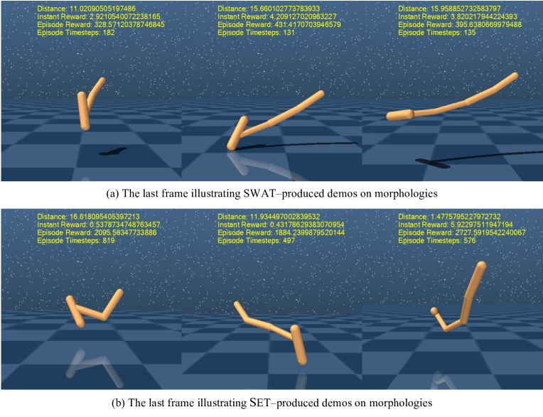
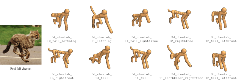
To systematically investigate the proposed method applied to multi-task training, we construct several variants from the agents we mentioned above, as shown in Table 5. The morphologies of ten variants of 3D Cheetah are different from that of the 2D-Planar, as is shown in Figure 9.
| Environment | Training | Zero-shot testing |
| 3D_Hopper++ | ||
| 3d_hopper_3_shin | ||
| 3d_hopper_4_lower_shin | ||
| 3d_hopper_5_full | ||
| 3D_Walker++ | ||
| 3d_walker_2_right_leg_left_knee | 3d_walker_3_left_knee_right_knee | |
| 3d_walker_3_left_leg_right_foot | 3d_walker_6_right_foot | |
| 3d_walker_4_right_knee_left_foot | ||
| 3d_walker_5_foot | ||
| 3d_walker_5_left_knee | ||
| 3d_walker_7_full | ||
| 3D_Humanoid++ | ||
| 3d_humanoid_7_left_arm | 3d_humanoid_7_left_leg | |
| 3d_humanoid_7_lower_arms | 3d_humanoid_8_right_knee | |
| 3d_humanoid_7_right_arm | ||
| 3d_humanoid_7_right_leg | ||
| 3d_humanoid_8_left_knee | ||
| 3d_humanoid_9_full | ||
| 3D_Cheetah++ | ||
| 3d_cheetah_10_tail_leftbleg | 3d_cheetah_11_leftbkneen_rightffoot | |
| 3d_cheetah_11_leftfleg | 3d_cheetah_12_tail_leftffoot | |
| 3d_cheetah_11_tail_rightfknee | ||
| 3d_cheetah_12_rightbknee | ||
| 3d_cheetah_12_tail_leftbfoot | ||
| 3d_cheetah_13_rightffoot | ||
| 3d_cheetah_13_tail | ||
| 3d_cheetah_14_full | ||
| 3D_Walker-3D_Humanoid-3D_Hopper++(3D_WHH++) | ||
| Union of 3D_Walker++, 3D_Humanoid++ and 3D_Hopper++ | ||
| 3D_Cheetah-3D_Walker-3D_Humanoid-3D_Hopper++(3D_CWHH++) | ||
| Union of 3D_Cheetah++, 3D_Walker++, 3D_Humanoid++ and 3D_Hopper++ | ||
C.2 Baselines
This part illustrates the implementations of these baselines.
SMP
Huang et al. (2020) employs GNNs as policy networks and uses both bottom-up and top-down message passing schemes through the links between joints for coordinating. We use the implementation of SMP in the SWAT codebase, which is the same as the original implementation of SMP provided by Huang et al. (2020).
SWAT
All of the GNN-like works show that morphology-agnostic policies are more advantageous than the monolithic policy in tasks aiming at tackling different morphologies. However, Kurin et al. (2020) validate a hypothesis that the benefit extracted from morphological structures by GNNs can be offset by their negative effect on message passing. They further propose a transformer-based method, Amorpheus, which relies on mechanisms for self-attention as a way of message transmission. Hong et al. (2021) make use of morphological traits via structural embeddings, enabling direct communication and capitalizing on the structural bias. We use the original implementation of SWAT released by Hong et al. (2021). For a fair comparison, Set uses the same hyperparameters as SWAT (Table 6).
Monolithic
We choose TD3 as the standard monolithic RL baseline. The actor and critic of TD3 are implemented by fully-connected neural networks.
C.3 Implementation details
For the scalar features , in addition to retaining the original rotation angle of joint, we also undergo the following processing: the rotation angle and range of joint are represented as three scalar numbers normalized to , where is the joint position at time , and is the allowed joint range. The type of limb is a 4-dimensional one-hot vector representing “torso”, “thigh”, “shin”, “foot” and “other” respectively. Besides, note that the torso limb has no joint actuator in any of these environments, so we ignore its predicted torque values. We implement Set based on SWAT codebase (Hong et al., 2021), which is built on Official PyTorch Tutorial. SWAT also shares the codebase with SMP (Huang et al., 2020) and Amorpheus (Kurin et al., 2020). Table 6 provides the hyperparameters needed to replicate our experiments. Our codes are available on https://github.com/alpc91/SGRL.
| Hyperparameter | Value |
| Learning rate | 0.0001 |
| Gradient clipping | 0.1 |
| Normalization | LayerNorm |
| Total attention layers | 3 |
| Attention heads | 2 |
| Attention embedding size | 128 |
| Attention hidden size | 256 |
| Matrix embedding size | 3232 |
| Matrix hidden size | 512 |
| Encoder output size | 128 |
| Mini-batch size | 100 |
| Maximum Replay buffer size | 10M |
Appendix D More Discussion about Invariant Methods
Specifically, by choosing the “forward” direction, we can achieve heading-equivariance with heading normalization. In essence, the lack of a predetermined “forward” direction that is consistent across all agents prevents us from transferring experiences between different agents. For example, if we create a duplicate of one agent and redefine the “forward” direction, heading normalization will no longer be applicable. In particular, let’s consider two agents that have very similar morphology, with the only difference being that their torso orientations are opposite and both encourage movement along the torso orientation. If the torso orientation is selected as the “forward” direction, the normalization applied to these two agents will vary significantly. As a result, the policy learned by one agent will not generalize to the other agent, unless the other agent’s movement mode is to move in the opposite orientation of the torso. Therefore, generalization performance is affected by the choice of the “forward” direction and the agent’s movement mode.
Besides, there is extensive experimental evidence (Hsu et al., 2022; Jørgensen & Bhowmik, 2022; Schütt et al., 2021; Joshi et al., 2022) indicating that equivariant methods that preserve equivariance at each layer outperform those invariant methods that solely apply transformations at the input layer to obtain invariant features and then use an invariant network. Our framework, falling into the equivariant family, enables the propagation of directional information through message passing steps, allowing the extraction of rich geometric information such as angular messages. In contrast, the invariant methods may result in the loss of higher-order correlations between nodes, which are crucial for modeling the geometric relationships between them.
Appendix E More Ablation on Equivariance
In addition, we conduct another experiment by fixing the initial orientation as 0° when training, but allowing arbitrary angles when testing. As shown in Table 7, Set generalizes well to all cases. On the contrary, SWAT only obtains desirable performance when the testing angle is fixed to 0° which is the same as that during the training process, and its performance drops rapidly in other cases, especially at 180°. The experiments here justify the efficacy of involving orthogonality equivariance.
| Methods | 500k training steps | 1M training steps | ||||||||
|---|---|---|---|---|---|---|---|---|---|---|
| random | random | |||||||||
| SWAT | ||||||||||
| Set | ||||||||||
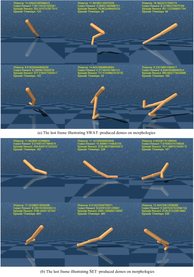
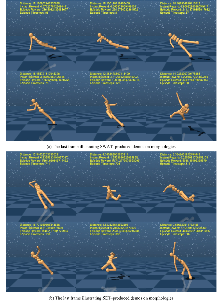
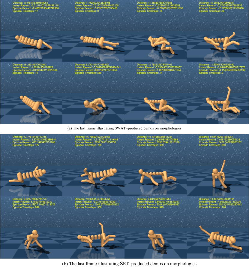
Appendix F The Evaluation on v2-variants
The v2-variants () are more challenging. We train the policy in the multi-task setting where , then we do the test in v2-variants. The results and related demos are shown in Figure 10, Figure 11, Figure 12 and Figure 13. While SWAT fails to perform well, Set has obvious advantages. With more episode timesteps, Set locomotes closer to the destination (a shorter distance) and gets more episode rewards.
