Representation and Simulation of Multivariate Dickman Distributions and Vervaat Perpetuities

Abstract

A multivariate extension of the Dickman distribution was recently introduced, but very few properties have been studied. We discuss several properties with an emphasis on simulation. Further, we introduce and study a multivariate extension of the more general class of Vervaat perpetuities and derive a number of properties and representations. Most of our results are presented in the even more general context of so-called $\alpha$-times self-decomposable distributions.

Keywords: Multivariate Dickman distribution; Multivariate Vervaat perpetuities; Self-decomposable distributions; Simulation

1 Introduction

The Dickman distribution arises in many applications, including in the study of random graphs, small jumps of Lévy processes, and Hoare’s quickselect algorithm. It is closely related to the Dickman function, which is important in the study of prime numbers. For details and many applications see the recent surveys [20], [19], and [14]. The class of Vervaat perpetuities is closely related to the Dickman distribution and has applications in a variety of areas including economics, actuarial science, and astrophysics, see the references in [8]. Recently, there has been much interest in the simulation of Dickman random variables and Vervaat perpetuities. This was studied in a series of papers, including [9], [10], [11], [4], [5], and [8]. A multivariate extension of the Dickman distribution was recently introduced in [1], where it arose in the context of a limit theorem related to certain point processes. However, very few properties of the multivariate Dickman distribution have been studied and, from what we have seen, a multivariate extension of Vervaat perpetuities has not been introduced.

In this paper, we introduce a multivariate extension of the class of Vervaat perpetuities, which includes the multivariate Dickman distribution as a special case. We show that these distributions are infinitely divisible and, more specifically, that they coincide with the class of self-decomposable distributions with finite background driving Lévy measures, no Gaussian part, and no drift. We have not seen this relationship mentioned previously even in the univariate case, although connections between the class of self-decomposable distribution and more general classes of perpetuities are known, see [15]. In the interest of generality, our theoretical results are derived in the more general context of $\alpha$-times self-decomposable distributions. For these we derive three representations: as stochastic integrals, as shot noise, and as limits of certain triangular arrays. The latter two can be used for simulation. Further, for the multivariate Dickman distribution, we propose a third simulation method, which is based on a discretization of the spectral measure and is similar to the approach used in [30] for simulating multivariate tempered stable distributions.

The need for simulation methods is motivated by the fact that the Dickman distribution can be used to model the small jumps of large classes of Lévy processes. In the univariate case this was shown in [7]; we will extend it to the multivariate case in a forthcoming work. The simulation of large jumps tends to be easier as they follow a compound Poisson distribution. Combining the two allows for the simulation of a wide variety of Lévy processes, which can then be used for many applications. Our motivation comes from finance, where Monte Carlo methods based on Lévy processes are often used for option pricing, see, e.g., [6]. In particular, the ability to simulate multivariate Lévy processes allows for the pricing of multi-asset, e.g., rainbow or basket options.

The rest of this paper is organized as follows. In Section 2 we recall basic facts about $\alpha$-times self-decomposable distributions and give our main theoretical results. In Section 3, we formally introduce the multivariate Dickman distribution and multivariate Vervaat perpetuities. In Section 4 we discuss three approximate simulation methods for the multivariate Dickman distribution with an emphasis on the bivariate case. A small-scale simulation study is conducted in Section 5. Proof are postponed to Section 6.

Before proceeding, we introduce some notation. We write $\mathbb{R}^{d}$ to denote the space of $d$-dimensional column vectors of real numbers, $\mathbb{S}^{d-1}=\{x\in\mathbb{R}^{d}:|x|=1\}$ to denote the unit sphere in $\mathbb{R}^{d}$, and $\mathfrak{B}(\mathbb{R}^{d})$ and $\mathfrak{B}(\mathbb{S}^{d-1})$ to denote the classes of Borel sets on $\mathbb{R}^{d}$ and $\mathbb{S}^{d-1}$, respectively. For a distribution $\mu$ on $\mathbb{R}^{d}$, we write $\hat{\mu}$ to denote its characteristic function, $X\sim\mu$ to denote that $X$ is a random variable with distribution $\mu$, and $X_{1},X_{2},\dots\stackrel{{\scriptstyle\mathrm{iid}}}{{\sim}}\mu$ to denote that $X_{1},X_{2},\dots$ are independent and identically distributed (iid) random variables with distribution $\mu$. We write $U(0,1)$ to denote the uniform distribution on $(0,1)$, $\mathrm{Exp}(\lambda)$ to denote the exponential distribution with rate $\lambda$, $\delta_{a}$ to denote a point-mass at $a$, and $1_{A}$ to denote the indicator function on event $A$. We write $\Gamma$ to denote the gamma function, $\lfloor\cdot\rfloor$ to denote the floor function, and $\vee$ and $\wedge$ to denote the maximum and minimum, respectively. We write $\stackrel{{\scriptstyle d}}{{=}}$, $\stackrel{{\scriptstyle d}}{{\rightarrow}}$, and $\stackrel{{\scriptstyle w}}{{\rightarrow}}$ to denote equality in distribution, convergence in distribution, and weak convergence, respectively. For two sequences of real numbers $\{a_{n}\}$ and $\{b_{n}\}$, we write $a_{n}\sim b_{n}$ to denote $a_{n}/b_{n}\to 1$ as $n\to\infty$.

2 $\alpha$-times self-decomposable distributions and main results

We begin by recalling that the characteristic function of an infinitely divisible distribution $\mu$ on $\mathbb{R}^{d}$ can be written in the form $\hat{\mu}(z)=\exp\{C_{\mu}(z)\}$, where

$$C_{\mu}(z)=-\langle z,Az\rangle+i\left\langle b,z\right\rangle+\int_{\mathbb{R}^{d}}\left(e^{i\left\langle z,x\right\rangle}-1-\left\langle z,x\right\rangle 1_{[|x|\leq 1]}\right)M(\mathrm{d}x),\ \ \ z\in\mathbb{R}^{d},$$

$A$ is a $d\times d$-dimensional covariance matrix called the Gaussian part, $b\in\mathbb{R}^{d}$ is the shift, and $M$ is the Lévy measure, which is a Borel measure on $\mathbb{R}^{d}$ satisfying

$$M(\{0\})=0\text{ and }\int_{\mathbb{R}^{d}}(|x|^{2}\wedge 1)M(\mathrm{d}x)<\infty.$$

The parameters $A$, $M$, and $b$ uniquely determine this distribution and we write $\mu=\mathrm{ID}(A,M,b)$. We call $C_{\mu}$ the cumulant generating function (cgf) of $\mu$. Associated with every infinitely divisible distribution $\mu$ is a Lévy process $\{X_{t}:t\geq 0\}$, where $X_{1}\sim\mu$. This process has finite variation if and only if $A=0$ and $M$ satisfies the additional assumption

$$\int_{\mathbb{R}^{d}}(|x|\wedge 1)M(\mathrm{d}x)<\infty.$$ (1)

Through a slight abuse of terminology, we also say that the associated distribution $\mu$ has finite variation. In this case, the cgf can be written in the form

$$C_{\mu}(z)=i\left\langle\gamma,z\right\rangle+\int_{\mathbb{R}^{d}}\left(e^{i\left\langle z,x\right\rangle}-1\right)M(\mathrm{d}x),\ \ \ z\in\mathbb{R}^{d},$$ (2)

where $\gamma=b-\int_{|x|\leq 1}xM(\mathrm{d}x)\in\mathbb{R}^{d}$ is the drift and we write $\mu=\mathrm{ID}_{0}(M,\gamma)$.

A distribution $\mu$ is said to be self-decomposable if for any $c\in(0,1)$ there exists a probability measure $\rho_{c}$ with

$$\hat{\mu}(z)=\hat{\mu}(cz)\hat{\rho}_{c}(z),\ \ z\in\mathbb{R}^{d}.$$ (3)

Equivalently, if $X\sim\mu$ and $Y_{c}\sim\rho_{c}$, then $X\stackrel{{\scriptstyle d}}{{=}}cX+Y_{c}$, where $X$ and $Y_{c}$ are independent on the right side. We denote the class of self-decomposable distributions by $L_{1}$. These distributions are important in the study of stationary $\mathrm{AR}(1)$ processes and the limits of sums of independent random variables. Next, for $\alpha\in\{2,3,\dots\}$ we define the classes $L_{\alpha}$ recursively, as follows. A distribution $\mu\in L_{\alpha}$ if for every $c\in(0,1)$ there exists a $\rho_{c}\in L_{\alpha-1}$ such that (3) holds. There is substantial literature on the study of these classes, see, e.g., the monograph [22] and the references therein. The distributions in $L_{\alpha}$ are sometimes called $\alpha$-times self-decomposable. These should not be confused with the so-called $\alpha$-self-decomposable distributions, studied in, e.g., [17] and the references therein.

It is well-known that every $\mu\in L_{\alpha}$ is infinitely divisible. In fact, $\mu\in L_{\alpha}$ if and only if $\mu=\mathrm{ID}(A,M,b)$ with $M=M_{\alpha}$, where

$$M_{\alpha}(B)=\int_{\mathbb{R}^{d}}\int_{0}^{1}1_{B}(yr)(-\log r)^{\alpha-1}r^{-1}\mathrm{d}r\nu(\mathrm{d}y),\ \ \ B\in\mathfrak{B}(\mathbb{R}^{d}),$$ (4)

for some Borel measure $\nu$ satisfying

$$\nu(\{0\})=0\ \mbox{ and }\ \int_{|x|\leq 2}|x|^{2}\nu(\mathrm{d}x)+\int_{|x|>2}\left(\log|x|\right)^{\alpha}\nu(\mathrm{d}x)<\infty.$$ (5)

Clearly, $M_{\alpha}$ can be a Lévy measure even if $\alpha$ is not an integer. In fact, $M_{\alpha}$ is a Lévy measure for any $\alpha>0$ so long as (5) holds. The study of this extension to non-integer $\alpha$ was initiated in [28], see also [26] and the references therein. This leads to the following.

Definition 1.

Fix $\alpha\in(0,\infty)$. We write $L_{\alpha}$ to denote the class of all infinitely divisible distributions $\mathrm{ID}(A,M,b)$ where $M=M_{\alpha}$ is of the form (4) for some Borel measure $\nu$ on $\mathbb{R}^{d}$ satisfying (5). We refer to $L_{\alpha}$ as the class of $\alpha$-times self-decomposable distributions. The measure $\nu$ is called the background driving Lévy measure (BDLM).

The name BDLM is motivated by the role that this measure plays in the context of OU-processes, see [22]. We now give a result that relates certain moment properties of $M_{\alpha}$ to those of the BDLM $\nu$.

Lemma 1.

Fix $\alpha\in(0,\infty)$ and let $M_{\alpha}$ be as in (4), where $\nu$ is a Borel measure on $\mathbb{R}^{d}$ satisfying (5). In this case we can equivalently write

$$M_{\alpha}(B) = \int_{\mathbb{R}^{d}}\int_{0}^{\infty}1_{B}(ye^{-r})r^{\alpha-1}\mathrm{d}r\nu(\mathrm{d}y)$$ (6)

$$= \theta^{-1}\int_{\mathbb{R}^{d}}\int_{0}^{\infty}1_{B}(ye^{-(\alpha r/\theta)^{1/\alpha}})\mathrm{d}r\nu(\mathrm{d}y),\ \ \ B\in\mathfrak{B}(\mathbb{R}^{d})$$

for any $\theta>0$. Further, $M_{\alpha}(\mathbb{R}^{d})=\infty$ for any $\nu\neq 0$ and for any $p>0$, we have

$$\int_{|x|\leq 1}|x|^{p}M_{\alpha}(\mathrm{d}x)<\infty\mbox{ if and only if }\int_{|x|\leq 1}|x|^{p}\nu(\mathrm{d}x)<\infty$$

and

$$\int_{|x|>1}|x|^{p}M_{\alpha}(\mathrm{d}x)<\infty\mbox{ if and only if }\int_{|x|>1}|x|^{p}\nu(\mathrm{d}x)<\infty.$$

Combining the lemma with Proposition 25.4 in [24] shows that for $X\sim\mu\in L_{\alpha}$ with BDLM $\nu$ and any $p>0$ we have

$$\mathrm{E}|X|^{p}<\infty\mbox{ if and only if }\int_{|x|>1}|x|^{p}\nu(\mathrm{d}x)<\infty.$$

In the context of multivariate Vervaat perpetuities, we are only interested in distributions with no Gaussian part and a finite BDLM. In this case, Lemma 1 imples that $M_{\alpha}$ will satisfy (1), which leads to the following.

Definition 2.

Fix $\alpha\in(0,\infty)$. We write $L^{*}_{\alpha}$ to denote the class of all infinitely divisible distribution $\mu=\mathrm{ID}_{0}(M,\gamma)$ where $M=M_{\alpha}$ is of the form (4) for some finite Borel measure $\nu$ on $\mathbb{R}^{d}$ satisfying (5). In this case, we write $\mu=L^{*}_{\alpha}(\nu,\gamma)$.

From (2) and (4) it follows that the cgf of $L^{*}_{\alpha}(\nu,\gamma)$ is given by

$$i\langle\gamma,z\rangle+\int_{\mathbb{R}^{d}}\int_{0}^{1}\left(e^{ir\left\langle z,y\right\rangle}-1\right)(-\log r)^{\alpha-1}r^{-1}\mathrm{d}r\nu(\mathrm{d}y),\ \ \ z\in\mathbb{R}^{d}.$$

Taking partial derivatives shows that, when they exist, the mean vector and covariance matrix of $X\sim L^{*}_{\alpha}(\nu,\gamma)$ are given by

$$\mathrm{E}[X]=\gamma+\Gamma(\alpha)\int_{\mathbb{R}^{d}}y\nu(\mathrm{d}y)\mbox{ and }\mathrm{cov}(X)=\frac{\Gamma(\alpha)}{2^{\alpha}}\int_{\mathbb{R}^{d}}yy^{T}\nu(\mathrm{d}y).$$ (7)

Next, we give three representations of the distributions in $L^{*}_{\alpha}$. The first as a stochastic integral, the second as shot noise, and the third as the limit of a triangular array. The first result is essentially contained in [26], but, for completeness and due to a difference in presentation, a self-contained proof is given in Section 6.

Theorem 1.

Let $X\sim L^{*}_{\alpha}(\nu,\gamma)$ and fix $\theta>0$. If $\{Y_{t}:t\geq 0\}$ is a Lévy process with $Y_{1}\sim\mathrm{ID}_{0}(\nu^{\prime},\gamma^{\prime})$, where $\nu^{\prime}=\nu/\theta$ and $\gamma^{\prime}=\gamma/(\theta\Gamma(\alpha))$, then

$$X\stackrel{{\scriptstyle d}}{{=}}\int_{0}^{\infty}e^{-\left(\frac{\alpha s}{\theta}\right)^{1/\alpha}}\mathrm{d}Y_{s},$$

where the stochastic integral is absolutely definable in the sense of [25].

Our second representation is as an infinite series. This is sometimes called a shot noise representation. It is not just for one random variable, but for the corresponding Lévy process.

Theorem 2.

Fix $\alpha\in(0,\infty)$, let $\nu$ be a finite nonzero measure satisfying (5), and set $\theta=\nu(\mathbb{R}^{d})$ and $\nu_{1}=\nu/\theta$. Let $E_{1},E_{2},\dots\stackrel{{\scriptstyle\mathrm{iid}}}{{\sim}}\mathrm{Exp}(1)$, $V_{1},V_{2},\dots\stackrel{{\scriptstyle\mathrm{iid}}}{{\sim}}U(0,1)$, and $Y_{1},Y_{2},\dots\stackrel{{\scriptstyle\mathrm{iid}}}{{\sim}}\nu_{1}$ be independent sequences of random variables and let $\Gamma_{i}=E_{1}+E_{2}+\cdots+E_{i}$. Fix $\gamma\in\mathbb{R}^{d}$, $T>0$ and set

$$X_{t}=t\gamma+\sum_{i=1}^{\infty}e^{-\left(\frac{\Gamma_{i}}{T\theta}\right)^{1/\alpha}}Y_{i}1_{\left[0,\frac{t}{T}\right]}(V_{i}),\ \ \ t\in[0,T].$$ (8)

Then the series converges almost surely and uniformly on $t\in[0,T]$ and $\{X_{t}:0\leq t\leq T\}$ is a Lévy process with $X_{t}\sim L^{*}_{\alpha}(t\nu,t\gamma)$. When $\alpha=1$ we can write (8) as

$$X_{t}=t\gamma+\sum_{i=1}^{\infty}\left(U_{1}U_{2}\cdots U_{i}\right)^{1/(T\theta)}Y_{i}1_{\left[0,\frac{t}{T}\right]}(V_{i}),\ \ \ t\in[0,T],$$ (9)

where $U_{1},U_{2},\dots\stackrel{{\scriptstyle\mathrm{iid}}}{{\sim}}U(0,1)$ are independent of the sequences of $Y_{i}$’s and $V_{i}$’s.

In light of (5), Theorem 2 implicitly assumes that $\nu_{1}(\{0\})=P(Y_{i}=0)=0$. However, the representation in (8) holds even if this is not the case. To see this, assume that $X_{t}^{\prime}$ is given as in (8), but with some $\gamma^{\prime}$ in place of $\gamma$ and $Y_{i}^{\prime}$ in place of $Y_{i}$, where $Y_{i}^{\prime}\sim\nu^{\prime}_{1}$ and $\nu_{1}^{\prime}(\{0\})=u$ for some $u\in(0,1)$. Thus,

$$X_{t}^{\prime}=t\gamma^{\prime}+\sum_{i=1}^{\infty}e^{-\left(\frac{\Gamma_{i}}{T\theta}\right)^{1/\alpha}}Y_{i}^{\prime}1_{\left[0,\frac{t}{T}\right]}(V_{i}).$$

By independence $P([Y^{\prime}_{i}=0]\cup[V_{i}>t/T])=1-(1-u)t/T$. Thus,

$$Y_{i}^{\prime}1_{\left[0,\frac{t}{T}\right]}(V_{i})\stackrel{{\scriptstyle d}}{{=}}Y_{i}1_{\left[0,\frac{(1-u)t}{T}\right]}(V_{i}),$$

where $Y_{i}\sim\nu_{1}$ is independent of $V_{i}$ and $\nu_{1}(\mathrm{d}y)=1_{[|y|>0]}\nu_{1}^{\prime}(\mathrm{d}y)/(1-u)$ is a probability measure. It follows that $X_{t}^{\prime}\stackrel{{\scriptstyle d}}{{=}}X_{t(1-u)}$, where $X_{t(1-u)}$ is given as in (8) if we take $\gamma=\gamma^{\prime}/(1-u)$ and $\nu(\mathrm{d}y)=\theta 1_{[|y|>0]}\nu_{1}^{\prime}(\mathrm{d}y)/(1-u)$ in Theorem 2. Hence, $X_{t}^{\prime}\sim L^{*}_{\alpha}(t\nu^{\prime},t\gamma^{\prime})$, where $\nu^{\prime}(\mathrm{d}y)=\theta 1_{[|y|>0]}\nu_{1}^{\prime}(\mathrm{d}y)$.

We now turn to the third representation, which is as the limiting distribution of a triangular array. Let $X_{1},X_{2},\dots$ be iid random variables with support contained in $[0,1]$ and

$$P(X_{1}>x)=(1-x)^{\alpha}\ell(1-x),\ x\in[0,1],$$

where $\alpha>0$ and $\ell$ is a slowly varying at $0$ function. This means that for every $t>0$

$$\lim_{x\to 0^{+}}\frac{\ell(xt)}{\ell(x)}=1.$$

Theorem 3.

Let $\nu_{0}$ be a distribution on $\mathbb{R}^{d}$ and let $T_{1},T_{2},\dots\stackrel{{\scriptstyle\mathrm{iid}}}{{\sim}}\nu_{0}$ be independent of the sequence of $X_{i}$’s. Assume that $\ell$ is bounded away from $0$ and $\infty$ on every compact subset of $(0,1]$ and that there exists a $\gamma\in(0,1)$ with $\mathrm{E}|T_{1}|^{\gamma}<\infty$. Let $N_{n}$ be a sequence of integers with $N_{n}n^{-\alpha}\ell(1/n)\to c$ for some $c\in(0,\infty)$ and set

$$A_{n}=\sum_{i=1}^{N_{n}}T_{i}X_{i}^{n}.$$

Then $A_{n}\stackrel{{\scriptstyle d}}{{\rightarrow}}A_{\infty}$, where $A_{\infty}\sim L^{*}_{\alpha}(\nu,0)$ with $\nu(\mathrm{d}x)=c1_{[|x|>0]}\nu_{0}(\mathrm{d}x)$.

In the univariate case, versions of this result were studied in several papers. In [27] it was studied in the context of limits of $\ell^{p}$ norms of random vectors as both $p$ and the dimension of the vector approach infinity. In [13] it was studied in the context of the so-called random energy model (REM), which is important in statistical physics. In both papers it is assumed that $P(T_{1}=1)=1$. While other distributions were considered in [19] and [14], in all of these univariate results, it is assumed that $\nu_{0}$ either has a bounded support or exponential moments. Here we make a much weaker assumption on the tails. Thus, this result is new even in the one-dimensional case.

3 Multivariate Dickman Distribution and Vervaat Perpetuities

In the univariate case, a positive random variable $X$ is said to have a generalized Dickman (GD) distribution if

$$X\stackrel{{\scriptstyle d}}{{=}}U^{1/\theta}(X+1),$$ (10)

where $\theta>0$ and $U\sim U(0,1)$ is independent of $X$ on the right side. We denote this distribution by $\mathrm{GD}(\theta)$. When $\theta=1$, it is just called the Dickman distribution. A multivariate extension of this distribution was recently introduced in [1]. It is defined as follows.

Definition 3.

Let $\sigma_{1}$ be a probability measure on $\mathbb{S}^{d-1}$ and let $W\sim\sigma_{1}$. A random variable $X$ on $\mathbb{R}^{d}$ is said to have a multivariate Dickman (MD) distribution if for some $\theta>0$

$$X\stackrel{{\scriptstyle d}}{{=}}U^{1/\theta}(X+W),$$ (11)

where $U\sim U(0,1)$ and $X,W,U$ are independent on the right side. We denote this distribution $\mathrm{MD}(\sigma)$, where $\sigma=\theta\sigma_{1}$. We call $\sigma$ the spectral measure.

There is no loss of information when working with $\sigma$ instead of $\theta$ and $\sigma_{1}$ since $\theta=\sigma(\mathbb{S}^{d-1})$ and $\sigma_{1}=\sigma/\theta$. When the dimension $d=1$, $\sigma(\{-1\})=0$ and $\sigma(\{1\})=\theta>0$, we have $\mathrm{MD}(\sigma)=\mathrm{GD}(\theta)$. More generally, when $d=1$, $\sigma(\{1\})=\theta_{1}>0$, and $\sigma(\{-1\})=\theta_{2}>0$, it is easily checked that $\mathrm{MD}(\sigma)$ is the distribution $X_{1}-X_{2}$, where $X_{1}\sim\mathrm{GD}(\theta_{1})$ and $X_{2}\sim\mathrm{GD}(\theta_{2})$.

We now turn to Vervaat perpetuities, which are named after the author of [29]. In the univariate case a distribution $\mu$ on $[0,\infty)$ is said to be a Vervaat perpetuity if there exists a $\theta>0$ and a distribution $\nu_{1}$ on $[0,\infty)$ such that, if $X\sim\mu$, $Z\sim\nu_{1}$, and $U\sim U(0,1)$, then

$$X\stackrel{{\scriptstyle d}}{{=}}U^{1/\theta}\left(X+Z\right),$$ (12)

where $X,Z,U$ are independent on the right. It can be shown that a solution exists if and only if

$$\int_{|x|>2}\log|x|\nu_{1}(\mathrm{d}x)<\infty.$$ (13)

We now extend this idea to the multivariate case.

Definition 4.

Fix $\theta>0$ and let $\nu_{1}$ be a probability measure on $\mathbb{R}^{d}$ satisfying (13). The distribution of a random variable $X$ on $\mathbb{R}^{d}$ is said to be a multivariate Vervaat perpetuity (MVP) if (12) holds, where $Z\sim\nu_{1}$, $U\sim U(0,1)$, and $U,X,Z$ are independent on the right side.

From (12) it follows that the distribution of $X$ is MVP if and only if

$$X\stackrel{{\scriptstyle d}}{{=}}Z_{1}U_{1}^{1/\theta}+Z_{2}\left(U_{1}U_{2}\right)^{1/\theta}+Z_{3}\left(U_{1}U_{2}U_{3}\right)^{1/\theta}+\cdots,$$ (14)

where $Z_{1},Z_{2},\dots\stackrel{{\scriptstyle\mathrm{iid}}}{{\sim}}\nu_{1}$ and $U_{1},U_{2},\dots\stackrel{{\scriptstyle\mathrm{iid}}}{{\sim}}U(0,1)$ are independent sequences. By comparing (14) with (9) and taking into account the discussion just below Theorem 2, it follows that $X\sim L^{*}_{1}(\nu,0)$, where $\nu(\mathrm{d}x)=\theta 1_{[|x|>0]}\nu_{1}(\mathrm{d}x)$. From here we get the following.

Theorem 4.

$\mu$ is $\mathrm{MVP}$ if and only if $\mu=L_{1}^{*}(\nu,0)$ for some finite measure $\nu$.

To the best of our knowledge, this result was previously unknown, even in the univariate case. Next, comparing (11) and (12) shows that MD distributions are special cases of MVP and hence of $L_{1}^{*}$. More specifically, we immediately get the following.

Theorem 5.

$\mu$ is $\mathrm{MD}$ if and only if $\mu=L_{1}^{*}(\nu,0)$ where $\nu(\mathbb{R}^{d}\setminus\mathbb{S}^{d-1})=0$. In this case $\mu=\mathrm{MD}(\sigma)$, where $\sigma=\nu$.

It follows that all of the results in Section 2 specialize to MVP and MD distributions. In particular Theorems 2 and 3 can be used for approximate simulation.

4 Simulation from Multivariate Dickman Distributions

In this section we focus on the simulation of MD random variables. First, combining Theorem 5 with (7) shows that the mean vector and covariance matrix of $X\sim\mathrm{MD}(\sigma)$ are given by

$$\mathrm{E}[X]=\int_{\mathbb{S}^{d-1}}s\sigma(\mathrm{d}s)\mbox{ and }\mathrm{cov}(X)=\frac{1}{2}\int_{\mathbb{S}^{d-1}}ss^{T}\sigma(\mathrm{d}s).$$ (15)

As mentioned, Theorems 2 and 3 can be used to develop approximate simulation methods. We now derive another method, which is exact in the important case when the spectral measure has finite support. This means that there is a positive integer $k$ such that the spectral measure is given by

$$\sigma_{k}=\sum_{i=1}^{k}a_{i}\delta_{s_{i}},$$ (16)

where $s_{1},s_{2},\dots,s_{k}\in\mathbb{S}^{d-1}$ and $a_{1},a_{2},\dots,a_{k}\in(0,\infty)$. In this case, it is readily checked that

$$\sum_{i=1}^{k}s_{i}Y_{i}\sim\mathrm{MD}(\sigma_{k}),$$

where $Y_{1},Y_{2},\dots,Y_{k}$ independent random variables with $Y_{i}\sim\mathrm{GD}(a_{i})$ for $i=1,2,\dots,k$. Thus, to simulate from $\mathrm{MD}(\sigma_{k})$ we just need a way to simulate from $\mathrm{GD}$. Exact simulation methods for $\mathrm{GD}$ are available, see, e.g., [9], [10], [11], [4], [5], and [8]. In this paper, we use the method of [8], which is implemented in the SubTS [12] package for the statistical software R.

This approach can be modified to work even when the support of the spectral measure is infinite. The idea is that for any spectral measure $\sigma$ there exists a sequence of spectral measures $\{\sigma_{k}\}$ on $\mathbb{S}^{d-1}$, each having finite support, such that $\mathrm{MD}(\sigma_{k})\stackrel{{\scriptstyle w}}{{\rightarrow}}\mathrm{MD}(\sigma)$. This follows immediately from Theorem 7.1 in [30]. Thus, we can approximately simulate from $\mathrm{MD}(\sigma)$ by first discretizing $\sigma$ and approximating it by some $\sigma_{k}$ with finite support. We can then use the above approach to simulate from $\mathrm{MD}(\sigma_{k})$, which is an approximate simulation from $\mathrm{MD}(\sigma)$. We call this the discretization and simulation (DS) method. A version of this approach was used in [30] to simulate from certain multivariate tempered stable distributions.

For the remainder of this section, we specialize our results and give additional details in the important case of bivariate distributions. Here, every point $s\in\mathbb{S}^{1}$ can be written as $s=(\cos\phi,\sin\phi)$ for some angle $\phi\in[0,2\pi)$. Thus, corresponding to the measure $\sigma$ on $\mathbb{S}^{1}$, there is a measure $\sigma^{\prime}$ on $[0,2\pi)$ satisfying

$$\sigma(B)=\int_{[0,2\pi)}1_{B}((\cos\phi,\sin\phi))\sigma^{\prime}(\mathrm{d}\phi),\ \ B\in\mathfrak{B}(\mathbb{S}^{1}).$$

From (15), it follows that if $X=(X_{1},X_{2})\sim\mathrm{MD}(\sigma)$, then in terms of $\sigma^{\prime}$, we can write

$$\mathrm{E}[X_{1}]=\int_{[0,2\pi)}\cos\phi\ \sigma^{\prime}(\mathrm{d}\phi),\quad\mathrm{E}[X_{1}]=\int_{[0,2\pi)}\sin\phi\ \sigma^{\prime}(\mathrm{d}\phi),$$

$$\mathrm{Var}(X_{1})=\frac{1}{2}\int_{[0,2\pi)}\cos^{2}\phi\ \sigma^{\prime}(\mathrm{d}\phi),\quad\mathrm{Var}(X_{2})=\frac{1}{2}\int_{[0,2\pi)}\sin^{2}\phi\ \sigma^{\prime}(\mathrm{d}\phi),$$

and

$$\mathrm{Cov}(X_{1},X_{2})=\frac{1}{2}\int_{[0,2\pi)}\cos\phi\sin\phi\ \sigma^{\prime}(\mathrm{d}\phi).$$

Next, we specialize our three simulation methods to this case. Toward this end, let $\theta=\sigma(\mathbb{S}^{1})=\sigma^{\prime}([0,2\pi))$ and let $\sigma_{1}=\sigma/\theta$ and $\sigma_{1}^{\prime}=\sigma^{\prime}/\theta$ be probability measures. Throughout, we assume that we know how to simulate from $\sigma^{\prime}_{1}$. All of our simulation methods depend on a tuning parameter $k$. The first method is based on the shot-noise representation given in Theorem 2 and is denoted SN. For this approximation we take the first $k$ terms in the series, which gives

$$\sum_{i=1}^{k}\left(U_{1}U_{2}\cdots U_{i}\right)^{1/\theta}\zeta_{i},$$

where $U_{1},U_{2},\dots,U_{k}\stackrel{{\scriptstyle\mathrm{iid}}}{{\sim}}U(0,1)$ and $\zeta_{1},\zeta_{2},\dots,\zeta_{k}$ are iid and are simulated by taking $\zeta_{i}=(\cos(\phi_{i}),\sin(\phi_{i}))$, where $\phi_{i}\sim\sigma_{1}^{\prime}$. The second method is based on the triangular array approximation given in Theorem 3 and is denoted TA. Here we evaluate $A_{k}$ for some large $k$. We take $\alpha=1$, $\ell(x)=1$ for all $x$, $N_{k}=\lfloor k\theta\rfloor$, and $c=\theta$, which gives

$$\sum_{i=1}^{\lfloor k\theta\rfloor}U_{i}^{k}\zeta_{i},$$

where $U_{1},U_{2},\dots,U_{k}\stackrel{{\scriptstyle\mathrm{iid}}}{{\sim}}U(0,1)$ and the $\zeta_{i}$ are as in the SN method. Finally, for the DS method, we assume either that $\sigma$ is of the form given in (16) or that we have an approximation $\sigma_{k}$ of $\sigma$ that is of this form. Either way, we have

$$\sum_{i=1}^{k}Y_{i}s_{i},$$

where $Y_{1},Y_{2},\dots,Y_{k}$ independent random variables with $Y_{i}\sim\mathrm{GD}(a_{i})$ for $i=1,2,\dots,k$ and $a_{i},s_{i}$ are as in (16). Note that, in the first two methods, the directions are random, while in the third they are deterministic.

All that remains is to describe a systematic approach for discretizing $\sigma$. We start by selecting integer $k$, which is the number of terms in the support of the approximation, selecting $0=d_{0}<d_{1}<\cdots<d_{k}=2\pi$, and selecting $\phi_{1},\phi_{2},\dots,\phi_{k}$ with $d_{i-1}\leq\phi_{i}<d_{i}$ for each $j=1,2,\dots,k$. Next we take $a_{i}=\sigma^{\prime}([d_{i-1},d_{i}))$. We then approximate $\sigma$ and $\sigma^{\prime}$ by

$$\sigma_{k}=\sum_{i=1}^{k}a_{i}\delta_{s_{i}}\mbox{ and }\sigma_{k}^{\prime}=\sum_{i=1}^{k}a_{i}\delta_{\phi_{i}},$$

where $s_{i}=(\cos\phi_{i},\sin\phi_{i})$. For simplicity, in this paper, we take $d_{i}=2\pi i/k$ to be evenly spaced and $\phi_{i}=d_{i-1}$.

5 Simulation Study

In this section we perform a small-scale simulation study to compare the performance of the three methods discussed in Section 4. For simplicity, we focus on the bivariate case. In this context, we consider two models for the spectral measure: in the first the spectral measure is a beta distribution and in the second it has finite support. In the latter case, the DS method is exact.

We begin with the first model. Here the spectral measure depends on two parameters $\alpha,\beta>0$ and is denoted by $\sigma^{\alpha,\beta}$. We assume that $\sigma^{\alpha,\beta}$ is a probability measure on $\mathbb{S}^{1}$ such that it is the distribution of the random vector $\zeta=(\cos(\phi),\sin(\phi))$ where $\phi$ has a beta distribution on $[0,2\pi)$, i.e., the distribution of $\phi$ has a density given by

$$f(x)=\frac{(2\pi)^{1-\alpha-\beta}}{B(\alpha,\beta)}x^{\alpha-1}(2\pi-x)^{\beta-1},\ \ 0\leq x<2\pi,$$

where $B$ is the beta function. When $\alpha=\beta=1$ this reduces to the uniform distribution on $[0,2\pi)$. Since $\sigma^{\alpha,\beta}$ is a probability measure, we have $\theta=1$, and since the support of $\sigma^{\alpha,\beta}$ is infinite, all three simulation methods are approximate. They depend on a tuning parameter $k$ and, as $k$ increases, all methods get closer to simulating from $\mathrm{MD}(\sigma^{\alpha,\beta})$. Our goal is to understand which methods converge faster.

$\alpha=1,\beta=1$	$\alpha=2,\beta=2$
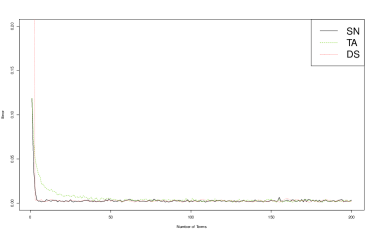
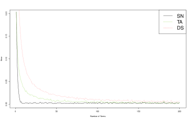
$\alpha=2,\beta=5$	$\alpha=5,\beta=1$

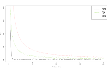
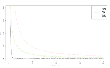
Figure 1: Plots of errors in the beta model with all three methods and several choices of the parameters. The $x$-axis represents $k$, the number of terms in the sum, and the $y$-axis represents the errors.

Our simulations are performed as follows. We begin by choosing values for $\alpha$ and $\beta$. We then select one of our three approximate simulation methods and a value for the tuning parameter $k$. Next, we use the method to approximately simulate $N$ observations from $\mathrm{MD}(\sigma^{\alpha,\beta})$. Using these, we estimate the means $m_{1}$, $m_{2}$ of both components, the variances $\sigma_{1}^{2}$, $\sigma^{2}_{2}$ of both components, and the covariance $\sigma_{12}$ between the components by using the empirical means $\bar{x}_{1}$, $\bar{x}_{2}$, the empirical variances $s_{1}^{2}$, $s_{2}^{2}$, and the empirical covariance $s_{12}$, respectively. We then quantify the error in the approximation by

$$\mathrm{E}_{k}=\sqrt{(\bar{x}_{1}-m_{1})^{2}+(\bar{x}_{2}-m_{2})^{2}+(s_{1}^{2}-\sigma_{1}^{2})^{2}+(s_{2}^{2}-\sigma_{2}^{2})^{2}+(s_{12}-\sigma_{12})^{2}}.$$ (17)

This was used to quantify errors in a similar context in [30]. The values of $m_{1}$, $m_{2}$, $\sigma_{1}^{2}$, $\sigma^{2}_{2}$, and $\sigma_{12}$ can be calculated by numerically integrating the formulas given in Section 4. When $\alpha$ and $\beta$ are integers, one can also evaluate the integrals explicitly using integration by parts. Note that only part of the error is due to the fact that the methods are approximate, the other part is due to Monte Carlo error as we are using only a finite number ($N$) of replications.

The results of our simulations are presented in Figure 1. Here we consider four combinations of the parameters $(\alpha,\beta)$: $(1,1)$, $(2,2)$, $(2,5)$, and $(5,1)$. For each method and each choice of the parameters, we let $k$ range from $1$ to $200$. In each case, we simulate $N=160000$ replications. Figure 1 presents the value of $k$ plotted against the error $\mathrm{E}_{k}$. When $\alpha=\beta=1$, which corresponds to a uniform distribution, the SN and DS methods have similar performance and the error deceases very quickly. In comparison, the error for TA decreases much slower. For the other cases, SN has the best performance, followed by TA, and then DS has the worst performance.

Next, we turn to our second model. Here $\sigma$ has a finite support, i.e, $\sigma=\sum_{i=1}^{r}a_{i}\delta_{s_{i}}$. For simplicity, we take $a_{i}=1/r$ for each $i=1,2,\dots,r$ and the $s_{i}$’s to be evenly spaced. We again quantify the error using $\mathrm{E}_{k}$ as given in (17) and use the formulas in Section 4 to calculate the means, variances, and the covariance. This time they are all finite sums. The results of our simulations are given in Figures 2 and 3. In Figure 2 we consider the case where $r=50$. Since the DS method is exact in this case, we just evaluate it once and plot the resulting error as a baseline. Note that, due to Monte Carlo error, this error is not zero. For the other methods, we see that the error in SN decays quickly as $k$ increases, whereas for TA it decays slower. To get an idea of how the performance of the methods depends on the number of terms $r$, in Figure 3 we consider the case where $r=2,20,100$. We can see that both SN and TA work better when $r$ is larger. We do not include DS in these simulations as it is exact in this case.

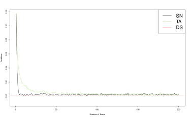
Figure 2: Plots of errors when $\sigma$ has $50$ evenly spaced directions. The $x$-axis represents $k$, the number of terms in the sum, and the $y$-axis represents the errors. Since DS is exact in this case, it is presented as a baseline.

SN	TA

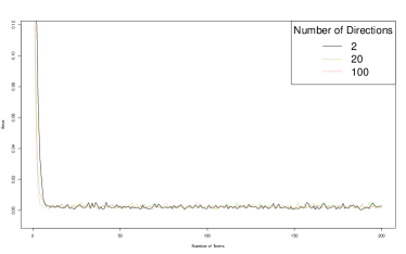
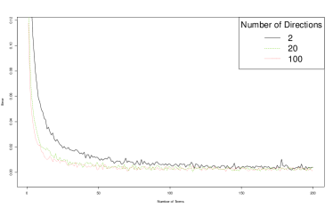
Figure 3: Plots of errors when $\sigma$ has $r=2,20,100$ evenly spaced directions. The plot of the left is for the SN method and the one on the right is for the TA method. The $x$-axis represents $k$, the number of terms in the sum, and the $y$-axis represents the errors. DS is not presented as it is exact in this case.

Overall, SN converges quickly in all of the situations that we considered. It is also easy to implement. TA is also easy to implement, but it needs more terms to converge. DS is an exact method when $\sigma$ has finite support. However, it is slightly harder to implement as it requires one to simulate GD random variables, which is a bit more involved.

6 Proofs

Proof of Lemma 1.

We get (6) from (4) by change of variables. Next, (6) implies that $M_{\alpha}(\mathbb{R}^{d})=\int_{\mathbb{R}^{d}}\int_{0}^{\infty}r^{\alpha-1}\mathrm{d}r\nu(\mathrm{d}x)$ and so $M_{\alpha}(\mathbb{R}^{d})=\infty$ for any $\nu\neq 0$. For the next part, note that, for $p>0$, l’Hôpital’s rule gives

$$\int_{a}^{\infty}r^{\alpha-1}e^{-rp}\mathrm{d}r\sim p^{-1}a^{\alpha-1}e^{-ap}\ \ \mbox{as}\ \ a\to\infty.$$

Thus, there exists a $K\geq e$ such that, if $|y|>K$, then

$$\frac{1}{2p}(\log|y|)^{\alpha-1}e^{-p\log|y|}\leq\int_{\log|y|}^{\infty}r^{\alpha-1}e^{-rp}\mathrm{d}r\leq\frac{2}{p}(\log|y|)^{\alpha-1}e^{-p\log|y|}.$$

Hence,

$$\int_{|x|\leq 1}|x|^{p}M_{\alpha}(\mathrm{d}x) = \int_{\mathbb{R}^{d}}|y|^{p}\int_{0}^{|y|^{-1}\wedge 1}(-\log r)^{\alpha-1}r^{p-1}\mathrm{d}r\nu(\mathrm{d}y)$$

$$= \int_{\mathbb{R}^{d}}|y|^{p}\int_{-\log(|y|^{-1}\wedge 1)}^{\infty}r^{\alpha-1}e^{-pr}\mathrm{d}r\nu(\mathrm{d}y)$$

$$\leq \int_{|y|\leq K}|y|^{p}\nu(\mathrm{d}y)\int_{0}^{\infty}r^{\alpha-1}e^{-pr}\mathrm{d}r+\frac{2}{p}\int_{|y|>K}(\log|y|)^{\alpha}\nu(\mathrm{d}y)$$

and similarly

$$\int_{|x|\leq 1}|x|^{p}M_{\alpha}(\mathrm{d}x) \geq \int_{|y|\leq K}|y|^{p}\nu(\mathrm{d}y)\int_{\log K}^{\infty}u^{\alpha-1}e^{-pr}\mathrm{d}r+\frac{1}{2p}\int_{|y|>K}(\log|y|)^{\alpha}\nu(\mathrm{d}y).$$

For the last part, we have

$$\int_{|x|>1}|x|^{p}M_{\alpha}(\mathrm{d}x) = \int_{|y|>1}|y|^{p}\int_{|y|^{-1}}^{1}(-\log r)^{\alpha-1}r^{p-1}\mathrm{d}r\nu(\mathrm{d}y)$$

$$= \int_{|y|>1}|y|^{p}\int_{0}^{\log|y|}r^{\alpha-1}e^{-pr}\mathrm{d}r\nu(\mathrm{d}y)$$

$$\leq \frac{\Gamma(\alpha)}{p^{\alpha}}\int_{|y|>1}|y|^{p}\nu(\mathrm{d}y)$$

and

$$\int_{|x|>1}|x|^{p}M_{\alpha}(\mathrm{d}x) = \int_{|y|>1}|y|^{p}\int_{0}^{\log|y|}r^{\alpha-1}e^{-pr}\mathrm{d}r\nu(\mathrm{d}y)$$

$$\geq \int_{|y|>e}|y|^{p}\nu(\mathrm{d}y)\int_{0}^{1}r^{\alpha-1}e^{-pr}\mathrm{d}r,$$

which completes the proof. ∎

Proof of Theorem 1..

Let $M_{\alpha}$ be as in (4) and let $C_{1}$ be the cgf of $Y_{1}$. By Corollary 2.3 in [25], the stochastic integral is absolutely definable so long as we have the finiteness of

$$\int_{0}^{\infty}\left|C_{1}\left(ze^{-(\alpha s/\theta)^{1/\alpha}}\right)\right|\mathrm{d}s$$

$$\qquad\leq|z||\gamma^{\prime}|\int_{0}^{\infty}e^{-(\alpha s/\theta)^{1/\alpha}}\mathrm{d}s+\theta^{-1}\int_{0}^{\infty}\int_{\mathbb{R}^{d}}1\wedge(|z||x|e^{-(\alpha s/\theta)^{1/\alpha}})\nu(\mathrm{d}x)\mathrm{d}s$$

$$\qquad\leq|z||\gamma^{\prime}|\int_{0}^{\infty}e^{-(\alpha s/\theta)^{1/\alpha}}\mathrm{d}s+\int_{\mathbb{R}^{d}}2\wedge(|z||x|)M_{\alpha}(\mathrm{d}x)<\infty,$$

where we use (6), (5), and the fact that $|e^{ia}-1|\leq 2\wedge|a|$ for $a\in\mathbb{R}$, see Section 26 in [2]. Similarly, by Proposition 2.2 in [25], the cgf of the stochastic integral is given by

$$\int_{0}^{\infty}C_{1}\left(ze^{-(\alpha s/\theta)^{1/\alpha}}\right)\mathrm{d}s$$

$$\qquad=\int_{0}^{\infty}\left(i\langle\gamma^{\prime},z\rangle e^{-(\alpha s/\theta)^{1/\alpha}}+\int_{\mathbb{R}^{d}}\left(e^{i\left\langle ze^{-(\alpha s/\theta)^{1/\alpha}},x\right\rangle}-1\right)\nu^{\prime}(\mathrm{d}x)\right)\mathrm{d}s$$

$$\qquad=i\langle\gamma^{\prime},z\rangle\int_{0}^{\infty}e^{-(\alpha s/\theta)^{1/\alpha}}\mathrm{d}s+\int_{\mathbb{R}^{d}}\left(e^{i\left\langle z,x\right\rangle}-1\right)M_{\alpha}(\mathrm{d}x).$$

From here, the result follows from the fact that $\int_{0}^{\infty}e^{-(\alpha s/\theta)^{1/\alpha}}\mathrm{d}s=\theta\Gamma(\alpha)$. ∎

Proof of Theorem 2.

The result follows by a general shot-noise representation of Lévy processes given in [23], see also Theorem 6.2 in [6]. Define

$$H(r,y)=ye^{-(r/\theta)^{1/\alpha}},\ \ r>0,\ y\in\mathbb{R}^{d}$$

and note that $|H(r,y)|$ is nonincreasing in $r$ for each $y$. Let

$$\lambda(r,B)=P(H(r,Y_{1})\in B)=P(Y_{1}\in e^{(r/\theta)^{1/\alpha}}B),\ \ r>0,\ B\in\mathfrak{B}(\mathbb{R}^{d}),$$

and

$$A(s)=\int_{0}^{s}\int_{|y|\leq 1}y\lambda(r,\mathrm{d}y)\mathrm{d}r,\ \ s\geq 0.$$

From (6) it follows that for $B\in\mathfrak{B}(\mathbb{R}^{d})$

$$\int_{0}^{\infty}\lambda(r,B)\mathrm{d}r = \int_{0}^{\infty}\int_{\mathbb{R}^{d}}1_{B}(ye^{-(r/\theta)^{1/\alpha}})\nu_{1}(\mathrm{d}y)\mathrm{d}r=M_{\alpha}(B).$$

and by dominated convergence that

$$\lim_{s\to\infty}A(s) = \int_{0}^{\infty}\int_{|y|\leq e^{(r/\theta)^{1/\alpha}}}ye^{-(r/\theta)^{1/\alpha}}\nu_{1}(\mathrm{d}y)\mathrm{d}r=\int_{|x|\leq 1}xM_{\alpha}(\mathrm{d}x).$$

We can use dominated convergence since by (5)

$$\int_{0}^{s}\int_{|y|\leq e^{(r/\theta)^{1/\alpha}}}|y|e^{-(r/\theta)^{1/\alpha}}\nu_{1}(\mathrm{d}y)\mathrm{d}r \leq \int_{0}^{\infty}\int_{|y|\leq e^{(r/\theta)^{1/\alpha}}}|y|e^{-(r/\theta)^{1/\alpha}}\nu_{1}(\mathrm{d}y)\mathrm{d}r$$

$$= \int_{|x|\leq 1}|x|M_{\alpha}(\mathrm{d}x)<\infty.$$

From here Theorem 6.2 in [6] gives the result for $T=1$. The results for general $T$ follows from the fact that the Lévy process $\{X_{t}:0\leq t\leq T\}$ where $X_{1}\sim\mathrm{ID}_{0}(M,\gamma)$ has the same distribution as $\{X^{\prime}_{t}:0\leq t\leq 1\}$ where $X^{\prime}_{1}\sim\mathrm{ID}_{0}(TM,T\gamma)$. The result for $\alpha=1$ follows from the well-known and easily checked fact that $e^{-E_{i}}\sim U(0,1)$. ∎

Proof of Theorem 3.

To prove this result, it suffices to verify the conditions for convergence of sums of infinitesimal triangular arrays. Such conditions can be found in, e.g., [24], [18], or [16]. A version of these is as follows:
1. For any $C\in\mathscr{B}(\mathbb{S}^{d-1})$ with $\nu\left(\left\{y\in\mathbb{R}^{d}\setminus\{0\}:\frac{y}{|y|}\in\partial C\right\}\right)=0$ and $s>0$, then

$$\lim_{n\to\infty}N_{n}\mathrm{P}\left(|T_{1}|X_{1}^{n}>s,\frac{T_{1}}{|T_{1}|}\in C\right)=M_{\alpha}\left(\left\{x\in\mathbb{R}^{d}:|x|>s,\frac{x}{|x|}\in C\right\}\right).$$

2.

$$\lim_{\epsilon\downarrow 0}\limsup_{n\to\infty}N_{n}\mathrm{E}\left[X_{1}^{n}|T_{1}|1(X_{1}^{n}|T_{1}|<\epsilon)\right]=0.$$

We begin by noting that, by L’Hôpital’s rule, for any $t>s>0$ we have

$$n\left(1-(s/t)^{1/n}\right)\sim\log(t/s).$$

Let $\ell_{0}(t)=\ell(1/t)$ and note that $\ell_{0}$ is slowly varying at $\infty$, i.e. for every $t>0$

$$\lim_{x\to\infty}\frac{\ell_{0}(xt)}{\ell_{0}(x)}=1.$$

Proposition 2.6 in [21] implies that for $t>s>0$ we have

$$\ell\left(1-(s/t)^{1/n}\right)=\ell_{0}\left(\frac{n}{n(1-(s/t)^{1/n})}\right)\sim\ell_{0}\left(n\right)=\ell(1/n)$$

and hence

$$\lim_{n\to\infty}N_{n}P(X_{1}>(s/t)^{1/n})=\lim_{n\to\infty}cn^{\alpha}(1-(s/t)^{1/n})^{\alpha}\frac{\ell(1-(s/t)^{1/n})}{\ell(1/n)}=c(\log(t/s))^{\alpha}.$$

By Theorem 20.3 in [2]

$$\lim_{n\to\infty}N_{n}\mathrm{P}\left(|T_{1}|X_{1}^{n}>s,\frac{T_{1}}{|T_{1}|}\in C\right) = \lim_{n\to\infty}\int_{|y|>s,\frac{y}{|y|}\in C}N_{n}P(X_{1}>(s/|y|)^{1/n})\nu_{0}(\mathrm{d}y)$$

$$= \int_{|y|>s,\frac{y}{|y|}\in C}\lim_{n\to\infty}N_{n}P(X_{1}>(s/t)^{1/n})\nu_{0}(\mathrm{d}y)$$

$$= c\int_{|y|>s,\frac{y}{|y|}\in C}\left(\log(|y|/s)\right)^{\alpha}\nu_{0}(\mathrm{d}y)$$

$$= M_{\alpha}\left(\left\{x\in\mathbb{R}^{d}:|x|>s,\frac{x}{|x|}\in C\right\}\right),$$

where in the second line we interchange limit and integration using dominated convergence. To see that we can do this, assume that $n$ is large enough that $N_{n}n^{-\alpha}\ell(1/n)\leq 2c$, let $t>s>0$, $a=\log(t/s)>0$, and fix $\delta\in(0,\alpha)$. By the Potter bounds, see e.g. Theorem 1.5.6 in [3], there exists a constant $A>0$ with

$$N_{n}P(X_{1}>(s/t)^{1/n}) \leq 2c\left(\frac{1-(s/t)^{1/n}}{1/n}\right)^{\alpha}\frac{\ell(1-(s/t)^{1/n})}{\ell(1/n)}$$ (18)

$$= 2c\left(\frac{1-e^{-a/n}}{1/n}\right)^{\alpha}\frac{\ell(1-e^{-a/n})}{\ell(1/n)}$$

$$\leq A\left(\left(\frac{1-e^{-a/n}}{1/n}\right)^{\alpha+\delta}\vee\left(\frac{1-e^{-a/n}}{1/n}\right)^{\alpha-\delta}\right)$$

$$\leq A\left((\log(t/s))^{\alpha+\delta}\vee(\log(t/s))^{\alpha-\delta}\right)\leq C_{s}t^{\gamma},$$

where $C_{s}$ is some constant depending on $s$ and we use the fact that $1-e^{-x}\leq x$. Next consider

$$\lim_{\epsilon\downarrow 0}\limsup_{n\to\infty}N_{n}\mathrm{E}\left[X_{1}^{n}|T_{1}|1_{[X_{1}^{n}|T_{1}|<\epsilon]}\right]$$

$$\qquad=\lim_{\epsilon\downarrow 0}\limsup_{n\to\infty}N_{n}\int_{0}^{\epsilon}P(X_{1}^{n}|T_{1}|1_{[X_{1}^{n}|T_{1}|<\epsilon]}>s)\mathrm{d}s$$

$$\qquad\leq\lim_{\epsilon\downarrow 0}\limsup_{n\to\infty}N_{n}\int_{0}^{\epsilon}P(X_{1}^{n}|T_{1}|>s)\mathrm{d}s$$

$$\qquad=\lim_{\epsilon\downarrow 0}\limsup_{n\to\infty}\int_{0}^{\epsilon}\int_{s\leq|y|}N_{n}P(X_{1}^{n}>s/|y|)\nu_{0}(\mathrm{d}y)\mathrm{d}s$$

$$\qquad\leq A\lim_{\epsilon\downarrow 0}\int_{|y|>0}\int_{0}^{\epsilon}\left((\log(|y|/s))^{\alpha+\delta}\vee(\log(|y|/s))^{\alpha-\delta}\right)\mathrm{d}s\nu_{0}(\mathrm{d}y)$$

$$\qquad=A\lim_{\epsilon\downarrow 0}\int_{|y|>0}\int_{\log(|y|/\epsilon)}^{\infty}\left(s^{\alpha+\delta}\vee s^{\alpha-\delta}\right)e^{-s}\mathrm{d}s|y|\nu_{0}(\mathrm{d}y)$$

$$\qquad\leq A\lim_{\epsilon\downarrow 0}\epsilon^{1-\gamma}\int_{|y|>0}\int_{\log(|y|/\epsilon)}^{\infty}\left(s^{\alpha+\delta}\vee s^{\alpha-\delta}\right)e^{-s\gamma}\mathrm{d}s|y|^{\gamma}\nu_{0}(\mathrm{d}y)$$

$$\qquad\leq A\lim_{\epsilon\downarrow 0}\epsilon^{1-\gamma}\int_{\mathbb{R}^{d}}|y|^{\gamma}\nu_{0}(\mathrm{d}y)\int_{0}^{\infty}\left(s^{\alpha+\delta}\vee s^{\alpha-\delta}\right)e^{-s\gamma}\mathrm{d}s=0,$$

where the fifth line follows by (18) and the sixth by change of variables. ∎

References

• [1] C. Bhattacharjee and I. Molchanov (2020). Convergence to scale-invariant Poisson processes and applications in Dickman approximation. Electronic Journal of Probability, 25, Article 79.
• [2] P. Billingsley (1995). Probability and Measure, 3rd ed. John Wiley & Sons, New York.
• [3] N.H. Bingham, C.M. Goldie, and J.L. Teugels (1987). Regular Variation. Encyclopedia of Mathematics And Its Applications. Cambridge University Press, Cambridge.
• [4] Z. Chi (2012). On exact sampling of nonnegative infinitely divisible random variables. Advances in Applied Probability, 44(3), 842-873.
• [5] K. Cloud and M. Huber (2017). Fast perfect simulation of Vervaat perpetuities. Journal of Complexity, 42, 19–30.
• [6] R. Cont and P. Tankov (2004). Financial Modeling With Jump Processes. CRC Press, Boca Raton.
• [7] S. Covo (2009). On Approximations of Small Jumps of Subordinators with Particular Emphasis on A Dickman-Type Limit. Journal of Applied Probability 46, 732-755
• [8] A. Dassios, Y. Qu, and J.W. Lim (2019). Exact simulation of generalised Vervaat perpetuities. Journal of Applied Probability, 56(1): 57–75.
• [9] L. Devroye (2001). Simulating Perpetuities. Methodology and Computing in Applied Probability, 3(1):97–115.
• [10] L. Devroye and O. Fawzi (2010). Simulating the Dickman distribution. Statistics & Probability Letters, 80(3-4):242–247.
• [11] J. Fill and M. Huber (2010). Perfect simulation of Vervaat perpetuities. Electronic Journal of Probability, 15(4):96–109.
• [12] M. Grabchak and L. Cao (2023). SubTS: Positive Tempered Stable Distributions and Related Subordinators. Ver. 1.0, R Package.https://CRAN.R-project.org/package=SubTS.
• [13] M. Grabchak and S.A. Molchanov (2019). Limit theorems for random exponentials: The bounded support case. Theory of Probability and its Applications 63(4), 634-647
• [14] M. Grabchak, S.A. Molchanov, and V.A. Panov (2022). Around the infinite divisibility of the Dickman distribution and related topics. Zapiski Nauchnykh Seminarov POMI, 115:91-120.
• [15] Z.J. Jurek (1999). Selfdecomposability perpetuity laws and stopping times. Probability and Mathematical Statistics, 19(2):413–419.
• [16] O. Kallenberg (2002). Foundations of Modern Probability, 2nd Ed. Springer-Verlag, New York.
• [17] M. Maejima and Y. Ueda (2010) $\alpha$-selfdecomposable distributions and related Ornstein–Uhlenbeck type processes. Stochastic Processes and their Applications, 120(12):2363–2389.
• [18] M. Meerschaert and H. Scheffler (2001). Limit Distributions for Sums of Independent Random Vectors: Heavy Tails in Theory and Practice. Wiley, New York
• [19] S.A. Molchanov and V.A. Panov (2020). The Dickman–Goncharov distribution. Russian Mathematical Surveys, 75(6), 1089.
• [20] M. Penrose and A. Wade (2004). Random minimal directed spanning trees and Dickman-type distributions. Advances in Applied Probability 36(3):691–714.
• [21] S. Resnick (2007). Heavy-Tail Phenomena Probabilistic and Statistical Modeling. Springer, New York
• [22] A. Rocha-Arteaga and K. Sato (2019). Topics in infinitely divisible distributions and Lévy processes, Revised Edition. Springer, Cham
• [23] J. Rosiński (2001). Series representations of Levy processes from the perspective of point processes. In Levy Processes – Theory and Applications. O.E. Barndorff-Nielsen, T. Mikosch and S.I. Resnick, Eds., Birkhauser, Boston, pp. 401–415.
• [24] K. Sato (1999). Lévy Processes and Infinitely Divisible Distributions. Cambridge University Press, Cambridge.
• [25] K. Sato (2006). Two families of improper stochastic integrals with respect to Lévy processes. ALEA Latin American Journal of Probability and Mathematical Statistics, 1, 47–87.
• [26] K. Sato (2010). Fractional integrals and extensions of selfdecomposability. In: Barndorff-Nielsen, O., Bertoin, J., Jacod, J., Klüppelberg, C. (eds) Lévy Matters I. Lecture Notes in Mathematics, vol 2001. Springer, Berlin, Heidelberg.
• [27] M. Schlather (2001). Limit distributions of norms of vectors of positive i.i.d. random variables. Annals of Probability, 29(2):862–881.
• [28] N.V. Thu (1982). Universal multiply self-decomposable probability measures on Banach spaces. Probability and Mathematical Statistics, 3(2):71–84.
• [29] W. Vervaat (1979). On a stochastic difference equation and a representation of non-negative infinitely divisible random variables. Advances in Applied Probability, 11(4), 750–783.
• [30] Y. Xia and M. Grabchak (2022). Estimation and simulation for multivariate tempered stable distributions. Journal of Statistical Computation and Simulation, 92(3):451–475.