Experience Filter: Using Past Experiences on
Unseen Tasks or Environments

Abstract

One of the bottlenecks of training autonomous vehicle (AV) agents is the variability of training environments. Since learning optimal policies for unseen environments is often very costly and requires substantial data collection, it becomes computationally intractable to train the agent on every possible environment or task the AV may encounter.

This paper introduces a zero-shot filtering approach to interpolate learned policies of past experiences to generalize to unseen ones. We use an experience kernel to correlate environments. These correlations are then exploited to produce policies for new tasks or environments from learned policies. We demonstrate our methods on an autonomous vehicle driving through T-intersections with different characteristics, where its behavior is modeled as a partially observable Markov decision process (POMDP). We first construct compact representations of learned policies for POMDPs with unknown transition functions given a dataset of sequential actions and observations. Then, we filter parameterized policies of previously visited environments to generate policies to new, unseen environments. We demonstrate our approaches on both an actual AV and a high-fidelity simulator. Results indicate that our experience filter offers a fast, low-effort, and near-optimal solution to create policies for tasks or environments never seen before. Furthermore, the generated new policies outperform the policy learned using the entire data collected from past environments, suggesting that the correlation among different environments can be exploited and irrelevant ones can be filtered out.

I Introduction

Designing efficient and safe planning strategies for autonomous vehicles is generally challenging due to uncertainty. One of the principled ways of modeling the planning problem under uncertainty is using POMDPs [kaelbling1998planning], which have been successfully applied in autonomous driving [cailets, sunberg_pomdp]. The POMDP formulation includes a state transition model which represents the environment dynamics. When this model is not readily available for a given problem, machine learning techniques can be used to learn the environment models from data collected at design time. Although reinforcement learning algorithms have been shown to produce effective policies for environments that they are trained upon [kochenderfer2015_dmu], they typically need to be retrained to be deployed in new environments. To overcome this limitation, models or policies previously learned need to be transferred to new, unforeseen tasks.

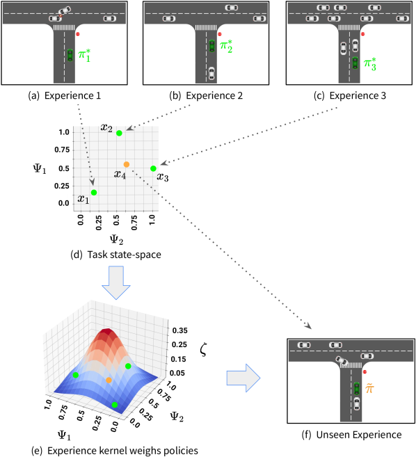
Figure 1: (a)-(d) Different tasks or environments $x_{i}\in\mathcal{X}$ (and their policies $\pi_{i}^{*}$) can be compactly represented through parameterization. (e) Here, we define the relationship between a new environment (parameterized by $x_{4}$) and previously visited environments (parameterized by $x_{1},x_{2},x_{3}$) using a kernel $\zeta(x_{m},x_{4})$, $m=\{1,2,3\}.$ (f) An experience filter exploits this relation to generate a policy for $x_{4}$ given policies trained on different tasks or environments.

In this work, we introduce the concept of an experience filter, illustrated in Fig. 1, to reason about new tasks or environments using past experiences. The goal of the experience filter is to filter optimal/learned policies of previously visited environments to generate policies to ones never seen before. By doing so, we eliminate the need to train an autonomous vehicle’s policy on a vast range of different tasks, but rather, interpolate existing policies to unseen similar tasks, eliminating the need to collect any new data. Our experience filter (EF) approach allows fast, low-effort, and near-optimal solutions to create policies without requiring to train for tasks or environments not seen before. Furthermore, our results also indicate that using the EF approach to correlate and filter previous experiences through a kernel, as depicted in Fig. 1, yields higher performance than simply using the entire data collected in an attempt to train an all-for-one policy.

We assume that both policies and environments can be represented by low-dimensional, easily accessible parameter vectors. For example, the behavior of an AV navigating along a highway can be influenced by factors such as traffic density, number of lanes, upcoming intersections, etc. Our proposed experience filter takes environment representations and parameterized policies as an input, and using an experience kernel, outputs a new policy for an unseen environment through Bayesian reasoning between the learned and unseen environment parameters.

The contributions of this paper are twofold: (1) we introduce a new technique to learn and parameterize policies of a POMDP with an unknown transition function from existing data, and (2) we propose an experience filter to efficiently plan in unseen environments by interpolating past knowledge. We demonstrate our approach on a problem of autonomously driving through T-intersections, and we include demonstrations on both an actual AV and a high-fidelity simulator CARLA [carla-sim]. For simulation results, we benchmark our experience filter approach using the following performance metrics: collision risk, discomfort during driving, and task completion time.

The paper is organized as follows: Section II gives an overview of transfer learning techniques. Section III gives a brief background on Dirichlet distributions, POMDPs, and MODIA and Section IV defines the problem. Section V presents our learning approach and experience filter. LABEL:sec:results summarizes results. Finally, LABEL:sec:conclusion draws conclusions and discusses future work.

II Related Work

The problem of how to reduce training effort for new tasks by leveraging the knowledge from existing tasks has been addressed by transfer learning techniques. Existing work on transfer learning techniques largely focuses on transferring knowledge from previously seen source tasks to new tasks [zhuang2020comprehensive] and can be divided into the following three categories.

Model-free transfer

Transfer learning for model-free reinforcement learning algorithms involves transferring knowledge between tasks in the form of experience samples, policies, or value functions. Progressive networks [rusu2016progressive] is an approach to transfer learning where additional neurons are added to a network for each new task that is learned. Previously learned network weights are frozen, and the new neurons are connected so as not to change the output of the network on previous tasks. The attend, adapt, and transfer approach [rajendran2017attend] uses a set of attention weights to combine the output of a set of source policies to achieve good performance on a new task. To avoid negative transfer, a new policy is learned from scratch and combined with the source policies through an additional weight. The attention weights can be learned from a small amount of data, allowing for fast adaptation to new environments. Transfer learning with model-free deep reinforcement learning is also applied to task transfer for autonomous driving decision making problems [shu-itvt-2022].

Model-based transfer

Prior work on transfer in a model-based setting assumes there are unobserved parameters that describe each task and seek to learn a model of these parameters from data [chrisman1992reinforcement, choi1999environment]. Recent work [killian2017robust] assumes a low-dimensional latent task identifier which is inferred online using a Bayesian neural network, allowing for fast adaptation to new problems. Hidden parameter MDPs were extended to allow for variations in the reward function [perez2020generalized]. Storing experience samples from previous source tasks and constructing a model for the new task with an inter-task mapping has also been done [taylor2008transferring]. Our approach is similar to the aforementioned work in that transfer to a new task is done by combining previously learned models. Both model-based and model-free approaches, however, require training on the new task, whereas we consider the case of zero-shot transfer in this paper.

Zero-shot transfer

Zero-shot transfer [wang2019survey] is often preferred when there is a known relationship between tasks. For example, when the source task is a simulated version of the real target task, unsupervised pre-training has shown to be effective for enabling zero-shot transfer [higgins2017darla]. Alternatively, automated measures of MDP similarity can be used [ammar2014automated]. Zero-shot policy transfer along with the robust tracking controllers to tackle the source to target modeling gap is applied in robotics [harrison2020adapt] and autonomous driving problems [xu2018zero]. In our setting, we exploit a parametric connection between previously visited environments, using this relation to hypothesize policies for unseen environments.

III Background

III-A Dirichlet Distributions

Dirichlet distribution $\text{Dir}\left(\boldsymbol{\alpha}_{1:n}\right)$ is parameterized by $\boldsymbol{\alpha}_{1:n}\in\mathbb{R}_{\geq 0}^{n}$ which can be treated as pseudo-counts of different outcomes. The density of a Dirichlet distribution is given by

$$P\left(\boldsymbol{\theta}_{1:n}\mid\boldsymbol{\alpha}_{1:n}\right)=\dfrac{\Gamma\left(\sum_{i=1}^{n}\alpha_{i}\right)}{\prod_{i=1}^{n}\Gamma\left(\alpha_{i}\right)}\prod_{i=1}^{n}\theta_{i}^{\alpha_{i}-1}$$

where $\Gamma$ is the gamma function [kotz2004continuous].

If the prior is a Dirichlet distribution and the event $i$ is observed $m_{i}\in\boldsymbol{m}_{1:n}$ times, then the posterior is also a Dirichlet distribution [kochenderfer2015_dmu]:

$$\boldsymbol{\theta}_{1:n}\mid\boldsymbol{\alpha}_{1:n},\boldsymbol{m}_{1:n}\sim\text{Dir}\left(\boldsymbol{\alpha}_{1:n}+\boldsymbol{m}_{1:n}\right).$$

III-B Partially Observable Markov Decision Processes

A sequential decision making problem can be modeled as a partially observable Markov decision process. A POMDP model is represented by a tuple $\langle\mathcal{S},\mathcal{A},\mathcal{O},T,Z,R,\gamma\rangle$ where $\mathcal{S}$ is a finite set of states, $\mathcal{A}$ is a finite set of actions, and $\mathcal{O}$ is a finite state of observations. The system takes an action $a\in\mathcal{A}$ from state $s\in\mathcal{S}$ and transitions to the next state $s^{\prime}\in\mathcal{S}$ according to the probabilistic transition function $T(s^{\prime}\mid s,a)=P(s^{\prime}\mid s,a)$ which models the environment dynamics. From state $s^{\prime}$ the system obtains observation $o\in\mathcal{O}$ according to the observation function $Z(o\mid s^{\prime},a)=P(o\mid s^{\prime},a)$ and receives a reward according to the reward function $R(s,a)$. As the system does not have access to the true world states, it maintains a belief $b(s)$ over possible states. A discount factor $\gamma\in[0,1]$ may also be used to prioritize earning rewards sooner than later.

The goal of the system is to find a policy $\pi^{*}$ to maximize the expected total discounted reward starting from its belief $b$, which can be exactly calculated using the relation

$$\pi^{*}(b)=\operatorname*{arg\,max}_{a}\sum_{s}b(s)Q(s,a)$$ (1)

where

$$V^{*}(b)=\max_{a}\sum_{s}b(s)Q(s,a)$$ (2)

$$\begin{split}Q(s&,a)=R(s,a)\\ &+\gamma\sum_{s^{\prime}}T(s^{\prime}\mid s,a)\sum_{o}Z(o\mid s^{\prime},a)V^{*}(b^{\prime}_{(b,a,o)})\end{split}$$ (3)

and $b^{\prime}_{(b,a,o)}$ is the updated belief.

$$\begin{gathered}\boldsymbol{m}_{(s,a)}=\begin{bmatrix}m_{(s,a,s_{1}^{\prime})}\\ m_{(s,a,s_{2}^{\prime})}\\ \vdots\\ m_{(s,a,s_{|\mathcal{S}|}^{\prime})}\end{bmatrix}\quad\text{where}\quad m_{(s,a,s^{\prime})}=\sum_{S_{k}\in\mathcal{D}_{i}}\sum_{C_{j}\in S_{k}}\sum_{{(s_{ijk},a_{ijk},s^{\prime}_{ijk})}\in C_{j}}\int_{t=0}^{t=\tau_{k}}\mathbf{1}\begin{Bmatrix}s_{ijk}(t)=s\\ a_{ijk}(t)=a\\ s^{\prime}_{ijk}(t)=s^{\prime}\end{Bmatrix}dt\end{gathered}$$ (5)

For fully observable states (MDP), the belief and observation terms in Eqs. 1, 2 and 3 drop out, and the optimal solution can be computed tractably using Bellman updates [bellman2015applied]. However, finding a solution to a POMDP using dynamic programming is computationally very expensive, and thus, approximate solutions are often used instead [kochenderfer2015_dmu]. In this work, we use the QMDP [hauskrecht2000value] offline solver, and assume the resulting policy to be near-optimal.

III-C MODIA

The multiple online decision-components with interacting actions (MODIA) framework [ijcai2017-664] aims to solve complicated real world decision making problems in a scalable way by separating them into subproblems. Instead of constructing a single POMDP that accounts for all of the other agents in a domain, MODIA instantiates multiple smaller POMDPs for each agent interaction. This formulation inherently assumes that most agents act independently from one another. At each timestep, the safest action among all POMDPs is selected for execution. MODIA is utilized during the experimentation.

IV Problem Definitions

In this study, our goal is to efficiently generate new policies for unseen driving tasks or environments using past experiences. To achieve this, we need to represent policies by a compact representation, and then find a way to transfer the policies. These two problems are defined as follows:

Problem 1: Parameterizing Policies: Given a driving dataset $\mathcal{D}_{i}$ containing observation triplets $(o^{t}_{i},a^{t}_{i},o^{t+1}_{i})$ obtained from $N$ different driving environments visited at times $t\in[0,\tau_{i}]$, and a policy $\pi_{i}^{*}$ learned for environment $i$, what is the compact representation $par(\pi_{i}^{*})$ of this policy?

Problem 2: Experience Transfer: Given a set of policy representations $par(\pi^{*}_{i}),\ i=1,\dots,N$ learned for $N$ visited environments, how can we compute a reasonable policy for an environment that was never seen before?

In this paper, we investigate the behavior of an AV at T-intersections. We model the AV’s behavior as a POMDP, and assume that the $Z(o\mid s^{\prime},a)$ and $R(s,a)$ functions are known. In the first portion of this paper, we focus on learning the transition function $T(s^{\prime}\mid s,a)$ for T-intersections of different characteristics. Given that $T$, $Z$ and $R$ are learned or known, the optimal policy of the POMDP can therefore be solved for from Eqs. 1, 2 and 3. In the second portion of this paper, we introduce a framework that allows us to deduce a policy for a T-intersection type that was never seen before, by generalizing a handful number of previously learned policies. We discuss our approaches to both of these problems in Section V.

V Efficient Transition Function Learning and Transferring

In this section, we first discuss how the policy is learned for an individual T-intersection. Then, the experience filter, that allows computing a policy for unseen T-intersection types, is formulated.

V-A Learning and Parameterizing the Policy

The $\mathcal{S}$, $\mathcal{A}$, $\mathcal{O}$ of the POMDP used to model the AV’s behavior at a T-intersection while considering a single rival vehicle is defined as follows.

State Space $\mathcal{S}$: Each state $s\in\mathcal{S}$ is a 5-dimensional $(pos_{ego},\ sgt_{ego},\ pos_{rival},\ blk_{rival},\ aggr_{rival})$ vector. Here, $pos_{ego},\ pos_{rival}\in\{\texttt{before},\ \texttt{at},\ \texttt{inside},\ \texttt{after}\}$ denote the position of the ego and rival vehicles with respect to the stop sign of the T-intersection, respectively, $sgt_{ego}\in\{\texttt{yes},\ \texttt{no}\}$ denotes whether or not the ego vehicle has a clear line of sight, $blk_{rival}\in\{\texttt{yes},\ \texttt{no}\}$ denotes whether or not the rival vehicle is blocking the ego vehicle’s path, $aggr_{rival}\in\{\texttt{cautious},\ \texttt{normal},\ \texttt{aggressive}\}$ denotes the aggressiveness level of the rival vehicle. Since all five dimensions of the state space are discretized, there are a total of $192$ possible states in $\mathcal{S}$.

Action Space $\mathcal{A}$: Consists of three permissible actions of the AV, which are $\{\texttt{stop},\ \texttt{edge},\ \texttt{go}\}$.

Observation Space $\mathcal{O}$: The observation space is equivalent to the state space $\mathcal{S}$, and therefore also has a cardinality of $192$. Note that observation $o$ is noisy over the true state $s$.

In this study, we assume that the observation and reward functions, $Z(o\mid s^{\prime},a)$ and $R(s,a)$, are known and constant across different types of T-intersections. This is a reasonable assumption since $Z$ inherently captures the sensing accuracy, and $R$ describes driving preferences, both of which can be quantitatively modeled a priori. Therefore, by inspecting Eqs. 1, 2 and 3, learning a policy for a specific T-intersection reduces to an accurate representation of the transition function $T(s^{\prime}\mid s,a)$.

In this study, we represent the learned transition function $\tilde{T}$ as the posterior Dirichlet distribution:

$$\boldsymbol{\theta}(s,a)\sim\text{Dir}\left(\boldsymbol{\alpha}_{(s,a)}+\boldsymbol{m}_{(s,a)}\right)$$ (4)

where $\boldsymbol{\theta}(s,a)\in\left[0,1\right]^{|\mathcal{S}|}$ is a vector whose each element is $\theta(s,a)=\tilde{T}(s^{\prime}\mid s,a),\ \forall s^{\prime}\in\mathcal{S}$, given $s,a$. Parameters $\boldsymbol{\alpha}_{(s,a)}\in\mathbb{R}_{\geq 0}^{|\mathcal{S}|}$, and $\boldsymbol{m}_{(s,a)}\in\mathbb{Z}_{+}^{|\mathcal{S}|}$ describe the prior and likelihood pseudo-counts, respectively.

A dataset $\mathcal{D}_{i}$ is collected as a specific intersection $i$ is driven through $d$ times. We call each drive through an intersection a scenario, hence, there are $d$ scenarios in $\mathcal{D}_{i}$. During each scenario $S_{k}$, the ego vehicle interacts with multiple rival cars and receives observation triplets, each of them labeled $C_{j}$. As a part of the MODIA definition (Section III-C), a separate PODMP is instantiated for each rival car at the T-intersection. These instantiated POMDPs may use a baseline or expert policy (if available). As a result, separate $(s,a,s^{\prime})$ triplets are recorded for each rival vehicle. Therefore, the likelihood pseudo-counts $\boldsymbol{m}_{(s,a)}$ can be formulated as in Eq. 5 where $\tau_{k}$ denotes the total time taken in scenario $S_{k}$, and $\mathbf{1}\{\cdot\}$ outputs a scalar $1$ if all expressions inside the curly braces are true, and $0$ otherwise. However, due to partial observability, we cannot directly observe the states, but rather, receive observations from the world, making Eq. 5 inaccessible for POMDPs. Furthermore, the integral in Eq. 5 is often intractable. As a remedy, we use the most likely state with respect to the observations received, and discretize the scenarios into small timesteps:

$$m_{(s,a,s^{\prime})}=\sum_{S_{k}\in\mathcal{D}_{i}}\sum_{C_{j}\in S_{k}}\sum_{{(o_{ijk}^{t},a_{ijk}^{t},o_{ijk}^{t+1})}\in C_{j}}\sum_{t=0}^{\tau_{k}}\mathbf{1}\begin{Bmatrix}\tilde{s}_{ijk}^{t}=s\\ a_{ijk}^{t}=a\\ \tilde{s}_{ijk}^{t+1}=s^{\prime}\end{Bmatrix}$$ (6)

where

$$\tilde{s}^{t+1}_{ijk} =\operatorname*{arg\,max}_{s}b_{ijk}^{t+1}(s)$$

$$b_{ijk}^{t+1}(s) =P(s\mid b_{ijk}^{t},a_{ijk}^{t},o_{ijk}^{t}).$$

We represent a learned policy $\pi^{*}$ through a set of parameters $par(\pi^{*})$. For POMDP representations, through Eqs. 1, 2 and 3, the optimal policy depends on $T$, $Z$ and $R$. As previously mentioned, we are treating $Z$ and $R$ to be known a priori, and assumed to be constant across different T-intersection characteristics. Hence, we can readily accept the parameters that describe a learned policy in our AV domain to be $T(s^{\prime}\mid s,a),\ \forall a\in\mathcal{A},\ \forall s^{\prime},s\in\mathcal{S}$. From this logic, $par(\pi_{i}^{*})$ for intersection $i$ is distributed by the product

$$par(\pi_{i}^{*})\sim\prod_{s}\prod_{a}\text{Dir}\left(\boldsymbol{\alpha}_{(s,a)}+\boldsymbol{m}_{(s,a)}\right)$$ (7)

and contains $|\mathcal{S}|^{2}\times|\mathcal{A}|=192^{2}\times 3=110,592$ parameters.

V-B Experience Filter

We first define the environment state-space $\mathcal{X}$ and experience kernel $\zeta(\cdot)$ as follows.

Definition V.1

Let a set of parameters $(\psi_{1},\cdots,\psi_{K})$ where $\psi_{k}\in\Psi_{k},\ k=1,...,K$ efficiently represent an environment. Then, an environment state-space is the Cartesian product $\mathcal{X}=\Psi_{1}\times\cdots\times\Psi_{K}$ which can be defined as

$$\mathcal{X}=\left\{(\psi_{1},\cdots,\psi_{K})\mid\psi_{k}\in\Psi_{k},\ k=1,...,K\right\}.$$ (8)