Maximize to Explore: One Objective Function Fusing Estimation, Planning, and Exploration

Abstract

In online reinforcement learning (online RL), balancing exploration and exploitation is crucial for finding an optimal policy in a sample-efficient way. To achieve this, existing sample-efficient online RL algorithms typically consist of three components: estimation, planning, and exploration. However, in order to cope with general function approximators, most of them involve impractical algorithmic components to incentivize exploration, such as optimization within data-dependent level-sets or complicated sampling procedures. To address this challenge, we propose an easy-to-implement RL framework called Maximize to Explore (MEX), which only needs to optimize unconstrainedly a single objective that integrates the estimation and planning components while balancing exploration and exploitation automatically. Theoretically, we prove that MEX achieves a sublinear regret with general function approximations for Markov decision processes (MDP) and is further extendable to two-player zero-sum Markov games (MG). Meanwhile, we adapt deep RL baselines to design practical versions of MEX, in both model-free and model-based manners, which can outperform baselines by a stable margin in various MuJoCo environments with sparse rewards. Compared with existing sample-efficient online RL algorithms with general function approximations, MEX achieves similar sample efficiency while enjoying a lower computational cost and is more compatible with modern deep RL methods. Our codes are available at https://github.com/agentification/MEX.

1 Introduction

The crux of online reinforcement learning (online RL) lies in maintaining a balance between i) exploiting the current knowledge of the agent about the environment and ii) exploring unfamiliar areas (Sutton and Barto, 2018). To fulfill this, agents in existing sample-efficient RL algorithms predominantly undertake three tasks: i) estimate a hypothesis using historical data to encapsulate their understanding of the environment; ii) perform planning based on the estimated hypothesis to exploit their current knowledge; iii) further explore the unknown environment via carefully designed exploration strategies.

There exists a long line of research on integrating the aforementioned three components harmoniously to find the optimal policy in a sample-efficient manner. From theoretical perspectives, existing theories aim to minimize the notion of online external regret which measures the cumulative suboptimality gap of the policies learned during online learning. It is well studied that one can design both statistically and computationally efficient algorithms (e.g., upper confidence bound (UCB), Azar et al. (2017); Jin et al. (2020b); Cai et al. (2020); Zhou et al. (2021)) with sublinear online regret for tabular and linear Markov decision processes (MDPs). But when it comes to MDPs with general function approximations, most of them involve impractical algorithmic components to incentivize exploration. Usually, to cope with general function approximations, agents need to solve constrained optimization problems within data-dependent level-sets (Jin et al., 2021a; Du et al., 2021), or sample from complicated posterior distributions over the space of hypotheses (Dann et al., 2021; Agarwal and Zhang, 2022; Zhong et al., 2022), both of which pose considerable challenges for implementation. From a practical perspective, a prevalent approach in deep RL for balancing exploration and exploitation is to use an ensemble of neural networks (Wiering and Van Hasselt, 2008; Osband et al., 2016; Chen et al., 2017; Lu and Van Roy, 2017; Kurutach et al., 2018; Chua et al., 2018; Lee et al., 2021), which serves as an empirical approximation of the UCB method. However, such an ensemble method suffers from high computational cost and lacks a theoretical guarantee when the underlying MDP is neither linear nor tabular. As for other deep RL algorithms for exploration (Haarnoja et al., 2018a; Aubret et al., 2019; Burda et al., 2018; Bellemare et al., 2016; Choi et al., 2018), such as the curiosity-driven method (Pathak et al., 2017), it also remains unknown in theory whether they are provably sample-efficient in the context of general function approximations.

Hence, in this paper, we are aimed at tackling these issues and answering the following question:

Under general function approximation, can we design a sample-efficient and
easy-to-implement RL framework to trade off between exploration and exploitation?

Towards this goal, we propose an easy-to-implement RL framework, Maximize to Explore (MEX), as an affirmative answer to above question. In order to strike a balance between exploration and exploitation, MEX propose to maximize a weighted sum of two objectives: (a) the optimal expected total return associated with a given hypothesis, and (b) the negative estimation error of that hypothesis. Consequently, MEX naturally combines planning and estimation components in just one single objective. By choosing the hypothesis that maximizes the weighted sum and executing the optimal policy with respect to the chosen hypothesis, MEX automatically balances between exploration and exploitation.

We highlight that the objective of MEX is not obtained through the Lagrangian duality of the constrained optimization objective within data-dependent level-sets (Jin et al., 2021a; Du et al., 2021; Chen et al., 2022b). This is because the coefficient of the weighted sum, which remains fixed, is data-independent and predetermined for all episodes. Contrary to the Lagrangian duality, MEX does not necessitate an inner loop of optimization for dual variables, thereby circumventing the complications associated with minimax optimization. As a maximization-only framework, MEX is friendly to implementations with neural networks and does not rely on sampling or ensemble.

In the theory part, we prove that MEX achieves a sublinear $\widetilde{\mathcal{O}}(\texttt{Poly}(H)d_{\text{GEC}}^{1/2}(1/\sqrt{HK})K^{1/2})$ regret under mild structural assumptions and is thus sample-efficient. Here $K$ is the number of episodes, $H$ is the horizon length, and $d_{\text{GEC}}(\cdot)$ is the Generalized Eluder Coefficient (GEC) (Zhong et al., 2022) that characterizes the complexity of learning the underlying MDP using general function approximations in the online setting. Because the class of low-GEC MDPs includes almost all known theoretically tractable MDP instances, our result can be tailored to a multitude of specific settings with either a model-free or a model-based hypothesis, such as MDPs with low Bellman eluder dimension (Jin et al., 2021a), MDPs of bilinear class (Du et al., 2021), and MDPs with low witness rank (Sun et al., 2019). Thanks to the flexibility of the MEX framework, we further extend it to online RL in two-player zero-sum Markov games (MGs), for which we also generalize the definition of GEC to two-player zero-sum MGs and establish the sample efficiency with general function approximations. Finally, as the low-GEC class also contains many tractable Partially Observable MDP (POMDP) classes (Zhong et al., 2022), MEX can also be applied to these POMDPs.

Moving beyond theory and into practice, we adapt famous RL baselines TD3 (Fujimoto et al., 2018) and MBPO (Janner et al., 2019) to design practical versions of MEX in model-free and model-based fashion, respectively. On various MuJoCo environments (Todorov et al., 2012) with sparse rewards, experimental results show that MEX outperforms baselines steadily and significantly. Compared with other deep RL algorithms, MEX has low computational overhead and easy implementation while maintaining a theoretical guarantee.

1.1 Main Contributions

We conclude our main contributions from the following three perspectives.

1. We propose an easy-to-implement RL algorithm framework MEX that unconstrainedly maximizes a single objective to fuse estimation and planning, automatically trading off between exploration and exploitation. Under mild structural assumptions, we prove that MEX achieves a sublinear regret

   $$\widetilde{\mathcal{O}}\Big{(}\texttt{Poly}(H)\cdot d_{\text{GEC}}(1/\sqrt{HK})^{\frac{1}{2}}\cdot K^{\frac{1}{2}}\Big{)}$$

   with general function approximators, and thus is sample-efficient. Here $K$ denotes the number of episodes, $\texttt{Poly}(H)$ is a polynomial term in horizon length $H$ which is specified in Section 5, $d_{\text{GEC}}(\cdot)$ is the Generalized Eluder Coefficient (GEC) (Zhong et al., 2022) of the underlying MDP.

2. We instantiate the generic MEX framework to solve several model-free and model-based MDP instances and establish corresponding theoretical results. Beyond MDPs, we further extend the MEX framework to two-player zero-sum MGs and also prove the sample efficiency with an extended definition of GEC.

3. We design deep RL implementations of MEX in both model-free and model-based styles. Experiments on various MuJoCo environments with sparse rewards demonstrate the effectiveness of MEX framework.

1.2 Related Works

Sample-efficient RL with function approximation.

The success of DRL methods has motivated a line of works focused on function approximation scenarios. This line of works is originated in the linear function approximation case (Wang et al., 2019; Yang and Wang, 2019; Cai et al., 2020; Jin et al., 2020b; Zanette et al., 2020a; Ayoub et al., 2020; Yang et al., 2020; Modi et al., 2020; Zhou et al., 2021; Zhong and Zhang, 2023) and is later extended to general function approximations. Wang et al. (2020) first study the general function approximation using the notion of eluder dimension (Russo and Van Roy, 2013), which takes the linear MDP (Jin et al., 2020b) as a special case but with inferior results. Zanette et al. (2020b) consider a different type of framework based on Bellman completeness, which assumes that the class used for approximating the optimal Q-functions is closed in terms of the Bellman operator and improves the results for linear MDP. After this, Jin et al. (2021a) consider the eluder dimension of the class of Bellman residual associated with the RL problems, which captures more solvable problems (low Bellman eluder (BE) dimension). Another line of works focuses on the low-rank structures of the problems, where Jiang et al. (2017a) propose the Bellman rank for model-free RL and Sun et al. (2019) propose the witness rank for model-based RL. Following these two works, Du et al. (2021) propose the bilinear class, which contains more MDP models with low-rank structures (Azar et al., 2017; Sun et al., 2019; Jin et al., 2020b; Modi et al., 2020; Cai et al., 2020; Zhou et al., 2021) by allowing a flexible choice of discrepancy function class. However, it is known that neither BE nor bilinear class captures each other. Dann et al. (2021) first consider eluder-coefficient-type complexity measure on the Q-type model-free RL. It was later extended by Zhong et al. (2022) to cover all the above-known solvable problems in both model-free and model-based manners. Foster et al. (2021, 2023) study another notion of complexity measure, the decision-estimation coefficient (DEC), which also unifies the BE dimension and bilinear class and is appealing due to the matching lower bound in some decision-making problems but may not be applied to the classical optimism-based or sampling-based methods due to the presence of a minimax subroutine in the definition. Chen et al. (2022a); Foster et al. (2022) extend the vanilla DEC by incorporating an optimistic modification. Chen et al. (2022b) study Admissible Bellman Characterization (ABC) class to generalize BE. They also extend the GOLF algorithm (Jin et al., 2021a) and the Bellman completeness in model-free RL by considering more general (vector-form) discrepancy loss functions and obtaining sharper bounds in some problems. Xie et al. (2022) connect the online RL with the coverage condition in the offline RL, and also study the GOLF algorithm proposed in Jin et al. (2021a).

Algorithmic design in sample-efficient RL with function approximation.

The most prominent approach in this area is based on the principle of “Optimism in the Face of Uncertainty” (OFU), which dates back to Auer et al. (2002). For instance, for linear function approximation, Jin et al. (2020b) propose an optimistic variant of Least-Squares Value Iteration (LSVI), which achieves optimism by adding a bonus at each step. For the general case, Jiang et al. (2017b) first propose an elimination-based algorithm with optimism in model-free RL and is extended to model-based RL by Sun et al. (2019). After these, Du et al. (2021); Jin et al. (2021a) propose two OFU-based algorithms, which are more similar to the lin-UCB algorithm (Abbasi-Yadkori et al., 2011) studied in the linear contextual bandit literature. The model-based counterpart (Optimistic Maximum Likelihood Estimation (OMLE)) is studied in Liu et al. (2022a); Chen et al. (2022a). Specifically, these algorithms explicitly maintain a confidence set that contains the ground truth with high probability and conducts a constrained optimization step to select the most optimistic hypothesis in the confidence set. The other line of works studies another powerful algorithmic framework based on posterior sampling. For instance, Zanette et al. (2020a) study randomized LSVI (RLSVI), which can be interpreted as a sampling-based algorithm and achieves an order-optimal result for linear MDPs. For general function approximations, the works mainly follow the idea of the “feel-good” modification of the Thompson sampling algorithm (Thompson, 1933) proposed in Zhang (2022a). These algorithms start from some prior distribution over the hypothesis space and update the posterior distribution according to the collected samples but with certain optimistic modifications in either the prior or the loglikelihood function. Then the hypothesis for each iteration is sampled from the posterior and guides data collection. In particular, Dann et al. (2021) study the model-free Q-type problem, and Agarwal and Zhang (2022) study the model-based problems, but under different notions of complexity measures. Zhong et al. (2022) further utilize the idea in Zhang (2022a) and extend the posterior sampling algorithm in Dann et al. (2021) to be a unified sampling-based framework to solve both model-free and model-based RL problems, which is also shown to apply to the more challenging partially observable setting. In addition to the OFU-based algorithm and the sampling-based framework, Foster et al. (2021) propose the Estimation-to-Decisions (E2D) algorithm, which can solve problems with low Decision-Estimation Coefficient (DEC) but requires solving a complicated minimax subroutine to fit in the framework of DEC.

Relationship with reward-biased maximum likelihood estimation.

Our work is also related to a line of work in reward-biased maximum likelihood estimation. While Kumar and Becker (1982) firstly proposed an estimation criterion that biases maximum likelihood estimation (RBMLE) with the cost or the value, their algorithm is actually different from ours, by their Equation (6) and (8) in Section 3, their algorithm performs the estimation of model and policy optimization separately, for which they only obtained asymptotic convergence guarantees. Also, how well their decision rule explores remains unknown in theory. In contrast, MEX adopts a single optimization objective that combines estimation with policy optimization, which also ensures sample-efficient online exploration. Liu et al. (2020b); Hung et al. (2021); Mete et al. (2021, 2022b, 2022a) study RBMLE in Multi-arm bandit (Liu et al., 2020b), Linear Stochastic Bandits (Hung et al., 2021), tabular RL (Mete et al., 2021), and Linear Quadratic Regulator settings (linear parameterized models of MDPs, (Mete et al., 2022b, a)) and also obtain the theoretical guarantees. While these settings are special cases for our proposed algorithms, our proven theoretical guarantee can also be generalized to these concrete cases. As we claim in this paper, our main contribution is to address the exploration-exploitation trade-off issue under general function approximation, which makes our work differ from these papers. Wu et al. (2022) consider an algorithm similar to MEX, but our theory differs from theirs in both techniques and results. Our theory is based upon a unified framework of online RL with general function approximations, which covers their setup for the model-based hypothesis with kernel function approximation (RKHS). More importantly, they derived asymptotic regret of their algorithm based upon certain uniform boundedness and asymptotic normality assumptions, which are relatively strong conditions. In contrast, we derive finite sample regret upper bound for MEX, and the only fundamental assumption needed is a lower Generalized Eluder Coefficient (GEC) MDP, which contains almost all known theoretically tractable MDP classes (therefore covers their RKHS model). Finally, our paper further extends MEX to two-player zero-sum Markov games where similar algorithms and theories are previously unknown to the best of our knowledge. Moreover, the works mentioned above do not implement experiments in deep RL environments, while we propose deep RL implementations and demonstrate their effectiveness in several MuJoco tasks.

Exploration in deep RL.

There has also been a long line of works that studies the exploration-exploitation trade-off from a practical perspective, where a prominent approach is referred to as the curiosity-driven method (Pathak et al., 2017). Curiosity-driven method focuses on the intrinsic rewards (Pathak et al., 2017) (to handle the sparse extrinsic reward case) when making decisions, whose formulation can be largely grouped into either encouraging the algorithm to explore “novel” states (Bellemare et al., 2016; Lopes et al., 2012) or encouraging the algorithm to pick actions that reduce the uncertainty in its knowledge of the environment (Houthooft et al., 2016; Mohamed and Jimenez Rezende, 2015; Stadie et al., 2015). These methods share the same theoretical motivation as the OFU principle. In particular, one popular approach in this area is to use ensemble methods, which combine multiple neural networks of the value function and (or) policy (see (Wiering and Van Hasselt, 2008; Osband et al., 2016; Chen et al., 2017; Lu and Van Roy, 2017; Kurutach et al., 2018; Chua et al., 2018; Lee et al., 2021) and reference therein). For instance, Chen et al. (2017) leverage the idea of upper confidence bound by estimating the uncertainty via ensembles to improve the sample efficiency. However, the uncertainty estimation via ensembles is more computationally inefficient as compared to the vanilla algorithm. Meanwhile, these methods lack theoretical guarantees beyond tabular and linear settings. It remains unknown in theory whether they are provably sample-efficient in the context of general function approximations. There is a rich body of literature, and we refer interested readers to Section 4 of Zha et al. (2021) for a comprehensive review.

Two-player zero-sum Markov game.

There have been numerous works on designing provably efficient algorithms for zero-sum Markov games (MGs). In the tabular case, Bai et al. (2020); Bai and Jin (2020); Liu et al. (2020a) propose algorithms with regret guarantees polynomial in the number of states and actions. Xie et al. (2020); Chen et al. (2021) then study the MGs in the linear function approximation case and design algorithms with a $\widetilde{\mathcal{O}}(\text{poly}(d,H)\sqrt{K})$ regret, where $d$ is the dimension of the linear features. These approaches are later extended to general function approximations by Jin et al. (2021b); Huang et al. (2021); Xiong et al. (2022), where the former two works studied OFU-based algorithms and the last one studied posterior sampling.

1.3 Notations and Outlines

For a measurable space $\mathcal{X}$, we use $\Delta(\mathcal{X})$ to denote the set of probability measure on $\mathcal{X}$. For an integer $n\in\mathbb{N}$, we use $[n]$ to denote the set $\{1,\cdots,n\}$. For a random variable $X$, we use $\mathbb{E}[X]$ and $\mathbb{V}[X]$ to denote its expectation and variance respectively. For two probability densities on $\mathcal{X}$, we denote their Hellinger distance $D_{\mathrm{H}}$ as

$$D_{\mathrm{H}}(p\|q)=\frac{1}{2}\int_{\mathcal{X}}\big{(}\sqrt{p(x)}-\sqrt{q(x)}\big{)}^{2}\mathrm{d}x.$$

For two functions $f(x)$ and $g(x)$, we denote $f\lesssim g$ if there is a constant $C$ such that $f(x)\leq C\cdot g(x)$ for any $x$.

The paper is organized as follows. In Section 2, we introduce the basics of online RL in MDPs, where we also define the settings for general function approximations. In Section 3, we propose the MEX framework, and we provide generic theoretical guarantees for MEX in Section 4. In Section 5, we instantiate MEX to solve several model-free and model-based MDP instances, with some details referred to Appendix B. We further extend the algorithm and the theory of MEX to zero-sum two-player MGs in Section 6. In Section 7, we conduct deep RL experiments to demonstrate the effectiveness of MEX in various MuJoCo environments.

2 Preliminaries

2.1 Episodic Markov Decision Process and Online Reinforcement Learning

We consider an episodic MDP defined by a tuple $({\mathcal{S}},\mathcal{A},H,\mathbb{P},r)$, where ${\mathcal{S}}$ and $\mathcal{A}$ are the state and action spaces, $H\in\mathbb{N}_{+}$ is a finite horizon, $\mathbb{P}=\{\mathbb{P}_{h}\}_{h\in[H]}$ with $\mathbb{P}_{h}:\mathcal{S}\times\mathcal{A}\mapsto\Delta(\mathcal{S})$ the transition kernel at the $h$-th timestep, and $r=\{r_{h}\}_{h\in[H]}$ with $r_{h}\colon{\mathcal{S}}\times\mathcal{A}\to[0,1]$ the reward function at the $h$-th timestep. Without loss of generality, we assume that the reward function $r$ is both deterministic and known by the learner.

We consider online reinforcement learning in the episodic MDP, where the agent interacts with the MDP for $K\in\mathbb{N}_{+}$ episodes through the following protocol. At the beginning of the $k$-th episode, the agent selects a policy $\pi^{k}=\{\pi^{k}_{h}:\mathcal{S}\mapsto\Delta(\mathcal{A})\}_{h\in[H]}$. Then at the $h$-th timestep of this episode, the agent is at some state $x_{h}^{k}$ and it takes an action $a_{h}^{k}\sim\pi_{h}^{k}(\cdot{\,|\,}x_{h}^{k})$. After receiving the reward $r_{h}^{k}=r_{h}(x_{h}^{k},a_{h}^{k})$, it transits to the next state $x_{h+1}^{k}\sim\mathbb{P}_{h}(\cdot{\,|\,}x_{h}^{k},a_{h}^{k})$. When it reaches the state $x_{H+1}^{k}$, it ends the $k$-th episode. Without loss of generality, we assume that the initial state $x_{1}^{k}=\underline{x}$ is fixed all $k\in[K]$. Our algorithm and analysis can be directly generalized to the setting where $x_{1}$ is sampled from a distribution on ${\mathcal{S}}$.

Policy and value functions.

For any given policy $\pi=\{\pi_{h}:\mathcal{S}\mapsto\Delta(\mathcal{A})\}_{h\in[H]}$, we denote by $V_{h}^{\pi}:\mathcal{S}\mapsto\mathbb{R}_{+}$ and $Q_{h}^{\pi}:\mathcal{S}\times\mathcal{A}\mapsto\mathbb{R}_{+}$ its state-value function and its state-action value function at the $h$-th timestep, which characterize the expected total rewards received by executing the policy $\pi$ starting from some $x_{h}=x\in{\mathcal{S}}$ (or $x_{h}=x\in{\mathcal{S}},a_{h}=a\in\mathcal{A}$, resp.), till the end of the episode. Specifically, for any $(x,a)\in{\mathcal{S}}\times\mathcal{A}$,

$$V_{h}^{\pi}(x):=\mathbb{E}_{\mathbb{P},\pi}\left[\sum_{h^{\prime}=h}^{H}r_{h^{\prime}}(x_{h^{\prime}},a_{h^{\prime}})\middle|\,x_{h}=x\right],\quad Q_{h}^{\pi}(x,a):=\mathbb{E}_{\mathbb{P},\pi}\left[\sum_{h^{\prime}=h}^{H}r_{h^{\prime}}(x_{h^{\prime}},a_{h^{\prime}})\middle|\,x_{h}=x,a_{h}=a\right].$$ (2.1)

It is known that there exists an optimal policy, denoted by $\pi^{\ast}$, which has the optimal state-value function for all initial states (Puterman, 2014). That is, $V_{h}^{\pi^{\ast}}(x)=\sup_{\pi}V_{h}^{\pi}(x)$ for all $h\in[H]$ and $x\in\mathcal{S}$. For simplicity, we abbreviate $V^{\pi^{\ast}}$ as $V^{\ast}$ and the optimal state-action value function $Q^{\pi^{\ast}}$ as $Q^{\ast}$. Moreover, the optimal value functions $Q^{\ast}$ and $V^{\ast}$ satisfy the following Bellman optimality equation (Puterman, 2014),

$$V_{h}^{\ast}(x)=\max_{a\in\mathcal{A}}Q_{h}^{\ast}(x,a),\quad Q_{h}^{\ast}(x,a)=(\mathcal{T}_{h}Q_{h+1}^{\ast})(x,a):=r_{h}(x,a)+\mathbb{E}_{x^{\prime}\sim\mathbb{P}_{h}(\cdot\,|\,x,a)}\Big{[}\max_{a^{\prime}\in\mathcal{A}}Q_{h+1}^{\ast}\left(x^{\prime},a^{\prime}\right)\Big{]},$$ (2.2)

with $Q_{H+1}^{\ast}(\cdot,\cdot)=0$ for all $(x,a,h)\in\mathcal{S}\times\mathcal{A}\times[H]$. We call $\mathcal{T}_{h}$ the Bellman optimality operator at timestep $h$. Also, for any two functions $Q_{h}$ and $Q_{h+1}$ on ${\mathcal{S}}\times\mathcal{A}$, we define

$$\mathcal{E}_{h}(Q_{h},Q_{h+1};x,a):=Q_{h}(x,a)-\mathcal{T}_{h}Q_{h+1}(x,a),\quad\forall(x,a)\in{\mathcal{S}}\times\mathcal{A},$$ (2.3)

as the Bellman residual at timestep $h$ of $(Q_{h},Q_{h+1})$.

Performance metric.

We measure the performance of an online RL algorithm after $K$ episodes by its regret. We assume that the learner predicts the optimal policy $\pi^{\ast}$ via $\pi^{k}$ in the $k$-th episode for each $k\in[K]$. Then the regret after $K$ episodes is defined as the cumulative suboptimality gap of $\{\pi^{k}\}_{k\in[K]}$, defined as

$$\text{Regret}(K)=\sum_{k=1}^{K}V^{\ast}_{1}(x_{1})-V^{\pi^{k}}_{1}(x_{1}).$$ (2.4)

The target of sample-efficient online RL is to achieve sublinear regret (2.4) with respect to $K$.

2.2 Function Approximation: Model-Free and Model-Based Hypothesis

To deal with MDPs with large or even infinite state space $\mathcal{S}$, we introduce a class of function approximators. In specific, we consider an abstract hypothesis class $\mathcal{H}=\mathcal{H}_{1}\times\cdots\times\mathcal{H}_{H}$, which can be specified to model-based and model-free settings, respectively. Also, we denote $\Pi=\Pi_{1}\times\cdots\times\Pi_{H}$ as the space of all Markovian policies.

The following two examples show how to specify $\mathcal{H}$ for model-free and model-based settings.

Example 2.1 (Model-free hypothesis class).

For model-free setting, $\mathcal{H}$ contains approximators of the optimal state-action value function of the MDP, i.e., $\mathcal{H}_{h}\subseteq\{f_{h}:\mathcal{S}\times\mathcal{A}\mapsto\mathbb{R}\}$. For any $f=(f_{1},\cdots,f_{H})\in\mathcal{H}$:

1. we denote corresponding state-action value function $Q_{f}=\{Q_{h,f}\}_{h\in[H]}$ with $Q_{h,f}=f_{h}$;

2. we denote corresponding state-value function $V_{f}=\{V_{h,f}\}_{h\in[H]}$ with $V_{h,f}(\cdot)=\max_{a\in\mathcal{A}}Q_{h,f}(\cdot,a)$, and we denote the corresponding optimal policy by $\pi_{f}=\{\pi_{h,f}\}_{h\in[H]}$ with $\pi_{h,f}(\cdot)=\arg\max_{a\in\mathcal{A}}Q_{h,f}(\cdot,a)$.

3. we denote the optimal state-action value function under the true model, i.e., $Q^{\ast}$, by $f^{\ast}$.

Example 2.2 (Model-based hypothesis class).

For model-based setting, $\mathcal{H}$ contains approximators of the transition kernel of the MDP, for which we denote $f=\mathbb{P}_{f}=(\mathbb{P}_{1,f},\cdots,\mathbb{P}_{H,f})\in\mathcal{H}$. For any $(f,\pi)\in\mathcal{H}\times\Pi$:

1. we denote $V_{f}^{\pi}=\{V_{h,f}^{\pi}\}_{h\in[H]}$ as the state-value function induced by model $\mathbb{P}_{f}$ and policy $\pi$.

2. we denote $V_{f}=\{V_{h,f}\}_{h\in[H]}$ as the optimal state-value function under model $\mathbb{P}_{f}$, i.e., $V_{h,f}=\sup_{\pi\in\Pi}V_{h,f}^{\pi}$. The corresponding optimal policy is denoted by $\pi_{f}=\{\pi_{h,f}\}_{h\in[H]}$, where $\pi_{h,f}=\arg\sup_{\pi\in\Pi}V_{h,f}^{\pi}$.

3. we denote the true model $\mathbb{P}$ of the MDP as $f^{\ast}$.

We remark that the main difference between the model-based hypothesis (Example 2.2) and the model-free hypothesis (Example 2.1) is that model-based RL directly learns the transition kernel of the underlying MDP, while model-free RL learns the optimal state-action value function. Since we do not add any specific structural form to the hypothesis class, e.g., linear function or kernel function, we are in the context of general function approximations (Sun et al., 2019; Jin et al., 2021a; Du et al., 2021; Zhong et al., 2022; Chen et al., 2022b).

3 Algorithm Framework: Maximize to Explore (MEX)

In this section, we propose an algorithm framework, named Maximize to Explore (MEX, Algorithm 1), for online RL in MDPs with general function approximations. With a novel single objective, MEX automatically balances the goal of exploration and exploitation in online RL. Since MEX only requires an unconstrained maximization procedure, it is friendly to implement in practice.

We first give a generic algorithm framework and then instantiate it to model-free (Example 2.1) and model-based (Example 2.2) hypotheses respectively.

Generic algorithm.

In each episode $k\in[K]$, the agent first estimates a hypothesis $f^{k}\in\mathcal{H}$ using historical data $\{\mathcal{D}^{s}\}_{s=1}^{k-1}$ by maximizing a composite objective (3.1). Specifically, in order to achieve exploiting history knowledge while encouraging exploration, the agent considers a single objective that sums: (a) the negative loss $-L_{h}^{k-1}(f)$ induced by the hypothesis $f$, which represents the exploitation of the agent’s current knowledge; (b) the expected total return of the optimal policy associated with this hypothesis, i.e., $V_{1,f}$, which represents exploration for a higher return. With a tuning parameter $\eta>0$, the agent balances the weight put on the tasks of exploitation and exploration.

Then the agent predicts $\pi^{\ast}$ via the optimal policy associated with the hypothesis $f^{k}$, i.e., $\pi_{f^{k}}$. Also, the agent executes some exploration policy $\pi_{\exp}(f^{k})$ to collect data $\mathcal{D}^{k}=\{(x_{h}^{k},a_{h}^{k},r_{h}^{k},x_{h+1}^{k})\}_{h=1}^{H}$ and updates the loss function $L_{h}^{k}(\cdot)$. The choice of the loss function $L(\cdot)$ varies between model-free and model-based hypotheses, which we specify in the following. The choice of the exploration policy $\pi_{\exp}(f^{k})$ depends on the specific MDP structure, and we refer to examples in Section 5 and Appendix B for detailed discussions.

We need to highlight that MEX is not a Lagrangian duality of the constrained optimization objectives within data-dependent level-sets proposed by previous works (Jin et al., 2021a; Du et al., 2021; Chen et al., 2022b). In fact, MEX only needs to fix the parameter $\eta$ across each episode $k$. Thus $\eta$ is independent of data and predetermined, which contrasts Lagrangian methods that involve an inner loop of optimization for the dual variables. We also remark that we can rewrite (3.1) as a joint optimization $(f,\pi)=\operatornamewithlimits{argsup}_{f\in\mathcal{H},\pi\in\Pi}V_{1,f}^{\pi}(x_{1})-\eta\sum_{h=1}^{H}L_{h}^{k-1}(f).$ When $\eta$ tends to infinity, MEX conincides with the vanilla actor-critic framework (Konda and Tsitsiklis, 1999), where the critic $f$ minimizes the estimation error and the actor $\pi$ conducts greedy policy associated with the critic $f$. In the following two parts, we instantiate Algorithm 1 to model-based and mode-free hypotheses respectively by specifying the loss function $L_{h}^{k}(f)$.

Algorithm 1 Maximize to Explore (MEX)

1:  Input: Hypothesis class $\mathcal{H}$, parameter $\eta>0$.

2:  for $k=1,\cdots,K$ do

3:     Solve $f^{k}\in\mathcal{H}$ via

$$f^{k}=\operatornamewithlimits{argsup}_{f\in\mathcal{H}}\left\{V_{1,f}(x_{1})-\eta\cdot\sum_{h=1}^{H}L_{h}^{k-1}(f)\right\}.$$ (3.1)

4:     Execute $\pi_{\exp}(f^{k})$ to collect data $\mathcal{D}^{k}=\{\mathcal{D}_{h}^{k}\}_{h\in[H]}$ with $\mathcal{D}_{h}^{k}=(x_{h}^{k},a_{h}^{k},r_{h}^{k},x_{h+1}^{k})$.

5:     Calculate the loss function $L_{h}^{k}(\cdot)$ for each $h\in[H]$ based on historical data $\{\mathcal{D}^{s}\}_{s\in[k]}$.

6:     Predict the optimal policy via $\pi_{f^{k}}$.

7:  end for

Model-free algorithm.

For model-free hypothesis (Example 2.1), the composite objective (3.1) becomes

$$f^{k}=\operatornamewithlimits{argsup}_{f\in\mathcal{H}}\left\{\max_{a_{1}\in\mathcal{A}}Q_{1,f}(x_{1},a_{1})-\eta\cdot\sum_{h=1}^{H}L_{h}^{k-1}(f)\right\}.$$ (3.2)

Regarding the choice of the loss function, for seek of theoretical analysis, to deal with MDPs with low Bellman eluder dimension (Jin et al., 2021a) and MDPs of bilinear class (Du et al., 2021), we assume the existence of certain function $l$, which generalizes the notion of Bellman residual.

Assumption 3.1.

The function $l:\mathcal{H}\times\mathcal{H}_{h}\times\mathcal{H}_{h+1}\times(\mathcal{S}\times\mathcal{A}\times\mathbb{R}\times\mathcal{S})\mapsto\mathbb{R}$ satisfies:

1. $\mathrm{(Generalized\,\,Bellman\,\,completeness)}$ (Zhong et al., 2022; Chen et al., 2022b). There exists a functional operator $\mathcal{P}_{h}:\mathcal{H}_{h+1}\mapsto\mathcal{H}_{h}$ such that for any $(f^{\prime},f_{h},f_{h+1})\in\mathcal{H}\times\mathcal{H}_{h}\times\mathcal{H}_{h+1}$ and $\mathcal{D}_{h}=(x_{h},a_{h},r_{h},x_{h+1})\in\mathcal{S}\times\mathcal{A}\times\mathbb{R}\times\mathcal{S}$,

   $$l_{f^{\prime}}\big{(}(f_{h},f_{h+1});\mathcal{D}_{h}\big{)}-l_{f^{\prime}}\big{(}(\mathcal{P}_{h}f_{h+1},f_{h+1});\mathcal{D}_{h}\big{)}=\mathbb{E}_{x_{h+1}\sim\mathbb{P}_{h}(\cdot|x_{h},a_{h})}\big{[}l_{f^{\prime}}\big{(}(f_{h},f_{h+1});\mathcal{D}_{h}\big{)}\big{]},$$

   where we require that $\mathcal{P}_{h}f^{\ast}_{h+1}=f^{\ast}_{h}$ and that $\mathcal{P}_{h}f_{h+1}\in\mathcal{H}_{h}$ for any $f_{h+1}\in\mathcal{H}_{h+1}$ and $h\in[H]$;

2. $\mathrm{(Boundedness)}$. It holds that $|l_{f^{\prime}}((f_{h},f_{h+1});\mathcal{D}_{h})|\leq B_{l}$ for some $B_{l}>0$ and any $(f^{\prime},f_{h},f_{h+1})\in\mathcal{H}\times\mathcal{H}_{h}\times\mathcal{H}_{h+1}$ and $\mathcal{D}_{h}=(x_{h},a_{h},r_{h},x_{h+1})\in\mathcal{S}\times\mathcal{A}\times\mathbb{R}\times\mathcal{S}$.

Intuitively, the operator $\mathcal{P}_{h}$ can be considered as a generalization of the Bellman optimality operator. We set the choice of $l$ and $\mathcal{P}$ for concrete model-free examples in Section 5. We then set the loss function $L_{h}^{k}$ as an empirical estimation of the generalized squared Bellman error $|\mathbb{E}_{x_{h+1}\sim\mathbb{P}_{h}(\cdot|x_{h},a_{h})}[l_{f^{s}}((f_{h},f_{h+1}),\mathcal{D}_{h}^{s})]|^{2}$, given by

$$L_{h}^{k}(f)=\sum_{s=1}^{k}l_{f^{s}}\bigl{(}(f_{h},f_{h+1});\mathcal{D}_{h}^{s}\bigr{)}^{2}-\inf_{f_{h}^{\prime}\in\mathcal{H}_{h}}\sum_{s=1}^{k}l_{f^{s}}\bigl{(}(f_{h}^{\prime},f_{h+1});\mathcal{D}_{h}^{s}\bigr{)}^{2}.$$ (3.3)

We remark that the subtracted infimum term in (3.3) is for handling the variance terms in the estimation to achieve a fast theoretical rate. Similar essential ideas are also adopted by Jin et al. (2021a); Xie et al. (2021); Dann et al. (2021); Jin et al. (2022); Lu et al. (2022); Agarwal and Zhang (2022); Zhong et al. (2022).

Model-based algorithm.

For model-based hypothesis (Example 2.2), the composite objective (3.1) becomes

$$f^{k}=\operatornamewithlimits{argsup}_{f\in\mathcal{H}}\left\{\sup_{\pi\in\Pi}V_{1,\mathbb{P}_{f}}^{\pi}(x_{1})-\eta\cdot\sum_{h=1}^{H}L_{h}^{k-1}(f)\right\},$$ (3.4)

which gives a joint optimization over the model $\mathbb{P}_{f}$ and the policy $\pi$. In the model-based algorithm, we choose the loss function $L_{h}^{k}$ as the negative log-likelihood loss, defined as

$$L_{h}^{k}(f)=-\sum_{s=1}^{k}\log\mathbb{P}_{h,f}(x_{h+1}^{s}|x_{h}^{s},a_{h}^{s}).$$ (3.5)

4 Regret Analysis for MEX Framework

In this section, we analyze the regret of the MEX framework (Algorithm 1). Specifically, we give an upper bound of its regret which holds for both model-free (Example 2.1) and model-based (Example 2.2) settings. To derive the theorem, we first present three key assumptions needed. In Section 5, we specify the generic upper bound to specific examples of MDPs and hypothesis classes that satisfy these assumptions.

We first assume that the hypothesis class $\mathcal{H}$ is well-specified, containing the true hypothesis $f^{\ast}$.

Assumption 4.1 (Realizablity).

We assume that the true hypothesis $f^{\ast}\in\mathcal{H}$.

Moreover, we make a structural assumption on the underlying MDP to ensure sample-efficient online RL. Inspired by Zhong et al. (2022), we require the MDP to have low Generalized Eluder Coefficient (GEC). In MDPs with low GEC, the agent can effectively mitigate out-of-sample prediction error by minimizing in-sample prediction error based on the historical data. Therefore, the GEC can be used to measure the difficulty inherent in generalization from the observation to the unobserved trajectory, thus further quantifying the hardness of learning the MDP. We refer the readers to Zhong et al. (2022) for a detailed discussion of GEC.

To define GEC, we introduce a discrepancy function

$$\ell_{f^{\prime}}(f;\xi_{h}):\mathcal{H}\times\mathcal{H}\times(\mathcal{S}\times\mathcal{A}\times\mathbb{R}\times\mathcal{S})\mapsto\mathbb{R},$$

which characterizes the error incurred by hypothesis $f\in\mathcal{H}$ on data $\xi_{h}=(x_{h},a_{h},r_{h},x_{h+1})$. Specific choices of $\ell$ are given in Section 5 for concrete model-free and model-based examples.

Assumption 4.2 (Low generalized eluder coefficient (Zhong et al., 2022)).

We assume that given an $\epsilon>0$, there exists $d(\epsilon)\in\mathbb{R}_{+}$, such that for any sequence of $\{f^{k}\}_{k\in[K]}\subseteq\mathcal{H}$, $\{\pi_{\mathrm{exp}}(f^{k})\}_{k\in[K]}\subseteq\Pi$,

$$\sum_{k=1}^{K}V_{1,f^{k}}-V_{1}^{\pi_{f^{k}}}\leq\inf_{\mu>0}\left\{\frac{\mu}{2}\sum_{h=1}^{H}\sum_{k=1}^{K}\sum_{s=1}^{k-1}\mathbb{E}_{\xi_{h}\sim\pi_{\exp}(f^{s})}[\ell_{f^{s}}(f^{k};\xi_{h})]+\frac{d(\epsilon)}{2\mu}+\sqrt{d(\epsilon)HK}+\epsilon HK\right\}.$$

We denote the smallest number $d(\epsilon)\in\mathbb{R}_{+}$ satisfying this condition as $d_{\mathrm{GEC}}(\epsilon)$.

As is shown by Zhong et al. (2022), the low-GEC MDP class covers almost all known theoretically tractable MDP instances, such as linear MDP (Yang and Wang, 2019; Jin et al., 2020b), linear mixture MDP (Ayoub et al., 2020; Modi et al., 2020; Cai et al., 2020), MDPs of low witness rank (Sun et al., 2019), MDPs of low Bellman eluder dimension (Jin et al., 2021a), and MDPs of bilinear class (Du et al., 2021).

Finally, we make a concentration-style assumption which characterizes how the loss function $L_{h}^{k}$ is related to the expectation of the discrepancy function $\mathbb{E}[\ell]$ appearing in the definition of GEC. For ease of presentation, we assume that $\mathcal{H}$ is finite, i.e., $|\mathcal{H}|<\infty$, but our result can be directly extended to an infinite $\mathcal{H}$ using covering number arguments (Wainwright, 2019; Jin et al., 2021a; Liu et al., 2022b; Jin et al., 2022).

Assumption 4.3 (Generalization).

We assume that $\mathcal{H}$ is finite, i.e., $|\mathcal{H}|<+\infty$, and that with probability at least $1-\delta$, for any episode $k\in[K]$ and hypothesis $f\in\mathcal{H}$, it holds that

$$\sum_{h=1}^{H}L_{h}^{k-1}(f^{\ast})-L_{h}^{k-1}(f)\lesssim-\sum_{h=1}^{H}\sum_{s=1}^{k-1}\mathbb{E}_{\xi_{h}\sim\pi_{\mathrm{exp}}(f^{s})}[\ell_{f^{s}}(f;\xi_{h})]+B\cdot\big{(}H\log(HK/\delta)+\log(|\mathcal{H}|)\big{)},$$

where $B=B_{l}^{2}$ for model-free hypothesis (see Assumption 3.1) and $B=1$ for model-based hypothesis.

As we will show in Proposition 5.1 and Proposition 5.3, Assumption 4.3 holds for both the model-free and model-based settings. Such a concentration style inequality is well known in the literature and similar analysis is also adopted by Jin et al. (2021a); Chen et al. (2022b). With Assumptions 4.1, 4.2, and 4.3, we can present our main theoretical result.

Theorem 4.4 (Online regret of MEX (Algorithm 1)).

Under Assumptions 4.1, 4.2, and 4.3, by setting

$$\eta=\sqrt{\frac{d_{\mathrm{GEC}}(1/\sqrt{HK})}{(H\log(HK/\delta)+\log(|\mathcal{H}|))\cdot B\cdot K}},$$

then the regret of Algorithm 1 after $K$ episodes is upper bounded by

$$\mathrm{Regret}(K)\lesssim\sqrt{d_{\mathrm{GEC}}(1/\sqrt{HK})\cdot(H\log(HK/\delta)+\log(|\mathcal{H}|))\cdot B\cdot K},$$

with probability at least $1-\delta$. Here $d_{\mathrm{GEC}}(\cdot)$ is defined in Assumption 4.2.

Proof of Theorem 4.4.

See Appendix A.1 for a detailed proof. ∎

By Theorem 4.4, the regret of Algorithm 1 scales with the square root of the number of episodes $K$ and the polynomials of the horizon $H$, the GEC $d_{\text{GEC}}(1/\sqrt{K})$, and the log of the hypothesis class cardinality $\log|\mathcal{H}|$. When the number of episodes $K$ tends to infinity, the average regret $\mathrm{Regret}(K)/K$ vanishes, meaning that the output policy of Algorithm 1 is approximately optimal. Thus Algorithm 1 is provably sample-efficient.

Besides, as we can see in Theorem 4.4 and its specifications in Section 5, MEX matches existing theoretical results in the literature of online RL under general function approximations (Jiang et al., 2017b; Sun et al., 2019; Du et al., 2021; Jin et al., 2021a; Dann et al., 2021; Agarwal and Zhang, 2022; Zhong et al., 2022). But meanwhile, MEX does not require explicitly solving a constrained optimization problem within data-dependent level-sets or performing a complex sampling procedure, as is required by previous theoretical algorithms. This advantage makes MEX a principled approach with much easier practical implementations. We conduct deep RL experiments for MEX in Section 7 to demonstrate its power in complicated online tasks.

Finally, thanks to the simple and flexible form of MEX, in Section 6, we further extend this framework and its analysis to two-player zero-sum Markov games (MGs), for which we also extend the definition of generalized eluder coefficient (GEC) to two-player zero-sum MGs. Moreover, a vast variety of tractable partially observable problems also enjoy low GEC (Zhong et al., 2022), including regular PSR (Zhan et al., 2022), weakly revealing POMDPs (Jin et al., 2020a), low rank POMDPs (Wang et al., 2022), and PO-bilinear class POMDPs (Uehara et al., 2022). We believe that our proposed MEX framework can also be applied to solve these POMDPs.

5 Examples of MEX Framework

In this section, we specify Algorithm 1 to model-based and model-free hypothesis classes for various examples of MDPs of low GEC (Assumption 4.2), including MDPs with low witness rank (Sun et al., 2019), MDPs with low Bellman eluder dimension (Jin et al., 2021a), and MDPs of bilinear class (Du et al., 2021). Meanwhile, we show that Assumption 4.3 (generalization) holds for both model-free and model-based settings. It is worth highlighting that for both model-free and model-based hypotheses, we provide generalization guarantees in a neat and unified manner, independent of specific MDP examples.

5.1 Model-free online RL in Markov Decision Processes

In this subsection, we specify Algorithm 1 for model-free hypothesis (Example 2.1). For a model-free hypothesis class, we choose the discrepancy function $\ell$ as, given $\mathcal{D}_{h}=(x_{h},a_{h},r_{h},x_{h+1})$,

$$\ell_{f^{\prime}}(f;\mathcal{D}_{h})=\left(\mathbb{E}_{x_{h+1}\sim\mathbb{P}_{h}(\cdot|x_{h},a_{h})}[l_{f^{\prime}}((f_{h},f_{h+1});\mathcal{D}_{h})]\right)^{2}.$$ (5.1)

where the function $l:\mathcal{H}\times\mathcal{H}_{h}\times\mathcal{H}_{h+1}\times(\mathcal{S}\times\mathcal{A}\times\mathbb{R}\times\mathcal{S})\mapsto\mathbb{R}$ satisfies Assumption 3.1. We specify the choice of $l$ in concrete examples of MDPs later.

In the following, we check and specify Assumptions 4.2 and 4.3 for model-free hypothesis classes.

Proposition 5.1 (Generalization: model-free RL).

We assume that $\mathcal{H}$ is finite, i.e., $|\mathcal{H}|<+\infty$. Then under Assumption 3.1, with probability at least $1-\delta$, for any $k\in[K]$ and $f\in\mathcal{H}$, it holds that

$$\sum_{h=1}^{H}L_{h}^{k-1}(f^{\ast})-L_{h}^{k-1}(f)\lesssim-\sum_{h=1}^{H}\sum_{s=1}^{k-1}\mathbb{E}_{\xi_{h}\sim\pi_{\exp}(f^{s})}[\ell_{f^{s}}(f;\xi_{h})]+HB_{l}^{2}\log(HK/\delta)+B_{l}^{2}\log(|\mathcal{H}|),$$

where $L$ and $\ell$ are defined in (3.3) and (5.1) respectively. Here $B_{l}$ is specified in Assumption 3.1.

Proof of Proposition 5.1.

See Appendix B.3 for detailed proof. ∎

Proposition 5.1 specifies Assumption 4.3. For Assumption 4.2, we need structural assumptions on the MDP. Given an MDP with GEC $d_{\mathrm{GEC}}$, we have the following corollary of Theorem 4.4.

Corollary 5.2 (Online regret of MEX: model-free hypothesis).

Given an MDP with generalized eluder coefficient $d_{\mathrm{GEC}}(\cdot)$ and a finite model-free hypothesis class $\mathcal{H}$ with $f^{\ast}\in\mathcal{H}$, under Assumption 3.1, setting

$$\eta=\sqrt{\frac{d_{\mathrm{GEC}}(1/\sqrt{HK})}{(H\log(HK/\delta)+\log(|\mathcal{H}|))\cdot B_{l}^{2}\cdot K}},$$ (5.2)

then the regret of Algorithm 1 after $K$ episodes is upper bounded by

$$\mathrm{Regret}(T) \lesssim B_{l}\cdot\sqrt{d_{\mathrm{GEC}}(1/\sqrt{HK})\cdot(H\log(HK/\delta)+\log(|\mathcal{H}|))\cdot K},$$ (5.3)

with probability at least $1-\delta$. Here $B_{l}$ is specified in Assumption 3.1.

Corollary 5.2 can be directly specified to MDPs with low GEC, including MDPs with low Bellman eluder dimension (Jin et al., 2021a) and MDPs of bilinear class (Du et al., 2021). We refer the readers to Appendix B.1 for a detailed discussion of these two examples.

5.2 Model-based online RL in Markov Decision Processes

In this part, we specify Algorithm 1 to model-based hypothesis (Example 2.2). For a model-based hypothesis class, we choose the discrepancy function $\ell$ as the Hellinger distance. Given $\mathcal{D}_{h}=(x_{h},a_{h},r_{h},x_{h+1})$, we let

$$\ell_{f^{\prime}}(f;\mathcal{D}_{h})=D_{\mathrm{H}}(\mathbb{P}_{h,f}(\cdot|x_{h},a_{h})\|\mathbb{P}_{h,f^{\ast}}(\cdot|x_{h},a_{h})),$$ (5.4)

where $D_{\mathrm{H}}(\cdot\|\cdot)$ denotes the Hellinger distance. According to (5.4), the discrepancy function $\ell$ does not depend on the input $f^{\prime}\in\mathcal{H}$. In the following, we check and specify Assumptions 4.2 and 4.3.

Proposition 5.3 (Generalization: model-based ).

We assume that $\mathcal{H}$ is finite, i.e., $|\mathcal{H}|<+\infty$. Then with probability at least $1-\delta$, for any $k\in[K]$, $f\in\mathcal{H}$, it holds that

$$\sum_{h=1}^{H}L_{h}^{k-1}(f^{\ast})-L_{h}^{k-1}(f)\lesssim-\sum_{h=1}^{H}\sum_{s=1}^{k-1}\mathbb{E}_{\xi_{h}\sim\pi_{\mathrm{exp}}(f^{s})}[\ell_{f^{s}}(f;\xi_{h})]+H\log(H/\delta)+\log(|\mathcal{H}|),$$

where $L$ and $\ell$ are defined in (3.5) and (5.4) respectively.

Proof of Proposition 5.3.

See Appendix B.4 for detailed proof. ∎

Proposition 5.3 specifies Assumption 4.3. For Assumption 4.2, we also need structural assumptions on the MDP. Given an MDP with GEC $d_{\mathrm{GEC}}$, we have the following corollary of Theorem 4.4.

Corollary 5.4 (Online regret of MEX: model-based hypothesis).

Given an MDP with generalized eluder coefficient $d_{\mathrm{GEC}}(\cdot)$ and a finite model-based hypothesis class $\mathcal{H}$ with $f^{\ast}\in\mathcal{H}$, by setting

$$\eta=\sqrt{\frac{d_{\mathrm{GEC}}(1/\sqrt{HK})}{(H\log(H/\delta)+\log(|\mathcal{H}|))\cdot K}},$$

then the regret of Algorithm 1 after $K$ episodes is upper bounded by, with probability at least $1-\delta$,

$$\mathrm{Regret}(K)\lesssim\sqrt{d_{\mathrm{GEC}}(1/\sqrt{HK})\cdot(H\log(H/\delta)+\log(|\mathcal{H}|))\cdot K},$$ (5.5)

Corollary 5.4 can be directly specified to MDPs having low GEC, including MDPs with low witness rank (Sun et al., 2019). We refer the readers to Appendix B.2 for a detailed discussion of this example.

6 Extensions to Two-player Zero-sum Markov Games

In this section, we extend the definition of GEC to the two-player zero-sum MG setting and adapt MEX to this setting in both model-free and model-based styles. Then we provide the theoretical guarantee for our proposed algorithms and specify the results in concrete examples such as linear two-player zero-sum MG.

6.1 Online Reinforcement Learning in Two-player Zero-sum Markov Games

Markov games (MGs) generalize the standard Markov decision process to the multi-agent setting. We consider the episodic two-player zero-sum MG, which is denoted as $(H,\mathcal{S},\mathcal{A},\mathcal{B},\mathbb{P},r)$. Here $\mathcal{S}$ is the state space shared by both players, $\mathcal{A}$ and $\mathcal{B}$ are the action spaces of the two players (referred to as the max-player and the min-player) respectively, $H\in\mathbb{N}_{+}$ denotes the length of each episode, $\mathbb{P}=\{\mathbb{P}_{h}\}_{h\in[H]}$ with $\mathbb{P}_{h}:{\mathcal{S}}\times\mathcal{A}\times\mathcal{B}\mapsto\Delta({\mathcal{S}})$ the transition kernel of the next state given the current state and two actions from the two players at timestep $h$, and $r=\{r_{h}\}_{h\in[H]}$ with $r_{h}:\mathcal{S}\times\mathcal{A}\times\mathcal{B}\mapsto[0,1]$ the reward function at timestep $h$.

We consider online reinforcement learning in the episodic two-player zero-sum MG, where the two players interact with the MG for $K\in\mathbb{N}_{+}$ episodes through the following protocal. Each episode $k$ starts from an initial state $x_{1}^{k}$. At each timestep $h$, two players observe the current state $x_{h}^{k}$, take joint actions $(a_{h}^{k},b_{h}^{k})$ individually, and observe the next state $x_{h+1}^{k}\sim\mathbb{P}_{h}(\cdot\,|\,x_{h}^{k},a_{h}^{k},b_{h}^{k})$. The $k$-th episode ends after step $H$ and then a new episode starts. Without loss of generality, we assume each episode has a common fixed initial state $x_{1}^{k}=\underline{x}_{1}$, which can be easily generalized to having $x_{1}$ sampled from a fixed but unknown distribution.

Policies and value functions.

We consider Markovian policies for both the max-player and the min-player. A Markovian policy of the max-player is denoted by $\mu=\{\mu_{h}:{\mathcal{S}}\mapsto\Delta(\mathcal{A})\}_{h\in[H]}$. Similarly, a Markovian policy of the min-player is denoted by $\nu=\{\nu_{h}:\mathcal{X}\mapsto\Delta(\mathcal{B})\}_{h\in[H]}$. Given a joint policy $\bm{\pi}=(\mu,\nu)$, its state-value function $V_{h}^{\mu,\nu}:\mathcal{S}\mapsto\mathbb{R}_{+}$ and state-action value function $Q_{h}^{\mu,\nu}:{\mathcal{S}}\times\mathcal{A}\times\mathcal{B}\mapsto\mathbb{R}_{+}$ at timestep $h$ are defined as

$$V_{h}^{\mu,\nu}(x) :=\mathbb{E}_{\mathbb{P},(\mu,\nu)}\left[\sum_{h^{\prime}=h}^{H}r_{h^{\prime}}(x_{h^{\prime}},a_{h^{\prime}},b_{h^{\prime}})\middle|\,x_{h}=x\right],$$ (6.1)

$$Q_{h}^{\mu,\nu}(x,a,b) :=\mathbb{E}_{\mathbb{P},(\mu,\nu)}\left[\sum_{h=h}^{H}r_{h^{\prime}}(x_{h^{\prime}},a_{h^{\prime}},b_{h^{\prime}})\middle|\,(x_{h},a_{h},b_{h})=(x,a,b)\right],$$ (6.2)

where the expectations are taken over the randomness of the transition kernel and the policies. In the game, the max-player wants to maximize the value functions, while the min-layer aims at minimizing the value functions.

Best response, Nash equilibrium, and Bellman equations.

Given a max-player’s policy $\mu$, the best response policy of the min-player, denoted by $\nu^{\dagger}(\mu)$, is the policy that minimizes the total rewards given that the max-player uses $\mu$. According to this definition, and for notational simplicity, we denote

$$V_{h}^{\mu,\dagger}(x) :=V_{h}^{\mu,\nu^{\dagger}(\mu)}(x)=\inf_{\nu}V_{h}^{\mu,\nu}(x),$$

$$Q_{h}^{\mu,\dagger}(x,a,b) :=Q_{h}^{\mu,\nu^{\dagger}(\mu)}(x,a,b)=\inf_{\nu}Q_{h}^{\mu,\nu}(x,a,b),$$ (6.3)

for any $(x,a,b,h)\in{\mathcal{S}}\times\mathcal{A}\times\mathcal{B}\times[H]$. Similarly, given a min-player’s policy $\nu$, there is a best response policy $\mu^{\dagger}(\nu)$ for the max-player that maximizes the total rewards given $\nu$. According to the definition, we denote

$$V_{h}^{\dagger,\nu}(x) :=V_{h}^{\mu^{\dagger}(\nu),\nu}(x)=\sup_{\mu}V_{h}^{\mu,\nu}(x),$$

$$Q_{h}^{\dagger,\nu}(x,a,b) :=Q_{h}^{\mu^{\dagger}(\nu),\nu}(x,a,b)=\sup_{\mu}Q_{h}^{\mu,\nu}(x,a,b),$$ (6.4)

for any $(x,a,b,h)\in{\mathcal{S}}\times\mathcal{A}\times\mathcal{B}\times[H]$. Furthermore, there exists a Nash equilibrium (NE) joint policy $(\mu^{*},\nu^{*})$ (Filar and Vrieze, 2012) such that both players are optimal against their best responses. That is,

$$V_{h}^{\mu^{*},\dagger}(x)=\sup_{\mu}V_{h}^{\mu,\dagger}(x),\quad V_{h}^{\dagger,\nu^{*}}(x)=\inf_{\nu}V_{h}^{\dagger,\nu}(x),$$ (6.5)

for any $(x,h)\in\mathcal{S}\times[H]$. For the NE joint policy, we have the following minimax equation,

$$\sup_{\mu}\inf_{\nu}V_{h}^{\mu,\nu}(x)=V_{h}^{\mu^{*},\nu^{*}}(x)=\inf_{\nu}\sup_{\mu}V_{h}^{\mu,\nu}(x).$$ (6.6)

for any $(x,h)\in\mathcal{S}\times[H]$. This shows that: i) the for two-player zero-sum MG, the sup and the inf exchanges; ii) the NE policy has a unique state-value (state-action value) function, which we denote as $V^{\ast}$ and $Q^{\ast}$ respectively. Finally, we introduce two sets of Bellman equations for best response value functions and NE value functions. In specific, for the min-player’s best response value functions given max-player policy $\mu$, i.e., (6.3), we have the following Bellman equation,

$$Q_{h}^{\mu,\dagger}(x,a,b)=(\mathcal{T}^{\mu}_{h}Q_{h+1}^{\mu,\dagger})(x,a,b):=r_{h}(x,a,b)+\mathbb{E}_{x^{\prime}\sim\mathbb{P}_{h}(\cdot|x,a,b)}\bigg{[}\inf_{\nu_{h+1}}\mathbb{D}_{(\mu_{h+1},\nu_{h+1})}Q_{h+1}^{\mu,\dagger}(x^{\prime})\bigg{]},$$ (6.7)

for any $(x,a,b,h)\in{\mathcal{S}}\times\mathcal{A}\times\mathcal{B}\times[H]$. We name $\mathcal{T}^{\mu}_{h}$ as the min-player best response Bellman operator given max-player policy $\mu$, and we define

$$\mathcal{E}^{\mu}_{h}(Q_{h},Q_{h+1};x,a,b):=Q_{h}(x,a,b)-\mathcal{T}^{\mu}_{h}Q_{h+1}(x,a,b),$$ (6.8)

as the min-player best response Bellman residual given max-player policy $\mu$ at timestep $h$ of any functions $(Q_{h},Q_{h+1})$. Also, for the NE value functions, i.e., (6.1), we also have the following NE Bellman equation,

$$Q_{h}^{\ast}(x,a,b)=(\mathcal{T}^{\mathrm{NE}}_{h}Q_{h+1}^{\ast})(x,a,b):=r_{h}(x,a,b)+\mathbb{E}_{x^{\prime}\sim\mathbb{P}_{h}(\cdot|x,a,b)}\bigg{[}\sup_{\mu_{h+1}}\inf_{\nu_{h+1}}\mathbb{D}_{(\mu_{h+1},\nu_{h+1})}Q_{h+1}^{\ast}(x^{\prime})\bigg{]},$$ (6.9)

for any $(x,a,b,h)\in{\mathcal{S}}\times\mathcal{A}\times\mathcal{B}\times[H]$. We call $\mathcal{T}^{\mathrm{NE}}_{h}$ the NE Bellman operator, and we define

$$\mathcal{E}^{\mathrm{NE}}_{h}(Q_{h},Q_{h+1};x,a,b):=Q_{h}(x,a,b)-\mathcal{T}^{\mathrm{NE}}_{h}Q_{h+1}(x,a,b),$$ (6.10)

as the NE Bellman residual at timestep $h$ of any functions $(Q_{h},Q_{h+1})$.

Performance metric.

We say a max-player’s policy $\mu$ is $\epsilon$-close to Nash equilibrium if $V^{*}(x_{1})-V^{\mu,\dagger}(x_{1})<\epsilon$. The goal of this section is to find such a max-player policy. The corresponding regret after $K$ episodes is,

$$\mathrm{Regret}_{\mathrm{MG}}(K)=\sum_{k=1}^{K}V_{1}^{*}(x_{1})-V_{1}^{\mu^{k},\dagger}(x_{1}),$$ (6.11)

where $\mu^{k}$ is the policy used by the max-player for the $k$-th episode. Such a problem setting is also considered by Jin et al. (2022); Huang et al. (2021); Xiong et al. (2022). Actually, the roles of two players can be exchanged, so that the goal turns to learning a min-player policy $\nu$ which is $\epsilon$-close to the Nash equilibrium.

6.2 Function Approximation: Model-Free and Model-Based Hypothesis

Parallel to the MDP setting, we study two-player zero-sum MGs in the context of general function approximations. In specific, we assume access to an abstract hypothesis class $\mathcal{H}=\mathcal{H}_{1}\times\cdots\times\mathcal{H}_{H}$, which can be specified to model-based and model-free settings, respectively. Also, we denote $\bm{\Pi}=\mathbf{M}\times\mathbf{N}$ with $\mathbf{M}=\mathbf{M}_{1}\times\cdots\times\mathbf{M}_{H}$ and $\mathbf{N}=\mathbf{N}_{1}\times\cdots\times\mathbf{N}_{H}$ as the space of Markovian joint policies.

The following two examples show how to specify $\mathcal{H}$ for model-free and model-based settings.

Example 6.1 (Model-free hypothesis class: two-player zero-sum Markov game).

For the model-free setting, $\mathcal{H}$ contains approximators of the state-action value functions of the MG, i.e., $\mathcal{H}_{h}\subseteq\{f_{h}:\mathcal{S}\times\mathcal{A}\times\mathcal{B}\mapsto\mathbb{R}\}$. Specifically, for any $f=(f_{1},\cdots,f_{H})\in\mathcal{H}$:

1. we denote the corresponding state-action value function $Q_{f}=\{Q_{h,f}\}_{h\in[H]}$ with $Q_{h,f}=f_{h}$;

2. we denote the corresponding NE state-value function $V_{f}=\{V_{h,f}\}_{h\in[H]}$ with

   $$V_{h,f}(\cdot)=\sup_{\mu_{h}\in\mathbf{M}_{h}}\inf_{\nu_{h}\in\mathbf{N}_{h}}\mathbb{D}_{(\mu_{h},\nu_{h})}Q_{h,f}(\cdot),$$

   and we denote the corresponding NE max-player policy by $\mu_{f}=\{\mu_{h,f}\}_{h\in[H]}$ with

   $$\mu_{h,f}(\cdot)=\mathop{\mathrm{argsup}}_{\mu_{h}\in\mathbf{M}_{h}}\inf_{\nu_{h}\in\mathbf{N}_{h}}\mathbb{D}_{(\mu_{h},\nu_{h})}Q_{h,f}(\cdot).$$

3. given a policy of the max-player $\mu\in\mathbf{M}$, we define $V_{f}^{\mu,\dagger}=\{V_{h,f}^{\mu,\dagger}\}_{h\in[H]}$ as the state-value function induced by $Q_{f}$, $\mu$ and its best response, i.e., $V_{h,f}^{\mu,\dagger}(\cdot)=\inf_{\nu_{h}\in\mathbf{N}_{h}}\mathbb{D}_{(\mu_{h},\nu_{h})}Q_{h,f}(\cdot)$, and we denote the corresponding best response min-player policy as $\nu_{f,\mu}=\{\nu_{h,f,\mu}\}_{h\in[H]}$, i.e., $\nu_{h,f}=\mathop{\mathrm{arginf}}_{\nu_{h}\in\mathbf{N}_{h}}\mathbb{D}_{(\mu_{h},\nu_{h})}Q_{h,f}(\cdot)$.

4. we denote the NE state-action value function under the true model, i.e., $Q^{\ast}$, by $f^{\ast}$.

Example 6.2 (Model-based hypothesis class: two-player zero-sum Markov game).

For the model-based setting, $\mathcal{H}$ contains approximators of the transition kernel of the MG, for which we denote $f=\mathbb{P}_{f}=(\mathbb{P}_{1,f},\cdots,\mathbb{P}_{H,f})\in\mathcal{H}$. For any $(f,\bm{\pi})\in\mathcal{H}\times\bm{\Pi}$ with $\bm{\pi}=(\mu,\nu)$:

1. we denote $V_{f}^{\mu,\nu}=\{V_{h,f}^{\mu,\nu}\}_{h\in[H]}$ as the state-value function induced by model $\mathbb{P}_{f}$ and joint policy $(\mu,\nu)$.

2. we denote $V_{f}=\{V_{h,f}\}_{h=\in[H]}$ as the NE state-value function induced by model $\mathbb{P}_{f}$, and we denote the corresponding NE max-player policy as $\mu_{f}=\{\mu_{h,f}\}_{h\in[H]}$.

3. given a policy of the max-player $\mu\in\mathbf{M}$, we define $V_{f}^{\mu,\dagger}=\{V_{h,f}^{\mu,\dagger}\}_{h\in[H]}$ as the state-value function induced by model $\mathbb{P}_{f}$, $\mu$ and its best response, i.e., $V_{h,f}^{\mu,\dagger}(\cdot)=\inf_{\nu\in\mathbf{N}}V_{h,f}^{\mu,\nu}(\cdot)$, and we denote the corresponding best response min-player policy as $\nu_{f,\mu}=\{\nu_{h,f,\mu}\}_{h\in[H]}$, i.e., $\nu_{f,\mu}=\mathop{\mathrm{arginf}}_{\nu\in\mathbf{N}}V_{h,f}^{\mu,\nu}(\cdot)$.

4. we denote the true model $\mathbb{P}$ of the two-player zero-sum MG as $f^{\ast}$.

6.3 Algorithm Framework: Maximize to Explore (MEX-MG)

In this section, we extend the Maximize to Explore framework (MEX, Algorithm 1) proposed in Section 3 to the two-player zero-sum MG setting, resulting in MEX-MG (Algorithm 2). MEX-MG controls the max-player and the min-player in a centralized manner. The min-player is aimed at assisting the max-player to achieve low regret. This kind of self-play algorithm framework has received considerable attention recently in theoretical study of two-player zero-sum MGs (Jin et al., 2022; Huang et al., 2021; Xiong et al., 2022).

We first give a generic algorithm framework and then instantiate it to model-free (Example 6.1) and model- based (Example 6.2) hypotheses respectively.

Algorithm 2 Maximize to Explore for two-player zero-sum Markov Game (MEX-MG)

1:  Input: Hypothesis class $\mathcal{H}$, parameter $\eta>0$.

2:  for $k=1,\cdots,K$ do

3:     Solve $f^{k}\in\mathcal{H}$ via

$$f^{k}=\operatornamewithlimits{argsup}_{f\in\mathcal{H}}\left\{V_{1,f}(x_{1})-\eta\cdot\sum_{h=1}^{H}L_{h}^{k-1}(f)\right\}.$$ (6.12)

4:     Set the max-player policy as $\mu^{k}=\mu_{f^{k}}$.

5:     Solve $g^{k}\in\mathcal{H}$ via

$$g^{k}=\operatornamewithlimits{argsup}_{g\in\mathcal{H}}\left\{-V_{1,g}^{\mu^{k},\dagger}(x_{1})-\eta\cdot\sum_{h=1}^{H}L_{h,\mu^{k}}^{k-1}(g)\right\}.$$ (6.13)

6:     Set the min-player policy as $\nu^{k}=\nu_{g^{k},\mu^{k}}$.

7:     Execute $\bm{\pi}^{k}=(\mu^{k},\nu^{k})$ to collect data $\mathcal{D}^{k}=\{\mathcal{D}_{h}^{k}\}_{h\in[H]}$ with $\mathcal{D}_{h}^{k}=(x_{h}^{k},a_{h}^{k},b_{h}^{k},r_{h}^{k},x_{h+1}^{k})$.

8:  end for

6.3.1 Generic algorithm

MEX-MG leverages the asymmetric structure between the max-player and min-player to achieve sample-efficient learning. In specific, it picks two different hypotheses for the two players respectively, so that the max-player is aimed at approximating the NE max-player policy and the min-player is aimed at approximating the best response of the max-player, assisting its regret minimization.

Max-player.

At each episode $k\in[K]$, MEX-MG first estimates a hypothesis $f^{k}\in\mathcal{H}$ for the max-player using historical data $\{\mathcal{D}^{s}\}_{s=1}^{k-1}$ by maximizing objective (6.12). Parallel to MEX, to achieve the goal of exploiting history knowledge while encouraging exploration, the composite objective (6.12) sums: (a) the negative loss $-L_{h}^{k-1}(f)$ induced by the hypothesis $f$; (b) the Nash equilibrium value associated with the current hypothesis, i.e., $V_{1,f}$. MEX-MG balances exploration and exploitation via a tuning parameter $\eta>0$. With the hypothesis $f^{k}$, MEX-MG sets the max-player’s policy $\mu^{k}$ as the NE max-player policy with respect to $f^{k}$, i.e., $\mu_{f^{k}}$.

Min-player.

After obtaining the max-player policy $\mu^{k}$, MEX-MG goes to estimate another hypothesis for the min-player in order to approximate the best response of the max-player. In specific, MEX-MG estimates $g^{k}\in\mathcal{H}$ using historical data $\{\mathcal{D}^{s}\}_{s=1}^{k-1}$ by maximizing objective (6.13), which also sums two objectives: (a) the negative loss $-L_{h,\mu^{k}}^{k-1}(g)$ induced by the hypothesis $g$. Here the loss function depends on $\mu^{k}$ since we aim to approximate the best response of $\mu^{k}$; (b) the negative best response min-player value associated with the current hypothesis $g$ and $\mu^{k}$, i.e., $-V_{1,g}^{\mu^{k},\dagger}$. The negative sign is due to the goal of min-player, i.e., minimization of the total rewards. With $g^{k}$, MEX-MG sets the min-player’s policy $\nu^{k}$ as the best response policy of $\mu^{k}$ under $g^{k}$, i.e., $\nu_{g^{k},\mu^{k}}$.

Data collection.

Finally, the two agents execute the joint policy $\bm{\pi}^{k}=(\mu^{k},\nu^{k})$ to collect new data $\mathcal{D}^{k}=\{(x_{h}^{k},a_{h}^{k},b_{h}^{k},r_{h}^{k},x_{h+1}^{k})\}_{h=1}^{H}$ and update their loss functions $L(\cdot)$. The choice of the loss functions varies between model-free and model-based hypotheses, which we specify in the following.

6.3.2 Model-free algorithm

For model-free hypothesis (Example 6.1), the composite objectives (6.12) and (6.13) becomes

$$f^{k} =\operatornamewithlimits{argsup}_{f\in\mathcal{H}}\left\{\sup_{\mu_{1}\in\mathbf{M}_{1}}\inf_{\nu_{1}\in\mathbf{N}_{1}}\mathbb{D}_{(\mu_{1},\nu_{1})}Q_{1,f}(x_{1})-\eta\cdot\sum_{h=1}^{H}L_{h}^{k-1}(f)\right\},$$ (6.14)

$$g^{k} =\operatornamewithlimits{argsup}_{g\in\mathcal{H}}\left\{-\inf_{\nu_{1}\in\mathbf{N}_{1}}\mathbb{D}_{(\mu_{1}^{k},\nu_{1})}Q_{1,g}(x_{1})-\eta\cdot\sum_{h=1}^{H}L_{h,\mu^{k}}^{k-1}(g)\right\}.$$ (6.15)

In the model-free algorithm, we choose the loss functions as empirical estimates of squared Bellman residuals. For the max-player who wants to approximate the NE max-player policy, we choose the loss function $L_{h}^{k}(f)$ as an estimation of the squared NE Bellman residual, given by

$$L_{h}^{k}(f) =\sum_{s=1}^{k}\Big{(}Q_{h,f}(x_{h}^{s},a_{h}^{s},b_{h}^{s})-r_{h}^{s}-V_{h+1,f}(x_{h+1}^{s})\Big{)}^{2}$$

$$\qquad-\inf_{f_{h}^{\prime}\in\mathcal{H}_{h}}\sum_{s=1}^{k}\Big{(}Q_{h,f^{\prime}}(x_{h}^{s},a_{h}^{s},b_{h}^{s})-r_{h}^{s}-V_{h+1,f}(x_{h+1}^{s})\Big{)}^{2}.$$ (6.16)

For the min-player who aims at approximating the best response policy of $\mu^{k}$, we set the loss function $L_{h,\mu}^{k}(g)$ as an estimation of the squared best-response Bellman residual given max-player policy $\mu$,

$$L_{h,\mu}^{k}(g) =\sum_{s=1}^{k}\left(Q_{h,g}(x_{h}^{s},a_{h}^{s},b_{h}^{s})-r_{h}^{s}-V_{h+1,g}^{\mu,\dagger}(x_{h+1}^{s})\right)^{2}$$

$$\qquad-\inf_{g_{h}^{\prime}\in\mathcal{H}_{h}}\sum_{s=1}^{k}\left(Q_{h,g^{\prime}}(x_{h}^{s},a_{h}^{s},b_{h}^{s})-r_{h}^{s}-V_{h+1,g}^{\mu,\dagger}(x_{h+1}^{s})\right)^{2}.$$ (6.17)

We remark that the subtracted infimum term in both (6.16) and (6.17) is for handling the variance terms in the estimation to achieve a fast theoretical rate, as we do for MEX with model-free hypothesis in Section 3.

6.3.3 Model-based algorithm.

For model-based hypothesis (Example 6.2), the composite objectives (6.12) and (6.13) becomes

$$f^{k} =\operatornamewithlimits{argsup}_{f\in\mathcal{H}}\left\{\sup_{\mu\in\mathbf{M}}\inf_{\nu\in\mathbf{N}}V_{1,\mathbb{P}_{f}}^{\mu,\nu}(x_{1})-\eta\cdot\sum_{h=1}^{H}L_{h}^{k-1}(f)\right\},$$ (6.18)

$$g^{k} =\operatornamewithlimits{argsup}_{g\in\mathcal{H}}\left\{-\inf_{\nu\in\mathbf{N}}V_{1,\mathbb{P}_{g}}^{\mu^{k},\nu}(x_{1})-\eta\cdot\sum_{h=1}^{H}L_{h,\mu^{k}}^{k-1}(g)\right\},$$ (6.19)

which can be understood as a joint optimization over model $\mathbb{P}_{f}$ and the joint policy policy $\bm{\pi}=(\mu,\nu)$. In the model-based algorithm, we choose the loss function $L_{h}^{k}(f)$ as the negative log-likelihood loss,

$$L_{h}^{k}(f)=-\sum_{s=1}^{k}\log\mathbb{P}_{h,f}(x_{h+1}^{s}|x_{h}^{s},a_{h}^{s},b_{h}^{s}).$$ (6.20)

Meanwhile, we choose the loss function $L_{h,\mu}^{k}(g)=L^{k}_{h}(g)$, i.e., (6.20), regardless of the max-player policy $\mu$. But we remark that despite $L_{h}^{k}=L_{h,\mu}^{k}$, $f^{k}$ and $g^{k}$ are still different since the exploitation component in (6.18) and (6.19) are not the same due to the different targets of the max-player and the min-player.

6.4 Regret Analysis for MEX-MG Framework

In this section, we establish the regret of the MEX-MG framework (Algorithm 2). Specifically, we give an upper bound of its regret which holds for both model-free (Example 6.1) and model-based (Example 6.2) settings. We first present several key assumptions needed for the main result.

We first assume that the hypothesis class $\mathcal{H}$ is well-specified, containing certain true hypotheses.

Assumption 6.3 (Realizablity).

We make the following realizability assumptions for the model-free and model-based hypotheses respectively:

• For model-free hypothesis (Example 6.1), we assume that the true Nash equilibrium value $f^{\ast}\in\mathcal{H}$. Moreover, for any $f\in\mathcal{F}$, it holds that $Q^{\mu_{f},\dagger}\in\mathcal{H}$.

• For model-based hypothesis (Example 6.2), we assume that the true transition $f^{\ast}\in\mathcal{H}$.

Also, we make the following completeness and boundedness assumption on $\mathcal{H}$.

Assumption 6.4 (Completeness and Boundedness).

For model-free hypothesis (Example 6.1), we assume that for any $f,g\in\mathcal{H}$, it holds that $\mathcal{T}_{h}^{\mu_{f}}g_{h}\in\mathcal{H}_{h}$, for any timestep $h\in[H]$. Also, we assume that there exists $B_{f}\geq 1$ such that for any $f_{h}\in\mathcal{H}_{h}$, it holds that $f_{h}(x,a,b)\in[0,B_{f}]$ for any $(x,a,b,h)\in{\mathcal{S}}\times\mathcal{A}\times\mathcal{B}\times[H]$.

Assumptions 6.3 and 6.4 are standard assumptions in studying two-player zero-sum MGs (Jin et al., 2022; Huang et al., 2021; Xiong et al., 2022). Moreover, we make a structural assumption on the underlying MG to ensure sample-efficient online RL. Inspired by the single-agent analysis, we require that the MG has a low Two-player Generalized Eluder Coefficient (TGEC), which generalizes the GEC defined in Section 4. We provide specific examples of MGs with low TGEC, both model-free and model-based, in Section 6.5.

To define TGEC, we introduce two discrepancy functions $\ell$ and $\ell_{\mu}$,

$$\ell_{f^{\prime}}(f;\xi_{h}) :\mathcal{H}\times\mathcal{H}\times(\mathcal{S}\times\mathcal{A}\times\mathbb{R}\times\mathcal{S})\mapsto\mathbb{R},$$

$$\ell_{f^{\prime},\mu}(f;\xi_{h}) :\mathcal{H}\times\mathbf{N}\times\mathcal{H}\times(\mathcal{S}\times\mathcal{A}\times\mathbb{R}\times\mathcal{S})\mapsto\mathbb{R},$$

which characterizes the error incurred by a hypothesis $f\in\mathcal{H}$ on data $\xi_{h}=(x_{h},a_{h},b_{h},r_{h},x_{h+1})$. Intuitively, $\ell$ aims at characterizing the NE Bellman residual (6.10), while $\ell_{\mu}$ aims at characterizing the min-player best response Bellman residual given max-player policy $\mu$ (6.8). Specific choices of $\ell$ are given in Section 6.5 for concrete model-free and model-based examples.

Assumption 6.5 (Low Two-Player Generalized Eluder Coefficient (TGEC)).

We assume that given an $\epsilon>0$, there exists a finite $d(\epsilon)\in\mathbb{R}_{+}$, such that for any sequence of hypotheses $\{(f^{k},g^{k})\}_{k\in[K]}\subset\mathcal{H}$ and policies $\{\bm{\pi}^{k}=(\mu_{f^{k}},\nu_{g^{k},\mu_{f^{k}}})\}_{k\in[K]}\subset\bm{\Pi}$, it holds that

$$\sum_{k=1}^{K}V_{1,f^{k}}(x_{1})-V_{1}^{\bm{\pi}^{k}}(x_{1})\leq\inf_{\zeta>0}\left\{\frac{\zeta}{2}\sum_{h=1}^{H}\sum_{k=1}^{K}\sum_{s=1}^{k-1}\mathbb{E}_{\xi_{h}\sim\bm{\pi}^{k}}[\ell_{f^{s}}(f^{k};\xi_{h})]+\frac{d(\epsilon)}{2\zeta}+\sqrt{d(\epsilon)HK}+\epsilon HK\right\},$$

and it also holds that

$$\sum_{k=1}^{K}V_{1}^{\bm{\pi}^{k}}(x_{1})-V_{1,g^{k}}^{\mu^{k},\dagger}(x_{1})\leq\inf_{\zeta>0}\left\{\frac{\zeta}{2}\sum_{h=1}^{H}\sum_{k=1}^{K}\sum_{s=1}^{k-1}\mathbb{E}_{\xi_{h}\sim\bm{\pi}^{k}}[\ell_{g^{s},\mu^{k}}(g^{k};\xi_{h})]+\frac{d(\epsilon)}{2\zeta}+\sqrt{d(\epsilon)HK}+\epsilon HK\right\},$$

where $\mu_{k}=\mu_{f^{k}}$. We denote the smallest $d(\epsilon)\in\mathbb{R}_{+}$ satisfying this condition as $d_{\mathrm{TGEC}}(\epsilon)$.

Finally, we make a concentration-style assumption on loss functions, parallel to Assumption 4.3 for MDPs. For ease of presentation, we also assume that the hypothesis class $\mathcal{H}$ is finite.

Assumption 6.6 (Generalization).

We assume that $\mathcal{H}$ is finite, i.e., $|\mathcal{H}|<+\infty$, and that with probability at least $1-\delta$, for any episode $k\in[K]$ and hypotheses $f,g\in\mathcal{H}$, it holds that

$$\sum_{h=1}^{H}L_{h}^{k-1}(f^{\ast})-L_{h}^{k-1}(f)\lesssim-\sum_{h=1}^{H}\sum_{s=1}^{k-1}\mathbb{E}_{\xi_{h}\sim\bm{\pi}^{k}}[\ell_{f^{s}}(f;\xi_{h})]+B\cdot\big{(}H\log(HK/\delta)+\log(|\mathcal{H}|)\big{)}.$$

and it also holds that, with $\star=Q^{\mu^{k},\dagger}$ for model-free hypothesis and $\star=f^{\ast}$ for model-based hypothesis,

$$\sum_{h=1}^{H}L_{h,\mu^{k}}^{k-1}(\star)-L_{h,\mu^{k}}^{k-1}(g)\lesssim-\sum_{h=1}^{H}\sum_{s=1}^{k-1}\mathbb{E}_{\xi_{h}\sim\bm{\pi}^{k}}[\ell_{g^{s},\mu^{k}}(g;\xi_{h})]+B\cdot\big{(}H\log(HK/\delta)+\log(|\mathcal{H}|)\big{)},$$

Here $B=B_{f}^{2}$ for model-free hypothesis (see Assumption 6.4) and $B=1$ for model-based hypothesis.

As we show in Proposition 6.8 and Proposition 6.13, Assumption 6.6 holds for both model-free and model-based settings. With Assumptions 6.3, 6.4 (model-free only), 6.5, and 6.6, we can present our main theoretical result.

Theorem 6.7 (Online regret of MEX-MG (Algorithm 2)).

Under Assumptions 6.3, 6.4 (model-free only), 6.5, and 6.6, by setting

$$\eta=\sqrt{\frac{d_{\mathrm{TGEC}}(1/\sqrt{HK})}{(H\log(HK/\delta)+\log(|\mathcal{H}|))\cdot B\cdot K}},$$

the regret of Algorithm 2 after $K$ episodes is upper bounded by

$$\mathrm{Regret}(K)\lesssim\sqrt{d_{\mathrm{TGEC}}(1/\sqrt{HK})\cdot(H\log(HK/\delta)+\log(|\mathcal{H}|))\cdot B\cdot K},$$

with probability at least $1-\delta$. Here $d_{\mathrm{TGEC}}(\cdot)$ is given by Assumption 6.5.

Proof of Theorem 6.7.

See Appendix A.2 for detailed proof. ∎

6.5 Examples of MEX-MG Framework

6.5.1 Model-free online RL in Two-player Zero-sum Markov Games

In this subsection, we specify MEX-MG (Algorithm 2) for model-free hypothesis class (Example 6.1). In specific, we choose the discrepancy functions $\ell$ and $\ell_{\mu}$ as, given $\xi_{h}=(x_{h},a_{h},b_{h},r_{h},x_{h+1})$,

$$\ell_{f^{\prime}}(f;\xi_{h}) =\Big{(}Q_{h,f}(x_{h},a_{h},b_{h})-r_{h}-\mathbb{E}_{x_{h+1}\sim\mathbb{P}_{h}(\cdot|x_{h},a_{h},b_{h})}[V_{h+1,f}(x_{h+1})]\Big{)}^{2},$$ (6.21)

$$\ell_{f^{\prime},\mu}(g;\xi_{h}) =\Big{(}Q_{h,g}(x_{h},a_{h},b_{h})-r_{h}-\mathbb{E}_{x_{h+1}\sim\mathbb{P}_{h}(\cdot|x_{h},a_{h},b_{h})}[V_{h+1,g}^{\mu,\dagger}(x_{h+1})]\Big{)}^{2}.$$ (6.22)

By (6.21) and (6.22), both $\ell_{f^{\prime}}$ and $\ell_{f^{\prime},\mu}$ do not depend on the input $f^{\prime}$. In the following, we check and specify Assumptions 6.5 and 6.6 in Section 6.4 for model-free hypothesis class.

Proposition 6.8 (Generalization: model-free RL).

We assume that $\mathcal{H}$ is finite, i.e., $|\mathcal{H}|<+\infty$. Then with probability at least $1-\delta$, for any $k\in[K]$ and $f,g\in\mathcal{H}$, it holds simultaneously that

$$\sum_{h=1}^{H}L_{h}^{k-1}(f^{\ast})-L_{h}^{k-1}(f) \lesssim-\sum_{h=1}^{H}\sum_{s=1}^{k-1}\mathbb{E}_{\xi_{h}\sim\bm{\pi}^{k}}[\ell_{f^{s}}(f;\xi_{h})]+HB_{f}^{2}\log(HK/\delta)+B_{f}^{2}\log(|\mathcal{H}|),$$

$$\sum_{h=1}^{H}L_{h,\mu^{k}}^{k-1}(Q^{\mu^{k},\dagger})-L_{h,\mu^{k}}^{k-1}(g) \lesssim-\sum_{h=1}^{H}\sum_{s=1}^{k-1}\mathbb{E}_{\xi_{h}\sim\bm{\pi}^{k}}[\ell_{g^{s},\mu^{k}}(g;\xi_{h})]+HB_{f}^{2}\log(HK/\delta)+B_{f}^{2}\log(|\mathcal{H}|),$$

where $L$, $L_{\mu}$, $\ell$, and $\ell_{\mu}$ are defined in (6.15), (6.16), (6.21), and (6.22), respectively.

Proof of Proposition 6.8.

See Appendix C.3 for a detailed proof. ∎

Proposition 6.8 specifies Assumption 6.6 for abstract model-free hypothesis. Now given a two-player zero-sum MG with TGEC $d_{\mathrm{TGEC}}$, we have the following corollary of Theorem 6.7.

Corollary 6.9 (Online regret of MEX-MG: model-free hypothesis).

Given a two-player zero-sum MG with two-player generalized eluder coefficient $d_{\mathrm{TGEC}}(\cdot)$ and a finite model-free hypothesis class $\mathcal{H}$ satisfying Assumptions 6.3 and 6.4, by setting

$$\eta=\sqrt{\frac{d_{\mathrm{TGEC}}(1/\sqrt{HK})}{(H\log(HK/\delta)+\log(|\mathcal{H}|))\cdot B_{f}^{2}\cdot K}},$$ (6.23)

then the regret of Algorithm 2 after $K$ episodes is upper bounded by

$$\mathrm{Regret}(T) \lesssim B_{f}\cdot\sqrt{d_{\mathrm{TGEC}}(1/\sqrt{HK})\cdot(H\log(HK/\delta)+\log(|\mathcal{H}|))\cdot K},$$ (6.24)

with probability at least $1-\delta$. Here $B$ is specified in Assumption 6.4.

Linear two-player zero-sum Markov game.

Next, we introduce the linear two-player zero-sum MG (Xie et al., 2020) as a concrete model-free example, for which we can explicitly specify its TGEC. Linear MG is a natural extension of linear MDPs (Jin et al., 2020b) to the two-player zero-sum MG setting, whose reward and transition kernels are modeled by linear functions.

Definition 6.10 (Linear two-player zero-sum Markov game).

A d-dimensional two-player zero-sum linear Markov game satisfies that $r_{h}(x,a,b)=\phi_{h}(x,a,b)^{\top}\alpha_{h}$ and $\mathbb{P}_{h}(x^{\prime}\,|\,x,a,b)=\phi_{h}(x,a,b)^{\top}\psi_{h}^{\star}(x^{\prime})$ for some known feature mapping $\phi_{h}(x,a,b)\in\mathbb{R}^{d}$ and some unknown vector $\alpha_{h}\in\mathbb{R}^{d}$ and some unknown function $\psi_{h}(x^{\prime})\in\mathbb{R}^{d}$ satisfying $\|\phi_{h}(x,a,b)\|_{2}\leq 1$ and $\max\{\|\alpha_{h}\|_{2},\|\psi^{\star}_{h}(x^{\prime})\|_{2}\}\leq\sqrt{d}$ for any $(x,a,b,x^{\prime},h)\in\mathcal{S}\times\mathcal{A}\times\mathcal{B}\times{\mathcal{S}}\times[H]$.

Linear two-player zero-sum MG covers the tabular two-player zero-sum MG as a special case. For a linear two-player zero-sum MG, we choose the model-free hypothesis class as, for each $h\in[H]$,

$$\mathcal{H}_{h}=\Big{\{}\phi_{h}(\cdot,\cdot,\cdot)^{\top}\theta_{h}:\left\|\theta_{h}\right\|_{2}\leq(H+1-h)\sqrt{d}\Big{\}}.$$ (6.25)

The following proposition gives the TGEC of a linear two-player zero-sum MG with hypothesis class (6.25).

Proposition 6.11 (TGEC of linear two-player zero-sum MG).

For a linear two-player zero-sum MG, with model-free hypothesis (6.25), it holds that

$$d_{\mathrm{TGEC}}(1/\sqrt{HK})\lesssim d\log(HK),\quad\log\big{(}\mathcal{N}(\mathcal{H},1/K,\|\cdot\|_{\infty})\big{)}\lesssim dH\log(dK),$$ (6.26)

where $\mathcal{N}(\mathcal{H},1/K,\|\cdot\|_{\infty})$ denotes the $1/K$-covering number of $\mathcal{H}$ under $\|\cdot\|_{\infty}$-norm.

Proof of Proposition 6.11.

See Appendix C.1 for a detailed proof. ∎

As proved by Huang et al. (2021), a linear two-player zero-sum MG with model-free hypothesis class (6.25) also satisfies the realizability and completeness assumptions (Assumptions 6.3 and 6.4, with $B_{f}=H$). Thus we can specify Theorem 6.7 for linear two-player zero-sum MGs as follows.

Corollary 6.12 (Online regret of MEX-MG: linear two-player zero-sum MG).

By setting $\eta=\widetilde{\Theta}(\sqrt{1/H^{3}K})$, the regret of Algorithm 2 for linear two-player zero-sum MG after $K$ episodes is upper bounded by

$$\mathrm{Regret}_{\mathrm{MG}}(K)\lesssim dH^{3/2}K^{1/2}\log(HKd/\delta),$$

with probability at least $1-\delta$, where $d$ is the dimension of the linear two-player zero-sum MG.

Proof of Corollary 6.12.

Using Corollary 6.9, Proposition 6.11, and a covering number argument. ∎

6.5.2 Model-based online RL in Two-player Zero-sum Markov Games

In this subsection, we specify Algorithm 2 for model-based hypothesis class $\mathcal{H}$ (Example 6.2). In specific, we choose the discrepancy function $\ell$ as the Hellinger distance. Given data $\xi_{h}=(x_{h},a_{h},b_{h},x_{h+1})$, we let

$$\ell_{f^{\prime}}(f;\xi_{h})=\ell_{f^{\prime},\mu}(f;\xi_{h})=D_{\mathrm{H}}(\mathbb{P}_{h,f}(\cdot|x_{h},a_{h},b_{h})\|\mathbb{P}_{h,f^{\ast}}(\cdot|x_{h},a_{h},b_{h})),$$ (6.27)

where $D_{\mathrm{H}}(\cdot\|\cdot)$ denotes the Hellinger distance. We note that due to (6.27), the discrepancy function $\ell$ does not depend on the input $f^{\prime}\in\mathcal{H}$ and the max-player policy $\mu$. In the following, we check and specify Assumptions 6.5 and 6.6 in Section 6.4 for model-based hypothesis classes.

Proposition 6.13 (Generalization: model-based RL).

We assume that $\mathcal{H}$ is finite, i.e., $|\mathcal{H}|<+\infty$. Then with probability at least $1-\delta$, for any $k\in[K]$, $f\in\mathcal{H}$, it holds that

$$\sum_{h=1}^{H}L_{h}^{k-1}(f^{\ast})-L_{h}^{k-1}(f)\lesssim-\sum_{h=1}^{H}\sum_{s=1}^{k-1}\mathbb{E}_{\xi_{h}\sim\bm{\pi}^{k}}[\ell_{f^{s}}(f;\xi_{h})]+H\log(H/\delta)+\log(|\mathcal{H}|),$$

where $L$ and $\ell$ are defined in (6.20) and (6.27) respectively.

Proof of Proposition 6.13.

This proposition follows from the same proof of Proposition 5.3. ∎

Since $L_{h}^{k}=L_{h,\mu}^{k}$ and $\ell_{f}=\ell_{f,\mu}$, Proposition 6.13 means that Assumption 6.6 holds. Now given a two-player zero-sum MG with TGEC $d_{\mathrm{TGEC}}$, we have the following corollary of Theorem 6.7.

Corollary 6.14 (Online regret of MEX-MG: model-based hypothesis).

Given a two-player zero-sum MG with two-player generalized eluder coefficient $d_{\mathrm{TGEC}}(\cdot)$ and a finite model-based hypothesis class $\mathcal{H}$ with $f^{\ast}\in\mathcal{H}$, by setting

$$\eta=\sqrt{\frac{d_{\mathrm{TGEC}}(1/\sqrt{HK})}{(H\log(HK/\delta)+\log(|\mathcal{H}|))\cdot K}},$$ (6.28)

then the regret of Algorithm 2 after $K$ episodes is upper bounded by

$$\mathrm{Regret}(T) \lesssim\sqrt{d_{\mathrm{TGEC}}(1/\sqrt{HK})\cdot(H\log(HK/\delta)+\log(|\mathcal{H}|))\cdot K},$$ (6.29)

with probability at least $1-\delta$.

Linear mixture two-player zero-sum Markov game.

Next, we introduce the linear mixture two-player zero-sum MG as a concrete model-based example, for which we can explicitly specify its TGEC. Linear mixture MG is a natural extension of linear mixture MDPs (Ayoub et al., 2020; Modi et al., 2020; Cai et al., 2020) to the two-player zero-sum MG setting, whose transition kernels are modeled by linear kernels. But just as the single-agent setting, the linear mixture MG and the linear MG (Definition 6.10) do not cover each other as special cases (Cai et al., 2020).

Definition 6.15 (Linear mixture two-player zero-sum Markov game).

A d-dimensional two-player zero-sum linear mixture Markov game satisfies that $\mathbb{P}_{h}(x^{\prime}\,|\,x,a,b)=\phi_{h}(x,a,b,x^{\prime})^{\top}\theta_{h}^{\star}$ for some known feature mapping $\phi_{h}(x,a,b,x^{\prime})\in\mathbb{R}^{d}$ and some unknown vector $\theta_{h}^{\star}\in\mathbb{R}^{d}$ satisfying $\|\phi_{h}(x,a,b,x^{\prime})\|_{2}\leq 1$ and $\|\theta_{h}\|_{2}\leq\sqrt{d}$ for any $(x,a,b,x^{\prime},h)\in\mathcal{S}\times\mathcal{A}\times\mathcal{B}\times{\mathcal{S}}\times[H]$.

Linear mixture two-player zero-sum MG also covers the tabular two-player zero-sum MG as a special case. For a linear mixture two-player zero-sum MG, we choose the model-based hypothesis class as, for each $h$,

$$\mathcal{H}_{h}=\Big{\{}\phi_{h}(\cdot,\cdot,\cdot,\cdot)^{\top}\theta_{h}:\left\|\theta_{h}\right\|_{2}\leq\sqrt{d}\Big{\}}.$$ (6.30)

The following proposition gives the TGEC of a linear mixture two-player zero-sum MG.

Proposition 6.16 (TGEC of linear mixture two-player zero-sum MG).

For a linear mixture two-player zero-sum MG, with model-free hypothesis (6.25), it holds that

$$d_{\mathrm{TGEC}}(1/\sqrt{HK})\lesssim dH^{2}\log(HK),\quad\log\big{(}\mathcal{N}(\mathcal{H},1/K,\|\cdot\|_{\infty})\big{)}\lesssim dH\log(dK).$$ (6.31)

where $\mathcal{N}(\mathcal{H},1/K,\|\cdot\|_{\infty})$ denotes the $1/K$-covering number of $\mathcal{H}$ under $\|\cdot\|_{\infty}$-norm.

Proof of Proposition 6.16.

See Appendix C.2 for a detailed proof. ∎

Then we can specify Theorem 6.7 for linear mixture two-player zero-sum MGs as follows.

Corollary 6.17 (Online regret of MEX-MG: linear mixture two-player zero-sum MG).

By setting $\eta=\widetilde{\Theta}(\sqrt{H/K})$, the regret of Algorithm 2 for linear mixture two-player zero-sum MG after $K$ episodes is upper bounded by

$$\mathrm{Regret}_{\mathrm{MG}}(K)\lesssim dH^{3/2}K^{1/2}\log(HKd/\delta),$$

with probability at least $1-\delta$, where $d$ is the dimension of the linear mixture two-player zero-sum MG.

Proof of Corollary 6.17.

Using Corollary 6.14, Proposition 6.16, and a covering number argument. ∎

7 Experiments

In this section, we propose practical versions of MEX in both model-free and model-based fashion.

We aim to answer the following two questions:

1. What are the practical approaches to implementing MEX in both model-based (MEX-MB) and model-free (MEX-MF) settings via deep RL methods?

2. Can MEX handle challenging exploration tasks, especially those that involve sparse reward scenarios?

7.1 Experiment Setups

We evaluate the effectiveness of MEX by assessing its performance in both standard gym locomotion tasks and sparse reward locomotion and navigation tasks within the MuJoCo (Todorov et al., 2012) environment. For sparse reward tasks, we select cheetah-vel, walker-vel, hopper-vel, ant-vel, and ant-goal adapted from Yu et al. (2020), where the agent receives a reward only when it successfully attains the desired velocity or goal. To adapt to deep RL settings, we consider infinite-horizon $\gamma$-discounted MDPs and corresponding MEX variants. We report the results averaged over five random seeds. In the sparse-reward tasks, the agent only receives a reward when it achieves the desired velocity or position. Regarding the model-based sparse-reward experiments, we assign a target value of $1$ to the vel parameter for the walker-vel task and $1.5$ for the hopper-vel, cheetah-vel, ant-vel tasks. For the model-free sparse-reward experiments, we set the target vel to $3$ for the hopper-vel, walker-vel, cheetah-vel tasks, and the target goal to $(2,0)$ for ant-goal task.

7.2 Implementation Details

Model-free algorithm.

For the model-free variant MEX-MF, we observe from (3.2) that adding a maximization bias term to the standard TD error is sufficient for provably efficient exploration. However, this may lead to instabilities as the bias term only involves the state-action value function of the current policy, and thus the policy may be ever-changing. To address this issue, we adopt a similar treatment as in CQL (Kumar et al., 2020) by subtracting a baseline state-action value from random policy $\mu=\textrm{Unif}(\mathcal{A})$ and obtain the following objective,

$$\min_{\theta}\max_{\pi}\,\mathbb{E}_{\mathcal{D}}\left[\big{(}r+\gamma Q_{\theta}(x^{\prime},a^{\prime})-Q_{\theta}(x,a)\big{)}^{2}\right]-\eta^{\prime}\cdot\mathbb{E}_{\mathcal{D}}\big{[}\mathbb{E}_{a\sim\pi}Q_{\theta}(x,a)-\mathbb{E}_{a\sim\mu}Q_{\theta}(x,a)\big{]}.$$ (7.1)

We update $\theta$ and $\pi$ in objective (7.1) iteratively in an actor-critic fashion. To stabilize training, we adopt a similar entropy regularization $\mathcal{H}(\mu)$ over $\mu$ as in CQL Kumar et al. (2020). By incorporating such a regularization, we obtain the following soft constrained variant of MEX-MF, i.e.

$$\min_{\theta}\max_{\pi}\mathbb{E}_{\beta}\left[\big{(}r+\gamma Q_{\theta}(x^{\prime},a^{\prime})-Q_{\theta}(x,a)\big{)}^{2}\right]-\eta^{\prime}\cdot\mathbb{E}_{\beta}\bigg{[}\mathbb{E}_{a\sim\pi}Q_{\theta}(x,a)-\log{\sum_{a\in\mathcal{A}}\exp\left(Q_{\theta}(x,a)\right)}\bigg{]}.$$

Model-based algorithm.

For the model-based variant MEX-MB, we use the following objective:

$$\max_{\phi}\max_{\pi}\,\mathbb{E}_{(x,a,r,x^{\prime})\sim\mathcal{D}}\left[\log\mathbb{P}_{\phi}(x^{\prime},r\,|\,x,a)\right]+\eta^{\prime}\cdot\mathbb{E}_{x\sim\sigma}\big{[}V^{\pi}_{\mathbb{P}_{\phi}}(x)\big{]},$$ (7.2)

where we denote by $\sigma(\cdot)$ the initial state distribution, $\mathcal{D}$ the replay buffer, and $\eta^{\prime}$ corresponds to $1/\eta$ in the previous theory sections. We leverage the score function to obtain the model value gradient $\nabla_{\phi}V^{\pi}_{\mathbb{P}_{\phi}}$ in a similar way to likelihood ratio policy gradient (Sutton et al., 1999), with the gradient of action log-likelihood replaced by the gradient of state and reward log-likelihood in the model. Specifically,

$$\nabla_{\phi}\,\mathbb{E}_{x\sim\sigma}\big{[}V^{\pi}_{\mathbb{P}_{\phi}}(x)\big{]}=\mathbb{E}_{\tau^{\pi}_{\phi}}\Big{[}\big{(}r+\gamma V^{\pi}_{\mathbb{P}_{\phi}}(x^{\prime})-Q^{\pi}_{\mathbb{P}_{\phi}}(x,a)\big{)}\cdot\nabla_{\phi}\log\mathbb{P}_{\phi}(x^{\prime},r\,|\,x,a)\Big{]},$$ (7.3)

where $\tau^{\pi}_{\phi}$ is the trajectory under policy $\pi$ and transition $\mathbb{P}_{\phi}$, starting from $\sigma$. We refer the readers to previous works (Rigter et al., 2022; Wu et al., 2022) for a derivation of (7.3). The model $\phi$ and policy $\pi$ in (7.2) are updated iteratively in a Dyna (Sutton, 1990) style, where model-free policy updates are performed on model-generated data. Particularly, we adopt SAC (Haarnoja et al., 2018b) to update the policy $\pi$ and estimate the value $Q^{\pi}_{\mathbb{P}_{\phi}}$ using the model data generated by the model $\mathbb{P}_{\phi}$. We also follow Rigter et al. (2022) to update the model using mini-batches from $\mathcal{D}$ and normalize the advantage $r+\gamma V^{\pi}_{\mathbb{P}_{\phi}}-Q^{\pi}_{\mathbb{P}_{\phi}}$ within each mini-batch. We refer the readers to Appendix E.2 for more implementation details of MEX-MB.

7.3 Experimental Results

We report the performance of MEX-MF and MEX-MB in Figures 1 and 2, respectively.

Results for MEX-MF.

We compare MEX-MF with the model-free baseline TD3 (Fujimoto et al., 2018). We observe that TD3 fails in many sparse reward tasks, while MEX-MF can significantly boost the performance. In standard MuJoCo gym tasks, MEX-MF also steadily outperforms TD3 with faster convergence and higher returns.

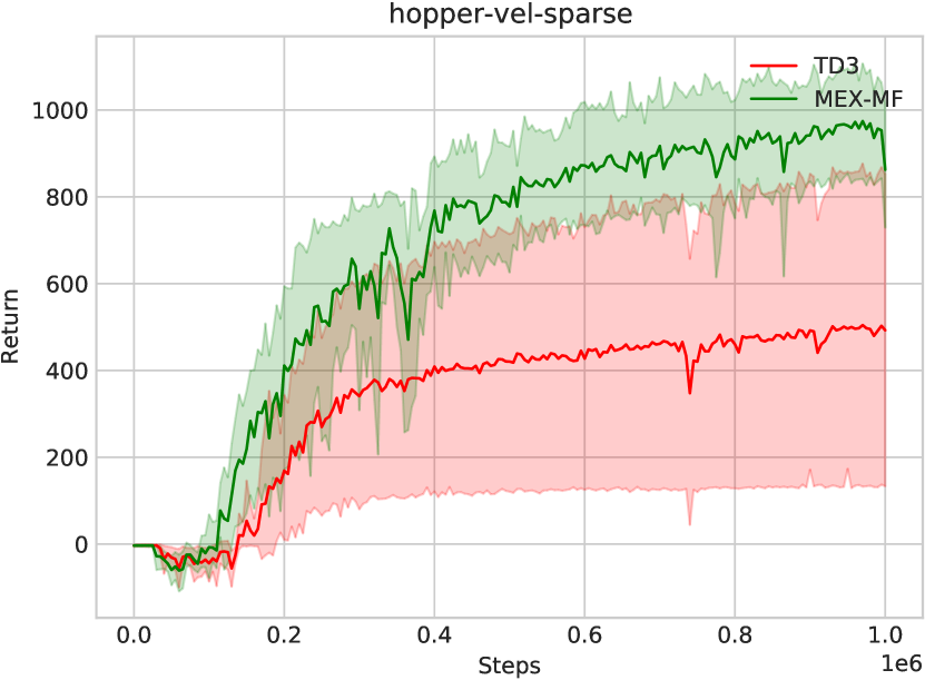
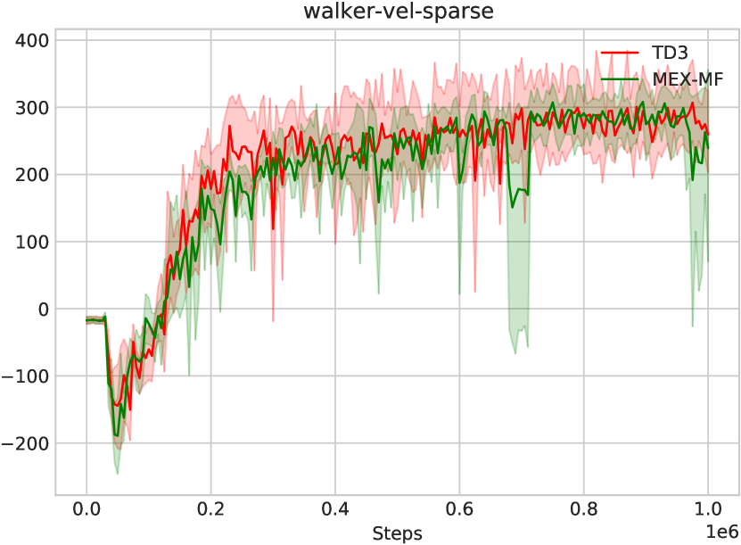
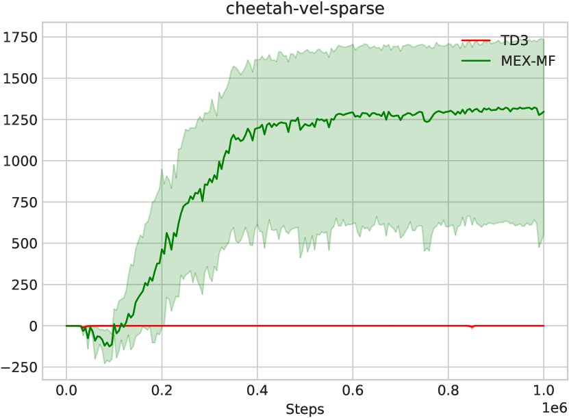
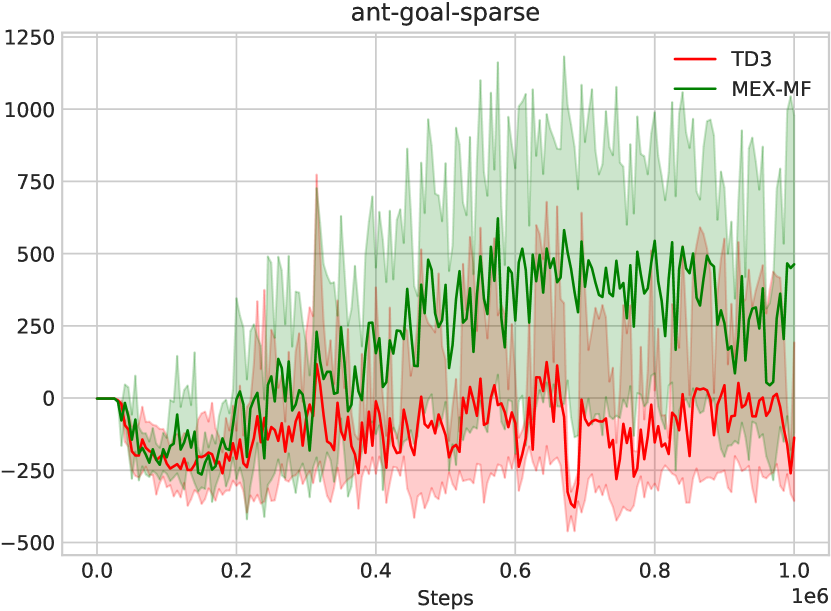
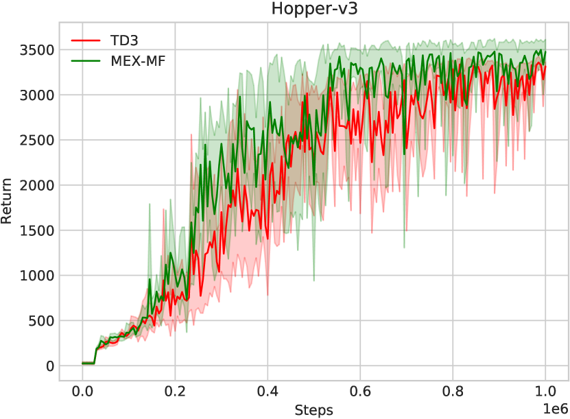
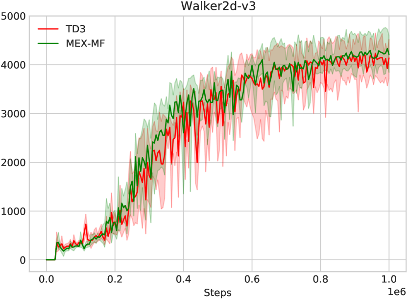
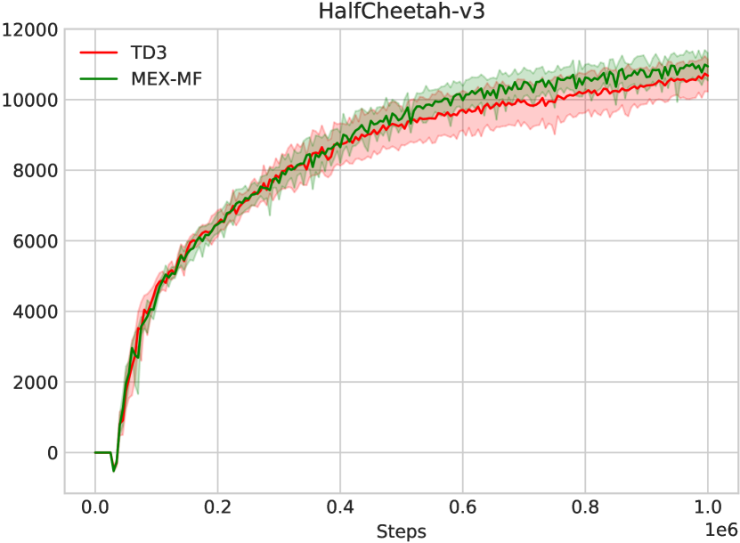
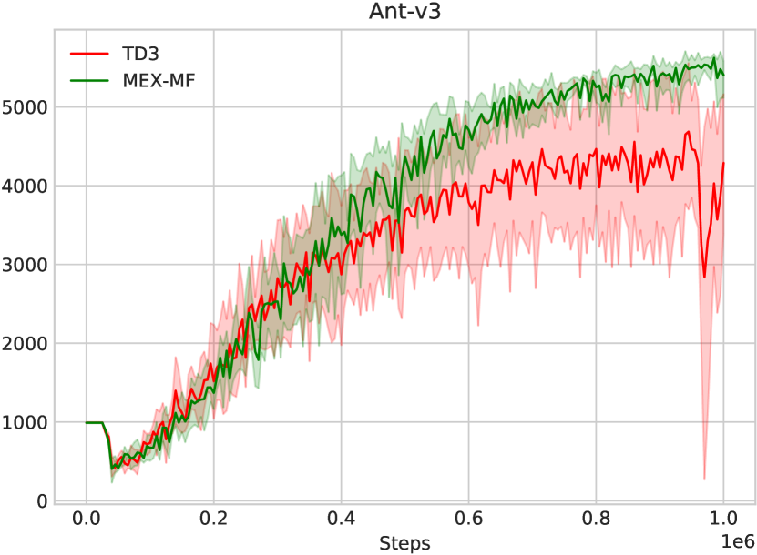
Figure 1: Model-free MEX-MF in sparse and standard MuJoCo locomotion tasks.

Results for MEX-MB.

We compare MEX-MB with MBPO (Janner et al., 2019), where our method differs from MBPO only in the inclusion of the value gradient in (7.3) during model updates. We find that MEX-MB offers an easy implementation with minimal computational overhead and yet remains highly effective across sparse and standard MuJoCo tasks. Notably, in the sparse reward settings, MEX-MB excels at achieving the goal velocity and outperforms MBPO by a stable margin. In standard gym tasks, MEX-MB showcases greater sample efficiency in challenging high-dimensional tasks with higher asymptotic returns.

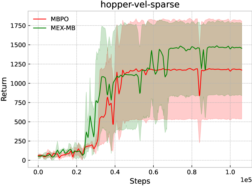
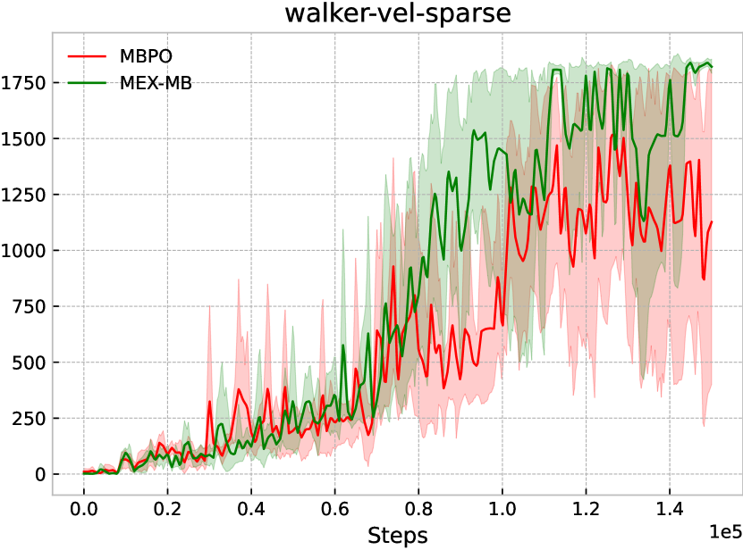
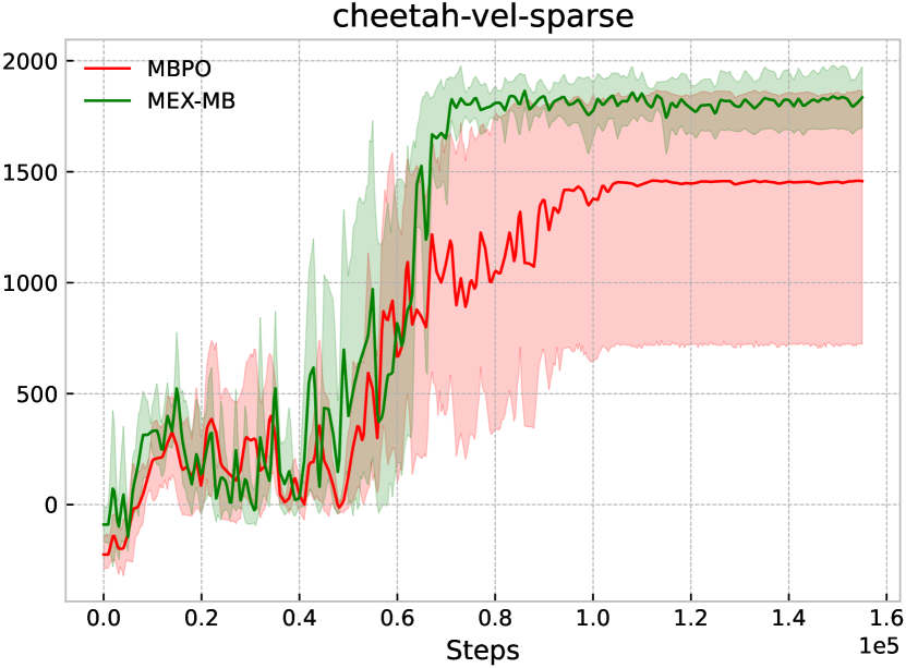
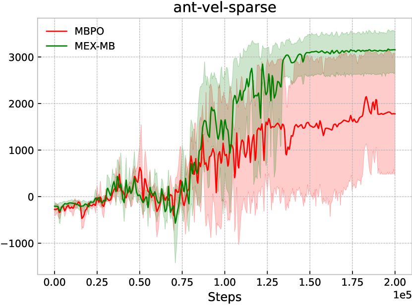
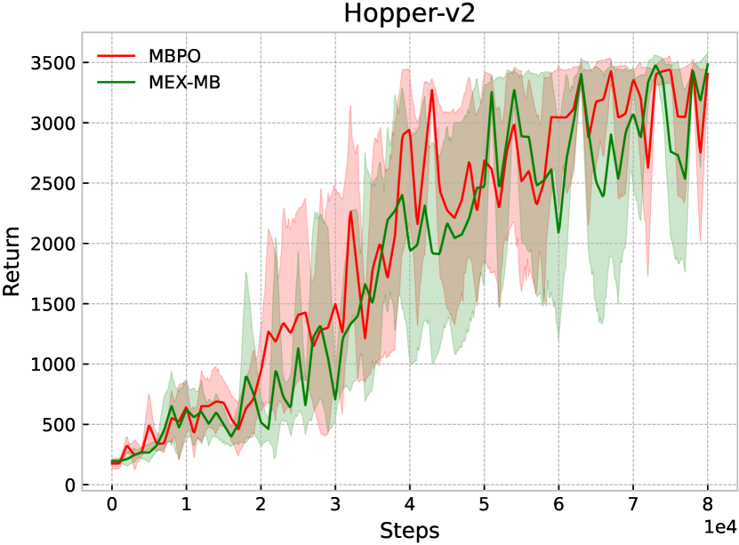
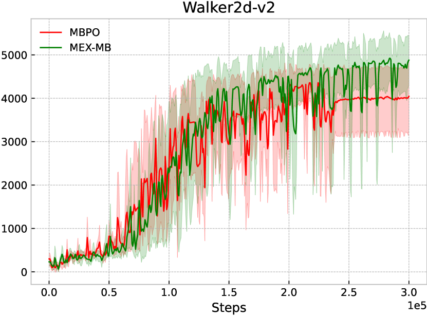
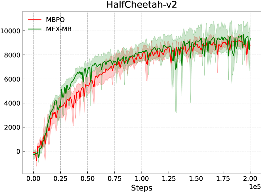
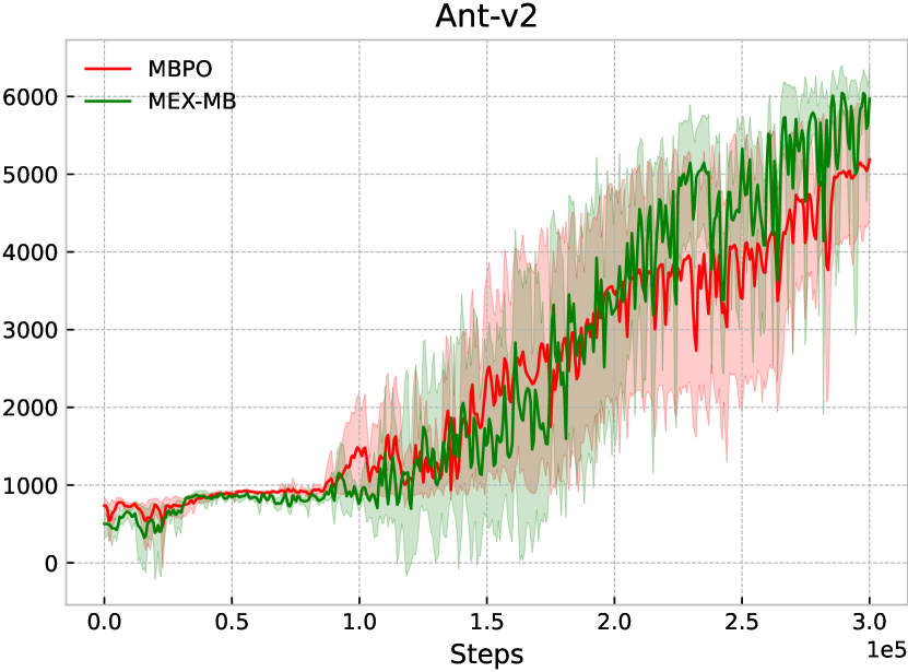
Figure 2: Model-based MEX-MB in sparse and standard MuJoCo locomotion tasks.

8 Conclusions

In this paper, we propose a novel online RL algorithm framework Maximize to Explore (MEX), aimed at striking a balance between exploration and exploitation in online learning scenarios. MEX is provably sample-efficient with general function approximations and is easy to implement. Theoretically, we prove that under mild structural assumptions (low generalized eluder coefficient (GEC)), MEX achieves $\widetilde{\mathcal{O}}(\sqrt{K})$-online regret for Markov decision processes. We further extend the definition of GEC and the MEX framework to two-player zero-sum Markov games and also prove the $\widetilde{\mathcal{O}}(\sqrt{K})$-online regret. In practice, we adapt MEX to deep RL methods in both model-based and model-free styles and apply them to sparse-reward MuJoCo environments, outperforming baselines significantly. We hope that our work can shed light on future research of designing both statistically efficient and practically effective RL algorithms with powerful function approximations.

Appendix A Proof of Main Theoretical Results

A.1 Proof of Theorem 4.4

Proof of Theorem 4.4.

Consider the following decomposition of the regret,

$$\mathrm{Regret}(K) =\sum_{k=1}^{K}V_{1}^{\ast}(x_{1})-V_{1}^{\pi_{f^{k}}}(x_{1})$$

$$=\underbrace{\sum_{k=1}^{K}V_{1}^{\ast}(x_{1})-V_{1,f^{k}}(x_{1})}_{\displaystyle{\text{Term (i)}}}+\underbrace{\sum_{k=1}^{K}V_{1,f^{k}}(x_{1})-V_{1}^{\pi_{f^{k}}}(x_{1})}_{\displaystyle{\text{Term (ii)}}}$$ (A.1)

Term (i).

Note that by our definition in both Example 2.2 and 2.1, we have that $V_{1}^{\ast}=V_{1,f^{\ast}}$. Thus we can rewrite the term (i) as

$$\text{Term (i)}=\sum_{k=1}^{K}V_{1,f^{\ast}}(x_{1})-V_{1,f^{k}}(x_{1}).$$ (A.2)

Then by our choice of $f^{k}$ in (3.1) and the fact that $f^{\ast}\in\mathcal{H}$, we have that for each $k\in[K]$,

$$V_{1,f^{\ast}}(x_{1})-\eta\sum_{h=1}^{H}L_{h}^{k-1}(f^{\ast})(x_{1})\leq V_{1,f^{k}}(x_{1})-\eta\sum_{h=1}^{H}L_{h}^{k-1}(f^{k})(x_{1})$$ (A.3)

By combining (A.2) and (A.3), we can derive that

$$\text{Term (i)}\leq\eta\sum_{k=1}^{K}\sum_{h=1}^{H}L_{h}^{k-1}(f^{\ast})-L_{h}^{k-1}(f^{k})$$ (A.4)

Now by applying Assumption 4.3 to (A.4), we can further derive that with probability at least $1-\delta$,

$$\text{Term (i)}\leq-c_{\mathrm{(i)}}\cdot\eta\sum_{k=1}^{K}\sum_{s=1}^{k-1}\sum_{h=1}^{H}\mathbb{E}_{\xi_{h}\sim\pi_{\mathrm{exp}}(f^{s})}[\ell_{f^{s}}(f^{k};\xi_{h})]+c_{\mathrm{(i)}}\cdot\eta BK\big{(}H\log(HK/\delta)+\log(|\mathcal{H}|)\big{)}.$$ (A.5)

where $c_{\mathrm{(i)}}>0$ is some absolute constant (recall the definition of $\lesssim$).

Term (ii).

For term (ii) of (A.2), we apply Assumption 4.2 and obtain that, for any $\epsilon>0$,

$$\text{Term (ii)}\leq\inf_{\mu>0}\left\{\frac{\mu}{2}\sum_{h=1}^{H}\sum_{k=1}^{K}\sum_{s=1}^{k-1}\mathbb{E}_{\xi_{h}\sim\pi_{\exp}(f^{s})}[\ell_{f^{s}}(f^{k};\xi_{h})]+\frac{d_{\mathrm{GEC}}(\epsilon)}{2\mu}+\sqrt{d_{\mathrm{GEC}}(\epsilon)HK}+\epsilon HK\right\}.$$

By taking $\mu/2=c_{\mathrm{(i)}}\cdot\eta$, we can further derive that,

$$\text{Term (ii)}\leq c_{\mathrm{(i)}}\cdot\eta\sum_{h=1}^{H}\sum_{k=1}^{K}\sum_{s=1}^{k-1}\mathbb{E}_{\xi_{h}\sim\pi_{\exp}(f^{s})}[\ell_{f^{s}}(f^{k};\xi_{h})]+\frac{d_{\mathrm{GEC}}(\epsilon)}{4c_{\mathrm{(i)}}\eta}+\sqrt{d_{\mathrm{GEC}}(\epsilon)HK}+\epsilon HK.$$ (A.6)

Combining Term (i) and Term (ii).

Now by combining (A.5) and (A.6), we can obtain that with probability at least $1-\delta$,

$$\mathrm{Regret}(T) =\text{Term (i)}+\text{Term (ii)}$$

$$\leq-c_{\mathrm{(i)}}\cdot\eta\sum_{k=1}^{K}\sum_{s=1}^{k-1}\sum_{h=1}^{H}\mathbb{E}_{\xi_{h}\sim\pi_{\mathrm{exp}}(f^{s})}[\ell_{f^{s}}(f^{k};\xi_{h})]+c_{\text{(i)}}\cdot\eta BK\big{(}H\log(HK/\delta)+\log(|\mathcal{H}|)\big{)},$$

$$\qquad+c_{\mathrm{(i)}}\cdot\eta\sum_{h=1}^{H}\sum_{k=1}^{K}\sum_{s=1}^{k-1}\mathbb{E}_{\xi_{h}\sim\pi_{\exp}(f^{s})}[\ell_{f^{s}}(f^{k};\xi_{h})]+\frac{d_{\mathrm{GEC}}(\epsilon)}{4c_{\mathrm{(i)}}\eta}+\sqrt{d_{\mathrm{GEC}}(\epsilon)HK}+\epsilon HK$$

$$=c_{\text{(i)}}\cdot\eta BK\big{(}H\log(HK/\delta)+\log(|\mathcal{H}|)\big{)}+\frac{d_{\mathrm{GEC}}(\epsilon)}{4c_{\mathrm{(i)}}\eta}+\sqrt{d_{\mathrm{GEC}}(\epsilon)HK}+\epsilon HK.$$ (A.7)

By taking $\epsilon=1/\sqrt{HK}$, $\eta=\sqrt{d_{\mathrm{GEC}}(\epsilon)/(H\log(HK/\delta)+\log(|\mathcal{H}|))\cdot B\cdot K)}$, we can derive from (A.7) that, with probability at least $1-\delta$, it holds that

$$\mathrm{Regret}(K)\lesssim\sqrt{d_{\mathrm{GEC}}(1/\sqrt{HK})\cdot(H\log(HK/\delta)+\log(|\mathcal{H}|))\cdot B\cdot K}.$$ (A.8)

This finishes the proof of Theorem 4.4. ∎

A.2 Proof of Theorem 6.7

Proof of Theorem 6.7.

Consider the following decomposition of the regret,

$$\mathrm{Regret}(K) =\sum_{k=1}^{K}V_{1}^{\ast}(x_{1})-V_{1}^{\mu^{k},\dagger}(x_{1})$$

$$=\sum_{k=1}^{K}V_{1}^{\ast}(x_{1})-V_{1}^{\mu^{k},\nu^{k}}(x_{1})+\sum_{k=1}^{K}V_{1}^{\mu^{k},\nu^{k}}(x_{1})-V_{1}^{\mu^{k},\dagger}(x_{1})$$

$$=\underbrace{\sum_{k=1}^{K}V_{1}^{\star}-V_{1,f^{k}}}_{\displaystyle{\text{Term (Max.i)}}}+\underbrace{\sum_{k=1}^{K}V_{1,f^{k}}-V_{1}^{\mu^{k},\nu^{k}}}_{\displaystyle{\text{Term (Max.ii)}}}+\underbrace{\sum_{k=1}^{K}V_{1,g^{k}}^{\mu^{k},\dagger}-V_{1}^{\mu^{k},\dagger}}_{\displaystyle{\text{Term (Min.i)}}}+\underbrace{\sum_{k=1}^{K}V_{1}^{\mu^{k},\nu^{k}}-V_{1,g^{k}}^{\mu^{k},\dagger}}_{\displaystyle{\text{Term (Min.ii)}}},$$ (A.9)

where in the last equality we omit the dependence on $x_{1}$ for simplicity.

Term (Max.i).

Note that by our definition in both Example 6.1 and Example 6.2, we have that $V_{1}^{\ast}=V_{1,f^{\ast}}$. Thus we can rewrite the term (Max.i) as

$$\text{Term (Max.i)}=\sum_{k=1}^{K}V_{1,f^{\ast}}(x_{1})-V_{1,f^{k}}(x_{1}).$$ (A.10)

Then by our choice of $f^{k}$ in (6.12) and the fact that $f^{\ast}\in\mathcal{H}$, we have that for each $k\in[K]$,

$$V_{1,f^{\ast}}(x_{1})-\eta\sum_{h=1}^{H}L_{h}^{k-1}(f^{\ast})\leq V_{1,f^{k}}(x_{1})-\eta\sum_{h=1}^{H}L_{h}^{k-1}(f^{k}).$$ (A.11)

By combining (A.10) and (A.11), we can derive that

$$\text{Term (Max.i)}\leq\eta\sum_{k=1}^{K}\sum_{h=1}^{H}L_{h}^{k-1}(f^{\ast})-L_{h}^{k-1}(f^{k}).$$ (A.12)

Now applying Assumption 6.6 to (A.12), we can further derive that with probability at least $1-\delta$,

$$\text{Term (Max.i)}\leq-c_{\mathrm{(max.i)}}\cdot\eta\sum_{k=1}^{K}\sum_{s=1}^{k-1}\sum_{h=1}^{H}\mathbb{E}_{\xi_{h}\sim\bm{\pi}^{k}}[\ell_{f^{s}}(f;\xi_{h})]+c_{\mathrm{(max.i)}}\cdot BK\big{(}H\log(HK/\delta)+\log(|\mathcal{H}|)\big{)},$$ (A.13)

for some absolute constant $c_{\mathrm{(max.i)}}>0$.

Term (Max.ii).

For term (Max.ii), we apply Assumption 6.5 and obtain that, for any $\epsilon>0$,

$$\text{Term (Max.ii)}\leq\inf_{\zeta>0}\left\{\frac{\zeta}{2}\sum_{h=1}^{H}\sum_{k=1}^{K}\sum_{s=1}^{k-1}\mathbb{E}_{\xi_{h}\sim\bm{\pi}^{k}}[\ell_{f^{s}}(f^{k};\xi_{h})]+\frac{d_{\mathrm{TGEC}}(\epsilon)}{2\zeta}+\sqrt{d_{\mathrm{TGEC}}(\epsilon)HK}+\epsilon HK\right\}.$$

By taking $\zeta/2=c_{\mathrm{(max.i)}}\cdot\eta$, we can further derive that

$$\text{Term (Max.ii)}\leq c_{\mathrm{(max.i)}}\cdot\eta\sum_{h=1}^{H}\sum_{k=1}^{K}\sum_{s=1}^{k-1}\mathbb{E}_{\xi_{h}\sim\bm{\pi}^{k}}[\ell_{f^{s}}(f^{k};\xi_{h})]+\frac{d_{\mathrm{TGEC}}(\epsilon)}{4c_{\mathrm{(max.i)}}\eta}+\sqrt{d_{\mathrm{TGEC}}(\epsilon)HK}+\epsilon HK.$$ (A.14)

Term (Min.i).

For either model-free or model-based hypothsis, by our definition in Example 6.1 and Example 6.2 respectively, we both have that $V_{1}^{\mu^{k},\dagger}=V_{1,\star}^{\mu^{k},\dagger}$. Here $\star=Q^{\mu^{k},\dagger}$ for model-free hypothesis and $\star=f^{\ast}$ for model-based hypothesis. Thus we can rewrite the term (Min.i) as.

$$\text{Term (Min.i)}=\sum_{k=1}^{K}V_{1,g^{k}}^{\mu^{k},\dagger}(x_{1})-V_{1,\star}^{\mu^{k},\dagger}(x_{1}).$$ (A.15)

Then by our choice of $g^{k}$ in (6.13) and the fact that $\star\in\mathcal{H}$ (Assumption 6.3), we have that for each $k\in[K]$,

$$-V_{1,\star}^{\mu^{k},\dagger}(x_{1})-\eta\sum_{h=1}^{H}L_{h,\mu^{k}}^{k-1}(\star)\leq-V_{1,g^{k}}^{\mu^{k},\dagger}(x_{1})-\eta\sum_{h=1}^{H}L_{h,\mu^{k}}^{k-1}(g^{k})$$ (A.16)

By combining (A.15) and (A.16), we can derive that

$$\text{Term (Min.i)}\leq\eta\sum_{k=1}^{K}\sum_{h=1}^{H}L_{h,\mu^{k}}^{k-1}(\star)-L_{h,\mu^{k}}^{k-1}(g^{k})$$ (A.17)

Now applying Assumption 6.6 to (A.17), we can further derive that with probability at least $1-\delta$,

$$\text{Term (Min.i)}\leq-c_{\mathrm{(min.i)}}\cdot\eta\sum_{k=1}^{K}\sum_{s=1}^{k-1}\sum_{h=1}^{H}\mathbb{E}_{\xi_{h}\sim\bm{\pi}^{k}}[\ell_{g^{s},\mu^{k}}(g;\xi_{h})]+c_{\mathrm{(min.i)}}\cdot\eta BK\big{(}H\log(HK/\delta)+\log(|\mathcal{H}|)\big{)}.$$ (A.18)

Term (Min.ii).

For term (Min.ii), we apply Assumption 6.5 and obtain that, for any $\epsilon>0$,

$$\text{Term (Min.ii)}\leq\inf_{\zeta>0}\left\{\frac{\zeta}{2}\sum_{h=1}^{H}\sum_{k=1}^{K}\sum_{s=1}^{k-1}\mathbb{E}_{\xi_{h}\sim\bm{\pi}^{k}}[\ell_{g^{s},\mu^{k}}(g^{k};\xi_{h})]+\frac{d_{\mathrm{TGEC}}(\epsilon)}{2\zeta}+\sqrt{d_{\mathrm{TGEC}}(\epsilon)HK}+\epsilon HK\right\}.$$

By taking $\zeta/2=c_{\mathrm{(min.i)}}\cdot\eta$, we can further derive that

$$\!\!\!\!\!\!\text{Term (Max.ii)}\leq c_{\mathrm{(min.i)}}\cdot\eta\sum_{h=1}^{H}\sum_{k=1}^{K}\sum_{s=1}^{k-1}\mathbb{E}_{\xi_{h}\sim\bm{\pi}^{k}}[\ell_{g^{s},\mu^{k}}(g^{k};\xi_{h})]+\frac{d_{\mathrm{TGEC}}(\epsilon)}{4c_{\mathrm{(min.i)}}\eta}+\sqrt{d_{\mathrm{TGEC}}(\epsilon)HK}+\epsilon HK.$$ (A.19)

Combining Term (Max.i), Term (Max.ii), Term (Min.i), and Term (Min.ii).

Finally, combining (A.13), (A.14), (A.18), and (A.14), taking $\epsilon=1/\sqrt{HK}$ and

$$\eta=\sqrt{\frac{d_{\mathrm{TGEC}}(1/\sqrt{HK})}{(H\log(HK/\delta)+\log(|\mathcal{H}|))\cdot B\cdot K}},$$ (A.20)

we can finally derive that with probability at least $1-2\delta$,

$$\mathrm{Regret}(K)\lesssim\sqrt{d_{\mathrm{TGEC}}(1/\sqrt{HK})\cdot(H\log(HK/\delta)+\log(|\mathcal{H}|))\cdot B\cdot K}.$$

This finishes the proof of Theorem 6.7. ∎

Appendix B Examples of Model-based and Model-free Online RL in MDPs

In this section, we specify Corollaries 5.2 and 5.4 to various examples of MDPs with low generalized eluder coefficient (GEC Zhong et al. (2022)). Sections B.1 and B.2 consider model-free hypothesis and model-based hypothesis, respectively. After, we give proof of the generalization guarantees involved in Section 5. Section B.3 provides proof of Proposition 5.1 and Section B.4 provides proof of Proposition 5.3.

B.1 Examples of Model-free Online RL in MDPs

MDPs with low Bellman eluder dimension.

In this part, we study MDPs with low Bellman eluder (BE) dimension (Jin et al., 2021a). To introduce, we define the notion of $\epsilon$-independence between distributions and the notion of distributional eluder dimension.

Definition B.1 ($\epsilon$-independence between distributions).

Let $\mathcal{G}$ be a function class on the space $\mathcal{X}$, and let $\nu,\mu_{1},\cdots,\mu_{n}$ be probability measures on $\mathcal{X}$. We say $\nu$ is $\epsilon$-independent of $\{\mu_{1},\cdots,\mu_{n}\}$ with respect to $\mathcal{G}$ if there exists a $g\in\mathcal{G}$ such that $\sqrt{\sum_{i=1}^{n}(\mathbb{E}_{\mu_{i}}[g])^{2}}\leq\epsilon$ but $|\mathbb{E}_{\nu}[g]|>\epsilon$.

Definition B.2 (Distributional Eluder (DE) dimension).

Let $\mathcal{G}$ be a function class on space $\mathcal{X}$, and let $\Pi$ be a family of probability measures on $\mathcal{X}$. The distributional eluder dimension $\operatorname{dim}_{\mathrm{DE}}(\mathcal{G},\Pi,\epsilon)$ is defined as the length of the longest sequence $\{\rho_{1},\cdots,\rho_{n}\}\subset\Pi$ such that there exists $\epsilon^{\prime}\geq\epsilon$ with $\rho_{i}$ being $\epsilon^{\prime}$-independent of $\{\rho_{1},\cdots,\rho_{i-1}\}$ for each $i\in[n]$.

The Bellman eluder dimension is based upon the notion of distributional eluder dimsntion. For a model-free hypothesis class $\mathcal{H}$, we the Bellman operator $\mathcal{T}_{h}$ defined in Section 2 becomes,

$$(\mathcal{T}_{h}f_{h+1})(x,a)=R_{h}(x,a)+\mathbb{E}_{x^{\prime}\sim\mathbb{P}_{h}(\cdot|x,a)}[V_{h+1,f}(x^{\prime})],$$ (B.1)

for any $f\in\mathcal{H}$. Then we define the $Q$-type/$V$-type Bellman eluder dimension as the following.

Definition B.3 ($Q$-type Bellman eluder (BE) dimension (Jin et al., 2021a; Zhong et al., 2022)).

We define $(I-\mathcal{T}_{h})\mathcal{H}=\{(x,a)\mapsto(f_{h}-\mathcal{T}_{h}f_{h+1})(x,a):f\in\mathcal{H}\}$ as the set of Bellman residuals induced by $\mathcal{H}$ at step $h$, and let $\Pi=\{\Pi_{h}\}_{h=1}^{H}$ be a collection of $H$ families of probability measure over $\mathcal{S}\times\mathcal{A}$. The $Q$-type $\epsilon$-Bellman eluder dimension of $\mathcal{H}$ with respect to $\Pi$ is defined as

$$\operatorname{dim}_{\mathrm{BE}}(\mathcal{H},\Pi,\epsilon)=\max_{h\in[H]}\left\{\operatorname{dim}_{\mathrm{DE}}\left(\left(I-\mathcal{T}_{h}\right)\mathcal{H},\Pi_{h},\epsilon\right)\right\}.$$

Definition B.4 ($V$-type Bellman eluder (BE) dimension (Jin et al., 2021a; Zhong et al., 2022)).

We define $(I-\mathcal{T}_{h})V_{\mathcal{H}}=\{x\mapsto(f_{h}-\mathcal{T}_{h}f_{h+1})(x,\pi_{h,f}(x)):f\in\mathcal{H}\}$ as the set of $V$-type Bellman residuals induced by $\mathcal{H}$ at step $h$, and let $\Pi=\{\Pi_{h}\}_{h=1}^{H}$ be a collection of $H$ families of probability measure over $\mathcal{S}$. The $V$-type $\epsilon$-Bellman eluder dimension of $\mathcal{H}$ with respect to $\Pi$ is defined as

$$\operatorname{dim}_{\mathrm{VBE}}(\mathcal{H},\Pi,\epsilon)=\max_{h\in[H]}\left\{\operatorname{dim}_{\mathrm{DE}}\left(\left(I-\mathcal{T}_{h}\right)V_{\mathcal{H}},\Pi_{h},\epsilon\right)\right\}.$$

For MDPs with low Bellman eluder dimension, we choose the function $l$ in Assumption 3.1 as

$$l_{f^{\prime}}\big{(}(f_{h},f_{h+1});\mathcal{D}_{h}\big{)}=Q_{h,f}(x_{h},a_{h})-r_{h}-V_{h+1,f}(x_{h+1}).$$ (B.2)

and we choose the operator $\mathcal{P}_{h}=\mathcal{T}_{h}$ defined in (B.1). One can check that such a choice satisfies Assumption 3.1. By further choosing the exploration policy as $\pi_{\mathrm{exp}}(f)=\pi_{f}$ for $Q$-type problems and $\pi_{\exp}(f)=\pi_{f}\circ_{h}\mathrm{Unif}(\mathcal{A})$ for $V$-type problems, we can bound the GEC for MDPs with low BE dimension by the following lemma.

Lemma B.5 (GEC for low Bellman eluder dimension, Lemma 3.16 in Zhong et al. (2022)).

Let the discrepancy $\ell$ function be chosen as (5.1) with $l$ defined in (B.2). Define $\Pi_{\mathcal{H}}$ as the distributions induced by following some $f\in\mathcal{H}$ greedily. For $Q$-type problems, by choosing $\pi_{\mathrm{exp}}(f)=\pi_{f}$, we have that

$$d_{\mathrm{GEC}}(\epsilon)\leq 2\operatorname{dim}_{\mathrm{BE}}(\mathcal{H},\Pi_{\mathcal{H}},\epsilon)H\cdot\log(K),$$

For $V$-type problems, by choosing $\pi_{\exp}(f)=\pi_{f}\circ_{h}\mathrm{Unif}(\mathcal{A})$, we have that

$$d_{\mathrm{GEC}}(\epsilon)\leq 2\operatorname{dim}_{\mathrm{VBE}}(\mathcal{H},\Pi_{\mathcal{H}},\epsilon)|\mathcal{A}|H\cdot\log(K).$$

Proof of Lemma B.5.

See Lemma 3.16 in Zhong et al. (2022) for a detailed proof. ∎

By combining Lemma B.5 and Corollary 5.2, we can obtain that for $Q$-type low Bellman eluder dimension problem, it holds that with probability at least $1-\delta$,

$$\mathrm{Regret}(T)\lesssim B_{l}^{2}\cdot\sqrt{\operatorname{dim}_{\mathrm{BE}}(\mathcal{H},\Pi_{\mathcal{H}},1/\sqrt{HK})\cdot\log(HK|\mathcal{H}|/\delta)\cdot H^{2}K},$$ (B.3)

and for $V$-type Bellman eluder dimension problem, it holds that with probability at least $1-\delta$,

$$\mathrm{Regret}(T)\lesssim B_{l}^{2}\cdot\sqrt{\operatorname{dim}_{\mathrm{VBE}}(\mathcal{H},\Pi_{\mathcal{H}},1/\sqrt{HK})\cdot|\mathcal{A}|\cdot\log(HK|\mathcal{H}|/\delta)\cdot H^{2}K}.$$ (B.4)

MDPs of bilinear class.

In this part, we consider MDPs of bilinear class (Du et al., 2021).

Definition B.6 (Bilinear class (Du et al., 2021; Zhong et al., 2022)).

Given an MDP, a model-free hypothesis class $\mathcal{H}$, and a function $l_{f}:\mathcal{H}\times\mathcal{H}\times(\mathcal{S}\times\mathcal{A}\times\mathbb{R}\times\mathcal{S})\mapsto\mathbb{R}$, we say the corresponding RL problem is in a bilinear class if there exist functions $W_{h}:\mathcal{H}\mapsto\mathcal{V}$ and $X_{h}:\mathcal{H}\mapsto\mathcal{V}$ for some Hilbert space $\mathcal{V}$, such that for all $f,g\in\mathcal{H}$ and $h\in[H]$, we have that

$$\left|\mathbb{E}_{\pi_{f}}[Q_{h,f}(x_{h},a_{h})-R_{h}(x_{h},a_{h})-V_{h+1,f}(x_{h+1})]\right| \leq\left|\langle W_{h}(f)-W_{h}(f^{\ast}),X_{h}(f)\rangle_{\mathcal{V}}\right|,$$

$$\left|\mathbb{E}_{x_{h}\sim\pi_{f},a_{h}\sim\widetilde{\pi}}[l_{f}(g;\xi_{h})]\right| =\left|\langle W_{h}(g)-W_{h}(f^{\ast}),X_{h}(f)\rangle_{\mathcal{V}}\right|,$$

where $\widetilde{\pi}$ is either $\pi_{f}$ for $Q$-type problems or $\pi_{g}$ for $V$-type problems. Meanwhile, we make the assumption that $\sup_{f\in\mathcal{H},h\in[H]}\|W_{h}(f)\|_{2}\leq 1$ and $\sup_{f\in\mathcal{H},h\in[H]}\|X_{h}(f)\|_{2}\leq 1$.

For MDPs of bilinear class, we choose the function $l$ as the function introduced in the definition of bilinear class. By choosing the exploration policy as $\pi_{\mathrm{exp}}(f)=\pi_{f}$ for $Q$-type problems and $\pi_{\exp}(f)=\pi_{f}\circ_{h}\mathrm{Unif}(\mathcal{A})$ for $V$-type problems, we can bound the generalized eluder coefficient for MDPs of bilinear class using the following lemma. To simplify the notation, we define $\mathcal{X}_{h}=\{X_{h}(f):f\in\mathcal{H}\}\subseteq\mathcal{V}$ and $\mathcal{X}=\{\mathcal{X}_{h}:h\in[H]\}$.

Lemma B.7 (GEC for bilinear class, Lemma 3.22 in Zhong et al. (2022)).

Let the discrepancy $\ell$ function be chosen as (5.1) with $l$ defined in Definition B.6. Define the maximum information gain $\gamma_{K}(\epsilon,\mathcal{X})$ as

$$\gamma_{K}(\epsilon,\mathcal{X})=\sum_{h=1}^{H}\max_{x_{1},\cdots,x_{K}\in\mathcal{X}_{h}}\log\operatorname{det}\Bigg{(}\mathcal{I}(\cdot)+\frac{1}{\epsilon}\sum_{s=1}^{K}x_{s}\langle x_{s},\cdot\rangle_{\mathcal{V}}\Bigg{)}$$

with $\mathcal{I}$ being the identity mapping. Then for $Q$-type problems, choosing $\pi_{\mathrm{exp}}(f)=\pi_{f}$, we have that

$$d_{\mathrm{GEC}}(\epsilon)\leq 2\gamma_{K}(\epsilon,\mathcal{X}).$$

For $V$-type problems, by choosing $\pi_{\exp}(f)=\pi_{f}\circ_{h}\mathrm{Unif}(\mathcal{A})$, we have that

$$d_{\mathrm{GEC}}(\epsilon)\leq 2|\mathcal{A}|\gamma_{K}(\epsilon,\mathcal{X}).$$

Proof of Lemma B.5.

See Lemma 3.22 in Zhong et al. (2022) for a detailed proof. ∎

By combining Lemma B.7 and Corollary 5.2, we know that For $Q$-type bilinear class problem, it holds that with probability at least $1-\delta$,

$$\mathrm{Regret}(T)\lesssim\sqrt{\gamma_{K}(1/\sqrt{HK},\mathcal{X})\cdot\log(HK|\mathcal{H}|/\delta)\cdot HK},$$ (B.5)

and for $V$-type bilinear class problem, it holds that with probability at least $1-\delta$,

$$\mathrm{Regret}(T)\lesssim\sqrt{\gamma_{K}(1/\sqrt{HK},\mathcal{X})\cdot|\mathcal{A}|\cdot\log(HK|\mathcal{H}|/\delta)\cdot HK}.$$ (B.6)

B.2 Examples of Model-based Online RL in MDPs

MDPs with low witness rank. We consider the example of MDPs with low witness rank (Sun et al., 2019; Agarwal and Zhang, 2022). To introduce, we define the function class $\mathcal{V}=\{\upsilon:\mathcal{S}\times\mathcal{A}\times\mathcal{S}\mapsto[0,1]\}$.

Definition B.8 (Q-type/V-type witness rank (Sun et al., 2019; Agarwal and Zhang, 2022)).

An MDP is called of witness rank $d$ if for any two models $f,f^{\prime}\in\mathcal{H}$, there exists mappings $X_{h}:\mathcal{H}\mapsto\mathbb{R}^{d}$ and $W_{h}:\mathcal{H}\mapsto\mathbb{R}^{d}$ for each timestep $h$ such that,

$$\max_{\upsilon\in\mathcal{V}}\mathbb{E}_{x_{h}\sim\pi_{f},a_{h}\sim\widetilde{\pi}}\left[\left(\mathbb{E}_{x^{\prime}\sim\mathbb{P}_{h,f^{\prime}}(\cdot|x_{h},a_{h})}-\mathbb{E}_{x^{\prime}\sim\mathbb{P}_{h,f^{\ast}}(\cdot|x_{h},a_{h})}\right)[\upsilon(x_{h},a_{h},x^{\prime})]\right] \geq\langle W_{h}(f^{\prime}),X_{h}(f)\rangle,$$

$$\kappa_{\mathrm{wit}}\cdot\mathbb{E}_{x_{h}\sim\pi_{f},a_{h}\sim\widetilde{\pi}}\left[\left(\mathbb{E}_{x^{\prime}\sim\mathbb{P}_{h,f^{\prime}}(\cdot|x_{h},a_{h})}-\mathbb{E}_{x^{\prime}\sim\mathbb{P}_{h,f^{\ast}}(\cdot|x_{h},a_{h})}\right)[V_{h+1,f^{\prime}}(x^{\prime})]\right] \leq\langle W_{h}(f^{\prime}),X_{h}(f)\rangle,$$

where $\widetilde{\pi}$ is either $\pi_{f}$ for $Q$-type problems or $\pi_{f^{\prime}}$ for $V$-type problems and $\kappa_{\mathrm{wit}}\in(0,1]$ is a constant. Also, we let $\sup_{f\in\mathcal{H},h\in[H]}\|W_{h}(f)\|\leq 1$ and $\sup_{f\in\mathcal{H},h\in[H]}\|X_{h}(f)\|\leq 1$.

By choosing the exploration policy as $\pi_{\mathrm{exp}}(f)=\pi_{f}$ for $Q$-type problems and $\pi_{\exp}(f)=\pi_{f}\circ_{h}\mathrm{Unif}(\mathcal{A})$ for $V$-type problems, we can bound the generalized eluder coefficient by the following lemma.

Lemma B.9 (GEC for low witness rank, Lemma 3.22 in Zhong et al. (2022)).

Let the discrepancy function $\ell$ be chosen as (5.4). For $Q$-type problems, by choosing $\pi_{\mathrm{exp}}(f)=\pi_{f}$, we have that

$$d_{\mathrm{GEC}}(\epsilon)\leq 4dH\cdot\log(1+K/(\epsilon\kappa^{2}_{\mathrm{wit}}))/\kappa^{2}_{\mathrm{wit}}.$$

For $V$-type problems, by choosing $\pi_{\exp}(f)=\pi_{f}\circ_{h}\mathrm{Unif}(\mathcal{A})$, we have that

$$d_{\mathrm{GEC}}(\epsilon)\leq 4d|\mathcal{A}|H\cdot\log(1+K/(\epsilon\kappa^{2}_{\mathrm{wit}}))/\kappa^{2}_{\mathrm{wit}}.$$

Proof of Lemma B.9.

See Lemma 3.22 in Zhong et al. (2022) for a detailed proof. ∎

By combining Lemma B.9 and Corollary 5.4, we know that For $Q$-type low witness rank problem, it holds that with probability at least $1-\delta$,

$$\mathrm{Regret}(K)\lesssim\sqrt{4dH^{2}K\cdot\log(H|\mathcal{H}|/\delta)\cdot\log(1+H^{1/2}K^{3/2}/\kappa^{2}_{\mathrm{wit}})/\kappa^{2}_{\mathrm{wit}}},$$ (B.7)

and for $V$-type low witness rank problem, it holds that with probability at least $1-\delta$,

$$\mathrm{Regret}(K)\lesssim\sqrt{4d|\mathcal{A}|H^{2}K\cdot\log(H|\mathcal{H}|/\delta)\cdot\log(1+H^{1/2}K^{3/2}/\kappa^{2}_{\mathrm{wit}})/\kappa^{2}_{\mathrm{wit}}}.$$ (B.8)

B.3 Proof of Proposition 5.1

Proof of Proposition 5.1.

To prove Proposition 5.1, we define the random variables $X_{h,f}^{k}$ as

$$X_{h,f}^{k}=l_{f^{k}}((f_{h},f_{h+1});\mathcal{D}_{h}^{k})^{2}-l_{f^{k}}((\mathcal{P}_{h}f_{h+1},f_{h+1});\mathcal{D}_{h}^{k})^{2},$$ (B.9)

for any $f\in\mathcal{H}$, where the operator $\mathcal{P}_{h}$ is introduced in Assumption 3.1. We first show that $X_{h,f}^{k}$ is an unbiased estimator of the discrepancy function $\ell_{f^{k}}(f)$. Consider that

$$l_{f^{k}}((f_{h},f_{h+1});\mathcal{D}_{h}^{k})^{2} =\left(l_{f^{k}}((f_{h},f_{h+1});\mathcal{D}_{h}^{k})-l_{f^{k}}((\mathcal{P}_{h}f_{h+1},f_{h+1});\mathcal{D}_{h}^{k})+l_{f^{k}}((\mathcal{P}_{h}f_{h+1},f_{h+1});\mathcal{D}_{h}^{k})\right)^{2}$$

$$=\left(\mathbb{E}_{x_{h+1}^{k}\sim\mathbb{P}_{h}(\cdot|x_{h}^{k},a_{h}^{k})}[l_{f^{k}}((f_{h},f_{h+1});\mathcal{D}_{h}^{k})]+l_{f^{k}}((\mathcal{P}_{h}f_{h+1},f_{h+1});\mathcal{D}_{h}^{k})\right)^{2}$$

$$=\left(\mathbb{E}_{x_{h+1}^{k}\sim\mathbb{P}_{h}(\cdot|x_{h}^{k},a_{h}^{k})}[l_{f^{k}}((f_{h},f_{h+1});\mathcal{D}_{h}^{k})]\right)^{2}+l_{f^{k}}((\mathcal{P}_{h}f_{h+1},f_{h+1});\mathcal{D}_{h}^{k})^{2}$$

$$\qquad+2\mathbb{E}_{x_{h+1}^{k}\sim\mathbb{P}_{h}(\cdot|x_{h}^{k},a_{h}^{k})}[l_{f^{k}}((f_{h},f_{h+1});\mathcal{D}_{h}^{k})]\cdot l_{f^{k}}((\mathcal{P}_{h}f_{h+1},f_{h+1});\mathcal{D}_{h}^{k}),$$ (B.10)

where in the second equality we apply the generalized Bellman completeness condition in Assumption 3.1. By the generalized Bellman completeness condition again, we also have that in (B.10),

$$\mathbb{E}_{x^{k}_{h+1}\sim\mathbb{P}_{h}(\cdot|x_{h}^{k},a_{h}^{k})}\left[\mathbb{E}_{x_{h+1}^{k}\sim\mathbb{P}_{h}(\cdot|x_{h}^{k},a_{h}^{k})}[l_{f^{k}}((f_{h},f_{h+1});\mathcal{D}_{h}^{k})]\cdot l_{f^{k}}((\mathcal{P}_{h}f_{h+1},f_{h+1});\mathcal{D}_{h}^{k})\right]$$

$$\qquad=\mathbb{E}_{x_{h+1}^{k}\sim\mathbb{P}_{h}(\cdot|x_{h}^{k},a_{h}^{k})}[l_{f^{k}}((f_{h},f_{h+1});\mathcal{D}_{h}^{k})]\cdot\mathbb{E}_{x_{h+1}^{k}\sim\mathbb{P}_{h}(\cdot|x_{h}^{k},a_{h}^{k})}[l_{f^{k}}((\mathcal{P}_{h}f_{h+1},f_{h+1});\mathcal{D}_{h}^{k})]$$

$$\qquad=\mathbb{E}_{x_{h+1}^{k}\sim\mathbb{P}_{h}(\cdot|x_{h}^{k},a_{h}^{k})}[l_{f^{k}}((f_{h},f_{h+1});\mathcal{D}_{h}^{k})]$$

$$\qquad\qquad\cdot\mathbb{E}_{x_{h+1}^{k}\sim\mathbb{P}_{h}(\cdot|x_{h}^{k},a_{h}^{k})}\left[l_{f^{k}}((f_{h},f_{h+1});\mathcal{D}_{h}^{k})-\mathbb{E}_{x_{h+1}^{k}\sim\mathbb{P}_{h}(\cdot|x_{h}^{k},a_{h}^{k})}[l_{f^{k}}((f_{h},f_{h+1});\mathcal{D}_{h}^{k})]\right]$$

$$\qquad=0.$$ (B.11)

Thus by combining (B.10) and (B.11), we can derive that

$$\mathbb{E}_{x^{k}_{h+1}\sim\mathbb{P}_{h}(\cdot|x_{h}^{k},a_{h}^{k})}[X_{h,f}^{k}]=\left(\mathbb{E}_{x_{h+1}^{k}\sim\mathbb{P}_{h}(\cdot|x_{h}^{k},a_{h}^{k})}[l_{f^{k}}((f_{h},f_{h+1});\mathcal{D}_{h}^{k})]\right)^{2}=\ell_{f^{k}}(f;\mathcal{D}_{h}^{k}),$$ (B.12)

Now for each timestep $h$, we define a filtration $\{\mathcal{F}_{h,k}\}_{k=1}^{K}$, with

$$\mathcal{F}_{h,k}=\sigma\left(\bigcup_{s=1}^{k}\bigcup_{h=1}^{H}\mathcal{D}_{h}^{s}\right),$$ (B.13)

where $\mathcal{D}_{h}^{s}=\{x_{h}^{s},a_{h}^{s},r_{h}^{s},x_{h+1}^{s}\}$. From previous arguments, we can derive that

$$\mathbb{E}[X_{h,f}^{k}|\mathcal{F}_{h,k-1}]=\mathbb{E}\left[\mathbb{E}_{x^{k}_{h+1}\sim\mathbb{P}_{h}(\cdot|x_{h}^{k},a_{h}^{k})}[X_{h,f^{k}}]\middle|\mathcal{F}_{h,k-1}\right]=\mathbb{E}_{\xi_{h}\sim\pi_{\exp}(f^{k})}[\ell_{f^{k}}(f;\xi_{h})].$$ (B.14)

and that

$$\mathbb{V}[X_{h,f}^{k}|\mathcal{F}_{h,k-1}]\leq\mathbb{E}[(X_{h,f}^{k})^{2}|\mathcal{F}_{h,k-1}]\leq 4B_{l}^{2}\mathbb{E}[X_{h,f}^{k}|\mathcal{F}_{h,k-1}]=4B_{l}^{2}\mathbb{E}_{\xi_{h}\sim\pi_{\exp}(f^{k})}[\ell_{f^{k}}(f;\xi_{h})],$$ (B.15)

where $B_{l}$ is the upper bound of $l$ defined in Assumption 3.1. By applying Lemma D.2, (B.14), and (B.15), we can obtain that with probability at least $1-\delta$, for any $(h,k)\in[H]\times[K]$, $(f_{h},f_{h+1})\in\mathcal{H}_{h}\times\mathcal{H}_{h+1}$,

$$\left|\sum_{s=1}^{k-1}\mathbb{E}_{\xi_{h}\sim\pi_{\exp}(f^{s})}[\ell_{f^{s}}(f;\xi_{h})]-\sum_{s=1}^{k-1}X_{h,f}^{s}\right|\lesssim\frac{1}{2}\sum_{s=1}^{k-1}\mathbb{E}_{\xi_{h}\sim\pi_{\exp}(f^{s})}[\ell_{f^{s}}(f;\xi_{h})]+8B_{l}^{2}\log(HK|\mathcal{H}_{h}||\mathcal{H}_{h+1}|/\delta).$$ (B.16)

Rearranging terms in (B.16), we can further obtain that

$$-\sum_{s=1}^{k-1}X_{h,f}^{s}\lesssim-\frac{1}{2}\sum_{s=1}^{k-1}\mathbb{E}_{\xi_{h}\sim\pi_{\exp}(f^{s})}[\ell_{f^{s}}(f;\xi_{h})]+8B_{l}^{2}\log(HK|\mathcal{H}_{h}||\mathcal{H}_{h+1}|/\delta).$$ (B.17)

Meanwhile, by the definition of $X_{h,f}^{k}$ in (B.9) and the loss function $L$ in (3.3), we have that

$$\sum_{s=1}^{k-1}X_{h,f}^{s} =\sum_{s=1}^{k-1}l_{f^{s}}((f_{h},f_{h+1}),\mathcal{D}_{h}^{s})^{2}-\sum_{s=1}^{k-1}l_{f^{k}}((\mathcal{P}_{h}f_{h+1},f_{h+1}),\mathcal{D}_{h}^{s})^{2}$$

$$\leq\sum_{s=1}^{k-1}l_{f^{s}}((f_{h},f_{h+1}),\mathcal{D}_{h}^{s})^{2}-\inf_{f^{\prime}_{h}\in\mathcal{F}}\sum_{s=1}^{k-1}l_{f^{s}}((f^{\prime}_{h},f_{h+1}),\mathcal{D}_{h}^{s})^{2}$$

$$=L_{h}^{k-1}(f).$$ (B.18)

Thus by (B.17) and (B.3), we can derive that with probability at least $1-\delta$, for any $f\in\mathcal{H}$, $k\in[K]$,

$$-\sum_{h=1}^{H}L_{h}^{k-1}(f)\lesssim-\frac{1}{2}\sum_{h=1}^{H}\sum_{s=1}^{k-1}\mathbb{E}_{\xi_{h}\sim\pi_{\exp}(f^{s})}[\ell_{f^{s}}(f;\xi_{h})]+8HB_{l}^{2}\log\left(HK/\delta\right)+16B_{l}^{2}\log(|\mathcal{H}|).$$ (B.19)

Finally, we deal with the term $L_{h}^{k-1}(f^{\ast})$. To this end, we invoke the following lemma.

Lemma B.10.

With probability at least $1-\delta$, it holds that for each $k\in[K]$,

$$\sum_{h=1}^{H}L^{k-1}_{h}(f^{\ast})\lesssim 8HB_{l}^{2}\log\left(HK|\mathcal{H}|/\delta\right)+16B_{l}^{2}\log(|\mathcal{H}|).$$

Proof of Lemma B.10.

To prove Lemma B.10, we define the random variables $W_{h,f}^{k}$ as

$$W_{h,f}^{k}=l_{f^{k}}((f_{h},f_{h+1}^{\ast});\mathcal{D}_{h}^{k})^{2}-l_{f^{k}}((f_{h}^{\ast},f_{h+1}^{\ast});\mathcal{D}_{h}^{k})^{2}.$$

Using the same argument as (B.10) and (B.11), together with the condition $\mathcal{P}_{h}f^{\ast}_{h+1}=f_{h}^{\ast}$ in Assumption 3.1, we can show that

$$\mathbb{E}_{x_{h+1}^{k}\sim\mathbb{P}_{h}(\cdot|x_{h}^{k},a_{h}^{k})}[W_{h,f}^{k}]=\left(\mathbb{E}_{x_{h+1}^{k}\sim\mathbb{P}_{h}(\cdot|x_{h}^{k},a_{h}^{k})}[l_{f^{k}}((f_{h},f_{h+1}^{\ast});\mathcal{D}_{h})]\right)^{2}.$$ (B.20)

Under the filtration $\{\mathcal{F}_{h,k}\}_{k=1}^{K}$ defined in the proof of Proposition 5.1, i.e, (B.13), one can derive that

$$\mathbb{E}[W_{h,f}^{k}|\mathcal{F}_{h,k-1}] =\mathbb{E}\left[\mathbb{E}_{x^{k}_{h+1}\sim\mathbb{P}_{h}(\cdot|x_{h}^{k},a_{h}^{k})}[W_{h,f^{k}}]\middle|\mathcal{F}_{h,k-1}\right]$$

$$=\mathbb{E}_{\mathcal{D}_{h}\sim\pi_{\exp}(f^{k})}\left[\left(\mathbb{E}_{x_{h+1}\sim\mathbb{P}_{h}(\cdot|x_{h},a_{h})}[l_{f^{k}}((f_{h},f_{h+1}^{\ast});\mathcal{D}_{h})]\right)^{2}\right],$$ (B.21)

and that

$$\mathbb{V}[W_{h,f}^{k}|\mathcal{F}_{h,k-1}] \leq 4B_{l}^{2}\mathbb{E}[X_{h,f}^{k}|\mathcal{F}_{h,k-1}]$$

$$=4B_{l}^{2}\mathbb{E}_{\mathcal{D}_{h}\sim\pi_{\exp}(f^{k})}\left[\left(\mathbb{E}_{x_{h+1}\sim\mathbb{P}_{h}(\cdot|x_{h},a_{h})}[l_{f^{k}}((f_{h},f_{h+1}^{\ast});\mathcal{D}_{h})]\right)^{2}\right].$$ (B.22)

By applying Lemma D.2, (B.21), and (B.22), we obtain that with probability at least $1-\delta$, for any $(h,k)\in[H]\times[K]$ and $(f_{h},f_{h+1})\in\mathcal{H}_{h}\times\mathcal{H}_{h+1}$,

$$\left|\sum_{s=1}^{k-1}W_{h,f}^{s}-\sum_{s=1}^{k-1}\mathbb{E}_{\mathcal{D}_{h}\sim\pi_{\exp}(f^{k})}\left[\left(\mathbb{E}_{x_{h+1}\sim\mathbb{P}_{h}(\cdot|x_{h},a_{h})}[l_{f^{s}}((f_{h},f_{h+1}^{\ast});\mathcal{D}_{h})]\right)^{2}\right]\right|\lesssim 4B_{l}^{2}\log(HK|\mathcal{H}_{h}||\mathcal{H}_{h+1}|/\delta)$$

$$\qquad+\sqrt{\log(HK|\mathcal{H}_{h}||\mathcal{H}_{h+1}|/\delta)\cdot\sum_{s=1}^{k-1}\mathbb{E}_{\mathcal{D}_{h}\sim\pi_{\exp}(f^{s})}\left[\left(\mathbb{E}_{x_{h+1}\sim\mathbb{P}_{h}(\cdot|x_{h},a_{h})}[l_{f^{k}}((f_{h},f_{h+1}^{\ast});\mathcal{D}_{h})]\right)^{2}\right]}.$$

Rearranging terms, we have that with probability at least $1-\delta$, for any $f\in\mathcal{H}$, $(h,k)\in[H]\times[K]$,

$$-\sum_{s=1}^{k-1}W_{h,f}^{s} \lesssim 4B_{l}^{2}\log(HK|\mathcal{H}_{h}||\mathcal{H}_{h+1}|/\delta)-\sum_{s=1}^{k-1}\mathbb{E}_{\mathcal{D}_{h}\sim\pi_{\exp}(f^{s})}\left[\left(\mathbb{E}_{x_{h+1}\sim\mathbb{P}_{h}(\cdot|x_{h},a_{h})}[l_{f^{s}}((f_{h},f_{h+1}^{\ast});\mathcal{D}_{h})]\right)^{2}\right]$$

$$\qquad+\sqrt{\log(HK|\mathcal{H}_{h}||\mathcal{H}_{h+1}|/\delta)\cdot\sum_{s=1}^{k-1}\mathbb{E}_{\mathcal{D}_{h}\sim\pi_{\exp}(f^{s})}\left[\left(\mathbb{E}_{x_{h+1}\sim\mathbb{P}_{h}(\cdot|x_{h},a_{h})}[l_{f^{s}}((f_{h},f_{h+1}^{\ast});\mathcal{D}_{h})]\right)^{2}\right]}$$

$$\lesssim 8B_{l}^{2}\log(HK|\mathcal{H}_{h}||\mathcal{H}_{h+1}|/\delta),$$

where in the second inequality we use the inequality $-x^{2}+ax\leq a^{2}/4$. Thus, with probability at least $1-\delta$, for any $k\in[K]$, it holds that

$$\sum_{h=1}^{H}L_{h}^{k-1}(f^{\ast}) =\sum_{h=1}^{H}\left(\sum_{s=1}^{k-1}l_{f^{k}}((f_{h}^{\ast},f_{h+1}^{\ast});\mathcal{D}_{h}^{s})^{2}-\inf_{f_{h}\in\mathcal{H}_{h}}\sum_{s=1}^{k-1}l_{f^{k}}((f_{h},f_{h+1}^{\ast});\mathcal{D}_{h}^{s})^{2}\right)$$

$$=\sum_{h=1}^{H}\sup_{f_{h}\in\mathcal{H}_{h}}\sum_{s=1}^{k-1}-W_{h,f}^{s}\lesssim 8HB_{l}^{2}\log(HK/\delta)+16B_{l}^{2}\log(|\mathcal{H}|).$$

This finishes the proof of Lemma B.10. ∎

Finally, combining (B.19) and Lemma B.10, with probability at least $1-\delta$, for any $f\in\mathcal{H}$, $k\in[K]$,

$$\sum_{h=1}^{H}L_{h}^{k-1}(f^{\ast})-L_{h}^{k-1}(f)\lesssim-\frac{1}{2}\sum_{h=1}^{H}\sum_{s=1}^{k-1}\mathbb{E}_{\xi_{h}\sim\pi_{\exp}(f^{s})}[\ell_{f^{s}}(f;\xi_{h})]+16HB_{l}^{2}\log(HK/\delta)+32B_{l}^{2}\log(|\mathcal{H}|).$$

This finishes the proof of Proposition 5.1. ∎

B.4 Proof of Proposition 5.3

Proof of Proposition 5.3.

For notational simplicity, given $f\in\mathcal{H}$, we denote the random variables $X_{h,f}^{k}$ as

$$X_{h,f}^{k}=\log\left(\frac{\mathbb{P}_{h,f^{\ast}}(x_{h+1}^{k}|x_{h}^{k},a_{h}^{k})}{\mathbb{P}_{h,f}(x_{h+1}^{k}|x_{h}^{k},a_{h}^{k})}\right).$$ (B.23)

Then by the definition of $L_{h}^{k}$ in (3.5), we have that,

$$\sum_{h=1}^{H}L_{h}^{k-1}(f^{\ast})-L_{h}^{k-1}(f)=-\sum_{h=1}^{H}\sum_{s=1}^{k-1}X_{h,f}^{s}.$$ (B.24)

Now we define a filtration $\{\mathcal{F}_{h,k}\}_{k=1}^{K}$ for each step $h\in[H]$ with

$$\mathcal{F}_{h,k}=\sigma\left(\bigcup_{s=1}^{k}\bigcup_{h=1}^{H}\mathcal{D}_{h}^{s}\right).$$ (B.25)

Then by (B.23) we know that $X_{h,f}^{k}\in\mathcal{F}_{h,k}$ for any $(h,k)\in[H]\times[K]$. Therefore, by applying Lemma D.1, we have that with probability at least $1-\delta$, for any $(h,k)\in[H]\times[K]$ and $f_{h}\in\mathcal{H}_{h}$,

$$-\frac{1}{2}\sum_{s=1}^{k-1}X_{h,f}^{s}\leq\sum_{s=1}^{k-1}\log\mathbb{E}\left[\exp\left\{-\frac{1}{2}X_{h,f}^{s}\right\}\middle|\mathcal{F}_{s-1}\right]+\log(H|\mathcal{H}_{h}|/\delta).$$ (B.26)

Meanwhile, we can calculate that in (B.26), the conditional expectation equals to

$$\mathbb{E}\left[\exp\left\{-\frac{1}{2}X_{h,f}^{s}\right\}\middle|\mathcal{F}_{s-1}\right] =\mathbb{E}\left[\sqrt{\frac{\mathbb{P}_{h,f}(x_{h+1}^{s}|x_{h}^{s},a_{h}^{s})}{\mathbb{P}_{h,f^{\ast}}(x_{h+1}^{s}|x_{h}^{s},a_{h}^{s})}}\middle|\mathcal{F}_{s-1}\right]$$

$$=\mathbb{E}_{(x_{h}^{s},a_{h}^{s})\sim\pi_{\mathrm{exp}}(f^{s}),x_{h+1}^{s}\sim\mathbb{P}_{h,f^{\ast}}(\cdot|x_{h}^{s},a_{h}^{s})}\left[\sqrt{\frac{\mathbb{P}_{h,f}(x_{h+1}^{s}|x_{h}^{s},a_{h}^{s})}{\mathbb{P}_{h,f^{\ast}}(x_{h+1}^{s}|x_{h}^{s},a_{h}^{s})}}\right]$$

$$=\mathbb{E}_{(x_{h}^{s},a_{h}^{s})\sim\pi_{\mathrm{exp}}(f^{s})}\left[\int_{\mathcal{S}}\sqrt{\mathbb{P}_{h,f}(x_{h+1}^{s}|x_{h}^{s},a_{h}^{s})\cdot\mathbb{P}_{h,f^{\ast}}(x_{h+1}^{s}|x_{h}^{s},a_{h}^{s})}\mathrm{d}x_{h+1}^{s}\right]$$

$$=1-\frac{1}{2}\mathbb{E}_{(x_{h}^{s},a_{h}^{s})\sim\pi_{\mathrm{exp}}(f^{s})}\left[\int_{\mathcal{S}}\left(\sqrt{\mathbb{P}_{h,f}(x_{h+1}^{s}|x_{h}^{s},a_{h}^{s})}-\sqrt{\mathbb{P}_{h,f^{\ast}}(x_{h+1}^{s}|x_{h}^{s},a_{h}^{s})}\right)^{2}\mathrm{d}x_{h+1}^{s}\right]$$

$$=1-\mathbb{E}_{(x_{h}^{s},a_{h}^{s})\sim\pi_{\mathrm{exp}}(f^{s})}\Big{[}D_{\mathrm{H}}(\mathbb{P}_{h,f^{\ast}}(\cdot|x_{h}^{s},a_{h}^{s})\|\mathbb{P}_{h,f}(\cdot|x_{h}^{s},a_{h}^{s}))\Big{]},$$ (B.27)

where the first equality uses the definition of $X_{h,f}^{s}$ in (B.23), the second equality is due to the fact that $\xi^{s}_{h}\sim\pi^{s}$ and $\pi^{s}\in\mathcal{F}_{s-1}$, and the last equality uses the definition of Hellinger distance $D_{\mathrm{H}}$. Thus by combining (B.26) and (B.27), we can derive that

$$-\frac{1}{2}\sum_{s=1}^{k-1}X_{h,f}^{s} \leq\sum_{s=1}^{k-1}\mathbb{E}\left[\exp\left\{-\frac{1}{2}X_{h,f}^{s}\right\}\middle|\mathcal{F}_{s-1}\right]-1+\log(H|\mathcal{H}_{h}|/\delta)$$

$$=-\sum_{s=1}^{k-1}\mathbb{E}_{(x_{h}^{s},a_{h}^{s})\sim\pi_{\mathrm{exp}}(f^{s})}\left[D_{\mathrm{H}}(\mathbb{P}_{h,f^{\ast}}(\cdot|x_{h}^{s},a_{h}^{s})\|\mathbb{P}_{h,f}(\cdot|x_{h}^{s},a_{h}^{s}))\right]+\log(H|\mathcal{H}_{h}|/\delta),$$

where in the first inequality we use the fact that $\log(x)\leq x-1$. Finally, by plugging in the definition of $X_{h,f}^{s}$, summing over $h\in[H]$, we have that with probability at least $1-\delta$, for any $f\in\mathcal{H}$, any $k\in[K]$, it holds that

$$\sum_{h=1}^{H}L_{h}^{k-1}(f^{\ast})-L_{h}^{k-1}(f)=-\sum_{h=1}^{H}\sum_{s=1}^{k-1}X_{h,f}^{s}$$

$$\qquad\leq-2\sum_{h=1}^{H}\sum_{s=1}^{k-1}\mathbb{E}_{(x_{h}^{s},a_{h}^{s})\sim\pi_{\mathrm{exp}}(f^{s})}\left[D_{\mathrm{H}}(\mathbb{P}_{h,f^{\ast}}(\cdot|x_{h}^{s},a_{h}^{s})\|\mathbb{P}_{h,f}(\cdot|x_{h}^{s},a_{h}^{s}))\right]+2H\log(H/\delta)+2\log(|\mathcal{H}|),$$

$$\qquad=-2\sum_{h=1}^{H}\sum_{s=1}^{k-1}\mathbb{E}_{\xi_{h}\sim\pi_{\mathrm{exp}}(f^{s})}[\ell_{f^{s}}(f;\xi_{h})]+2H\log(H/\delta)+2\log(|\mathcal{H}|).$$ (B.28)

This finishes the proof of Proposition 5.3. ∎

Appendix C Proofs for Model-free and Model-based Online RL in Two-player Zero-sum MGs

C.1 Proof of Proposition 6.11

Proof of Proposition 6.11.

To begin with, we need to introduce the performance difference lemma in two-player zero-sum MG, which are presented in Lemma 1 and Lemma 2 in Xiong et al. (2022).

Lemma C.1 (Value decomposition for the max-player).

Let $\mu=\mu_{f}$ and $\nu$ be an arbitrary policy taken by the min-player. It holds that

$$V_{1,f}\left(x_{1}\right)-V_{1}^{\mu,\nu}\left(x_{1}\right) \leq\sum_{h=1}^{H}\mathbb{E}_{\xi_{h}\sim(\mu,\nu)}\left[\mathcal{E}_{h}(f_{h},f_{h+1};\xi_{h})\right]$$ (C.1)

where max-player Bellman error $\mathcal{E}_{h}(f_{h},f_{h+1};\xi_{h})$ is defined as

$$\mathcal{E}_{h}(f_{h},f_{h+1};\xi_{h})=Q_{h,f}(x_{h},a_{h},b_{h})-r_{h}-(\mathbb{P}_{h}V_{h+1,f})(x_{h},a_{h},b_{h}),$$ (C.2)

and $\xi_{h}=(x_{h},a_{h},b_{h},r_{h})$. (Actually, this coincides with the NE Bellman error defined in (6.10).)

Lemma C.2 (Value decomposition for the min-player).

Suppose that $\mu=\mu_{f}$ is taken by the max-player and $g$ is the hypothesis selected by the min-player. Let $\nu$ be the policy taken by the min-player. Then, it holds that

$$V_{1}^{\mu,\nu}\left(x_{1}\right)-V_{1,g}^{\mu,\dagger}\left(x_{1}\right) =-\sum_{h=1}^{H}\mathbb{E}_{\xi_{h}\sim(\mu,\nu)}\left[\mathcal{E}_{h}^{\mu}(g_{h},g_{h+1};\xi_{h})\right],$$ (C.3)

where the min-player Bellman error $\mathcal{E}_{h}^{\mu}(g_{h},g_{h+1};\xi_{h})$ is defined as

$$\mathcal{E}_{h}^{\mu}(g_{h},g_{h+1};\xi_{h})=Q_{h,g}^{\mu,\dagger}(x_{h},a_{h},b_{h})-r_{h}-(\mathbb{P}_{h}V_{h+1,g}^{\mu,\dagger})(x_{h},a_{h},b_{h}),$$ (C.4)

and $\xi_{h}=(x_{h},a_{h},b_{h},r_{h})$.

We note that the value decomposition for the max-player is an inequality because of the property of minimax formulation. Note also that the right side of (C.3) is a general version of the right side of (C.1) when choosing $\mu=\mu_{f}$. Now we are ready to prove Proposition 6.11. The lemmas suggest that we only need to upper-bound the term $\sum_{k=1}^{K}\sum_{h=1}^{H}|\mathbb{E}_{\bm{\pi}^{k}}[\mathcal{E}_{h}^{\mu}(g_{h}^{k},g_{h+1}^{k};\xi_{h})]|$ for all admissible max-player policy $\mu$. To this end, we provide a more general result by the following proposition. For simplicity, we denote by $\bm{\pi}^{k}=(\mu^{k},\nu^{k})$.

Proposition C.3.

For a $d$-dimensional two-player zero-sum Markov game, we assume that its expected min-player bellman error can be decomposed as follows

$$\mathbb{E}_{\xi_{h}\sim\bm{\pi}^{s}}\left[\mathcal{E}_{h}^{\mu}(g_{h},g_{h+1};\xi_{h})\right]=\langle W_{h}(g,\mu),X_{h}(g,\bm{\pi}^{s},\mu)\rangle,$$ (C.5)

for some $W_{h}(g,\mu),X_{h}(g,\bm{\pi},\mu)\in\mathbb{R}^{d}$, and the discrepancy function $\ell_{g^{\prime},\mu}(g;\xi_{h})$ can be lower bounded as follows

$$|\langle W_{h}(g,\mu),X_{h}(g^{\prime},\bm{\pi},\mu)\rangle|^{2}\leq\mathbb{E}_{\xi_{h}\sim\bm{\pi}}[\ell_{g^{\prime},\mu}(g;\xi_{h})],$$ (C.6)

for all the admissible max-player policy $\mu\in\mathbf{M}$. Also, we assume that $\|W_{h}(\cdot,\cdot)\|_{2}\leq B_{W}$, $\|X_{h}(\cdot,\cdot,\cdot)\|_{2}\leq B_{X}$ for some $B_{W},B_{X}>0$ and for all timestep $h\in[H]$. Then it holds that

$$\sum_{k=1}^{K}\sum_{h=1}^{H}\big{|}\mathbb{E}_{\xi_{h}\sim\bm{\pi}^{k}}\left[\mathcal{E}_{h}^{\mu}(g_{h}^{k},g_{h+1}^{k};\xi_{h})\right]\big{|} \leq\frac{\tilde{d}(\epsilon)}{4\eta}+\frac{\eta}{2}\sum_{k=1}^{K}\sum_{h=1}^{H}\sum_{s=1}^{k-1}\mathbb{E}_{\bm{\pi}^{s}}[\ell_{g^{s},\mu}(g^{k};\xi_{h})]+2\min\{HK,2\tilde{d}(\epsilon)\}+HKB_{W}\epsilon,$$

for all admissible max-player policy $\mu\in\mathbf{M}$, $\epsilon\in[0,1]$, $\eta>0$, and $\tilde{d}(\epsilon):=d\log(1+KB_{X}^{2}/(d\epsilon))$.

Proof of Proposition C.3.

We prove this result following a similar procedure as in the proof of Lemma 3.20 in Zhong et al. (2022), where they prove that the low-GEC class contains the bilinear class. We denote by

$$\Sigma_{h,k}=\epsilon I_{d}+\sum_{s=1}^{k-1}X_{h}(g^{s},\bm{\pi}^{s},\mu)X_{h}(g^{s},\bm{\pi}^{s},\mu)^{\top}.$$

By Lemma F.3 in Du et al. (2021) and Lemma D.3, we first have the following equality,

$$\sum_{s=1}^{k}\min\left\{\|X_{h}(g^{s},\bm{\pi}^{s},\mu)\|_{\Sigma_{h,s}^{-1}},1\right\}\leq 2\tilde{d}(\epsilon),$$ (C.7)

for all $\epsilon\in[0,1]$. Here $\tilde{d}(\epsilon)$ is defined in Proposition C.3. Now, since the reward is bounded by $[0,1]$, we have the following inequalities,

$$\sum_{k=1}^{K}\sum_{h=1}^{H}\big{|}\mathbb{E}_{\bm{\pi}^{k}}\left[\mathcal{E}_{h}^{\mu}(g_{h}^{k},g_{h+1}^{k};\xi_{h})\right]\big{|}$$

$$\qquad=\sum_{k=1}^{K}\sum_{h=1}^{H}\min\{1,\langle W_{h}(g^{k},\mu),X_{h}(g^{k},\bm{\pi}^{k},\mu)\rangle\}\textbf{1}\left\{\|X_{h}(g^{k},\bm{\pi}^{k},\mu)\|_{\Sigma_{h,k}^{-1}}\leq 1\right\}$$

$$\qquad\qquad+\sum_{k=1}^{K}\sum_{h=1}^{H}\min\{1,\langle W_{h}(g^{k},\mu),X_{h}(g^{k},\bm{\pi}^{k},\mu)\rangle\}\textbf{1}\left\{\|X_{h}(g^{k},\bm{\pi}^{k},\mu)\|_{\Sigma^{-1}_{h,k}}>1\right\}$$

$$\qquad\leq\sum_{k=1}^{K}\sum_{h=1}^{H}{\langle W_{h}(g^{k},\mu),X_{h}(g^{k},\bm{\pi}^{k},\mu)\rangle\textbf{1}\left\{\|X_{h}(g^{k},\bm{\pi}^{k},\mu)\|_{\Sigma_{h,k}^{-1}}\leq 1\right\}}+\min\{HK,\tilde{d}(\epsilon)\}$$

$$\qquad\leq\sum_{k=1}^{K}\sum_{h=1}^{H}\underbrace{\|W_{h}(g^{k},\mu)\|_{\Sigma_{h,k}}\min\left\{\|X_{h}(g^{k},\bm{\pi}^{k},\mu)\|_{\Sigma_{h,k}^{-1}},1\right\}}_{\text{(A)}_{h,k}}+\min\{HK,\tilde{d}(\epsilon)\},$$ (C.8)

where the first equality relies on the assumption in Proposition C.3, the second inequality comes from (C.7), and the last inequality is based on Cauchy Schwarz inequality. Now we expand term (A$)_{h,k}$ in (C.8) as follows.

$$\|W_{h}(g^{k},\mu)\|_{\Sigma_{h,k}}\leq\sqrt{\epsilon}B_{W}+\left[\sum_{s=1}^{k-1}|\langle W_{h}(g^{k},\mu),X_{h}(g^{s},\bm{\pi}^{s},\mu)\rangle|^{2}\right]^{1/2},$$

where we use the fact that $\|W_{h}(g^{k},\mu)\|_{2}\leq B_{W}$. Thus we have that

$$\sum_{k=1}^{K}\sum_{h=1}^{H}\text{(A)}_{h,k} \leq\sum_{k=1}^{K}\sum_{h=1}^{H}\left(\sqrt{\epsilon}B_{W}+\left[\sum_{s=1}^{k-1}|\langle W_{h}(g^{k},\mu),X_{h}(g^{s},\bm{\pi}^{s},\mu)\rangle|^{2}\right]^{1/2}\right)\cdot\min\left\{\|X_{h}(g^{k},\bm{\pi}^{k},\mu)\|_{\Sigma_{h,k}^{-1}},1\right\}$$

$$\leq\left[\sum_{k=1}^{K}\sum_{h=1}^{H}\sqrt{\epsilon}B_{W}\right]^{1/2}\cdot\left[\sum_{k=1}^{K}\sum_{h=1}^{H}\min\left\{\|X_{h}(g^{k},\bm{\pi}^{k},\mu)\|_{\Sigma_{h,k}^{-1}},1\right\}\right]^{1/2}$$

$$\qquad+\left[\sum_{k=1}^{K}\sum_{h=1}^{H}\sum_{s=1}^{k-1}|\langle W_{h}(g^{k},\mu),X_{h}(g^{s},\bm{\pi}^{s},\mu)\rangle|^{2}\right]^{1/2}\cdot\left[\sum_{k=1}^{K}\sum_{h=1}^{H}\min\left\{\|X_{h}(g^{k},\bm{\pi}^{k},\mu)\|_{\Sigma_{h,k}^{-1}},1\right\}\right]^{1/2}$$

$$\leq\sqrt{HB_{W}K\epsilon\cdot\min\{2\tilde{d}(\epsilon),HK\}}+\left[2\tilde{d}(\epsilon)\sum_{k=1}^{K}\sum_{h=1}^{H}\sum_{s=1}^{k-1}|\langle W_{h}(g^{k},\mu),X_{h}(g^{s},\bm{\pi}^{s},\mu)\rangle|^{2}\right]^{1/2}$$

$$\leq\sqrt{HKB_{W}\epsilon\cdot\min\{2\tilde{d}(\epsilon),HK\}}+\left[2\tilde{d}(\epsilon)\sum_{k=1}^{K}\sum_{h=1}^{H}\sum_{s=1}^{k-1}\mathbb{E}_{\xi_{h}\sim\bm{\pi}^{s}}[\ell_{g^{s},\mu}(g^{k};\xi_{h})]\right]^{1/2},$$

where the second inequality is the result of Cauchy-Schwarz inequality, the third inequality comes from (C.7), and the last inequality is derived from (C.6). Back to the analysis for (C.8), we have that

$$\sum_{k=1}^{K}\sum_{h=1}^{H}\big{|}\mathbb{E}_{\bm{\pi}^{k}}\left[\mathcal{E}_{h}^{\mu}(g_{h}^{k},g_{h+1}^{k};\xi_{h})\right]\big{|} \leq\sqrt{HKB_{W}\epsilon\cdot\min\{2\tilde{d}(\epsilon),HK\}}$$

$$\qquad+\left[2\tilde{d}(\epsilon)\sum_{k=1}^{K}\sum_{h=1}^{H}\sum_{s=1}^{k-1}\mathbb{E}_{\xi_{h}\sim\bm{\pi}^{s}}[\ell_{g^{s},\mu}(g^{k};\xi_{h})]\right]^{1/2}+\min\{HK,2\tilde{d}(\epsilon)\}$$

$$\leq\left[2\tilde{d}(\epsilon)\sum_{k=1}^{K}\sum_{h=1}^{H}\sum_{s=1}^{k-1}\mathbb{E}_{\xi_{h}\sim\bm{\pi}^{s}}[\ell_{g^{s},\mu}(g^{k};\xi_{h})]\right]^{1/2}+2\min\{HK,2\tilde{d}(\epsilon)\}+HKB_{W}\epsilon$$

$$\leq\frac{\tilde{d}(\epsilon)}{4\eta}+\frac{\eta}{2}\sum_{k=1}^{K}\sum_{h=1}^{H}\sum_{s=1}^{k-1}\mathbb{E}_{\xi_{h}\sim\bm{\pi}^{s}}[\ell_{g^{s},h}(g^{k};\xi_{h})]+2\min\{HK,2\tilde{d}(\epsilon)\}+HKB_{W}\epsilon,$$

where the second inequality comes from the AM-GM inequality and the last inequality uses the basic inequality $2ab\leq a^{2}+b^{2}$. Here $\eta>0$ can be arbitrarily chosen. Then we finish our proof to Proposition C.3. ∎

Back to our proof of Proposition 6.11, we first check the conditions of Proposition C.3 for linear two-player zero-sum MGs. By Definition 6.10 and the choice of model-free hypothesis class (6.25), we know that for any $g\in\mathcal{H}$ and $\mu\in\mathbf{N}$, it holds that

$$Q_{h,g}(x,a,b)-r_{h}(x,a,b)-(\mathbb{P}_{h}V^{\mu,\dagger}_{h+1,g})(x,a,b)=\phi_{h}(x,a,b)^{\top}\left(\theta_{h,g}-\alpha_{h}-\int_{\mathcal{S}}\psi_{h}^{\star}(x^{\prime})V^{\mu,\dagger}_{h+1,g}(x^{\prime})\mathrm{d}x^{\prime}\right),$$

where $\theta_{h,g}$ denotes the parameter of $Q_{h,g}$ and $\alpha_{h}$ is the reward parameter (see Definition 6.10). Thus we can define $X_{h}(g,\bm{\pi},\mu)=\mathbb{E}_{\bm{\pi}}[\phi_{h}(x,a,b)]$ and

$$W_{h}(g,\mu)=\theta_{h,g}-\alpha_{h}-\int_{\mathcal{S}}\psi_{h}^{\star}(x^{\prime})V^{\mu,\dagger}_{h+1,g}(x^{\prime})\mathrm{d}x^{\prime}.$$

This specifies condition (C.5) of Proposition C.3. By Jansen inequality and the definition of $\ell_{\mu}$ in (6.22), it is obvious that the condition (C.6) of Proposition C.3 holds. By the assumptions of linear two-player zero-sum MGs in Definition 6.10, we have $B_{X}\leq 1$ and $B_{W}\leq 4H\sqrt{d}$. Thus by applying Proposition C.3, we have that

$$\sum_{k=1}^{K}V_{1}^{\bm{\pi}^{k}}(x_{1})-V_{1,g^{k}}^{\mu^{k},\dagger}(x_{1}) \leq\sum_{k=1}^{K}\sum_{h=1}^{H}\big{|}\mathbb{E}_{\xi_{h}\sim\bm{\pi}^{k}}\left[\mathcal{E}_{h}^{\mu}(g_{h}^{k},g_{h+1}^{k};\xi_{h})\right]\big{|}$$

$$\leq\frac{\tilde{d}(\epsilon)}{4\eta}+\frac{\eta}{2}\sum_{k=1}^{K}\sum_{h=1}^{H}\sum_{s=1}^{k-1}\mathbb{E}_{\xi_{h}\sim\bm{\pi}^{s}}[\ell_{g^{s},\mu}(g^{k};\xi_{h})]+2\min\{HK,2\tilde{d}(\epsilon)\}+4\sqrt{d}H^{2}K\epsilon,$$

with $\widetilde{d}(\epsilon)=d\log(1+K/d\epsilon)$ and any $\eta>0$. This proves the second inequality of Assumption 6.5. For the first inequality in Assumption 6.5, we take $g^{k}=f^{k}$, $\mu=\mu_{f^{k}}$, and we can then similarly prove that

$$\sum_{k=1}^{K}V_{1,f^{k}}(x_{1})-V_{1}^{\bm{\pi}^{k}}(x_{1})\leq\frac{\tilde{d}(\epsilon)}{4\eta}+\frac{\eta}{2}\sum_{k=1}^{K}\sum_{h=1}^{H}\sum_{s=1}^{k-1}\mathbb{E}_{\xi_{h}\sim\bm{\pi}^{s}}[\ell_{f^{s}}(f^{k};\xi_{h})]+2\min\{HK,2\tilde{d}(\epsilon)\}+4\sqrt{d}H^{2}K\epsilon,$$

with $\widetilde{d}(\epsilon)=d\log(1+K/d\epsilon)$ and any $\eta>0$. This proves that $d_{\mathrm{TGEC}}(\epsilon)\leq\widetilde{d}(\epsilon)$.

As for the analysis for covering number, we apply the standard analysis for the covering number of $\mathbb{R}^{d}$-ball to obtain that

$$\log\mathcal{N}(\mathcal{H},\epsilon,\|\cdot\|_{\infty})\leq d\log\left(\frac{3}{\epsilon}\right)+d\log\left(\frac{\textbf{Vol}(\mathcal{H})}{\textbf{Vol}(B_{d})}\right),$$

for all $\epsilon\leq 1$ and the unit ball $B_{d}$ in $\mathbb{R}^{d}$ space. Selecting $\epsilon=1/K$, we finish the proof of Proposition 6.11. ∎

C.2 Proof of Proposition 6.16

Proof of Proposition 6.16.

Similar to the proof of Proposition 6.11, we can apply Lemma C.1, Lemma C.2, and Proposition C.3 to obtain the upper bound of TGEC for linear mixture two-player zero-sum MGs. First we need to check the conditions of Proposition C.3. Note that

$$Q_{h,g}^{\mu,\dagger}(x,a,b)-r_{h}-(\mathbb{P}_{h}V_{h+1,g}^{\mu,\dagger})(x,a,b) =(\mathbb{P}_{h,g}V_{h+1,g}^{\mu,\dagger})(x,a,b)-(\mathbb{P}_{h}V_{h+1,g}^{\mu,\dagger})(x,a,b)$$

$$=\big{(}\theta_{h,g}-\theta_{h}^{\star}\big{)}^{\top}\left(\int_{\mathcal{S}}\phi_{h}(x,a,b,x^{\prime})V_{h+1,g}^{\mu,\dagger}(x^{\prime})\mathrm{d}x^{\prime}\right),$$ (C.9)

where the first equality comes from the Bellman equation, and the second equality is derived from the definition of linear mixture two-player zero-sum MG (Definition 6.15). Here $\theta_{h,g}$ denotes the parameter of $\mathbb{P}_{h,g}$. Hence we can define $X_{h}$ and $W_{h}$ as

$$X_{h}(g,\bm{\pi},\mu):=\mathbb{E}_{\bm{\pi}}\left[\int_{\mathcal{S}}\phi_{h}(x,a,b,x^{\prime})V_{h+1,g}^{\mu,\dagger}(x^{\prime})\mathrm{d}x^{\prime}\right],\quad W_{h}(g,\mu):=\theta_{h,g}-\theta_{h}^{\star}.$$ (C.10)

This specifies condition (C.5) of Proposition C.3. By the assumptions of linear mixture two-player zero-sum MGs in Definition 6.15, we can obtain that $B_{X}\leq 1$ and $B_{W}\leq 4H\sqrt{d}$. As for condition (C.6), different from the proof of Proposition 6.11, since we use Hellinger distance as the discrepancy function $\ell$ for the model-based hypothesis, we propose to connect it to the model-free discrepancy function (6.22). Notice that

$$\left(Q_{h,g}^{\mu,\dagger}(x,a,b)-r_{h}-(\mathbb{P}_{h}V_{h+1,g}^{\mu,\dagger})(x,a,b)\right)^{2} =\left((\mathbb{P}_{h,g}V_{h+1,g}^{\mu,\dagger})(x,a,b)-(\mathbb{P}_{h}V_{h+1,g}^{\mu,\dagger})(x,a,b)\right)^{2}$$

$$\leq 4\|V_{h+1,g}^{\mu,\dagger}(\cdot)\|_{\infty}^{2}\cdot D_{\text{TV}}(\mathbb{P}_{h,g}(\cdot\,|\,x,a,b)\|\mathbb{P}_{h}(\cdot\,|\,x,a,b))^{2}$$

$$\leq 2H^{2}D_{\text{H}}(\mathbb{P}_{h,g}(\cdot\,|\,x,a,b)\|\mathbb{P}_{h}(\cdot\,|\,x,a,b))^{2}$$

$$\leq 2H^{2}D_{\text{H}}(\mathbb{P}_{h,g}(\cdot\,|\,x,a,b)\|\mathbb{P}_{h}(\cdot\,|\,x,a,b)),$$ (C.11)

where the second equality comes from Holder inequality and the fact that the TV distance $D_{\text{TV}}(p\|q)=\|p-q\|_{1}/2$ for any two distributions $p$ and $q$, the third inequality follows from the fact that $D_{\text{TV}}(p\|q)\leq\sqrt{2}D_{\text{H}}(p\|q)$, and the last inequality follows from the fact that $D_{\mathrm{H}}(p\|q)\leq 1$. This shows that the model-based discrepancy function defined in (6.27) upper-bounds the model-free discrepancy function up to a factor $2H^{2}$, that is,

$$\mathbb{E}_{\xi_{h}\sim\bm{\pi}}[\ell_{g^{\prime},\mu}(g;\xi_{h})] =\mathbb{E}_{\xi_{h}\sim\bm{\pi}}[D_{\mathrm{H}}(\mathbb{P}_{h,g}(\cdot|x_{h},a_{h},b_{h})\|\mathbb{P}_{h}(\cdot|x_{h},a_{h},b_{h}))]$$

$$\geq\frac{1}{2H^{2}}\mathbb{E}_{\xi_{h}\sim\bm{\pi}}\left[\left(Q_{h,g}^{\mu,\dagger}(x_{h},a_{h},b_{h})-r_{h}-(\mathbb{P}_{h}V_{h+1,g}^{\mu,\dagger})(x_{h},a_{h},b_{H})\right)^{2}\right]$$

$$=|\langle W_{h}(g,\mu),X_{h}(g,\bm{\pi},\mu)\rangle|^{2}.$$ (C.12)

Thus by applying Proposition C.3, we have that

$$\sum_{k=1}^{K}V_{1}^{\bm{\pi}^{k}}-V_{1,g^{k}}^{\mu^{k},\dagger} \leq\sum_{k=1}^{K}\sum_{h=1}^{H}\big{|}\mathbb{E}_{\xi_{h}\sim\bm{\pi}^{k}}\left[\mathcal{E}_{h}^{\mu}(g_{h}^{k},g_{h+1}^{k};\xi_{h})\right]\big{|}$$

$$\leq\frac{\tilde{d}(\epsilon)}{4\eta}+\frac{\eta}{4H^{2}}\sum_{k=1}^{K}\sum_{h=1}^{H}\sum_{s=1}^{k-1}\mathbb{E}_{\xi_{h}\sim\bm{\pi}^{s}}[\ell_{g^{s},\mu}(g^{k};\xi_{h})]+2\min\{HK,2\tilde{d}(\epsilon)\}+4\sqrt{d}H^{2}K\epsilon$$

$$=\frac{\bar{d}(\epsilon)}{4\eta^{\prime}}+\frac{\eta^{\prime}}{2}\sum_{k=1}^{K}\sum_{h=1}^{H}\sum_{s=1}^{k-1}\mathbb{E}_{\xi_{h}\sim\bm{\pi}^{s}}[\ell_{g^{s},\mu}(g^{k};\xi_{h})]+2\min\{HK,2\bar{d}(\epsilon)\}+4\sqrt{d}H^{2}K\epsilon,$$

with $\bar{d}(\epsilon)=2H^{2}\widetilde{d}(\epsilon)=2H^{2}d\log(1+K/d\epsilon)$ and any $\eta>0$ and $\eta^{\prime}=\eta/(2H^{2})$. This proves the second inequality of Assumption 6.5. For the first inequality in Assumption 6.5, we take $g^{k}=f^{k}$ and let $\mu=\mu_{f^{k}}$, and we can then also similarly prove that

$$\sum_{k=1}^{K}V_{1,f^{k}}-V_{1}^{\bm{\pi}^{k}}\leq\frac{\bar{d}(\epsilon)}{4\eta^{\prime}}+\frac{\eta^{\prime}}{2}\sum_{k=1}^{K}\sum_{h=1}^{H}\sum_{s=1}^{k-1}\mathbb{E}_{\xi_{h}\sim\bm{\pi}^{s}}[\ell_{f^{s}}(f^{k};\xi_{h})]+2\min\{HK,2\bar{d}(\epsilon)\}+4\sqrt{d}H^{2}K\epsilon.$$

This proves that $d_{\mathrm{TGEC}}(\epsilon)\leq\bar{d}(\epsilon)$. As for the analysis of the covering number, it suffices to repeat the same as the proof of Proposition 6.11. This finishes the proof of Proposition 6.16. ∎

C.3 Proof of Proposition 6.8

Proof of Proposition 6.8.

We first prove the first inequality of Proposition 6.8. To this end, we define the random vairable $X_{h,f}^{k}$ as

$$X_{h,f}^{k} =\left(Q_{h,f}(x_{h}^{k},a_{h}^{k},b_{h}^{k})-r_{h}^{k}-V_{h+1,f}(x_{h+1}^{k})\right)^{2}$$

$$\qquad-\left(V_{h+1,f}(x_{h+1}^{k})-\mathbb{E}_{x_{h+1}\sim\mathbb{P}_{h}(\cdot|x_{h}^{k},a_{h}^{k},b_{h}^{k})}[V_{h+1,f}(x_{h+1})]\right)^{2}.$$ (C.13)

After a calculation similar to (B.10) and (B.11), we can derive that

$$\mathbb{E}_{x_{h+1}^{k}\sim\mathbb{P}_{h}(\cdot|x_{h}^{k},a_{h}^{k},b_{h}^{k})}[X_{h,f}^{k}]=\Big{(}Q_{h,f}(x_{h}^{k},a_{h}^{k},b_{h}^{k})-r_{h}^{k}-\mathbb{E}_{x_{h+1}\sim\mathbb{P}_{h}(\cdot|x_{h}^{k},a_{h}^{k},b_{h}^{k})}[V_{h+1,f}(x_{h+1})]\Big{)}^{2}.$$

Now for each timestep $h$, we define a filtration $\{\mathcal{F}_{h,k}\}_{k=1}^{K}$ with

$$\mathcal{F}_{h,k}=\sigma\left(\bigcup_{s=1}^{k}\bigcup_{h=1}^{H}\mathcal{D}_{h}^{s}\right),$$ (C.14)

where $\mathcal{D}_{h}^{s}=\{x_{h}^{s},a_{h}^{s},b_{h}^{s},r_{h}^{s},x_{h+1}^{s}\}$. With previous arguments, we can derive that

$$\mathbb{E}[X_{h,f}^{k}|\mathcal{F}_{h,k-1}]=\mathbb{E}\left[\mathbb{E}_{x^{k}_{h+1}\sim\mathbb{P}_{h}(\cdot|x_{h}^{k},a_{h}^{k},b_{h}^{k})}[X_{h,f^{k}}]|\mathcal{F}_{h,k-1}\right]=\mathbb{E}_{\xi_{h}\sim\bm{\pi}^{k}}[\ell_{f^{k}}(f;\xi_{h})],$$ (C.15)

and that

$$\mathbb{V}[X_{h,f}^{k}|\mathcal{F}_{h,k-1}]\leq\mathbb{E}[(X_{h,f}^{k})^{2}|\mathcal{F}_{h,k-1}]\leq 4B_{f}^{2}\mathbb{E}[X_{h,f}^{k}|\mathcal{F}_{h,k-1}]=4B_{f}^{2}\mathbb{E}_{\xi_{h}\sim\bm{\pi}^{k}}[\ell_{f^{k}}(f;\xi_{h})],$$ (C.16)

where $B$ is the upper bound of hypothesis in $\mathcal{H}$ by Assumption 6.4. By applying Lemma D.2, (C.15), and (C.16), we can obtain that with probability at least $1-\delta$, for any $(h,k)\in[H]\times[K]$ and $(f_{h},f_{h+1})\in\mathcal{H}_{h}\times\mathcal{H}_{h+1}$,

$$\left|\sum_{s=1}^{k-1}\mathbb{E}_{\xi_{h}\sim\bm{\pi}^{s}}[\ell_{f^{s}}(f;\xi_{h})]-\sum_{s=1}^{k-1}X_{h,f}^{s}\right|\lesssim\frac{1}{2}\sum_{s=1}^{k-1}\mathbb{E}_{\xi_{h}\sim\bm{\pi}^{s}}[\ell_{f^{s}}(f;\xi_{h})]+8B_{f}^{2}\log(HK|\mathcal{H}_{h}||\mathcal{H}_{h+1}|/\delta).$$ (C.17)

Rearranging terms in (C.17), we can further obtain that

$$-\sum_{s=1}^{k-1}X_{h,f}^{s}\lesssim-\frac{1}{2}\sum_{s=1}^{k-1}\mathbb{E}_{\xi_{h}\sim\bm{\pi}^{s}}[\ell_{f^{s}}(f;\xi_{h})]+8B_{f}^{2}\log(HK|\mathcal{H}_{h}||\mathcal{H}_{h+1}|/\delta).$$ (C.18)

Meanwhile, by the definition of $X_{h,f}$ in (C.3) and the loss function $L$ in (6.15), we have that

$$\sum_{s=1}^{k-1}X_{h,f}^{s}$$

$$\quad=\sum_{s=1}^{k-1}\left(Q_{h,f}(x_{h}^{s},a_{h}^{s},b_{h}^{s})-r_{h}^{s}-V_{h+1,f}(x_{h+1}^{s})\right)^{2}-\sum_{s=1}^{k-1}\left(V_{h+1,f}(x_{h+1}^{s})-\mathbb{E}_{x_{h+1}\sim\mathbb{P}_{h}(\cdot|x_{h}^{s},a_{h}^{s},b_{h}^{s})}[V_{h+1,f}(x_{h+1})]\right)^{2}$$

$$\quad=\sum_{s=1}^{k-1}\left(Q_{h,f}(x_{h}^{s},a_{h}^{s},b_{h}^{s})-r_{h}^{s}-V_{h+1,f}(x_{h+1}^{s})\right)^{2}-\sum_{s=1}^{k-1}\left(\mathcal{T}_{h}f(x_{h}^{s},a_{h}^{s},b_{h}^{s})-r_{h}^{s}-V_{h+1,f}(x_{h+1}^{s})\right)^{2}$$

$$\quad\leq\sum_{s=1}^{k-1}\left(Q_{h,f}(x_{h}^{s},a_{h}^{s},b_{h}^{s})-r_{h}^{s}-V_{h+1,f}(x_{h+1}^{s})\right)^{2}-\inf_{f_{h}^{\prime}\in\mathcal{H}_{h}}\sum_{s=1}^{k-1}\left(Q_{h,f^{\prime}}(x_{h}^{s},a_{h}^{s},b_{h}^{s})-r_{h}^{s}-V_{h+1,f}(x_{h+1}^{s})\right)^{2}$$

$$\quad=L_{h}^{k-1}(f).$$ (C.19)

where the last inequality follows from the completeness assumption (Assumption 6.4). Combining (C.18) and (C.3), we can derive that with probability at least $1-\delta$, for any $f\in\mathcal{H}$, $k\in[K]$,

$$-\sum_{h=1}^{H}L_{h}^{k-1}(f)\lesssim-\frac{1}{2}\sum_{h=1}^{H}\sum_{s=1}^{k-1}\mathbb{E}_{\xi_{h}\sim\bm{\pi}^{s}}[\ell_{f^{s}}(f;\xi_{h})]+8HB_{f}^{2}\log(HK/\delta)+16B_{f}^{2}\log(|\mathcal{H}|).$$ (C.20)

Finally, we deal with the term $L_{h}^{k}(f^{\ast})$. To this end, we invoke the following lemma.

Lemma C.4.

With probability at least $1-\delta$, it holds that for each $k\in[K]$,

$$\sum_{h=1}^{H}L^{k-1}_{h}(f^{\ast})\lesssim 8HB_{f}^{2}\log(HK/\delta)+16B_{f}^{2}\log(|\mathcal{H}|).$$

Proof of Lemma C.4.

To prove Lemma C.4, we define the random variable $W_{h,f}$ as

$$W_{h,f}^{k}=\left(Q_{h,f}(x_{h}^{k},a_{h}^{k},b_{h}^{k})-r_{h}^{k}-V_{h+1,f^{\ast}}(x_{h+1}^{k})\right)^{2}-\left(Q_{h,f^{\ast}}(x_{h}^{k},a_{h}^{k},b_{h}^{k})-r_{h}^{k}-V_{h+1,f^{\ast}}(x_{h+1}^{k})\right)^{2}.$$

Using the Bellman equation for $Q_{f^{\ast}}$, i.e.,

$$Q_{h,f^{\ast}}(x_{h}^{k},a_{h}^{k},b_{h}^{k})=r_{h}^{k}+\mathbb{E}_{x_{h+1}\sim\mathbb{P}_{h}(\cdot|x_{h}^{k},a_{h}^{k},b_{h}^{k})}[V_{h+1,f^{\ast}}(x_{h+1})]$$

we can calculate that

$$\mathbb{E}_{x_{h+1}^{k}\sim\mathbb{P}_{h}(\cdot|x_{h}^{k},a_{h}^{k},b_{h}^{k})}[W_{h,f}^{k}]=\left(Q_{h,f}(x_{h}^{k},a_{h}^{k},b_{h}^{k})-Q_{h,f^{\ast}}(x_{h}^{k},a_{h}^{k},b_{h}^{k})\right)^{2}.$$ (C.21)

Under the filtration $\{\mathcal{F}_{h,k}\}_{k=1}^{K}$ defined in the proof of Proposition 6.8, i.e, (C.14), one can derive that

$$\mathbb{E}[W_{h,f}^{k}|\mathcal{F}_{h,k-1}] =\mathbb{E}\left[\mathbb{E}_{x^{k}_{h+1}\sim\mathbb{P}_{h}(\cdot|x_{h}^{k},a_{h}^{k})}[W_{h,f^{k}}]|\mathcal{F}_{h,k-1}\right]$$

$$=\mathbb{E}_{\xi_{h}\sim\bm{\pi}^{k}}\left[\left(Q_{h,f}(x_{h},a_{h},b_{h})-Q_{h,f^{\ast}}(x_{h},a_{h},b_{h})\right)^{2}\right],$$ (C.22)

where $\xi_{h}=(x_{h},a_{h},b_{h},r_{h},x_{h+1})$, and that

$$\mathbb{V}[W_{h,f}^{k}|\mathcal{F}_{h,k-1}]\leq 4B_{f}^{2}\mathbb{E}[X_{h,f}^{k}|\mathcal{F}_{h,k-1}]=4B_{f}^{2}\mathbb{E}_{\xi_{h}\sim\bm{\pi}^{k}}\left[\left(Q_{h,f}(x_{h},a_{h},b_{h})-Q_{h,f^{\ast}}(x_{h},a_{h},b_{h})\right)^{2}\right].$$ (C.23)

By applying Lemma D.2, (C.22), and (C.23), we can obtain that with probability at least $1-\delta$, for any $f\in\mathcal{H}$, $(h,k)\in[H]\times[K]$,

$$\left|\sum_{s=1}^{k-1}W_{h,f}^{s}-\sum_{s=1}^{k-1}\mathbb{E}_{\xi_{h}\sim\bm{\pi}^{k}}\left[\left(Q_{h,f}(x_{h},a_{h},b_{h})-Q_{h,f^{\ast}}(x_{h},a_{h},b_{h})\right)^{2}\right]\right|\lesssim 4B_{f}^{2}\log(HK|\mathcal{H}_{h}||\mathcal{H}_{h+1}|/\delta)$$

$$\qquad+\sqrt{\log(HK|\mathcal{H}_{h}||\mathcal{H}_{h+1}|/\delta)\cdot\sum_{s=1}^{k-1}\mathbb{E}_{\xi_{h}\sim\bm{\pi}^{s}}\left[\left(Q_{h,f}(x_{h},a_{h},b_{h})-Q_{h,f^{\ast}}(x_{h},a_{h},b_{h})\right)^{2}\right]}.$$

Rearranging terms, we have that with probability at least $1-\delta$, for any $(f_{h},f_{h+1})\in\mathcal{H}\times\mathcal{H}_{h+1}$, $(h,k)\in[H]\times[K]$,

$$-\sum_{s=1}^{k-1}W_{h,f}^{s} \lesssim 4B_{f}^{2}\log(HK|\mathcal{H}_{h}||\mathcal{H}_{h+1}|/\delta)-\sum_{s=1}^{k-1}\mathbb{E}_{\xi_{h}\sim\bm{\pi}^{s}}\left[\left(Q_{h,f}(x_{h},a_{h},b_{h})-Q_{h,f^{\ast}}(x_{h},a_{h},b_{h})\right)^{2}\right]$$

$$\qquad+\sqrt{\log(HK|\mathcal{H}_{h}||\mathcal{H}_{h+1}|/\delta)\cdot\sum_{s=1}^{k-1}\mathbb{E}_{\xi_{h}\sim\bm{\pi}^{s}}\left[\left(Q_{h,f}(x_{h},a_{h},b_{h})-Q_{h,f^{\ast}}(x_{h},a_{h},b_{h})\right)^{2}\right]}$$

$$\lesssim 8B_{f}^{2}\log(HK|\mathcal{H}_{h}||\mathcal{H}_{h+1}|/\delta),$$

where in the second inequality we use the fact that $-x^{2}+ax\leq a^{2}/4$. Thus, with probability at least $1-\delta$, for any $k\in[K]$, it holds that

$$\sum_{h=1}^{H}L_{h}^{k-1}(f^{\ast}) =\sum_{h=1}^{H}\left(\sum_{s=1}^{k-1}\left(Q_{h,f^{\ast}}(x_{h}^{s},a_{h}^{s},b_{h}^{s})-r_{h}^{s}-V_{h+1,f^{\ast}}(x_{h+1}^{s})\right)^{2}\right.$$

$$\qquad\left.-\inf_{f_{h}\in\mathcal{H}_{h}}\sum_{s=1}^{k-1}\left(Q_{h,f}(x_{h}^{s},a_{h}^{s},b_{h}^{s})-r_{h}^{s}-V_{h+1,f^{\ast}}(x_{h+1}^{s})\right)^{2}\right)$$

$$=\sum_{h=1}^{H}\sup_{f_{h}\in\mathcal{H}_{h}}\sum_{s=1}^{k-1}-W_{h,f}^{s}\lesssim 8HB_{f}^{2}\log(HK/\delta)+16B_{f}^{2}\log(|\mathcal{H}|).$$

This finishes the proof of Lemma C.4. ∎

Finally, combining (C.20) and Lemma C.4, we have, with probability at least $1-\delta$, for any $f\in\mathcal{H}$, $k\in[K]$,

$$\sum_{h=1}^{H}L_{h}^{k-1}(f^{\ast})-L_{h}^{k-1}(f)\lesssim-\frac{1}{2}\sum_{h=1}^{H}\sum_{s=1}^{k-1}\mathbb{E}_{\xi_{h}\sim\bm{\pi}s}[\ell_{f^{s}}(f;\xi_{h})]+16HB_{f}^{2}\log(HK/\delta)+32B_{f}^{2}\log(|\mathcal{H}|).$$

This finishes the proof of the first inequality in Proposition 6.8. In the following, we prove the second inequality in Proposition 6.8. To this end, we define the following random variable, for any $f,g\in\mathcal{H}$ and policy $\mu_{f}$,

$$X_{h,g,\mu_{f}}^{k} =\left(Q_{h,g}(x_{h}^{k},a_{h}^{k},b_{h}^{k})-r_{h}^{k}-V_{h+1,g}^{\mu_{f},\dagger}(x_{h+1}^{k})\right)^{2}$$

$$\qquad-\left(V_{h+1,g}^{\mu_{f},\dagger}(x_{h+1}^{k})-\mathbb{E}_{x_{h+1}\sim\mathbb{P}_{h}(\cdot|x_{h}^{k},a_{h}^{k},b_{h}^{k})}[V_{h+1,g}^{\mu_{f},\dagger}(x_{h+1})]\right)^{2}.$$ (C.24)

After a calculation similar to (B.10) and (B.11), we can derive that

$$\mathbb{E}_{x_{h+1}^{k}\sim\mathbb{P}_{h}(\cdot|x_{h}^{k},a_{h}^{k},b_{h}^{k})}[X_{h,g,\mu_{f}}^{k}]=\Big{(}Q_{h,g}(x_{h}^{k},a_{h}^{k},b_{h}^{k})-r_{h}^{k}-\mathbb{E}_{x_{h+1}\sim\mathbb{P}_{h}(\cdot|x_{h}^{k},a_{h}^{k},b_{h}^{k})}[V_{h+1,g}^{\mu_{f},\dagger}(x_{h+1})]\Big{)}^{2}.$$

Following the same argument as in the previous proof of the first inequality of Proposition 6.8 (see (C.15) and (C.16)), using the definition of $\ell_{\mu}$ in (6.22), we can derive that, under filtration defined in (C.14),

$$\mathbb{E}[X_{h,f}^{k}|\mathcal{F}_{h,k-1}]=\mathbb{E}_{\xi_{h}\sim\bm{\pi}^{k}}[\ell_{g^{k},\mu_{f}}(g;\xi_{h})],\qquad\mathbb{V}[X_{h,f}^{k}|\mathcal{F}_{h,k-1}]\leq 4B_{f}^{2}\mathbb{E}_{\xi_{h}\sim\bm{\pi}^{k}}[\ell_{g^{k},\mu_{f}}(g;\xi_{h})].$$ (C.25)

Using (C.25) and Lemma D.2, we can obtain that with probability at least $1-\delta$, for any $(h,k)\in[H]\times[K]$ and $(g_{h},g_{h+1},f_{h+1})\in\mathcal{H}_{h}\times\mathcal{H}_{h+1}\times\mathcal{H}_{h+1}$,

$$\left|\sum_{s=1}^{k-1}\mathbb{E}_{\xi_{h}\sim\bm{\pi}^{s}}[\ell_{g^{s},\mu_{f}}(g;\xi_{h})]-\sum_{s=1}^{k-1}X_{h,g,\mu_{f}}^{s}\right|\lesssim\frac{1}{2}\sum_{s=1}^{k-1}\mathbb{E}_{\xi_{h}\sim\bm{\pi}^{s}}[\ell_{g^{s},\mu_{f}}(g;\xi_{h})]+16B_{f}^{2}\log(HK|\mathcal{H}_{h}|^{2}|\mathcal{H}_{h+1}|/\delta).$$ (C.26)

Rearranging terms in (C.26), we can further obtain that

$$-\sum_{s=1}^{k-1}X_{h,g,\mu_{f}}^{s}\lesssim-\frac{1}{2}\sum_{s=1}^{k-1}\mathbb{E}_{\xi_{h}\sim\bm{\pi}^{s}}[\ell_{g^{s},\mu_{f}}(g;\xi_{h})]+16B_{f}^{2}\log(HK|\mathcal{H}_{h}|^{2}|\mathcal{H}_{h+1}|/\delta).$$ (C.27)

Meanwhile, by the definition of $X_{h,f}$ in (C.24) and the loss function $L$ in (6.15), we have that

$$\sum_{s=1}^{k-1}X_{h,g,\mu_{f}}^{s}$$

$$\quad=\sum_{s=1}^{k-1}\left(Q_{h,g}(x_{h}^{s},a_{h}^{s},b_{h}^{s})-r_{h}^{s}-V_{h+1,g}^{\mu_{f},\dagger}(x_{h+1}^{s})\right)^{2}-\sum_{s=1}^{k-1}\left(V_{h+1,g}^{\mu_{f},\dagger}(x_{h+1}^{s})-\mathbb{E}_{x_{h+1}\sim\mathbb{P}_{h}(\cdot|x_{h}^{s},a_{h}^{s},b_{h}^{s})}[V_{h+1,g}^{\mu_{f},\dagger}(x_{h+1})]\right)^{2}$$

$$\quad=\sum_{s=1}^{k-1}\left(Q_{h,g}(x_{h}^{s},a_{h}^{s},b_{h}^{s})-r_{h}^{s}-V_{h+1,g}^{\mu_{f},\dagger}(x_{h+1}^{s})\right)^{2}-\sum_{s=1}^{k-1}\left(\mathcal{T}_{h}^{\mu_{f}}g(x_{h}^{s},a_{h}^{s},b_{h}^{s})-r_{h}^{s}-V_{h+1,g}^{\mu_{f},\dagger}(x_{h+1}^{s})\right)^{2}$$

$$\quad\leq\sum_{s=1}^{k-1}\left(Q_{h,g}(x_{h}^{s},a_{h}^{s},b_{h}^{s})-r_{h}^{s}-V_{h+1,g}^{\mu_{f},\dagger}(x_{h+1}^{s})\right)^{2}-\inf_{f_{h}^{\prime}\in\mathcal{H}_{h}}\sum_{s=1}^{k-1}\left(Q_{h,f^{\prime}}(x_{h}^{s},a_{h}^{s},b_{h}^{s})-r_{h}^{s}-V_{h+1,g}^{\mu_{f},\dagger}(x_{h+1}^{s})\right)^{2}$$

$$\quad=L_{h,\mu_{f}}^{k-1}(f).$$ (C.28)

where the last inequality follows from the completeness assumption (Assumption 6.4). Combining (C.27) and (C.3), we can derive that with probability at least $1-\delta$, for any $f,g\in\mathcal{H}$, $k\in[K]$,

$$-\sum_{h=1}^{H}L_{h,\mu_{f}}^{k-1}(f)\lesssim-\frac{1}{2}\sum_{h=1}^{H}\sum_{s=1}^{k-1}\mathbb{E}_{\xi_{h}\sim\bm{\pi}^{s}}[\ell_{g^{s},\mu_{f}}(g;\xi_{h})]+16HB_{f}^{2}\log(HK/\delta)+48B_{f}^{2}\log(|\mathcal{H}|).$$ (C.29)

Especially, we take $f=f^{k}$, we can obtain that with probability at least $1-\delta$, for any $g\in\mathcal{H}$, $k\in[K]$,

$$-\sum_{h=1}^{H}L_{h,\mu^{k}}^{k-1}(f)\lesssim-\frac{1}{2}\sum_{h=1}^{H}\sum_{s=1}^{k-1}\mathbb{E}_{\xi_{h}\sim\bm{\pi}^{s}}[\ell_{g^{s},\mu^{k}}(g;\xi_{h})]+16HB_{f}^{2}\log(HK|\mathcal{H}|/\delta)+48B_{f}^{2}\log(|\mathcal{H}|).$$ (C.30)

Finally, we deal with the term $L_{h}^{k}(f^{\ast})$. To this end, we invoke the following lemma.

Lemma C.5.

With probability at least $1-\delta$, it holds that for each $k\in[K]$,

$$\sum_{h=1}^{H}L^{k-1}_{h,\mu^{k}}(Q^{\mu^{k},\dagger})\lesssim 16HB_{f}^{2}\log(HK/\delta)+48B_{f}^{2}\log(|\mathcal{H}|).$$

Proof of Lemma C.5.

To prove Lemma C.5, we define the following random variable,

$$W_{h,g,\mu_{f}}^{k}=\left(Q_{h,g}(x_{h}^{k},a_{h}^{k},b_{h}^{k})-r_{h}^{k}-V_{h+1}^{\mu_{f},\dagger}(x_{h+1}^{k})\right)^{2}-\left(Q_{h}^{\mu_{f},\dagger}(x_{h}^{k},a_{h}^{k},b_{h}^{k})-r_{h}^{k}-V_{h+1}^{\mu_{f},\dagger}(x_{h+1}^{k})\right)^{2},$$

for any $f,g\in\mathcal{H}$. Using the Bellman equation for $Q^{\mu_{f},\dagger}$, i.e.,

$$Q^{\mu_{f},\dagger}_{h}(x_{h}^{k},a_{h}^{k},b_{h}^{k})=r_{h}^{k}+\mathbb{E}_{x_{h+1}\sim\mathbb{P}_{h}(\cdot|x_{h}^{k},a_{h}^{k},b_{h}^{k})}[V_{h+1}^{\mu_{f},\dagger}(x_{h+1})]$$

we can calculate that

$$\mathbb{E}_{x_{h+1}^{k}\sim\mathbb{P}_{h}(\cdot|x_{h}^{k},a_{h}^{k},b_{h}^{k})}[W_{h,g,\mu_{f}}^{k}]=\left(Q_{h,g}(x_{h}^{k},a_{h}^{k},b_{h}^{k})-Q_{h}^{\mu_{f},\dagger}(x_{h}^{k},a_{h}^{k},b_{h}^{k})\right)^{2}.$$ (C.31)

Under the filtration $\{\mathcal{F}_{h,k}\}_{k=1}^{K}$ defined in the proof of Proposition 6.8, i.e, (C.14), we can derive that

$$\mathbb{E}[W_{h,g,\mu_{f}}^{k}|\mathcal{F}_{h,k-1}] =\mathbb{E}_{\xi_{h}\sim\bm{\pi}^{k}}\left[\left(Q_{h,g}(x_{h},a_{h},b_{h})-Q_{h}^{\mu_{f},\dagger}(x_{h},a_{h},b_{h})\right)^{2}\right],$$ (C.32)

$$\mathbb{V}[W_{h,g,\mu_{f}}^{k}|\mathcal{F}_{h,k-1}] \leq 4B_{f}^{2}\mathbb{E}_{\xi_{h}\sim\bm{\pi}^{k}}\left[\left(Q_{h,g}(x_{h},a_{h},b_{h})-Q_{h}^{\mu_{f},\dagger}(x_{h},a_{h},b_{h})\right)^{2}\right].$$ (C.33)

Using Lemma D.2, (C.32), (C.33), we have that, with probability at least $1-\delta$, for any $(h,k)\in[H]\times[K]$, $(g_{h},g_{h+1},f_{h},f_{h+1})\in\mathcal{H}_{h}\times\mathcal{H}_{h+1}\times\mathcal{H}_{h}\times\mathcal{H}_{h+1}$,

$$\left|\sum_{s=1}^{k-1}W_{h,g,\mu_{f}}^{s}-\sum_{s=1}^{k-1}\mathbb{E}_{\xi_{h}\sim\bm{\pi}^{k}}\left[\left(Q_{h,g}(x_{h},a_{h},b_{h})-Q_{h}^{\mu_{f},\dagger}(x_{h},a_{h},b_{h})\right)^{2}\right]\right|\lesssim 8B_{f}^{2}\log(HK|\mathcal{H}_{h}|^{2}|\mathcal{H}_{h+1}|^{2}/\delta)$$

$$\qquad+\sqrt{\log(HK|\mathcal{H}_{h}|^{2}|\mathcal{H}_{h+1}|^{2}/\delta)\cdot\sum_{s=1}^{k-1}\mathbb{E}_{\xi_{h}\sim\bm{\pi}^{s}}\left[\left(Q_{h,g}(x_{h},a_{h},b_{h})-Q_{h}^{\mu_{f},\dagger}(x_{h},a_{h},b_{h})\right)^{2}\right]}.$$

Rearranging terms, we have that with probability at least $1-\delta$,

$$-\sum_{s=1}^{k-1}W_{h,g,\mu_{f}}^{s} \lesssim 8B_{f}^{2}\log(HK|\mathcal{H}_{h}|^{2}|\mathcal{H}_{h+1}|^{2}/\delta)-\sum_{s=1}^{k-1}\mathbb{E}_{\xi_{h}\sim\bm{\pi}^{s}}\left[\left(Q_{h,g}(x_{h},a_{h},b_{h})-Q_{h}^{\mu_{f},\dagger}(x_{h},a_{h},b_{h})\right)^{2}\right]$$

$$\qquad+\sqrt{\log(HK|\mathcal{H}_{h}|^{2}|\mathcal{H}_{h+1}|^{2}/\delta)\cdot\sum_{s=1}^{k-1}\mathbb{E}_{\xi_{h}\sim\bm{\pi}^{s}}\left[\left(Q_{h,g}(x_{h},a_{h},b_{h})-Q_{h}^{\mu_{f},\dagger}(x_{h},a_{h},b_{h})\right)^{2}\right]}$$

$$\lesssim 16B_{f}^{2}\log(HK|\mathcal{H}_{h}|^{2}|\mathcal{H}_{h+1}|^{2}/\delta),$$

where in the second inequality we use the fact that $-x^{2}+ax\leq a^{2}/4$. Now we take $f=f^{k}$, which gives that with probability at least $1-\delta$, for any $k\in[K]$, it holds that

$$\sum_{h=1}^{H}L_{h,\mu^{k}}^{k-1}(Q^{\mu^{k},\dagger}) =\sum_{h=1}^{H}\left(\sum_{s=1}^{k-1}\left(\underbrace{Q_{h,Q^{\mu^{k},\dagger}}(x_{h}^{s},a_{h}^{s},b_{h}^{s})}_{=Q^{\mu^{k},\dagger}_{h}(x_{h}^{s},a_{h}^{s},b_{h}^{s})}-r_{h}^{s}-\underbrace{V_{h+1,Q^{\mu^{k},\dagger}}^{\mu^{k},\dagger}(x_{h+1}^{s})}_{=V^{\mu^{k},\dagger}_{h+1}(x_{h+1}^{s})}\right)^{2}\right.$$

$$\qquad\left.-\inf_{g_{h}\in\mathcal{H}_{h}}\sum_{s=1}^{k-1}\left(Q_{h,g}(x_{h}^{s},a_{h}^{s},b_{h}^{s})-r_{h}^{s}-\underbrace{V_{h+1,Q^{\mu^{k},\dagger}}^{\mu^{k},\dagger}(x_{h+1}^{s})}_{=V^{\mu^{k},\dagger}_{h+1}(x_{h+1}^{s})}\right)^{2}\right)$$

$$=\sum_{h=1}^{H}\sup_{g_{h}\in\mathcal{H}_{h}}\sum_{s=1}^{k-1}-W_{h,g,\mu^{k}}^{s}\lesssim 16HB_{f}^{2}\log(HK/\delta)+64B_{f}^{2}\log(|\mathcal{H}|).$$

This finishes the proof of Lemma C.5. ∎

Finally, combining (C.30) and Lemma C.5, we have, with probability at least $1-\delta$, for any $g\in\mathcal{H}$, $k\in[K]$,

$$\sum_{h=1}^{H}L_{h,\mu^{k}}^{k-1}(Q^{\mu^{k},\dagger})-L_{h,\mu^{k}}^{k-1}(g)\lesssim-\frac{1}{2}\sum_{h=1}^{H}\sum_{s=1}^{k-1}\mathbb{E}_{\xi_{h}\sim\bm{\pi}s}[\ell_{g^{s},\mu^{k}}(g;\xi_{h})]+32HB_{f}^{2}\log(HK|\mathcal{H}|/\delta)+112B_{f}^{2}\log(|\mathcal{H}|).$$

This finishes the proof of the second inequality in Proposition 6.8 and completes the proof of Proposition 6.8. ∎

Appendix D Technical Lemmas

Lemma D.1 (Martingale exponential inequality).

For a sequence of real-valued random variables $\{X_{t}\}_{t\leq T}$ adapted to a filtration $\{\mathcal{F}_{t}\}_{t\leq T}$ , the following holds with probability at least $1-\delta$, for any $t\in[T]$,

$$-\sum_{s=1}^{t}X_{s}\leq\sum_{s=1}^{t}\log\mathbb{E}[\exp(-X_{s})|\mathcal{F}_{s-1}]+\log(1/\delta).$$

Proof of Lemma D.1.

See e.g., Theorem 13.2 of Zhang (2022b) for a detailed proof. ∎

Lemma D.2 (Freedman’s inequality).

Let $\{X_{t}\}_{t\leq T}$ be a real-valued martingale difference sequence adapted to filtration $\{\mathcal{F}_{t}\}_{t\leq T}$. If $|X_{t}|\leq R$ almost surely, then for any $\eta\in(0,1/R)$ it holds that with probability at least $1-\delta$,

$$\sum_{t=1}^{T}X_{t}\leq\mathcal{O}\left(\eta\sum_{t=1}^{T}\mathbb{E}[X_{t}^{2}|\mathcal{F}_{t-1}]+\frac{\log(1/\delta)}{\eta}\right).$$

Proof of Lemma D.2.

See Freedman (1975) for a detailed proof. ∎

Lemma D.3 (Elliptical potential).

Let $\{x_{s}\}_{s\in[K]}$ be a sequence of vectors with $x_{s}\in\mathcal{V}$ for some Hilbert space $\mathcal{V}$. Let $\Lambda_{0}$ be a positive definite matrix and define $\Lambda_{k}=\Lambda_{0}+\sum_{s=1}^{k}x_{s}x_{s}^{\top}$. Then it holds that

$$\sum_{s=1}^{K}\min\left\{1,\|x_{s}\|_{\Lambda_{s}^{-1}}\right\}\leq 2\log\left(\frac{\det(\Lambda_{K+1})}{\det(\Lambda_{1})}\right).$$

Proof of Lemma D.3.

See Lemma 11 of Abbasi-Yadkori et al. (2011) for a detailed proof. ∎

Appendix E Experiment Settings

Our experiments utilize 8 NVIDIA GeForce 1080Ti GPUs and 4 NVIDIA A6000 GPUs. Each result is averaged over five random seeds.

E.1 Implementation Details of MEX-MF

Below, we describe the detailed implementation of the model-free algorithm MEX-MF. We select $\eta^{\prime}$ to be $1e-3$ for sparse-reward tasks and $5e-4$ for standard gym tasks since dense reward tasks require less exploration. Other parameters are kept the same with the baseline Fujimoto et al. (2018) across all domains and are summarized as in Table 2.

E.2 Implementation Details of MEX-MB

When employing the model-based algorithm MEX-MB, we configured the parameter $\eta^{\prime}$ as $1e-4$ for the Hopper-v2 and hopper-vel tasks, and $1e-3$ for all other tasks. The hyper-parameters are kept the same with the MBPO baseline Janner et al. (2019) across all domains and are summarized as in Table 2.

Hyperparameter	Value
Optimizer	Adam
Critic learning rate	3e-4
Actor learning rate	3e-4
Mini-batch size	256
Discount factor	0.99
Target update rate	5e-3
Policy noise	0.2
Policy noise clipping	(-0.5, 0.5)
TD3+BC parameter $\alpha$	2.5
Architecture	Value
Critic hidden dim	256
Critic hidden layers	2
Critic activation function	ReLU
Actor hidden dim	256
Actor hidden layers	2
Actor activation function	ReLU

Table 1: Hyper-parameters sheet of MEX-MF.

Hyperparameter	Value
Optimizer	Adam
Critic learning rate	3e-4
Actor learning rate	3e-4
Model learning rate	1e-3
Mini-batch size	256
Discount factor	0.99
Target update rate	5e-3
SAC updates per step	40
Architecture	Value
Critic hidden layers	3
Critic activation function	ReLU
Actor hidden layers	2
Actor activation function	ReLU
Model hidden dim	200
Model hidden layers	4
Model activation function	SiLU

Table 2: Hyper-parameters sheet of MEX-MB.

E.3 Tabular Experiments

We also conduct experiments in tabular MDPs. Specifically, we evaluate MEX-MB and MnM (Eysenbach et al., 2022) in a 10x10 gridworld with stochastic dynamics and sparse reward functions. As illustrated in Figure 4, the stochastic gridworld environment is associated with a navigation task to reach the red star from the initial upper left cell position. The action space contains four discrete actions, corresponding to moving to the four adjacent cells. The transition noise moves the agent to neighbor states with equal probability. The black region represents the obstacle that the agent cannot enter. The agent receives a $+0.001$ reward at every timestep and a $+10$ when reaching the goal state. Each episode has $200$ timesteps. The performance results are shown in Figure 4.

Figure 3: Illustration of the stochastic griworld environment (Eysenbach et al., 2022).

Figure 4: Model-based MEX-MB in the stochastic gridworld environment.

References

• Abbasi-Yadkori et al. (2011) Abbasi-Yadkori, Y., Pál, D. and Szepesvári, C. (2011). Improved algorithms for linear stochastic bandits. Advances in neural information processing systems 24.
• Agarwal and Zhang (2022) Agarwal, A. and Zhang, T. (2022). Model-based rl with optimistic posterior sampling: Structural conditions and sample complexity. arXiv preprint arXiv:2206.07659 .
• Aubret et al. (2019) Aubret, A., Matignon, L. and Hassas, S. (2019). A survey on intrinsic motivation in reinforcement learning.
• Auer et al. (2002) Auer, P., Cesa-Bianchi, N. and Fischer, P. (2002). Finite-time analysis of the multiarmed bandit problem. Machine learning 47 235–256.
• Ayoub et al. (2020) Ayoub, A., Jia, Z., Szepesvari, C., Wang, M. and Yang, L. (2020). Model-based reinforcement learning with value-targeted regression. In International Conference on Machine Learning. PMLR.
• Azar et al. (2017) Azar, M. G., Osband, I. and Munos, R. (2017). Minimax regret bounds for reinforcement learning. In International Conference on Machine Learning. PMLR.
• Bai and Jin (2020) Bai, Y. and Jin, C. (2020). Provable self-play algorithms for competitive reinforcement learning. In International Conference on Machine Learning. PMLR.
• Bai et al. (2020) Bai, Y., Jin, C. and Yu, T. (2020). Near-optimal reinforcement learning with self-play. arXiv preprint arXiv:2006.12007 .
• Bellemare et al. (2016) Bellemare, M., Srinivasan, S., Ostrovski, G., Schaul, T., Saxton, D. and Munos, R. (2016). Unifying count-based exploration and intrinsic motivation. Advances in neural information processing systems 29.
• Burda et al. (2018) Burda, Y., Edwards, H., Storkey, A. and Klimov, O. (2018). Exploration by random network distillation. arXiv preprint arXiv:1810.12894 .
• Cai et al. (2020) Cai, Q., Yang, Z., Jin, C. and Wang, Z. (2020). Provably efficient exploration in policy optimization. In International Conference on Machine Learning. PMLR.
• Chen et al. (2022a) Chen, F., Mei, S. and Bai, Y. (2022a). Unified algorithms for rl with decision-estimation coefficients: No-regret, pac, and reward-free learning. arXiv preprint arXiv:2209.11745 .
• Chen et al. (2017) Chen, R. Y., Sidor, S., Abbeel, P. and Schulman, J. (2017). Ucb exploration via q-ensembles. arXiv preprint arXiv:1706.01502 .
• Chen et al. (2022b) Chen, Z., Li, C. J., Yuan, A., Gu, Q. and Jordan, M. I. (2022b). A general framework for sample-efficient function approximation in reinforcement learning. arXiv preprint arXiv:2209.15634 .
• Chen et al. (2021) Chen, Z., Zhou, D. and Gu, Q. (2021). Almost optimal algorithms for two-player Markov games with linear function approximation. arXiv preprint arXiv:2102.07404 .
• Choi et al. (2018) Choi, J., Guo, Y., Moczulski, M., Oh, J., Wu, N., Norouzi, M. and Lee, H. (2018). Contingency-aware exploration in reinforcement learning. arXiv preprint arXiv:1811.01483 .
• Chua et al. (2018) Chua, K., Calandra, R., McAllister, R. and Levine, S. (2018). Deep reinforcement learning in a handful of trials using probabilistic dynamics models. Advances in neural information processing systems 31.
• Dann et al. (2021) Dann, C., Mohri, M., Zhang, T. and Zimmert, J. (2021). A provably efficient model-free posterior sampling method for episodic reinforcement learning. Advances in Neural Information Processing Systems 34 12040–12051.
• Du et al. (2021) Du, S., Kakade, S., Lee, J., Lovett, S., Mahajan, G., Sun, W. and Wang, R. (2021). Bilinear classes: A structural framework for provable generalization in rl. In International Conference on Machine Learning. PMLR.
• Eysenbach et al. (2022) Eysenbach, B., Khazatsky, A., Levine, S. and Salakhutdinov, R. R. (2022). Mismatched no more: Joint model-policy optimization for model-based rl. Advances in Neural Information Processing Systems 35 23230–23243.
• Filar and Vrieze (2012) Filar, J. and Vrieze, K. (2012). Competitive Markov decision processes. Springer Science & Business Media.
• Foster et al. (2023) Foster, D. J., Golowich, N. and Han, Y. (2023). Tight guarantees for interactive decision making with the decision-estimation coefficient. arXiv preprint arXiv:2301.08215 .
• Foster et al. (2022) Foster, D. J., Golowich, N., Qian, J., Rakhlin, A. and Sekhari, A. (2022). A note on model-free reinforcement learning with the decision-estimation coefficient. arXiv preprint arXiv:2211.14250 .
• Foster et al. (2021) Foster, D. J., Kakade, S. M., Qian, J. and Rakhlin, A. (2021). The statistical complexity of interactive decision making. arXiv preprint arXiv:2112.13487 .
• Freedman (1975) Freedman, D. A. (1975). On tail probabilities for martingales. the Annals of Probability 100–118.
• Fujimoto et al. (2018) Fujimoto, S., Hoof, H. and Meger, D. (2018). Addressing function approximation error in actor-critic methods. In International conference on machine learning. PMLR.
• Haarnoja et al. (2018a) Haarnoja, T., Zhou, A., Abbeel, P. and Levine, S. (2018a). Off-policy maximum entropy deep reinforcement learning with a stochastic actor. In Proceedings of the 35th International Conference on machine learning (ICML-18).
• Haarnoja et al. (2018b) Haarnoja, T., Zhou, A., Abbeel, P. and Levine, S. (2018b). Soft actor-critic: Off-policy maximum entropy deep reinforcement learning with a stochastic actor. In International conference on machine learning. PMLR.
• Houthooft et al. (2016) Houthooft, R., Chen, X., Duan, Y., Schulman, J., De Turck, F. and Abbeel, P. (2016). Vime: Variational information maximizing exploration. Advances in neural information processing systems 29.
• Huang et al. (2021) Huang, B., Lee, J. D., Wang, Z. and Yang, Z. (2021). Towards general function approximation in zero-sum markov games. arXiv preprint arXiv:2107.14702 .
• Hung et al. (2021) Hung, Y.-H., Hsieh, P.-C., Liu, X. and Kumar, P. (2021). Reward-biased maximum likelihood estimation for linear stochastic bandits. In Proceedings of the AAAI Conference on Artificial Intelligence, vol. 35.
• Janner et al. (2019) Janner, M., Fu, J., Zhang, M. and Levine, S. (2019). When to trust your model: Model-based policy optimization. Advances in neural information processing systems 32.
• Jiang et al. (2017a) Jiang, N., Krishnamurthy, A., Agarwal, A., Langford, J. and Schapire, R. E. (2017a). Contextual decision processes with low Bellman rank are PAC-learnable. In Proceedings of the 34th International Conference on Machine Learning, vol. 70 of Proceedings of Machine Learning Research. PMLR.
• Jiang et al. (2017b) Jiang, N., Krishnamurthy, A., Agarwal, A., Langford, J. and Schapire, R. E. (2017b). Contextual decision processes with low bellman rank are pac-learnable. In International Conference on Machine Learning. PMLR.
• Jin et al. (2020a) Jin, C., Kakade, S., Krishnamurthy, A. and Liu, Q. (2020a). Sample-efficient reinforcement learning of undercomplete pomdps. Advances in Neural Information Processing Systems 33 18530–18539.
• Jin et al. (2021a) Jin, C., Liu, Q. and Miryoosefi, S. (2021a). Bellman eluder dimension: New rich classes of rl problems, and sample-efficient algorithms. Advances in Neural Information Processing Systems 34.
• Jin et al. (2021b) Jin, C., Liu, Q. and Yu, T. (2021b). The power of exploiter: Provable multi-agent rl in large state spaces. arXiv preprint arXiv:2106.03352 .
• Jin et al. (2022) Jin, C., Liu, Q. and Yu, T. (2022). The power of exploiter: Provable multi-agent rl in large state spaces. In International Conference on Machine Learning. PMLR.
• Jin et al. (2020b) Jin, C., Yang, Z., Wang, Z. and Jordan, M. I. (2020b). Provably efficient reinforcement learning with linear function approximation. In Conference on Learning Theory. PMLR.
• Konda and Tsitsiklis (1999) Konda, V. and Tsitsiklis, J. (1999). Actor-critic algorithms. In Advances in Neural Information Processing Systems (S. Solla, T. Leen and K. Müller, eds.), vol. 12. MIT Press.
• Kumar et al. (2020) Kumar, A., Zhou, A., Tucker, G. and Levine, S. (2020). Conservative q-learning for offline reinforcement learning. Advances in Neural Information Processing Systems 33 1179–1191.
• Kumar and Becker (1982) Kumar, P. and Becker, A. (1982). A new family of optimal adaptive controllers for markov chains. IEEE Transactions on Automatic Control 27 137–146.
• Kurutach et al. (2018) Kurutach, T., Clavera, I., Duan, Y., Tamar, A. and Abbeel, P. (2018). Model-ensemble trust-region policy optimization. arXiv preprint arXiv:1802.10592 .
• Lee et al. (2021) Lee, K., Laskin, M., Srinivas, A. and Abbeel, P. (2021). Sunrise: A simple unified framework for ensemble learning in deep reinforcement learning. In International Conference on Machine Learning. PMLR.
• Liu et al. (2022a) Liu, Q., Chung, A., Szepesvári, C. and Jin, C. (2022a). When is partially observable reinforcement learning not scary? arXiv preprint arXiv:2204.08967 .
• Liu et al. (2020a) Liu, Q., Yu, T., Bai, Y. and Jin, C. (2020a). A sharp analysis of model-based reinforcement learning with self-play. arXiv preprint arXiv:2010.01604 .
• Liu et al. (2020b) Liu, X., Hsieh, P.-C., Hung, Y. H., Bhattacharya, A. and Kumar, P. (2020b). Exploration through reward biasing: Reward-biased maximum likelihood estimation for stochastic multi-armed bandits. In International Conference on Machine Learning. PMLR.
• Liu et al. (2022b) Liu, Z., Lu, M., Wang, Z., Jordan, M. and Yang, Z. (2022b). Welfare maximization in competitive equilibrium: Reinforcement learning for markov exchange economy. In International Conference on Machine Learning. PMLR.
• Lopes et al. (2012) Lopes, M., Lang, T., Toussaint, M. and Oudeyer, P.-Y. (2012). Exploration in model-based reinforcement learning by empirically estimating learning progress. Advances in neural information processing systems 25.
• Lu et al. (2022) Lu, M., Min, Y., Wang, Z. and Yang, Z. (2022). Pessimism in the face of confounders: Provably efficient offline reinforcement learning in partially observable markov decision processes. arXiv preprint arXiv:2205.13589 .
• Lu and Van Roy (2017) Lu, X. and Van Roy, B. (2017). Ensemble sampling. Advances in neural information processing systems 30.
• Mete et al. (2022a) Mete, A., Singh, R. and Kumar, P. (2022a). Augmented rbmle-ucb approach for adaptive control of linear quadratic systems. Advances in Neural Information Processing Systems 35 9302–9314.
• Mete et al. (2022b) Mete, A., Singh, R. and Kumar, P. (2022b). The rbmle method for reinforcement learning. In 2022 56th Annual Conference on Information Sciences and Systems (CISS). IEEE.
• Mete et al. (2021) Mete, A., Singh, R., Liu, X. and Kumar, P. (2021). Reward biased maximum likelihood estimation for reinforcement learning. In Learning for Dynamics and Control. PMLR.
• Modi et al. (2020) Modi, A., Jiang, N., Tewari, A. and Singh, S. (2020). Sample complexity of reinforcement learning using linearly combined model ensembles. In International Conference on Artificial Intelligence and Statistics. PMLR.
• Mohamed and Jimenez Rezende (2015) Mohamed, S. and Jimenez Rezende, D. (2015). Variational information maximisation for intrinsically motivated reinforcement learning. Advances in neural information processing systems 28.
• Osband et al. (2016) Osband, I., Blundell, C., Pritzel, A. and Van Roy, B. (2016). Deep exploration via bootstrapped dqn. Advances in neural information processing systems 29.
• Pathak et al. (2017) Pathak, D., Agrawal, P., Efros, A. A. and Darrell, T. (2017). Curiosity-driven exploration by self-supervised prediction. In International conference on machine learning. PMLR.
• Puterman (2014) Puterman, M. L. (2014). Markov decision processes: discrete stochastic dynamic programming. John Wiley & Sons.
• Rigter et al. (2022) Rigter, M., Lacerda, B. and Hawes, N. (2022). Rambo-rl: Robust adversarial model-based offline reinforcement learning. arXiv preprint arXiv:2204.12581 .
• Russo and Van Roy (2013) Russo, D. and Van Roy, B. (2013). Eluder dimension and the sample complexity of optimistic exploration. Advances in Neural Information Processing Systems 26.
• Stadie et al. (2015) Stadie, B. C., Levine, S. and Abbeel, P. (2015). Incentivizing exploration in reinforcement learning with deep predictive models. arXiv preprint arXiv:1507.00814 .
• Sun et al. (2019) Sun, W., Jiang, N., Krishnamurthy, A., Agarwal, A. and Langford, J. (2019). Model-based rl in contextual decision processes: Pac bounds and exponential improvements over model-free approaches. In Conference on learning theory. PMLR.
• Sutton (1990) Sutton, R. S. (1990). Integrated architectures for learning, planning, and reacting based on approximating dynamic programming. In Machine learning proceedings 1990. Elsevier, 216–224.
• Sutton and Barto (2018) Sutton, R. S. and Barto, A. G. (2018). Reinforcement learning: An introduction.
• Sutton et al. (1999) Sutton, R. S., McAllester, D., Singh, S. and Mansour, Y. (1999). Policy gradient methods for reinforcement learning with function approximation. Advances in neural information processing systems 12.
• Thompson (1933) Thompson, W. R. (1933). On the likelihood that one unknown probability exceeds another in view of the evidence of two samples. Biometrika 25 285–294.
• Todorov et al. (2012) Todorov, E., Erez, T. and Tassa, Y. (2012). Mujoco: A physics engine for model-based control. In 2012 IEEE/RSJ international conference on intelligent robots and systems. IEEE.
• Uehara et al. (2022) Uehara, M., Sekhari, A., Lee, J. D., Kallus, N. and Sun, W. (2022). Provably efficient reinforcement learning in partially observable dynamical systems. arXiv preprint arXiv:2206.12020 .
• Wainwright (2019) Wainwright, M. J. (2019). High-dimensional statistics: A non-asymptotic viewpoint, vol. 48. Cambridge university press.
• Wang et al. (2022) Wang, L., Cai, Q., Yang, Z. and Wang, Z. (2022). Embed to control partially observed systems: Representation learning with provable sample efficiency. arXiv preprint arXiv:2205.13476 .
• Wang et al. (2020) Wang, R., Salakhutdinov, R. R. and Yang, L. (2020). Reinforcement learning with general value function approximation: Provably efficient approach via bounded eluder dimension. Advances in Neural Information Processing Systems 33 6123–6135.
• Wang et al. (2019) Wang, Y., Wang, R., Du, S. S. and Krishnamurthy, A. (2019). Optimism in reinforcement learning with generalized linear function approximation. arXiv preprint arXiv:1912.04136 .
• Wiering and Van Hasselt (2008) Wiering, M. A. and Van Hasselt, H. (2008). Ensemble algorithms in reinforcement learning. IEEE Transactions on Systems, Man, and Cybernetics, Part B (Cybernetics) 38 930–936.
• Wu et al. (2022) Wu, C., Li, T., Zhang, Z. and Yu, Y. (2022). Bayesian optimistic optimization: Optimistic exploration for model-based reinforcement learning. Advances in Neural Information Processing Systems 35 14210–14223.
• Xie et al. (2020) Xie, Q., Chen, Y., Wang, Z. and Yang, Z. (2020). Learning zero-sum simultaneous-move markov games using function approximation and correlated equilibrium. In Conference on learning theory. PMLR.
• Xie et al. (2021) Xie, T., Cheng, C.-A., Jiang, N., Mineiro, P. and Agarwal, A. (2021). Bellman-consistent pessimism for offline reinforcement learning. Advances in neural information processing systems 34 6683–6694.
• Xie et al. (2022) Xie, T., Foster, D. J., Bai, Y., Jiang, N. and Kakade, S. M. (2022). The role of coverage in online reinforcement learning. arXiv preprint arXiv:2210.04157 .
• Xiong et al. (2022) Xiong, W., Zhong, H., Shi, C., Shen, C. and Zhang, T. (2022). A self-play posterior sampling algorithm for zero-sum Markov games. In Proceedings of the 39th International Conference on Machine Learning, vol. 162 of Proceedings of Machine Learning Research. PMLR.
• Yang and Wang (2019) Yang, L. and Wang, M. (2019). Sample-optimal parametric q-learning using linearly additive features. In International Conference on Machine Learning. PMLR.
• Yang et al. (2020) Yang, Z., Jin, C., Wang, Z., Wang, M. and Jordan, M. (2020). Provably efficient reinforcement learning with kernel and neural function approximations. Advances in Neural Information Processing Systems 33 13903–13916.
• Yu et al. (2020) Yu, T., Quillen, D., He, Z., Julian, R., Hausman, K., Finn, C. and Levine, S. (2020). Meta-world: A benchmark and evaluation for multi-task and meta reinforcement learning. In Conference on robot learning. PMLR.
• Zanette et al. (2020a) Zanette, A., Brandfonbrener, D., Brunskill, E., Pirotta, M. and Lazaric, A. (2020a). Frequentist regret bounds for randomized least-squares value iteration. In International Conference on Artificial Intelligence and Statistics. PMLR.
• Zanette et al. (2020b) Zanette, A., Lazaric, A., Kochenderfer, M. and Brunskill, E. (2020b). Learning near optimal policies with low inherent bellman error. In International Conference on Machine Learning. PMLR.
• Zha et al. (2021) Zha, D., Ma, W., Yuan, L., Hu, X. and Liu, J. (2021). Rank the episodes: A simple approach for exploration in procedurally-generated environments. arXiv preprint arXiv:2101.08152 .
• Zhan et al. (2022) Zhan, W., Uehara, M., Sun, W. and Lee, J. D. (2022). Pac reinforcement learning for predictive state representations. arXiv preprint arXiv:2207.05738 .
• Zhang (2022a) Zhang, T. (2022a). Feel-good thompson sampling for contextual bandits and reinforcement learning. SIAM Journal on Mathematics of Data Science 4 834–857.
• Zhang (2022b) Zhang, T. (2022b). Mathematical analysis of machine learning algorithms .
• Zhong et al. (2022) Zhong, H., Xiong, W., Zheng, S., Wang, L., Wang, Z., Yang, Z. and Zhang, T. (2022). A posterior sampling framework for interactive decision making. arXiv preprint arXiv:2211.01962 .
• Zhong and Zhang (2023) Zhong, H. and Zhang, T. (2023). A theoretical analysis of optimistic proximal policy optimization in linear markov decision processes. arXiv preprint arXiv:2305.08841 .
• Zhou et al. (2021) Zhou, D., Gu, Q. and Szepesvari, C. (2021). Nearly minimax optimal reinforcement learning for linear mixture markov decision processes. In Conference on Learning Theory. PMLR.