Transversality-Enforced Tight-Binding Model for 3D Photonic Crystals aided by Topological Quantum Chemistry

Abstract

Tight-binding models can accurately predict the band structure and topology of crystalline systems and they have been heavily used in solid state physics due to their versatility and low computational cost. It is quite straightforward to build an accurate tight-binding model of any crystalline system using the maximally localized Wannier functions of the crystal as a basis. In 1D and 2D photonic crystals, it is possible to express the wave equation as two decoupled scalar eigenproblems where finding a basis of maximally localized Wannier functions is feasible using standard Wannierization methods. Unfortunately, in 3D photonic crystals the vectorial nature of the electromagnetic solutions cannot be avoided. This precludes the construction of a basis of maximally localized Wannier functions via usual techniques. In this work, we show how to overcome this problem by using topological quantum chemistry which will allow us to express the band structure of the photonic crystal as a difference of elementary band representations. This can be achieved by the introduction of a set of auxiliary modes, as recently proposed by Soljačić et. al., which regularize the $\Gamma$-point obstruction arising from tranversality constraint of the Maxwell equations. The decomposition into elementary band representations allows us to isolate a set of pseudo-orbitals that permit us to construct an accurate transversality-enforced tight-binding model (TETB) that matches the dispersion, symmetry content and topology of the 3D photonic crystal under study. Moreover we show how to introduce the effects of a gyrotropic bias in the framework, modeled via non-minimal coupling to a static magnetic field. Our work provides the first systematic method to analytically model the photonic bands of the lowest transverse modes over the entire BZ via a TETB model.

I Introduction

Photonic Crystals (PhCs) were first conceived in the 1980s [1] as optical systems with periodic refractive indices. Just as in solid-state materials, this periodicity can give rise to band gaps where the light in a given frequency range is blocked from propagating through the structure in any direction. Since then, researchers have used PhCs to guide and control the propagation of light in many different technological devices such as in fibre optics. Moreover, the understanding of the propagation of light in periodic media has also allowed us to understand many optical phenomena in nature, for example, the iridescent colours of the wings of certain butterfly species [2, 3, 4, 5, 6, 7].

Recently, the field has experienced a re-birth due to the discovery of the topological properties that PhCs may sustain. Topological photonic crystals, when interfaced with trivial dielectric materials, can sustain surface and edge states within the bulk band gap. Importantly, these states are topologically protected and constrain the propagation of light on an interface, allowing for an enhanced local density of states capable of boosting light-matter interactions in confined regions. Contemporary theoretical studies envision novel physical phenomena and topological phases in these systems [8, 9]. Nevertheless, the development of such intricate studies requires the simulation of very large and complicated supercells which often reach the limits of state-of-the-art high performance computing resources . Therefore, the development of highly efficient simulation techniques is of high demand for the development of the field.

The Tight-Binding (TB) approach, heavily used in solid-state physics, is capable of predicting the band structure and the topological properties of a crystal, while using a small set of parameters and basis functions in comparison to ab-initio models or exact electromagnetic solvers. Thus, these models allow for the simulation of much larger systems using fewer computational resources.

Sadly, the extension of a TB approach from electronics to PhCs is not straightforward. Electronic systems naturally display a set of atomic orbitals which can be mathematically mapped to a set of exponentially confined states known as maximally localized Wannier Functions (WFs). This set of functions can be directly used as a basis for a TB model. Finding such a basis of confined states in PhCs is not obvious.

In 1D and 2D PhCs, decoupling the solutions to the wave equation into scalar transverse electric (TE) and transverse magnetic (TM) modes is always possible. Doing so, one can express Maxwell’s equations as a scalar eigenproblem which is directly analogous to the spinless Schrödinger equation. In such scenarios, a photonic equivalent of maximally localized WFs can always be found [11, 12, 13] following standard solid-state Wannierization methods. Consequently, one can use these functions directly as basis set of states to construct a reliable TB model of the crystal under study.

Unfortunately, the vectorial nature of the electromagnetic field cannot be avoided in the theoretical description of 3D PhCs. This, together with the transverse nature of vectorial EM solutions, makes it impossible to describe electromagnetic plane waves in reciprocal space at frequency $\omega=0$ and wavevector $k=0$. In 2D, any TE or TM mode with constant amplitude and polarization vector $\hat{u}$ pointing in the $\hat{z}$ direction is a valid solution at the $\Gamma$ point at zero frequency. This description in k-space is valid because $\hat{u}=\hat{z}$ is orthogonal to $k_{x}$ and $k_{y}$, respecting the transversality condition. In 3D, the zero frequency constraint also forces the solution to be of constant amplitude, but no $\hat{u}$ will be able to fulfill the transversality condition in every direction. This leads to a singularity at $\Gamma$ in the eigenvectors of any band structure of 3D PhCs at zero frequency. This singularity is not an obstacle to analyzing the band structure, identify bandgaps, nor even to determining the topological character of a photonic crystal through, for example, Wilson loop calculations. Nevertheless, it impedes the application of topological quantum chemistry (TQC) techniques for the first set of bands [14], and importantly for us, also obstructs the construction of maximally localized photonic WFs as proved in Refs. [15, 16, 17].

Mathematically, the $\Gamma$ point singularity at $\omega=0$ originates from the divergence-free condition of the Maxwell equation, $\gradient\cdot\textbf{B}=0$. In a PhC, this condition translates in reciprocal space to:

$$(\textbf{k}+\textbf{G})\cdot\textbf{B}^{(\textbf{G})}_{n,\textbf{k}}=0,$$ (1)

where k is a vector in the first Brillouin Zone (BZ), G denotes the reciprocal lattice vector. $\textbf{B}^{(\textbf{G})}_{n,\textbf{k}}$ are the Fourier components of the Bloch magnetic fields, with $n$ the band index. Geometrically, Eq. (1) restricts field solutions to lie in the tangent plane of a 3D sphere with radius $|\textbf{k}+\textbf{G}|$ centered around the Gamma ($\Gamma$) point. If we take the limit of $\mathbf{k}\rightarrow 0$, then for the lowest bands of the photonic crystal, only the $\mathbf{G}=0$ components of $\mathbf{h}^{(\mathbf{G})}_{n\mathbf{k}}$ are nonzero to leading order for the lowest two bands [18, 19]. This means that for the lowest bands near the $\Gamma$ point, the Bloch fields are constrained to be tangent to a small sphere in momentum space surrounding $\Gamma$. Notably, since the Euler characteristic of the (tangent space of) the 3D sphere is nonzero [20, 21], it is impossible to select a continuous basis for the tangent space. This lack of analyticity in the Bloch basis precludes the construction of exponentially localized WFs [15] for the lowest photonic bands. Furthermore, Eq. (1) indicates that polarization is indeterminate for states the $\omega=0$ modes at $\Gamma$.

In this article, we propose a novel method for constructing a reliable tight-binding representation of 3D photonic crystals, overcoming the absence of maximally localized Wannier functions in 3D PhCs. We achieve this by introducing auxiliary longitudinal modes to the physical transverse bands of the PhC, able to regularize the $\Gamma$ point singularity [17], which arises from transversality constraint of the Maxwell equations. This allow us to construct a transversality-enforced tight-binding model (TETB) that accurately captures the energy dispersion, the symmetry and topology of the photonic bands. The method proposed is based solely on group theoretical arguments and exploits the formalism of TQC for non-fermionic systems [22, 23, 24].

We use TQC to express the band structure as a sum of elementary band representations (EBRs), which we can adopt as a starting basis for constructing a photonic TETB. To achieve this, we need to solve a Diophantine system of equations. We approach this problem in two ways: 1) by using Real-Space Invariants (RSIs) to reorganize the Diophantine problem in a physically motivated way so that it can be easily solved, and 2) by solving the Diophantine problem numerically using linear optimization methods. The sum of EBRs defines the set of pseudo-orbitals we seek and their corresponding real space locations.

As an application example, we will apply these methods to the crystal shown in panel a) Fig. 1, whose Space Group (SG) is $Pn\bar{3}m$ (No. 224). Additionally, in the Supplementary Material (SM) we will develop a complementary application for a crystal with SG $Pm\bar{3}m$ (No. 221).

The pseudo-orbitals constructed via these two procedures match, are symmetry-constrained and constitute an effective representation of the photonic band structure. In a second step, we show how to use of that set of pseudo-orbitals to perform a TB model that replicates the band structure of the 3D PhC. By comparing it to the one obtained via the numerical software: MIT Photonic Bands (MPB), we verify that it constitutes a reliable model of the crystal. Moreover, we explain how to introduce the effects of a static magnetic field into the model and check the validity of the proposed method by comparison with MPB calculations.

II Methods

As previously stated, our objective is to identify a basis that can be used to build a TB model for 3D PhCs. In order to do this, we need to pinpoint first the symmetry content of the band structure at all High Symmetry Points (HSPs) in the BZ.

To start, we numerically compute the irreducible representations (irreps) of the electromagnetic fields at the HSPs. For the specific PhCs considered in this manuscript, we use the functions provided in the last version of MPB (v1.11.1) dedicated to computing the symmetry eigenvalues of any mode from overlap integrals. We will represent each irrep as $\rho_{i[\textbf{k}]}$ where $i$ labels the irrep at each class of HSP $[\textbf{k}]$. The irrep identification can be computed at every high-symmetry point, except for the zero-frequency modes at $\Gamma$, where the symmetry identification is ill-defined. In the following, the symbol $(\blacksquare)^{2T}$ will represent these ill-defined irreps, consistent with the notation of [17]. Thus, the complete “transverse symmetry vector” ($\textbf{v}^{T}$) would read:

$$\textbf{v}^{T}=\bigoplus_{i,[\textbf{k}]}n_{i[\textbf{k}]}\rho_{i[\textbf{k}]}\oplus(\blacksquare)^{2T},$$ (2)

which satisfies compatibility relations and $n_{i[\textbf{k}]}$ is labeling the multiplicity of each irrep.We aim to find a minimal set of EBRs, whose linear combination can reproduce the band structure of the 3D PhC. An EBR is specified by a Wyckoff position and a site-symmetry group representation, which corresponds to a topologically trivial symmetry vector.

As a second step, we collect all the EBRs of the crystal’s SG into a matrix A of size $N_{irr}\times N_{EBR}$. We denote by $N_{EBR}$ the number of EBRs in the SG and with $N_{irr}$ the total number of little group irreps at all high symmetry points.Here, the $i$-th column of A represents a symmetry vector corresponding to $i$-th EBR. These EBRs can be found in the Bilbao Crystallographic Server (BCS) [25]. In order to find a plausible linear combination of EBRs that describe the symmetry content of $\textbf{v}^{T}$, our aim now is to find an integer solution to:

$$\textbf{v}^{T}=\textbf{A}\textbf{n},$$ (3)

where n is an integer vector which consists of multiplicities of EBRs.Note that Eq. (3) is a Diophantine equation. In general, $\text{rank}(\textbf{A})\leq\min(N_{EBR},N_{irr})$ , which means that we can, in principle, find multiple solutions to Eq. (3). A convenient way to solve this equation is to compute the Smith decomposition of the integer matrix A:

$$\textbf{A}=\textbf{U}^{-1}\textbf{D}\textbf{V}^{-1},$$ (4)

where U and V are matrices invertible over the integers, and D is an integer diagonal matrix, whose non-zero entries are called divisors of A [26]. Note that D in general contains some zero diagonal entries, and thus is non-invertible. Now, the general solution n can be computed as:

$$\textbf{n}=\textbf{V}\textbf{D}^{+}\textbf{U}\textbf{v}^{T}+(\mathds{1}_{N_{EBR}}-\textbf{V}\textbf{D}^{+}\textbf{U}\textbf{A})\textbf{z}$$ (5)

where $\textbf{D}^{+}$ denotes the Moore-Penrose pseudo-inverse of $\mathbf{D}$, and z is an arbitrary integer vector .

Eq. (5) (or equivalently Eq. (3)) gives an infinite number of solutions. More specifically, the EBR components obtained from these solutions can be considered as ‘pseudo-orbital’ candidates apt to represent a good basis set for the construction of an effective TB of the 3D PhC. Thus, this approach will help us in building an efficient TB basis, despite the general impossibility of having maximally localized Wannier functions in 3D PhCs.

As we will demonstrate in Sec. II.3, the components of any vector which is a solution for Eq. (5) can be used to build a good photonic TB model of the crystal under study. These multiple solutions can have different lengths $|\mathbf{n}|=\left(\sum_{i=1}^{N_{EBR}}n_{i}^{2}\right)^{1/2}$. The easiest way to solve Eq. (3) is to set $\mathbf{z}=0$ in Eq. (5). This provides a valid solution but it is not guaranteed to be of minimal length. One can find solutions of shorter length by following different methods to solve Eq. (3) or Eq. (5), which we will introduce later in the text. Minimizing the length of the vector solution $\mathbf{n}$ is equivalent to minimizing the number of these ‘pseudo-orbitals’. Consequently, minimal solutions enable the simplest construction of a TB model for the photonic crystal.

From a physical perspective, the freedom to select between vector solutions with different lengths is attributable to the fact that different linear combinations of EBRs can yield the same band representation, resulting in an equivalent description of the photonic band structure.

In order to find the optimal solution to Eq. (5) that minimizes the length of $\mathbf{n}$, we propose two different strategies: In Sec. II.1 we give a blind, numerical approach where we solve the Diophantine equation (3) using common linear optimization methods. Next, in Sec. II.2 we give an analytical approach using Real-Space Invariants (RSI) to reorganize the Diophantine equation (3) in a physically motivated way. Both methods are valid and have pros and cons, hence we include both in our study. The second method directly outputs the minimal solution, but requires knowledge of the symmetry constraints of irreps at $\Gamma$ [28, 17], and requires state of the art group theory arguments; while the first is agnostic to any extra information, and it is mathematically straightforward to follow but it requires running computational minimization algorithms.

II.1 Solution by Linear optimization

As explained in the previous section, solution for the multiplicities of EBR (n), as seen in Eq. (5), is not unique in general. This means that, for a given symmetry vector $\mathbf{v}^{T}$, there can be many equivalent EBR decompositions. Physically, this is possible because a set of orbitals localized at some Wyckoff positions (WPs) can be adiabatically moved to other WPs in a symmetry-allowed way, i.e. the linear combinations of EBRs induced from the pseudo-orbitals before and after this symmetric deformation are topologically equivalent.

In this section, a numerical approach is presented to blindly identify the minimal solution to the Diophantine problem of Eq. (3), via linear optimization. This technique does not necessitate knowledge of the symmetry-constrained irrep content at $\Gamma$.

To this end, we define a new vector $\textbf{v}^{T}_{(BZ-\Gamma)}$ by eliminating the symmetry content at $\Gamma$ from Eq. (2):

$$\textbf{v}^{T}_{(BZ-\Gamma)}=\bigoplus n_{i[\textbf{k}\neq 0]}\rho_{i[\textbf{k}\neq 0]}.$$ (6)

This vector, as compared to Eq. (2), will be easier to work with since it makes the approach entirely agnostic of the point-group symmetry constraints at $\Gamma$ [17]. We start by considering the linear system of Diophantine equations associated with Eq. (3). To match the dimensionality of Eq. (6), we subtract the irreps at the $\Gamma$ point from the EBR matrix A, resulting in a new matrix of size $(N_{irr}-N_{irr[\Gamma]})\times N_{EBR}$, where $N_{irr[\Gamma]}$ is the number of irreps at $\Gamma$.

In general, A is a high-dimensional and dense matrix. In order to use a more convenient matrix we define $\textbf{A}^{\prime}=\textbf{D}\textbf{V}^{-1}$ and $\textbf{v}^{\prime}=\textbf{U}\textbf{v}^{T}_{(BZ-\Gamma)}$ where $\textbf{U},\textbf{V}$ and D enter in the Smith decomposition of the EBR matrix according to Eq. (4). The resulting linear system,

$$\textbf{v}^{\prime}=\textbf{A}^{\prime}\textbf{n}$$ (7)

contains exactly the same information as Eq. (3), but now the equation will only contain $rank(\textbf{A})$ equations and $N_{EBR}$ unknown variables. As a result, it is more comfortable to use $\textbf{A}^{\prime}$ as an input than A. Nevertheless, both systems of equations are totally equivalent and have the same solutions.

To find the vector $\mathbf{n}$ with minimal length, we solve a lattice reduction procedure with bounds [29]. This is equivalent to recasting our Diophantine problem as a linear optimization problem, where we minimize the length of $\mathbf{n}$ subject to the constraints in Eq. (7). Such equations can be solved using any integer linear optimization solver, and we used the ‘A Mathematical Programming Language’ (AMPL) [30] package.

In summary, we find our desired solution by minimizing $|\mathbf{n}|$ subject to the constraints in Eq. (7). This problem can be reformulated as follows:

$$\min |\textbf{n}|$$ (8)

s.t. $$\textbf{A}^{\prime}\textbf{n}=\textbf{v}^{\prime}$$

$$\textbf{n}\in\mathds{Z}^{N_{EBR}}.$$

The resulting vector $\mathbf{n}$ has the shortest possible length. In Sec. II.3, we demonstrate that the components of this vector solution can be used to build a photonic TB.

Interestingly, recasting our original problem in the form of Eq. (8) allows us to verify whether a second-minimal solution can be found. This can be particularly useful if we want to enforce extra constraints on the ’pseudo-orbital’ type, in order to make the analytical derivation of a TB even more convenient. For instance, we may wish to exclude high-dimensional EBRs from the solution vector obtained from Eq. (8), as they can result in more complex TB models, and instead opt for a larger number of low-dimensional EBRs. This approach can facilitate the analytical derivation of a TB model and enable the construction of a more efficient and simplified model for the photonic crystal.

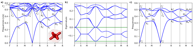
Figure 1: Band structures obtained from MPB and TETB model for a crystal with SG $Pn\bar{3}m$ (No. 224) without an external magnetic field applied. a) Dielectric structure of a crystal with SG $Pn\bar{3}m$ (No. 224) which its associated band structure [8]. b) Band structure obtained from the TB model. The bands enclosed by the pink rectangle belong to the additional modes included to regularize the symmetry content at $\Gamma$. c) Band structure obtained from the TB model after applying the mapping to the electromagnetic-wave equation frequency and imposing the transversality constraint.

For illustrative purposes, and as was mentioned in the introduction, we will develop a realistic example of the crystal depicted in the inset of Fig. 1a with SG No. 224 ($Pn\bar{3}m$). Such a crystal is a fully-connected geometry composed of dielectric rods arranged along the main diagonals of the cube. By analyzing the symmetry properties of the electromagnetic modes at the HSP, we compute the symmetry vector for the lowest six active bands of the photonic crystal, which returns:

$$\mathbf{v}^{T}=[ (\blacksquare)^{2T}+\Gamma_{2}^{-}+\Gamma_{4}^{-},R_{4}^{-}+R_{5}^{+},$$

$$M_{1}+2M_{4},X_{1}+X_{3}+X_{4}].$$ (9)

To illustrate better the full procedure, let us start by solving the Diophantine equation for $\mathbf{v}^{T}$ without any minimization. To this end, we solve the problem via the use the Moore-Penrose pseudo-inverse, by making $\textbf{z}=0$ in Eq. (5), obtaining the following vector with $N_{EBR}=25$ components:

$$\textbf{n}=(-1,0,0,0,0,1,0,0,2,0,0,-1,0,$$

$$\hskip 48.36958pt0,0,0,0,0,0,0,0,0,0,0,0)$$ (10)

which, in the notation of BCS, corresponds to the following combination of EBRs:

$$n_{A_{1}@2a}=-1,$$

$$n_{A_{1g}@4b}=1,$$

$$n_{A_{2u}@4b}=2,$$

$$n_{A_{1g}@4c}=-1.$$ (11)

More compactly, this correspond to a vector which contains the following EBRs:

$$\{-A_{1}@2a,A_{1g}@4b,2A_{2u}@4b,-A_{1g}@4c\}.$$ (12)

As can be seen, the vector solution $\mathbf{n}$ contains certain negative EBR coefficients. For the lowest bands of 3D PhC, this situation can never be avoided since it relies on the intrinsic obstruction due to the $\Gamma$ point problem [17], which enforces the presence of at least one minus sign in the decomposition. The impossibility of expressing the lowest bands in a 3D PhC with only strictly positive coefficients is reminiscent of the concept of ‘fragility’ in topological band theory [31, 32, 33]. As we will demonstrate in Sec. II.3, this apparent ‘fragility’ can be exploited for the construction of a photonic TB, by reinterpreting the EBR with negative coefficients in terms of ‘auxiliary’ longitudinal modes ($\mathbf{v}^{L}$) able to regularize the $\Gamma$ point problem. This will result in an expression like the following:

$$\textbf{v}^{T}+\textbf{v}^{L}=\textbf{v}^{T+L}$$ (13)

where $\textbf{v}^{T+L}$ is a linear combination of EBRs with integer positive coefficients.

In this first example, using the result of Eq. (11), we can write:

$$\textbf{v}^{T}+A_{1}@2a+A_{1g}@4c=A_{1g}@4b+2A_{2u}@4b$$ (14)

Note that the vector solution provided by Eq. (10) has length $\sqrt{7}$ and it might not be the minimal one.

Therefore, in order to verify whether a solution with shorter length can be found, we now turn to Eq. (8), and solve the minimization problem with the use of the $\textbf{v}^{\prime}$ and $\textbf{A}^{\prime}$ defined for Eq. (7). With the objective of being more didactic, we include a step-by-step derivation of the process in the SM, including explicit expressions for A, $\textbf{v}^{T}$, $\textbf{A}^{\prime}$ and $\textbf{v}^{\prime}$.

Solving Eq. (8) for a $\mathbf{n}$ we find:

$$\textbf{n}=(0,0,0,0,0,0,0,0,0,0,0,0,0,$$

$$\hskip 48.36958pt0,0,0,0,0,0,-1,0,0,1,0,0)$$ (15)

which is the vector solution with minimal length $|\textbf{n}|=\sqrt{2}$ satisfying all the imposed constraints, and it corresponds to the following combination of EBRs:

$$n_{B_{2}@6d}=-1,$$

$$n_{B_{1}@12f}=1,$$ (16)

which corresponds to a vector that contains the following EBRs:

$$\{-B_{2}@6d,B_{1}@12f\}.$$ (17)

In other terms:

$$\textbf{v}^{T}+B_{2}@6d=B_{1}@12f$$ (18)

which shows that, via the addition of the auxiliary $B_{2}@6d$ EBR to the $\textbf{v}^{T}$ vector, we can build a minimal TB model of the photonic bands via a single EBR, $B_{1}@12f$.

Even though the resulting TB is minimal, the $B_{1}@12f$ is a high-dimensional EBR and it corresponds to $12$ ‘pseudo-orbitals’. Therefore, we are motivated to see whether a second-minimal solution exists, involving lower-dimensional EBRs, that can be more favorable for the derivation of a TB model. For this purpose, we search a second-minimal solution to Eq. (8), obtaining:

$$\textbf{n}=(-1,0,0,0,0,0,0,0,1,0,0,0,0,$$

$$\hskip 48.36958pt0,1,0,0,0,0,0,0,0,0,0,0)$$ (19)

which is the vector solution with second-minimal length $|\textbf{n}|=\sqrt{3}$ and it corresponds to the following combination of EBRs:

$$n_{A_{1}@2a}=-1,$$

$$n_{A_{2u}@4b}=1,$$

$$n_{A_{2u}@4c}=1.$$ (20)

which corresponds to a vector that contains the following EBRs:

$$\{-A_{1}@2a,A_{2u}@4b,A_{2u}@4c\}.$$ (21)

This allows us to write:

$$\textbf{v}^{T}+A_{1}@2a=A_{2u}@4b+A_{2u}@4c$$ (22)

which shows that the addition of the $\mathbf{v}^{L}=A_{1}@2a$ as auxiliary longitudinal modes to the $\textbf{v}^{T}$ vector returns a linear combination of EBRs with integer positive coefficients ($\textbf{v}^{T+L}=A_{2u}@4b+A_{2u}@4c$) which is a regular set that contains all the symmetry content of the transverse band-structure, while avoiding the singularity at $\Gamma$. $\textbf{v}^{T+L}$ will give us the Wyckoff positions and pseudo orbital characters of an effective Wannier basis for the construction of a precise TB model. Later, we will prove that the auxiliary longitudinal bands $\mathbf{v}^{L}$ can be removed by spectral deformation, tuning the TB parameters a posteriori.

Note that, as compared to Eq. (17), now a TB model can be constructed with solely two EBRs, $A_{2u}@4b$ and $A_{2u}@4c$, each of them having dimension $4$ and therefore using only $8$ pseudo-orbitals in total. Note as well that Eq. (22) allows us to assign a well-defined value to $(\blacksquare)^{2T}$ without any extra knowledge of the symmetry constraints at $\Gamma$. More specifically, we can obtain, a posteriori, that $(\blacksquare)^{2T}=\Gamma_{4}^{-}-\Gamma_{1}^{+}$, in agreement with Ref. [17]. In Sec. II.3, we will show how to construct a photonic TB starting from the result obtained in Eq. (22), interpreting the $A_{1}@2a$ EBRs as auxiliary ‘longitudinal’ modes.

Another example concerning SG $Pm\bar{3}m$ (No. 221) will be developed in the SM for illustrative purposes.

II.2 Solution by Real-space invariants

As an alternative approach to solve Eq. (3), we can adapt the theory of real space invarinats (RSIs) introduced in Refs. [34, 35]. RSIs are invariants computed from the multiplicities $\mathbf{m}$ of the occupied site symmetry group representations, or Wannier orbitals, at each Wyckoff position (WP). In particular, the RSIs parameterize whether or not two different configurations of occupied orbitals can be adiabatically deformed into each other without breaking the symmetries of the system. For both topologically trivial gapped bands and symmetry-indicated fragile topological bands, all RSIs take integer values. Finally, for gapless or topologically nontrivial bands, the RSIs take rational values [36, 34, 37]. In general, the number of unique RSIs in a space group will be smaller than the the number of EBRs. Additionally, as we will discuss below, a subset of the RSIs of every space group can be computed from the symmetry vector in momentum space.

Exploiting this, we will see below that we can combine the position and momentum space expressions for the RSIs to solve Eq. (3). The solution procedure is as follows: We will first complete the symmetry vector in momentum space at the $\Gamma$ point $(\blacksquare)^{2T}$, based on the result in Ref. [17]. Next, we compute all RSIs that can be determined from the symmetry vector, including enough photonic bands to ensure we get integers for all RSIs. Since there are fewer RSIs than there are EBRs, this gives us a smaller set of Diophantine equations which we can solve analytically for the occupied site symmetry group representations at each WP.

To see how this works, we will first analyze the RSIs of photonic crystals in SG $P2$ (No. 3) in Sec. II.2.1, as a simple example of the procedure. Then, in Sec. II.2.2 we will apply this machinery to solve Eq. (3) for our photonic crystal in Fig. 1a.

II.2.1 Photonic RSIs in Space Group $P2$

Let us consider SG $P2$ (No. 3) as the most simple space group one can take for a clear discussion on RSI. We will follow the notation used in the BCS [25] during the extension of the work. The SG $P2$ is generated by a twofold rotation, $C_{2y}:(x,y,z)\to(x,-y,z)$, and three translations by the primitive lattice vectors, $\mathbf{t}_{1}=\hat{x}$, $\mathbf{t}_{2}=\hat{y}$, and $\mathbf{t}_{3}=\hat{z}$. SG $P2$ has four maximal WPs denoted by $\mathbf{q}=1a$, $1b$, $1c$, and $1d$. There site-symmetry groups $G_{\mathbf{q}}$ are $G_{1a}=\{C_{2y}|\mathbf{0}\}$, $G_{1b}=\{C_{2y}|\mathbf{t}_{3}\}$, $G_{1c}=\{C_{2y}|\mathbf{t}_{1}\}$, and $G_{1d}=\{C_{2y}|\mathbf{t}_{1}+\mathbf{t}_{3}\}$, respectively. Also, a generic WP $2e$ which has a trivial site-symmetry group $G_{2e}=\{E|\mathbf{0}\}$. Note that the representative positions of WPs are $1a:(0,y,0)$, $1b:(0,y,1/2)$, $1c:(1/2,y,0)$, $1d:(1/2,y,1/2)$, and $2e:\{(x,y,z),(-x,y,-z)\}$, where $x,y,z$ are free parameters. This indicates that changing the position of the orbital through those parameters preserves the symmetries imposed by the SG and the topology of the system. The coordinates and site symmetry groups for these Wyckoff positions are summarized in Table 1.

WP ($\mathbf{q}$)	Coordinates	$G_{\mathbf{q}}$
$1a$	$(0,y,0)$	$\{C_{2y}|\mathbf{0}\}$
$1b$	$(0,y,1/2)$	$\{C_{2y}|\mathbf{t}_{3}\}$
$1c$	$(1/2,y,0)$	$\{C_{2y}|\mathbf{t}_{1}\}$
$1d$	$(1/2,y,1/2)$	$\{C_{2y}|\mathbf{t}_{1}+\mathbf{t}_{3}\}$
$2e$	$(x,y,z)$,	$\{E|\mathbf{0}\}$
	$(-x,y,-z)$

Irrep ($\rho$)	$1$	$C_{2}$
$A$	$1$	$1$
$B$	$1$	$-1$

Table 1: Left: Wyckoff positions (WPs) of SG $P2$. $G_{\mathbf{q}}$ denotes site-symmetry group of WP $\mathbf{q}$. Right: Irreducible representations $\rho$ of point group $C_{2}$.

In this SG, any orbital $\rho_{\mathbf{q}}$ localized at a maximal WP q ($\mathbf{q}=1a$,$1b$,$1c$,$1d$) transforms as either $\rho=A$ or $B$ representation of the point group $C_{2}$, which is isomorphic to $G_{\textbf{q}}$. (See Table 1.) $A$ has eigenvalue $+1$ while $B$ has $-1$ with respect to $C_{2}$ We denote the multiplicity of each orbital as $m(\rho_{\mathbf{q}})$. Any band representation (BR) corresponding to a topologically trivial band can be induced from a set of orbitals located at maximal WPs. Consequently, for a given trivial BR, one can assign a set of multiplicities that correspond to such orbitals. We will denote this set as $\{m(\rho_{\mathbf{q}})\}$.

However, as we will see, $\{m(\rho_{\mathbf{q}})\}$ may not be uniquely determined since each $m(\rho_{\mathbf{q}})$ is not invariant under adiabatic deformations that preserve band topology. Nevertheless, some linear combinations of $m(\rho_{\mathbf{q}})$-s may remain invariant under such transformations. In the study of crystalline materials, these invariant linear combinations are known as RSIs.

We will now show how to derive the RSIs in SG $P2$. We know that a single orbital at one of the maximal Wyckoff positions transforming in either the $A$ or $B$ representation of $G_{\mathbf{q}}$ cannot be moved adiabatically to a different Wyckoff position; only the $y$ coordinate of the maximal Wyckoff positions is a free parameter. On the contrary, if we have two orbitals, one $A_{1a}$ and one $B_{1a}$, they can be hybridized into a pair of $C_{2y}$-related orbitals. For clear illustration, let us denote the two orbitals transforming as $A_{1a}$ and $B_{1a}$ as $\phi_{A_{1a}}$ and $\phi_{B_{1a}}$ respectively. Then, their linear combinations $\Phi_{\pm}=\frac{1}{\sqrt{2}}(\phi_{A_{1a}}\pm\phi_{B_{1a}})$ are related by $C_{2y}$ to each other. In this case, $\Phi_{+}$ and $\Phi_{-}$ can move to $(x,y,z)$ and $(-x,y,-z)$ respectively because their configuration respects $C_{2y}$ for any value of free parameters $(x,y,z)$, which characterize the generic WP $2e$. Hence, these hybridized orbitals $\Phi_{\pm}$ can be adiabatically moved to the WP $2e$ and become $A_{2e}$ while respecting the symmetry properties, and topology of the band representation. Conversely, an $A_{2e}$ orbital can be deformed into a pair of $A_{1a}+B_{1a}$ orbitals. Hence, in the adiabatic processes, neither $m(A_{1a})$ nor $m(B_{1a})$ are invariant. However, the difference $-m(A_{1a})+m(B_{1a})$ remains invariant. Since there is no adiabatic process that can change $-m(A_{1a})+m(B_{1a})$, it must be a topological invariant in SG $P2$. We thus identify it with a real space invariant which we call $\delta_{1a}$.

Repeating the preceding analysis for the other maximal Wyckoff positions allows us to define the RSIs for space group $P2$ as

$$\delta_{1a}=-m(A_{1a})+m(B_{1a}),$$

$$\delta_{1b}=-m(A_{1b})+m(B_{1b}),$$

$$\delta_{1c}=-m(A_{1c})+m(B_{1c}),$$

$$\delta_{1d}=-m(A_{1d})+m(B_{1d}).$$ (23)

For this definition, we can easily deduce which WPs must be occupied by Wannier orbitals, based on nonzero RSIs. By construction, when it is possible to move every orbital at a WP $\mathbf{q}$ to other WP(s), $\delta_{\mathbf{q}}$ is zero. Thus, if an RSI $\delta_{\mathbf{q}}$ is nonzero, the relevant WP $\mathbf{q}$ must be occupied by least by one orbital. In other words, a nonzero RSI indicates the existence of symmetry-pinned orbital(s) at the corresponding WP. The above discussion about adiabatic deformations can be translated into subgroup-group and induction-subduction relations. For a general discussion on RSI, we refer the reader to Ref. [37]. The RSIs for every magnetic and nonmagnetic SGs have been tabulated in the past and are enumerated in Ref. [37] and the BCS [25].

The RSIs in Eq. (23) are defined in terms of orbitals localized in real space. This formulation of RSIs are called the local RSIs [37]. In the case of SG $P2$, all four local RSIs can be completely determined by the multiplicities of the momentum-space irreps, i.e. in terms of the symmetry vector $\mathbf{v}$ [38, 36, 34, 37, 25]. To construct a mapping between the RSIs and multiplicities of Wannier orbitals, we define $\boldsymbol{\delta}=(\delta_{1a},\delta_{1b},\delta_{1c},\delta_{1d})^{T}$ and

$$\mathbf{m}= [m(A_{1a}),m(B_{1a}),m(A_{1b}),m(B_{1b}),$$

$$m(A_{1c}),m(B_{1c}),m(A_{1d}),m(B_{1d})]^{T}.$$ (24)

Then, Eq. (23) can be rewritten as

$$\boldsymbol{\delta}=\begin{pmatrix}-1&1&0&0&0&0&0&0\\ 0&0&-1&1&0&0&0&0\\ 0&0&0&0&-1&1&0&0\\ 0&0&0&0&0&0&-1&1\end{pmatrix}\mathbf{m}.$$ (25)

A set of Wannier orbitals with multiplicities $\mathbf{m}$ induces a BR with symmetry vector $\mathbf{v}$. In Eq. (24), $\mathbf{m}$ counts the multiplicities of all types of Wannier orbitals at maximal WPs. Note that $\mathbf{m}$ coincides with $\mathbf{n}$ defined in Eq. (7) except in exceptional cases defined in Ref. 14. (In such cases, $\mathbf{n}$ contains only site-symmetry group representations at a subset of maximal WPs that is sufficient to generate all EBRs. In most cases, this coincides with the set of all maximal WPs). Because a EBR is induced by a Wannier orbital at a maximal WP, $\mathbf{v}$ can be computed by the EBR matrix $\mathbf{A}$ in $P2$ such that $\mathbf{v}=\mathbf{A}\textbf{m}$. Thus, for a given symmetry vector $\mathbf{v}$, $\mathbf{m}$ can be solved by Eq. (5). Explicitly, Eq. (5) yields

$$m(A_{1a}) =\frac{1}{2}(-n_{\Gamma_{1}}+n_{A_{1}}+n_{B_{1}}+n_{C_{1}})-z_{4}-z_{6}-z_{8},$$

$$m(A_{1b}) =\frac{1}{2}(n_{\Gamma_{1}}-n_{A_{1}}-n_{B_{1}}+n_{C_{1}})+z_{4},$$

$$m(A_{1c}) =\frac{1}{2}(n_{\Gamma_{1}}-n_{A_{1}}+n_{B_{1}}-n_{C_{1}})+z_{6},$$

$$m(A_{1d}) =\frac{1}{2}(n_{\Gamma_{1}}+n_{A_{1}}-n_{B_{1}}-n_{C_{1}})+z_{8},$$

$$m(B_{1a}) =n_{\Gamma_{2}}-z_{4}-z_{6}-z_{8},$$

$$m(B_{1b}) =z_{4},\quad m(B_{1c})=z_{6},\quad m(B_{1d})=z_{8}.$$ (26)

Here, $\Gamma$, $A$, $B$ and $C$ refer to the HSPs of SG $P2$, and $\Gamma_{1,2}$, $A_{1,2}$, $B_{1,2}$, and $C_{1,2}$ refer to little group irreps in the BCS notation. Also, $n_{\rho_{\mathbf{k}}}$ denotes the multiplicity of the irrep $\rho_{\mathbf{k}}$, and $z_{4,6,8}$ are free integer parameters defined in Eq. (5).

Substituting Eq. (26) into Eq. (25), we obtain

$$\delta_{1a}=n_{\Gamma_{2}}+\frac{1}{2}\left(n_{\Gamma_{1}}-n_{A_{1}}-n_{B_{1}}-n_{C_{1}}\right),$$

$$\delta_{1b}=\frac{1}{2}\left(-n_{\Gamma_{1}}+n_{A_{1}}+n_{B_{1}}-n_{C_{1}}\right),$$

$$\delta_{1c}=\frac{1}{2}\left(-n_{\Gamma_{1}}+n_{A_{1}}-n_{B_{1}}+n_{C_{1}}\right),$$

$$\delta_{1d}=\frac{1}{2}\left(-n_{\Gamma_{1}}-n_{A_{1}}+n_{B_{1}}+n_{C_{1}}\right).$$ (27)

Let us emphasize that Eq. (27) is uniquely determined from the symmetry data, while each multiplicity of Wannier orbital in Eq. (26) depends on free parameters $z_{4,6,8}$.

For a general space group, there may be additional RSIs defined only modulo integers which cannot be determined uniquely from the momentum space symmetry vector. In these cases, linear combinations of RSIs can be constructed that are determined uniquely from the symmetry vector; these linear combinations are known as composite RSIs and are tabulated in Ref. [37]. When local RSIs cannot be determined from symmetry vector, their linear combinations can be computed instead. Such modified RSIs are called composite RSIs [37], and they count the multiplicities of orbitals at multiple WPs.

In the previous discussion, we introduced RSIs in general terms for a simple SG. Our objective now, is to compute them to derive a set of pseudo-orbital that yields a given symmetry vector $\mathbf{v}^{T}$ . To compute the RSIs from a given symmetry vector $\mathbf{v}^{T}$ of a 3D photonic band structure, some additional information on $(\blacksquare)^{2T}$ is necessary. Maxwell’s equations and symmetry-compatibility relations along high-symmetry lines and planes impose strong conditions on $(\blacksquare)^{2T}$ [28, 17]. That is, transverse ($2T$) modes need to be expressible as the difference between the vector and the trivial representations of the little group of $\Gamma$. As a result, $(\blacksquare)^{2T}$ can be expressed as a linear combination of irreps $\rho_{i[\Gamma]}$, i.e. $(\blacksquare)^{2T}=\oplus_{i}n_{i[\Gamma]}\rho_{i[\Gamma]}$, where $n_{i[\Gamma]}$ can be a negative integer. The particular expressions of $(\blacksquare)^{2T}$ depend on the given SG, and this information is listed in Ref. [17] for the 230 SGs. RSIs were originally implemented for “regular” irrep multiplicities ($n_{i[\Gamma]}\geq 0$). Nevertheless, although $(\blacksquare)^{2T}$ can be irregular, meaning that some irreps can have negative multiplicities ($n_{i[\Gamma]}<0$), RSIs can still be computed. This is so because the RSIs are defined by a (linear) equation between some matrix and $n_{i[\mathbf{k}]}$.

Now, let us explain how the RSI analysis can solve the Diophantine equation in Eq. (7) efficiently. For this, we consider two possible examples of $\mathbf{v}^{T}$ in SG $P2$; $\mathbf{v}^{(1)}=[(\blacksquare)^{2T},2A_{1},B_{1}+B_{2},2C_{1},D_{1}+D_{2},2E_{1},2Y_{1},2Z_{2}]$ and $\mathbf{v}^{(2)}=[(\blacksquare)^{2T},2A_{1},2B_{1},2C_{1},2D_{1},2E_{1},2Y_{1},2Z_{2}]$. Both have the dimension ${\rm dim}(\mathbf{v}^{T})=2$. First, note that $(\blacksquare)^{(2T)}=2\Gamma_{2}$ in SG $P2$ [28, 17]. Then, by using Eq. (27), the RSI indices $\boldsymbol{\delta}=(\delta_{1a},\delta_{1b},\delta_{1c},\delta_{1d})$ can be computed for $\mathbf{v}^{(1,2)}$ simply following Eq. (23). In the case of $\mathbf{v}^{(1)}$, the corresponding RSI indices are $\boldsymbol{\delta}^{(1)}=(-1/2,1/2,3/2,1/2)$. When at least one RSI in $\boldsymbol{\delta}$ is fractional, i.e. $\boldsymbol{\delta}^{(1)}\notin\mathbb{Z}^{4}$, $\mathbf{v}^{(1)}$ has stable topology with nontrivial symmetry indicator and does not allow integer-valued $\mathbf{n}$ or $m(\rho_{\mathbf{q}})$. Thus, $\mathbf{v}^{(1)}$ is not Wannierizable. Instead, one can consider a bigger set including higher energy bands with symmetry vector $\mathbf{v}^{\prime}$ such that $\mathbf{v}^{(1)}+\mathbf{v}^{\prime}$ corresponds to integer-valued RSI indices $\boldsymbol{\delta}$ and allows the Wannierzation.

On the other hand, $\mathbf{v}^{(2)}$ has an integer-valued RSIs with $\mathbf{\delta}^{(2)}=(-1,1,1,1)$. This implies

$$-m(A_{1a})+m(B_{1a})=-1,$$

$$-m(A_{1b})+m(B_{1b})=1,$$

$$-m(A_{1c})+m(B_{1c})=1$$

$$-m(A_{1d})+m(B_{1d})=1.$$ (28)

To solve these equations, we assume that all the orbitals are localized at maximal WPs $\mathbf{q}=1a,1b,1c,1d$ because orbitals at any non-maximal WP can always be moved to $\mathbf{q}$. With this assumption, ${\rm dim}(\mathbf{v}^{(2)})=2$ imposes $\sum_{\mathbf{q}}\sum_{\rho=A,B}m(\rho_{\mathbf{q}})=2$. One can easily find a particular solution, $m(A_{1a})=m(B_{1b})=m(B_{1c})=1$, $m(A_{1d})=-1$, and thus we express $\mathbf{v}^{(2)}$ as

$$\mathbf{v}^{(2)}=A@1a+B@1b+B@1c-A@1d.$$ (29)

This implies that one can construct a TB model for the photonic bands corresponding to $\mathbf{v}^{(2)}$ by introducing an auxiliary pseudo-orbital $A_{1d}$. Note that, to regularize the polarization singularity at $\Gamma$ by adding auxiliary band(s), the auxiliary band must span the trivial irrep [17]. Consistent with this condition, $A_{1d}$ orbital induces the EBR $A@1d$ with the trivial irrep $\Gamma_{1}$.

II.2.2 Photonic RSIs in Space Group $Pn\bar{3}m$

Let us consider, again, the crystal shown in Fig. 1 with SG $Pn\bar{3}m$ (No. 224). In this SG, there are 5 maximal WPs: $2a:(1/4,1/4,1/4)$ with site-symmetry group $G_{2a}=\bar{4}3m$, $4b:(0,0,0)$ with $G_{4b}=\bar{3}m$, $4c:(1/2,1/2,1/2)$ with $G_{4c}=\bar{3}m$, $6d:(1/4,3/4,3/4)$ with $G_{6d}=\bar{4}2m$, and $12f:(1/2,1/4,3/4)$ with $G_{12f}=222$. For these maximal WPs, the RSIs are [37]

$$\delta_{a}=m(A_{1})-m(A_{2})-m(T_{2})+m(T_{1}),$$

$$\delta_{d}=-m(A_{1})+m(B_{1})+m(B_{2})-m(A_{2}),$$

$$\delta_{f}=m(A_{1})+m(B_{1})-m(B_{3})-m(B_{2})\quad({\rm mod}\,2),$$

$$\delta_{\mathbf{q},1}=m(A_{1g})-m(A_{1u})+m(A_{2g})-m(A_{2u}),$$

$$\delta_{\mathbf{q},2}=-m(E_{g})+m(E_{u}),$$ (30)

where $\mathbf{q}=b,c$. (We omit the multiplicities of WPs for simpler notation.) RSIs can also be defined for nonmaximal WPs ($8e,12g,24h,24i,24j,24k$). To avoid complications, let us focus on the RSIs defined in Eq. (30) for the maximal WPs $a,b,c,d,f$, because any orbitals at nonmaximal WPs can be adiabatically moved to the maximal WPs . We denote those RSIs as $\tilde{\boldsymbol{\delta}}=(\delta_{a},\delta_{b,1},\delta_{b,2},\delta_{c,1},\delta_{c,2},\delta_{d},\delta_{f})$ collectively. This reduced set of RSIs $\tilde{\boldsymbol{\delta}}$ can be uniquely computed from a given symmetry vector $\mathbf{v}^{T}$, and the mapping from $\mathbf{v}^{T}$ to $\tilde{\boldsymbol{\delta}}$ is accessible via the BCS [25].

As we did in Sec. II.1, from the analysis of the symmetry properties of the Bloch electromagnetic modes supported by the PhC (see Fig. 1a), we obtain the following symmetry vector:

$$\mathbf{v}^{T}=[ (\blacksquare)^{2T}+\Gamma_{2}^{-}+\Gamma_{4}^{-},R_{4}^{-}+R_{5}^{+},$$

$$M_{1}+2M_{4},X_{1}+X_{3}+X_{4}].$$ (31)

which is representative of the lowest 6 active bands in the photonic spectrum. Being consistent with the symmetry-constrained irrep content $\Gamma$ proposed by Ref. [17], $(\blacksquare)^{2T}=\Gamma_{4}^{-}-\Gamma_{1}^{+}$. For $\mathbf{v}^{T}$ the RSI indices are $\tilde{\boldsymbol{\delta}}=(-1,-1,0,-1,0,0,0)$. Thus, only the three RSIs related to WP $a,b,c$ are nonzero, i.e. $\delta_{a}=\delta_{b,1}=\delta_{c,1}=-1$. To solve the RSI equations (Eq. (30)), we further use ${\rm dim}(\mathbf{v}^{T})=6$ and the irreps at $\Gamma$, which are $-\Gamma_{1}^{+}+\Gamma_{2}^{-}+2\Gamma_{4}^{-}$. As a result, we find that $\mathbf{v}^{T}$ can be expressed as

$$\mathbf{v}^{T}=A_{2u}@{4b}+A_{2u}@{4c}-A_{1}@{2a}.$$ (32)

Thus, proceeding as detailed in the following section, we will be able to construct a TETB model for this system by placing $A_{2u}$ orbitals at WPs $4b$ and $4c$ and introducing auxiliary longitudinal modes corresponding to $A_{1}@2a$.

Another example concerning SG $Pm\bar{3}m$ (No. 221) is developed in the SM.

II.3 Mapping to a photonic TETB

Once a set of candidate pseudo-orbitals have been determined following either method A or B, we move to the construction of a TB model based on them. We look for a TB model which satisfies the following conditions: the additional degrees of freedom introduced as longitudinal modes ($\mathbf{v}^{L}$) represent energy bands away from the active bands; the TB model captures the features of the transverse bands ($\mathbf{v}^{T}$) in the energy window of interest; the model reproduces the $(\blacksquare)^{2T}$ obstruction at $\Gamma$ as well as all the symmetry, topology and energetic features of the active bands in the PhC.

To proceed, we exploit a formal mapping between the cell-periodic Schrödinger and the Maxwell wave equation, which are respectively linear and quadratic in time. This allows us to relate the energy $\mathcal{E}$ of the electronic wavefunction $\phi(\mathbf{r})$ in presence of a crystal periodic potential $V(\mathbf{r})$:

$$[\frac{-\hbar^{2}}{2m}\left(\gradient\right)^{2}+V(\mathbf{r})]\phi(\mathbf{r})=\mathcal{E}\phi(\mathbf{r})$$ (33)

and the frequency of light $\omega$ in media with periodic dielectric permittivity $\varepsilon(\mathbf{r})$:

$$\gradient\times\left(\frac{1}{\varepsilon(\mathbf{r})}\gradient\times\mathbf{H}(\mathbf{r})\right)=\left(\frac{\omega}{c}\right)^{2}\mathbf{H}(\mathbf{r})$$ (34)

according to $\mathcal{E}\sim\omega^{2}$ [40].

This quadratic mapping allows us to construct an effective solid-state inspired optical 3D TB model by enforcing the eigenvalues ($\Omega$) of the set of transversal bands to fulfil $\Omega=\omega^{2}\geq 0$ and the lowest set of longitudinal bands to fulfil $\Omega=\omega^{2}\leq 0$. Note that since the frequency of the electromagnetic solutions is $\omega=\sqrt{\Omega}$, the final real spectra will not contain the auxiliary nonphysical modes. Forcing the longitudinal modes and active transverse modes to be isolated from each other except at $\Omega=0$, enables us to achieve all the previous points.

To construct a reliable TB which satisfies all the aforementioned constraints, we proceed via a four-step strategy:

1. From the EBR decomposition obtained from the method in either Sec. II.1 or Sec. II.2, we identify $\textbf{v}^{L}$ and $\textbf{v}^{T+L}$.

2. We build a TB model with generic free parameters from EBRs with the orbital character and Wyckoff positions as dictated by $\textbf{v}^{T+L}$.

3. We analyze the symmetry content of the bands induced by these orbitals and identify which modes can be associated uniquely to $\textbf{v}^{L}$.

4. We tune the parameters of the TB (onsite energies and hoppings) to simultaneously satisfy two constraints: we enforce the set of longitudinal bands to be the lowest energy modes and force their eigenvalues ($\Omega$) to fulfil $\Omega=\omega^{2}\leq 0$. We then fit the $\Omega=\omega^{2}>0$ bands to the square of the electromagnetic frequencies obtained by numerical solutions of PhC.

This will result in a Transversality-Enforced Tight-Binding (TETB) model, with Hamiltonian $H(\textbf{k})$, which captures all the symmetry, topology and energetic features of the transverse bands in the PhC.

To illustrate this strategy, we follow again the guiding example of Fig. 1a with SG No. 224 and the symmetry vector showed in Eq. (II.1).

Since we have already obtained the EBR decomposition of this symmetry vector in Eq. (22), we can perform a TB model by placing pseudo-orbitals that transform as $A_{2u}$ in WPs $4c:(1/2,1/2,1/2)$ and $4b:(0,0,0)$. This model gives rise to a TB Hamiltonian which can be expressed as a $8\times 8$ matrix with nine free-parameters up to third-nearest neighbors: $\alpha_{1}$ and $\alpha_{2}$, which correspond to the on-site energies; $a_{1}$, is the nearest neighbour hopping; $a_{2}$, $r_{2}$, $s_{2}$ and $w_{2}$, are the second-nearest neighbor hoppings; and, $a_{3}$ and $r_{3}$, are the third-nearest neighbor hoppings. The specific expression of the Hamiltonian can be seen in the SM. Those free-parameters are adjusted in order to fit the band structure of the crystal, shown in Fig. 1a, and forcing the additional nonphysical bands to have negative eigenvalues, obtaining the coefficients shown in Table 2.

Parameters	Value
$\alpha_{1}$	0.306159
$\alpha_{2}$	0.123753
$a_{1}$	0.157927
$a_{2}$	-0.064197
$r_{2}$	0.068848
$s_{2}$	-0.100771
$w_{2}$	0.022712
$a_{3}$	0.035449
$r_{3}$	-0.041474

Table 2: Parameters of the TB Hamiltonian for SG $Pn\bar{3}m$ (No. 224).

We perform the fitting by applying a least square minimization routine at all HSPs. The cost function is a multiobjective, multivariable function, which measures the distances between the square of the frequencies computed numerically in MPB for the PhC and the eigenvalues of the TETB, for each irrep. The objective vector contains the multiple distances between the eigenvalues, with the same irrep at each HSP. The variables are the TETB coefficients. Specifically, we use the least-squares function of the scipy.optimize package in Python [41] and we selected only some irreps at HSPs as minimization objectives.

The resulting TETB Hamiltonian $H(\textbf{k})$ is shown in the SM.

In Fig. 1b, the eigenvalues of the TB model are shown. The longitudinal bands are marked between the green lines. They show negative eigenvalues and are detached from the physical, transversal ones. Finally, taking the square root of the eigenvalues, as $\Omega=\omega^{2}$, we discard the longitudinal modes in the real TETB band-structure and achieve the physical band structure shown in Fig. 1c which is composed by exclusively transverse modes. As it can be seen, the TETB band-structure reproduces the MPB band structure of the crystal faithfully for the six lowest energy bands, both in their dispersion and symmetry content.

Another, more detailed example concerning SG $Pm\bar{3}m$ (No. 221) will be developed in the SM where we include a detailed step-by-step derivation of the procedure.

II.4 Introducing a magnetic field into the model

Some of the most important applications of topological photonics rely on Time Reversal Symmetry (TRS) breaking, since it stabilizes strong topology in Cartan–Altland–Zirnbauer (CAZ) ten-fold classification of topological materials [42, 43] Usually, TRS breaking in photonic crystals is achieved by the use of gyroelectric or gyromagnetic materials, either in the presence of an external static magnetic field or equivalently through intrinsic remnant magnetization. To mimic such effects, here, we develop a general method to simulate in our TETB models the interaction of an external and static magnetic field with a PhC.

Usually, in solid-state TB models, the effects of a static magnetic field are introduced via minimal or non-minimal coupling methods. The minimal coupling method, which proceeds through the Peierls substitution [44, 45], is usually adopted in electronic systems but it is here forbidden due to the uncharged nature of photons. This forces us to use non-minimal coupling techniques. Non-minimal coupling methods include the magnetic field as a perturbation in the response of the system. Accordingly, the Hamiltonian with the effect of the magnetic field can be represented by:

$$H_{B}(\textbf{k},\textbf{B})=H(\textbf{k})+f(\textbf{k},\textbf{B}),$$ (35)

where $\mathbf{k}$ and B are the momentum and magnetic field vectors, respectively; $H(\textbf{k})$ is the TETB Hamiltonian in momentum space in presence of TRS; and $f(\mathbf{k},\textbf{B})$ is a function depending on the components of B. The function $f(\textbf{k},\textbf{B})$ should respect the symmetries of the crystal which will constrain its form. In most cases, taking $f(\textbf{k},\textbf{B})$ as a linear function on the components of B is enough to model the effect of the magnetic field. Nevertheless, higher orders in $f(\textbf{k},\textbf{B})$ can be considered to reproduce the effects of higher magnetic field intensities if necessary.

Coming back to the example of the crystal with SG $Pn\bar{3}m$ (No. 224), for which we constructed a TETB model in the previous section, now we will apply an external static magnetic field along $z$ to it. As shown in [8], the introduction of a $z$-directed gyroelectric bias in this system gives rise to a topological charge-1 Weyl dipole oriented along the $k_{z}$ axis. To model this phenomenon via the TETB, we will apply a first-order in the perturbation in B. Such perturbation $f_{L}(\textbf{k},\textbf{B})$ must transform as follows for any symmetry transformation $g$ of SG $Pn\bar{3}m$ (No. 224):

$$gf_{L}(\textbf{k},\textbf{B})g^{-1}=f_{L}(g\textbf{k},g\textbf{B}).$$ (36)

This constraint introduces five free-parameters into the TB hamiltonian $H_{B}(\textbf{k},\textbf{B})$: $\delta_{1}$, which enters in the first-nearest neighbor hopping terms. Similarly, parameters $\delta_{2}$, $\beta_{2}$, $\kappa_{2}$ and $\epsilon_{2}$, enter in the expressions of the second-nearest neighbor hoppings. Due to symmetry constraints, the third nearest neighbour hoppings are not affected by this perturbation at first order.

Now, those free parameters need to be adjusted in order to fit the MPB band structure of the crystal affected by the static magnetic field (shown Fig. 2a). Proceeding similarly as in the previous section, we apply the same minimization routine over the new parameters, leaving the previous TETB parameters (Table. 2) unaltered. We obtain the values shown in Table 3 for the perturbation. The corresponding magnetic TETB Hamiltonian $H(\textbf{k},\textbf{B})$ is shown in the SM.

Fig. 2b displays the eigenvalues of the perturbed TETB model with a magnetic field along $z$. Again we marked the longitudinal auxiliary bands between green lines, observing that, in fact, they retain negative eigenvalues.

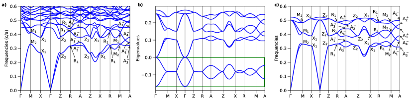
Figure 2: Band structures obtained from MPB and TETB model for a crystal with SG $Pn\bar{3}m$ (No. 224) with an external magnetic field applied along $z$. a) Frequency bands obtained from the crystal with a magnetic field applied along $z$. b) Band structure obtained from the TB model with a magnetic field applied along $z$. The bands enclosed by the pink rectangle belong to the additional modes included to regularize the symmetry content at $\Gamma$. c) Frequency bands obtained from the TB model with a magnetic field applied along $z$.

Parameters	Value
$\delta_{1}$	0
$\delta_{2}$	$0.001i$
$\beta_{2}$	$-0.001i$
$\kappa_{2}$	$0.001i$
$\epsilon_{2}$	$-0.001i$

Table 3: Parameters of the linear function $f_{L}(\textbf{k},\textbf{B})$.

Finally, using $\Omega=\omega^{2}$, we discard the longitudinal modes obtaining the desired band structure, shown in Fig. 2c. The obtained bandstructure reproduces perfectly the one obtained through exact numerical simulations. Note that in the MPB simulations the applied magnetic field gives rise to the generation of a pair of Weyl points [8], one of which is localized exactly at half of the MA high symmetry line. This behaviour is perfectly replicated by the TETB model, as shown in Fig 3.

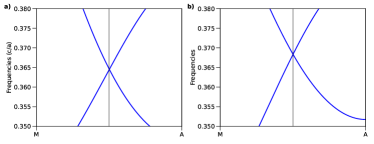
Figure 3: Position of the Weyl point obtained from MPB and TB model for a crystal with SG $Pn\bar{3}m$ (No. 224) in perfect agreement with Ref. [8]. a) Weyl point situated at exactly half the MA line for the MPB computations. b) Weyl point situated at exactly half the MA line for the TB model.

III Conclusions

In summary, in this article, we propose the first method to construct a reliable TB representation of 3D PhCs, even if maximally localized WFs do not exist for such systems [15]. We show how this can be achieved by developing a transversality-enforced tight-binding model (TETB) capable of capturing and regularizing the $\Gamma$-point electromagnetic obstruction that arises due to the transversality constraint of Maxwell equations, while accurately reproducing the symmetries of the PhC. This method proceeds via the addition of auxiliary longitudinal modes to the physical transverse bands of the 3D PhC [17]. To identify optimal pseudo-orbital candidates for the TETB, we propose two different strategies, a numerical and an analytical approach. The numerical approach proceeds via a linear optimization routine while the analytical method is based on calculations of RSIs. By establishing a formal mapping between the Maxwell and Schrödinger equations, we are able to finally discard the nonphysical longitudinal modes. The resulting TETB is shown to be able to reproduce all the symmetry, topology and energetic dispersion of the transverse bands in the PhC accurately. Finally, we show how to model gyrotropy by providing a magnetic version of our TETB model using non-minimal coupling.

In conclusion, our work provides the first systematic method to analytically model the photonic bands of the lowest transverse modes over the entire BZ via a TETB model. The lower-computational cost of TB models in comparison with exact Maxwell solvers will allow increasing the complexity of future theoretical developments in the field of topological photonics via the calculation of extensive supercells. For example, recently, this method allowed us to simulate the higher-order response on the hinges of photonic axion insulators [46]. This development was only possible by the use of TETB models because the calculation of $xy$-confined rod-geometries of 3D supercells was out of reach for state-of-the-art high-performance computing clusters.

Therefore we believe that our TETB will facilitate the study of boundary responses of future photonic topological phases, particularly in the case of 3D PhC.

Acknowledgements

A.G.E. and C.D. acknowledges support from the Spanish Ministerio de Ciencia e Innovación (PID2019-109905GA-C2). M.G.D., A.M.P. and M.G.V. acknowledge the Spanish Ministerio de Ciencia e Innovacion (grant PID2019-109905GB-C21). A.G.E. and M.G.V. acknowledge funding from the IKUR Strategy under the collaboration agreement between Ikerbasque Foundation and DIPC on behalf of the Department of Education of the Basque Government, Programa de ayudas de apoyo a los agentes de la Red Vasca de Ciencia, Tecnología e Innovación acreditados en la categoría de Centros de Investigación Básica y de Excelencia (Programa BERC) from the Departamento de Universidades e Investigación del Gobierno Vasco and Centros Severo Ochoa AEI/CEX2018-000867-S from the Spanish Ministerio de Ciencia e Innovación. M.G.V. thanks support to the Deutsche Forschungsgemeinschaft (DFG, German Research Foundation) GA 3314/1-1 – FOR 5249 (QUAST) and partial support from European Research Council (ERC) grant agreement no. 101020833. The work of JLM has been supported in part by the Basque Government Grant No. IT1628-22 and the PID2021-123703NB-C21 grant funded by MCIN/AEI/10.13039/501100011033/ and by ERDF; “A way of making Europe”. The work of B.B. and Y. H. is supported by the Air Force Office of Scientific Research under award number FA9550-21-1-0131. Y. H. received additional support from the US Office of Naval Research (ONR) Multidisciplinary University Research Initiative (MURI) grant N00014-20-1-2325 on Robust Photonic Materials with High-Order Topological Protection. C.D. acknowledges financial support from the MICIU through the FPI PhD Fellowship CEX2018-000867-S-19-1. M.G.D. acknowledges financial support from Government of the Basque Country through the pre-doctoral fellowship PRE_2022_2_0044.

References

- [1] Sajeev John. Strong localization of photons in certain disordered dielectric superlattices. Phys. Rev. Lett., 58:2486–2489, Jun 1987.
- [2] Eli Yablonovitch. Photonic crystals: Semiconductors of light. Scientific American, 285(6):46–55, 2001.
- [3] Jian Zi, Xindi Yu, Yizhou Li, Xinhua Hu, Chun Xu, Xingjun Wang, Xiaohan Liu, and Rongtang Fu. Coloration strategies in peacock feathers. Proceedings of the National Academy of Sciences, 100(22):12576–12578, 2003.
- [4] Yu Chen, Xining Zang, Jiajun Gu, Shenmin Zhu, Huilan Su, Di Zhang, Xiaobin Hu, Qinglei Liu, Wang Zhang, and Dingxin Liu. Zno single butterfly wing scales: synthesis and spatial optical anisotropy. J. Mater. Chem., 21:6140–6143, 2011.
- [5] Jérémie Teyssier, Suzanne V Saenko, Dirk Van Der Marel, and Michel C Milinkovitch. Photonic crystals cause active colour change in chameleons. Nature communications, 6(1):6368, 2015.
- [6] Bodo D Wilts, Kristel Michielsen, Jeroen Kuipers, Hans De Raedt, and Doekele G Stavenga. Brilliant camouflage: photonic crystals in the diamond weevil, entimus imperialis. Proceedings of the Royal Society B: Biological Sciences, 279(1738):2524–2530, 2012.
- [7] Andrew R Parker, Ross C McPhedran, David R McKenzie, Lindsay C Botten, and Nicolae-Alexandru P Nicorovici. Aphrodite’s iridescence. Nature, 409(6816):36–37, 2001.
- [8] Chiara Devescovi, Mikel García-Díez, Iñigo Robredo, María Blanco de Paz, Jon Lasa-Alonso, Barry Bradlyn, Juan L Mañes, Maia G. Vergniory, and Aitzol García-Etxarri. Cubic 3d chern photonic insulators with orientable large chern vectors. Nature communications, 12(1):7330, 2021.
- [9] Tomoki Ozawa, Hannah M. Price, Alberto Amo, Nathan Goldman, Mohammad Hafezi, Ling Lu, Mikael C. Rechtsman, David Schuster, Jonathan Simon, Oded Zilberberg, and Iacopo Carusotto. Topological photonics. Rev. Mod. Phys., 91:015006, Mar 2019.
- [10] For instance, the slab-geometry supercell calculations performed in 3D topological PhCs of Ref. [8] required 300 Gb of RAM and several weeks of runtime per each k-point. Scaling these calculations to rod- and cube-geometry supercells would be prohibitively expensive.
- [11] Vaibhav Gupta and Barry Bradlyn. Wannier-function methods for topological modes in one-dimensional photonic crystals. Physical Review A, 105(5):053521, 2022.
- [12] Maria C Romano, Arianne Vellasco-Gomes, and Alexys Bruno-Alfonso. Wannier functions and the calculation of localized modes in one-dimensional photonic crystals. JOSA B, 35(4):826–834, 2018.
- [13] JP Albert, C Jouanin, D Cassagne, and D Bertho. Generalized Wannier function method for photonic crystals. Physical Review B, 61(7):4381, 2000.
- [14] Barry Bradlyn, Luis Elcoro, Jennifer Cano, Maia G Vergniory, Zhijun Wang, Claudia Felser, Mois I Aroyo, and B Andrei Bernevig. Topological quantum chemistry. Nature, 547(7663):298–305, 2017.
- [15] Christian Wolff, Patrick Mack, and Kurt Busch. Generation of Wannier functions for photonic crystals. Physical Review B, 88(7):075201, 2013.
- [16] Kurt Busch, Sergei F Mingaleev, Antonio Garcia-Martin, Matthias Schillinger, and Daniel Hermann. The Wannier function approach to photonic crystal circuits. Journal of Physics: Condensed Matter, 15(30):R1233, 2003.
- [17] Thomas Christensen, Hoi Chun Po, John D Joannopoulos, and Marin Soljačić. Location and topology of the fundamental gap in photonic crystals. Physical Review X, 12(2):021066, 2022.
- [18] Sreela Datta, Che Ting Chan, KM Ho, and Costas M Soukoulis. Effective dielectric constant of periodic composite structures. Physical Review B, 48(20):14936, 1993.
- [19] AA Krokhin, P Halevi, and J Arriaga. Long-wavelength limit (homogenization) for two-dimensional photonic crystals. Physical Review B, 65(11):115208, 2002.
- [20] John Milnor. Analytic proofs of the “hairy ball theorem” and the brouwer fixed point theorem. The American Mathematical Monthly, 85(7):521–524, 1978.
- [21] Murray Eisenberg and Robert Guy. A proof of the hairy ball theorem. The American Mathematical Monthly, 86(7):571–574, 1979.
- [22] Juan L. Mañes. Fragile phonon topology on the honeycomb lattice with time-reversal symmetry. Phys. Rev. B, 102:024307, Jul 2020.
- [23] Martin Gutierrez-Amigo, Maia G. Vergniory, Ion Errea, and J. L. Mañes. Topological phonon analysis of the two-dimensional buckled honeycomb lattice: An application to real materials. Phys. Rev. B, 107:144307, Apr 2023.
- [24] Yuanfeng Xu, M. G. Vergniory, Da-Shuai Ma, Juan L. Mañes, Zhi-Da Song, B. Andrei Bernevig, Nicolas Regnault, and Luis Elcoro. Catalogue of topological phonon materials, 2022.
- [25] Mois I Aroyo, Juan Manuel Perez-Mato, Danel Orobengoa, EMRE Tasci, Gemma de la Flor, and Asel Kirov. Crystallography online: Bilbao crystallographic server. Bulg. Chem. Commun, 43(2):183–197, 2011.
- [26] Jennifer Cano and Barry Bradlyn. Band representations and topological quantum chemistry. Annual Review of Condensed Matter Physics, 12:225–246, 2021.
- [27] Eq. (5) can be derived as follows. Eqs. (3) and (4) imply for . However, is undetermined for . Thus, we define . Note that because V is a unimodular matrix and , . Thus, we equate . Here, we define y such that and integer-valued free parameters otherwise. By multiplying V and introducing , Eq. (5) can be derived.
- [28] Haruki Watanabe and Ling Lu. Space group theory of photonic bands. Physical review letters, 121(26):263903, 2018.
- [29] Karen Aardal, Cor AJ Hurkens, and Arjen K Lenstra. Solving a system of linear Diophantine equations with lower and upper bounds on the variables. Mathematics of operations research, 25(3):427–442, 2000.
- [30] Robert Fourer, David M Gay, and Brian W Kernighan. Ampl. a modeling language for mathematical programming. 2003.
- [31] Hoi Chun Po, Haruki Watanabe, and Ashvin Vishwanath. Fragile topology and wannier obstructions. Physical review letters, 121(12):126402, 2018.
- [32] Mariá Blanco De Paz, Maia G Vergniory, Dario Bercioux, Aitzol García-Etxarri, and Barry Bradlyn. Engineering fragile topology in photonic crystals: Topological quantum chemistry of light. Physical Review Research, 1(3):032005, 2019.
- [33] Maria Blanco de Paz, Chiara Devescovi, Geza Giedke, Juan José Saenz, Maia G Vergniory, Barry Bradlyn, Dario Bercioux, and Aitzol García-Etxarri. Tutorial: computing topological invariants in 2d photonic crystals. Advanced Quantum Technologies, 3(2):1900117, 2020.
- [34] Zhi-Da Song, Luis Elcoro, and B Andrei Bernevig. Twisted bulk-boundary correspondence of fragile topology. Science, 367(6479):794–797, 2020.
- [35] Yuanfeng Xu, Luis Elcoro, Zhi-Da Song, MG Vergniory, Claudia Felser, Stuart SP Parkin, Nicolas Regnault, Juan L Mañes, and B Andrei Bernevig. Filling-enforced obstructed atomic insulators. arXiv preprint arXiv:2106.10276, 2021.
- [36] Yoonseok Hwang, Junyeong Ahn, and Bohm-Jung Yang. Fragile topology protected by inversion symmetry: Diagnosis, bulk-boundary correspondence, and Wilson loop. Physical Review B, 100(20):205126, 2019.
- [37] Yuanfeng Xu, Luis Elcoro, Guowei Li, Zhi-Da Song, Nicolas Regnault, Qun Yang, Yan Sun, Stuart Parkin, Claudia Felser, and B Andrei Bernevig. Three-dimensional real space invariants, obstructed atomic insulators and a new principle for active catalytic sites. arXiv preprint arXiv:2111.02433, 2021.
- [38] Guido Van Miert and Carmine Ortix. Higher-order topological insulators protected by inversion and rotoinversion symmetries. Physical Review B, 98(8):081110, 2018.
- [39] Depending on the SG, symmetry vector may not determine the full set of local RSIs defined at maximal WPs. In this case, the composite RSIs are defined and they indicate the WPs where orbitals are occupied. Then, the Diophantine equation in Eq. (3) can be solved for those occupied WPs according to the definition of composite RSIs.
- [40] Giuseppe De Nittis and Max Lein. The schrodinger formalism of electromagnetism and other classical waves—how to make quantum-wave analogies rigorous. Annals of Physics, 396:579–617, 2018.
- [41] “Least_squares" package in “scipy.optimize".
- [42] Alexander Altland and Martin R Zirnbauer. Nonstandard symmetry classes in mesoscopic normal-superconducting hybrid structures. Physical Review B, 55(2):1142, 1997.
- [43] Andreas P Schnyder, Shinsei Ryu, Akira Furusaki, and Andreas WW Ludwig. Classification of topological insulators and superconductors in three spatial dimensions. Physical Review B, 78(19):195125, 2008.
- [44] Rudolph Peierls. Zur theorie des diamagnetismus von leitungselektronen. Zeitschrift für Physik, 80(11-12):763–791, 1933.
- [45] JM Luttinger. The effect of a magnetic field on electrons in a periodic potential. Physical Review, 84(4):814, 1951.
- [46] Devescovi Chiara, Antonio Morales Perez, Yoonseok Hwang, Mikel Garcia Diez, Inigo Robredo, Barry Bradlyn, Juan Luis Manes, Maia Garcia Vergniory, and Aitzol Garcia Etxarri. Photonic axion domain walls. to appear in Arxiv.