Bridging OLS, TSLS and JIVE1

Abstract

Overidentified two-stage least square (TSLS) is commonly adopted by applied economists to address endogeneity. Though it potentially gives more efficient or informative estimate, overidentification comes with a cost. The bias of TSLS is severe when the number of instruments is large. Hence, Jackknife Instrumental Variable Estimator (JIVE) has been proposed to reduce bias of overidentified TSLS. A conventional heuristic rule to assess the performance of TSLS and JIVE is approximate bias. This paper formalizes this concept and applies the new definition of approximate bias to three classes of estimators that bridge between OLS, TSLS and a variant of JIVE, namely, JIVE1. Three new approximately unbiased estimators are proposed. They are called AUK, TSJI1 and UOJIVE. Interestingly, a previously proposed approximately unbiased estimator UIJIVE can be viewed as a special case of UOJIVE. While UIJIVE is approximately unbiased asymptotically, UOJIVE is approximately unbiased even in finite sample. Moreover, UOJIVE estimates parameters for both endogenous and control variables whereas UIJIVE only estimates the parameter of the endogenous variables. TSJI1 and UOJIVE are consistent and asymptotically normal under fixed number of instruments. They are also consistent under many-instrument asymptotics. This paper characterizes a series of moment existence conditions to establish all asymptotic results. In addition, the new estimators demonstrate good performances with simulated and empirical datasets.

preliminary, not to be quoted

Keywords: Approximate bias, instrumental variables (IV), overidentification, k-class estimator, Jackknife IV estimator (JIVE), many-instrument asymptotics

1 Introduction

Overidentified two-stage least square (TSLS) is commonplace in economics research. Mogstad et al. (2021) summarize that from January 2000 to October 2018, 57 papers from American Economic Review, Quarterly Journal of Economics, Journal of Political Economy, Econometrica, and the Review of Economic Studies adopt overidentified TSLS. There are two major reasons explaining the popularity of this methodology. First, many economists use dummy or categorical variables as instruments and interact these instruments with other control variables. This practice easily generates a large number of instruments. For example, Angrist and Krueger (1991) propose quarter of birth as an instrument to estimate marginal earning induced by additional schooling year. The authors interact this dummy instrumental variables (IV) with year of birth and state of birth, resulting in a total of 180 instruments. Second, Imbens and Angrist (1994) interpret TSLS estimates as a weighted sum of the local average treatment effects (LATE) of those whose treatment status change is induced by a change in the instrumental variable value. Adding more instruments might give us a more informative LATE since different instruments potentially induce treatment status change in more subpopulations. For example, Antman (2011) uses multiple economic indicators from popular migration destinations for Mexican migrant workers as instruments to estimate the intergenerational effect of parental migration on schooling. The endogenous variable (whether the father is working in the U.S. or not) is binary and the estimated coefficient is a weighted sum of LATE for those children whose fathers’ migration decision is impacted by the changes in U.S. economy demand side factors.

Unfortunately, adding instruments comes with a cost. The approximate bias, which is defined as definition 1 in section 3, of TSLS increases with number of instruments when holding concentration parameter and the correlation between error terms of the two stages fixed. Many past work on IV estimator has pointed out the approximate bias problem of TSLS and used that to motivate new estimators. See Nagar (1959), Fuller (1977), Buse (1992), Angrist et al. (1999) and Ackerberg and Devereux (2009). The intuition for the relationship between (approximate) bias and number of IVs can be illustrated with a pathological example in which a researcher adds in so many instruments in the first stage regression that the number of first stage regressors (which include both the IVs and exogenous control variables) is equal to the number of observations. The first stage regression equation has a perfect fit and its fitted value is exactly the observed endogenous variable values. Under this pathological example, TSLS and OLS perform exactly the same, and so TSLS is equally biased as OLS.

If approximate bias is not concerning enough, overidentified TSLS is inconsistent under many-instrument asymptotics referring to a situation where the number of instrumental variables divided by the number of observations converges to $\alpha$, where $0<\alpha<1$. Showing that the inconsistency of TSLS stems from the correlation between error terms of the two simultaneous equations, Angrist et al. (1999) propose Jackknife Instrumental Variable Estimator (JIVE) as an alternative for TSLS. JIVE adopts a leave-one-out algorithm and removes the first stage error term of the left out observation from the first stage fitting procedure. Angrist et al. (1999) establish the validity of the first stage predicted values as a constructed instrument and the working paper version proves that JIVE is consistent under many-instrument settings.

Despite its consistency under a more general setting, JIVE receives considerable amount of criticisms for its heavy-tailed distribution. A paper titled “The case against JIVE” by Davidson and MacKinnon (2006) point out that the estimator is too “dispersed” and Hahn et al. (2004)’s Monte Carlo simulation “demonstrate a likely absence of finite sample moments”. After observing poor simulation performances of JIVE, Davidson and MacKinnon (2007) confirm that JIVE does not have any moment. Another critical shortcoming of JIVE is that its approximate bias increases with the number of second stage regressors. This property coupled with lack of moments prevents applied economists from using JIVE in any empirical research, as there are few cases where the number of instruments is large and the number of controls is small, a necessary condition to justify that the potential gain in approximate bias can outweigh the loss in stability (heavy-tailed distribution of JIVE results in large empirical variance of the estimator in both simulation and empirical studies) of the estimator.

The first contribution of this paper is formalizing the definition of “approximate bias” which can unify a series of literature that uses this concept including Nagar (1959), Buse (1992), Angrist et al. (1995), Hahn et al. (2004) and Ackerberg and Devereux (2009). The definition of approximate bias proposed by Nagar (1959) is applicable only to k-class estimator. On the other hand, the definition proposed in Angrist et al. (1995) and later used in Ackerberg and Devereux (2009) is applicable to a larger class of estimators, but requires a set of stronger assumptions. I formalize the latter definition under weaker condition and provide an alternative derivation for the definition. The main idea behind “approximate bias” is to divide the difference between estimator and true parameter into two parts. After dropping the part of the higher stochastic order, the remaining lower stochastic order part has an easy-to-evaluate expectation. The expectation of the second part is called the “approximate bias”.

The second contribution of this paper is proposing three approximately unbiased estimators based on the new definition of approximate bias formalized by this paper. The concept approximate bias can be applied to OLS, TSLS and JIVE1 as well as three different classes of estimators that bridge between OLS, TSLS and JIVE1. They are

• k-class: bridging OLS and TSLS;

• $\lambda$-class: bridging TSLS and JIVE1;

• $\omega$-class: bridging JIVE1 and OLS.

The relationships between three classes of estimators are illustrated in Figure 1. Other estimators from Nagar (1959), Fuller (1977), Ackerberg and Devereux (2009) and Hausman et al. (2012) also belong to the three classes. For each class of estimators, I can select one that is approximately unbiased based on the definition in section 3. The three approximately unbiased estimators are called AUK, TSJI1 and UOJIVE.

Figure 1: Venn diagram for k-class, $\lambda$-class and $\omega$-class estimators. They are represented by the three circles. This paper only considers bridging each pair from {OLS, TSLS, JIVE1} and does not consider bridging all three estimators together. The estimators in bold are those proposed by this paper. The relationship between TSJI1 and TSJI2 is analogous to the relationship between JIVE1 and JIVE2, see Appendix B for detail.

AUK is extremely close to the approximately unbiased estimator from Nagar (1959), which I subsequently refer to as Nagar estimator. Since both AUK and Nagar estimator belong to k-class, they only differ in their value of $k$, see section 4.2 for detail information on k-class estimator. Nagar estimator’s k converges to 1 (TSLS’ k) at a rate of $O(\frac{1}{N})$. In contrast, the difference between AUK’s k and Nagar’s k converges to 0 at a rate of $O(\frac{1}{N^{2}})$. Unsurprisingly, just like Nagar estimator, AUK is consistent under fixed-number-of-instruments asymptotics or under many-instrument asymptotics when the error term is homoskedastic but is inconsistent under heteroskedasticity.

On the other hand, TSJI1, TSJI2 and UOJIVE are all consistent and asymptotically normal under fixed-number-of-instrument asymptotics. They are also consistent under many-instrument asymptotics with either homoskedastic or heteroskedastic error. I characterize moment existence condition of observable and unobservable variables that guarantee the aforementioned consistency and asymptotic normality results. While TSJI1 and TSJI2 belong to a novel class of estimators, UOJIVE can be viewed as a generalization of UIJIVE from Ackerberg and Devereux (2009). The former estimates the parameters of both endogenous and control variables; the latter estimates parameters of only endogenous variables. Moreover, UOJIVE is approximately unbiased in finite sample whereas UIJIVE is only approximately unbiased asymptotically, which can negatively affect the finite sample performance of UIJIVE.

The paper is organized as following. Section 2 describes the problem setup. Section 3 defines approximate bias for a large class of estimators and explains the importance of this new definition. Section 4 gives a few examples to which definition of approximate bias applies and then, constructs three distinct classes of estimators to which we can apply the definition of approximate bias. Section 5 evaluates the approximate bias of all three class of estimators and select from each class one approximately unbiased estimator. The three estimators are called AUK, TSJI1 and UOJIVE. I also propose an alternative for TSJI1, named TSJI2. Section 6 show that under fixed number of instruments, TSJI2, TSJI1 and UOJIVE are all consistent and asymptotically normal. Section 7 shows that TSJI2, TSJI1 and UOJIVE are all consistent when the number of instruments increases with the number of observations. Section 8 and section 9 demonstrate good performances of all the new estimators. Section 10 concludes the paper.

2 Problem Setup

The model concerns a typical endogeneity problem:

$$y_{i} =X_{i}\beta+\epsilon_{i}$$ (1)

$$X_{i} =Z_{i}\pi+\eta_{i}$$ (2)

Eq.(1) contains the parameter of interest $\beta$. $y_{i}$ is the response/outcome/dependent variable and $X_{i}$ is an $L$-dimensional row vector of covariate/explanatory/independent variables, some of which are endogenous. Eq.(2) relates all the explanatory variables to instrumental variables and included exogenous variables from equation (1). $Z_{i}$ is a $K$-dimensional row vector, where $K\geq L$. Since this paper focuses on overidentified cases, I will assume that $K>L$ throughout the rest of the paper. $X$ is endogenous, $cov(X_{i},\epsilon_{i})=cov(\epsilon_{i},Z_{i}\pi+\eta_{i})=cov(\epsilon_{i},\eta_{i})=\sigma_{\epsilon\eta}\neq 0$. The exogeneity condition is implied by assuming mean-independence of $Z_{i}$: $E[\epsilon_{i}|Z_{i}]=E[\eta_{i}|Z_{i}]=0$. I further assume that each pair of $(\epsilon_{i},\eta_{i})$ are independently and identically distributed with mean zero and covariance matrix $\begin{pmatrix}\sigma_{\epsilon}^{2}&\sigma_{\eta\epsilon}\\ \sigma_{\epsilon\eta}&\sigma_{\eta}^{2}\end{pmatrix}$. I also impose relevance constraint that $\pi\neq 0$. In matrix notation, I have Eqs.(1) and (2) as:

$$y= X\beta+\epsilon$$ (3)

$$X= Z\pi+\eta$$ (4)

where $y$ and $\epsilon$ are $(N\times 1)$ column vector; $X$ and $\eta$ are $(N\times L)$ matrices and $Z$ is a $(N\times K)$ matrix, where $N$ is the number of observations.

3 Approximate bias

The concept of approximate bias is used in substantial amount of IV estimator research which aim to resolve the endogeneity problem described in section 2 (See Nagar (1959), Buse (1992), Angrist et al. (1995), Hahn et al. (2004) and Ackerberg and Devereux (2009)). The intuition behind the idea is to divide the difference between an estimator and the true parameter that the estimator is aiming to estimate into two parts. One part is of a higher stochastic order than the other and therefore, is dropped out of the subsequent approximate bias calculation. The other part with lower stochastic order has a easy-to-evaluate expectation. Its expectation is called approximate bias.

3.1 Definition of approximate bias

I formalize the definition of approximate bias for IV estimators taking the form $(X^{\prime}C^{\prime}X)^{-1}(X^{\prime}C^{\prime}y)$ where $CZ=Z$ and hence $CX=Z\pi+C\eta$. The condition is not restrictive. OLS, TSLS, JIVE1 from Angrist et al. (1999), IJIVE and UIJIVE from Ackerberg and Devereux (2009), HLIM and HFUL from Hausman et al. (2012) and all k-class estimators satisfy $CZ=Z$. See Table 1 and 2 for detail of three estimators with $CZ=Z$ property.

Definition 1.

Approximate bias of an IV estimator $(X^{\prime}C^{\prime}X)^{-1}(X^{\prime}C^{\prime}y)$ where $CZ=Z$ and hence $CX=Z\pi+C\eta$ is $E[R_{N}]$ where

$$R_{N}= J\epsilon-\frac{Q_{0}}{N}\pi^{\prime}Z^{\prime}\eta J\epsilon+\frac{Q_{0}}{N}\eta^{\prime}C^{\prime}\epsilon-\frac{Q_{0}}{N}\eta^{\prime}C^{\prime}P_{Z\pi}\epsilon+o_{P}(\frac{1}{N})$$

$$\text{ in which }\quad Q= (\pi^{\prime}Z^{\prime}X)^{-1}\quad\text{and}\quad Q_{0}=\lim_{N\to\infty}(\pi^{\prime}\frac{Z^{\prime}Z}{N}\pi)^{-1}\quad\text{and}$$

$$J= (\pi^{\prime}Z^{\prime}Z\pi)^{-1}\pi^{\prime}Z^{\prime}\quad\text{and}\quad P_{Z\pi}=Z\pi(\pi^{\prime}Z^{\prime}Z\pi)^{-1}\pi^{\prime}Z^{\prime}$$

See Appendix A for the derivation of this expression for approximate bias. The definition is identical to Angrist et al. (1995) and Ackerberg and Devereux (2009). However, in Angrist et al. (1995) and Ackerberg and Devereux (2009), the authors compare their proposed estimators against optimal instrument estimator ($(\pi^{\prime}Z^{\prime}X)^{-1}(\pi^{\prime}Z^{\prime}y)$) and assume that $Q\eta^{\prime}C^{\prime}XQ\eta^{\prime}C^{\prime}y=o_{P}(\frac{1}{N})$. I provide an alternative way of deriving this approximate bias expression by directly expanding $(X^{\prime}C^{\prime}X)^{-1}(X^{\prime}C^{\prime}\epsilon)$, the difference between an IV estimator and the true parameter value. Moreover, I do not impose the assumption that $Q\eta^{\prime}C^{\prime}XQ\eta^{\prime}C^{\prime}y=o_{P}(\frac{1}{N})$ and prove that the definition is still valid.

3.2 Importance of approximate bias and its definition

Approximate bias is often used to motivate development of new IV estimators because evaluating the exact bias of these estimators is virtually impossible. Doing so requires strong distributional assumptions imposed on both observable and unobservable variables. For example, Fuller (1977) derive bias of their estimator to an order of $O(\frac{1}{N^{2}})$ under the assumptions (1) normal errors (2) full independence of error from control and instruments (3) a set of conditions specified by Lemma A in Fuller (1977). Fuller’s work is distinctively different from approximate bias literature because it considers the bias of an estimator up to an order of approximation, the expectation is taken before dropping terms of big oh (non-stochastic order); on the other hand, in my definition, approximate bias takes expectation after dropping terms of little oh pee (stochastic order). Another example is that Andrews and Armstrong (2017) finds an unbiased estimator for the endogeneity setup with three different assumptions (1) normal errors (2) known covariance for the first- and second- stage errors and (3) known first-stage signs. While it is obvious that economists may not want to make the first two assumptions, the third assumption is also not realistic under large degree of overidentification as each IV’s first stage sign needs to be known.

Despite its popularity, there has not been a formal definition of this term approximate bias. The verbiage that replaces approximate bias in the literature is “bias to an order of $\frac{1}{N}$” which readers might confuse with $O(\frac{1}{N})$. Definition 1 of approximate bias explicitly addresses this confusion. Another advantage of having Definition 1 is that it gives us the following corollary which is identical to lemma 1 in the appendix of Ackerberg and Devereux (2009). Corollary 1 is useful for selecting parameter value in later sections of this paper.

Corollary 1.

Approximate bias of an IV estimator $(X^{\prime}C^{\prime}X)^{-1}(X^{\prime}C^{\prime}y)$ where $CZ=Z$ and hence $CX=Z\pi+C\eta$ is

$$\frac{Q_{0}}{N}E[tr(C^{\prime})-tr(P_{Z\pi})-1]\sigma_{\eta\epsilon}$$

where $Q_{0}=\lim_{N\to\infty}\pi^{\prime}\frac{Z^{\prime}Z}{N}\pi$ and $P_{Z\pi}=Z\pi(\pi^{\prime}Z^{\prime}Z\pi)^{-1}\pi^{\prime}Z^{\prime}$.

Corollary 1 yields the following definitions:

Definition 2.

An estimator with property $CZ=Z$ is said to be approximately unbiased if $E[tr(C^{\prime})-tr(P_{Z\pi})-1]=0$.

Definition 3.

An estimator with property $CZ=Z$ is said to be asymptotically approximately unbiased if $E[tr(C^{\prime})-tr(P_{Z\pi})-1]\to 0\text{ as }N\to\infty$.

4 Estimators with property $CZ=Z$

4.1 OLS, TSLS and JIVE1

There are three estimators that has been extensively studied and satisfies $CZ=Z$. They are OLS, TSLS and JIVE1 as shown in Table 1. For readers’ convenience, I describe JIVE1 with the following algorithm:

1. Remove the 1st observation $(y_{1},X_{1},Z_{1})$ from the first-stage regression and use the rest of the $N-1$ observations to estimate the first stage coefficients, $\tilde{\pi}$.

2. Using the first stage coefficients and $Z_{1}$ to predict $\tilde{X}_{1}=Z_{1}\tilde{\pi}$.

3. Repeat the first two steps for all the other $N-1$ observations and obtain predictions $\tilde{X}$.

4. Use $\tilde{X}$ as just-identifying constructed instrument to estimate the second stage equation.

Succinctly, JIVE1 can be written as $(X^{\prime}(P_{Z}-D)X)^{-1}(X^{\prime}(P_{Z}-D)y)$, where D is the diagonal matrix of $P_{Z}$.

Estimators	C	CZ = Z
OLS	$I$	$IZ=Z$
TSLS	$P_{Z}$	$P_{Z}Z=Z$
JIVE1	$(I-D)^{-1}(P_{Z}-D)$	$\begin{aligned} (I-D)^{-1}(P_{Z}-D)Z&=(I-D)^{-1}(Z-DZ)\\ &=(I-D)^{-1}(I-D)Z=Z\end{aligned}\par$

Table 1: OLS, TSLS and JIVE1 are all of the form $(X^{\prime}C^{\prime}X)^{-1}(X^{\prime}C^{\prime}y)$ and their C have the property that $CZ=Z$.

4.2 k-class estimators

Classical k-class estimators also takes the form of $(X^{\prime}C^{\prime}X)^{-1}(X^{\prime}C^{\prime}y)$ and its $C$ is an affine combination of $C_{OLS}$ ($=I$) and $C_{TSLS}$ ($=P_{Z}$). From Table 1, we know that both OLS and TSLS satisfy $CZ=Z$ and therefore, claim that any k-class estimator also satisfies this property since

$$kC_{TSLS}Z+(1-k)C_{OLS}Z=kZ+(1-k)Z=Z\quad\text{where}\quad\alpha\in\mathbb{R}.$$

Corollary 1 applies to all k-class estimators. I set $k$ such that the approximate bias of the k-class estimator is zero as in Eq(5). The resulting estimator is termed Approximately Unbiased k-class estimator (or AUK in short) and AUK’s $k$ converges at a rate of $O(\frac{1}{N^{2}})$ to that of Nagar estimator. In contrast, Nagar estimator’s k converges to that of TSLS ($k=1$) at a rate of $O(\frac{1}{N})$.

$$tr(kC_{TSLS}+(1-k)C_{OLS})-L-1 =0$$ (5)

$$kK-(1-k)N-L-1 =0$$

$$k=1+\frac{K-L-1}{N-K} =\underbrace{1+\frac{K-L-1}{N}}_{\text{Nagar estimator's $k$}}+O(\frac{1}{N^{2}})$$

This suggests that though as $N\to\infty$, both AUK and Nagar estimator converge to TSLS almost surely, AUK converges almost surely to Nagar estimator at a rate that is one magnitude faster.

4.3 $\lambda$- and $\omega$-class estimators

I also bridge TSLS and JIVE1 as a pair of estimators and JIVE1 and OLS as another pair of estimators. The way to bridge these two pairs of estimators is a bit of an art form as it is not just taking affine combinations. The advantage of bridging estimators in the way I do is that it encompasses IJIVE and UIJIVE from Ackerberg and Devereux (2009) and HLIM and HFUL from Hausman et al. (2012). The resulting estimators are termed $\lambda$-class estimators and $\omega$-class estimators. The information of these two estimators are summarized in Table 2.

Estimators	C	CZ = Z
k-class	$kP_{Z}+(1-k)I$	$(kP_{Z}+(1-k)I)Z=kZ+(1-k)Z=Z$
$\lambda$-class	$(I-\lambda D)^{-1}(P_{Z}-\lambda D)$	$\begin{aligned} &(I-\lambda D)^{-1}(P_{Z}-\lambda D)Z\\ =&(I-\lambda D)^{-1}(Z-\lambda DZ)\\ =&(I-\lambda D)^{-1}(I-\lambda D)Z=Z\end{aligned}$
$\omega$-class	$(I-D+\omega I)^{-1}(P_{Z}-D+\omega I)$	$\begin{aligned} &(I-D+\omega I)^{-1}(P_{Z}-D+\omega I)Z\\ =&(I-D+\omega I)^{-1}(Z-DZ-\omega IZ)\\ =&(I-D+\omega I)^{-1}(I-D+\omega I)Z=Z\end{aligned}\par$

Table 2: Some of the well-known k-class estimators are LIML, the two estimators proposed by Nagar (1959) and modified LIML from Fuller (1977). While $\lambda$-class estimators is novel, $\omega$-class estimator includes IJIVE and UIJIVE from Ackerberg and Devereux (2009) and HLIM and HFUL from Hausman et al. (2012).

5 Approximately unbiased $\lambda$-class and $\omega$-class estimators

Section 4.2 proposes an approximately unbiased k-class estimator whose $k$ converges to that of Nagar estimator at a rate of $O(\frac{1}{N^{2}})$. In this section, I propose two approximately unbiased estimators from $\lambda$- and $\omega$-classes based on the same principle of selecting $k$ in section 4.2.

5.1 Approximately unbiased $\lambda$-class estimator: TSJI1

5.1.1 $\hat{\lambda}$ selection

By Corollary 1, the approximate bias of $\lambda$-class estimator is proportional to

$$(1-\lambda)E[\sum_{i=1}^{N}\frac{D_{i}}{1-\lambda D_{i}}]-L-1$$ (6)

and to equate approximate bias to zero, I solve the following equation

$$(1-\lambda)\sum_{i=1}^{N}\frac{D_{i}}{1-\lambda D_{i}}-L-1=0$$ (7)

The sample analogue of expression (6) is simply $(1-\lambda)\sum_{i=1}^{N}\frac{D_{i}}{1-\lambda D_{i}}-L-1$. Denote the solution for Eq.(7) as $\hat{\lambda}$. I solve for $\hat{\lambda}$ using bisection search to obtain an approximately unbiased $\lambda$-class estimator termed TSJI1. The bisection search method works because the LHS of Eq.(7) is a strictly decreasing function in $\lambda\in(0,1)$ and LHS $=K-L-1>0$ when $\lambda=0$ and LHS $=-L-1<0$ when $\lambda=1$.

See Appendix C for detail proof of LHS expression in Eq.(6) and how to solve for $\hat{\lambda}$. $\hat{\lambda}$ gives a approximately unbiased TSJI1 because $E[tr(C^{\prime})-L-1]=L+1-L-1=0.$ Using the same $\lambda$ value selected by solving Eq.(7), I propose a similar estimator TSJI2 that takes the following form:

$$(X^{\prime}(P_{Z}-\hat{\lambda}D)X)^{-1}(X^{\prime}(P_{Z}-\hat{\lambda}D)y)$$ (8)

The relationship between TSJI1 and TSJI2 is analogous to the relationship between JIVE1 and JIVE2 in Angrist et al. (1999). The highly similar simulation and empirical performances of JIVE1 and JIVE2 is the motivation behind choosing the same $\lambda$ value for TSJI1 and TSJI2. I will also show good asymptotic property of selecting the same $\lambda$ value for TSJI1 and TSJI2 in later sections of this paper.

5.1.2 Probability limit of $\hat{\lambda}$ under stochastic order condition on leverage

Assumption 1.

$\max_{i}D_{i}=O(\frac{1}{N^{\delta}})$ almost surely for large enough $N$ where $D_{i}$ is i-th leverage of project matrix $P_{Z}$ and $\delta>\frac{1}{2}$.

Note that this assumption is implied by asymptotic homogeneity of leverage which is commonly assumed in many-instrument literature. Assumption 1 also implies that $D_{i}$ is bounded away from 1 since otherwise, $N^{\delta}_{1}D_{i}$ will not be bounded by a constant at limit. Therefore, $\exists m>0,1-D_{i}>m$ for all $i=1,2,\dots,N$. I will use “$a.s.N$” to denote “almost surely for large enough N” subsequently. This notation is identical to Chao et al. (2012).

Lemma 5.1.

Under assumption 1, $\hat{\lambda}\overset{a.s.}{\to}\lambda_{0}=\frac{K-L-1}{K}$.

Proof.

$$\sum_{i=1}^{N}\frac{D_{i}}{1-\lambda D_{i}}-K=\sum_{i=1}^{N}\frac{\lambda D_{i}^{2}}{1-\lambda D_{i}}\leq\frac{\lambda}{m}\sum_{i=1}^{N}\max_{i}D_{i}^{2}\overset{a.s.N}{=}\frac{\lambda N}{m}O(\frac{1}{N^{2\delta}}){\to}0$$

Therefore, $\sum_{i=1}^{N}\frac{D_{i}}{1-\lambda D_{i}}\overset{a.s.}{\to}K$. LHS of Eq.(7) converges to $(1-\lambda)K-L-1$ and $\hat{\lambda}\overset{a.s.}{\to}\lambda_{0}$. ∎

The analytical expression of $\lambda_{0}$ gives us an asymptotically approximately unbiased TSJI1 whereas the numerical $\lambda$ selection method in section 5.1.1 gives us an approximately unbiased TSJI1.

5.2 Approximately unbiased $\omega$-class estimator: UOJIVE

5.2.1 $\hat{\omega}$ selection

By Corollary 1, the approximate bias of $\omega$-class estimator is proportional to

$$E[\sum_{i=1}^{N}\frac{\omega}{1-D_{i}+\omega}]-L-1.$$ (9)

To obtain $\omega$, I solve Eq. (10) which equates the sample counterpart of expression (9) to zero using the bisection search method. The justification for bisection search is similar. LHS of Eq(10) is a strictly increasing function in $\omega$ and LHS $=-L-1<0$ when $\omega=0$ and LHS is strictly greater than $\frac{N}{2}-L-1>0$ when $\omega=1$.

$$\sum_{i=1}^{N}\frac{\omega}{1-D_{i}+\omega}-L-1=0$$ (10)

Denote $\hat{\omega}$ as the solution for Eq (10). We immediately have the following

Corollary 2.

$\hat{\omega}\overset{a.s.}{=}O(\frac{1}{N})$.

Proof.

The LHS of Eq (10) is strictly increasing in $\omega$. When $\omega=0$, LHS is strictly negative. Therefore, $\hat{\omega}>0$.

$$0=\sum_{i=1}^{N}\frac{\hat{\omega}}{1-D_{i}+\hat{\omega}}-L-1>\frac{N\hat{\omega}}{1+\hat{\omega}}-L-1\implies\hat{\omega}<\frac{L+1}{N-L-1}=O(\frac{1}{N})$$

∎

An interesting implication of corollary is that despite the stochastic nature of $\hat{\omega}$, $N\hat{\omega}$ is bounded above almost surely.

5.2.2 Limit of $N\hat{\omega}$ under bounded away assumption

Assumption 2.

$D_{i}$ is bounded away almost surely for large enough N from 1 for all $N=1,2,3,\dots$ and $i=1,2,3,\dots,N$.

Equivalently, $\exists m>0,\text{ such that }D_{i}\leq 1-m$ for all $N=1,2,3,\dots$ and $i=1,2,3,\dots,N$. This assumption is also part of the sufficient conditions for JIVE’s consistency in Chao et al. (2012).

Lemma 5.2.

Under assumption 2, $N\hat{\omega}\overset{a.s.}{\to}L+1$.

Proof.

$$\lVert N\hat{\omega}-L-1\rVert =\lVert\sum_{i=1}^{N}\hat{\omega}-L-1\rVert$$

$$=\lVert\sum_{i=1}^{N}\frac{\hat{\omega}-D_{i}\hat{\omega}+\hat{\omega}^{2}}{1-D_{i}+\hat{\omega}}-L-1\rVert$$

$$=\lVert\sum_{i=1}^{N}\frac{\hat{\omega}-D_{i}\hat{\omega}+\hat{\omega}^{2}}{1-D_{i}+\hat{\omega}}-L-1\rVert\qquad\text{plug in Eq. (\ref{unbiased omega equation})}$$

$$=\lVert\sum_{i=1}^{N}\frac{-D_{i}\hat{\omega}+\hat{\omega}^{2}}{1-D_{i}+\hat{\omega}}\rVert$$

$$\overset{a.s.N}{<}\frac{1}{m}\sum_{i=1}^{N}\lVert\hat{\omega}^{2}-D_{i}\hat{\omega}\rVert$$

$$\leq\frac{1}{m}(N\hat{\omega}^{2}+K\hat{\omega})\overset{a.s.}{\to}0$$

since $\hat{\omega}\overset{a.s.}{=}O(\frac{1}{N})$ according to corollary 2. ∎

The analytical expression of $\omega_{0}=\frac{L+1}{N}$ gives us an asymptotically approximately unbiased UOJIVE whereas the numerical $\hat{\omega}$ selection method in section 5.2.1 gives us an approximately unbiased UOJIVE.

5.2.3 Connection between UOJIVE and UIJIVE

UOJIVE is closely linked to the estimator UIJIVE from Ackerberg and Devereux (2009). To understand UIJIVE, it is best to look at a slight different representation of the endogeneity problem

$$y =X^{*}\beta+W\gamma+\epsilon,$$ (11)

$$X^{*} =Z^{*}\pi+W\delta+\eta.$$ (12)

$X^{*}$ is of dimension $N\times L_{1}$, $W$ is of dimension $N\times L_{2}$. $L=L_{1}+L_{2}$. $Z^{*}$ is of dimension $N\times K_{1}$. $K=K_{1}+L_{2}$. The only difference between Eqs.(11) and (12) and Eqs.(3) and (4) are that the former two equations single out the exogenous control variables $W$. UIJIVE can be understood as the following two steps:

1. Partial out $W$ from $Z^{*}$,$X^{*}$ and $y$. $\tilde{Z}=Z*-P_{W}Z^{*}$. $\tilde{X}=X^{*}-P_{W}X^{*}$. $\tilde{y}=y-P_{W}y$.

2. Set $\omega=\frac{L_{1}+1}{N}$ and compute the estimate as an $\omega$-class estimator using $\tilde{Z}$, $\tilde{X}$ and $\tilde{y}$.

The second step is exactly the asymptotically approximately unbiased TSJI1 for the following model:

$$\tilde{y}= \tilde{X}\beta+\tilde{\epsilon}$$

$$\tilde{X}= \tilde{Z}\pi+\tilde{\eta}$$

where $\tilde{\epsilon}=\epsilon-P_{W}\epsilon$ and $\tilde{\eta}=\eta-P_{W}\eta$.

The problem with UIJIVE is that it only estimates $\beta$. In empirical research, economists might be interested in estimating both $\beta$ and $\gamma$. UOJIVE is more desirable in those cases as it estimates both parameters.

6 Asymptotic properties of TSJI2, TSJI1 and UOJIVE

Under fixed $K$ and $L$, I show that TSJI2, TSJI1 and UOJIVE have the same consistency and asymptotic distribution as TSLS. The results for TSJI2 and TSJI1 can be viewed as a generalization for Angrist et al. (1999)’s results that JIVEs have the same consistency and asymptotic distribution as TSLS. In addition, I characterize assumptions imposed on the moment existence for observable and unobservable variables. These assumptions are sufficient for the asymptotic results.

Throughout this section, I make the following regularity assumption

Assumption 3.

Standard regularity assumptions hold for

$$\frac{1}{N}X^{\prime}Z\overset{p}{\to} \Sigma_{XZ},$$

$$\frac{1}{N}Z^{\prime}X\overset{p}{\to} \Sigma_{ZX},$$

$$\frac{1}{N}Z^{\prime}Z\overset{p}{\to} \Sigma_{ZZ},$$

$$\frac{1}{\sqrt{N}}Z^{\prime}\epsilon\overset{d}{\to} N(0,\sigma_{\epsilon}^{2}\Sigma_{ZZ}).$$

In addition, I further impose the following assumptions for TSJI1 and UOJIVE:

• For TSJI1, either $\lambda$ is bounded away from 1 or assumption 2 is true. This either-or assumption can be summarized as $\exists m>0,\text{ such that }\lambda D_{i}\leq 1-m\text{ for all }i=1,2,\dots,N$.

• For UOJIVE, assumption 2 holds.

6.1 Asymptotic properties of TSJI2

6.1.1 Consistency of TSJI2

Recall the matrix expression for TSJI2:

$$\hat{\beta}_{TSJI2}=(X^{\prime}(P_{Z}-\lambda D)X)^{-1}(X^{\prime}(P_{Z}-\lambda D)y)=\beta+(X^{\prime}(P_{Z}-\lambda D)X)^{-1}(X^{\prime}(P_{Z}-\lambda D)\epsilon).$$

Assumption 4.

$E[\lVert X_{i}^{\prime}X_{i}\rVert^{1+\delta_{1}}]$ is finite for some $\delta_{1}>0$.

Theorem 6.1.

Under assumptions 3 and 4, $\hat{\beta}_{TSJI2}\overset{p}{\to}\beta$ as $N\to\infty$, where $\lambda$ can either be $\hat{\lambda}$ or $\lambda_{0}$.

Proof.

See lemma 6.1 and 6.2. ∎

Lemma 6.1.

Under assumptions 3 and 4, $(\frac{1}{N}X^{\prime}(P_{Z}-\lambda D)X)^{-1}\overset{p}{\to}H^{-1},\text{ where }H^{-1}=(\Sigma_{XZ}\Sigma_{ZZ}^{-1}\Sigma_{ZX})^{-1}$

Proof.

$$\frac{1}{N}X^{\prime}P_{Z}X=\frac{1}{N}X^{\prime}Z(Z^{\prime}Z)^{-1}Z^{\prime}X\overset{p}{\to}\Sigma_{XZ}\Sigma_{ZZ}^{-1}\Sigma_{ZX}=H$$

$$\lVert\frac{1}{N}\lambda X^{\prime}DX\rVert\leq\lambda\frac{1}{N}\sum_{i=1}^{N}\lVert D_{i}X_{i}^{\prime}X_{i}\rVert\leq\frac{K}{N}\max_{i}\lVert X_{i}^{\prime}X_{i}\rVert$$

Note that $\hat{\lambda}\in(0,1)$ (also, $\lambda_{0}\in(0,1)$). This justifies dropping $\lambda$ in the last step. I now show that $\frac{K}{N}\max_{i}\lVert X_{i}^{\prime}X_{i}\rVert=o_{P}(1)$ under assumption 4.

$$P(\frac{K}{N}\max_{i}\lVert X_{i}^{\prime}X_{i}\rVert<\delta)= P(\max_{i}\lVert X_{i}^{\prime}X_{i}\rVert<\frac{N\delta}{K})$$

$$= P(\lVert X_{i}^{\prime}X_{i}\rVert<\frac{N\delta}{K}\text{ for }i=1,2,\dots N)$$

$$= P(\lVert X_{i}^{\prime}X_{i}\rVert^{1+\delta_{1}}<(\frac{N\delta}{K})^{1+\delta_{1}})^{N}$$

$$= (1-P(\lVert X_{i}^{\prime}X_{i}\rVert^{1+\delta_{1}}\geq(\frac{N\delta}{K})^{1+\delta_{1}}))^{N}$$

$$= (1-\frac{E[\lVert X_{i}^{\prime}X_{i}\rVert^{1+\delta_{1}}]}{(\frac{N\delta}{K})^{1+\delta_{1}}})^{N}$$

$$= (1-\frac{1}{N}\frac{E[\lVert X_{i}^{\prime}X_{i}\rVert^{1+\delta_{1}}]}{(\frac{\delta}{K})^{1+\delta_{1}}N^{\delta_{1}}})^{N}$$

$$\geq 1-\frac{E[\lVert X_{i}^{\prime}X_{i}\rVert^{1+\delta_{1}}]}{(\frac{\delta}{K})^{1+\delta_{1}}N^{\delta_{1}}}$$

$$= 1-\frac{E[\lVert X_{i}^{\prime}X_{i}\rVert^{1+\delta_{1}}]}{\delta_{1}^{1+\delta_{1}}}\frac{K^{1+\delta_{1}}}{N^{\delta_{1}}}\to 1$$

Therefore, $\frac{1}{N}\lambda X^{\prime}DX\overset{p}{\to}0$. By continuous mapping theorem, we arrive at the conclusion of lemma 6.1.

∎

Lemma 6.2.

Under assumption 3, $\frac{1}{N}X^{\prime}(P_{Z}-\lambda D)\epsilon\overset{p}{\to}0$

Proof.

$$\frac{1}{N}X^{\prime}P_{Z}\epsilon=\frac{1}{N}X^{\prime}Z(Z^{\prime}Z)^{-1}Z^{\prime}\epsilon\overset{p}{\to}\Sigma_{XZ}\Sigma_{ZZ}^{-1}0=0$$

$$\frac{1}{N}\lambda X^{\prime}D\epsilon=\lambda\frac{1}{N}\sum_{i=1}^{N}X_{i}^{\prime}Z_{i}(Z^{\prime}Z)^{-1}Z_{i}^{\prime}\epsilon_{i}\overset{p}{\to}\lambda E[D_{i}X_{i}^{\prime}\epsilon_{i}]\to 0$$

$E[D_{i}X_{i}^{\prime}\epsilon_{i}]\to 0$ because

$$E[D_{i}X_{i}^{\prime}\epsilon_{i}]=E[D_{i}E[X_{i}^{\prime}\epsilon_{i}|Z]]=E[D_{i}]\sigma_{\eta\epsilon}=\frac{K}{N}\sigma_{\eta\epsilon}\to 0.$$

∎

6.1.2 Asymptotic variance of TSJI2

Assumption 5.

$E[\lVert X_{i}^{\prime}\epsilon_{i}\rVert^{2+\delta_{1}}]$ is finite, for some $\delta_{1}>0$.

Theorem 6.2.

Under homoskedasticity and assumption 3, 4 and 5, $\sqrt{N}(\hat{\beta}_{TSJI2}-\beta)\overset{d}{\to}N(0,\sigma^{2}H^{-1})$.

Proof.

See the rest of this subsection. ∎

$$\frac{1}{\sqrt{N}}X^{\prime}(P_{Z}-\lambda D)\epsilon=\frac{1}{\sqrt{N}}X^{\prime}P_{Z}\epsilon-\lambda\frac{1}{\sqrt{N}}X^{\prime}D\epsilon$$

The first term follows a normal distribution

$$\frac{1}{\sqrt{N}}X^{\prime}P_{Z}\epsilon=\frac{X^{\prime}Z}{N}\big{(}\frac{Z^{\prime}Z}{N}\big{)}^{-1}\frac{Z^{\prime}\epsilon}{\sqrt{N}}\overset{d}{\to}\Sigma_{XZ}\Sigma_{ZZ}^{-1}N(0,\sigma^{2}\Sigma_{ZZ})=N(0,\sigma^{2}H).$$

Lemma 6.3.

Under assumption 5, $\frac{1}{\sqrt{N}}X^{\prime}D\epsilon\overset{p}{\to}0$

Proof.

$$\frac{1}{\sqrt{N}}\lVert X^{\prime}D\epsilon\rVert=\frac{1}{\sqrt{N}}\lVert\sum_{i=1}^{N}D_{i}X_{i}^{\prime}\epsilon_{i}\rVert\leq\frac{1}{\sqrt{N}}\sum_{i=1}^{N}D_{i}\lVert X_{i}^{\prime}\epsilon_{i}\rVert\leq\frac{1}{\sqrt{N}}\sum_{i=1}^{N}D_{i}\max_{i}\lVert X_{i}^{\prime}\epsilon_{i}\rVert\leq\frac{K}{\sqrt{N}}\max_{i}\lVert X_{i}^{\prime}\epsilon_{i}\rVert$$

$$\forall\delta>0,\quad P(\frac{K}{\sqrt{N}}\max_{i}\lVert X_{i}^{\prime}\epsilon_{i}\rVert<\delta)= P(\max_{i}\lVert X_{i}^{\prime}\epsilon_{i}\rVert<\frac{\delta\sqrt{N}}{K})$$

$$= P(\lVert X_{i}^{\prime}\epsilon_{i}\rVert<\frac{\delta\sqrt{N}}{K}\text{ for all }i=1,2,\dots,N)$$

$$= P(\lVert X_{i}^{\prime}\epsilon_{i}\rVert<\frac{\delta\sqrt{N}}{K})^{N}$$

$$= P(\lVert X_{i}^{\prime}\epsilon_{i}\rVert^{2+\delta_{1}}<(\frac{\delta\sqrt{N}}{K})^{2+\delta_{1}})^{N}\quad\text{for some $\delta_{1}>0$}$$

$$= (1-P(\lVert X_{i}^{\prime}\epsilon_{i}\rVert^{2+\delta_{1}}\geq(\frac{\delta\sqrt{N}}{K})^{2+\delta_{1}}))^{N}$$

$$\geq (1-\frac{E[\lVert X_{i}^{\prime}\epsilon_{i}\rVert^{2+\delta_{1}}]}{N}\frac{K^{2+\delta_{1}}}{N^{\delta_{1}}\delta^{2+\delta_{1}}})^{N}$$

$$\geq 1-\frac{K^{2+\delta_{1}}}{N^{\delta_{1}}\delta^{2+\delta_{1}}}E[\lVert X_{i}^{\prime}\epsilon_{i}\rVert^{2+\delta_{1}}]\to 1$$

The last inequality holds when $E[\lVert X_{i}^{\prime}\epsilon_{i}\rVert^{2+\delta_{1}}]\leq N$ and $N\geq 1$, both of which hold true for large $N$. Therefore, $P(\frac{1}{\sqrt{N}}\lVert X^{\prime}D\epsilon\rVert<\delta)\geq P(\frac{K}{\sqrt{N}}\max_{i}\lVert X_{i}^{\prime}\epsilon_{i}\rVert<\delta)\to 1$. It implies that $\frac{1}{\sqrt{N}}X^{\prime}D\epsilon\overset{p}{\to}0$. ∎

By Slutsky lemma and lemma 6.3, $\frac{1}{\sqrt{N}}X^{\prime}(P_{Z}-\lambda D)\epsilon\overset{d}{\to}N(0,\sigma^{2}H)$ under homoskedasticity. Combining with lemma 6.1, theorem 6.2 is established.

6.2 Asymptotic properties of TSJI1

6.2.1 Consistency of TSJI1

Recall that the matrix expression for TSJI1 is:

$$\hat{\beta}_{TSJI1}= (X^{\prime}(P_{Z}-\lambda D)(I-\lambda D)^{-1}X)^{-1}(X^{\prime}(P_{Z}-\lambda D)(I-\lambda D)^{-1}y)$$

$$= \beta+(X^{\prime}(P_{Z}-\lambda D)(I-\lambda D)^{-1}X)^{-1}(X^{\prime}(P_{Z}-\lambda D)(I-\lambda D)^{-1}\epsilon).$$

Theorem 6.3.

Under assumptions 3, 4 and 6, $\hat{\beta}_{TSJI1}\overset{p}{\to}\beta$ as $n\to\infty$, where $\lambda$ can either be $\hat{\lambda}$ or $\lambda_{0}$.

Assumption 6.

$E[\lVert Z_{i}^{\prime}X_{i}\rVert^{1+\delta_{1}}]$ for some $\delta_{1}>0$.

Lemma 6.4.

Under assumptions 3, 4 and 6, $\frac{1}{N}$$X^{\prime}(P_{Z}-\lambda D)(I-\lambda D)^{-1}X\overset{p}{\to}H$.

Proof.

$$\frac{1}{N}X^{\prime}(P_{Z}-\lambda D)(I-\lambda D)^{-1}X= \frac{1}{N}X^{\prime}Z(Z^{\prime}Z)^{-1}Z^{\prime}(I-\lambda D)^{-1}X-\lambda\frac{1}{N}X^{\prime}D(I-\lambda D)^{-1}X$$

$$= \frac{1}{N}X^{\prime}Z(Z^{\prime}Z)^{-1}\sum_{i=1}^{N}\frac{Z_{i}^{\prime}X_{i}}{1-\lambda D_{i}}-\lambda\frac{1}{N}\sum_{i=1}^{N}\frac{D_{i}X_{i}^{\prime}X_{i}}{1-\lambda D_{i}}$$

Consider $\frac{1}{N}\sum_{i=1}^{N}\frac{Z_{i}^{\prime}X_{i}}{1-\lambda D_{i}}-\frac{1}{N}\sum_{i=1}^{N}Z_{i}^{\prime}X_{i}$.

$$\lVert\frac{1}{N}\sum_{i=1}^{N}\frac{Z_{i}^{\prime}X_{i}}{1-\lambda D_{i}}-\frac{1}{N}\sum_{i=1}^{N}Z_{i}^{\prime}X_{i}\rVert\leq\frac{1}{N}\sum_{i=1}^{N}\lVert\frac{\lambda D_{i}Z_{i}^{\prime}X_{i}}{1-\lambda D_{i}}\rVert\leq\frac{1}{N}\frac{\lambda}{m}K\max_{i}\lVert Z_{i}^{\prime}X_{i}\rVert$$

The last term is $o_{P}(1)$. With assumption 6, the proof is almost identical to the proof for lemma 6.1. Therefore, $\frac{1}{N}\sum_{i=1}^{N}\frac{Z_{i}^{\prime}X_{i}}{1-\lambda D_{i}}-\frac{1}{N}\sum_{i=1}^{N}Z_{i}^{\prime}X_{i}\overset{p}{\to}0$. We have that $\frac{1}{N}\sum_{i=1}^{N}\frac{Z_{i}^{\prime}X_{i}}{1-\lambda D_{i}}\overset{p}{\to}\Sigma_{ZX}$ and hence, $\frac{1}{N}X^{\prime}Z(Z^{\prime}Z)^{-1}\sum_{i=1}^{N}\frac{Z_{i}^{\prime}X_{i}}{1-\lambda D_{i}}\overset{p}{\to}H$.

Now, consider the other term $\lambda\frac{1}{N}\sum_{i=1}^{N}\frac{D_{i}X_{i}^{\prime}X_{i}}{1-\lambda D_{i}}$.

$$\lVert\lambda\frac{1}{N}\sum_{i=1}^{N}\frac{D_{i}X_{i}^{\prime}X_{i}}{1-\lambda D_{i}}\rVert\leq\frac{1}{N}\frac{\lambda}{m}K\max_{i}\lVert X_{i}^{\prime}X_{i}\rVert=o_{P}(1)$$

By Slutsky theorem, lemma 6.4 is proven.

∎

Assumption 7.

$E[\lVert Z_{i}^{\prime}\epsilon_{i}\rVert^{1+\delta_{1}}]$ is finite, for some $\delta_{1}>0$.

Assumption 8.

$E[\lVert X_{i}^{\prime}\epsilon_{i}\rVert^{1+\delta_{1}}]$ is finite, for some $\delta_{1}>0$.

Note that assumption 9 and 5 implies assumption 7 and 8, respectively. It is not surprising that consistency holds under a weaker condition than asymptotic normality.

Lemma 6.5.

Under assumption 3, 7 and 8, $\frac{1}{N}$$X^{\prime}(P_{Z}-\lambda D)(I-\lambda D)^{-1}\epsilon\overset{p}{\to}0$.

Proof.

$$\frac{1}{N}X^{\prime}P_{Z}(I-\lambda D)^{-1}\epsilon=\frac{1}{N}X^{\prime}Z(Z^{\prime}Z)^{-1}\sum_{i=1}^{N}\frac{Z_{i}^{\prime}\epsilon_{i}}{1-\lambda D_{i}}$$ (13)

$$\frac{1}{N}X^{\prime}D(I-\lambda D)^{-1}\epsilon=\frac{1}{N}\sum_{i=1}^{N}\frac{D_{i}X_{i}^{\prime}\epsilon_{i}}{1-\lambda D_{i}}$$ (14)

Consider the summation part in expression (13)

$$\lVert\frac{1}{N}\sum_{i=1}^{N}\frac{Z_{i}^{\prime}\epsilon_{i}}{1-\lambda D_{i}}-\frac{1}{N}Z^{\prime}\epsilon\rVert\leq\frac{1}{N}\sum_{i=1}^{N}\lVert\frac{\lambda D_{i}Z_{i}^{\prime}\epsilon_{i}}{1-\lambda D_{i}}\rVert\leq\frac{\lambda K}{Nm}\max_{i}\lVert Z_{i}^{\prime}\epsilon_{i}\rVert$$

Under assumption 7, we can show that the last term is $o_{P}(1)$. Therefore, $\frac{1}{N}\sum_{i=1}^{N}\frac{Z_{i}^{\prime}\epsilon_{i}}{1-\lambda D_{i}}\overset{p}{\to}E[Z_{i}^{\prime}\epsilon_{i}]=0$. Now consider expression (14),

$$\lVert\frac{1}{N}\sum_{i=1}^{N}\frac{D_{i}X_{i}^{\prime}\epsilon_{i}}{1-\lambda D_{i}}\rVert\leq\frac{1}{N}\sum_{i=1}^{N}\lVert\frac{D_{i}X_{i}^{\prime}\epsilon_{i}}{1-\lambda D_{i}}\rVert\leq\frac{K}{Nm}\max_{i}\lVert X_{i}^{\prime}\epsilon_{i}\rVert$$

Under assumption 8, the last term is $o_{P}(1)$. Therefore, $\frac{1}{N}\sum_{i=1}^{N}\frac{D_{i}X_{i}^{\prime}\epsilon_{i}}{1-\lambda D_{i}}\overset{p}{\to}0$. Combining asymptotic results for expression (13) and (14), lemma 6.5 is established.

∎

Lemma 6.4 and 6.5 establish consistency of TSJI1.

6.2.2 Asymptotic variance of TSJI1

Assumption 9.

$E[\lVert Z_{i}^{\prime}\epsilon_{i}\rVert^{2+\delta_{1}}]$ is finite, for some $\delta_{1}>0$.

Theorem 6.4.

Under assumption 3 - 6 and 9, $\sqrt{N}(\hat{\beta}_{TSJI1}-\beta)\overset{d}{\to}N(0,\sigma^{2}H^{-1})$.

Proof.

See lemma 6.4 and 6.6. ∎

Lemma 6.6.

Under assumption 3, 5 and 9, $\frac{1}{\sqrt{N}}X^{\prime}(P_{Z}-\lambda D)(I-\lambda D)^{-1}\epsilon\overset{d}{\to}\Sigma_{XZ}\Sigma_{ZZ}^{-1}N(0,\sigma^{2}\Sigma_{ZZ})=N(0,\sigma^{2}H)$.

Proof.

I first show that $\frac{1}{\sqrt{N}}Z^{\prime}\epsilon-\frac{1}{\sqrt{N}}\sum_{i=1}^{N}\frac{Z_{i}^{\prime}\epsilon_{i}}{1-\lambda D_{i}}\overset{p}{\to}0$.

$$\lVert\frac{1}{\sqrt{N}}Z^{\prime}\epsilon-\frac{1}{\sqrt{N}}\sum_{i=1}^{N}\frac{Z_{i}^{\prime}\epsilon_{i}}{1-\lambda D_{i}}\rVert=\lVert\frac{1}{\sqrt{N}}\sum_{i=1}^{N}\frac{\lambda D_{i}Z_{i}^{\prime}\epsilon_{i}}{1-\lambda D_{i}}\rVert\leq\frac{\lambda K}{m\sqrt{N}}\max_{i}\lVert Z_{i}^{\prime}\epsilon_{i}\rVert$$

Replacing assumption 5 with assumption 9, the proof for $\frac{\lambda K}{m\sqrt{N}}\max_{i}\lVert Z_{i}^{\prime}\epsilon_{i}\rVert\overset{p}{\to}0$ is similar to the proof for lemma 6.3. Moreover, by CLT $\frac{1}{\sqrt{N}}Z^{\prime}\epsilon\overset{d}{\to}N(0,\Sigma_{ZZ})$. Then by Slutsky’s lemma, $\frac{1}{\sqrt{N}}\sum_{i=1}^{N}\frac{Z_{i}^{\prime}\epsilon_{i}}{1-\lambda D_{i}}\overset{d}{\to}N(0,\Sigma_{ZZ})$. Therefore,

$$\frac{1}{\sqrt{N}}X^{\prime}P_{Z}(I-\lambda D)^{-1}\epsilon=\frac{1}{\sqrt{N}}X^{\prime}Z(Z^{\prime}Z)^{-1}\sum_{i=1}^{N}\frac{Z_{i}^{\prime}\epsilon_{i}}{1-\lambda D_{i}}\overset{d}{\to}\Sigma_{XZ}\Sigma_{ZZ}^{-1}N(0,\sigma^{2}\Sigma_{ZZ})=N(0,\sigma^{2}H).$$

The other part of the expression in lemma 6.6’s LHS is

$$\frac{1}{\sqrt{N}}\lVert X^{\prime}D(I-\lambda D)^{-1}\epsilon\rVert=\frac{1}{\sqrt{N}}\sum_{i=1}^{N}\lVert\frac{D_{i}X_{i}^{\prime}\epsilon_{i}}{1-\lambda D_{i}}\rVert\leq\frac{K}{m\sqrt{N}}\max_{i}\lVert X_{i}^{\prime}\epsilon_{i}\rVert=o_{P}(1)$$

when assumption 5 holds. The proof for $\frac{K}{m\sqrt{N}}\max_{i}\lVert X_{i}^{\prime}\epsilon_{i}\rVert=o_{P}(1)$ is identical to proof in lemma 6.3. Hence, $\frac{1}{\sqrt{N}}X^{\prime}(P_{Z}-\lambda D)(I-\lambda D)^{-1}\epsilon\overset{d}{\to}\Sigma_{XZ}\Sigma_{ZZ}^{-1}N(0,\sigma^{2}\Sigma_{ZZ})=N(0,\sigma^{2}H)$. ∎

Combining with lemma 6.4, the asymptotic normality of TSJI1 centered at 0 is established and its asymptotic variance is $\sigma^{2}H^{-1}$.

6.3 Asymptotic properties of UOJIVE

6.3.1 Consistency of UOJIVE

Recall that UOJIVE’s matrix expression is

$$\hat{\beta}_{UOJIVE}= (X^{\prime}(P_{Z}-D+\omega I)(I-D+\omega I)^{-1}X)^{-1}(X^{\prime}(P_{Z}-D+\omega I)(I-D+\omega I)^{-1}y)$$

$$= \beta+(X^{\prime}(P_{Z}-D+\omega I)(I-D+\omega I)^{-1}X)^{-1}(X^{\prime}(P_{Z}-D+\omega I)(I-D+\omega I)^{-1}\epsilon)$$

Lemma 6.7.

$\frac{1}{N}X^{\prime}(P_{Z}-D+\omega I)(I-D+\omega I)^{-1}X\overset{p}{\to}H$.

Proof.

$$\frac{1}{N}X^{\prime}P_{Z}(I-D-\omega I)^{-1}X=\frac{1}{N}X^{\prime}Z(Z^{\prime}Z)^{-1}\sum_{i=1}^{N}\frac{Z_{i}^{\prime}X_{i}}{1-D_{i}+\omega}$$ (15)

$$\frac{1}{N}X^{\prime}D(I-D-\omega I)^{-1}X=\frac{1}{N}\sum_{i=1}^{N}\frac{D_{i}X_{i}^{\prime}X_{i}}{1-D_{i}+\omega}$$ (16)

$$\frac{1}{N}X^{\prime}\omega I(I-D-\omega I)^{-1}X=\frac{1}{N}\sum_{i=1}^{N}\frac{\omega X_{i}^{\prime}X_{i}}{1-D_{i}+\omega}$$ (17)

Consider expression (15),

$$\lVert\frac{1}{N}\sum_{i=1}^{N}\frac{Z_{i}^{\prime}X_{i}}{1-D_{i}+\omega}-\frac{1}{N}Z^{\prime}X\rVert\leq \frac{1}{N}\sum_{i=1}^{N}\lVert\frac{(D_{i}-\omega)Z_{i}^{\prime}X_{i}}{1-D_{i}+\omega}\rVert$$

$$\leq \frac{1}{N}\frac{K}{m}\max_{i}\lVert Z_{i}^{\prime}X_{i}\rVert+\frac{1}{N}\frac{M}{m}\max_{i}\lVert Z_{i}^{\prime}X_{i}\rVert$$

where $P(N\omega\leq M)\to 1$ for some fixed $M$ since $\omega=O(\frac{1}{N})$. Under assumption 6, $\lVert\frac{1}{N}\sum_{i=1}^{N}\frac{Z_{i}^{\prime}X_{i}}{1-D_{i}+\omega}-\frac{1}{N}Z^{\prime}X\rVert$ is bounded above by the sum of of two $o_{P}(1)$ terms’ norms. Therefore, expression (15) converges in probability to $H$.

Consider expression (16),

$$\lVert\frac{1}{N}\sum_{i=1}^{N}\frac{D_{i}X_{i}^{\prime}X_{i}}{1-D_{i}+\omega}\rVert\leq\frac{1}{N}\sum_{i=1}^{N}\lVert\frac{D_{i}X_{i}^{\prime}X_{i}}{1-D_{i}+\omega}\rVert\leq\frac{K}{Nm}\max_{i}\lVert X_{i}^{\prime}X_{i}\rVert.$$

Under assumption 4, expression (16) converges in probability to 0.

Consider expression (17),

$$\lVert\frac{1}{N}\sum_{i=1}^{N}\frac{\omega X_{i}^{\prime}X_{i}}{1-D_{i}+\omega}\rVert\leq\frac{\lim_{N\to\infty}\omega}{m}E[\lVert X_{i}^{\prime}X_{i}\rVert]\to 0$$

because $\omega=O(\frac{1}{N})$. ∎

Lemma 6.8.

Under assumption 2, $\frac{1}{N}X^{\prime}(P_{Z}-D+\omega I)(I-D+\omega I)^{-1}\epsilon\overset{p}{\to}0$.

Proof.

$$\frac{1}{N}X^{\prime}P_{Z}(I-D+\omega I)^{-1}\epsilon=\frac{1}{N}X^{\prime}Z(Z^{\prime}Z)^{-1}\sum_{i=1}^{N}\frac{Z_{i}^{\prime}\epsilon_{i}}{1-D_{i}+\omega}$$ (18)

$$\frac{1}{N}X^{\prime}D(I-D+\omega I)^{-1}\epsilon=\frac{1}{N}\sum_{i=1}^{N}\frac{D_{i}X_{i}^{\prime}\epsilon_{i}}{1-D_{i}+\omega}$$ (19)

$$\frac{1}{N}X^{\prime}\omega I(I-D-\omega I)^{-1}\epsilon=\frac{1}{N}\sum_{i=1}^{N}\frac{\omega X_{i}^{\prime}\epsilon_{i}}{1-D_{i}+\omega}$$ (20)

Consider $\frac{1}{N}\sum_{i=1}^{N}\frac{Z_{i}^{\prime}\epsilon_{i}}{1-D_{i}+\omega}$ in expression (18),

$$\lVert\frac{1}{N}\sum_{i=1}^{N}\frac{Z_{i}^{\prime}\epsilon_{i}}{1-D_{i}+\omega}-\frac{1}{N}Z^{\prime}\epsilon\rVert\leq \frac{1}{N}\sum_{i=1}^{N}\lVert\frac{-D_{i}Z_{i}^{\prime}\epsilon_{i}+\omega Z_{i}^{\prime}\epsilon_{i}}{1-D_{i}+\omega}\rVert$$

$$\leq \frac{1}{Nm}\sum_{i=1}^{N}\lVert-D_{i}Z_{i}^{\prime}\epsilon_{i}+\omega Z_{i}^{\prime}\epsilon_{i}\rVert$$

$$\leq \frac{K}{Nm}\max_{i}\lVert Z_{i}^{\prime}\epsilon_{i}\rVert+\frac{N\omega}{Nm}\max_{i}\lVert Z_{i}^{\prime}\epsilon_{i}\rVert$$

Both terms converge in probability to zero under assumption 7. Note that $N\omega=O(1)$. Therefore, $\frac{N\omega}{Nm}\max_{i}\lVert Z_{i}^{\prime}\epsilon_{i}\rVert=O(1)o_{P}(1)=o_{P}(1)$.

Consider expression (19),

$$\lVert\frac{1}{N}\sum_{i=1}^{N}\frac{D_{i}X_{i}^{\prime}\epsilon_{i}}{1-D_{i}+\omega}\rVert\leq\frac{1}{Nm}\sum_{i=1}^{N}\lVert D_{i}X_{i}^{\prime}\epsilon_{i}\rVert\leq\frac{K}{Nm}\max_{i}\lVert X_{i}^{\prime}\epsilon_{i}\rVert$$

The last terms converges in probability to zero under assumption 8.

Consider expression (20),

$$\lVert\frac{1}{N}\sum_{i=1}^{N}\frac{\omega X_{i}^{\prime}\epsilon_{i}}{1-D_{i}+\omega}\rVert\leq\frac{1}{N}\sum_{i=1}^{N}\lVert\frac{\omega X_{i}^{\prime}\epsilon_{i}}{1-D_{i}+\omega}\rVert\leq\frac{\omega}{Nm}\max_{i}\lVert X_{i}^{\prime}\epsilon_{i}\rVert$$

The last term converges in probability to zero under assumption 8.

∎

Lemma 6.7 and 6.8 establish consistency of UOJIVE.

6.3.2 Asymptotic variance of UOJIVE

Lemma 6.9.

Under assumption 2, 5 and 9, $\frac{1}{\sqrt{N}}X^{\prime}(P_{Z}-D+\omega I)(I-D+\omega I)^{-1}\epsilon\overset{d}{\to}\Sigma_{XZ}\Sigma_{ZZ}^{-1}N(0,\Sigma_{ZZ})$.

Proof.

I first show that $\frac{1}{\sqrt{N}}\sum_{i=1}^{N}\frac{Z_{i}^{\prime}\epsilon_{i}}{1-D_{i}+\omega}-\frac{1}{\sqrt{N}}Z^{\prime}\epsilon\overset{p}{\to}0$.

$$\lVert\frac{1}{\sqrt{N}}\sum_{i=1}^{N}\frac{Z_{i}^{\prime}\epsilon_{i}}{1-D_{i}+\omega}-\frac{1}{\sqrt{N}}\sum_{i=1}^{N}Z_{i}^{\prime}\epsilon_{i}\rVert= \frac{1}{\sqrt{N}}\sum_{i=1}^{N}\lVert\frac{(D_{i}-\omega)Z_{i}^{\prime}\epsilon_{i}}{1-D_{i}+\omega}\rVert$$

$$= \frac{1}{\sqrt{N}}\sum_{i=1}^{N}\lVert\frac{D_{i}Z_{i}^{\prime}\epsilon_{i}}{1-D_{i}+\omega}\rVert+\frac{1}{\sqrt{N}}\sum_{i=1}^{N}\lVert\frac{\omega Z_{i}^{\prime}\epsilon_{i}}{1-D_{i}+\omega}\rVert$$

$$\leq \frac{1}{\sqrt{N}}\sum_{i=1}^{N}\lVert\frac{D_{i}Z_{i}^{\prime}\epsilon_{i}}{m+\omega}\rVert+\frac{1}{\sqrt{N}}\sum_{i=1}^{N}\lVert\frac{\omega Z_{i}^{\prime}\epsilon_{i}}{m+\omega}\rVert$$

$$\leq \frac{K}{(m+\omega)\sqrt{N}}\max_{i}\lVert Z_{i}^{\prime}\epsilon_{i}\rVert+\frac{\omega}{(m+\omega)\sqrt{N}}\sum_{i=1}^{N}\lVert Z_{i}^{\prime}\epsilon_{i}\rVert$$

The first term converges to 0 in probability under assumption 9. The proof is similar to proof for lemma 6.3. The second term converges to 0 in probability because $\frac{1}{\sqrt{N}}\sum_{i=1}^{N}\lVert Z_{i}^{\prime}\epsilon_{i}\rVert$ converges to a normal distribution and $\omega=O(\frac{1}{N})$.

Therefore, $\frac{1}{\sqrt{N}}\sum_{i=1}^{N}\frac{Z_{i}^{\prime}\epsilon_{i}}{1-D_{i}+\omega}\overset{d}{\to}N(0,\sigma^{2}\Sigma_{ZZ})$ and $\frac{1}{\sqrt{N}}X^{\prime}P_{Z}(I-D+\omega I)^{-1}\epsilon\overset{d}{\to}\Sigma_{XZ}\Sigma_{ZZ}^{-1}N(0,\sigma^{2}\Sigma_{ZZ})$.

The other two terms converge to 0 in probability under assumption 2 and 5

$$\lVert\frac{1}{\sqrt{N}}X^{\prime}D(I-D+\omega I)^{-1}\epsilon\rVert\leq\frac{1}{\sqrt{N}}\sum_{i=1}^{N}\lVert\frac{D_{i}X_{i}^{\prime}\epsilon_{i}}{1-D_{i}+\omega}\rVert \leq\frac{1}{\sqrt{N}}\frac{K}{m+\omega}\max_{i}\lVert X_{i}^{\prime}\epsilon_{i}\rVert\overset{p}{\to}0,$$

$$\lVert\frac{1}{\sqrt{N}}X^{\prime}\omega I(I-D+\omega I)^{-1}\epsilon\rVert\leq\frac{1}{\sqrt{N}}\sum_{i=1}^{N}\lVert\frac{\omega X_{i}^{\prime}\epsilon_{i}}{1-D_{i}+\omega}\rVert \leq\frac{N\omega}{m+\omega}\frac{1}{\sqrt{N}}\max_{i}\lVert X_{i}^{\prime}\epsilon_{i}\rVert$$

$$=NO_{P}(\frac{1}{N})o_{P}(1)=o_{P}(1).$$

∎

Therefore, $\frac{1}{\sqrt{N}}X^{\prime}(P_{Z}-D+\omega I)(I-D+\omega I)^{-1}\epsilon\overset{d}{\to}\Sigma_{XZ}\Sigma_{ZZ}^{-1}N(0,\sigma^{2}\Sigma_{ZZ})=N(0,\sigma^{2}H)$. Combining with lemma 6.7, we have the asymptotic variance of UOJIVE is $\sigma^{2}H^{-1}$.

7 Many-instrument asymptotics

This section assumes that $\frac{K}{N}\to\alpha$, where $0<\alpha<1$ as $N\to\infty$ and fixed $L$. I make the following high-level assumption quoted from Ackerberg and Devereux (2009):

Assumption 10.

Under the asymptotics sequence studied, the quantities $\frac{1}{N}X^{\prime}C^{\prime}X$ and $\frac{1}{N}X^{\prime}C^{\prime}\epsilon$ converge in probability to the limit of their (assumed finite) expectations.

In other words,

$$\hat{\beta}-\beta=(\frac{1}{N}X^{\prime}C^{\prime}X)^{-1}(\frac{1}{N}X^{\prime}C^{\prime}\epsilon)\overset{p}{\to}\big{(}\lim_{N,K\to\infty}E[\frac{X^{\prime}C^{\prime}X}{N}]\big{)}^{-1}\lim_{N,K\to\infty}E[\frac{X^{\prime}C^{\prime}\epsilon}{N}]$$

For simplicity, I assume that there is only one endogenous variable in the rest of this section, i.e. $X^{*}$ in Eq(11) and $\eta$ in Eq(12) are of dimension $(N\times 1)$. The covariance matrix of $\eta$ and $\epsilon$ is denoted as $\Omega_{\eta\epsilon}$ which is $(N\times N)$. Note that the diagonal entries $\Omega_{\eta\epsilon,ii}$ is a constant under homoskedasticity; whereas it depends on $Z_{i}$ under heteroskedasticity, and hence, is a random variable. Generalizing the proofs in this section to higher dimension $X^{*}$ and $\eta$ (i.e. $(N\times L_{1})$, where $L_{1}>1$.) can be done by repeating the same proof $L_{1}$ times.

$$\lim_{N,K\to\infty}E[\frac{X^{\prime}C^{\prime}\epsilon}{N}]= \lim_{N,K\to\infty}E[\frac{\eta^{\prime}C^{\prime}\epsilon}{N}]\qquad\text{applying $CX=Z\pi+C\eta$}$$

$$= \lim_{N,K\to\infty}\frac{1}{N}E[\sum_{i=1}^{N}C_{ii}\Omega_{\eta\epsilon,ii}]\qquad\text{ independence of $(\eta_{i},\epsilon_{i})$ across $i$}$$

Under homoskedasticity,

$$\lim_{N,K\to\infty}\frac{1}{N}E[\sum_{i=1}^{N}C_{ii}\Omega_{\eta\epsilon,ii}]=\lim_{N,K\to\infty}\frac{tr(C)}{N}\sigma_{\epsilon\eta}$$

Trace of $C$ for TSJI2 with $\lambda_{0}$ is $L+1$. The numerical selection method for $\lambda$ and $\omega$ for TSJI1 and UOJIVE ensure that their traces of $C$ is also $L+1$. Hence, the three estimator’s $\lim_{N,K\to\infty}E[\frac{X^{\prime}C^{\prime}\epsilon}{N}]\to 0$. Therefore, they are consistent under many-instrument asymptotics under assumption 10 and homoskedasticity.

Under heteroskedasticity where $\Omega_{\eta\epsilon,ii}$ depends on $Z_{i}$, the estimator is consistent if its $\lim_{N,K\to\infty}\frac{1}{N}E[\sum_{i=1}^{N}C_{ii}\Omega_{\eta\epsilon,ii}]$ converges to zero.

Assumption 11.

$\frac{1}{N}E[\max_{i}\lVert\Omega_{\eta\epsilon,ii}\rVert]{\to}0$.

The assumption says that the the maximum of covariance between $\eta$ and $\epsilon$ should grow at rate that is slower than $N$ if it grows at all, which is implied by uniformly bounded fourth moment condition for $\eta$ and $\epsilon$, a commonly invoked assumption in many-instrument asymptotics.

Theorem 7.1.

Under assumption 2, 10 and 11, $\hat{\beta}_{TSJI2}(\lambda_{0})\overset{p}{\to}\beta$; $\hat{\beta}_{TSJI1}(\lambda_{0})\overset{p}{\to}\beta$; $\hat{\beta}_{UOJIVE}({\omega_{0}})\overset{p}{\to}\beta$.

Proof.

See the following three subsections. ∎

7.1 Many-instrument consistency of TSJI2 under heteroskedasticity

The following inequality shows that $\lim_{N,K\to\infty}\frac{1}{N}E[\sum_{i=1}^{N}C_{ii}\Omega_{\eta\epsilon,ii}]$ converges to zero for TSJI2 with $\lambda_{0}$.

$$\lVert\frac{1}{N}E[\sum_{i=1}^{N}C_{TSJI2(\lambda_{0}),ii}\Omega_{\eta\epsilon,ii}]\rVert= \lVert\frac{1}{N}E[\sum_{i=1}^{N}(1-\lambda_{0})D_{i}\Omega_{\eta\epsilon,ii}]\rVert$$

$$= (1-\lambda_{0})\frac{1}{N}E[\sum_{i=1}^{N}\lVert D_{i}\Omega_{\eta\epsilon,ii}\rVert]$$

$$\leq (1-\lambda_{0})K\frac{1}{N}E[\max_{i}\lVert\Omega_{\eta\epsilon,ii}\rVert]$$

$$= (L+1)\frac{1}{N}E[\max_{i}\lVert\Omega_{\eta\epsilon,ii}\rVert]$$

$$= O(1)o(1){\to}0$$

Corollary 3.

Under assumption 10 and 11 and that $\max_{i}D_{i}=O(\frac{1}{N^{\delta_{1}}})$, where $\delta_{1}>\frac{1}{2}$, $\hat{\beta}_{TSJI2}(\hat{\lambda})\overset{p}{\to}\beta$.

The corollary is true because, under the additional condition, $\hat{\lambda}{\to}\lambda_{0}$ and $D_{i}$ is bounded away from 1 for all $i=1,2,\dots,N$.

7.2 Many-instrument consistency of TSJI1 under heteroskedasticity

The following inequality shows that $\lim_{N,K\to\infty}\frac{1}{N}E[\sum_{i=1}^{N}C_{ii}\Omega_{\eta\epsilon,ii}]$ converges in probability to zero for TSJI1 with $\lambda_{0}$ assuming that $D_{i}$ is bounded away from 1.

$$\lVert\frac{1}{N}E[\sum_{i=1}^{N}C_{TSJI1,ii}\Omega_{\eta\epsilon,ii}]\rVert= \frac{1}{N}\lVert E[\sum_{i=1}^{N}\frac{(1-\lambda_{0})D_{i}}{1-\lambda_{0}D_{i}}\Omega_{\eta\epsilon,ii}]\rVert$$

$$\leq \frac{1-\lambda_{0}}{Nm}E[\sum_{i=1}^{N}D_{i}\lVert\Omega_{\eta\epsilon,ii}\rVert]$$

$$\leq \frac{(1-\lambda_{0})K}{Nm}E[\max_{i}\lVert\Omega_{\eta\epsilon,ii}\rVert]$$

$$= O(1)o(1){\to}0$$

Corollary 4.

Under assumption 10 and 11 and that $\max_{i}D_{i}=O(\frac{1}{N^{\delta_{1}}})$, where $\delta_{1}>\frac{1}{2}$, $\hat{\beta}_{TSJI1}(\hat{\lambda}){\to}\beta$.

7.3 Many-instrument consistency of UOJIVE under heteroskedasticity

The following inequality shows that $\lim_{N,K\to\infty}\frac{1}{N}E[\sum_{i=1}^{N}C_{ii}\Omega_{\eta\epsilon,ii}]$ converges in probability to zero for UOJIVE with $\omega_{0}$ assuming that $D_{i}$ is bounded away from 1.

$$\lVert\frac{1}{N}E[\sum_{i=1}^{N}C_{UOJIVE,ii}\Omega_{\eta\epsilon,ii}]\rVert= \frac{1}{N}\lVert E[\sum_{i=1}^{N}\frac{{\omega_{0}}D_{i}}{1-D_{i}+{\omega_{o}}}\Omega_{\eta\epsilon,ii}]\rVert$$

$$\leq \frac{{\omega_{0}}}{Nm}E[\sum_{i=1}^{N}D_{i}\lVert\Omega_{\eta\epsilon,ii}\rVert]$$

$$\leq \frac{{\omega_{0}}K}{Nm}E[\max_{i}\lVert\Omega_{\eta\epsilon,ii}\rVert]$$

$$= O(\alpha)o(1){\to}0$$

Corollary 5.

Under assumption 2, 10 and 11, $\hat{\beta}_{UOJIVE}\overset{p}{\to}\beta$ as $N\to\infty$.

8 Simulation

I run three simulation settings to test the performance of TSJI against TSLS and JIVE. Each simulation consists of 1000 rounds of replications. The simulation setup is summarized in Table 3. All results are reported in Table 4. I also plot the estimates and their empirical distributions and insert those figures at the end of the paper.

I recast the problem setup to make it explicit the dimension of control variables/included exogenous variables and dimension of instrumental variables/excluded exogenous variables. I use Eqs.(11 and 12) to set up my simulations.

$$y =X\beta+W\gamma+\epsilon$$ (11)

$$X =Z\pi+W\delta+\eta$$ (12)

The setup is mathematically equivalent to the setup in section 2. The difference is purely notational. In Eqs.(11 and 12), I single out the endogenous variable $X$ from all the other controls $W$. Across three simulations, $X$ is a $N\times 1$ column vector, $\beta$ is a scalar, all entries of $\gamma$, which is a $(L-1)\times 1$ column vector, takes on the same value 1. $\pi$ is a $(K-L+1)\times 1$ vector, $\delta$ is a $(L-1)\times 1$ column vector. Clearly, the dimensions of $Z$, $W$, $\pi$ and $\delta$ change across the three simulations. As such, I adjust value of entries of $\pi$ and $\delta$ to maintain $Q_{0}\in[130,150]$ while drawing $Z$ and $W$ from iid standard normal. The error terms $\epsilon$ and $\eta$ are bivariate normal with mean $(0,0)^{\prime}$ and covariance matrix $\begin{pmatrix}0.8&-0.6\\ -0.6&1\end{pmatrix}$.

Across all the three simulations, TSJI dominate both TSLS and JIVE in terms of bias². TSJI also beats JIVE in terms of variance, however, its variance is always larger than TSLS. Nevertheless, the reduction in bias² always outweighs the increase in variance when comparing TSJI against TSLS. As a result, we see that TSJI has the smallest MSE in all three simulations.

N	K	L	$\beta$	$\gamma$	$\pi$	$\delta$	$R_{0}$
500	50	10	0.1	1	0.08	0.05	142.45
2000	200	40	0.1	1	0.01	0.01	136.6
8000	800	160	0.1	1	0.005	0.002	133.288

Table 3: The simulation setups

Sample Size	Estimator	Bias2	Variance	MSE
N=500	TSLS	0.020	0.004	0.024
	JIVE2	0.005	0.015	0.020
	JIVE1	0.005	0.015	0.020
	TSJI2	0.000	0.010	0.010
	TSJI1	0.000	0.010	0.010
N=2000	TSLS	0.112	0.002	0.114
	JIVE2	0.327	25.474	25.776
	JIVE1	0.386	43.551	43.893
	TSJI2	0.000	0.022	0.022
	TSJI1	0.000	0.022	0.022
N=8000	TSLS	0.251	0.001	0.251
	JIVE2	0.658	1724.005	1722.939
	JIVE1	0.017	6562.115	6555.571
	TSJI2	0.000	0.097	0.096
	TSJI1	0.000	0.097	0.097

Table 4: Simulation Results Table

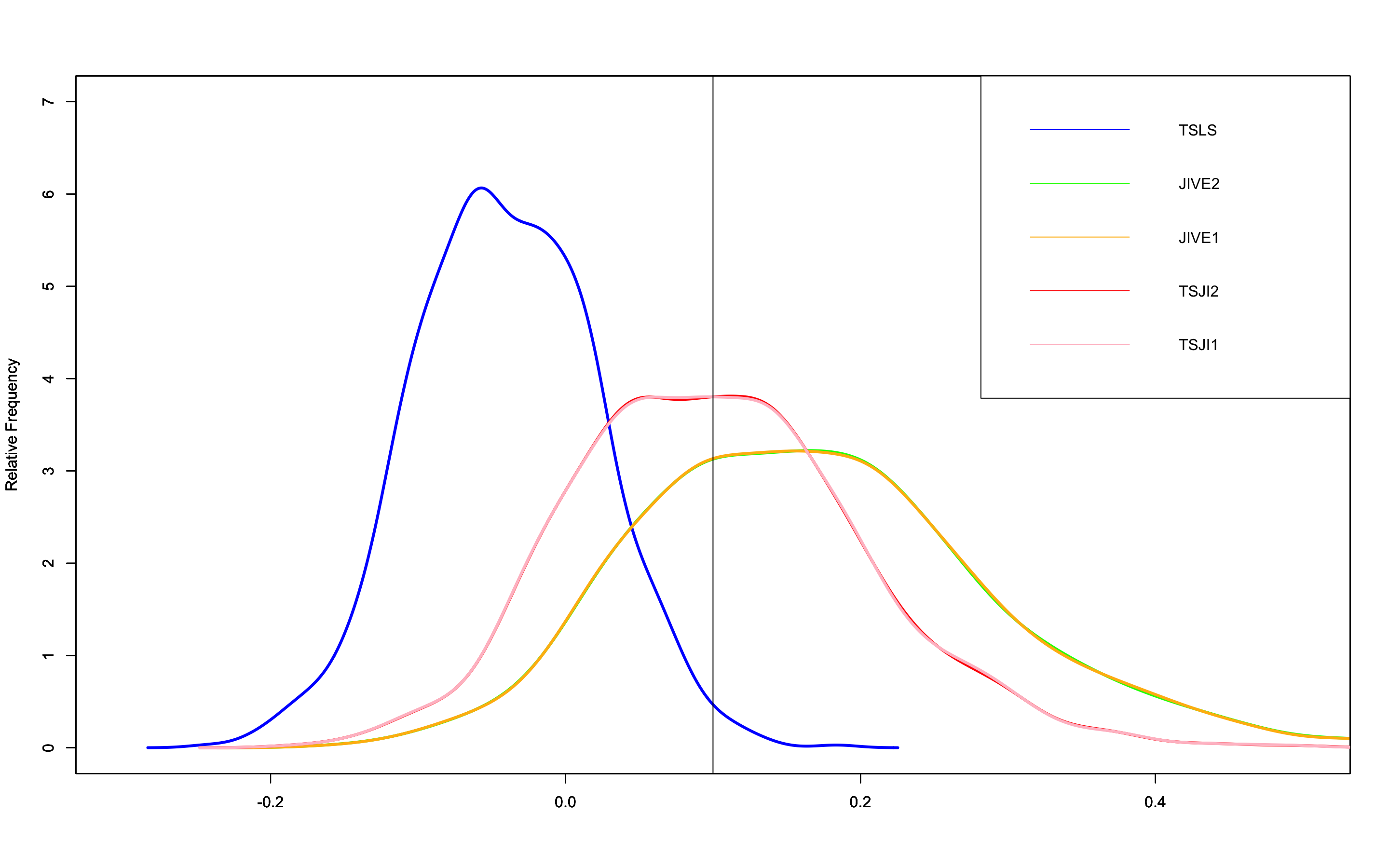
Figure 2: Empirical distributions for TSLS, JIVE and TSJI for the first simulation. The black vertical line is the true $\beta$ value.

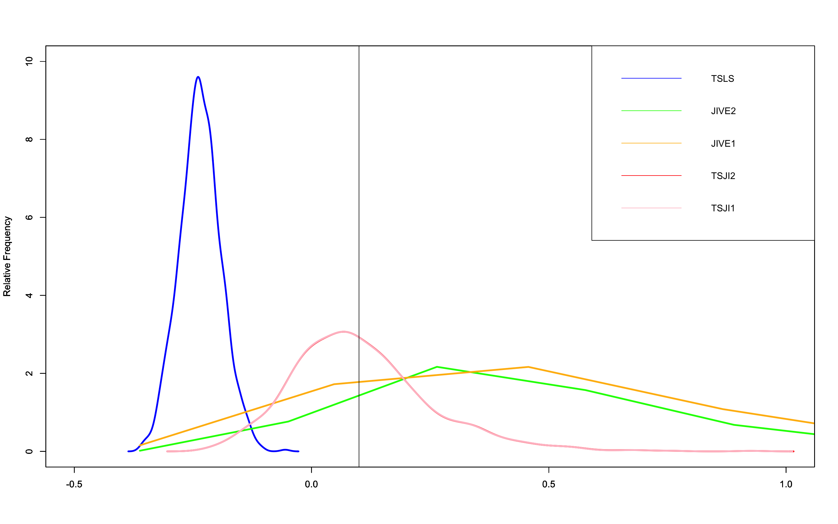
Figure 3: Empirical distributions for TSLS, JIVE and TSJI for the second simulation

I plot the empirical distributions of those 1000 replicates in Figures 2, 3 and 4. The three graphs demonstrate that JIVE’s instability worsens very quickly as the instruments become weaker. The probability density function plot quickly flattens across Figures 2, 3 and 4. The observation aligns with previous findings about JIVE that it lacks moments and hence suffers from large dispersion. TSLS’s bias worsens as the number of instruments becomes larger. The empirical distributions of TSLS depicted in Figures 2, 3 and 4 move further away from $\beta=0.1$. TSJI has the smallest bias as shown in Figures 2, 3 and 4. Most of its mass in terms of empirical distributions are close to the true $\beta$ value. The dispersion of TSJI is also relatively stable as the instruments become weaker. Overall performance of TSJI clearly dominates TSLS and JIVE.

9 Empirical Studies

There are multitudes of social science studies that use a large number of instruments. Some example include the judge leniency IV design where researchers use the identity of judge as instruments. In other words, the number of instruments is equal to the number of judges in the sample. The method has been applied to other settings (See Table 1 in Frandsen et al. (2023) for the immense popularity of judge leniency design). In this section, I apply approximately unbiased TSJI to two classical empirical studies. I compute the standard error by assuming homoskedasticity and treating TSJI as just-identified IV estimator using $\mathring{X}$ as instrument.

9.1 Quarter of birth

The quarter of birth example has been repeatedly cited by many-instrument literature. Here I apply TSJI the famous example in Angrist and Krueger (1991).

Many states in the US has a compulsory school attendance policy. Students are mandated to stay in school until their 16th, 17th or 18th birthday depending on wich state they are from. As such, students’ quarter of birth may induce different quitting-school behavior. This natural experiment makes quarter of birth a valid IV to estimate the marginal earning brought by additional school year for those who are affected by the compulsory attendance policy.

Angrist and Krueger (1991) interacts quarter of birth with other dummy variables to generate a large number of IVs,:

1. Quarter of birth $\times$ Year of birth

2. Quarter of birth $\times$ Year of birth $\times$ State of birth

where case 1 contains 30 instruments, case 2 contains 180 instruments. The results are reported in Table 5.

Case	TSLS	JIVE1	JIVE2	TSJI1	TSJI2
1	8.91	9.59	9.59	9.36	9.36
	(1.61)	(2.22)	(2.22)	(2.01)	(2.01)
2	9.28	12.11	12.11	10.94	10.94
	(0.93)	(1.97)	(1.97)	(1.53)	(1.53)

Table 5: text

9.2 Veteran’s smoking behavior

Bedard and Deschênes (2006) use year of birth and its interaction with gender as instruments to estimate by how much enlisting for WWII and Korean War increase the veterans’ probability in smoking during later part of their life. The result can be interpreted as LATE.

1. Birth year $\times$ gender

2. Birth year

where case 1 uses all data and case 2 uses only data for male veterans. The results are summarized in Table 6.

Case	Dataset	TSLS	JIVE2	JIVE1	TSJI2	TSJI1
1	CPS60	27.6	28.5	28.5	27.8	27.8
		(3.5)	(3.6)	(3.6)	(3.5)	(3.5)
1	CPS90	34.6	35.0	35.0	34.7	34.7
		(2.4)	(2.4)	(2.4)	(2.4)	(2.4)
2	CPS60	23.7	-136.1	-136.1	33.4	33.4
		(13.9)	(224.4)	(224.3)	(22.8)	(22.8)
2	CPS90	30.1	31.1	31.1	30.5	30.5
		(3.2)	(3.3)	(3.3)	(3.2)	(3.2)

Table 6: text

The results of TSLS, JIVE and TSJI are close except for the third row. It is clear that JIVE’s result, which is negative and counterintuitively large in magnitude (larger than 1), is driven by its instability. TSLS and TSJI, though have much closer result in terms of magnitude, point at two different conclusions. TSLS has a test statistics 1.71 whereas TSJI has a test statistics 1.46. Economists who use TSLS are more likely to lower the confidence level of t test to 90% and take the result as a robustness check instead of present it as a main result as did by Bedard and Deschênes (2006). TSJI, on the other hand, suggests a gender difference and time lag for the smoking habit to kick in. Comparing the first row and third row of Table 6, one sees that including women makes the result statistically significant. Comparing third row and fourth, one sees that even though in the sixties, there wasn’t clear difference between veterans and non-veterans in terms of smoking habit; the effect is very prominent in the nineties. Economists who use TSJI are more likely to look at what transpired between the sixties and nineties that impacted veterans and non-veterans differently.

10 Conclusion

Appendix A Approximate bias expansion

Recall that

$$R_{N}=\underbrace{J\epsilon}_{R1}-\underbrace{\frac{Q_{0}}{N}\pi^{\prime}Z^{\prime}\eta J\epsilon}_{R2}+\underbrace{\frac{Q_{0}}{N}\eta^{\prime}C^{\prime}\epsilon}_{R3}-\underbrace{\frac{Q_{0}}{N}\eta^{\prime}C^{\prime}P_{Z\pi}\epsilon}_{R4}+o_{P}(\frac{1}{N})$$

In this section, I will prove corollary 1 and in the process, the derivation of $R1$, $R2$, $R3$ and $R4$. Consider an IV estimator that takes form of $(X^{\prime}C^{\prime}X)^{-1}(X^{\prime}C^{\prime}y)=\beta+(X^{\prime}C^{\prime}X)^{-1}(X^{\prime}C^{\prime}\epsilon)$ where $CZ=Z$ and hence, $CX=Z\pi+\eta$.

$$(X^{\prime}CX)^{-1}(X^{\prime}C\epsilon)= (X^{\prime}CX)^{-1}(X^{\prime}C\epsilon)$$

$$= ((\pi^{\prime}Z^{\prime}+\eta^{\prime}C^{\prime})X)^{-1}(X^{\prime}C^{\prime}\epsilon)$$

$$= (\pi^{\prime}Z^{\prime}X+\eta^{\prime}C^{\prime}X)^{-1}(X^{\prime}C^{\prime}\epsilon)$$

$$= (I+Q\eta^{\prime}C^{\prime}X)^{-1}Q(X^{\prime}C^{\prime}\epsilon)\quad\text{where}\quad Q=(\pi^{\prime}Z^{\prime}X)^{-1}$$

$$= (I-\underbrace{Q\eta^{\prime}C^{\prime}X}_{\sim O_{P}(\frac{1}{\sqrt{N}})})\underbrace{Q(X^{\prime}C^{\prime}\epsilon)}_{\sim O_{P}(\frac{1}{\sqrt{N}})}+o_{P}(\frac{1}{N})$$

The last step is a geometric expansion of $(I+Q\eta^{\prime}C^{\prime}X)^{-1}$ where $Q\eta^{\prime}C^{\prime}X=O_{P}(\frac{1}{\sqrt{N}})$ since $Q=(\pi^{\prime}Z^{\prime}X)^{-1}=O_{P}(\frac{1}{N})$ and $\eta^{\prime}C^{\prime}X=O_{P}(\sqrt{N})$. The first term’s stochastic order is obvious, I evaluate the stochastic order of $\lambda$-class estimator’s $\eta^{\prime}C^{\prime}X$ as an example to show that $\eta^{\prime}C^{\prime}X=O_{P}(\sqrt{N})$. The proof for $\omega$-class is similar but easier given that $\omega\sim O(\frac{1}{N})$ according to corollary 2. The proof for k-class estimator is trivial.

$$\eta^{\prime}C^{\prime}X= \eta^{\prime}(P_{Z}-\lambda D)(I-\lambda D)^{-1}X$$

$$= \eta^{\prime}Z(Z^{\prime}Z)^{-1}Z^{\prime}(I-\lambda D)^{-1}X-\lambda\sum_{i=1}^{N}\eta_{i}^{\prime}Z_{i}(Z^{\prime}Z)^{-1}Z_{i}^{\prime}\frac{X_{i}}{1-\lambda D_{i}}$$

$$= \eta^{\prime}Z(Z^{\prime}Z)^{-1}\sum_{i=1}^{N}\frac{Z_{i}^{\prime}X_{i}}{1-\lambda D_{i}}-\lambda\sum_{i=1}^{N}\eta_{i}^{\prime}D_{i}\frac{X_{i}}{1-\lambda D_{i}}$$

Lemma A.1.

$\eta^{\prime}Z(Z^{\prime}Z)^{-1}\sum_{i=1}^{N}\frac{Z_{i}^{\prime}X_{i}}{1-\lambda D_{i}}=O_{P}(\frac{1}{\sqrt{N}})$.

Proof.

$$\eta^{\prime}Z(Z^{\prime}Z)^{-1}\sum_{i=1}^{N}\frac{Z_{i}^{\prime}X_{i}}{1-\lambda D_{i}}=O_{P}(\sqrt{N})O_{P}(\frac{1}{N})O_{P}(N)=O_{P}(\sqrt{N})$$

because CLT applies to $\frac{1}{\sqrt{N}}\eta^{\prime}Z$ and law of large of number applies to the summation term when divided by $N$. ∎

Assumption 12.

$E[\lVert\eta_{i}^{\prime}X_{i}\rVert^{2+\delta_{1}}]$ is finite, for some $\delta_{1}>0$.

Lemma A.2.

Under assumption 12, $\sum_{i=1}^{N}\eta_{i}^{\prime}D_{i}\frac{X_{i}}{1-\lambda D_{i}}=o_{P}(\sqrt{N})$.

Proof.

$$\lVert\sum_{i=1}^{N}\eta_{i}^{\prime}D_{i}\frac{X_{i}}{1-\lambda D_{i}}\rVert\leq \sum_{i=1}^{N}\lVert\eta_{i}^{\prime}D_{i}\frac{X_{i}}{1-\lambda D_{i}}\rVert$$

$$\leq \frac{1}{1-\lambda}\max_{i}\lVert\eta_{i}^{\prime}X_{i}\rVert\sum_{i=1}^{N}D_{i}$$

$$= \frac{K}{1-\lambda}\max_{i}\lVert\eta_{i}^{\prime}X_{i}\rVert$$

I now show that $\forall\delta>0,P(\frac{K}{(1-\lambda)\sqrt{N}}\max_{i}\lVert\eta_{i}^{\prime}X_{i}\rVert<\delta)\to 1$.

$$P(\frac{K}{1-\lambda}\max_{i}\lVert\eta_{i}^{\prime}X_{i}\rVert<\delta)= P(\max_{i}\lVert\eta_{i}^{\prime}X_{i}\rVert<\frac{(1-\lambda)\delta\sqrt{N}}{K})$$

$$= P(\lVert\eta_{i}^{\prime}X_{i}\rVert<\frac{(1-\lambda)\delta\sqrt{N}}{K}\quad\text{for}\quad i=1,2,\dots,N)$$

$$= P(\lVert\eta_{i}^{\prime}X_{i}\rVert<\frac{(1-\lambda)\delta\sqrt{N}}{K})^{N}$$

$$= P(\lVert\eta_{i}^{\prime}X_{i}\rVert^{2+\delta_{1}}<(\frac{(1-\lambda)\delta\sqrt{N}}{K})^{2+\delta_{1}})^{N}\quad\text{for $\delta_{1}>0$}$$

$$= (1-P(\lVert\eta_{i}^{\prime}X_{i}\rVert^{2+\delta_{1}}\geq(\frac{(1-\lambda)\delta\sqrt{N}}{K})^{2+\delta_{1}}))^{N}$$

$$\geq (1-\frac{E[\lVert\eta_{i}^{\prime}X_{i}\rVert^{2+\delta_{1}}]}{(\frac{(1-\lambda)\delta\sqrt{N}}{K})^{2+\delta_{1}}}))^{N}$$

$$= (1-\frac{1}{N}\frac{E[\lVert\eta_{i}^{\prime}X_{i}\rVert^{2+\delta_{1}}]}{(\frac{(1-\lambda)\delta}{K})^{2+\delta_{1}}N^{\delta_{1}/2}}))^{N}$$

$$\geq 1-\frac{E[\lVert\eta_{i}^{\prime}X_{i}\rVert^{2+\delta_{1}}]}{(\frac{(1-\lambda)\delta}{K})^{2+\delta_{1}}N^{\delta_{1}/2}}\to 1$$

∎

The last inequality holds when $N\geq 1$ and $\frac{E[\lVert X_{i}^{\prime}\epsilon_{i}\rVert^{2+\delta_{1}}]}{(\frac{(1-\lambda)\delta}{K})^{2+\delta_{1}}N^{\delta_{1}/2}}<N$, both of which are true for large $N$. With lemma A.1 and A.2, $\eta^{\prime}C^{\prime}X=O_{P}(\sqrt{N})$. As a result, $Q\eta^{\prime}C^{\prime}X=O_{P}(\frac{1}{\sqrt{N}})$. Similarly, $QX^{\prime}C^{\prime}\epsilon=O_{P}(\frac{1}{\sqrt{N}})$ under assumption 5. The proofs is omitted as the logic is the same as for the proofs for lemma A.1 and A.2.

I sub $X=Z\pi+\eta$ into the $(I-{Q\eta^{\prime}C^{\prime}X})Q(X^{\prime}C^{\prime}\epsilon)+o_{P}(\frac{1}{N})$.

$$(X^{\prime}CX)^{-1}(X^{\prime}C\epsilon)= (I-{Q\eta^{\prime}C^{\prime}(Z\pi+\eta)}Q((Z\pi+\eta)^{\prime}C^{\prime}\epsilon)+o_{P}(\frac{1}{N})$$

$$= (I-Q\eta^{\prime}C^{\prime}Z\pi-Q^{\prime}\eta^{\prime}C^{\prime}\eta)Q(\pi^{\prime}Z^{\prime}\epsilon+\eta^{\prime}C^{\prime}\epsilon)+o_{P}(\frac{1}{N})$$

$$= Q\pi^{\prime}Z^{\prime}\epsilon+Q\eta^{\prime}C^{\prime}\epsilon-Q\eta^{\prime}C^{\prime}Z\pi Q\pi^{\prime}Z^{\prime}\epsilon+o_{P}(\frac{1}{N})$$

The last equality holds because after cross-multiplying, we have six terms to evaluate:

term	stochastic order	keep or not
$Q\pi^{\prime}Z^{\prime}\epsilon$	$O_{P}(\frac{1}{\sqrt{N}})$	Yes
$Q\eta^{\prime}C^{\prime}\epsilon$	$O_{P}(\frac{1}{N})$	Yes
$-Q\eta^{\prime}C^{\prime}Z\pi Q\pi^{\prime}Z^{\prime}\epsilon$	$O_{P}(\frac{1}{N})$	Yes
$-Q\eta^{\prime}C^{\prime}Z\pi Q\eta^{\prime}C^{\prime}\epsilon$	$O_{P}(\frac{1}{N\sqrt{N}})$	No
$-Q\eta^{\prime}C^{\prime}\eta Q\pi^{\prime}Z^{\prime}\epsilon$	$O_{P}(\frac{1}{N\sqrt{N}})$	No
$-Q\eta^{\prime}C^{\prime}\eta Q\eta^{\prime}C^{\prime}\epsilon$	$O_{P}(\frac{1}{N^{2}})$	No

After dropping the last three terms, we obtain the following expression for the difference between the estimator and $\beta$:

$$(X^{\prime}CX)^{-1}(X^{\prime}C\epsilon)=Q\pi^{\prime}Z^{\prime}\epsilon+Q\eta^{\prime}C^{\prime}\epsilon-Q\eta^{\prime}C^{\prime}Z\pi Q\pi^{\prime}Z^{\prime}\epsilon+o_{P}(\frac{1}{N})$$ (21)

We evaluate the three terms in Eq.(21) separately.

A.1 $Q\pi^{\prime}Z^{\prime}\epsilon$

$$Q\pi^{\prime}Z^{\prime}\epsilon= (\pi^{\prime}Z^{\prime}X)^{-1}\pi^{\prime}Z^{\prime}\epsilon$$

$$= (\pi^{\prime}Z^{\prime}Z\pi+\pi^{\prime}Z^{\prime}\eta)^{-1}\pi^{\prime}Z^{\prime}\epsilon$$

$$= \underbrace{(\pi^{\prime}Z^{\prime}Z\pi)^{-1}\pi^{\prime}Z^{\prime}\epsilon}_{E[(\pi^{\prime}Z^{\prime}Z\pi)^{-1}\pi^{\prime}Z^{\prime}\epsilon]=0}-(\pi^{\prime}Z^{\prime}Z\pi)^{-1}\pi^{\prime}Z^{\prime}\eta(\pi^{\prime}Z^{\prime}Z\pi+\pi^{\prime}Z^{\prime}\eta)^{-1}\pi^{\prime}Z^{\prime}\epsilon$$

The part of the expression with a zero expectation is exactly $R1$.

$$(\pi^{\prime}Z^{\prime}Z\pi)^{-1}\pi^{\prime}Z^{\prime}\eta(\pi^{\prime}Z^{\prime}Z\pi+\pi^{\prime}Z^{\prime}\eta)^{-1}\pi^{\prime}Z^{\prime}\epsilon$$

$$= (\pi^{\prime}Z^{\prime}Z\pi)^{-1}\pi^{\prime}Z^{\prime}\eta(\pi^{\prime}Z^{\prime}Z\pi)^{-1}\pi^{\prime}Z^{\prime}\epsilon-\underbrace{(\pi^{\prime}Z^{\prime}Z\pi)^{-1}\pi^{\prime}Z^{\prime}\eta(\pi^{\prime}Z^{\prime}Z\pi)^{-1}\pi^{\prime}Z^{\prime}\eta(\pi^{\prime}Z^{\prime}Z\pi+\pi^{\prime}Z^{\prime}\eta)^{-1}\pi^{\prime}Z^{\prime}\epsilon}_{\sim O_{P}(\frac{1}{N\sqrt{N}})}$$

$$= \underbrace{\frac{Q_{0}}{N}\pi^{\prime}Z^{\prime}\eta(\pi^{\prime}Z^{\prime}Z\pi)^{-1}\pi^{\prime}Z^{\prime}\epsilon}_{R2}+o_{P}(\frac{1}{N})$$

The last equality holds because $N(\pi^{\prime}Z^{\prime}Z\pi)^{-1}\overset{p}{\to}Q_{0}$, therefore, $(\pi^{\prime}Z^{\prime}Z\pi)^{-1}-\frac{Q_{0}}{N}=o_{P}(\frac{1}{N})$. $\pi^{\prime}Z^{\prime}\eta(\pi^{\prime}Z^{\prime}Z\pi)^{-1}\pi^{\prime}Z^{\prime}\epsilon=O_{P}(1)$. So,

$$\frac{Q_{0}}{N}\pi^{\prime}Z^{\prime}\eta(\pi^{\prime}Z^{\prime}Z\pi)^{-1}\pi^{\prime}Z^{\prime}\epsilon-(\pi^{\prime}Z^{\prime}Z\pi)^{-1}\pi^{\prime}Z^{\prime}\eta(\pi^{\prime}Z^{\prime}Z\pi)^{-1}\pi^{\prime}Z^{\prime}\epsilon=o_{P}(\frac{1}{N})O_{P}(1)=o_{P}(\frac{1}{N})$$

$$E[\frac{Q_{0}}{N}\pi^{\prime}Z^{\prime}\eta(\pi^{\prime}Z^{\prime}Z\pi)^{-1}\pi^{\prime}Z^{\prime}\epsilon]= \frac{Q_{0}}{N}E[\pi^{\prime}Z^{\prime}E[\eta(\pi^{\prime}Z^{\prime}Z\pi)^{-1}\pi^{\prime}Z^{\prime}\epsilon|Z]]$$

$$= \frac{Q_{0}}{N}E[\pi^{\prime}Z^{\prime}((\pi^{\prime}Z^{\prime}Z\pi)^{-1}\pi^{\prime}Z^{\prime})^{\prime}]\sigma_{\eta\epsilon}$$

$$= \frac{Q_{0}}{N}I_{L}\sigma_{\eta\epsilon}=\frac{Q_{0}}{N}\sigma_{\eta\epsilon}$$

A.2 $Q\eta^{\prime}C^{\prime}\epsilon$

$$Q\eta^{\prime}C^{\prime}\epsilon=\underbrace{\frac{Q_{0}}{N}\eta^{\prime}C^{\prime}\epsilon}_{R3}+o_{P}(\frac{1}{N})$$

$$E[\frac{Q_{0}}{N}\eta^{\prime}C^{\prime}\epsilon]=\frac{Q_{0}}{N}tr(C^{\prime})\sigma_{\eta\epsilon}$$

A.3 $Q\eta^{\prime}C^{\prime}Z\pi Q\pi^{\prime}Z^{\prime}\epsilon$

$$Q\eta^{\prime}C^{\prime}Z\pi Q\pi^{\prime}Z^{\prime}\epsilon= Q\eta^{\prime}C^{\prime}Z\pi(\pi^{\prime}Z^{\prime}X)^{-1}\pi^{\prime}Z^{\prime}\epsilon$$

$$= Q\eta^{\prime}C^{\prime}Z\pi(\pi^{\prime}Z^{\prime}Z\pi+\pi^{\prime}Z^{\prime}\eta)^{-1}\pi^{\prime}Z^{\prime}\epsilon$$

$$= Q\eta^{\prime}C^{\prime}Z\pi(\pi^{\prime}Z^{\prime}Z\pi)^{-1}\pi^{\prime}Z^{\prime}\epsilon-\underbrace{Q\eta^{\prime}C^{\prime}Z\pi(\pi^{\prime}Z^{\prime}Z\pi)^{-1}\pi^{\prime}Z^{\prime}\eta(\pi^{\prime}Z^{\prime}Z\pi+\pi^{\prime}Z^{\prime}\eta)^{-1}\pi^{\prime}Z^{\prime}\epsilon}_{\sim O(\frac{1}{N\sqrt{N}})}$$

$$= \underbrace{\frac{Q_{0}}{N}\eta^{\prime}C^{\prime}Z\pi(\pi^{\prime}Z^{\prime}Z\pi)^{-1}\pi^{\prime}Z^{\prime}\epsilon}_{R4}+o_{P}(\frac{1}{N})$$

$$E[\frac{Q_{0}}{N}\eta^{\prime}C^{\prime}Z\pi(\pi^{\prime}Z^{\prime}Z\pi)^{-1}\pi^{\prime}Z^{\prime}\epsilon]= \frac{Q_{0}}{N}tr(C^{\prime}Z\pi(\pi^{\prime}Z^{\prime}Z\pi)^{-1}\pi^{\prime}Z^{\prime})\sigma_{\eta\epsilon}$$

$$= \frac{Q_{0}}{N}tr(Z^{\prime}C^{\prime}Z\pi(\pi^{\prime}Z^{\prime}Z\pi)^{-1}\pi^{\prime})\sigma_{\eta\epsilon}$$

$$= \frac{Q_{0}}{N}tr(Z^{\prime}Z\pi(\pi^{\prime}Z^{\prime}Z\pi)^{-1}\pi^{\prime})\sigma_{\eta\epsilon}$$

$$= \frac{Q_{0}}{N}tr(Z\pi(\pi^{\prime}Z^{\prime}Z\pi)^{-1}\pi^{\prime}Z^{\prime})\sigma_{\eta\epsilon}$$

$$= \frac{Q_{0}}{N}tr(P_{Z\pi})\sigma_{\eta\epsilon}$$

Combining the results from sections A.1, A.2 and A.3, we get corollary 1.

Appendix B Bridging TSLS and JIVEs

Angrist et al. (1995) show that the approximate biases of TSLS and JIVE are as following respectively:

$$\frac{K-L-1}{N}Q_{0}\sigma_{\epsilon\eta}$$

$$-\frac{L+1}{N}Q_{0}\sigma_{\epsilon\eta}$$

The contrast between the two approximate bias terms are very interesting. Fix the number of endogenous variables, the bias of TSLS increases with the number of instruments ($K-L=$ degree of overidentification $=$ number of instruments$-1$); the bias of JIVE increases with the number of control variables (L = number of endogenous variables $+$ number of control variables). As a result, these two estimators have large bias when the second-stage equation is large and the first-stage equation is even much larger. But the biases have opposite signs. The different signs of the bias expressions suggest that combining these two estimators can potentially give us an approximately unbiased estimator, no matter how big Eqs. (3) and (4) are.

Bridging the optimization problems of TSLS and the two forms of JIVE, I derive two new estimators (TSJI2 and TSJI1) from the connected optimization problems. The optimization problems of TSLS and JIVE2 are Eqs. (22) and (23), respectively:

$$\min_{\beta}(y-X\beta)^{\prime}P(y-X\beta) =\min_{\beta}\sum_{i,j}(y_{i}-X_{i}\beta)^{\prime}P_{ij}(y_{j}-X_{j}\beta)$$ (22)

$$=\min_{\beta}\sum_{i\neq j}(y_{i}-X_{i}\beta)^{\prime}P_{ij}(y_{j}-X_{j}\beta)+{\color[rgb]{1,0,0}\sum_{i=1}^{n}(y_{i}-X_{i}\beta)P_{ii}(y_{i}-X_{i}\beta)}$$

where $\sum_{i,j}=\sum_{i=1}^{n}\sum_{j=1}^{n}$ and $P_{ij}$ denotes (i,j) entry of $P$.

$$\min_{\beta}\sum_{i\neq j}(y_{i}-X_{i}\beta)P_{ij}(y_{j}-X_{j}\beta)$$ (23)

where $\sum_{i\neq j}=\sum_{i=1}^{n}\sum_{j\neq i}$. The only difference from the optimization problem of TSLS is the red text in minimization problem (22). A user-defined parameter $1-\lambda\in[0,1]$ is placed in front this term and a new optimization problem that bridges TSLS and JIVE2 is obtained as Eq. (24). When $\lambda=0$, the solution of minimization problem (24) is TSLS; when $\lambda=1$, the solution of it is JIVE2.

$$\min_{\beta}\sum_{j\neq i}(y_{i}-X_{i}\beta)P_{ij}(y_{j}-X_{j}\beta)+{\color[rgb]{1,0,0}(1-\lambda)}\sum_{i=1}^{n}(y_{i}-X_{i}\beta)P_{ii}(y_{i}-X_{i}\beta)$$ (24)

Solving minimization problem (24), I get a new estimator (TSJI2) which can be written in matrix operation:

$$\mathring{\beta}_{TSJI2} =\bigg{(}\sum_{i\neq j}X_{i}^{\prime}P_{ij}X_{j}+(1-\lambda)\sum_{i}X_{i}^{\prime}P_{ii}X_{i}\bigg{)}^{-1}\bigg{(}\sum_{i\neq j}X_{i}^{\prime}P_{ij}y_{j}+(1-\lambda)\sum_{i}X_{i}^{\prime}P_{ii}y_{i}\bigg{)}$$ (25)

$$=\big{(}X^{\prime}PX-\lambda X^{\prime}DX\big{)}^{-1}\big{(}X^{\prime}Py-\lambda X^{\prime}Dy\big{)}$$

$$=\big{(}X^{\prime}(P-\lambda D)X\big{)}^{-1}\big{(}X^{\prime}(P-\lambda D)y\big{)}$$

where D is the diagonal matrix of $P$.

The connection between JIVE1 and TSLS is little more complicated. The optimization problem of JIVE1 is:

$$\min_{\beta}\sum_{i\neq j}(y_{i}-X_{i}\beta)\frac{P_{ij}}{1-P_{jj}}(y_{j}-X_{j}\beta)$$ (26)

I bridge optimization problems (26) and (22) by placing a user-fined parameter $\lambda\in[0,1]$ at three separate locations. The new estimator (TSJI1) solves the following optimization problem:

$$\min_{\beta}\sum_{j\neq i}(y_{i}-X_{i}\beta)\frac{P_{ij}}{1-{\color[rgb]{1,0,0}\lambda}P_{jj}}(y_{j}-X_{j}\beta)+\sum_{i=1}^{N}(y_{i}-X_{i}\beta)\frac{(1-{\color[rgb]{1,0,0}\lambda})P_{ii}}{1-{\color[rgb]{1,0,0}\lambda}P_{ii}}(y_{i}-X_{i}\beta)$$ (27)

When $\lambda=1$, the optimization problem is the same as minimization problem (26), whereas when $\lambda=0$, the optimization problem is the same as formula (22). Solving minimization problem (27), I obtain a new estimator (TSJI1):

$$\mathring{\beta}_{TSJI1}=(X^{\prime}[(I-\lambda D)^{-1}(P-\lambda D)]^{\prime}X)^{-1}(X^{\prime}[(I-\lambda D)^{-1}(P-\lambda D)]^{\prime}y)$$ (28)

Appendix C Proof of expression (6)

C.1 Results from Corollary 1

Corollary 1 states that the approximate bias of $\lambda$-class estimator is proportional to $tr(C^{\prime})-tr(P_{Z\pi})-1$.

$$tr\{C^{\prime}\} =tr\{C\}=tr\{(I-\lambda D)^{-1}(P-\lambda D)\}=(1-\lambda)\sum_{i=1}^{N}\frac{D_{i}}{1-\lambda D_{i}}$$

$$tr(P_{Z\pi}) =tr\{Z\pi(\pi^{\prime}Z^{\prime}Z\pi)^{-1}\pi^{\prime}Z^{\prime}\}=tr\{\pi^{\prime}Z^{\prime}Z\pi(\pi^{\prime}Z^{\prime}Z\pi)^{-1}\}=tr\{I_{L}\}=L$$

Therefore, the approximate bias of TSJI1 is proportional to $E[(1-\lambda)\sum_{i=1}^{N}\frac{D_{i}}{1-\lambda D_{i}}]-L-1$.

C.2 Computation of $\lambda$

We can obtain a sample analogue of $E[(1-\lambda)\sum_{i=1}^{N}\frac{D_{i}}{1-\lambda D_{i}}]-L-1$ by simply dropping the expectation. We then solve

$$(1-\lambda)\sum_{i=1}^{N}\frac{D_{i}}{1-\lambda D_{i}}-L-1=0$$ (7)

to obtain $\lambda$ that gives an approximately unbiased TSJI1.

Equation (7) is of order N+1 with respect to $\lambda$. Obtaining a closed-form solution is, therefore, infeasible. On the other hand, numerical solution of Equation (7) is readily available since the left hand side of the equation is a strictly decreasing function of $\lambda$ when $\lambda\in(0,1)$. When $\lambda=0$, the LHS expression takes on a strictly positive value $K-L-1$; when $\lambda=0$, the LHS expression takes on a strictly negative value $-L-1$. We can do a bisection search to quickly pin down the unique $\lambda$ value that gives an approximately unbiased TSJI1.

Figure 4: Empirical distributions for TSLS, JIVE and TSJI for the third simulation

References

- Ackerberg and Devereux (2009) Daniel A Ackerberg and Paul J Devereux. Improved jive estimators for overidentified linear models with and without heteroskedasticity. The Review of Economics and Statistics, 91(2):351–362, 2009.
- Amuedo-Dorantes and Pozo (2014) Catalina Amuedo-Dorantes and Susan Pozo. When do remittances facilitate asset accumulation? the importance of remittance income uncertainty. 2014.
- Amuedo-Dorantes et al. (2010) Catalina Amuedo-Dorantes, Annie Georges, and Susan Pozo. Migration, remittances, and children’s schooling in haiti. The Annals of the American Academy of Political and Social Science, 630(1):224–244, 2010.
- Andrews and Armstrong (2017) Isaiah Andrews and Timothy B Armstrong. Unbiased instrumental variables estimation under known first-stage sign. Quantitative Economics, 8(2):479–503, 2017.